





1. Introduction
Dusty plasma is a system composed of electrons, ions, neutral particles and charged dust grains (Du et al. Reference Du2012; Thomas et al. Reference Thomas, Konopka, Merlino and Rosenberg2016; Davletov, Kurbanov & Mukhametkarimov Reference Davletov, Kurbanov and Mukhametkarimov2020; Beckers et al. Reference Beckers2023; Lu et al. Reference Lu, Huang, Liang and Feng2025; Williams et al. Reference Williams, Royer, Thakur, Thomas and Williams2025). Current research on dusty plasmas primarily focuses on several areas, including dust-related phenomena in natural environments such as planetary rings (Havnes et al. Reference Havnes, Aslaksen, Hartquist, Li, Melandsø, Morfill and Nitter1995; Gong et al. Reference Gong, Ivlev, Akimkin and Caselli2021; Jiang & Du Reference Jiang and Du2022) and the mesosphere (Sternovsky et al. Reference Sternovsky, Holzworth, Horányi and Robertson2004; Popel & Dubinsky Reference Popel and Dubinsky2013), various plasma–particle interactions (Shukla & Eliasson Reference Shukla and Eliasson2009; Kompaneets, Morfill & Ivlev Reference Kompaneets, Morfill and Ivlev2016), particle growth and fusion in industrial applications (Santos et al. Reference Santos, Reeves, Michael, Tan, Wise and Bilek2019; Nespoli et al. Reference Nespoli2022), many-body physics (Thoma et al. Reference Thoma, Thomas, Knapek, Melzer and Konopka2023), and fundamental problems in condensed matter (Morfill & Ivlev Reference Morfill and Ivlev2009; Chaudhuri et al. Reference Chaudhuri, Ivlev, Khrapak, Thomas and Morfill2011). Over the past decades, one of the most significant breakthroughs in dusty plasma physics has been the experimental discovery of dust lattice structures (Hayashi & Tachibana Reference Hayashi and Tachibana1994; Chu & Lin Reference Chu and Lin1994; Melzer, Trottenberg & Piel Reference Melzer, Trottenberg and Piel1994; Thomas et al. Reference Thomas, Morfill, Demmel, Goree, Feuerbacher and Möhlmann1994). Subsequently, dust lattice waves were observed within these ordered systems (Melandsø Reference Melandsø1996; Homann et al. Reference Homann, Melzer, Peters and Piel1997). This discovery not only confirmed that dust particles can spontaneously form crystal-like ordered structures under strongly coupled conditions, but also provided a solid foundation for the study of wave propagation and collective behaviours in dusty plasmas.
In 1996, Melandsø (Reference Melandsø1996) first investigated wave propagation in one-dimensional dusty plasma lattices, and this theoretical work laid the foundation for subsequent experimental studies. Then, Homann et al. (Reference Homann, Melzer, Peters and Piel1997) experimentally observed dust lattice waves and subsequently extended the study to two-dimensional dusty plasma systems (Homann et al. Reference Homann, Melzer, Peters, Madani and Piel1998). Huang et al. (Reference Huang, Ivlev, Nosenko, Lin and Du2019) first investigated the square lattice structures in two-dimensional binary complex plasmas, and then Singh et al. (Reference Singh, Bandyopadhyay, Kumar and Sen2022) achieved the observation of a square lattice formation in a monodisperse complex plasma system. The propagation characteristics of linear waves have been extensively investigated through experiments, theoretical analyses and numerical simulations (Vladimirov, Shevchenko & Cramer Reference Vladimirov, Shevchenko and Cramer1997; Otani, Bhattacharjee & Wang Reference Otani, Bhattacharjee and Wang1999; Ivlev & Morfill Reference Ivlev and Morfill2000; Misawa et al. Reference Misawa, Ohno, Asano, Sawai, Takamura and Kaw2001; Nunomura et al. Reference Nunomura, Goree, Hu, Wang, Bhattacharjee and Avinash2002; Liu, Avinash & Goree Reference Liu, Avinash and Goree2003; Farokhi, Kourakis & Shukla Reference Farokhi, Kourakis and Shukla2006; Wang et al. Reference Wang, Duan, Lin and Wan2006; Bandyopadhyay et al. Reference Bandyopadhyay, Prasad, Sen and Kaw2008; Farokhi & Hameditabar Reference Farokhi and Hameditabar2012; Lipaev et al. Reference Lipaev, Naumkin, Khrapak, Usachev, Petrov, Thoma, Kretschmer, Du, Kononenko and Zobnin2025). In recent years, research has gradually shifted towards nonlinear phenomena in dust lattice waves, including solitary waves (Avinash et al. Reference Avinash, Zhu, Nosenko and Goree2003; Sheridan, Nosenko & Goree Reference Sheridan, Nosenko and Goree2008; Tian-Jun Reference Tian-Jun2009; Ghosh & Gupta Reference Ghosh and Gupta2010; Hong et al. Reference Hong, Sun, Schwabe, Du and Duan2021; Wei et al. Reference Wei, Peng, Yang, Du, Yang and Duan2023a ; Huang et al. Reference Huang, Ivlev, Nosenko, Yang and Du2023), shock waves (Ghosh Reference Ghosh2008a , Reference Ghoshb , Reference Ghosh2009; Kananovich & Goree Reference Kananovich and Goree2020; Niu, Tian & Chen Reference Niu, Tian and Chen2020; Ding et al. Reference Ding, Lu, Sun, Murillo and Feng2021; Wei et al. Reference Wei, Peng, Yang, Yang and Duan2023b ) and breathers (Kourakis & Shukla Reference Kourakis and Shukla2005; Koukouloyannis & Kourakis Reference Koukouloyannis and Kourakis2009; Koukouloyannis et al. Reference Koukouloyannis, Kevrekidis, Law, Kourakis and Frantzeskakis2010). These nonlinear phenomena have attracted considerable attention due to their significance in energy transport applications and wave dynamics control in controlled environments.
In the field of nonlinear wave research, envelope waves, as a significant nonlinear structures, have garnered considerable attention in dusty plasma lattice systems (Ivlev, Zhdanov & Morfill Reference Ivlev, Zhdanov and Morfill2003; Kourakis & Shukla Reference Kourakis and Shukla2004,Reference Kourakis and Shukla2006; Togueu Motcheyo et al. Reference Togueu Motcheyo, Nkendji Kenkeu, Djako and Tchawoua2018; Nkendji Kenkeu et al. Reference Nkendji Kenkeu, Togueu Motcheyo, Kanaa and Tchawoua2022; Houwe et al. Reference Houwe, Abbagari, Inc, Betchewe, Doka and Crépin2022; Shi et al. Reference Shi, Wei, Yang, Yang and Duan2024; Han et al. Reference Han, Shi, Yang and Duan2025). Togueu Motcheyo et al. (Reference Togueu Motcheyo, Nkendji Kenkeu, Djako and Tchawoua2018) numerically demonstrated that envelope bright solitons can propagate stably within dusty plasma lattices. Subsequently, Houwe et al. (Reference Houwe, Abbagari, Inc, Betchewe, Doka and Crépin2022) further investigated the propagation dynamics of envelope solitons under vertical oscillations of dust grains based on the nonlinear Schrödinger equation (NLSE). They elucidated the formation mechanisms of bright and dark solitons in different frequency regimes and confirmed the validity of their theoretical predictions through numerical simulations. Notably, envelope waves have been extensively studied not only in dusty plasma lattices, but also across various disciplines, including fluid mechanics (Osborne Reference Osborne2002; Slunyaev et al. Reference Slunyaev, Clauss, Klein and Onorato2013; Gandzha & Sedletsky Reference Gandzha and Sedletsky2017; Stepanyants Reference Stepanyants2019; Liao et al. Reference Liao, Dong, Ma and Ma2023) and nonlinear optics (Karjanto Reference Karjanto2022; Wazwaz et al. Reference Wazwaz, Alyousef, Ismaeel and El-Tantawy2023; Omar et al. Reference Omar, Murad, Mahmood, Malik and Radwan2025). These interdisciplinary efforts have provided a solid theoretical foundation for understanding the formation and evolution of envelope waves. However, most existing studies on envelope solitons are restricted to analytical solutions of the NLSE. In this work, we overcome this limitation by employing numerical simulations. We demonstrate the existence of bright solitons that do not conform to the standard analytical envelope bright soliton solutions of the NLSE, and systematically investigate their propagation characteristics and stability. This discovery significantly advances the theoretical framework of nonlinear waves in dusty plasmas and other nonlinear systems.
The rest of this paper is organised as follows. In § 2, establishes the model used for the present study. In § 3, a systematic investigation is conducted on the propagation properties and stability of arbitrarily prescribed envelope waves and general waveforms in a one-dimensional dusty plasma chain. Section 4 presents the conclusion for the present paper.
2. Model
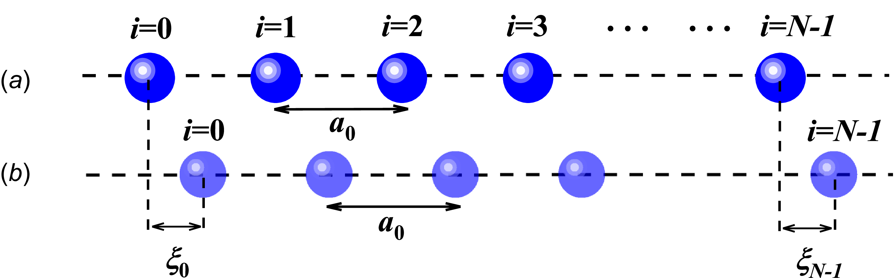
We consider an homogeneous dust particle chain in which all particles are identical within the range $i = 0$
to
$i = 0$
to $i = N-1$
, as illustrated in figure 1. The present study focuses on what kind of the envelope waves exists in the system.
$i = N-1$
, as illustrated in figure 1. The present study focuses on what kind of the envelope waves exists in the system.
The position of the $i{\mathrm{th}}$
dust particle is assumed to be
$i{\mathrm{th}}$
dust particle is assumed to be $x_i = i a_0 + \xi _i$
, where
$x_i = i a_0 + \xi _i$
, where $\xi _i$
represents the displacement from its equilibrium position
$\xi _i$
represents the displacement from its equilibrium position $i a_0$
and
$i a_0$
and $a_0$
is the lattice constant. The equation of motion governing an arbitrary dust particle
$a_0$
is the lattice constant. The equation of motion governing an arbitrary dust particle $i$
is given by
$i$
is given by $ m_{d}\ddot {\bf{\xi }}_i= -{Q_d} \boldsymbol{\nabla }\sum \nolimits _{j\neq i} \phi _{ij}$
, where
$ m_{d}\ddot {\bf{\xi }}_i= -{Q_d} \boldsymbol{\nabla }\sum \nolimits _{j\neq i} \phi _{ij}$
, where $m_{d}$
and
$m_{d}$
and $Q_d$
are the mass and charge of the dust particle,
$Q_d$
are the mass and charge of the dust particle, $\phi _{ij}$
is the Yukawa interaction potential between dust particles of
$\phi _{ij}$
is the Yukawa interaction potential between dust particles of $i$
and
$i$
and $j$
,
$j$
, $\phi _{ij} = ({Q_d / 4\pi \varepsilon _{0} x_{ij})}e^{-{x_{ij} / \lambda _D}}$
, where
$\phi _{ij} = ({Q_d / 4\pi \varepsilon _{0} x_{ij})}e^{-{x_{ij} / \lambda _D}}$
, where $x_{ij}=|x_{i}-x_{j}|$
is the distance between dust particles
$x_{ij}=|x_{i}-x_{j}|$
is the distance between dust particles $i$
and
$i$
and $j$
,
$j$
, $\lambda _D$
is the Debye length, and
$\lambda _D$
is the Debye length, and $\varepsilon _{0}$
is the permittivity of vacuum.
$\varepsilon _{0}$
is the permittivity of vacuum.
By using the small amplitude approximation $a_{0}\gg \xi _{i}-\xi _{i-1}$
, the long-wavelength approximation
$a_{0}\gg \xi _{i}-\xi _{i-1}$
, the long-wavelength approximation $a_0\ll \lambda _w$
, where
$a_0\ll \lambda _w$
, where $\lambda _w$
is the wavelength of the perturbations, as well as the continuum approximation
$\lambda _w$
is the wavelength of the perturbations, as well as the continuum approximation $\xi _i(t)=\xi (x, t)$
, we have (Wei et al. Reference Wei, Peng, Yang, Du, Yang and Duan2023a
)
$\xi _i(t)=\xi (x, t)$
, we have (Wei et al. Reference Wei, Peng, Yang, Du, Yang and Duan2023a
)
 \begin{equation} \frac {\partial ^{2}{\xi }}{\partial {t}^{2}}= B_{1}\left(\frac {\partial ^{2}{\xi }}{\partial {x}^{2}} +\frac {a_{0}^{2}}{12}\frac {\partial ^{4}{\xi }}{\partial {x}^{4}}\right)+ B_{2}\frac {\partial {\xi }}{\partial {x}} \frac {\partial ^{2}{\xi }}{\partial {x}^{2}}, \end{equation}
where $B_{1}={k_{1}a_{0}^{2}}/{m_{d}}$
,
$B_{1}={k_{1}a_{0}^{2}}/{m_{d}}$
, $B_{2}={2k_{2}a_{0}^{3}}/{m_{d}}$
,
$B_{2}={2k_{2}a_{0}^{3}}/{m_{d}}$
, $k_{1} =({Q_{d}^{2}}/{4\pi \varepsilon _{0}a_{0}^{3})}e^{-\kappa }[2+2\kappa +\kappa ^{2}]$
,
$k_{1} =({Q_{d}^{2}}/{4\pi \varepsilon _{0}a_{0}^{3})}e^{-\kappa }[2+2\kappa +\kappa ^{2}]$
, $k_{2} = - ({Q_{d}^{2}}/{8\pi \varepsilon _{0}a_{0}^{4})}e^{-\kappa }[6+6\kappa +3\kappa ^{2}+\kappa ^{3}]$
,
$k_{2} = - ({Q_{d}^{2}}/{8\pi \varepsilon _{0}a_{0}^{4})}e^{-\kappa }[6+6\kappa +3\kappa ^{2}+\kappa ^{3}]$
, $\kappa ={a_0 /\lambda _D}$
.
$\kappa ={a_0 /\lambda _D}$
.
Schematics of a dust particle chain, in which the blue spheres are dust particles labelled from $i=0$
to
$i=0$
to $i=N-1$
. (a) Arrangement of dust particles at their equilibrium positions, with
$i=N-1$
. (a) Arrangement of dust particles at their equilibrium positions, with $a_0$
denoting the lattice constant; (b) Configuration when the dust particles are displaced from their equilibrium position, where
$a_0$
denoting the lattice constant; (b) Configuration when the dust particles are displaced from their equilibrium position, where $\xi _i$
represents the displacement of the
$\xi _i$
represents the displacement of the $i$
th dust particle from its equilibrium position.
$i$
th dust particle from its equilibrium position.

3. Propagation characteristics of waves in an homogeneous dusty plasma
3.1. Influence of the nonlinear parameter $\alpha$
on the propagation characteristics of the envelope wave
$\alpha$
on the propagation characteristics of the envelope wave

In the following, we introduce the stretched coordinates $\eta = \varepsilon (x- V t)$
,
$\eta = \varepsilon (x- V t)$
, $\tau = \varepsilon ^{2}t$
by using the traditional reductive perturbation method (Zhang et al. Reference Zhang, Qi, Duan and Yang2015; Gao et al. Reference Gao, Zhang, Zhang, Li and Duan2017), where
$\tau = \varepsilon ^{2}t$
by using the traditional reductive perturbation method (Zhang et al. Reference Zhang, Qi, Duan and Yang2015; Gao et al. Reference Gao, Zhang, Zhang, Li and Duan2017), where $ \varepsilon$
is a small parameter and
$ \varepsilon$
is a small parameter and $V$
is the velocity of the wave. The quantity of
$V$
is the velocity of the wave. The quantity of $\xi$
is expanded as
$\xi$
is expanded as $ \xi = \sum _{n=1}^\infty \varepsilon ^n \sum _{l=-\infty }^{+\infty }\xi ^{(n,l)}(\eta , \tau )e^{il(kx-\omega t)}$
.
$ \xi = \sum _{n=1}^\infty \varepsilon ^n \sum _{l=-\infty }^{+\infty }\xi ^{(n,l)}(\eta , \tau )e^{il(kx-\omega t)}$
.
Substituting these expansions into (2.1) and separation of terms according to the first three powers of $\varepsilon$
yields dispersion relation of (see Appendix A)
$\varepsilon$
yields dispersion relation of (see Appendix A) $ \omega ^2= B_1k^2[1-({a_0^2 / 12)} k^2]$
, the group velocity of
$ \omega ^2= B_1k^2[1-({a_0^2 / 12)} k^2]$
, the group velocity of $ V= B_1{k / \omega }[1-({a_0^2 / 6}) k^2]$
and NLSE as follows:
$ V= B_1{k / \omega }[1-({a_0^2 / 6}) k^2]$
and NLSE as follows: $ i({\partial \xi ^{(1,1)} / \partial \tau } )+P({\partial ^2 \xi ^{(1,1)} / \partial \eta ^2 } )+Q\xi ^{(1,1)}\mid \xi ^{(1,1)}\mid ^2 =0$
, where
$ i({\partial \xi ^{(1,1)} / \partial \tau } )+P({\partial ^2 \xi ^{(1,1)} / \partial \eta ^2 } )+Q\xi ^{(1,1)}\mid \xi ^{(1,1)}\mid ^2 =0$
, where $P = ({{2{B_1} - 2{V^2} - {B_1}a_0^2{k^2}}})/{{4\omega }}$
,
$P = ({{2{B_1} - 2{V^2} - {B_1}a_0^2{k^2}}})/{{4\omega }}$
, $Q={3 B_2^2 k^6 / (-12\omega ^3+12\omega k^2 B_1-4\omega B_1 a_0^2 k^4)}$
. In the experimental coordinates, we have one envelope wave solution of NLSE as follows:
$Q={3 B_2^2 k^6 / (-12\omega ^3+12\omega k^2 B_1-4\omega B_1 a_0^2 k^4)}$
. In the experimental coordinates, we have one envelope wave solution of NLSE as follows:
 \begin{equation} \xi _i=A \textrm {sech}[w(x-Vt)] \textrm {e}^{\textrm {i}[k_bx-\omega _b t]}, \end{equation}
where $A= \varepsilon \sqrt {{2(Pk^2-\omega ) / Q}}$
is the envelope wave amplitude,
$A= \varepsilon \sqrt {{2(Pk^2-\omega ) / Q}}$
is the envelope wave amplitude, $w= {\varepsilon }\sqrt {{(Pk^2-\omega ) / P}}$
the envelope wave width,
$w= {\varepsilon }\sqrt {{(Pk^2-\omega ) / P}}$
the envelope wave width, $V$
is the envelope wave group velocity and
$V$
is the envelope wave group velocity and $k_{b}={k( {\varepsilon + 1} )}$
the background wave frequency of the envelope wave,
$k_{b}={k( {\varepsilon + 1} )}$
the background wave frequency of the envelope wave, $\omega _{b}={( {k{V}\varepsilon + \omega {\varepsilon ^2} + \omega } )}$
. The envelope wave solution of (3.1) has been verified numerically and experimentally (Zhang et al. Reference Zhang, Qi, Duan and Yang2015; Gao et al. Reference Gao, Zhang, Zhang, Li and Duan2017; Jahan et al. Reference Jahan, Chowdhury, Mannan and Mamun2019; Houwe et al. Reference Houwe, Abbagari, Inc, Betchewe, Doka and Crépin2022).
$\omega _{b}={( {k{V}\varepsilon + \omega {\varepsilon ^2} + \omega } )}$
. The envelope wave solution of (3.1) has been verified numerically and experimentally (Zhang et al. Reference Zhang, Qi, Duan and Yang2015; Gao et al. Reference Gao, Zhang, Zhang, Li and Duan2017; Jahan et al. Reference Jahan, Chowdhury, Mannan and Mamun2019; Houwe et al. Reference Houwe, Abbagari, Inc, Betchewe, Doka and Crépin2022).
To further explore the envelope wave solutions in this system, we assume that there is an arbitrary envelope wave as follows:
 \begin{equation} \xi _i=A \textrm {sech}[\alpha w(x-Vt)] \textrm {e}^{\textrm {i}[k_bx-\omega _b t]}, \end{equation}
where $\alpha$
is an arbitrary constant. It is obvious that (3.2) is not a solution of the NLSE when
$\alpha$
is an arbitrary constant. It is obvious that (3.2) is not a solution of the NLSE when $\alpha \ne 1$
. However, in the present paper, we try to verify that the envelope wave expressed by (3.2) actually exist in the system.
$\alpha \ne 1$
. However, in the present paper, we try to verify that the envelope wave expressed by (3.2) actually exist in the system.
To verify it, we perform a molecular dynamical simulations using the Large-scale Atomic/Molecular Massively Parallel Simulator (Sandia National Laboratories n.d.). We assume that each dust particle is a negative point charge and they are arranged as a chain. We place a chain of $N=25\,000$
identical dust particles from
$N=25\,000$
identical dust particles from $i=0$
to
$i=0$
to $i=24\,999$
, and choose typical plasma and particle parameters according to the literature (Sun et al. Reference Sun2018; Du et al. Reference Du, Nosenko, Thomas, Lin, Morfill and Ivlev2019; Huang et al. Reference Huang, Schwabe, Thomas, Lipaev and Du2021):
$i=24\,999$
, and choose typical plasma and particle parameters according to the literature (Sun et al. Reference Sun2018; Du et al. Reference Du, Nosenko, Thomas, Lin, Morfill and Ivlev2019; Huang et al. Reference Huang, Schwabe, Thomas, Lipaev and Du2021): $a_{0}=0.8$
mm,
$a_{0}=0.8$
mm, $\lambda _{D}=0.4$
mm,
$\lambda _{D}=0.4$
mm, $Q_{d}=2700e$
,
$Q_{d}=2700e$
, $e$
represents the elementary charge,
$e$
represents the elementary charge, $m_{d}=3.6\times 10^{-15}$
kg and the diameter of each dust particle is
$m_{d}=3.6\times 10^{-15}$
kg and the diameter of each dust particle is $d=1.55$ $\mu$
m. The time step of the simulation is
$\mu$
m. The time step of the simulation is $\mathrm{d}t=1.0\times 10^{-4}$
s. For simplicity, we assume that the dust particle temperature is zero. We also assume that an envelope wave which satisfies (3.2) exists in the dusty lattice chain. Based on these assumptions, the initial displacements of all dust particles from their equilibrium positions and their corresponding velocities are determined from (3.2).
$\mathrm{d}t=1.0\times 10^{-4}$
s. For simplicity, we assume that the dust particle temperature is zero. We also assume that an envelope wave which satisfies (3.2) exists in the dusty lattice chain. Based on these assumptions, the initial displacements of all dust particles from their equilibrium positions and their corresponding velocities are determined from (3.2).
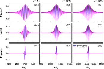
Comparison between MD simulation results and analytical results of envelope waves in a one-dimensional dusty particle chain under different parameters: (a1–a3) $\alpha =0.5$
, (b1–b3)
$\alpha =0.5$
, (b1–b3) $\alpha =1.0$
, (c1–c3)
$\alpha =1.0$
, (c1–c3) $\alpha =5.0$
) and at different times (
$\alpha =5.0$
) and at different times ( $t=150$
s and
$t=150$
s and $t=350$
s), which is given by (3.2). The analytical results are represented by blue solid lines, while the numerical ones are expressed by magenta dots.
$t=350$
s), which is given by (3.2). The analytical results are represented by blue solid lines, while the numerical ones are expressed by magenta dots.

Figure 2 illustrates the temporal evolution of the velocity profile of an envelope wave in a one-dimensional dusty plasma chain under varying nonlinear parameter values ( $\alpha$
= 0.5, 1.0, 5.0), which is given by (3.2). The parameter
$\alpha$
= 0.5, 1.0, 5.0), which is given by (3.2). The parameter $\alpha$
inside the sech function is arbitrarily assigned. As
$\alpha$
inside the sech function is arbitrarily assigned. As $\alpha$
increases, the envelope becomes narrower and more localised. The consistency between analytical (solid lines) and numerical (dots) results confirms that such artificially constructed waveforms can propagate stably within the system.
$\alpha$
increases, the envelope becomes narrower and more localised. The consistency between analytical (solid lines) and numerical (dots) results confirms that such artificially constructed waveforms can propagate stably within the system.
The results presented in figure 2 demonstrate that the constructed envelop wave can propagate stably under various parameters $\alpha$
. It is an envelope solitary wave. However, there is a question whether it is a soliton. To verify it, we proceed to investigate head-on collisions between two envelop waves with different values of
$\alpha$
. It is an envelope solitary wave. However, there is a question whether it is a soliton. To verify it, we proceed to investigate head-on collisions between two envelop waves with different values of $\alpha$
.
$\alpha$
.
There are two solutions of the dispersion relation $\omega ^2= B_1k^2[1-{(a_0^2 / 12)} k^2]$
. We defined
$\omega ^2= B_1k^2[1-{(a_0^2 / 12)} k^2]$
. We defined $\omega _1 =\sqrt {B_1(1-({a_0^2 / 12}) k^2)}k$
,
$\omega _1 =\sqrt {B_1(1-({a_0^2 / 12}) k^2)}k$
, $\omega _2 =-\sqrt {B_1(1-({a_0^2 / 12}) k^2)}k$
. When
$\omega _2 =-\sqrt {B_1(1-({a_0^2 / 12}) k^2)}k$
. When $\omega \gt 0$
, the envelope wave propagates in the positive
$\omega \gt 0$
, the envelope wave propagates in the positive $x$
-direction, whereas for
$x$
-direction, whereas for $\omega \lt 0$
, it propagates in the negative
$\omega \lt 0$
, it propagates in the negative $x$
-direction. Similarly, there are also two solutions of the group velocity,
$x$
-direction. Similarly, there are also two solutions of the group velocity, $V_1=B_1{(k / \omega _1)}[1-({a_0^2 / 6}) k^2]$
,
$V_1=B_1{(k / \omega _1)}[1-({a_0^2 / 6}) k^2]$
, $V_2=B_1{(k / \omega _2)}[1-({a_0^2 / 6}) k^2]$
. Equation (3.2) can be written as
$V_2=B_1{(k / \omega _2)}[1-({a_0^2 / 6}) k^2]$
. Equation (3.2) can be written as
 \begin{align} \xi _1&=\varepsilon \sqrt {{\frac{2\left(P_{\omega _1} k^2-\omega _1\right)} {Q_{\omega _1}}}} \textrm {sech}\left[{\alpha _1}{\varepsilon }\sqrt {{\frac{\left(P_{\omega _1} k^2-\omega _1\right)}{P_{\omega _1}}}}(x-V_1 t)\right] \textrm {e}^{\textrm {i}[{k\left ( {\varepsilon + 1} \right )} x-{\left ( {k{V_1}\varepsilon + \omega _1 {\varepsilon ^2} + \omega _1 } \right )} t]}, \end{align}
 \begin{align} \xi _2&=\varepsilon \sqrt {{\frac{2\left(P_{\omega _2} k^2-\omega _2\right)} {Q_{\omega _2}}}} \textrm {sech}\left[{\alpha _2}{\varepsilon }\sqrt {{\frac{\left(P_{\omega _2} k^2-\omega _2\right)} {P_{\omega _2}}}}(x-V_2 t)\right] \textrm {e}^{\textrm {i}[{k\left ( {\varepsilon + 1} \right )} x-{\left ( {k{V_2}\varepsilon + \omega _2 {\varepsilon ^2} + \omega _2 } \right )} t]}. \end{align}
Head-on collision of two envelope waves in a one-dimensional dusty plasma chain with different parameters $\alpha$
at
$\alpha$
at $t = 0$
s,
$t = 0$
s, $180$
s and
$180$
s and $350$
s, which is given by (3.3) and (3.4). (a1–a3) Collision for
$350$
s, which is given by (3.3) and (3.4). (a1–a3) Collision for $\alpha = 0.5$
and
$\alpha = 0.5$
and $\alpha = 1.0$
, and (b1–b3) results for
$\alpha = 1.0$
, and (b1–b3) results for $\alpha = 2.0$
and
$\alpha = 2.0$
and $\alpha = 1.0$
. The analytical results are represented by blue solid lines, while the numerical ones are expressed by magenta dots.
$\alpha = 1.0$
. The analytical results are represented by blue solid lines, while the numerical ones are expressed by magenta dots.

Equations (3.3) and (3.4) represent the envelope waves propagating in the positive and the negative $x$
directions. Figure 3 illustrates the head-on collision of two envelope waves in a one-dimensional dusty plasma chain with differing parameters
$x$
directions. Figure 3 illustrates the head-on collision of two envelope waves in a one-dimensional dusty plasma chain with differing parameters $\alpha$
. The initial displacements of all dust particles relative to their equilibrium positions, as well as the corresponding velocities, are determined by (3.3) and (3.4) and their time derivatives. In figure 3(a1–a3), the wave with
$\alpha$
. The initial displacements of all dust particles relative to their equilibrium positions, as well as the corresponding velocities, are determined by (3.3) and (3.4) and their time derivatives. In figure 3(a1–a3), the wave with $\alpha = 0.5$
collides with one of
$\alpha = 0.5$
collides with one of $\alpha = 1.0$
, while in figure 3(b1–b3),
$\alpha = 1.0$
, while in figure 3(b1–b3), $\alpha = 2.0$
collides with
$\alpha = 2.0$
collides with $\alpha = 1.0$
. Numerical results (dots) closely align with analytical results (solid lines), verifying stable propagation and elastic-like interactions of artificially constructed waveforms. Despite differences in initial amplitudes and spatial widths due to the arbitrarily chosen parameter
$\alpha = 1.0$
. Numerical results (dots) closely align with analytical results (solid lines), verifying stable propagation and elastic-like interactions of artificially constructed waveforms. Despite differences in initial amplitudes and spatial widths due to the arbitrarily chosen parameter $\alpha$
introduced in the sech function, the envelope waves maintain their structural integrity post-collision; this phenomenon conclusively demonstrates the robustness and waveform stability of these envelope waves under parameter
$\alpha$
introduced in the sech function, the envelope waves maintain their structural integrity post-collision; this phenomenon conclusively demonstrates the robustness and waveform stability of these envelope waves under parameter $\alpha$
. The observed stability after the head-on collision between two waves indicates that both are solitons because the wave amplitudes, propagation velocities and wave widths all remain almost unchanged after the collision. These findings guide the design of stable soliton-based wave propagation in dusty plasmas and may enable tuneable signal transmission in microgravity experiments. In addition, these findings assist experimental control of wave collisions, facilitating adjustable waveform interactions in dusty plasma.
$\alpha$
. The observed stability after the head-on collision between two waves indicates that both are solitons because the wave amplitudes, propagation velocities and wave widths all remain almost unchanged after the collision. These findings guide the design of stable soliton-based wave propagation in dusty plasmas and may enable tuneable signal transmission in microgravity experiments. In addition, these findings assist experimental control of wave collisions, facilitating adjustable waveform interactions in dusty plasma.
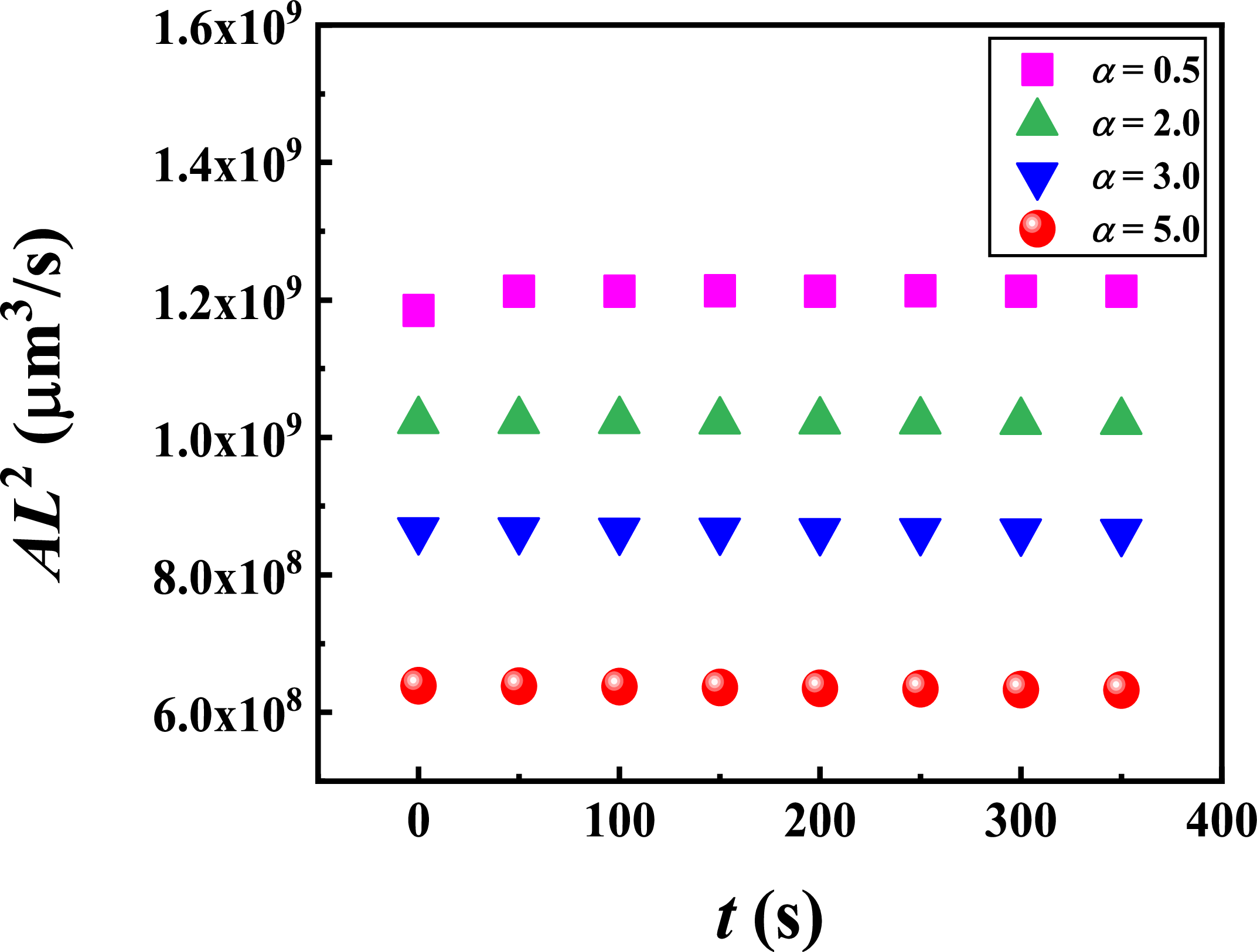
Dependence of the product of the maximum amplitude ( $A$
) and the square of the envelope width (
$A$
) and the square of the envelope width ( $L^2$
) as a function of time
$L^2$
) as a function of time $t$
for different
$t$
for different $\alpha$
, as given by (3.2). The horizontal axis represents time
$\alpha$
, as given by (3.2). The horizontal axis represents time $t$
(s), and the vertical axis represents
$t$
(s), and the vertical axis represents $A L^2$
(
$A L^2$
( $\unicode{x03BC} \mathrm{m}^3$
s−1). Different colours correspond to different
$\unicode{x03BC} \mathrm{m}^3$
s−1). Different colours correspond to different $\alpha$
values:
$\alpha$
values: $\alpha = 0.5$
,
$\alpha = 0.5$
, $2.0$
,
$2.0$
, $3.0$
and
$3.0$
and $5.0$
.
$5.0$
.

To further verify the soliton characteristics, apart from demonstrating the head-on collision between two envelope waves, figure 4 reveals that the product of the maximum amplitude $A$
and the square of the envelope width
$A$
and the square of the envelope width $L^2$
remains nearly constant with time for different
$L^2$
remains nearly constant with time for different $\alpha$
. The results show that, for different
$\alpha$
. The results show that, for different $\alpha$
values, the product of the envelope amplitude
$\alpha$
values, the product of the envelope amplitude $A$
and the square of its width
$A$
and the square of its width $L^2$
remains constant during the entire evolution process. This invariance is consistent with previous studies (Dharodi, Kumar & Sen Reference Dharodi, Kumar and Sen2023; Kumar et al. Reference Kumar, Bandyopadhyay, Singh and Sen2024).
$L^2$
remains constant during the entire evolution process. This invariance is consistent with previous studies (Dharodi, Kumar & Sen Reference Dharodi, Kumar and Sen2023; Kumar et al. Reference Kumar, Bandyopadhyay, Singh and Sen2024).
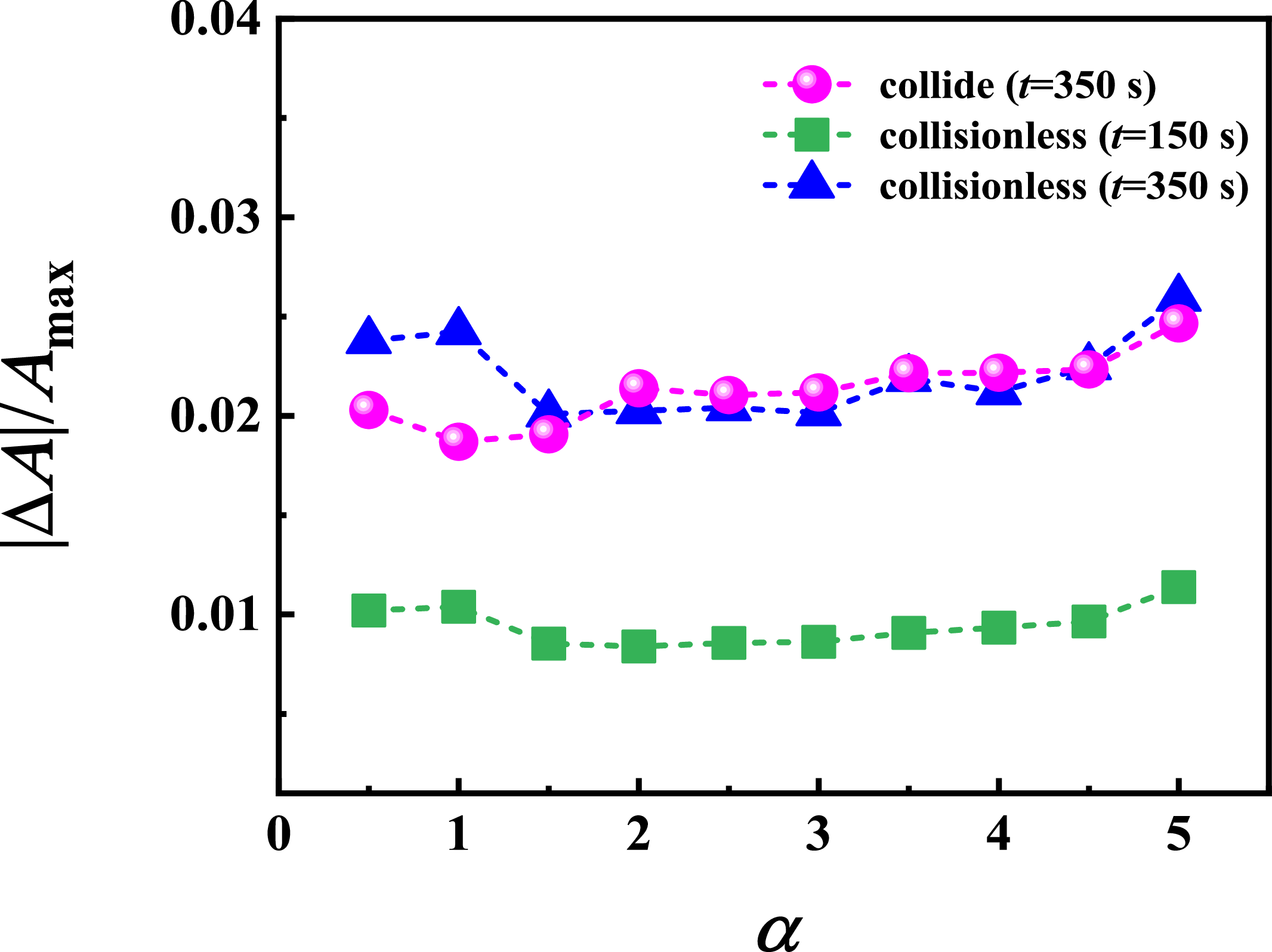
Relative error between the analytical and numerical results of the envelope wave at $t = 150$
s and
$t = 150$
s and $t = 350$
s varies with the parameter
$t = 350$
s varies with the parameter $\alpha$
. The relative error is defined as
$\alpha$
. The relative error is defined as $|\Delta A|/A_{\max }$
, where
$|\Delta A|/A_{\max }$
, where $\Delta A$
denotes the mean difference between the numerical and analytical velocities of each dust particle, and
$\Delta A$
denotes the mean difference between the numerical and analytical velocities of each dust particle, and $A_{\max }$
refers to the maximum amplitude of the envelope wave at the initial moment. Magenta circles indicate the relative error at
$A_{\max }$
refers to the maximum amplitude of the envelope wave at the initial moment. Magenta circles indicate the relative error at $t = 350$
s under collision conditions, green squares represent the error at
$t = 350$
s under collision conditions, green squares represent the error at $t = 150$
s without collision and blue triangles denote the error at
$t = 150$
s without collision and blue triangles denote the error at $t = 350$
s without collision.
$t = 350$
s without collision.

To quantitatively evaluate the consistency between the numerical simulations and the analytical results from (3.2) for the constructed envelope waves, we next examine the relative error as a function of the parameter $\alpha$
. Figure 5 presents the variation of the relative error
$\alpha$
. Figure 5 presents the variation of the relative error $|\Delta A| / A_{\text{max}}$
between the numerical and analytical results for envelope waves as a function of the parameter
$|\Delta A| / A_{\text{max}}$
between the numerical and analytical results for envelope waves as a function of the parameter $\alpha$
, evaluated at times
$\alpha$
, evaluated at times $t = 150$
s and
$t = 150$
s and $t = 350$
s, where
$t = 350$
s, where $\Delta A$
denotes the mean difference between the numerical and the analytical velocities of each dust particle derived from (3.2), and
$\Delta A$
denotes the mean difference between the numerical and the analytical velocities of each dust particle derived from (3.2), and $A_{\max }$
refers to the maximum amplitude of the envelope wave at the initial moment. The error is shown for both collisionless conditions (green squares and blue triangles) and collision conditions (magenta circles). The results reveal that the relative error increases with
$A_{\max }$
refers to the maximum amplitude of the envelope wave at the initial moment. The error is shown for both collisionless conditions (green squares and blue triangles) and collision conditions (magenta circles). The results reveal that the relative error increases with $\alpha$
, particularly in the collision scenarios. This increase is attributed to the enhanced nonlinear effects, which cause wavefront steepening and larger deviations from the theoretical results as
$\alpha$
, particularly in the collision scenarios. This increase is attributed to the enhanced nonlinear effects, which cause wavefront steepening and larger deviations from the theoretical results as $\alpha$
increases. The increasing relative error with
$\alpha$
increases. The increasing relative error with $\alpha$
reflects the growing impact of nonlinearity, which steepens the soliton wavefront. As a result, the simulation accuracy decreases due to larger deviations from the analytical results, demonstrating the sensitivity of the system to nonlinear effects.
$\alpha$
reflects the growing impact of nonlinearity, which steepens the soliton wavefront. As a result, the simulation accuracy decreases due to larger deviations from the analytical results, demonstrating the sensitivity of the system to nonlinear effects.
3.2. Propagation dynamics of a general wave
Section 3.1 verifies the existence of the envelope wave represented by (3.2) in the system. We now proceed to examine whether a more general initial wave condition can stably evolve in the system, For this purpose, we assume that there is a wave which satisfy the following equation:
 \begin{equation} s_i = \begin{cases} A \cos \left [k(x - x_0) - \omega t\right ] e^{\alpha (x - x_1)}, & 0 \leqslant x \lt x_1, \\ A \cos \left [k(x - x_0) - \omega t\right ], & x_1 \leqslant x \lt x_2, \\ A \cos \left [k(x - x_0) - \omega t\right ] e^{-\alpha (x - x_2)}, & x_2 \leqslant x .\end{cases} \end{equation}
Suppose that there are two waves. One is propagating in the positive $x$
direction (
$x$
direction ( $\omega \gt 0$
), while the other is in the negative
$\omega \gt 0$
), while the other is in the negative $x$
direction (
$x$
direction ( $\omega \lt 0$
).
$\omega \lt 0$
).
The initial position is set as $x_0 = 10$
,
$x_0 = 10$
, $\Delta x = x_2 - x_1 = 0.5$
, where
$\Delta x = x_2 - x_1 = 0.5$
, where $\omega$
satisfies the dispersion relation. The total number of dust particles is set to
$\omega$
satisfies the dispersion relation. The total number of dust particles is set to $N = 45\,000$
. The initial displacements and velocities of all particles are calculated from (3.5) and its time derivative.
$N = 45\,000$
. The initial displacements and velocities of all particles are calculated from (3.5) and its time derivative.
Comparison between the MD simulation results of waves in a one-dimensional dusty particle chain under different parameters: (a1–a3) $\alpha = 0.8$
; (b1–b3)
$\alpha = 0.8$
; (b1–b3) $\alpha = 2.0$
; (c1–c3)
$\alpha = 2.0$
; (c1–c3) $\alpha = 5.0$
) and at different times (
$\alpha = 5.0$
) and at different times ( $t = 200$
s and
$t = 200$
s and $t = 490$
s), with the initial waveform at
$t = 490$
s), with the initial waveform at $t = 0$
s, which is given by (3.5). The waveform at the initial time is represented by blue solid lines, while the numerical ones are expressed by magenta dots.
$t = 0$
s, which is given by (3.5). The waveform at the initial time is represented by blue solid lines, while the numerical ones are expressed by magenta dots.

Head-on collision of two waves in a one-dimensional dusty plasma chain with different parameters $\alpha$
at
$\alpha$
at $t = 0$
s,
$t = 0$
s, $290$
s and
$290$
s and $490$
s, which is given by (3.5). (a1–a3) Collision for
$490$
s, which is given by (3.5). (a1–a3) Collision for $\alpha = 1.4$
and
$\alpha = 1.4$
and $\alpha = 2.6$
, and (b1–b3) results for
$\alpha = 2.6$
, and (b1–b3) results for $\alpha = 5.0$
and
$\alpha = 5.0$
and $\alpha = 2.6$
. The waveform at the initial time is represented by blue solid lines, while the numerical ones are expressed by magenta dots.
$\alpha = 2.6$
. The waveform at the initial time is represented by blue solid lines, while the numerical ones are expressed by magenta dots.

Figure 6 presents the temporal evolution of an initial perturbation wave in a one-dimensional dusty plasma chain under different parameters $\alpha = 0.8$
,
$\alpha = 0.8$
, $2.0$
and
$2.0$
and $5.0$
, which is given by (3.5). The waveforms at
$5.0$
, which is given by (3.5). The waveforms at $t = 200$
s and
$t = 200$
s and $t = 490$
s are compared with that at
$t = 490$
s are compared with that at $t = 0$
s, showing the evolution of the solitary waves. Notice that with increasing
$t = 0$
s, showing the evolution of the solitary waves. Notice that with increasing $\alpha$
, the wave experiences more pronounced steepening and deviation from its initial symmetric cosine shape. Particularly, higher
$\alpha$
, the wave experiences more pronounced steepening and deviation from its initial symmetric cosine shape. Particularly, higher $\alpha$
leads to faster amplitude modulation and more evident wavefront distortion, indicating that the nonlinearity critically controls the dispersive and modulational characteristics of the evolving wave structure.
$\alpha$
leads to faster amplitude modulation and more evident wavefront distortion, indicating that the nonlinearity critically controls the dispersive and modulational characteristics of the evolving wave structure.
Figure 7 displays the evolution of head-on collision between two waves in a one-dimensional dusty plasma chain under different nonlinear parameters $\alpha$
. Figure 7(a1–a3) depicts the case of
$\alpha$
. Figure 7(a1–a3) depicts the case of $\alpha =1.4$
and
$\alpha =1.4$
and $\alpha =2.6$
, while figure 7(b1–b3) corresponds to
$\alpha =2.6$
, while figure 7(b1–b3) corresponds to $\alpha =5.0$
and
$\alpha =5.0$
and $\alpha =2.6$
. The velocity profiles are shown at
$\alpha =2.6$
. The velocity profiles are shown at $t = 0$
,
$t = 0$
, $180$
and
$180$
and $490$
s. After collision, the waves retain their general form, but exhibit minor amplitude fluctuations and phase shifts, especially for larger
$490$
s. After collision, the waves retain their general form, but exhibit minor amplitude fluctuations and phase shifts, especially for larger $\alpha$
. The results indicate that the interaction is weakly nonlinear and mostly elastic, with
$\alpha$
. The results indicate that the interaction is weakly nonlinear and mostly elastic, with $\alpha$
influencing the post-collision waveform fidelity. The nonlinear parameter
$\alpha$
influencing the post-collision waveform fidelity. The nonlinear parameter $\alpha$
modulates the balance between nonlinearity and dispersion, affecting wavefront steepness.
$\alpha$
modulates the balance between nonlinearity and dispersion, affecting wavefront steepness.
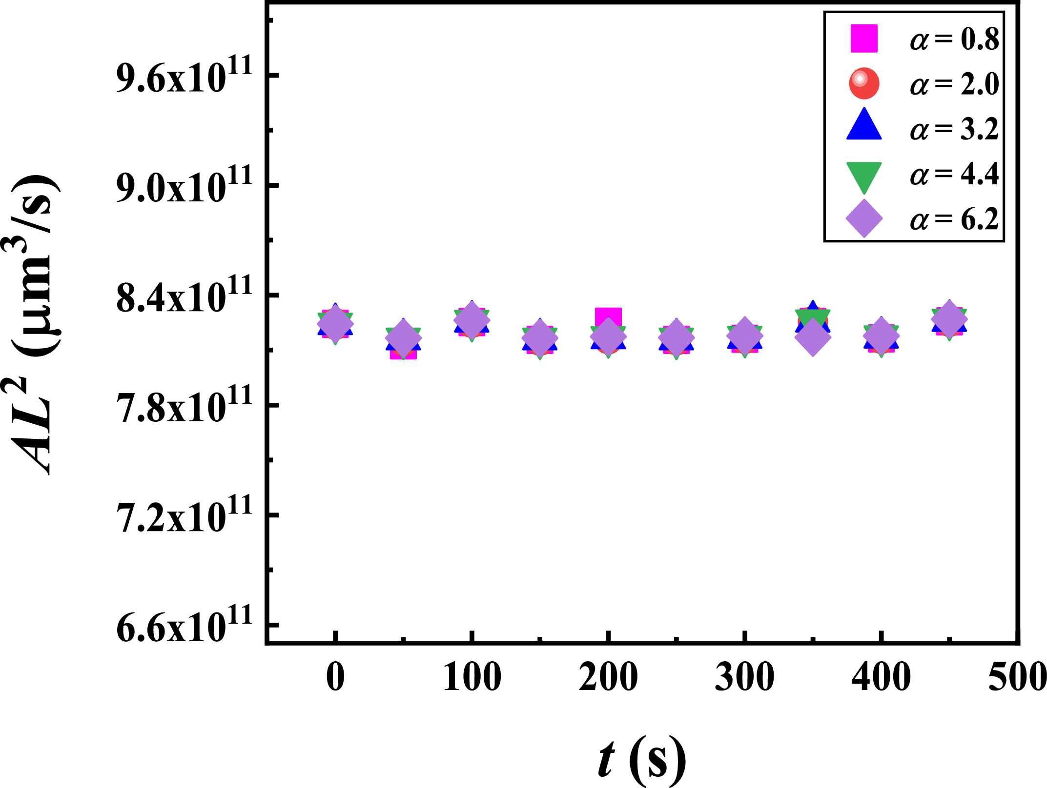
Figure 8 reveals that, for the wave described by (3.5), the product of the maximum amplitude $A$
and the square of the wave width
$A$
and the square of the wave width $L^2$
remains nearly constant with time for different
$L^2$
remains nearly constant with time for different $\alpha$
. This result demonstrates that the amplitude–width product is preserved throughout the entire evolution process, indicating robust soliton-like behaviour. This invariance is consistent with previous studies (Dharodi et al. Reference Dharodi, Kumar and Sen2023; Kumar et al. Reference Kumar, Bandyopadhyay, Singh and Sen2024).
$\alpha$
. This result demonstrates that the amplitude–width product is preserved throughout the entire evolution process, indicating robust soliton-like behaviour. This invariance is consistent with previous studies (Dharodi et al. Reference Dharodi, Kumar and Sen2023; Kumar et al. Reference Kumar, Bandyopadhyay, Singh and Sen2024).
Dependence of the product of the maximum amplitude ( $A$
) and the square of the wave width (
$A$
) and the square of the wave width ( $L^2$
) as a function of time
$L^2$
) as a function of time $t$
for different
$t$
for different $\alpha$
, as given by (3.5). The horizontal axis represents time
$\alpha$
, as given by (3.5). The horizontal axis represents time $t$
(s) and the vertical axis represents
$t$
(s) and the vertical axis represents $A L^2$
(
$A L^2$
( $\unicode{x03BC} \mathrm{m}^3$
s−1). Different colours correspond to different
$\unicode{x03BC} \mathrm{m}^3$
s−1). Different colours correspond to different $\alpha$
values:
$\alpha$
values: $\alpha = 0.8$
,
$\alpha = 0.8$
, $2.0$
,
$2.0$
, $3.2$
,
$3.2$
, $4.4$
and
$4.4$
and $6.2$
.
$6.2$
.

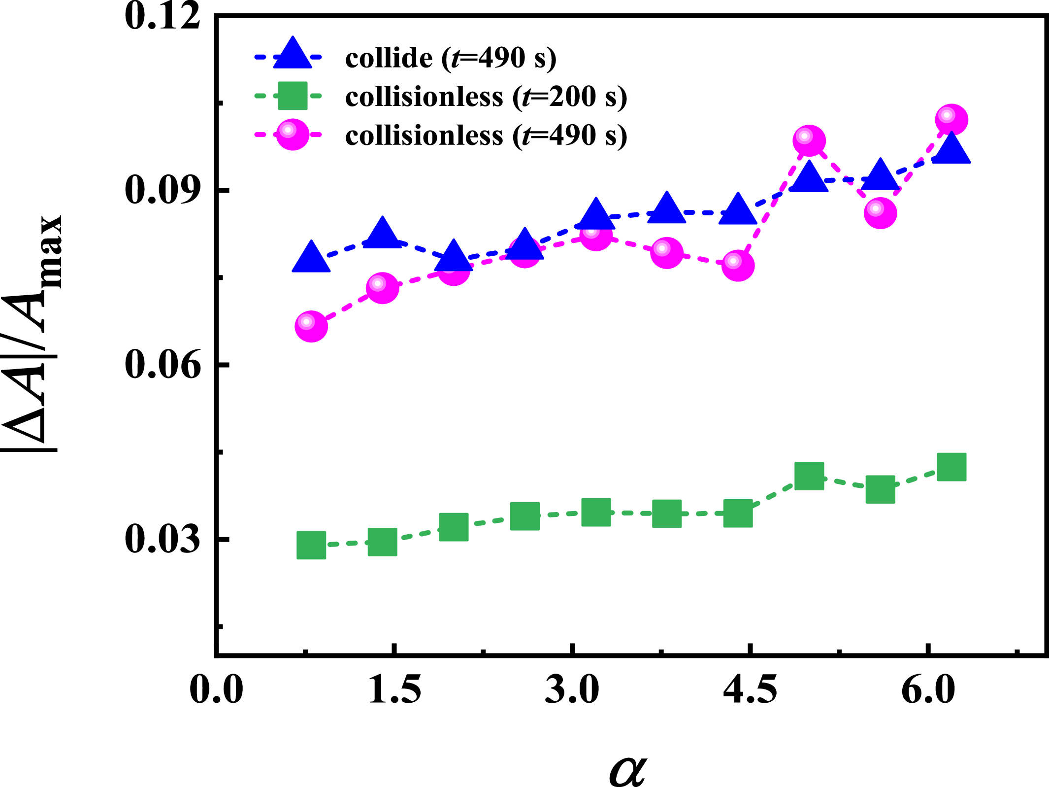
Variation of the relative error $|\Delta A|/A_{\max }$
between the numerical results of the wave obtained from (3.5) at
$|\Delta A|/A_{\max }$
between the numerical results of the wave obtained from (3.5) at $t = 200$
s and
$t = 200$
s and $t = 490$
s, and the initial waveform, with respect to the parameter
$t = 490$
s, and the initial waveform, with respect to the parameter $\alpha$
. The relative error is defined as
$\alpha$
. The relative error is defined as $|\Delta A|/A_{\max }$
, where
$|\Delta A|/A_{\max }$
, where $\Delta A$
represents the mean difference between the velocity of each dust particle and the initial time at different times, and
$\Delta A$
represents the mean difference between the velocity of each dust particle and the initial time at different times, and $A_{\max }$
is the maximum amplitude of the wave at the initial time. Blue triangles represent the error at
$A_{\max }$
is the maximum amplitude of the wave at the initial time. Blue triangles represent the error at $t=490$
s under collision conditions, magenta circles denote the relative error at
$t=490$
s under collision conditions, magenta circles denote the relative error at $t=490$
s without collision and green squares indicate the error at
$t=490$
s without collision and green squares indicate the error at $t=200$
s without collision.
$t=200$
s without collision.

Figure 9 illustrates the variation of the relative error of the wave described by (3.5) at $t = 200$
s and
$t = 200$
s and $t = 490$
s with respect to the nonlinear parameter
$t = 490$
s with respect to the nonlinear parameter $\alpha$
. The relative error is defined as
$\alpha$
. The relative error is defined as $|\Delta A|/A_{\max }$
. As
$|\Delta A|/A_{\max }$
. As $\alpha$
increases, the relative error also increases, particularly at later times. This suggests that higher values of
$\alpha$
increases, the relative error also increases, particularly at later times. This suggests that higher values of $\alpha$
lead to greater nonlinearity, which causes deviations from the initial waveform. The increasing relative error with
$\alpha$
lead to greater nonlinearity, which causes deviations from the initial waveform. The increasing relative error with $\alpha$
reflects the enhanced nonlinearity, which causes wavefront steepening and amplifies deviations from the analytical solution slightly. These findings offer guidance for minimising errors in simulation, which improves wave propagation modelling, and in dusty plasma experiments.
$\alpha$
reflects the enhanced nonlinearity, which causes wavefront steepening and amplifies deviations from the analytical solution slightly. These findings offer guidance for minimising errors in simulation, which improves wave propagation modelling, and in dusty plasma experiments.
4. Conclusion
This study investigates the existence, stability and interaction of non-standard envelope waves in one-dimensional dusty plasma chains. The results in the present paper are consistent with those in the previously reported ones, which studied the standard envelope solitons in dusty plasmas (Zhang et al. Reference Zhang, Qi, Duan and Yang2015; Rahman et al. Reference Rahman, Chowdhury, Mannan, Rahman and Mamun2018; Houwe et al. Reference Houwe, Abbagari, Inc, Betchewe, Doka and Crépin2022). By combining analytical derivation using the NLSE and MD simulations, we verify the stable propagation of artificially modulated envelope solitons, even beyond the standard NLSE framework. Notably, envelope waves with varying widths maintain structural integrity and display elastic-like collisions, demonstrating soliton-like characteristics. These findings answer the paper’s initial question regarding the existence and stability of arbitrary envelope waveforms in dusty plasma lattices, significantly extending prior work limited to analytical NLSE solutions.
The paper’s primary contribution is demonstrating the stable existence and elastic-like collision of non-standard envelope waves in dusty plasma chains using MD simulations beyond conventional NLSE solitons. It introduces $\alpha$
as a tuneable parameter for envelope shaping and confirms robustness through precise error analysis. Crucially, it reveals that such envelope structures remain stable even when initially asymmetric, enriching the theoretical and practical understanding of nonlinear wave phenomena. This enables controlled waveform design in plasma-based applications, a novel insight for future experimental manipulation. The study advances nonlinear plasma physics by enabling customisable, stable waveform design for dusty plasmas.
$\alpha$
as a tuneable parameter for envelope shaping and confirms robustness through precise error analysis. Crucially, it reveals that such envelope structures remain stable even when initially asymmetric, enriching the theoretical and practical understanding of nonlinear wave phenomena. This enables controlled waveform design in plasma-based applications, a novel insight for future experimental manipulation. The study advances nonlinear plasma physics by enabling customisable, stable waveform design for dusty plasmas.
Acknowledgements
The numerical calculations in this paper have been done on the supercomputing system in the Dongjiang Yuan Intelligent Computing Center.
Editor Edward Thomas, Jr. thanks the referees for their advice in evaluating this article.
Funding
This work was supported by the National Natural Science Foundation of China No. 12275223, the Gansu National Natural Science Foundation (24JRRP004) and the Innovation Fund for University Teachers in Gansu Province (2025A-212).
Declaration of interests
The authors report no conflicts of interest.
Data availability statement
The data that support the findings of this study are available within the article.
Appendix A. Reductive perturbation method for obtaining the first three powers of
$\varepsilon$
.

Here, we provide a detailed exposition of the key mathematical steps involved in the reductive perturbation method for obtaining the first three powers of $\varepsilon$
. The quantity of
$\varepsilon$
. The quantity of $\xi$
is expanded as (Gao et al. Reference Gao, Zhang, Zhang, Li and Duan2017; Lee Reference Lee2010; Veeresha et al. Reference Veeresha, Tiwari, Sen, Kaw and Das2010; Bala, Gill & Kaur Reference Bala, Gill and Kaur2012; Shalini & Misra Reference Shalini and Misra2015)
$\xi$
is expanded as (Gao et al. Reference Gao, Zhang, Zhang, Li and Duan2017; Lee Reference Lee2010; Veeresha et al. Reference Veeresha, Tiwari, Sen, Kaw and Das2010; Bala, Gill & Kaur Reference Bala, Gill and Kaur2012; Shalini & Misra Reference Shalini and Misra2015)
 \begin{equation} \xi = \sum _{n=1}^\infty \varepsilon ^n \sum _{l=-\infty }^{+\infty }\xi ^{(n,l)}(\eta , \tau )e^{il(kx-\omega t)}. \end{equation}
By substituting these expansions into (2.1), we obtain the following equations corresponding to different orders of $\varepsilon$
. At
$\varepsilon$
. At $\varepsilon$
, we have
$\varepsilon$
, we have
 \begin{align} - l^2 \omega ^2 \sum \limits _{l = -\infty }^{+\infty } \xi ^{(1,l)} e^{i l (k x - \omega t)} = B_1\Bigg[\!- l^2 k^2 \sum \limits _{l = -\infty }^{+\infty } \xi ^{(1,l)} e^{i l (k x - \omega t)} + \frac {a_0^2}{12} l^4 k^4 \sum \limits _{l = -\infty }^{+\infty } \xi ^{(1,l)} e^{i l (k x - \omega t)} \Bigg ].\nonumber\\[2pt] \end{align}
For $l$
= 1, we can obtain the dispersion relation:
$l$
= 1, we can obtain the dispersion relation: $\omega ^2= B_1k^2[1-{(a_0^2 / 12)} k^2]$
.
$\omega ^2= B_1k^2[1-{(a_0^2 / 12)} k^2]$
.
At $\varepsilon ^2$
,
$\varepsilon ^2$
,
 \begin{align} &2il\omega V\sum \limits _{l = - \infty }^{ + \infty } {\frac {{\partial {\xi ^{\left ( {1,l} \right )}}}}{{\partial \eta }}{e^{il(kx - \omega t)}}} - {l^2}{\omega ^2}\sum \limits _{l = - \infty }^{ + \infty } {{\xi ^{\left ( {2,l} \right )}}}{e^{il(kx - \omega t)}} \nonumber \\ &\quad = {B_1}\left [ {2ilk\sum \limits _{l = - \infty }^{ + \infty } {\frac {{\partial {\xi ^{\left ( {1,l} \right )}}}}{{\partial \eta }}{e^{il(kx - \omega t)}} - {l^2}{k^2}\sum \limits _{l = - \infty }^{ + \infty } {{\xi ^{\left ( {2,l} \right )}}{e^{il(kx - \omega t)}}} } } \right ] \nonumber \\&\qquad + \frac {{a_0^2}}{{12}}{B_1}\left [ {{l^4}{k^4}{\xi ^{\left ( {2,l} \right )}}{e^{il(kx - \omega t)}} - 4i{l^3}{k^3}\sum \limits _{l = - \infty }^{ + \infty } {\frac {{\partial {\xi ^{\left ( {1,l} \right )}}}}{{\partial \eta }}{e^{il(kx - \omega t)}}} } \right ] \nonumber \\&\qquad - {B_2}ilk\sum \limits _{l = - \infty }^{ + \infty } {{\xi ^{\left ( {1,l} \right )}}} {e^{il(kx - \omega t)}}{l^2}{k^2}\sum \limits _{l = - \infty }^{ + \infty } {{\xi ^{\left ( {1,l} \right )}}} {e^{il(kx - \omega t)}}. \end{align}
For $l$
= 1, we can obtain the group velocity:
$l$
= 1, we can obtain the group velocity: $V= B_1{(k / \omega) }[1-{(a_0^2 / 6)} k^2]$
.
$V= B_1{(k / \omega) }[1-{(a_0^2 / 6)} k^2]$
.
At $\varepsilon ^3$
,
$\varepsilon ^3$
,
 \begin{eqnarray} &&V^2 \sum \limits _{l = - \infty }^{ + \infty }\frac {\partial ^2 \xi ^{(1,l)}}{\partial \eta ^2} e^{il(kx - \omega t)} + 2 i l \omega V \sum \limits _{l = - \infty }^{ + \infty }\frac {\partial \xi ^{(2,l)}}{\partial \eta } e^{il(kx - \omega t)} - 2 i l \omega \sum \limits _{l = - \infty }^{ + \infty } \frac {\partial \xi ^{(1,l)}}{\partial \tau } e^{il(kx - \omega t)} \nonumber \\&&-\ l^2 \omega ^2 \sum \limits _{l = - \infty }^{ + \infty } \xi ^{(3,l)} e^{il(kx - \omega t)}= B_1 \Bigg [ \sum \limits _{l = - \infty }^{ + \infty } \frac {\partial ^2 \xi ^{(1,l)}}{\partial \eta ^2} \, e^{i l (k x - \omega t)} + 2 i l k \sum \limits _{l = - \infty }^{ + \infty } \frac {\partial \xi ^{(2,l)}}{\partial \eta } \, e^{i l (k x - \omega t)} \nonumber\\&&-\ l^2 k^2 \sum \limits _{l = - \infty }^{ + \infty } \xi ^{(3,l)} \, e^{i l (k x - \omega t)}\! \Bigg ]+ \frac {a_0^2}{12} B_1 \Bigg [\! {-} 6 l^2 k^2 \sum \limits _{l = - \infty }^{ + \infty } \frac {\partial ^2 \xi ^{(1,l)}}{\partial \eta ^2} \, e^{i l (k x - \omega t)} - 4 i l^3 k^3 \sum \limits _{l = - \infty }^{ + \infty } \frac {\partial \xi ^{(2,l)}}{\partial \eta } \, \nonumber\\&&\times\ e^{i l (k x - \omega t)} + l^4 k^4 \sum \limits _{l = - \infty }^{ + \infty } \xi ^{(3,l)} \, e^{i l (k x - \omega t)} \Bigg ] + B_2 \Bigg [ i l k \sum \limits _{l = - \infty }^{ + \infty } \xi ^{(1,l)} \, e^{i l (k x - \omega t)} 2 i l k \sum \limits _{l = - \infty }^{ + \infty } \frac {\partial \xi ^{(1,l)}}{\partial \eta } \, \nonumber\\ &&\times\ e^{i l (k x - \omega t)} - i l k \sum \limits _{l = - \infty }^{ + \infty } \xi ^{(1,l)} \, e^{i l (k x - \omega t)} l^2 k^2 \sum \limits _{l = - \infty }^{ + \infty } \xi ^{(2,l)} \, e^{i l (k x - \omega t)} - \sum \limits _{l = - \infty }^{ + \infty } \frac {\partial \xi ^{(1,l)}}{\partial \eta } \, e^{i l (k x - \omega t)} \, \nonumber \\&&\times\ l^2 k^2 \sum \limits _{l = - \infty }^{ + \infty } \xi ^{(1,l)} \, e^{i l (k x - \omega t)} - i l k \sum \limits _{l = - \infty }^{ + \infty } \xi ^{(2,l)} \, e^{i l (k x - \omega t)} \, l^2 k^2 \sum \limits _{l = - \infty }^{ + \infty } \xi ^{(1,l)} \, e^{i l (k x - \omega t)}\Bigg ]. \end{eqnarray}
By simplification, we can obtain the NLSE:
 \begin{equation} i{\frac{\partial \xi ^{(1,1)} }{ \partial \tau }} +P{\frac{\partial ^2 \xi ^{(1,1)}}{ \partial \eta ^2 }} +Q\xi ^{(1,1)}\mid \xi ^{(1,1)}\mid ^2 =0, \end{equation}
where $P = ({{2{B_1} - 2{V^2} - {B_1}a_0^2{k^2}}}/{{4\omega }})$
,
$P = ({{2{B_1} - 2{V^2} - {B_1}a_0^2{k^2}}}/{{4\omega }})$
, $Q=({3 B_2^2 k^6 / -12\omega ^3+12\omega k^2 B_1-4\omega B_1 a_0^2 k^4})$
.
$Q=({3 B_2^2 k^6 / -12\omega ^3+12\omega k^2 B_1-4\omega B_1 a_0^2 k^4})$
.












 Open access

