


1. Introduction
Predicting the intricate dynamics of solute movement and mass transport within porous materials is essential across a variety of natural and engineered processes, including agriculture, chemical engineering, biology and a myriad application areas related to the energy sector (Sahimi Reference Sahimi1993; Lima et al. Reference Lima, Ishikawa, Imai, Takeda, Wada and Yamaguchi2008; Bijeljic et al. Reference Bijeljic, Raeini, Mostaghimi and Blunt2013; Baioni et al. Reference Baioni, Mousavi Nezhad, Porta and Guadagnini2021). However, this task is often challenging due to the inherent variability of porous media and complex interactions between fluids and the solid porous geometry that can lead to anomalous dispersion behaviours, where the spreading of solutes deviates significantly from classical diffusion models (Capuani, Frenkel & Lowe Reference Capuani, Frenkel and Lowe2003; Zhang et al. Reference Zhang, Suekane, Minokawa, Hu and Patmonoaji2019). This becomes even more critical when non-Newtonian fluids are involved, as their complex rheological behaviour can significantly influence flow and transport processes, even at low Reynolds numbers (Rodriguez de Castro & Radilla Reference Rodriguez de Castro and Radilla2017; Ekanem et al. Reference Ekanem, Berg, De, Fadili, Bultreys, Rücker, Southwick, Crawshaw and Luckham2020; An et al. Reference An, Sahimi and Niasar2022), $\textit {Re} = \rho uL/\eta \lesssim 100$
, where
$\textit {Re} = \rho uL/\eta \lesssim 100$
, where $\rho$
is the density the Newtonian solvent,
$\rho$
is the density the Newtonian solvent, $u$
is the pore velocity,
$u$
is the pore velocity, $L$
is the characteristic length and
$L$
is the characteristic length and $\eta$
is the dynamic viscosity of the fluid.
$\eta$
is the dynamic viscosity of the fluid.
The literature on the interactions between the flow and the solid porous geometry has been primarily focused on Newtonian fluids. Experimental observations have revealed that chaotic mixing mechanisms driven by grain contacts significantly enhance concentration gradients, challenging traditional dispersion models that average pore-scale fluctuations (Heyman et al. Reference Heyman, Lester, Turuban, Méheust and Le Borgne2020). Bijeljic & Blunt (Reference Bijeljic and Blunt2007) investigated the transverse dispersion coefficient ( $D_{\perp }$
) in porous media utilising a pore-network model to simulate solute transport across a spectrum of Péclet number (
$D_{\perp }$
) in porous media utilising a pore-network model to simulate solute transport across a spectrum of Péclet number ( $Pe$
, the ratio of advection to diffusion rates) values ranging from 0 to 10
$Pe$
, the ratio of advection to diffusion rates) values ranging from 0 to 10 $^5$
. Bijeljic & Blunt (Reference Bijeljic and Blunt2007) established that
$^5$
. Bijeljic & Blunt (Reference Bijeljic and Blunt2007) established that $D_{\perp }$
scales approximately linearly with
$D_{\perp }$
scales approximately linearly with $Pe\gg 1$
and identified four distinct dispersion regimes: restricted diffusion, transition, power law and mechanical dispersion. This highlights the substantial influence of the pore size distribution and network orientation on dispersion behaviour, and suggests that the assumption of a fixed ratio between the transverse and longitudinal dispersion coefficients
$Pe\gg 1$
and identified four distinct dispersion regimes: restricted diffusion, transition, power law and mechanical dispersion. This highlights the substantial influence of the pore size distribution and network orientation on dispersion behaviour, and suggests that the assumption of a fixed ratio between the transverse and longitudinal dispersion coefficients $D_{\parallel }/D_{\perp }$
is inappropriate outside the advection-dominated regime. Meigel et al. (Reference Meigel, Darwent, Bastin, Goehring and Alim2022) demonstrated a non-monotonic relationship between transport efficiency and pore space heterogeneity, revealing that transport efficiency initially increased with the disorder before decreasing at higher levels of heterogeneity.
$D_{\parallel }/D_{\perp }$
is inappropriate outside the advection-dominated regime. Meigel et al. (Reference Meigel, Darwent, Bastin, Goehring and Alim2022) demonstrated a non-monotonic relationship between transport efficiency and pore space heterogeneity, revealing that transport efficiency initially increased with the disorder before decreasing at higher levels of heterogeneity.
Non-Newtonian features, including nonlinear rheology and elastic instabilities, further compound these complex interactions between the flow and the porous geometry in porous medium fluid flows. For instance, the pressure drop and flow resistance in porous media are influenced by both the mean flow and local velocity fluctuations arising due to elastic instabilities, particularly when elastic stresses are larger than viscous stresses, characterised by higher Weissenberg ( $Wi\gg 1$
) numbers, which quantify the ratio of elastic to viscous stresses (Haward, Hopkins & Shen Reference Haward, Hopkins and Shen2021; Ibezim, Dennis & Poole Reference Ibezim, Dennis and Poole2024). The complex interactions between elastic instabilities and porous geometries are known to lead to chaotic flow behaviour (Dzanic et al. Reference Dzanic, From, Gupta, Xie and Sauret2023). Such chaotic flow generated by elastic instabilities has recently been shown to enhance mixing and reaction kinetics in porous media with the addition of flexible polymers, significantly reducing the mixing length required for effective solute dispersion, thus improving the efficiency of chemical reactions (Browne & Datta Reference Browne and Datta2024). Numerical simulations have revealed the complex behaviour of dispersive transport in porous media with non-Newtonian fluids at high Péclet numbers to be influenced by fluid properties (Cheng et al. Reference Cheng, Lien, Zhang and Gu2024). One example is the emergence of diffusion (blind) zones, where solute transport is notably restricted. Cheng et al. (Reference Cheng, Lien, Zhang and Gu2024) observed that higher injection velocities give rise to circumferential flow patterns and the formation of twin vortices, which contribute to incomplete solute dispersion by reinforcing these hindered zones.
$Wi\gg 1$
) numbers, which quantify the ratio of elastic to viscous stresses (Haward, Hopkins & Shen Reference Haward, Hopkins and Shen2021; Ibezim, Dennis & Poole Reference Ibezim, Dennis and Poole2024). The complex interactions between elastic instabilities and porous geometries are known to lead to chaotic flow behaviour (Dzanic et al. Reference Dzanic, From, Gupta, Xie and Sauret2023). Such chaotic flow generated by elastic instabilities has recently been shown to enhance mixing and reaction kinetics in porous media with the addition of flexible polymers, significantly reducing the mixing length required for effective solute dispersion, thus improving the efficiency of chemical reactions (Browne & Datta Reference Browne and Datta2024). Numerical simulations have revealed the complex behaviour of dispersive transport in porous media with non-Newtonian fluids at high Péclet numbers to be influenced by fluid properties (Cheng et al. Reference Cheng, Lien, Zhang and Gu2024). One example is the emergence of diffusion (blind) zones, where solute transport is notably restricted. Cheng et al. (Reference Cheng, Lien, Zhang and Gu2024) observed that higher injection velocities give rise to circumferential flow patterns and the formation of twin vortices, which contribute to incomplete solute dispersion by reinforcing these hindered zones.
Pore-scale flow visualisation in porous media has advanced considerably over the past decade through techniques such as micro-particle image velocimetry ( $\mu$
PIV), nanoparticle tracking and confocal microscopy. Several studies have demonstrated the capability of these methods to resolve velocity fields at the pore scale for Newtonian and non-Newtonian fluids. For example, Ibezim et al. (Reference Ibezim, Dennis and Poole2024) employed
$\mu$
PIV), nanoparticle tracking and confocal microscopy. Several studies have demonstrated the capability of these methods to resolve velocity fields at the pore scale for Newtonian and non-Newtonian fluids. For example, Ibezim et al. (Reference Ibezim, Dennis and Poole2024) employed $\mu$
PIV to examine viscoelastic polymer flow in a three-dimensional sintered-glass porous medium and reported the emergence of elastic instabilities and velocity fluctuations at elevated Weissenberg numbers. Similarly, Babayekhorasani et al. (Reference Babayekhorasani, Dunstan, Krishnamoorti and Conrad2016) used microfluidic channels to track individual nanoparticles in glycerol/water mixtures and Hydrolyzed polyacrylamide solutions, enabling estimates of dispersion and pore-scale velocity distributions. Beyond individual experiments, recent reviews, such as those by Datta et al. (Reference Datta2022), have synthesised recent advances in viscoelastic flow behaviour, elastic turbulence and complex rheological effects in porous media. In addition, Datta et al. (Reference Datta, Chiang, Ramakrishnan and Weitz2013) visualised Newtonian flow in a three-dimensional porous medium using confocal microscopy and revealed exponential velocity distributions and pore-scale correlations. Collectively, these studies show that direct visualisation of pore-scale flow is well established in the broader context of complex fluid transport.
$\mu$
PIV to examine viscoelastic polymer flow in a three-dimensional sintered-glass porous medium and reported the emergence of elastic instabilities and velocity fluctuations at elevated Weissenberg numbers. Similarly, Babayekhorasani et al. (Reference Babayekhorasani, Dunstan, Krishnamoorti and Conrad2016) used microfluidic channels to track individual nanoparticles in glycerol/water mixtures and Hydrolyzed polyacrylamide solutions, enabling estimates of dispersion and pore-scale velocity distributions. Beyond individual experiments, recent reviews, such as those by Datta et al. (Reference Datta2022), have synthesised recent advances in viscoelastic flow behaviour, elastic turbulence and complex rheological effects in porous media. In addition, Datta et al. (Reference Datta, Chiang, Ramakrishnan and Weitz2013) visualised Newtonian flow in a three-dimensional porous medium using confocal microscopy and revealed exponential velocity distributions and pore-scale correlations. Collectively, these studies show that direct visualisation of pore-scale flow is well established in the broader context of complex fluid transport.
In the absence of elastic instabilities, the intrinsic rheological properties of non-Newtonian fluids, in particular shear-thinning effects, have been experimentally observed to lead to an increased dispersion (D’Onofrio et al. Reference D’Onofrio, Freytes, Rosen, Allain and Hulin2002; Al-Qenae et al. Reference Al-Qenae, Shokri, Shende, Sahimi and Niasar2025), where recent numerical studies have suggested that the spatial variability of the shear-dependent viscosity of non-Newtonian shear-thinning fluids leads to this enhanced dispersion in contrast to traditional Newtonian fluids (An et al. Reference An, Sahimi and Niasar2022; Omrani et al. Reference Omrani, Green, Sahimi and Niasar2024). Experimental investigations by Seybold et al. (Reference Seybold2021) suggest that shear-thinning effects significantly influence flow patterns, leading to enhanced channelling and localisation effects; however, they did not experimentally measure dispersion. Recent numerical investigations by Omrani et al. (Reference Omrani, Green, Sahimi and Niasar2024) observed that dispersivity is a non-monotonic function of the Péclet number and shear rate, significantly influenced by the heterogeneity of the pore space, with which localised viscosity variations lead to variations in flow speeds, affecting how the solutes disperse (An et al. Reference An, Sahimi and Niasar2022).
Recent work by Al-Qenae et al. (Reference Al-Qenae, Shokri, Shende, Sahimi and Niasar2025) experimentally examined solute transport in a shear-thinning Xanthan gum solution through a porous micromodel with random pore geometry, using optical microscopy, revealing a non-monotonic relationship between dispersivity and injection rate, in contrast to the constant dispersivity typically observed in Newtonian fluids. To account for this variability, Al-Qenae et al. (Reference Al-Qenae, Shokri, Shende, Sahimi and Niasar2025) proposed a rheology-dependent correction factor for the dispersion coefficient, suggesting that this behaviour is attributed to spatial variability in the viscosity caused by the shear-thinning rheology, which alters the local velocity field and transport dynamics. However, the pore-scale velocity field was not measured directly, so the proposed mechanism, the variations in the velocity field induced by rheological effects and the impact on dispersivity, were only inferred indirectly; thus, direct experimental observation remains to be seen.
A similar non-monotonic transport response has been reported in other complex systems. For example, Kurzthaler et al. (Reference Kurzthaler, Mandal, Bhattacharjee, Löwen, Datta and Stone2021) demonstrated that the spreading of active polymer chains in porous media varies non-monotonically with their run length, arising from the interplay between persistent motion and geometric confinement. Although the physical mechanism in active polymer systems differs fundamentally from the shear-rate-dependent viscosity examined here, both cases illustrate how nonlinear coupling between the pore-scale dynamics and pore geometry can give rise to non-monotonic macroscopic transport behaviour.
Overall, the collective findings from these investigations highlight the importance of considering both the fluid’s rheological properties and the porous medium’s geometric characteristics in predicting and controlling flow behaviour in various applications accurately. Integrating theoretical models with experimental observations continues to advance our understanding of these complex systems. Non-destructive experimental visualisation methods are vital to this end (Nguyen, King & Hassan Reference Nguyen, King and Hassan2021), allowing observations of how fluids move and interact within porous materials to measure dispersion and mixing processes.
Recent research has effectively utilised various technologies such as optical microscopy, X-ray micro-Computed Tomography (micro-CT) and magnetic resonance imaging (MRI) to investigate dispersion behaviour at the pore scale (Boon et al. Reference Boon, Bijeljic, Niu and Krevor2016; Lehoux et al. Reference Lehoux, Rodts, Faure, Michel, Courtier-Murias and Coussot2016; Karadimitriou et al. Reference Karadimitriou, Joekar-Niasar, Babaei and Shore2016; Boon, Bijeljic & Krevor Reference Boon, Bijeljic and Krevor2017; Zhang et al. Reference Zhang, Suekane, Minokawa, Hu and Patmonoaji2019; Hasan et al. Reference Hasan, Niasar, Karadimitriou, Godinho, Vo, An, Rabbani and Steeb2020; Souzy et al. Reference Souzy, Lhuissier, Méheust, Le Borgne and Metzger2020; Chen et al. Reference Chen2021). While early applications of micro-CT and MRI primarily provided geometric or concentration information, recent methodological advances have enabled the reconstruction of three-dimensional pore-scale velocity fields using these volumetric imaging techniques (Karlsons et al. Reference Karlsons, De Kort, Sederman, Mantle, Freeman, Appel and Gladden2021; Bultreys et al. Reference Bultreys2024). Nevertheless, their spatial and temporal resolutions remain substantially lower than those achieved by optical microscopy combined with $\mu$
PIV, intensity mapping or refractive index matching, which provide high-fidelity measurements of the velocity, shear rate and mixing dynamics in quasi-two-dimensional micromodels (Beard Reference Beard2001; Datta & Ghosal Reference Datta and Ghosal2009; Capretto et al. Reference Capretto, Cheng, Hill and Zhang2011; Alijani et al. Reference Alijani, Özbey, Karimzadehkhouei and Koşar2019).
$\mu$
PIV, intensity mapping or refractive index matching, which provide high-fidelity measurements of the velocity, shear rate and mixing dynamics in quasi-two-dimensional micromodels (Beard Reference Beard2001; Datta & Ghosal Reference Datta and Ghosal2009; Capretto et al. Reference Capretto, Cheng, Hill and Zhang2011; Alijani et al. Reference Alijani, Özbey, Karimzadehkhouei and Koşar2019).
Despite these advances, a direct experimental quantification of how spatial variations in the local shear-dependent viscosity, arising specifically from a shear-thinning rheology, modify both the pore-scale velocity field and the resulting hydrodynamic dispersion has only been inferred indirectly, and has not yet been demonstrated. Prior work has focused mainly on viscoelastic instabilities, nanoparticle transport or Newtonian velocity statistics, without linking rheology-controlled viscosity heterogeneity to dispersion. In contrast, the present study investigates the flow of a shear-thinning Xanthan gum solution through a quasi-two-dimensional disordered porous micromodel under conditions where elasticity is negligible, and the flow remains steady.
We employ $\mu$
PIV to directly measure the pore-scale velocity, shear-rate and flow-type fields, and use these to: (i) compute the advection-diffusion scalar transport, (ii) compute the effective dispersion via two independent methods based on breakthrough curves, (iii) compute the components of the dispersion tensor directly from spatial methods of moments and (iv) test the hypothesised role of shear-viscosity-induced velocity heterogeneity.
$\mu$
PIV to directly measure the pore-scale velocity, shear-rate and flow-type fields, and use these to: (i) compute the advection-diffusion scalar transport, (ii) compute the effective dispersion via two independent methods based on breakthrough curves, (iii) compute the components of the dispersion tensor directly from spatial methods of moments and (iv) test the hypothesised role of shear-viscosity-induced velocity heterogeneity.
In this work, we investigate non-Newtonian shear-thinning fluid flow in an irregular porous medium comprising random pore geometry using $\mu$
PIV and compare the dispersion and fluid flow behaviour against the Newtonian analogue. Specifically, our research aims to understand the differences in the fluid dynamics at different Péclet numbers (
$\mu$
PIV and compare the dispersion and fluid flow behaviour against the Newtonian analogue. Specifically, our research aims to understand the differences in the fluid dynamics at different Péclet numbers ( $Pe$
) due to the shear-dependent viscosity of non-Newtonian fluid flows in porous media and their impact on dispersion. To the best of our knowledge, this study represents a notable advancement in our field, providing the first direct experimental observation of the velocity field and dispersion in non-Newtonian shear-thinning fluid flow through random porous media.
$Pe$
) due to the shear-dependent viscosity of non-Newtonian fluid flows in porous media and their impact on dispersion. To the best of our knowledge, this study represents a notable advancement in our field, providing the first direct experimental observation of the velocity field and dispersion in non-Newtonian shear-thinning fluid flow through random porous media.
2. Materials and methods
Building on our previous work (Al-Qenae et al. Reference Al-Qenae, Shokri, Shende, Sahimi and Niasar2025), we investigate how shear-dependent viscosity influences flow and dispersion behaviour in the same irregular porous medium (figure 2
b), focusing on how these effects vary with $Pe$
. Specifically, we aim to understand the differences in solute transport between Newtonian and shear-thinning fluids across a range of
$Pe$
. Specifically, we aim to understand the differences in solute transport between Newtonian and shear-thinning fluids across a range of $Pe$
, and whether the observed non-monotonicity in dispersivity arises from changes in the velocity field induced by rheological effects. By directly measuring the velocity field using
$Pe$
, and whether the observed non-monotonicity in dispersivity arises from changes in the velocity field induced by rheological effects. By directly measuring the velocity field using $\mu$
PIV experiments, we seek to gain further insight into how fluid rheology interacts with pore-scale heterogeneity to shape dispersion.
$\mu$
PIV experiments, we seek to gain further insight into how fluid rheology interacts with pore-scale heterogeneity to shape dispersion.
2.1. Experimental methods
This section outlines the preparation of fluids and the measurement of their rheological properties, followed by an overview of the experimental system, procedures and $\mu$
PIV used for measurement.
$\mu$
PIV used for measurement.
2.1.1. Fluids preparation and rheology measurements
The Newtonian solution was prepared by mixing 100 ml of water, 100 ml of glycerol (Thermo Scientific, 99 %+ extra pure) and 1.168 g of a 0.1 M sodium chloride solution (Sigma-Aldrich). The non-Newtonian solution consisted of a 0.025 % Xanthan gum solution. It was prepared by mixing 100 ml of a 0.05 % w/w Xanthan gum (molecular weight ${\approx} 10^6\,{\textrm{g mol}}^{-1}$
) in water, with 1.168 g of a 0.1 M sodium chloride solution and 100 ml of glycerol. The non-Newtonian solution was then kept under magnetic stirring for 24 hours. Finally, both solutions were filtered using two filtration papers (Fisherbrand
${\approx} 10^6\,{\textrm{g mol}}^{-1}$
) in water, with 1.168 g of a 0.1 M sodium chloride solution and 100 ml of glycerol. The non-Newtonian solution was then kept under magnetic stirring for 24 hours. Finally, both solutions were filtered using two filtration papers (Fisherbrand $^{\textit{TM}}$
, Grade 601) to remove undissolved particles and prevent any blockage in the microfluidic chip. A few drops of fluorescent microparticles (Polysciences Inc., Fluoresbrite
$^{\textit{TM}}$
, Grade 601) to remove undissolved particles and prevent any blockage in the microfluidic chip. A few drops of fluorescent microparticles (Polysciences Inc., Fluoresbrite $^{\textit{TM}}$
, Diameter = 1.0
$^{\textit{TM}}$
, Diameter = 1.0 $\unicode{x03BC}$
m) were added to each solution to serve as microparticles for
$\unicode{x03BC}$
m) were added to each solution to serve as microparticles for $\mu$
PIV. For
$\mu$
PIV. For $\mu$
PIV measurements,
$\mu$
PIV measurements, $2$
–
$2$
– $3$
drops of the fluorescent microparticle stock suspension 1
$3$
drops of the fluorescent microparticle stock suspension 1 $\unicode{x03BC}$
m were added to 25 ml of each working solution, providing sufficient seeding density for reliable correlation while avoiding any obstruction within the micromodel. Sodium chloride (NaCl) was added to both the Newtonian and non-Newtonian solutions to prevent electrostatic adhesion of the fluorescent microparticles to the glass surfaces of the microfluidic chip, ensuring uniform particle dispersion during
$\unicode{x03BC}$
m were added to 25 ml of each working solution, providing sufficient seeding density for reliable correlation while avoiding any obstruction within the micromodel. Sodium chloride (NaCl) was added to both the Newtonian and non-Newtonian solutions to prevent electrostatic adhesion of the fluorescent microparticles to the glass surfaces of the microfluidic chip, ensuring uniform particle dispersion during $\mu$
PIV acquisition. The NaCl does change the viscosity of the Newtonian and non-Newtonian fluids, but that is acceptable as we add it to both fluids, maintaining consistency. No particle aggregation or settling was observed during any of the experiments.
$\mu$
PIV acquisition. The NaCl does change the viscosity of the Newtonian and non-Newtonian fluids, but that is acceptable as we add it to both fluids, maintaining consistency. No particle aggregation or settling was observed during any of the experiments.
The bulk rheology was measured using the Anton-Paar Modular Compact Rheometer (MCR 92) equipped with the DG42 module for shear rates ranging from 2 to 1000 s $^{-1}$
. The measurements were repeated three times to ensure data consistency and accuracy. The shear-viscosity measurements, presented in figure 1, are consistent with previously reported data under identical temperature and concentration conditions (Sanderson Reference Sanderson1981; Speers & Tung Reference Speers and Tung1986; Mrokowska & Krztoń-Maziopa Reference Mrokowska and Krztoń-Maziopa2019). The Carreau fluid model (Bird, Armstrong & Hassager Reference Bird, Armstrong and Hassager1987)
$^{-1}$
. The measurements were repeated three times to ensure data consistency and accuracy. The shear-viscosity measurements, presented in figure 1, are consistent with previously reported data under identical temperature and concentration conditions (Sanderson Reference Sanderson1981; Speers & Tung Reference Speers and Tung1986; Mrokowska & Krztoń-Maziopa Reference Mrokowska and Krztoń-Maziopa2019). The Carreau fluid model (Bird, Armstrong & Hassager Reference Bird, Armstrong and Hassager1987)
 \begin{equation} \eta = \eta _\infty + (\eta _0 - \eta _\infty ) \big ( 1 + (\lambda \dot {\gamma })^2 \big )^{\frac {n-1}{2}}, \end{equation}
Rheological data for the Newtonian and non-Newtonian solutions, where the solid line in (a) represents the Carreau equation (2.1) fitted for XG 0.025 $\%$
rheology data. The fitted parameters for XG 0.025
$\%$
rheology data. The fitted parameters for XG 0.025 $\%$
are:
$\%$
are: $\lambda$
= 0.44 s,
$\lambda$
= 0.44 s, $n$
= 0.66,
$n$
= 0.66, $\eta _{0}$
= 0.027 Pa s and
$\eta _{0}$
= 0.027 Pa s and $\eta _{\infty }$
= 0.0077 Pa s. (b) Shows the first normal stress difference
$\eta _{\infty }$
= 0.0077 Pa s. (b) Shows the first normal stress difference $N_1$
for XG 0.025
$N_1$
for XG 0.025 $\%$
.
$\%$
.

was used to fit the rheological behaviour and characterise the viscosity–shear-rate profile, where $\eta _0$
is the zero-shear viscosity,
$\eta _0$
is the zero-shear viscosity, $\eta _\infty$
is the infinite-shear viscosity,
$\eta _\infty$
is the infinite-shear viscosity, $n$
is the power-law index and
$n$
is the power-law index and $\lambda$
is the relaxation time. The fitted parameters for XG 0.025
$\lambda$
is the relaxation time. The fitted parameters for XG 0.025 $\%$
are
$\%$
are $\lambda = 0.44$
s,
$\lambda = 0.44$
s, $n = 0.66$
,
$n = 0.66$
, $\eta _0 = 0.027$
Pa s and
$\eta _0 = 0.027$
Pa s and $\eta _\infty = 0.0077$
Pa s. Measurements of the first normal stress difference (
$\eta _\infty = 0.0077$
Pa s. Measurements of the first normal stress difference ( $N_1$
) for Xanthan gum concentrations (figure 1
b) show values of only
$N_1$
) for Xanthan gum concentrations (figure 1
b) show values of only $10^{0}$
–
$10^{0}$
– $10^{3}$
Pa across the relevant shear-rate range, which are orders of magnitude lower than those associated with elastic instabilities in viscoelastic polymer solutions; this confirms that elasticity is negligible and that the observed flow behaviour is governed primarily by shear-thinning viscosity. The first normal stress difference
$10^{3}$
Pa across the relevant shear-rate range, which are orders of magnitude lower than those associated with elastic instabilities in viscoelastic polymer solutions; this confirms that elasticity is negligible and that the observed flow behaviour is governed primarily by shear-thinning viscosity. The first normal stress difference $N_1$
for the 0.025 % Xanthan gum (XG) solution (Anton-Paar (MCR-92)) measured
$N_1$
for the 0.025 % Xanthan gum (XG) solution (Anton-Paar (MCR-92)) measured $N_1=10$
to
$N_1=10$
to ${\sim}2\times 10^{4}$
Pa, the shear-rate range (
${\sim}2\times 10^{4}$
Pa, the shear-rate range ( $\dot {\gamma }=1$
to
$\dot {\gamma }=1$
to ${\sim}300$
1/s) relevant to this study (figure 1
b). This behaviour is inconsistent with previous studies on dilute and semi-dilute Xanthan solutions, which report comparatively weak normal stresses and classify such formulations as predominantly shear thinning and weakly elastic. Zirnsak, Boger & Tirtaatmadja (Reference Zirnsak, Boger and Tirtaatmadja1999) measured
${\sim}300$
1/s) relevant to this study (figure 1
b). This behaviour is inconsistent with previous studies on dilute and semi-dilute Xanthan solutions, which report comparatively weak normal stresses and classify such formulations as predominantly shear thinning and weakly elastic. Zirnsak, Boger & Tirtaatmadja (Reference Zirnsak, Boger and Tirtaatmadja1999) measured $N_1$
for 0.01 % to 0.04 % XG in viscous matrices and observed only modest normal forces, even at elevated shear rates. Similarly, Whitcomb & Macosko (Reference Whitcomb and Macosko1978) and Varagnolo et al. (Reference Varagnolo, Mistura, Pierno and Sbragaglia2015) found that significant normal stresses emerge primarily at higher XG concentrations, whereas dilute solutions (as in the present study) generate normal forces close to the measurement sensitivity of standard rotational rheometers. More recent work by Li et al. (Reference Li, Harding, Wolf and Yakubov2022) also highlights that normal stresses in dilute Xanthan systems are relatively weak and difficult to resolve quantitatively. Given these observations, as well as the well-known challenges associated with accurately measuring small normal forces in dilute polymer solutions using torsional rheometers, including Anton-Paar (MCR-92) instruments, we interpret the
$N_1$
for 0.01 % to 0.04 % XG in viscous matrices and observed only modest normal forces, even at elevated shear rates. Similarly, Whitcomb & Macosko (Reference Whitcomb and Macosko1978) and Varagnolo et al. (Reference Varagnolo, Mistura, Pierno and Sbragaglia2015) found that significant normal stresses emerge primarily at higher XG concentrations, whereas dilute solutions (as in the present study) generate normal forces close to the measurement sensitivity of standard rotational rheometers. More recent work by Li et al. (Reference Li, Harding, Wolf and Yakubov2022) also highlights that normal stresses in dilute Xanthan systems are relatively weak and difficult to resolve quantitatively. Given these observations, as well as the well-known challenges associated with accurately measuring small normal forces in dilute polymer solutions using torsional rheometers, including Anton-Paar (MCR-92) instruments, we interpret the $N_1$
values in figure 1 with caution.
$N_1$
values in figure 1 with caution.
Notably, adding glycerol to the solvent increases the viscosity of the solution (Newtonian and non-Newtonian), which in turn reduces the sensitivity to shear forces and the variation in $\eta$
between the Newtonian and non-Newtonian fluids, where the characteristic polymer concentration
$\eta$
between the Newtonian and non-Newtonian fluids, where the characteristic polymer concentration $\beta =\eta _s/\eta _0=0.285$
with the solvent viscosity
$\beta =\eta _s/\eta _0=0.285$
with the solvent viscosity $\eta _s=\eta _\infty$
. In doing so, we eliminate other non-Newtonian features which complicate the flows, such as inertial instabilities for
$\eta _s=\eta _\infty$
. In doing so, we eliminate other non-Newtonian features which complicate the flows, such as inertial instabilities for $Re\gt 1$
and flow asymmetries or chaotic flow driven by elastic instabilities that significantly impact dispersion (see, e.g. Browne & Datta Reference Browne and Datta2024). A quantitative assessment for purely elastic instabilities in flows with curved streamlines can be made using the Pakdel & McKinley (Reference Pakdel and McKinley1996) criterion (see Datta et al. Reference Datta2022). However, a measure of this criterion and, importantly, its critical value for the onset of elastic instabilities for a given problem, need to be defined first. While a range of values has been reported in the literature (see, e.g. Browne & Datta Reference Browne and Datta2021; Datta et al. Reference Datta2022) for a variety of porous media based on spherical geometries (such as cylinders, beads, etc.), to the best of our knowledge, no reports exist in the literature that consider more realistic rock geometries (which introduce a variety of heterogeneities), such as the micromodel in the present work (figure 2). Investigating the onset of elastic instabilities in porous media with realistic rock geometries is beyond the scope of the present work, particularly given that dilute XG solutions, as mentioned above, are known to be predominantly shear thinning and weakly elastic (and thus typically not the most appropriate polymer for such studies). We instead focus on the impact of shear-thinning viscosity variations on the transport mechanisms. The flow field with both solutions is stable, as we demonstrate in § 3.1, and as such, we carry out ensemble PIV measurements (steady-state velocity field), where any differences observed are a consequence of the spatial variations in viscosity of the non-Newtonian, shear-thinning fluid.
$Re\gt 1$
and flow asymmetries or chaotic flow driven by elastic instabilities that significantly impact dispersion (see, e.g. Browne & Datta Reference Browne and Datta2024). A quantitative assessment for purely elastic instabilities in flows with curved streamlines can be made using the Pakdel & McKinley (Reference Pakdel and McKinley1996) criterion (see Datta et al. Reference Datta2022). However, a measure of this criterion and, importantly, its critical value for the onset of elastic instabilities for a given problem, need to be defined first. While a range of values has been reported in the literature (see, e.g. Browne & Datta Reference Browne and Datta2021; Datta et al. Reference Datta2022) for a variety of porous media based on spherical geometries (such as cylinders, beads, etc.), to the best of our knowledge, no reports exist in the literature that consider more realistic rock geometries (which introduce a variety of heterogeneities), such as the micromodel in the present work (figure 2). Investigating the onset of elastic instabilities in porous media with realistic rock geometries is beyond the scope of the present work, particularly given that dilute XG solutions, as mentioned above, are known to be predominantly shear thinning and weakly elastic (and thus typically not the most appropriate polymer for such studies). We instead focus on the impact of shear-thinning viscosity variations on the transport mechanisms. The flow field with both solutions is stable, as we demonstrate in § 3.1, and as such, we carry out ensemble PIV measurements (steady-state velocity field), where any differences observed are a consequence of the spatial variations in viscosity of the non-Newtonian, shear-thinning fluid.
(a) A schematic of the $\mu$
PIV experimental set-up. The set-up includes (1) the syringe pump to inject the fluid, (2) pressure sensor to monitor the pressure, (3) an inverted microscope (openframe
$\mu$
PIV experimental set-up. The set-up includes (1) the syringe pump to inject the fluid, (2) pressure sensor to monitor the pressure, (3) an inverted microscope (openframe $^{\textit{TM}}$
), (4) a transparent micromodel glass chip, (5) laser source, (6) C-mount camera to record images and (7) a computer set-up to control
$^{\textit{TM}}$
), (4) a transparent micromodel glass chip, (5) laser source, (6) C-mount camera to record images and (7) a computer set-up to control $\mu$
PIV device and the pump. (b) The transparent Micronit
$\mu$
PIV device and the pump. (b) The transparent Micronit $^{\textit{TM}}$
micromodel, which is a quasi-three-dimensional porous medium, the highlighted red rectangle represents the image captured region for the 3 × 3 grid covering an area of 9.6 mm
$^{\textit{TM}}$
micromodel, which is a quasi-three-dimensional porous medium, the highlighted red rectangle represents the image captured region for the 3 × 3 grid covering an area of 9.6 mm $^2$
. Flow direction is from left to right. (c) (i) the mask of one of the 9 locations in the grid covering an area of 3.2 mm
$^2$
. Flow direction is from left to right. (c) (i) the mask of one of the 9 locations in the grid covering an area of 3.2 mm $^2$
, and the
$^2$
, and the $\mu$
PIV experimentally measured (ii) temporal mean velocity field
$\mu$
PIV experimentally measured (ii) temporal mean velocity field $\overline {\boldsymbol{u}}(\boldsymbol{x})$
and (iii) shear rate
$\overline {\boldsymbol{u}}(\boldsymbol{x})$
and (iii) shear rate $\dot {\gamma }(\boldsymbol{x})$
(2.4).
$\dot {\gamma }(\boldsymbol{x})$
(2.4).

2.1.2. Experimental set-up and micro particle image velocimetry
The experimental $\mu$
PIV system set-up, as shown in figure 2(a), consists of the openframe microscope (Lightley et al. Reference Lightley2023), an inverted modular microscopesystem with a fully motorised stage and the double-shutter camera (PCO panda 26DS) synchronised with a 450 nm pulsed laser source (Optolution GmbH). A precision syringe pump (Cetoni, Nemesys mid-pressure module) is used for fluid injection, and a pressure sensor monitors the inlet pressure (maximum 2 bar). The entire microscope, syringe pump and
$\mu$
PIV system set-up, as shown in figure 2(a), consists of the openframe microscope (Lightley et al. Reference Lightley2023), an inverted modular microscopesystem with a fully motorised stage and the double-shutter camera (PCO panda 26DS) synchronised with a 450 nm pulsed laser source (Optolution GmbH). A precision syringe pump (Cetoni, Nemesys mid-pressure module) is used for fluid injection, and a pressure sensor monitors the inlet pressure (maximum 2 bar). The entire microscope, syringe pump and $\mu$
PIV acquisition system was controlled using a computer. Specifically, the microscope stage positioning and focusing were set programmatically using the open-source software Micromanager, and PIV flow-field images were captured using PIVlab software, an open-source software for PIV (Thielicke & Sonntag Reference Thielicke and Sonntag2021). A 3
$\mu$
PIV acquisition system was controlled using a computer. Specifically, the microscope stage positioning and focusing were set programmatically using the open-source software Micromanager, and PIV flow-field images were captured using PIVlab software, an open-source software for PIV (Thielicke & Sonntag Reference Thielicke and Sonntag2021). A 3 $\times$
3 grid was identified as the region of interest for this study based on the dimensions of the microfluidic chip, as shown in figure 2(b). The central area of the microfluidic chip was segmented into nine equal sections (set programmatically with Micromanager), which we refer to as positions. For each position, a mask was generated (figure 2
c, i) by injecting water infused with a fluorescent tracer dye (fluorescein sodium salt: acid yellow 73, molar mass = 376.27
$\times$
3 grid was identified as the region of interest for this study based on the dimensions of the microfluidic chip, as shown in figure 2(b). The central area of the microfluidic chip was segmented into nine equal sections (set programmatically with Micromanager), which we refer to as positions. For each position, a mask was generated (figure 2
c, i) by injecting water infused with a fluorescent tracer dye (fluorescein sodium salt: acid yellow 73, molar mass = 376.27 $\textrm{g mol}^{-1}$
, by Sigma–Aldrich) with excitation
$\textrm{g mol}^{-1}$
, by Sigma–Aldrich) with excitation $\lambda _{ex} \sim 450$
nm and emission at
$\lambda _{ex} \sim 450$
nm and emission at $\lambda _{em} \sim 515$
nm.
$\lambda _{em} \sim 515$
nm.
A transparent glass microfluidic chip (Micronit $^{\textit{TM}}$
), as shown in figure 2(b), with a depth of 20
$^{\textit{TM}}$
), as shown in figure 2(b), with a depth of 20 $\unicode{x03BC}$
m, an average pore radius of 75
$\unicode{x03BC}$
m, an average pore radius of 75 $\unicode{x03BC}$
m, a minimum pore radius of 2.19
$\unicode{x03BC}$
m, a minimum pore radius of 2.19 $\unicode{x03BC}$
m and a porosity of
$\unicode{x03BC}$
m and a porosity of $\phi =0.54$
. The fluorescent
$\phi =0.54$
. The fluorescent $\mu$
PIV microparticles have a diameter of 1.0
$\mu$
PIV microparticles have a diameter of 1.0 $\unicode{x03BC}$
m (radius 0.5
$\unicode{x03BC}$
m (radius 0.5 $\unicode{x03BC}$
m), giving a minimum particle–to–throat radius ratio of approximately
$\unicode{x03BC}$
m), giving a minimum particle–to–throat radius ratio of approximately $0.23$
, i.e. the smallest pore throat is approximately
$0.23$
, i.e. the smallest pore throat is approximately $4.4$
times larger than the microparticles. Moreover, this size ratio ensures that the microparticles experience neither confinement nor clogging within the pore network, and we confirm that, throughout all experiments, no blockage or particle accumulation was observed. The diffusion coefficient of a 1.0
$4.4$
times larger than the microparticles. Moreover, this size ratio ensures that the microparticles experience neither confinement nor clogging within the pore network, and we confirm that, throughout all experiments, no blockage or particle accumulation was observed. The diffusion coefficient of a 1.0 $\unicode{x03BC}$
m particle, using Stokes–Einstein equation ,
$\unicode{x03BC}$
m particle, using Stokes–Einstein equation , $D = {k_B T}/{6 \pi \mu a}$
, with
$D = {k_B T}/{6 \pi \mu a}$
, with $a = 0.5\,\unicode{x03BC} \text{m} = 0.5\times 10^{-6}\,\text{m}$
,
$a = 0.5\,\unicode{x03BC} \text{m} = 0.5\times 10^{-6}\,\text{m}$
, $T \approx 298\,\text{K}$
(at room temperature 25),
$T \approx 298\,\text{K}$
(at room temperature 25), $\mu \approx 10^{-3}\,\text{Pa s}$
(water) and
$\mu \approx 10^{-3}\,\text{Pa s}$
(water) and $k_B = 1.38 \times 10^{-23}\,\text{J K}^{-1}$
, gives:
$k_B = 1.38 \times 10^{-23}\,\text{J K}^{-1}$
, gives: $D \approx 4.4 \times 10^{-13}\,\text{m}^2\,\text{s}^{-1}$
. Taking Pe
$D \approx 4.4 \times 10^{-13}\,\text{m}^2\,\text{s}^{-1}$
. Taking Pe $=1$
, we can calculate the ‘critical’ velocity,
$=1$
, we can calculate the ‘critical’ velocity, $u_{\textit{crit}} = D/L$
, beyond which Brownian motion significantly competes with advection at different length scales. With the minimum pore radius (2.19
$u_{\textit{crit}} = D/L$
, beyond which Brownian motion significantly competes with advection at different length scales. With the minimum pore radius (2.19 $\unicode{x03BC}$
m) as the characteristic length, Brownian motion only dominates for
$\unicode{x03BC}$
m) as the characteristic length, Brownian motion only dominates for $u_{\textit{crit}} \sim 2\times 10^{-7}$
m s–1 (
$u_{\textit{crit}} \sim 2\times 10^{-7}$
m s–1 ( ${\approx} 0.2 \,\unicode{x03BC}{\rm m}\,\rm s^{-1}$
). With the smallest effective pore velocity
${\approx} 0.2 \,\unicode{x03BC}{\rm m}\,\rm s^{-1}$
). With the smallest effective pore velocity $u = 1.39 \times 10^{-4}\,\text{m s}^{-1}$
at
$u = 1.39 \times 10^{-4}\,\text{m s}^{-1}$
at $Q=0.05$
ml hr
$Q=0.05$
ml hr $^{-1}$
, Péclet numbers for the microparticles correspond to Pe
$^{-1}$
, Péclet numbers for the microparticles correspond to Pe $\gg 1$
. Hence, advection dominates, and we expect Brownian motion to have a negligible role in the captured PIV flow-field measurements and only small effects in stagnant regions or near-wall behaviour. We measured the permeability of the microfluidic chip before each experiment to ensure the reliability of our experimental baseline. This measurement process involved precisely injecting water into the micromodel at various controlled flow rates and measuring the pressure drop. The chip’s permeability was measured to be
$\gg 1$
. Hence, advection dominates, and we expect Brownian motion to have a negligible role in the captured PIV flow-field measurements and only small effects in stagnant regions or near-wall behaviour. We measured the permeability of the microfluidic chip before each experiment to ensure the reliability of our experimental baseline. This measurement process involved precisely injecting water into the micromodel at various controlled flow rates and measuring the pressure drop. The chip’s permeability was measured to be $k=2.5$
Darcy, aligning with the manufacturer’s reported permeability. Measurements were taken before and after the experiment using both Newtonian and non-Newtonian fluids, and the results were in agreement. The microfluidic chip was initially saturated with water, glycerol and sodium chloride solution for both Newtonian and non-Newtonian fluids. Six flow rates
$k=2.5$
Darcy, aligning with the manufacturer’s reported permeability. Measurements were taken before and after the experiment using both Newtonian and non-Newtonian fluids, and the results were in agreement. The microfluidic chip was initially saturated with water, glycerol and sodium chloride solution for both Newtonian and non-Newtonian fluids. Six flow rates $Q$
(ml hr
$Q$
(ml hr $^{-1}$
) of
$^{-1}$
) of $0.05$
,
$0.05$
, $0.1$
,
$0.1$
, $0.5$
,
$0.5$
, $1.0$
,
$1.0$
, $1.5$
and
$1.5$
and $2.0$
ml hr
$2.0$
ml hr $^{-1}$
were selected for the experiments. The effective pore velocity was estimated based on Darcy’s law as
$^{-1}$
were selected for the experiments. The effective pore velocity was estimated based on Darcy’s law as $u=1.39 \times 10^{-4}$
for the lowest injection flow rate, and
$u=1.39 \times 10^{-4}$
for the lowest injection flow rate, and $2.78 \times 10^{-4}$
,
$2.78 \times 10^{-4}$
, $1.39 \times 10^{-3}$
,
$1.39 \times 10^{-3}$
, $2.78 \times 10^{-3}$
,
$2.78 \times 10^{-3}$
, $4.17 \times 10^{-3}$
, with a maximum of
$4.17 \times 10^{-3}$
, with a maximum of $5.56 \times 10^{-3}$
, all in m s
$5.56 \times 10^{-3}$
, all in m s $^{-1}$
. The characteristic interstitial shear rate
$^{-1}$
. The characteristic interstitial shear rate $\dot \gamma = u/\sqrt {k\phi }$
(Chen et al. Reference Chen, Browne, Haward, Shen and Datta2024), which represents the upscaled shear rate experienced by the fluid within the pore space of the porous medium, was equal to
$\dot \gamma = u/\sqrt {k\phi }$
(Chen et al. Reference Chen, Browne, Haward, Shen and Datta2024), which represents the upscaled shear rate experienced by the fluid within the pore space of the porous medium, was equal to $\dot \gamma =1.21 \times 10^{2}$
s
$\dot \gamma =1.21 \times 10^{2}$
s $^{-1}$
for the lowest injection flow rate,
$^{-1}$
for the lowest injection flow rate, $2.41 \times 10^{2}$
,
$2.41 \times 10^{2}$
, $1.21 \times 10^{3}$
,
$1.21 \times 10^{3}$
, $2.41 \times 10^{3}$
,
$2.41 \times 10^{3}$
, $3.62 \times 10^{3}$
and
$3.62 \times 10^{3}$
and $4.82 \times 10^{3}$
s
$4.82 \times 10^{3}$
s $^{-1}$
for the higher flow rate. The Reynolds numbers
$^{-1}$
for the higher flow rate. The Reynolds numbers $\textit {Re} = \rho uL/\eta$
were calculated as
$\textit {Re} = \rho uL/\eta$
were calculated as $Re=0.167$
at the lowest injection flow rate, and
$Re=0.167$
at the lowest injection flow rate, and $0.335$
,
$0.335$
, $1.673$
,
$1.673$
, $3.347$
,
$3.347$
, $5.020$
and
$5.020$
and $6.693$
for the higher flow rates. The Weissenberg numbers
$6.693$
for the higher flow rates. The Weissenberg numbers $\textit {Wi} = u\lambda / L$
, where the relaxation time
$\textit {Wi} = u\lambda / L$
, where the relaxation time $\lambda =0.44$
s was fitted from (2.1), which quantify the ratio of elastic to viscous stresses, were calculated as
$\lambda =0.44$
s was fitted from (2.1), which quantify the ratio of elastic to viscous stresses, were calculated as $Wi=0.0061$
at the lowest injection flow rate, and
$Wi=0.0061$
at the lowest injection flow rate, and $0.0122$
,
$0.0122$
, $0.0611$
,
$0.0611$
, $0.1222$
,
$0.1222$
, $0.1833$
and
$0.1833$
and $0.2444$
for the higher flow rates.
$0.2444$
for the higher flow rates.
The injection flow rate $Q$
was controlled using the Cetoni injection pump, and injection continued until pressure readings stabilised prior to
$Q$
was controlled using the Cetoni injection pump, and injection continued until pressure readings stabilised prior to $\mu$
PIV acquisition. Once the pressure had stabilised for each flow case, the pulse distance
$\mu$
PIV acquisition. Once the pressure had stabilised for each flow case, the pulse distance $\delta t$
was set based on the flow rate
$\delta t$
was set based on the flow rate $Q$
(
$Q$
( $0.05$
,
$0.05$
, $0.1$
,
$0.1$
, $0.5$
,
$0.5$
, $1.0$
,
$1.0$
, $1.5$
and
$1.5$
and $2.0$
ml hr
$2.0$
ml hr $^{-1}$
) as follows:
$^{-1}$
) as follows: $\delta t$
=
$\delta t$
= $10\,000 \times 10^{-6}$
,
$10\,000 \times 10^{-6}$
, $5000 \times 10^{-6}$
,
$5000 \times 10^{-6}$
, $1000 \times 10^{-6}$
,
$1000 \times 10^{-6}$
, $500 \times 10^{-6}$
,
$500 \times 10^{-6}$
, $333.33 \times 10^{-6}$
and
$333.33 \times 10^{-6}$
and $250 \times 10^{-6}$
s, respectively. The flow field was captured at one image pair per second for 20 s, for a total of 20 image pairs (40 images in total) were captured at each position (each position was set programmatically in Micromanager). Each image was processed and analysed with the corresponding masks (figure 2
c) using PIVLab software. The PIV image processing technique on all
$250 \times 10^{-6}$
s, respectively. The flow field was captured at one image pair per second for 20 s, for a total of 20 image pairs (40 images in total) were captured at each position (each position was set programmatically in Micromanager). Each image was processed and analysed with the corresponding masks (figure 2
c) using PIVLab software. The PIV image processing technique on all $20$
image pairs was applied at each of the nine positions at every
$20$
image pairs was applied at each of the nine positions at every $Q$
using the ensemble correlation process over the 20 image pairs in PIVlab with correlation robustness set to ‘extreme’ (Thielicke & Sonntag Reference Thielicke and Sonntag2021). The ensemble
$Q$
using the ensemble correlation process over the 20 image pairs in PIVlab with correlation robustness set to ‘extreme’ (Thielicke & Sonntag Reference Thielicke and Sonntag2021). The ensemble $\mu$
PIV process specifically employs two-dimensional Gaussian correlation combined with spline window deformation, linear cross-correlation and repeated correlation. This approach has been demonstrated to enhance robustness while reducing bias and root-mean-square errors in displacement estimates (Thielicke & Sonntag Reference Thielicke and Sonntag2021). (Note that this increased correlation accuracy comes at a significant increase in computational cost.) Three passes with interrogation window sizes of
$\mu$
PIV process specifically employs two-dimensional Gaussian correlation combined with spline window deformation, linear cross-correlation and repeated correlation. This approach has been demonstrated to enhance robustness while reducing bias and root-mean-square errors in displacement estimates (Thielicke & Sonntag Reference Thielicke and Sonntag2021). (Note that this increased correlation accuracy comes at a significant increase in computational cost.) Three passes with interrogation window sizes of $256^{2}$
,
$256^{2}$
, $128^{2}$
,
$128^{2}$
, $64^{2}$
and
$64^{2}$
and $32^{2}$
pixels were applied to the full-resolution image of
$32^{2}$
pixels were applied to the full-resolution image of $5120^{2}$
pixels (0.625
$5120^{2}$
pixels (0.625 $\unicode{x03BC}$
m pixel resolution with a 4x microscope objective), resulting in a velocity vector field resolved on a
$\unicode{x03BC}$
m pixel resolution with a 4x microscope objective), resulting in a velocity vector field resolved on a $160^{2}$
grid at each of the nine positions. The ensemble correlation over the 20 image-pair process was validated for all positions for each
$160^{2}$
grid at each of the nine positions. The ensemble correlation over the 20 image-pair process was validated for all positions for each $Q$
to ensure that the resulting time-averaged velocity vector fields met a validation threshold of
$Q$
to ensure that the resulting time-averaged velocity vector fields met a validation threshold of $95\,\%$
or higher. We note that, across all flow rates, frame-to-frame variations in the local velocity magnitude were found to be within the
$95\,\%$
or higher. We note that, across all flow rates, frame-to-frame variations in the local velocity magnitude were found to be within the $\mu$
PIV measurement uncertainty, with no evidence of intermittent bursts or oscillatory behaviour; hence, the pore-scale velocity field is considered time invariant, and we focus our analysis on the ensemble-averaged velocity field. In addition, while an ensemble correlation across multiple image pairs does not account for temporal fluctuations in the velocity field, it yields significantly more accurate velocity field measurements, thereby reducing experimental error. The measured ensemble
$\mu$
PIV measurement uncertainty, with no evidence of intermittent bursts or oscillatory behaviour; hence, the pore-scale velocity field is considered time invariant, and we focus our analysis on the ensemble-averaged velocity field. In addition, while an ensemble correlation across multiple image pairs does not account for temporal fluctuations in the velocity field, it yields significantly more accurate velocity field measurements, thereby reducing experimental error. The measured ensemble $\mu$
PIV velocity fields at all nine positions were then combined, resulting in a
$\mu$
PIV velocity fields at all nine positions were then combined, resulting in a $\mu$
PIV velocity field on a
$\mu$
PIV velocity field on a $480^{2}$
grid (20
$480^{2}$
grid (20 $\unicode{x03BC}$
m grid resolution) covering an area of
$\unicode{x03BC}$
m grid resolution) covering an area of $9.6^2$
mm
$9.6^2$
mm $^2$
of the porous micromodel (figure 2).
$^2$
of the porous micromodel (figure 2).
2.2. Local flow measurements
The velocity field measured from $\mu$
PIV (figure 2
c,ii) enables a wealth of information characterising the local flow behaviour. This includes the strain rate tensor
$\mu$
PIV (figure 2
c,ii) enables a wealth of information characterising the local flow behaviour. This includes the strain rate tensor
 \begin{equation} \unicode{x1D64E} = \frac 12 \Bigl (\boldsymbol{\nabla }\boldsymbol{u} + (\boldsymbol{\nabla }\boldsymbol{u})^T\Bigr ), \end{equation}
where, assuming the viscous stress tensor $ \unicode{x1D64F}$
of the non-Newtonian shear-thinning fluid is described by the generalisation of the classical Newtonian relation,
$ \unicode{x1D64F}$
of the non-Newtonian shear-thinning fluid is described by the generalisation of the classical Newtonian relation,
 \begin{equation} \unicode{x1D64F} = 2 \eta (\dot {\gamma }) \unicode{x1D64E}, \end{equation}
where the viscosity $\eta (\dot {\gamma })$
is a nonlinear function, such as the Carreau model (2.1), that depends only on the first principal invariant of
$\eta (\dot {\gamma })$
is a nonlinear function, such as the Carreau model (2.1), that depends only on the first principal invariant of $ \unicode{x1D64E}$
, i.e. the shear rate
$ \unicode{x1D64E}$
, i.e. the shear rate
 \begin{equation} \dot {\gamma } = \sqrt {2 \, \unicode{x1D64E} : \unicode{x1D64E}}, \end{equation}
as demonstrated in figure 2(c,iii). Furthermore, given the vorticity tensor $ \unicode{x1D652}= (1/2){} [ (\boldsymbol{\nabla }\boldsymbol{u})^T - \boldsymbol{\nabla }\boldsymbol{u} ]$
, we can compute the flow topology parameter
$ \unicode{x1D652}= (1/2){} [ (\boldsymbol{\nabla }\boldsymbol{u})^T - \boldsymbol{\nabla }\boldsymbol{u} ]$
, we can compute the flow topology parameter
 \begin{equation} \mathcal{Q} = \frac {|| \unicode{x1D64E}||-|| \unicode{x1D652}||}{|| \unicode{x1D64E}||+|| \unicode{x1D652}||}, \end{equation}
which categorises the local flow kinematics in terms of pure rotation ( $\mathcal{Q}=-1$
), simple shear (
$\mathcal{Q}=-1$
), simple shear ( $\mathcal{Q}=0$
) and pure extension (
$\mathcal{Q}=0$
) and pure extension ( $\mathcal{Q}=1$
). Moreover, given the velocity field, the evolution of a scalar
$\mathcal{Q}=1$
). Moreover, given the velocity field, the evolution of a scalar $c(\boldsymbol{x},t)$
can be solved with the advection-diffusion equation in conservative form
$c(\boldsymbol{x},t)$
can be solved with the advection-diffusion equation in conservative form
 \begin{equation} \frac {\partial c}{\partial t} + \boldsymbol{\nabla }\boldsymbol{\cdot }\bigl (\boldsymbol{u}c -D^{\textit{m}} \boldsymbol{\nabla }c\bigr ) = 0, \end{equation}
where $D^{\textit{m}}$
is the molecular diffusion coefficient, and
$D^{\textit{m}}$
is the molecular diffusion coefficient, and $\boldsymbol{u}$
the velocity field measured from
$\boldsymbol{u}$
the velocity field measured from $\mu$
PIV experiments. Specifically, we use the ensemble correlated velocity vectors, i.e. the statistically homogeneous velocity field
$\mu$
PIV experiments. Specifically, we use the ensemble correlated velocity vectors, i.e. the statistically homogeneous velocity field $\overline {\boldsymbol{u}}(\boldsymbol{x})=\langle \boldsymbol{u}(\boldsymbol{x},t) \rangle _t$
measured experimentally, to solve (2.2) to (2.6). We solve the two-dimensional advection-dispersion equation (ADE) with Neumann (zero gradient) boundary conditions on all boundaries using standard, conservative flux-difference upwind reconstruction finite differences, to ensure mass is conserved and to avoid errors due to discontinuities arising from the coarse resolution of the porous geometry.
$\overline {\boldsymbol{u}}(\boldsymbol{x})=\langle \boldsymbol{u}(\boldsymbol{x},t) \rangle _t$
measured experimentally, to solve (2.2) to (2.6). We solve the two-dimensional advection-dispersion equation (ADE) with Neumann (zero gradient) boundary conditions on all boundaries using standard, conservative flux-difference upwind reconstruction finite differences, to ensure mass is conserved and to avoid errors due to discontinuities arising from the coarse resolution of the porous geometry.
2.3. Hydrodynamic dispersion coefficient
The hydrodynamic dispersion coefficient $ \unicode{x1D63F}^{\textit{hyd}}$
comprises contributions from the molecular diffusion
$ \unicode{x1D63F}^{\textit{hyd}}$
comprises contributions from the molecular diffusion $D^{\textit{m}}$
due to Brownian motion, and the mechanical dispersion
$D^{\textit{m}}$
due to Brownian motion, and the mechanical dispersion $ \unicode{x1D63F}^{\textit{mec}}$
 \begin{equation} \unicode{x1D63F}^{\textit{hyd}} = D^{\textit{m}} \unicode{x1D644} + \unicode{x1D63F}^{\textit{mec}}, \end{equation}
where the mechanical dispersion tensor can take the form (Bear Reference Bear1979)
 \begin{equation} {\unicode{x1D63F}}^{\textit{mec}}_{\textit{ij}}= \alpha _{\perp } \lvert \boldsymbol{u}\rvert \, {\unicode{x1D644}}_{\textit{ij}} \,+\, \left (\alpha _{\parallel } - \alpha _{\perp }\right )\frac {u_i u_j}{\lvert \boldsymbol{u}\rvert }, \end{equation}
which is positive definite and inherently assumes symmetry, ${\unicode{x1D63F}}^{\textit{mec}}_{xy}={\unicode{x1D63F}}^{\textit{mec}}_{yx}= (\alpha _{\parallel } - \alpha _{\perp } ) u_x u_y / \lvert \boldsymbol{u}\rvert$
, i.e.
${\unicode{x1D63F}}^{\textit{mec}}_{xy}={\unicode{x1D63F}}^{\textit{mec}}_{yx}= (\alpha _{\parallel } - \alpha _{\perp } ) u_x u_y / \lvert \boldsymbol{u}\rvert$
, i.e. $ \unicode{x1D63F}^{\textit{hyd}}$
is a symmetric positive-definite tensor. Here, subscripts denote longitudinal
$ \unicode{x1D63F}^{\textit{hyd}}$
is a symmetric positive-definite tensor. Here, subscripts denote longitudinal $\parallel$
, parallel to the streamwise velocity directed in
$\parallel$
, parallel to the streamwise velocity directed in $x$
, and the transverse
$x$
, and the transverse $\perp$
component (i.e.
$\perp$
component (i.e. ${\unicode{x1D63F}}_{\parallel }:={\unicode{x1D63F}}_{xx}$
and
${\unicode{x1D63F}}_{\parallel }:={\unicode{x1D63F}}_{xx}$
and ${\unicode{x1D63F}}_{\perp }:={\unicode{x1D63F}}_{yy}$
). Rearranging (2.8) for the longitudinal
${\unicode{x1D63F}}_{\perp }:={\unicode{x1D63F}}_{yy}$
). Rearranging (2.8) for the longitudinal $\alpha _{\parallel }$
and transverse
$\alpha _{\parallel }$
and transverse $\alpha _{\perp }$
dispersivity components
$\alpha _{\perp }$
dispersivity components
 \begin{align} \alpha _{\parallel } & = \lvert \boldsymbol{u}\rvert \frac {{\unicode{x1D63F}}_{\parallel }^{\textit{mec}} u_x^{2} - {\unicode{x1D63F}}_{\perp }^{\textit{mec}} u_y^{2}}{u_x^{4} - u_y^{4}}, \end{align}
 \begin{align} \alpha _{\perp } & = \lvert \boldsymbol{u}\rvert \frac {{\unicode{x1D63F}}_{\perp }^{\textit{mec}} u_x^{2} - {\unicode{x1D63F}}_{\parallel }^{\textit{mec}} u_y^{2}}{u_x^{4} - u_y^{4}}, \end{align}
which is an empirical length scale parameter that controls mechanical dispersion. Similarly, $\alpha _{\parallel }$
and
$\alpha _{\parallel }$
and $\alpha _{\perp }$
allow a measure to compare the mechanical dispersion between the Newtonian and non-Newtonian cases studied in this work. Estimating the dispersivities ((2.9), (2.10)) in a heterogeneous (irregular) porous medium involves measuring the spread of a solute plume (or tracer). In this work, we solve the ADE (2.6) to obtain the evolution of the two-dimensional scalar field with the velocity fields measured with
$\alpha _{\perp }$
allow a measure to compare the mechanical dispersion between the Newtonian and non-Newtonian cases studied in this work. Estimating the dispersivities ((2.9), (2.10)) in a heterogeneous (irregular) porous medium involves measuring the spread of a solute plume (or tracer). In this work, we solve the ADE (2.6) to obtain the evolution of the two-dimensional scalar field with the velocity fields measured with $\mu$
PIV experiments, and estimate the dispersion coefficients as described in the proceeding section.
$\mu$
PIV experiments, and estimate the dispersion coefficients as described in the proceeding section.
3. Results and discussion
We conducted extensive experiments to examine the factors affecting velocity distribution. Here, we present our findings and discuss their implications.
3.1. Local flow variation
Velocity fields $\overline {\boldsymbol{u}}(\boldsymbol{x})$
at different injection flow rates
$\overline {\boldsymbol{u}}(\boldsymbol{x})$
at different injection flow rates $Q$
for the Newtonian and non-Newtonian solutions are shown in figure 3. Figure 4 represents the violin distribution plot of velocity at different injection flow rates for the Newtonian and non-Newtonian fluids, including the velocity along the streamwise direction
$Q$
for the Newtonian and non-Newtonian solutions are shown in figure 3. Figure 4 represents the violin distribution plot of velocity at different injection flow rates for the Newtonian and non-Newtonian fluids, including the velocity along the streamwise direction $u_x$
, the
$u_x$
, the $u_y$
component and the velocity magnitude
$u_y$
component and the velocity magnitude $|\boldsymbol{u}|$
. The probability density function plots of the normalised velocity distributions of velocity components (
$|\boldsymbol{u}|$
. The probability density function plots of the normalised velocity distributions of velocity components ( $u_x$
,
$u_x$
, $u_y$
) and
$u_y$
) and $|\boldsymbol{u}|$
are provided in the SM (figures S4 and S5). The black dashed line in figure 4 represents the mean line for the velocity values. It can be seen that the mean value is higher at all flow rates for the non-Newtonian shear-thinning fluid, XG fluid. Due to the shear-thinning effect of the non-Newtonian fluid, although reduced with the addition of glycerol to the base solvent, and the variation of velocity (shear rate) at different locations in the pores, the velocity reduces at different rates. As a result, we would have a broader range of velocities in the non-Newtonian fluid than in the Newtonian one. The value in Tables S1 and S2 in the Supplementary Material (SM) supports this finding. This could be true at each
$|\boldsymbol{u}|$
are provided in the SM (figures S4 and S5). The black dashed line in figure 4 represents the mean line for the velocity values. It can be seen that the mean value is higher at all flow rates for the non-Newtonian shear-thinning fluid, XG fluid. Due to the shear-thinning effect of the non-Newtonian fluid, although reduced with the addition of glycerol to the base solvent, and the variation of velocity (shear rate) at different locations in the pores, the velocity reduces at different rates. As a result, we would have a broader range of velocities in the non-Newtonian fluid than in the Newtonian one. The value in Tables S1 and S2 in the Supplementary Material (SM) supports this finding. This could be true at each $Q$
as long as we have the shear-thinning effect in the porous medium. It should be noted that the volumetric flow rate (pore volumes injected) is precisely the same for both the Newtonian and non-Newtonian fluids. As such, the increased spatial mean velocity in the non-Newtonian fluid (figure 4
c) is likely unique to the channel mid-plane with which
$Q$
as long as we have the shear-thinning effect in the porous medium. It should be noted that the volumetric flow rate (pore volumes injected) is precisely the same for both the Newtonian and non-Newtonian fluids. As such, the increased spatial mean velocity in the non-Newtonian fluid (figure 4
c) is likely unique to the channel mid-plane with which $\mu$
PIV measurements are made. Nevertheless, this increased mean streamwise flow is predominantly contributed by the streamwise component
$\mu$
PIV measurements are made. Nevertheless, this increased mean streamwise flow is predominantly contributed by the streamwise component $u_x$
(figure 4
a).
$u_x$
(figure 4
a).
Velocity fields $\overline {\boldsymbol{u}}(\boldsymbol{x})$
at different injection flow rates for (top row) the Newtonian and (bottom row) non-Newtonian solutions.
$\overline {\boldsymbol{u}}(\boldsymbol{x})$
at different injection flow rates for (top row) the Newtonian and (bottom row) non-Newtonian solutions.

Velocity $\overline {\boldsymbol{u}}(\boldsymbol{x})$
violin plots at different injection flow rates for the Newtonian and non-Newtonian solutions, where (a) shows the
$\overline {\boldsymbol{u}}(\boldsymbol{x})$
violin plots at different injection flow rates for the Newtonian and non-Newtonian solutions, where (a) shows the $u_x(\boldsymbol{x})$
component (the streamwise flow direction), (b) shows
$u_x(\boldsymbol{x})$
component (the streamwise flow direction), (b) shows $u_y(\boldsymbol{x})$
(perpendicular to the flow direction) and (c) shows the velocity magnitude. All velocity components are non-dimensionalised by the pixel resolution and pulse distance
$u_y(\boldsymbol{x})$
(perpendicular to the flow direction) and (c) shows the velocity magnitude. All velocity components are non-dimensionalised by the pixel resolution and pulse distance $\delta t$
used for each corresponding flow rate (see § 2).
$\delta t$
used for each corresponding flow rate (see § 2).

The addition of glycerol to the base solvent reduces (but does not eliminate) the shear-viscosity variation of the non-Newtonian solution (as reflected by $\beta =\eta _s/\eta _0=0.285$
); in turn, the flow field with both solutions is a stable flow where, as highlighted in § 2, any differences observed are a consequence of the spatial variations in viscosity of the non-Newtonian solution. The distributions for the flow topology
$\beta =\eta _s/\eta _0=0.285$
); in turn, the flow field with both solutions is a stable flow where, as highlighted in § 2, any differences observed are a consequence of the spatial variations in viscosity of the non-Newtonian solution. The distributions for the flow topology $\mathcal{Q}$
(2.5) (figure 5
b) and the transverse velocity
$\mathcal{Q}$
(2.5) (figure 5
b) and the transverse velocity $u_y$
(figure 4
b) are near identical for Newtonian and non-Newtonian solutions across all injection flow rates, which, along with the minor differences in the shape of
$u_y$
(figure 4
b) are near identical for Newtonian and non-Newtonian solutions across all injection flow rates, which, along with the minor differences in the shape of $\dot \gamma$
(2.4) distributions (figure 5
a) highlights the similarity in large-scale flow kinematics. This further demonstrates the absence of any chaotic advection due to elastic instabilities. Yet, we observe distinct differences in the streamwise velocity
$\dot \gamma$
(2.4) distributions (figure 5
a) highlights the similarity in large-scale flow kinematics. This further demonstrates the absence of any chaotic advection due to elastic instabilities. Yet, we observe distinct differences in the streamwise velocity $u_x$
distribution (figures 4
a and 4
c), which, as we will discuss later in the following, leads to distinct differences in the scalar transport.
$u_x$
distribution (figures 4
a and 4
c), which, as we will discuss later in the following, leads to distinct differences in the scalar transport.
Violin distribution plots of the (
a
) shear rate $\dot {\gamma }(\boldsymbol{x})$
(2.4) and (b) flow topology
$\dot {\gamma }(\boldsymbol{x})$
(2.4) and (b) flow topology $\mathcal{Q}(\boldsymbol{x})$
(2.5) for the Newtonian and non-Newtonian solutions. In (a), shear rates are non-dimensionalised by the pulse distance
$\mathcal{Q}(\boldsymbol{x})$
(2.5) for the Newtonian and non-Newtonian solutions. In (a), shear rates are non-dimensionalised by the pulse distance $\delta t$
used for each corresponding flow rate (see § 2). Notably, the mean shear rate, i.e.
$\delta t$
used for each corresponding flow rate (see § 2). Notably, the mean shear rate, i.e. $\langle \dot {\gamma }(\boldsymbol{x})\rangle _{\boldsymbol{x}}$
, is consistently larger for the non-Newtonian solution, although differences are relatively negligible at low
$\langle \dot {\gamma }(\boldsymbol{x})\rangle _{\boldsymbol{x}}$
, is consistently larger for the non-Newtonian solution, although differences are relatively negligible at low $Q$
. The similarity in the shape of the
$Q$
. The similarity in the shape of the $\dot {\gamma }(\boldsymbol{x})$
distribution (a) and near identical distribution of
$\dot {\gamma }(\boldsymbol{x})$
distribution (a) and near identical distribution of $\mathcal{Q}(\boldsymbol{x})$
(b) highlights that large-scale flow kinematics are closely matched between the Newtonian and non-Newtonian solutions, and that there is an absence of any chaotic advection due to elastic instabilities.
$\mathcal{Q}(\boldsymbol{x})$
(b) highlights that large-scale flow kinematics are closely matched between the Newtonian and non-Newtonian solutions, and that there is an absence of any chaotic advection due to elastic instabilities.

3.2. Solute transport in the porous medium
We solve the ADE (2.6) in porous media to simulate the scale evolution using the experimental velocity field, as described in § 2.2. In figures 6 and 7, representative scalar fields $c(\boldsymbol{x},t)$
for the Newtonian and non-Newtonian fluids at six different injection flow rates at the breakthrough time are shown. In particular, the scalar evolution (2.6) is solved at two different molecular diffusion coefficients,
$c(\boldsymbol{x},t)$
for the Newtonian and non-Newtonian fluids at six different injection flow rates at the breakthrough time are shown. In particular, the scalar evolution (2.6) is solved at two different molecular diffusion coefficients, $D^{\textit{m}}=4 \times 10^{-9}$
(An et al. Reference An, Sahimi and Niasar2022) and
$D^{\textit{m}}=4 \times 10^{-9}$
(An et al. Reference An, Sahimi and Niasar2022) and $4 \times 10^{-10}$
m
$4 \times 10^{-10}$
m $^{2}$
s
$^{2}$
s $^{-1}$
, in figures 6 and 7, respectively, demonstrating the changes of the solute fingering in the porous medium. At the highest flow rate, the solute transport fingering breakthrough of the non-Newtonian solution is faster than that of the Newtonian solution due to the shear-dependent viscosity (Seybold et al. Reference Seybold2021). The solute transport fingering increases with increasing injection flow rate.
$^{-1}$
, in figures 6 and 7, respectively, demonstrating the changes of the solute fingering in the porous medium. At the highest flow rate, the solute transport fingering breakthrough of the non-Newtonian solution is faster than that of the Newtonian solution due to the shear-dependent viscosity (Seybold et al. Reference Seybold2021). The solute transport fingering increases with increasing injection flow rate.
Scalar concentration fields for the Newtonian and non-Newtonian solution at breakthrough time for different injection flow rates $Q$
. Here,
$Q$
. Here, $D^{\textit{m}} = 4 \times 10^{-9}$
m
$D^{\textit{m}} = 4 \times 10^{-9}$
m $^{2}$
s
$^{2}$
s $^{-1}$
. (Bottom row) The difference
$^{-1}$
. (Bottom row) The difference $\Delta c=c^{non\hbox{-}Newtonian}-c^{Newtonian}$
is shown to visually highlight differences in the concentration fields.
$\Delta c=c^{non\hbox{-}Newtonian}-c^{Newtonian}$
is shown to visually highlight differences in the concentration fields.

Scalar concentration fields for the Newtonian and non-Newtonian solution as the injection flow rate $Q$
increases with
$Q$
increases with $D^{\textit{m}} = 4 \times 10^{-10}$
m
$D^{\textit{m}} = 4 \times 10^{-10}$
m $^{2}$
s
$^{2}$
s $^{-1}$
. (Bottom row) The difference
$^{-1}$
. (Bottom row) The difference $\Delta c=c^{non\hbox{-}Newtonian}-c^{Newtonian}$
is shown to visually highlight differences in the concentration field.
$\Delta c=c^{non\hbox{-}Newtonian}-c^{Newtonian}$
is shown to visually highlight differences in the concentration field.

The mechanical dispersion coefficient can be estimated by analysing the breakthrough curves, i.e. the variation of the average concentration at the outlet over time, using analytical models. Specifically, breakthrough curves for the Newtonian and non-Newtonian scalar fields solved with $D^{\textit{m}}=4 \times 10^{-9}$
(figure 6) were fitted to the Ogata–Banks analytical solution (Ogata & Banks Reference Ogata and Banks1961)
$D^{\textit{m}}=4 \times 10^{-9}$
(figure 6) were fitted to the Ogata–Banks analytical solution (Ogata & Banks Reference Ogata and Banks1961)
 \begin{equation} C({x},t)=\frac {1}{2} C_0 \left [ {\textrm{erfc}}\left (\frac {{x}-vt}{2\sqrt {D^{\textit{hyd}}t}}\right ) + \exp {\left (\frac {v{x}}{D^{\textit{hyd}}}\right )}\ {\textrm{erfc}}\left (\frac {{x}+vt}{2\sqrt {D^{\textit{hyd}}t}}\right )\right ]\!, \end{equation}
solved with Dirichlet boundary condition at the inlet ( $C(0,t)=C_0$
) and a Neumann boundary condition at the outlet (
$C(0,t)=C_0$
) and a Neumann boundary condition at the outlet ( $\partial C(\infty ,t)/\partial x=0$
). By fitting the Ogata–Banks (3.1) equation to
$\partial C(\infty ,t)/\partial x=0$
). By fitting the Ogata–Banks (3.1) equation to $C(t)$
breakthrough-curve data, a hydrodynamic dispersion component
$C(t)$
breakthrough-curve data, a hydrodynamic dispersion component $D^{\textit{hyd}}$
and the effective pore velocity (
$D^{\textit{hyd}}$
and the effective pore velocity ( $v$
m s
$v$
m s $^{-1}$
) were estimated. (Note, in SM figure S2, the evolution of the concentration profiles over time at different injection flow rates, along with the fit to the concentration profile using (3.1), is shown.) We find that the estimated effective pore velocity
$^{-1}$
) were estimated. (Note, in SM figure S2, the evolution of the concentration profiles over time at different injection flow rates, along with the fit to the concentration profile using (3.1), is shown.) We find that the estimated effective pore velocity $v$
from the Ogata–Banks fit and from the breakthrough-curve moments closely match the effective pore velocities from Darcy’s law in § 2 across all flow rates (see Supplementary Table S1). Spatial mean velocities
$v$
from the Ogata–Banks fit and from the breakthrough-curve moments closely match the effective pore velocities from Darcy’s law in § 2 across all flow rates (see Supplementary Table S1). Spatial mean velocities $\langle |\boldsymbol{u}|(\boldsymbol{x})\rangle _{\boldsymbol{x}}$
of the non-Newtonian solutions from the experimental PIV measurements are also found to be in close agreement with predictions from Darcy’s law,
$\langle |\boldsymbol{u}|(\boldsymbol{x})\rangle _{\boldsymbol{x}}$
of the non-Newtonian solutions from the experimental PIV measurements are also found to be in close agreement with predictions from Darcy’s law, $\langle |\boldsymbol{u}|(\boldsymbol{x})\rangle _{\boldsymbol{x}}=1.1 \times 10^{-4}$
,
$\langle |\boldsymbol{u}|(\boldsymbol{x})\rangle _{\boldsymbol{x}}=1.1 \times 10^{-4}$
, $1.93 \times 10^{-4}$
,
$1.93 \times 10^{-4}$
, $9.6 \times 10^{-4}$
,
$9.6 \times 10^{-4}$
, $2.07 \times 10^{-3}$
,
$2.07 \times 10^{-3}$
, $3.01 \times 10^{-3}$
and
$3.01 \times 10^{-3}$
and $4.2\times 10^{-3}$
m s
$4.2\times 10^{-3}$
m s $^{-1}$
. Notably, this agreement provides an independent validation of both our
$^{-1}$
. Notably, this agreement provides an independent validation of both our $\mu$
PIV-derived velocities and dispersion estimates.
$\mu$
PIV-derived velocities and dispersion estimates.
Similarly, the hydrodynamic dispersion coefficient can be estimated using the method of moments (MoM) based on the moments of the breakthrough curves, where the dispersion coefficient is measured by the average concentration at the outlet over time (Wagner & Gorelick Reference Wagner and Gorelick1986; Goltz & Roberts Reference Goltz and Roberts1987; Leij & Toride Reference Leij and Toride1995; Yu, Warrick & Conklin Reference Yu, Warrick and Conklin1999; Frippiat & Holeyman Reference Frippiat and Holeyman2008; Gong & Piri Reference Gong and Piri2020). The first moment linked to the concentration distribution, representing the mean breakthrough time $M_{1}$
(Yu et al. Reference Yu, Warrick and Conklin1999), is
$M_{1}$
(Yu et al. Reference Yu, Warrick and Conklin1999), is
 \begin{equation} M_{1} = \sum t {\rm d}c, \end{equation}
where $t$
represents time, and
$t$
represents time, and ${\rm d}c$
represents the concentration. The second moment is related to the spread of the concentration profile, represented by the variance of the solute travel time
${\rm d}c$
represents the concentration. The second moment is related to the spread of the concentration profile, represented by the variance of the solute travel time $M_{2}$
(Yu et al. Reference Yu, Warrick and Conklin1999)
$M_{2}$
(Yu et al. Reference Yu, Warrick and Conklin1999)
 \begin{equation} M_{2} = \sum (t - M_{1})^{2} {\rm d}c, \end{equation}
with the pore velocity $u = {L}/{M_{1}}$
and dispersion coefficient
$u = {L}/{M_{1}}$
and dispersion coefficient $ D^{\textit{hyd}} = M_{2} u^{3}/(2 L)$
(Yu et al. Reference Yu, Warrick and Conklin1999). The estimated dispersion coefficient
$ D^{\textit{hyd}} = M_{2} u^{3}/(2 L)$
(Yu et al. Reference Yu, Warrick and Conklin1999). The estimated dispersion coefficient $D^{\textit{hyd}}$
, from fitting (3.1) or from ((3.2), (3.3)), inherently defines the dispersivity constant by
$D^{\textit{hyd}}$
, from fitting (3.1) or from ((3.2), (3.3)), inherently defines the dispersivity constant by $\alpha ^{disp}= (D^{\textit{hyd}} - D^{\textit{m}} ) /\lvert \boldsymbol{u}\rvert$
.
$\alpha ^{disp}= (D^{\textit{hyd}} - D^{\textit{m}} ) /\lvert \boldsymbol{u}\rvert$
.
We present the $D^{\textit{hyd}}$
values fitted to (3.1) (also reported in SM, Tables S1 and S2) and estimated based on the MoM ((3.2), (3.3)) for the Newtonian and non-Newtonian solutions in figure 8 at different
$D^{\textit{hyd}}$
values fitted to (3.1) (also reported in SM, Tables S1 and S2) and estimated based on the MoM ((3.2), (3.3)) for the Newtonian and non-Newtonian solutions in figure 8 at different $Pe=v L /D^{\textit{m}}$
numbers, where
$Pe=v L /D^{\textit{m}}$
numbers, where $L$
represents the characteristic length, which in this study is the size of the field of view (figure 2
b) equal to
$L$
represents the characteristic length, which in this study is the size of the field of view (figure 2
b) equal to $L=0.01$
m. Both Otaga–Banks (figure 8
b) and the MoM (figure 8
d) show that solute transport in the non-Newtonian fluid has a higher dispersivity
$L=0.01$
m. Both Otaga–Banks (figure 8
b) and the MoM (figure 8
d) show that solute transport in the non-Newtonian fluid has a higher dispersivity $\alpha ^{\textit{hyd}}$
than the Newtonian fluid at intermediate flow rates
$\alpha ^{\textit{hyd}}$
than the Newtonian fluid at intermediate flow rates $Q\gt 0.5$
(ml hr
$Q\gt 0.5$
(ml hr $^{-1}$
) with non-monotonic variations. These results are in agreement with the observations of D’Onofrio et al. (Reference D’Onofrio, Freytes, Rosen, Allain and Hulin2002) and Al-Qenae et al. (Reference Al-Qenae, Shokri, Shende, Sahimi and Niasar2025) and known dispersion coefficient trends of non-Newtonian fluids in porous media, see, e.g. An et al. (Reference An, Sahimi and Niasar2022); Seybold et al. (Reference Seybold2021). To the best of the authors’ knowledge, this work is the first to observe such dispersion coefficient enhancement trends of non-Newtonian fluids using
$^{-1}$
) with non-monotonic variations. These results are in agreement with the observations of D’Onofrio et al. (Reference D’Onofrio, Freytes, Rosen, Allain and Hulin2002) and Al-Qenae et al. (Reference Al-Qenae, Shokri, Shende, Sahimi and Niasar2025) and known dispersion coefficient trends of non-Newtonian fluids in porous media, see, e.g. An et al. (Reference An, Sahimi and Niasar2022); Seybold et al. (Reference Seybold2021). To the best of the authors’ knowledge, this work is the first to observe such dispersion coefficient enhancement trends of non-Newtonian fluids using $\mu$
PIV experiments in an irregular porous medium comprising a realistic pore geometry. As demonstrated in previous studies, the dispersion coefficient at both low and high flow rates – where the viscosity of the fluid approaches
$\mu$
PIV experiments in an irregular porous medium comprising a realistic pore geometry. As demonstrated in previous studies, the dispersion coefficient at both low and high flow rates – where the viscosity of the fluid approaches $\eta _0$
and
$\eta _0$
and $\eta _\infty$
, respectively – behaves similarly to that of a Newtonian fluid. Under these conditions, the dispersion characteristics of a Carreau fluid closely resemble those of a Newtonian fluid. However, in the intermediate range of flow rates
$\eta _\infty$
, respectively – behaves similarly to that of a Newtonian fluid. Under these conditions, the dispersion characteristics of a Carreau fluid closely resemble those of a Newtonian fluid. However, in the intermediate range of flow rates $Q$
, notable discrepancies between the two behaviours are expected.
$Q$
, notable discrepancies between the two behaviours are expected.
The (a,c) hydrodynamic dispersion coefficient and (b,d) dispersivity for the Newtonian and non-Newtonian fluid with $D^{\textit{m}} = 4 \times 10^{-9}$
m
$D^{\textit{m}} = 4 \times 10^{-9}$
m $^{2}$
s
$^{2}$
s $^{-1}$
at different
$^{-1}$
at different $Pe$
estimated using (a,b) the Ogata–Banks analytical solution (3.1) and (c,d) the MoM on the breakthrough curves ((3.2), (3.3)).
$Pe$
estimated using (a,b) the Ogata–Banks analytical solution (3.1) and (c,d) the MoM on the breakthrough curves ((3.2), (3.3)).

In three-dimensional porous media, where flow pathways allow greater spatial flexibility, the differences in dispersion between Newtonian and non-Newtonian fluids are anticipated to be more pronounced within this transitional flow regime, while for the two-dimensional micromodels, the pathways are restricted to a two-dimensional space and less difference has been observed in our results.
We extend our analysis of dispersion from a probability theory perspective with the spatial MoM – a classic approach to analysing the spatial moments in time $t$
, i.e. the variances of the scalar
$t$
, i.e. the variances of the scalar $c(\boldsymbol{x},t)$
distribution evolving over time (Bear Reference Bear1961). The zeroth moment defines the total mass (or total amount of scalar)
$c(\boldsymbol{x},t)$
distribution evolving over time (Bear Reference Bear1961). The zeroth moment defines the total mass (or total amount of scalar)
 \begin{equation} M(t) = \iint _{\textit{fluid}} c(\boldsymbol{x},t)\,{\textrm{d}}x\,{\textrm{d}}y, \end{equation}
first moments define the centroids (or centre of mass)
 \begin{equation} \bar {x}(t) = \frac {1}{M(t)} \iint _{\textit{fluid}} x\,c(\boldsymbol{x},t)\,{\textrm{d}}x\,{\textrm{d}}y, \quad \bar {y}(t) = \frac {1}{M(t)} \iint _{\textit{fluid}} y\,c(\boldsymbol{x},t)\,{\textrm{d}}y\,{\textrm{d}}y, \end{equation}
and the second central moments define the longitudinal and transverse variances
 \begin{align} \sigma _x^2(t) & = \frac {1}{M(t)} \iint _{\textit{fluid}} (x - \bar {x}(t))^2\,c(\boldsymbol{x},t)\,{\textrm{d}}x\,{\textrm{d}}y, \end{align}
 \begin{align} \sigma _y^2(t) & = \frac {1}{M(t)} \iint _{\textit{fluid}} (y - \bar {y}(t))^2\,c(\boldsymbol{x},t)\,{\textrm{d}}x\,{\textrm{d}}y, \end{align}
where the $x$
-axis is parallel to the flow. This longitudinal direction of the flow
$x$
-axis is parallel to the flow. This longitudinal direction of the flow $\lvert \boldsymbol{u}\rvert$
(dominant flow direction) is not guaranteed to be in direct alignment with the
$\lvert \boldsymbol{u}\rvert$
(dominant flow direction) is not guaranteed to be in direct alignment with the $x$
-axis in the experimentally measured sample space due to the variance in the flow field induced by the porous geometry. As such, we rotated the coordinates to align with the principal flow direction of the measured sample space to avoid any tensorial ambiguity in calculating the moments. Specifically, taking the spatial average of the velocity vector
$x$
-axis in the experimentally measured sample space due to the variance in the flow field induced by the porous geometry. As such, we rotated the coordinates to align with the principal flow direction of the measured sample space to avoid any tensorial ambiguity in calculating the moments. Specifically, taking the spatial average of the velocity vector $\langle \overline {\boldsymbol{u}} \rangle _{\boldsymbol{x}}=(\overline {U}_x,\overline {U}_y)$
from the ensemble
$\langle \overline {\boldsymbol{u}} \rangle _{\boldsymbol{x}}=(\overline {U}_x,\overline {U}_y)$
from the ensemble $\mu$
PIV measurement, we calculate the flow angle
$\mu$
PIV measurement, we calculate the flow angle $\theta ={\textrm{atan}}2(\overline {U}_y/\overline {U}_x)$
to calculate the flow aligned coordinates
$\theta ={\textrm{atan}}2(\overline {U}_y/\overline {U}_x)$
to calculate the flow aligned coordinates $(x', y')$
, i.e.
$(x', y')$
, i.e. $x'=x\cos (\theta )+y\sin (\theta )$
and
$x'=x\cos (\theta )+y\sin (\theta )$
and $y'=y\cos (\theta )-x\sin (\theta )$
, and then rotate the concentration field
$y'=y\cos (\theta )-x\sin (\theta )$
, and then rotate the concentration field $c(\boldsymbol{x},t)$
onto
$c(\boldsymbol{x},t)$
onto $(x', y')$
such that it aligns with
$(x', y')$
such that it aligns with $\langle \overline {\boldsymbol{u}} \rangle$
. Components of the hydrodynamic dispersion coefficient
$\langle \overline {\boldsymbol{u}} \rangle$
. Components of the hydrodynamic dispersion coefficient $ \unicode{x1D63F}^{\textit{hyd}}$
(2.7) are then obtained from the variances (Bear Reference Bear1961),
$ \unicode{x1D63F}^{\textit{hyd}}$
(2.7) are then obtained from the variances (Bear Reference Bear1961), $\sigma _{x'}^2$
(3.6) and
$\sigma _{x'}^2$
(3.6) and $\sigma _{y'}^2$
(3.7), i.e. the mean-squared displacements,
$\sigma _{y'}^2$
(3.7), i.e. the mean-squared displacements,
 \begin{equation} \frac 12 \frac {{\textrm{d}}}{{\textrm{d}}t} \sigma _{x'}^2(t) \approx D_{\parallel }^{\textit{hyd}} \quad \text{and} \quad \frac 12 \frac {{\textrm{d}}}{{\textrm{d}}t} \sigma _{y'}^2(t) \approx D_{\perp }^{\textit{hyd}}. \end{equation}
Hereinafter, we omit $x', y'$
notation for typographical convenience. With
$x', y'$
notation for typographical convenience. With $D_{\parallel }^{\textit{hyd}}$
and
$D_{\parallel }^{\textit{hyd}}$
and $D_{\perp }^{\textit{hyd}}$
(3.8) and using
$D_{\perp }^{\textit{hyd}}$
(3.8) and using $ \unicode{x1D63F}^{\textit{mec}}= \unicode{x1D63F}^{\textit{hyd}}-D^{\textit{m}} \unicode{x1D644}$
(2.7) to obtain dispersivities
$ \unicode{x1D63F}^{\textit{mec}}= \unicode{x1D63F}^{\textit{hyd}}-D^{\textit{m}} \unicode{x1D644}$
(2.7) to obtain dispersivities $\alpha _{\parallel }$
(2.9) and
$\alpha _{\parallel }$
(2.9) and $\alpha _{\perp }$
(2.10), the off-diagonal dispersion coefficient can be obtained from (2.8), i.e.
$\alpha _{\perp }$
(2.10), the off-diagonal dispersion coefficient can be obtained from (2.8), i.e. ${\unicode{x1D63F}}^{\textit{mec}}_{xy}={\unicode{x1D63F}}^{\textit{mec}}_{yx}= (\alpha _{\parallel } - \alpha _{\perp } ) u_x u_y / \lvert \boldsymbol{u}\rvert$
. Since
${\unicode{x1D63F}}^{\textit{mec}}_{xy}={\unicode{x1D63F}}^{\textit{mec}}_{yx}= (\alpha _{\parallel } - \alpha _{\perp } ) u_x u_y / \lvert \boldsymbol{u}\rvert$
. Since $ \unicode{x1D63F}^{\textit{mec}}$
(2.8) is symmetric, it can be diagonalised into eigenvectors with eigenvalues, i.e.
$ \unicode{x1D63F}^{\textit{mec}}$
(2.8) is symmetric, it can be diagonalised into eigenvectors with eigenvalues, i.e. $ \unicode{x1D63F}^{\textit{mec}} \boldsymbol{v}_i = \lambda _i\boldsymbol{v}_i$
with
$ \unicode{x1D63F}^{\textit{mec}} \boldsymbol{v}_i = \lambda _i\boldsymbol{v}_i$
with $\det ( \unicode{x1D63F}^{\textit{mec}} - \lambda \unicode{x1D644} )=0$
. Notably, the ratio between the maximum
$\det ( \unicode{x1D63F}^{\textit{mec}} - \lambda \unicode{x1D644} )=0$
. Notably, the ratio between the maximum $\lambda _{max}$
and minimum
$\lambda _{max}$
and minimum $\lambda _{min}$
eigenvalues is also a measure of anisotropy. In figure 9, we plot the estimated dispersion coefficients
$\lambda _{min}$
eigenvalues is also a measure of anisotropy. In figure 9, we plot the estimated dispersion coefficients $ \unicode{x1D63F}^{\textit{mec}}$
(2.8),
$ \unicode{x1D63F}^{\textit{mec}}$
(2.8), $\alpha _{\parallel }$
(2.9),
$\alpha _{\parallel }$
(2.9), $\alpha _{\perp }$
(2.10) and anisotropy ratio
$\alpha _{\perp }$
(2.10) and anisotropy ratio $\lambda _{max}/\lambda _{min}$
with the spatial MoM (3.8) for scalar fields solved with
$\lambda _{max}/\lambda _{min}$
with the spatial MoM (3.8) for scalar fields solved with $D^{\textit{m}} = 4 \times 10^{-9}$
(figures 9 A and 9
b
) and, in addition, with
$D^{\textit{m}} = 4 \times 10^{-9}$
(figures 9 A and 9
b
) and, in addition, with $D^{\textit{m}}=4 \times 10^{-10}$
m
$D^{\textit{m}}=4 \times 10^{-10}$
m $^{2}$
s
$^{2}$
s $^{-1}$
(figures 9
c and D)). The spatial MoM (3.8) matches the general trend from the Ogata–Banks analytical solution (figure 8
a and 8
b) and the MoM on the breakthrough curves (figures 8
c and 8
d), in agreement with experimental (Al-Qenae et al. Reference Al-Qenae, Shokri, Shende, Sahimi and Niasar2025; D’Onofrio et al. Reference D’Onofrio, Freytes, Rosen, Allain and Hulin2002) and numerical observations (An et al. Reference An, Sahimi and Niasar2022; Omrani et al. Reference Omrani, Green, Sahimi and Niasar2024) (figure 9
a), which used only Ogata–Banks to measure the dispersion coefficient. This suggests that estimates from breakthrough curves, using the Ogata–Banks solution (3.1) or using the moments ((3.2), (3.3)), are a suitable approximation of the dispersion coefficient even for shear-thinning non-Newtonian fluids in porous media. This is practically relevant because breakthrough curves are more convenient to measure experimentally compared with scalar fields covering sufficiently large sample spaces (as is required for the spatial MoM), which are typically limited by the field of view and image resolution.
$^{-1}$
(figures 9
c and D)). The spatial MoM (3.8) matches the general trend from the Ogata–Banks analytical solution (figure 8
a and 8
b) and the MoM on the breakthrough curves (figures 8
c and 8
d), in agreement with experimental (Al-Qenae et al. Reference Al-Qenae, Shokri, Shende, Sahimi and Niasar2025; D’Onofrio et al. Reference D’Onofrio, Freytes, Rosen, Allain and Hulin2002) and numerical observations (An et al. Reference An, Sahimi and Niasar2022; Omrani et al. Reference Omrani, Green, Sahimi and Niasar2024) (figure 9
a), which used only Ogata–Banks to measure the dispersion coefficient. This suggests that estimates from breakthrough curves, using the Ogata–Banks solution (3.1) or using the moments ((3.2), (3.3)), are a suitable approximation of the dispersion coefficient even for shear-thinning non-Newtonian fluids in porous media. This is practically relevant because breakthrough curves are more convenient to measure experimentally compared with scalar fields covering sufficiently large sample spaces (as is required for the spatial MoM), which are typically limited by the field of view and image resolution.
Mechanical dispersion coefficients (2.8) estimated with spatial MoM (3.8) for the Newtonian (diamonds) and non-Newtonian fluids (circles) at different $Pe$
with (a,b)
$Pe$
with (a,b) $D^{\textit{m}} = 4 \times 10^{-9}$
m
$D^{\textit{m}} = 4 \times 10^{-9}$
m $^{2}$
s
$^{2}$
s $^{-1}$
and (c,d)
$^{-1}$
and (c,d) $D^{\textit{m}} = 4 \times 10^{-10}$
m
$D^{\textit{m}} = 4 \times 10^{-10}$
m $^{2}$
s
$^{2}$
s $^{-1}$
. (a and c) Dispersion tensor components, and (b and d) the corresponding longitudinal
$^{-1}$
. (a and c) Dispersion tensor components, and (b and d) the corresponding longitudinal $\alpha _{\parallel }$
and transverse
$\alpha _{\parallel }$
and transverse $\alpha _{\perp }$
dispersivity and the anisotropy ratio
$\alpha _{\perp }$
dispersivity and the anisotropy ratio $\lambda _{max}/\lambda _{min}$
.
$\lambda _{max}/\lambda _{min}$
.

Interestingly, a clear variation between the Newtonian and non-Newtonian fluids at intermediate flow rates $Q$
is observed, which is consistent across an order of magnitude of
$Q$
is observed, which is consistent across an order of magnitude of $Pe$
, as shown in figures 9(a,b) and 9(c,d). Decreasing diffusive transport
$Pe$
, as shown in figures 9(a,b) and 9(c,d). Decreasing diffusive transport $D^{\textit{m}}$
of the scalar (figures 9
c and 9
d), in turn, decreases the probability of transverse dispersion and allows the scalar to stretch and deform with local variations in strain. The distributions of the shear rate
$D^{\textit{m}}$
of the scalar (figures 9
c and 9
d), in turn, decreases the probability of transverse dispersion and allows the scalar to stretch and deform with local variations in strain. The distributions of the shear rate $\dot {\gamma }(\boldsymbol{x})$
((2.2), (2.4)) and corresponding the viscosity
$\dot {\gamma }(\boldsymbol{x})$
((2.2), (2.4)) and corresponding the viscosity $\eta (\dot {\gamma })$
of the non-Newtonian solution at different injection rates
$\eta (\dot {\gamma })$
of the non-Newtonian solution at different injection rates $Q$
are shown in figure 10. Here,
$Q$
are shown in figure 10. Here, $\dot {\gamma }$
increases with
$\dot {\gamma }$
increases with $Q$
(and thus
$Q$
(and thus $Pe$
), decreasing the viscosity of non-Newtonian
$Pe$
), decreasing the viscosity of non-Newtonian $\lim _{\dot {\gamma }\rightarrow \infty }\eta (\dot {\gamma })=\eta _{\infty }\simeq \eta _{s}$
, which narrows the spatial variability in viscosity (figure 10). Similarly, in the lower extreme, at very low
$\lim _{\dot {\gamma }\rightarrow \infty }\eta (\dot {\gamma })=\eta _{\infty }\simeq \eta _{s}$
, which narrows the spatial variability in viscosity (figure 10). Similarly, in the lower extreme, at very low $\dot {\gamma }$
(and low
$\dot {\gamma }$
(and low $Pe$
numbers), the non-Newtonian fluid exhibits behaviour similar to a Newtonian fluid as the viscosity–shear-rate curve flattens, resulting in reduced spatial variability in viscosity (figure 10). According to the shear-viscosity-dependent dispersion (An et al. Reference An, Sahimi and Niasar2022; Omrani et al. Reference Omrani, Green, Sahimi and Niasar2024; Al-Qenae et al. Reference Al-Qenae, Shokri, Shende, Sahimi and Niasar2025), at these two extremes, where the spatial variability in viscosity is minimised, the dispersion in non-Newtonian fluid flows in porous media converges to the Newtonian analogue. This is consistent with the present experimental observations, which show that the dispersion coefficients,
$Pe$
numbers), the non-Newtonian fluid exhibits behaviour similar to a Newtonian fluid as the viscosity–shear-rate curve flattens, resulting in reduced spatial variability in viscosity (figure 10). According to the shear-viscosity-dependent dispersion (An et al. Reference An, Sahimi and Niasar2022; Omrani et al. Reference Omrani, Green, Sahimi and Niasar2024; Al-Qenae et al. Reference Al-Qenae, Shokri, Shende, Sahimi and Niasar2025), at these two extremes, where the spatial variability in viscosity is minimised, the dispersion in non-Newtonian fluid flows in porous media converges to the Newtonian analogue. This is consistent with the present experimental observations, which show that the dispersion coefficients, $D_{\parallel }$
,
$D_{\parallel }$
, $D_{\perp }$
and
$D_{\perp }$
and $D_{xy}$
in figures 9(a) and 9(c), for non-Newtonian and Newtonian fluids at low
$D_{xy}$
in figures 9(a) and 9(c), for non-Newtonian and Newtonian fluids at low $Pe$
rates are nearly identical. Values of dispersion coefficients converge at highest flow rates, as predicted by both Ogata–Banks analytical solution (3.1) and the MoM on the breakthrough curves ((3.2), (3.3)) (figure 8), and using the spatial MoM (figure 9). Moreover, this convergence at high and low
$Pe$
rates are nearly identical. Values of dispersion coefficients converge at highest flow rates, as predicted by both Ogata–Banks analytical solution (3.1) and the MoM on the breakthrough curves ((3.2), (3.3)) (figure 8), and using the spatial MoM (figure 9). Moreover, this convergence at high and low $Q$
(upper and lower
$Q$
(upper and lower $Pe$
) is, in particular, clear in the dispersivities,
$Pe$
) is, in particular, clear in the dispersivities, $\alpha _{\parallel }$
and
$\alpha _{\parallel }$
and $\alpha _{\perp }$
, and anisotropy ratio
$\alpha _{\perp }$
, and anisotropy ratio $\lambda _{max}/\lambda _{min}$
shown in figures 9(b) and 9(d). The largest variation at intermediate flow rates
$\lambda _{max}/\lambda _{min}$
shown in figures 9(b) and 9(d). The largest variation at intermediate flow rates $Q$
aligns with the broadest distribution in viscosity (figure 10), supporting the notion of shear-viscosity-distribution-dependent dispersion enhancement (An et al. Reference An, Sahimi and Niasar2022; Omrani et al. Reference Omrani, Green, Sahimi and Niasar2024; Al-Qenae et al. Reference Al-Qenae, Shokri, Shende, Sahimi and Niasar2025). That is, non-Newtonian fluid flows in porous media with shear distributions concentrated at either extremes of the shear-dependent viscosity
$Q$
aligns with the broadest distribution in viscosity (figure 10), supporting the notion of shear-viscosity-distribution-dependent dispersion enhancement (An et al. Reference An, Sahimi and Niasar2022; Omrani et al. Reference Omrani, Green, Sahimi and Niasar2024; Al-Qenae et al. Reference Al-Qenae, Shokri, Shende, Sahimi and Niasar2025). That is, non-Newtonian fluid flows in porous media with shear distributions concentrated at either extremes of the shear-dependent viscosity $\eta (\dot {\gamma })$
, i.e. at low shear
$\eta (\dot {\gamma })$
, i.e. at low shear $\eta (\dot {\gamma })\rightarrow \eta _0$
or high shear
$\eta (\dot {\gamma })\rightarrow \eta _0$
or high shear $\eta (\dot {\gamma })\rightarrow \eta _{\infty }$
(figure 10), will have dispersion transport comparable to that of the Newtonian analogue, which we demonstrate to be independent of
$\eta (\dot {\gamma })\rightarrow \eta _{\infty }$
(figure 10), will have dispersion transport comparable to that of the Newtonian analogue, which we demonstrate to be independent of $Pe$
beyond the diffusion-dominated regime (figure 9). Between these two extremes, where
$Pe$
beyond the diffusion-dominated regime (figure 9). Between these two extremes, where $\eta (\dot {\gamma })$
has the broadest distribution, the dispersion of the non-Newtonian fluid is greater than that of the Newtonian analogue, which depends on
$\eta (\dot {\gamma })$
has the broadest distribution, the dispersion of the non-Newtonian fluid is greater than that of the Newtonian analogue, which depends on $Pe$
in agreement with recent numerical investigations (Omrani et al. Reference Omrani, Green, Sahimi and Niasar2024). The variation in viscosity
$Pe$
in agreement with recent numerical investigations (Omrani et al. Reference Omrani, Green, Sahimi and Niasar2024). The variation in viscosity $\eta (\dot {\gamma })$
does not influence molecular diffusive transport, since in the dilute limit
$\eta (\dot {\gamma })$
does not influence molecular diffusive transport, since in the dilute limit $D^{\textit{m}}$
depends only on the solvent viscosity
$D^{\textit{m}}$
depends only on the solvent viscosity $\eta _s$
. Instead, spatial variations in viscosity
$\eta _s$
. Instead, spatial variations in viscosity $\eta (\dot {\gamma })$
imply local variations in flow resistance in which high-shear zones, which align with the preferential flow path, are effectively less resistive compared with low-shear zones, such as stagnant or slow zones within pores, due to the fluid’s rheology (figure 11). In turn, this leads to a redistribution of energy as reflected in the change in distribution and the increased amplitude of the streamwise velocity (figures 4
a and 4
b). Similarly, this supports the view that spatial variations in viscosity
$\eta (\dot {\gamma })$
imply local variations in flow resistance in which high-shear zones, which align with the preferential flow path, are effectively less resistive compared with low-shear zones, such as stagnant or slow zones within pores, due to the fluid’s rheology (figure 11). In turn, this leads to a redistribution of energy as reflected in the change in distribution and the increased amplitude of the streamwise velocity (figures 4
a and 4
b). Similarly, this supports the view that spatial variations in viscosity $\eta (\dot {\gamma })$
are a key ingredient for localised channelisation with non-Newtonian fluid flows in porous media, as demonstrated experimentally by Seybold et al. (Reference Seybold2021) in porous media comprising an idealised sphere pore geometry.
$\eta (\dot {\gamma })$
are a key ingredient for localised channelisation with non-Newtonian fluid flows in porous media, as demonstrated experimentally by Seybold et al. (Reference Seybold2021) in porous media comprising an idealised sphere pore geometry.
Shear rate $\dot {\gamma }(\boldsymbol{x})$
((2.2), (2.4)) and corresponding viscosity
$\dot {\gamma }(\boldsymbol{x})$
((2.2), (2.4)) and corresponding viscosity $\eta (\dot {\gamma })$
violin distribution plots at different injection flow rates
$\eta (\dot {\gamma })$
violin distribution plots at different injection flow rates $Q$
for the non-Newtonian solution. The shear-rate distribution (top) is the same as the violin distribution in figure 5(a), included here in physical units (s
$Q$
for the non-Newtonian solution. The shear-rate distribution (top) is the same as the violin distribution in figure 5(a), included here in physical units (s $^{-1}$
) to illustrate the distribution profile relative to the shear-viscosity profile (bottom). The Carreau equation (2.1) is solved using the fitted experimental parameters (see § 2).
$^{-1}$
) to illustrate the distribution profile relative to the shear-viscosity profile (bottom). The Carreau equation (2.1) is solved using the fitted experimental parameters (see § 2).

The difference between the Newtonian and non-Newtonian velocity magnitudes $\Delta \boldsymbol{|u|}(\boldsymbol{x})=\boldsymbol{|u|}_{\textit {Newt.}}(\boldsymbol{x}) -\boldsymbol{|u|}_{\textit {Non-Newt.}}(\boldsymbol{x})$
. (a) The joint distribution between
$\Delta \boldsymbol{|u|}(\boldsymbol{x})=\boldsymbol{|u|}_{\textit {Newt.}}(\boldsymbol{x}) -\boldsymbol{|u|}_{\textit {Non-Newt.}}(\boldsymbol{x})$
. (a) The joint distribution between $\Delta \boldsymbol{|u|}(\boldsymbol{x})$
and the local radius of the streamline curvature
$\Delta \boldsymbol{|u|}(\boldsymbol{x})$
and the local radius of the streamline curvature $\mathcal{R}(\boldsymbol{x})=1/\kappa (\boldsymbol{x})$
(3.9) with superimposed colour scale based on the normalised non-Newtonian velocity magnitude. Shear-viscosity-dependent regimes identified are highlighted in coloured boxes: (blue) Newtonian analogue, at either extremes of
$\mathcal{R}(\boldsymbol{x})=1/\kappa (\boldsymbol{x})$
(3.9) with superimposed colour scale based on the normalised non-Newtonian velocity magnitude. Shear-viscosity-dependent regimes identified are highlighted in coloured boxes: (blue) Newtonian analogue, at either extremes of $\eta (\dot {\gamma })$
, i.e.
$\eta (\dot {\gamma })$
, i.e. $\eta (\dot {\gamma })\rightarrow \eta _0$
or
$\eta (\dot {\gamma })\rightarrow \eta _0$
or $\eta (\dot {\gamma })\rightarrow \eta _{s}$
, (green) moderate and (orange) strong shear-viscosity-distribution dependency with the broadest distribution in
$\eta (\dot {\gamma })\rightarrow \eta _{s}$
, (green) moderate and (orange) strong shear-viscosity-distribution dependency with the broadest distribution in $\eta (\dot {\gamma })$
. (b) Accompanying representative snapshots of
$\eta (\dot {\gamma })$
. (b) Accompanying representative snapshots of $\Delta \boldsymbol{|u|}(\boldsymbol{x})$
for each of these three regimes.
$\Delta \boldsymbol{|u|}(\boldsymbol{x})$
for each of these three regimes.

We directly demonstrate this by directly relating the local difference between the Newtonian and non-Newtonian velocity magnitudes $\Delta |\boldsymbol{u}|(\boldsymbol{x})=|\boldsymbol{u}|_{\textit {Newt.}}(\boldsymbol{x}) -|\boldsymbol{u}|_{\textit {Non-Newt.}}(\boldsymbol{x})$
with the streamline curvature
$\Delta |\boldsymbol{u}|(\boldsymbol{x})=|\boldsymbol{u}|_{\textit {Newt.}}(\boldsymbol{x}) -|\boldsymbol{u}|_{\textit {Non-Newt.}}(\boldsymbol{x})$
with the streamline curvature $\kappa$
(figure 11 a), defined by
$\kappa$
(figure 11 a), defined by
 \begin{equation} \kappa = \frac {|u_x a_y - u_y a_x|}{(u_x^2+u_y^2)^{3/2}}, \end{equation}
where $\boldsymbol{a} = (\boldsymbol{u}\boldsymbol{\cdot }\boldsymbol{\nabla })\boldsymbol{u}$
and the radius of the streamline curvature is
$\boldsymbol{a} = (\boldsymbol{u}\boldsymbol{\cdot }\boldsymbol{\nabla })\boldsymbol{u}$
and the radius of the streamline curvature is $\mathcal{R}=1/\kappa$
. Notably,
$\mathcal{R}=1/\kappa$
. Notably, $\kappa \rightarrow 0$
(
$\kappa \rightarrow 0$
( $\mathcal{R}\rightarrow \infty$
) indicates a straight streamline whereas large values in
$\mathcal{R}\rightarrow \infty$
) indicates a straight streamline whereas large values in $\kappa$
(
$\kappa$
( $\mathcal{R}\rightarrow 0$
) indicate larger streamline curvature, such as abrupt changes in flow direction. In figure 11(a), the joint distribution of the local
$\mathcal{R}\rightarrow 0$
) indicate larger streamline curvature, such as abrupt changes in flow direction. In figure 11(a), the joint distribution of the local $\Delta \boldsymbol{|u|}(\boldsymbol{x})$
and
$\Delta \boldsymbol{|u|}(\boldsymbol{x})$
and $\mathcal{R}(\boldsymbol{x})$
(3.9) is shown, where
$\mathcal{R}(\boldsymbol{x})$
(3.9) is shown, where $\boldsymbol{\lvert u \rvert }_{{{Non\hbox{-}Newt.}}} /\boldsymbol{\lvert u \rvert }_{\textit{max}}$
is superimposed to identify high velocity regions in the distribution and negative (positive) values of
$\boldsymbol{\lvert u \rvert }_{{{Non\hbox{-}Newt.}}} /\boldsymbol{\lvert u \rvert }_{\textit{max}}$
is superimposed to identify high velocity regions in the distribution and negative (positive) values of $\Delta |\boldsymbol{u}|$
indicate a greater local velocity in the non-Newtonian (Newtonian) case. We identify three regimes of shear-viscosity-distribution dependency discussed above: the Newtonian analogue (negligible shear-viscosity dependency) at either extremes of
$\Delta |\boldsymbol{u}|$
indicate a greater local velocity in the non-Newtonian (Newtonian) case. We identify three regimes of shear-viscosity-distribution dependency discussed above: the Newtonian analogue (negligible shear-viscosity dependency) at either extremes of $\eta (\dot {\gamma })$
, i.e.
$\eta (\dot {\gamma })$
, i.e. $\eta (\dot {\gamma })\rightarrow \eta _0$
or
$\eta (\dot {\gamma })\rightarrow \eta _0$
or $\eta (\dot {\gamma })\rightarrow \eta _{s}$
, where between these two extremes, we observe an increasing shear-viscosity-distribution dependency, a moderate and a strong regime (figure 11
a). The latter regime aligns the broadest distribution in
$\eta (\dot {\gamma })\rightarrow \eta _{s}$
, where between these two extremes, we observe an increasing shear-viscosity-distribution dependency, a moderate and a strong regime (figure 11
a). The latter regime aligns the broadest distribution in $\eta (\dot {\gamma })$
in figure 10. We provide representative snapshots of the
$\eta (\dot {\gamma })$
in figure 10. We provide representative snapshots of the $\Delta |\boldsymbol{u}|$
field of each regime in figure 11(b). In the Newtonian analogue regime, we observe both sides of
$\Delta |\boldsymbol{u}|$
field of each regime in figure 11(b). In the Newtonian analogue regime, we observe both sides of $\Delta |\boldsymbol{u}|$
to be more evenly distributed in
$\Delta |\boldsymbol{u}|$
to be more evenly distributed in $\mathcal{R}$
, as shown in figure 10(a) for
$\mathcal{R}$
, as shown in figure 10(a) for $Q=0.05$
, regardless of the velocity range, which is evident from the even distribution of
$Q=0.05$
, regardless of the velocity range, which is evident from the even distribution of $\boldsymbol{\lvert u \rvert }_{{{Non\hbox{-}Newt.}}}$
. A key indicator of moderate and strong regimes is that the regions where the non-Newtonian velocity is greater (negative
$\boldsymbol{\lvert u \rvert }_{{{Non\hbox{-}Newt.}}}$
. A key indicator of moderate and strong regimes is that the regions where the non-Newtonian velocity is greater (negative $\Delta |\boldsymbol{u}|$
) are more broadly distributed along
$\Delta |\boldsymbol{u}|$
) are more broadly distributed along $\mathcal{R}$
, whereas the Newtonian velocity (positive
$\mathcal{R}$
, whereas the Newtonian velocity (positive $\Delta |\boldsymbol{u}|$
) is limited to
$\Delta |\boldsymbol{u}|$
) is limited to $\mathcal{R}\rightarrow 0$
. In the strong regime,
$\mathcal{R}\rightarrow 0$
. In the strong regime, $Q=1.0$
and
$Q=1.0$
and $1.5$
in figure 10(a), regions where the Newtonian velocity is greater become increasingly confined towards
$1.5$
in figure 10(a), regions where the Newtonian velocity is greater become increasingly confined towards $\mathcal{R}\rightarrow 0$
in regions where the non-Newtonian velocity is near stagnant
$\mathcal{R}\rightarrow 0$
in regions where the non-Newtonian velocity is near stagnant $\boldsymbol{\lvert u \rvert }_{{{Non\hbox{-}Newt.}}}\rightarrow 0$
.
$\boldsymbol{\lvert u \rvert }_{{{Non\hbox{-}Newt.}}}\rightarrow 0$
.
4. Conclusion
In this work, we carried out high-resolution $\mu$
PIV experiments to understand the differences in the solute transport in a porous medium for Newtonian and non-Newtonian fluids at different
$\mu$
PIV experiments to understand the differences in the solute transport in a porous medium for Newtonian and non-Newtonian fluids at different $Pe$
. The experiments were performed across different flow rates covering
$Pe$
. The experiments were performed across different flow rates covering $Pe$
over a decade and a half with a micromodel comprising a realistic pore geometry.
$Pe$
over a decade and a half with a micromodel comprising a realistic pore geometry.
The scalar analysis demonstrates that at a higher $Pe$
, the penetration of the fluid in the porous medium is faster with the non-Newtonian fluid than the Newtonian analogue. Thus, the fluid breakthrough in non-Newtonian fluids happens earlier than in Newtonian ones. Moreover, at a high
$Pe$
, the penetration of the fluid in the porous medium is faster with the non-Newtonian fluid than the Newtonian analogue. Thus, the fluid breakthrough in non-Newtonian fluids happens earlier than in Newtonian ones. Moreover, at a high $Pe$
, the evolution of the solute fingering phenomenon is clearly observed in the porous medium. The fingering increases with increasing flow rates. We estimate the dispersion coefficient from the breakthrough curves using the MoM ((3.2), (3.3)) and the analytical approximation of Ogata–Banks (3.1), and using the spatial MoM (3.8). We found that estimates based on breakthrough curves provide a good approximation of the dispersion trends, suggesting that the Ogata–Banks solution (3.1) is appropriate to approximate the dispersion coefficient of shear-viscosity-dependent non-Newtonian fluid flows in porous media in the absence of chaotic advection driven by elastic instabilities. Our experiments show that, with flows at either extreme of the shear-dependent viscosity (
$Pe$
, the evolution of the solute fingering phenomenon is clearly observed in the porous medium. The fingering increases with increasing flow rates. We estimate the dispersion coefficient from the breakthrough curves using the MoM ((3.2), (3.3)) and the analytical approximation of Ogata–Banks (3.1), and using the spatial MoM (3.8). We found that estimates based on breakthrough curves provide a good approximation of the dispersion trends, suggesting that the Ogata–Banks solution (3.1) is appropriate to approximate the dispersion coefficient of shear-viscosity-dependent non-Newtonian fluid flows in porous media in the absence of chaotic advection driven by elastic instabilities. Our experiments show that, with flows at either extreme of the shear-dependent viscosity ( $\eta _0$
,
$\eta _0$
, $\eta _{\infty }$
), the dispersion behaviour of non-Newtonian shear-thinning fluids becomes comparable to that of Newtonian fluids, as evidenced by the convergence of their dispersion coefficients independent of
$\eta _{\infty }$
), the dispersion behaviour of non-Newtonian shear-thinning fluids becomes comparable to that of Newtonian fluids, as evidenced by the convergence of their dispersion coefficients independent of $Pe$
. Moreover, flows between these extremes, where the shear viscosity has the broadest distribution, the dispersion for the non-Newtonian fluid is greater than that of the Newtonian analogue, and the increase in the local non-Newtonian velocity is increasingly distributed across streamline curvature, which directly demonstrates shear-viscosity-induced velocity heterogeneity. This study, to the best of our knowledge, is the first to directly observe the non-monotonic behaviour of shear-viscosity-dependent dispersion enhancement in non-Newtonian fluids in a porous medium with a realistic pore geometry experimentally. While our experiments target hydrodynamic dispersion, the demonstrated sensitivity of pore-scale transport to shear-dependent viscosity may also have implications for poroelastic or seismic responses in complex reservoirs, where wave-induced fluid motion depends on rheology. Future work could explore how such viscosity heterogeneity influences attenuation and effective elastic properties. More work is required to understand the interaction between the shear-viscosity-distribution augmented velocity field and the porous medium, such as the geometry (in terms of shape) and the heterogeneity of pores.
$Pe$
. Moreover, flows between these extremes, where the shear viscosity has the broadest distribution, the dispersion for the non-Newtonian fluid is greater than that of the Newtonian analogue, and the increase in the local non-Newtonian velocity is increasingly distributed across streamline curvature, which directly demonstrates shear-viscosity-induced velocity heterogeneity. This study, to the best of our knowledge, is the first to directly observe the non-monotonic behaviour of shear-viscosity-dependent dispersion enhancement in non-Newtonian fluids in a porous medium with a realistic pore geometry experimentally. While our experiments target hydrodynamic dispersion, the demonstrated sensitivity of pore-scale transport to shear-dependent viscosity may also have implications for poroelastic or seismic responses in complex reservoirs, where wave-induced fluid motion depends on rheology. Future work could explore how such viscosity heterogeneity influences attenuation and effective elastic properties. More work is required to understand the interaction between the shear-viscosity-distribution augmented velocity field and the porous medium, such as the geometry (in terms of shape) and the heterogeneity of pores.
Supplementary material
Supplementary material is available at https://doi.org/10.1017/jfm.2026.11274.
Acknowledgements
The author A.A.Q. acknowledge Kuwait Petroleum Corporation and Kuwait Oil Company for the scholarship for PhD studies at the University of Manchester.
Declaration of interests
The authors report no conflicts of interest.
Data availability statement
The data that support the findings of this study will be made available online in the IMPRES group repository on www.impres.co.uk.
Author contributions
A.A.Q.: experiments, data processing, analysis, first draft, C.S.F.: part conceptualisation, supervision, training, experiments, data processing, first draft, J.S.: analysis, first draft, V.N.: project design, supervision, analysis, quality assessment. All authors contributed to writing the final manuscript and proofreading.


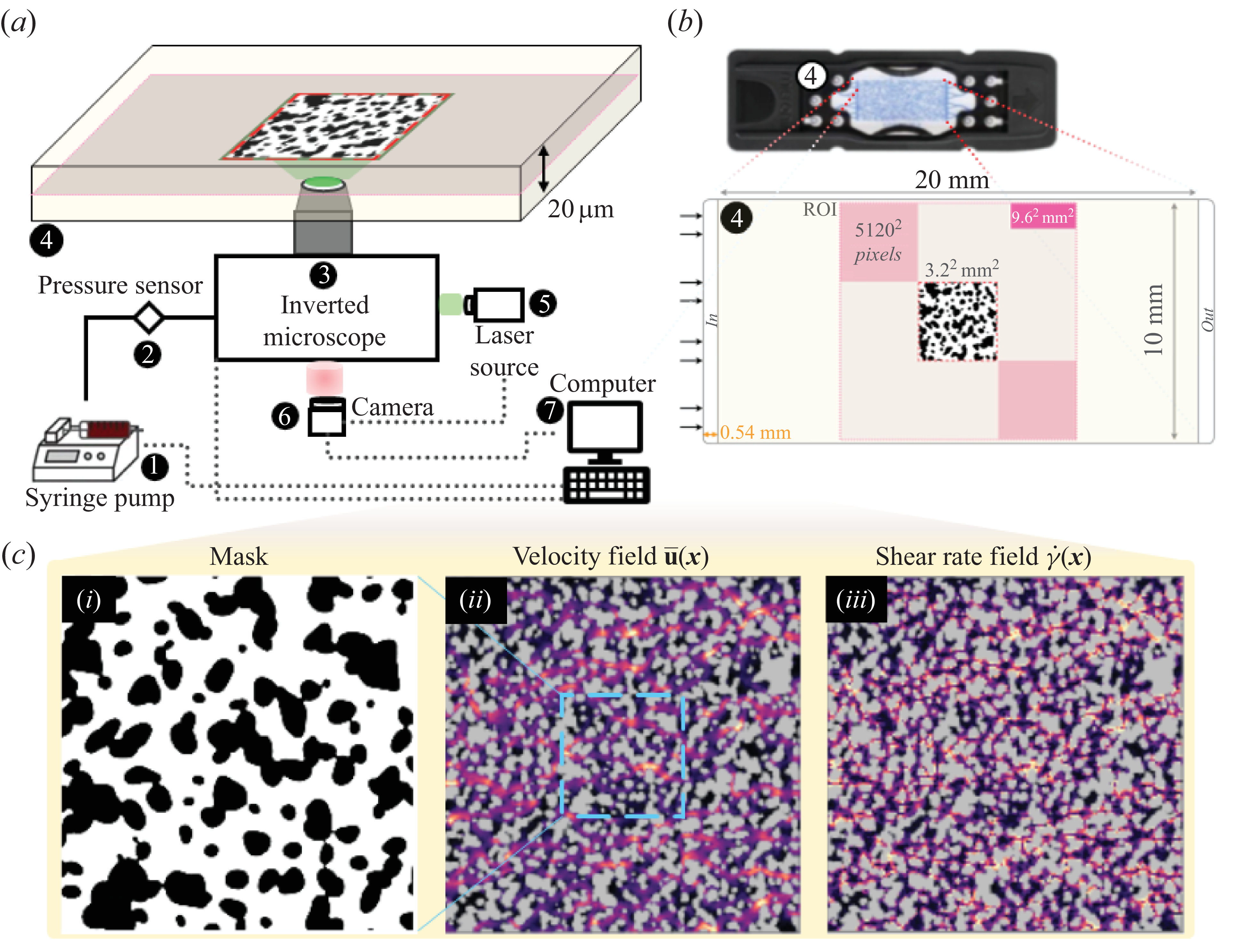


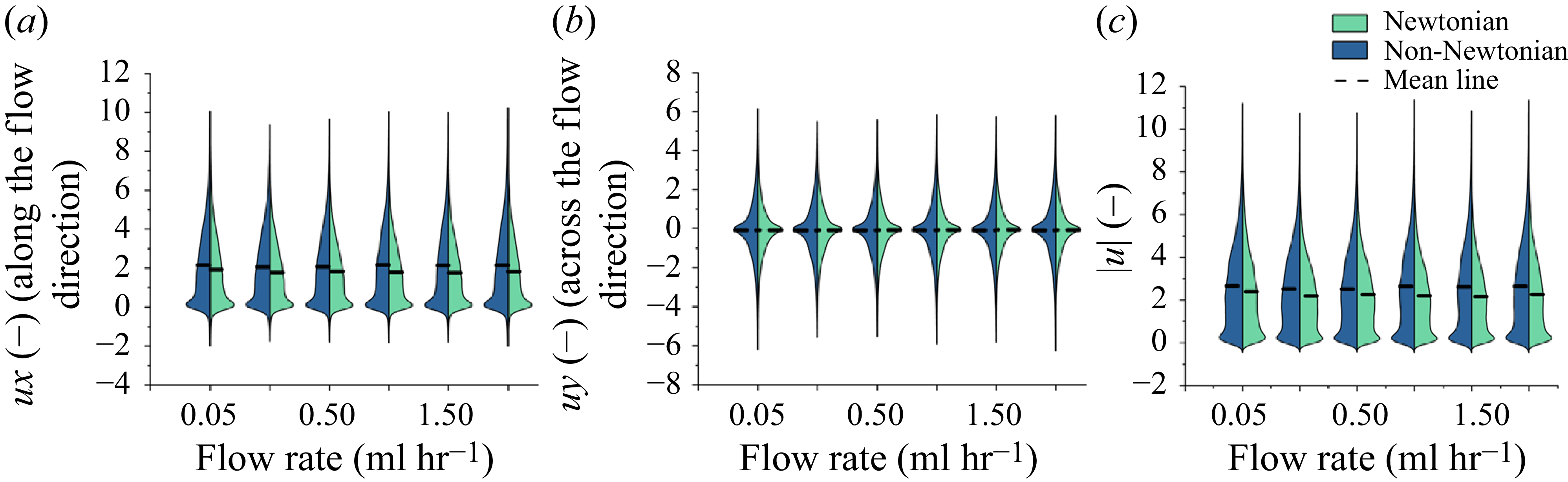


 Open access