





1. Introduction
Neoclassical transport, which is the collisional transport due to toroidicity in tokamaks and stellarators, has been extensively discussed (Hinton & Hazeltine Reference Hinton and Hazeltine1976; Helander & Sigmar Reference Helander and Sigmar2005). One of the main assumptions in these studies is that the gradient length scales of density, temperature and potential are much larger than the ion poloidal gyroradius. Neoclassical theory as described by Hinton & Hazeltine (Reference Hinton and Hazeltine1976) and Helander & Sigmar (Reference Helander and Sigmar2005) is thus limited to regions of weak gradients like the core of a tokamak, where transport is usually dominated by turbulence.
In the pedestal, where gradients are much larger than in the core, ion heat transport has been observed in ASDEX-U (axially symmetric divertor experiment upgrade) to be of the order of neoclassical predictions (Urano et al. Reference Urano, Takizuka, Kamada, Oyama, Takenaga and Miura2005; Viezzer et al. Reference Viezzer2018). Similar observations have been made for internal transport barriers in JET (Joint European Torus) (Tala et al. Reference Tala, Heikkinen, Parail, Baranov and Karttunen2001). Gradient length scales in transport barriers have been measured to be of the order of the ion poloidal gyroradius (Strait et al. Reference Strait1995; McDermott et al. Reference McDermott2009; Viezzer et al. Reference Viezzer2013). Thus, the weak gradient assumption of neoclassical theory breaks down precisely where neoclassical transport becomes important.
Trinczek et al. (Reference Trinczek, Parra, Catto, Calvo and Landreman2023) and Trinczek, Parra & Catto (Reference Trinczek, Parra and Catto2025) extended neoclassical theory into strong gradient regions for the case of a large aspect ratio tokamak with collisionality in the banana regime. This new strong gradient neoclassical theory predicts either enhanced or reduced transport, depending on the profiles of density, temperature and mean parallel flow.
Pedestals as observed in Alcator-C Mod and DIII-D tend to be of sufficiently high collisionality to be close to the banana-plateau transition (Callen et al. Reference Callen, Groebner, Osborne, Canik, Owen., Pankin, Rafiq, Rognlien and Stacey2010; Marr et al. Reference Marr, Lipschultz, Catto, McDermott, Reinke and Simakov2010). To address these higher collisionality pedestals, we present an extension of neoclassical transport in strong gradient regions for the plateau regime that follows the same approach as Trinczek et al. (Reference Trinczek, Parra, Catto, Calvo and Landreman2023) and Trinczek et al. (Reference Trinczek, Parra and Catto2025).
Seol & Shaing (Reference Seol and Shaing2012) aimed to extend neoclassical theory into regions of strong gradients in the plateau regime, but strong mean parallel flow and mean parallel flow gradients were neglected. Pusztai & Catto (Reference Pusztai and Catto2010) and Catto et al. (Reference Catto, Kagan, Landreman and Pusztai2011) had the same objective, but assumed weak temperature gradients as well as weak mean parallel flow and zero neoclassical ion particle flux. Both approaches neglected the poloidal variation in the electric potential that forms in this ordering and has a significant effect on the radial fluxes of energy and particles (Trinczek et al. Reference Trinczek, Parra and Catto2025; Trinczek & Parra Reference Trinczek and Parra2026). We compare our findings with previous work, correct mistakes made in Pusztai & Catto (Reference Pusztai and Catto2010) and Seol & Shaing (Reference Seol and Shaing2012) and conclude that our model is more comprehensive.
In our approach, we keep gradient length scales of the order of the ion poloidal gyroradius for density, potential and temperature. The orbit width of trapped particles is smaller than the gradient scale length by the square root of the inverse aspect ratio. In the limit of small inverse aspect ratio, there is scale separation between the orbit width and the gradient length scale, and a local transport theory can be constructed. We keep the poloidal variation of the electric potential. This poloidal variation modifies transport equations and leads to up–down as well as in–out asymmetry in the plateau regime. The mean parallel flow is allowed to be of the order of the ion thermal velocity. The resulting transport equations explicitly depend on the mean parallel flow. By including sources in the drift kinetic equation, we allow for the possibility of turbulence in the system. Due to these sources, the ion neoclassical particle flux can be much larger than the electron neoclassical particle flux. We derive transport relations for ions and electrons and a formula for the bootstrap current that are modified by strong gradient effects. We also use example profiles to study the modified transport relations and demonstrate that strong gradient effects can enhance or decrease neoclassical transport depending on the input profiles. This is in disagreement with Seol & Shaing (Reference Seol and Shaing2012) who claim that strong gradient effects only ever decrease the neoclassical ion energy flux in the plateau regime in comparison to weak gradient theory.
We start in § 2 with a derivation of neoclassical transport relations for ions and electrons as well as the bootstrap current for collisionality in the boundary between the plateau and the banana regime. We take the collisionality limit for the plateau regime in § 3. We choose a set of example profiles for densities and temperatures of ions and electrons and solve the transport equations assuming either force balance or neoclassical ambipolarity to determine the radial electric field in § 4. We summarise our results in § 5.
2. General equations
We are interested in generalising neoclassical transport theory to allow for gradients of order $L_{n,T,\varPhi }\sim \rho _p$
, where the gradient length scales are defined as
$L_{n,T,\varPhi }\sim \rho _p$
, where the gradient length scales are defined as $L_Q\equiv$ $|\partial \ln Q/\partial r|^{-1}$
,
$|\partial \ln Q/\partial r|^{-1}$
, $n$
is the density,
$n$
is the density, $T$
the ion temperature,
$T$
the ion temperature, $\varPhi$
the electric potential,
$\varPhi$
the electric potential, $r$
is the minor radius and
$r$
is the minor radius and $\rho _p$
is the ion poloidal gyroradius.
$\rho _p$
is the ion poloidal gyroradius.
We start by deriving equations for the distribution function in the freely passing and trapped–barely passing region before we take moments of the drift kinetic equation to find particle, momentum and energy transport of ions and electrons. Throughout this section, we assume that
 \begin{align} \epsilon \ll 1, &\qquad \qquad \nu _\ast \equiv \frac {qR\nu }{\epsilon ^{3/2}v_{t}} \sim 1 \end{align}
and take the subsidiary limit $\epsilon ^{-3/2}\gg \nu _\ast \gg 1$
for the plateau regime in § 3. Here,
$\epsilon ^{-3/2}\gg \nu _\ast \gg 1$
for the plateau regime in § 3. Here, $q$
is the safety factor,
$q$
is the safety factor, $R$
is the major radius,
$R$
is the major radius, $\nu$
is the ion–ion collision frequency,
$\nu$
is the ion–ion collision frequency, $\epsilon \equiv r/R$
is the inverse aspect ratio and
$\epsilon \equiv r/R$
is the inverse aspect ratio and $v_{t}\equiv \sqrt {2T/m}$
is the ion thermal speed with ion mass
$v_{t}\equiv \sqrt {2T/m}$
is the ion thermal speed with ion mass $m$
.
$m$
.
We work in the limit of small inverse aspect ratio $\epsilon \ll 1$
. This implies that the gradient length scales, which we assume to be of the order of the ion poloidal gyroradius,
$\epsilon \ll 1$
. This implies that the gradient length scales, which we assume to be of the order of the ion poloidal gyroradius, $L_{n,T,\varPhi }\sim \rho _p$
, are still much larger than the ion Larmor radius
$L_{n,T,\varPhi }\sim \rho _p$
, are still much larger than the ion Larmor radius $\rho \ll \rho _p\sim q\rho /\epsilon$
. In choosing this ordering, we expand first in
$\rho \ll \rho _p\sim q\rho /\epsilon$
. In choosing this ordering, we expand first in $\epsilon$
and then treat the expansion in collisionality as a subsidiary expansion. Expanding in
$\epsilon$
and then treat the expansion in collisionality as a subsidiary expansion. Expanding in $\epsilon$
first is a viable approach because
$\epsilon$
first is a viable approach because $\rho _\ast \equiv \rho /L_{n,T,\varPhi }\sim \epsilon$
and, thus, we can use the drift kinetic equation, given by
$\rho _\ast \equiv \rho /L_{n,T,\varPhi }\sim \epsilon$
and, thus, we can use the drift kinetic equation, given by
 \begin{align} \big ( v_\parallel \boldsymbol{\hat {b}}+\boldsymbol{v}_E\big )\ \boldsymbol{\cdot }\ &\boldsymbol{\nabla }\theta \frac {\partial f}{\partial \theta }+\left (\boldsymbol{v}_E+\boldsymbol{v}_M\right )\boldsymbol{\cdot }\boldsymbol{\nabla }\psi \frac {\partial f}{\partial \psi }\nonumber \\ &+\left [ \boldsymbol{\hat {b}}+\frac {v_\parallel }{\varOmega }\boldsymbol{\hat {b}}\times \big (\boldsymbol{\hat {b}} \boldsymbol{\cdot } \boldsymbol{\nabla }\boldsymbol{\hat {b}}\big )\right ]\boldsymbol{\cdot }\left (\!-\mu \boldsymbol{\nabla }B+\frac {Ze}{m}\boldsymbol{E}\right )\frac {\partial f}{\partial v_\parallel }=C[f,f]+\varSigma . \end{align}
Here, $\boldsymbol{v}_E=c\boldsymbol{E}\times \boldsymbol{B}/B^2$
is the
$\boldsymbol{v}_E=c\boldsymbol{E}\times \boldsymbol{B}/B^2$
is the $\boldsymbol{E}\times \boldsymbol{B}$
drift,
$\boldsymbol{E}\times \boldsymbol{B}$
drift, $\boldsymbol{v}_M=\mu \boldsymbol{\hat {b}}\times \boldsymbol{\nabla }B/\varOmega +v_\parallel ^2 \boldsymbol{\hat {b}}\times (\boldsymbol{\hat {b}}\boldsymbol{\cdot }\boldsymbol{\nabla }\boldsymbol{\hat {b}})/\varOmega$
is the magnetic drift,
$\boldsymbol{v}_M=\mu \boldsymbol{\hat {b}}\times \boldsymbol{\nabla }B/\varOmega +v_\parallel ^2 \boldsymbol{\hat {b}}\times (\boldsymbol{\hat {b}}\boldsymbol{\cdot }\boldsymbol{\nabla }\boldsymbol{\hat {b}})/\varOmega$
is the magnetic drift, $C[f,f]$
is the Fokker–Planck ion–ion collision operator and
$C[f,f]$
is the Fokker–Planck ion–ion collision operator and $\varSigma \sim \epsilon ^2 v_{t} f/(qR)$
is a source. The electric field
$\varSigma \sim \epsilon ^2 v_{t} f/(qR)$
is a source. The electric field $\boldsymbol{E}=-\boldsymbol{\nabla }\varPhi$
is electrostatic and the electric potential can be split up into
$\boldsymbol{E}=-\boldsymbol{\nabla }\varPhi$
is electrostatic and the electric potential can be split up into $\varPhi (\psi ,\theta )=\phi (\psi )+\phi _\theta (\psi ,\theta )$
, where the poloidally varying piece of the electric potential is small,
$\varPhi (\psi ,\theta )=\phi (\psi )+\phi _\theta (\psi ,\theta )$
, where the poloidally varying piece of the electric potential is small, $\phi _\theta /\phi \sim \epsilon$
. The poloidal angle is
$\phi _\theta /\phi \sim \epsilon$
. The poloidal angle is $\theta$
and
$\theta$
and $\psi$
is the poloidal flux divided by
$\psi$
is the poloidal flux divided by $2\pi$
. The magnetic field is
$2\pi$
. The magnetic field is $\boldsymbol{B}$
, its strength is
$\boldsymbol{B}$
, its strength is $B$
and its direction
$B$
and its direction $\boldsymbol{\hat {b}}\equiv \boldsymbol{B}/B$
,
$\boldsymbol{\hat {b}}\equiv \boldsymbol{B}/B$
, $c$
is the speed of light,
$c$
is the speed of light, $\mu =v_\perp ^2/2B$
is the magnetic moment per unit mass,
$\mu =v_\perp ^2/2B$
is the magnetic moment per unit mass, $v_\perp$
is the perpendicular velocity,
$v_\perp$
is the perpendicular velocity, $v_\parallel$
is the parallel velocity,
$v_\parallel$
is the parallel velocity, $\varOmega =ZeB/(mc)$
is the Larmor frequency and
$\varOmega =ZeB/(mc)$
is the Larmor frequency and $Ze$
is the ion charge. The independent velocity space variables in (2.2) are
$Ze$
is the ion charge. The independent velocity space variables in (2.2) are $v_\parallel$
and
$v_\parallel$
and $\mu$
.
$\mu$
.
For $L_{n,T,\varPhi }\sim \rho _p$
and
$L_{n,T,\varPhi }\sim \rho _p$
and $\epsilon \ll 1$
, the lowest order distribution function is Maxwellian, as derived by Trinczek et al. (Reference Trinczek, Parra, Catto, Calvo and Landreman2023) in their equation (4.9). The distribution function
$\epsilon \ll 1$
, the lowest order distribution function is Maxwellian, as derived by Trinczek et al. (Reference Trinczek, Parra, Catto, Calvo and Landreman2023) in their equation (4.9). The distribution function $f$
can be written as
$f$
can be written as
 \begin{equation} f=f_M+g, \end{equation}
where
 \begin{equation} f_M(v_\parallel ,\mu ,\psi )=n(\psi )\left (\frac {m}{2\pi T(\psi )}\right )^{3/2}\exp \bigg \lbrace {-}\frac {m[v_\parallel -V_\parallel (\psi )]^2}{2T(\psi )}-\frac {m\mu B}{T(\psi )}\bigg \rbrace . \end{equation}
The mean parallel flow $V_\parallel \sim v_{t}$
is included in the Maxwellian to lowest order and can be of the order of the ion thermal velocity. The piece
$V_\parallel \sim v_{t}$
is included in the Maxwellian to lowest order and can be of the order of the ion thermal velocity. The piece $g$
will be shown to be small in
$g$
will be shown to be small in $\sqrt {\epsilon }$
. For a tokamak with concentric circular flux surfaces, we can simplify the drift kinetic equation to lowest order in
$\sqrt {\epsilon }$
. For a tokamak with concentric circular flux surfaces, we can simplify the drift kinetic equation to lowest order in $\epsilon \sim \rho _\ast \ll 1$
and
$\epsilon \sim \rho _\ast \ll 1$
and $\rho _p/R\ll 1$
by using
$\rho _p/R\ll 1$
by using
 \begin{equation} \big ( v_\parallel \boldsymbol{\hat {b}}+\boldsymbol{v}_E\big )\boldsymbol{\cdot }\boldsymbol{\nabla }\theta \simeq \frac {v_\parallel +u}{qR}, \end{equation}
 \begin{equation} \left (\boldsymbol{v}_E+\boldsymbol{v}_M\right )\boldsymbol{\cdot }\boldsymbol{\nabla }\psi \simeq -\frac {I}{\varOmega }\frac {v_\parallel ^2+\mu B}{q R}\frac {r}{R}\sin \theta -\frac {Ic}{qRB}\frac {\partial \phi _\theta }{\partial \theta } \end{equation}
and
 \begin{align} \left [ \boldsymbol{\hat {b}}+\frac {v_\parallel }{\varOmega }\boldsymbol{\hat {b}}\times (\boldsymbol{\hat {b}}\boldsymbol{\cdot }\boldsymbol{\nabla }\boldsymbol{\hat {b}})\right ]\boldsymbol{\cdot }\left (\!-\mu \boldsymbol{\nabla }B+\frac {Ze}{m}\boldsymbol{E}\right )\simeq \frac {v_\parallel u-\mu B}{qR}\frac {r}{R}\sin \theta -\frac {Ze}{qRm}\frac {\partial \phi _\theta }{\partial \theta }. \end{align}
Here, $I\equiv RB_\zeta$
,
$I\equiv RB_\zeta$
, $B_\zeta$
is the toroidal component of the magnetic field, and we used the fact that
$B_\zeta$
is the toroidal component of the magnetic field, and we used the fact that $B\simeq B_0[1-(r/R)\cos \theta ]$
for concentric circular flux surfaces, where
$B\simeq B_0[1-(r/R)\cos \theta ]$
for concentric circular flux surfaces, where $B_0$
is the magnetic field strength on the magnetic axis. We also introduced the velocity
$B_0$
is the magnetic field strength on the magnetic axis. We also introduced the velocity
 \begin{equation} u(\psi ,\theta )\equiv \frac {cI}{B}\frac {\partial \varPhi }{\partial \psi }=\frac {cI}{B}\frac {\partial \phi (\psi )}{\partial \psi }+\frac {cI}{B}\frac {\partial \phi _\theta (\psi ,\theta )}{\partial \psi }, \end{equation}
where $u\sim v_{t}$
. This is the parallel speed of the trapped particles and it is connected to the poloidal projection of the
$u\sim v_{t}$
. This is the parallel speed of the trapped particles and it is connected to the poloidal projection of the $E\times B$
drift. Note that this definition is slightly different from that by Trinczek et al. (Reference Trinczek, Parra, Catto, Calvo and Landreman2023, Equation (3.9)), where
$E\times B$
drift. Note that this definition is slightly different from that by Trinczek et al. (Reference Trinczek, Parra, Catto, Calvo and Landreman2023, Equation (3.9)), where $u$
was defined to be proportional to the derivative of only the poloidally independent part of the electric potential. The difference between the two definitions will turn out to be negligible for most of our discussion. With these results and recalling that
$u$
was defined to be proportional to the derivative of only the poloidally independent part of the electric potential. The difference between the two definitions will turn out to be negligible for most of our discussion. With these results and recalling that $\rho _\ast \sim \epsilon \ll 1$
and
$\rho _\ast \sim \epsilon \ll 1$
and $\nu _\ast \sim 1$
, the drift kinetic equation (2.2) for ions becomes
$\nu _\ast \sim 1$
, the drift kinetic equation (2.2) for ions becomes
 \begin{align} &\frac {v_\parallel +u}{qR}\frac {\partial g}{\partial \theta }+\left (\frac {v_\parallel u-\mu B}{qR}\frac {r}{R}\sin \theta -\frac {Ze}{qRm}\frac {\partial \phi _\theta }{\partial \theta }\right )\frac {\partial g}{\partial v_\parallel } \nonumber\\[4pt]& \!\!\quad -\frac {I}{\varOmega } \left (\frac {v_\parallel ^2+\mu B}{q R}\frac {r}{R}\sin \theta +\frac {Ze}{qRm}\frac {\partial \phi _\theta }{\partial \theta }\right )\frac {\partial g}{\partial \psi } =\frac {I}{\varOmega }\left (\frac {v_\parallel ^2+\mu B}{q R}\frac {r}{R}\sin \theta +\frac {Ze}{qRm}\frac {\partial \phi _\theta }{\partial \theta }\right )\nonumber\\[4pt]& \!\!\quad \times \Bigg [\!\frac {\partial }{\partial \psi }\ln p + \left (\frac {m(v_\parallel -V_\parallel )^2}{2T}+\frac {m\mu B}{T}-\frac {5}{2}\right )\!\frac {\partial }{\partial \psi }\ln T + \frac {m(v_\parallel -V_\parallel )}{T}\!\left (\frac {\partial V_\parallel }{\partial \psi }-\frac {\varOmega }{I}\right )\!\!\Bigg ]f_M\nonumber\\[4pt]& \!\!\quad +\frac {v_\parallel +u}{qR}\frac {r}{R}\sin \theta \frac {m}{T}[v_\parallel (v_\parallel -V_\parallel )+\mu B]f_M+C^{(l)}[g]+\varSigma , \end{align}
with the ion pressure $p=nT$
. The linearised collision operator for ions was introduced by Trinczek et al. (Reference Trinczek, Parra, Catto, Calvo and Landreman2023) in their equation (4.18) as
$p=nT$
. The linearised collision operator for ions was introduced by Trinczek et al. (Reference Trinczek, Parra, Catto, Calvo and Landreman2023) in their equation (4.18) as
 \begin{align} C^{(l)}[g] & = \lambda \boldsymbol{\nabla} _v\boldsymbol{\cdot }\left [\int \text{d}^3v'f_M f'_M \boldsymbol{\nabla} _\omega \boldsymbol{\nabla} _\omega \omega \boldsymbol{\cdot }\left (\boldsymbol{\nabla} _v\left (\frac {g}{f_M}\right )-\boldsymbol{\nabla} _{v'}\left (\frac {g'}{f_M'}\right )\right )\right ]\nonumber\\[3pt]& \simeq \boldsymbol{\nabla} _v\boldsymbol{\cdot }\bigg [f_M {\unicode{x1D648}} \boldsymbol{\cdot }\boldsymbol{\nabla} _v\left (\frac {g}{f_M}\right )-\lambda f_M\int \mathrm{d}^3v' f'_M \boldsymbol{\nabla} _\omega \boldsymbol{\nabla} _\omega \omega \boldsymbol{\cdot }\boldsymbol{\nabla} _{v'}\left (\frac {g'}{f'_M}\right )\bigg]\nonumber\\[3pt]& \equiv \boldsymbol{\nabla} _v\boldsymbol{\cdot }\boldsymbol{M}_{\text{col}}, \end{align}
where primed quantities denote functions of primed velocities, $\lambda =2\pi Z^4e^4 \log \varLambda /m^2$
,
$\lambda =2\pi Z^4e^4 \log \varLambda /m^2$
, $\boldsymbol{\omega }=\boldsymbol{v}-\boldsymbol{v}'$
,
$\boldsymbol{\omega }=\boldsymbol{v}-\boldsymbol{v}'$
, $\omega =|\boldsymbol{\omega }|$
and
$\omega =|\boldsymbol{\omega }|$
and $\log \varLambda$
is the Coulomb logarithm. We introduce the matrix
$\log \varLambda$
is the Coulomb logarithm. We introduce the matrix
 \begin{align} &\qquad {\unicode{x1D648}}=\frac {\nu _\perp }{4}\big [|\boldsymbol{v}-V_\parallel \boldsymbol{\hat {b}}|^2{\unicode{x1D644}}-(\boldsymbol{v}-V_\parallel \boldsymbol{\hat {b}})(\boldsymbol{v}-V_\parallel \boldsymbol{\hat {b}})\big]+\frac {\nu _\parallel }{2}(\boldsymbol{v}-V_\parallel \boldsymbol{\hat {b}})(\boldsymbol{v}-V_\parallel \boldsymbol{\hat {b}}), \\[-8pt]\nonumber \end{align}
 \begin{align} &\nu _\perp =3\sqrt {\frac {\pi }{2}}\nu \frac {\varXi (x)-\varPsi (x)}{x^3}, \quad \nu _\parallel =3\sqrt {\frac {\pi }{2}}\nu \frac {\varPsi (x)}{x^3} \quad \text{and} \quad \nu = \frac {4\sqrt {\pi } Z^4e^4n\log \varLambda }{3T^{3/2}m^{1/2}}, \end{align}
where $x=\sqrt {m/(2T)}|\boldsymbol{v}-V_\parallel \boldsymbol{\hat {b}}|$
,
$x=\sqrt {m/(2T)}|\boldsymbol{v}-V_\parallel \boldsymbol{\hat {b}}|$
, $\varXi (x)=\text{erf}(x)$
and
$\varXi (x)=\text{erf}(x)$
and $\varPsi (x)=(\varXi - x\varXi ')/(2x^2)$
is the Chandrasekhar function. The collision operator expressed in the independent velocity space variables
$\varPsi (x)=(\varXi - x\varXi ')/(2x^2)$
is the Chandrasekhar function. The collision operator expressed in the independent velocity space variables $v_\parallel$
and
$v_\parallel$
and $\mu$
can be written as
$\mu$
can be written as
 \begin{equation} C^{(l)}[g]= \frac {\partial }{\partial v_\parallel } (\boldsymbol{\hat b}\boldsymbol{\cdot }\boldsymbol{M}_{\text{col}})+\frac {\partial }{\partial \mu }\left ( \frac {\boldsymbol{v}_\perp }{B}\boldsymbol{\cdot }\boldsymbol{M}_{\text{col}} \right )\!. \end{equation}
For some calculations, it is convenient to write the left-hand side of the drift kinetic equation in (2.9) in a conservative form:
 \begin{align} &\frac {\partial }{\partial \theta }\left (\frac {v_\parallel +u}{qR}g\right )+\frac {\partial }{\partial v_\parallel }\left [\left (\frac {v_\parallel u-\mu B}{qR}\frac {r}{R}\sin \theta -\frac {Ze}{qRm}\frac {\partial \phi _\theta }{\partial \theta }\right )g\right ] \nonumber\\[4pt]& \quad -\frac {\partial }{\partial \psi }\left [\frac {I}{\varOmega }\left (\frac {v_\parallel ^2+\mu B}{q R}\frac {r}{R}\sin \theta +\frac {Ze}{qRm}\frac {\partial \phi _\theta }{\partial \theta }\right )g\right ] =\frac {I}{\varOmega }\left (\frac {v_\parallel ^2+\mu B}{q R}\frac {r}{R}\sin \theta +\frac {Ze}{qRm}\frac {\partial \phi _\theta }{\partial \theta }\right )\nonumber\\[4pt]& \quad \times \Bigg [\frac {\partial }{\partial \psi }\ln p+\left (\frac {m(v_\parallel -V_\parallel )^2}{2T}+\frac {m\mu B}{T}-\frac {5}{2}\right )\frac {\partial }{\partial \psi }\ln T +\frac {m(v_\parallel -V_\parallel )}{T}\left (\frac {\partial V_\parallel }{\partial \psi }-\frac {\varOmega }{I}\right )\Bigg ]f_M\nonumber\\[4pt]& \quad +\frac {v_\parallel +u}{qR}\frac {r}{R}\sin \theta \frac {m}{T}[v_\parallel (v_\parallel -V_\parallel )+\mu B]f_M+C^{(l)}[g]+\varSigma . \end{align}
Note that to obtain this expression, we have used $\partial u/\partial \theta \simeq -u(r/R)\sin \theta +(cI/B)(\partial ^2\phi _\theta /\partial \psi \partial \theta )$
. For this relation to hold, we needed to keep
$\partial u/\partial \theta \simeq -u(r/R)\sin \theta +(cI/B)(\partial ^2\phi _\theta /\partial \psi \partial \theta )$
. For this relation to hold, we needed to keep $\phi _\theta$
in the definition of
$\phi _\theta$
in the definition of $u$
in (2.8).
$u$
in (2.8).
As discussed in detail in Trinczek et al. (Reference Trinczek, Parra, Catto, Calvo and Landreman2023), Trinczek et al. (Reference Trinczek, Parra and Catto2025) and Trinczek & Parra (Reference Trinczek and Parra2026), trapped particles are particles with velocity $v_\parallel \simeq -u$
. See, for example, the discussion below equation (3.10) in Trinczek et al. (Reference Trinczek, Parra, Catto, Calvo and Landreman2023). For this reason, it is useful to make a change of variables from
$v_\parallel \simeq -u$
. See, for example, the discussion below equation (3.10) in Trinczek et al. (Reference Trinczek, Parra, Catto, Calvo and Landreman2023). For this reason, it is useful to make a change of variables from $v_\parallel$
to
$v_\parallel$
to $w\equiv v_\parallel +u$
in the trapped–barely passing region:
$w\equiv v_\parallel +u$
in the trapped–barely passing region:
 \begin{equation} \frac {\partial g}{\partial \psi }\Bigg \vert _{\theta ,v_\parallel }=\frac {\partial g}{\partial \psi }\Bigg \vert _{\theta ,w}+\frac {\partial u}{\partial \psi }\Bigg \vert _{\theta }\frac {\partial g}{\partial w}\Bigg \rvert _{\theta ,\psi }, \end{equation}
 \begin{equation} \frac {\partial g}{\partial v_\parallel }\Bigg \rvert _{\theta ,\psi }=\frac {\partial g}{\partial w}\Bigg \rvert _{\theta ,\psi }, \end{equation}
 \begin{equation} \frac {\partial g}{\partial \theta }\Bigg \rvert _{v_\parallel ,\psi }=\frac {\partial g}{\partial \theta }\Bigg \rvert _{w,\psi }+\frac {\partial u}{\partial \theta }\Bigg \rvert _{\psi }\frac {\partial g}{\partial w}\Bigg \rvert _{\theta ,\psi }. \end{equation}
The change of variables from $v_\parallel$
to
$v_\parallel$
to $w$
is convenient to distinguish the trapped–barely passing and the freely passing regions. In the freely passing region,
$w$
is convenient to distinguish the trapped–barely passing and the freely passing regions. In the freely passing region, $w\sim v_{t}$
and, hence, we assume that
$w\sim v_{t}$
and, hence, we assume that $\partial g^p/\partial w\sim g^p/v_{t}$
, whereas in the trapped–barely passing region
$\partial g^p/\partial w\sim g^p/v_{t}$
, whereas in the trapped–barely passing region $w\sim \epsilon ^{1/2} v_{t}$
and, thus,
$w\sim \epsilon ^{1/2} v_{t}$
and, thus, $\partial g^{t,bp}/\partial w \sim g^{t,bp}/(\epsilon ^{1/2} v_{t})$
. Here,
$\partial g^{t,bp}/\partial w \sim g^{t,bp}/(\epsilon ^{1/2} v_{t})$
. Here, $g^p$
denotes the distribution function of freely passing particles and
$g^p$
denotes the distribution function of freely passing particles and $g^{t,bp}$
is the distribution function in the trapped and barely passing region. Note that the second term in (2.17) is small in
$g^{t,bp}$
is the distribution function in the trapped and barely passing region. Note that the second term in (2.17) is small in $\epsilon$
because
$\epsilon$
because $u$
depends on
$u$
depends on $\theta$
through the derivatives of
$\theta$
through the derivatives of $\phi _\theta$
and
$\phi _\theta$
and $B$
, as can be seen from (2.8). In the trapped–barely passing region, we use the conservative form of the drift kinetic equation in the variables
$B$
, as can be seen from (2.8). In the trapped–barely passing region, we use the conservative form of the drift kinetic equation in the variables $(\psi ,\theta , w,\mu )$
:
$(\psi ,\theta , w,\mu )$
:
 \begin{align} &\frac {\partial }{\partial \theta }\left (\frac {w}{qR}g\right )+\frac {\partial }{\partial w}\left (\frac {\partial u}{\partial \theta }\frac {1}{qR}w g\right ) -\frac {\partial }{\partial \psi }\left [\frac {I}{\varOmega }\left (\frac {(w-u)^2+\mu B}{q R}\frac {r}{R}\sin \theta +\frac {Ze}{qRm}\frac {\partial \phi _\theta }{\partial \theta }\right )g\right ]\nonumber \\[2pt] &\quad +\frac {\partial }{\partial w}\left [S\left (\frac {(w-u) u-\mu B}{qR}\frac {r}{R}\sin \theta -\frac {Ze}{qRm}\frac {\partial \phi _\theta }{\partial \theta }\right )g-\frac {I}{\varOmega }\frac {\partial u}{\partial \psi }\frac {(w-u) w}{qR}\frac {r}{R}\sin \theta g\right ]\nonumber \\[2pt] &\quad -\frac {I}{\varOmega }\left (\frac {(w-u)^2+\mu B}{q R}\frac {r}{R}\sin \theta +\frac {Ze}{qRm}\frac {\partial \phi _\theta }{\partial \theta }\right )\Bigg [\frac {\partial }{\partial \psi }\ln p+\frac {m(w-u-V_\parallel )}{T}\left (\frac {\partial V_\parallel }{\partial \psi }-\frac {\varOmega }{I}\right )\nonumber \\[2pt] &\quad +\left (\frac {m(w-u-V_\parallel )^2}{2T}+\frac {m\mu B}{T}-\frac {5}{2}\right )\frac {\partial }{\partial \psi }\ln T \Bigg ]f_M\nonumber \\[2pt] &\quad -\frac {w}{qR}\frac {r}{R}\sin \theta \frac {m}{T}[(w-u)(w-u-V_\parallel )+\mu B]f_M=C^{(l)}[g]+\varSigma . \end{align}
Here, we introduced the squeezing factor $S$
as
$S$
as
 \begin{equation} S\equiv 1+\frac {cI^2}{B\varOmega }\frac {{\partial ^2}{\varPhi }}{\partial {\psi }^{2}}. \end{equation}
Going forward, when convenient, we will abbreviate the drift kinetic operator applied on $g$
and
$g$
and $f_M$
as
$f_M$
as $\mathcal{L}$
, allowing us to rewrite (2.9), (2.14) and (2.18) as
$\mathcal{L}$
, allowing us to rewrite (2.9), (2.14) and (2.18) as
 \begin{equation} \mathcal{L}[g]+\mathcal{L}[f_M]=C^{(l)}[g]+\varSigma . \end{equation}
2.1. Distribution function
Velocity space can be separated into the trapped–barely passing region and the freely passing region. We denote the distribution function in the freely passing region as $g^p$
and in the trapped–barely passing region as
$g^p$
and in the trapped–barely passing region as $g^{t,bp}$
. It will be shown later that the distribution functions in these two regions are governed by different equations. The integration over the respective regions is defined as
$g^{t,bp}$
. It will be shown later that the distribution functions in these two regions are governed by different equations. The integration over the respective regions is defined as
 \begin{equation} \int _{V_{tbp}}\mathrm{d}^3v\: \equiv \lim _{W\rightarrow \infty }\int _0^\infty \mathrm{d}\mu \: \int _{-W}^W\mathrm{d}w\:2\pi B \end{equation}
in the trapped–barely passing region and
 \begin{equation} \int _{V_{p}}\mathrm{d}^3v\: \equiv \lim _{\delta \rightarrow 0}\int _0^\infty \mathrm{d}\mu \: \int _{-\infty }^{-u-\delta }\mathrm{d}v_\parallel \: 2\pi B+\lim _{\delta \rightarrow 0}\int _0^\infty \mathrm{d}\mu \: \int _{-u+\delta }^{\infty }\mathrm{d}v_\parallel \: 2\pi B, \end{equation}
where $\delta \gt 0$
, in the freely passing region.
$\delta \gt 0$
, in the freely passing region.
The distribution functions have to match asymptotically, i.e.
 \begin{equation} g^p(v_\parallel \rightarrow -u^+)=g^{t,bp}(w\rightarrow \infty )\quad \text{and}\quad g^p(v_\parallel \rightarrow -u^-)=g^{t,bp}(w\rightarrow -\infty ). \end{equation}
Here, $-u^+$
(
$-u^+$
( $-u^-$
) indicates that
$-u^-$
) indicates that $-u$
is approached from the positive (negative) side. The distribution function
$-u$
is approached from the positive (negative) side. The distribution function $g^p$
is discontinuous across the trapped–barely passing region. This jump
$g^p$
is discontinuous across the trapped–barely passing region. This jump $\Delta g^p$
matches the jump in the trapped–barely passing distribution function
$\Delta g^p$
matches the jump in the trapped–barely passing distribution function
 \begin{equation} \Delta g^p\equiv g^p(v_\parallel \rightarrow -u^+)-g^p(v_\parallel \rightarrow -u^-)=g^{t,bp}(w\rightarrow \infty )-g^{t,bp}(w\rightarrow -\infty ). \end{equation}
With these definitions, we can also introduce the linearised collision operator in the freely passing region
 \begin{align} C_p^{(l)}[g]= \boldsymbol{\nabla} _v\boldsymbol{\cdot }\Bigg [f_M {\unicode{x1D648}} \boldsymbol{\cdot }\boldsymbol{\nabla} _v\left (\frac {g^p}{f_M}\right )-\lambda f_M\int _{V_{tbp}}\mathrm{d}^3v' f'_M \boldsymbol{\nabla} _\omega \boldsymbol{\nabla} _\omega \omega \boldsymbol{\cdot }\boldsymbol{\nabla} _v'\left (\frac {g^{t,bp'}}{f'_M}\right )\nonumber \\ -\lambda f_M\int _{V_{p}}\mathrm{d}^3v' f'_M \boldsymbol{\nabla} _\omega \boldsymbol{\nabla} _\omega \omega \boldsymbol{\cdot }\boldsymbol{\nabla} _v'\left (\frac {g^{p'}}{f'_M}\right )\Bigg ] \equiv \boldsymbol{\nabla} _v\boldsymbol{\cdot }\boldsymbol{M}_{\text{col}}^p, \end{align}
and the linearised collision operator in the trapped–barely passing region
 \begin{align} C_{t,bp}^{(l)}[g]= \boldsymbol{\nabla} _v\boldsymbol{\cdot }\Bigg [f_M {\unicode{x1D648}} \boldsymbol{\cdot }\boldsymbol{\nabla} _v\left (\frac {g^{t,bp}}{f_M}\right )-\lambda f_M\int _{V_{tbp}}\mathrm{d}^3v' f'_M \boldsymbol{\nabla} _\omega \boldsymbol{\nabla} _\omega \omega \boldsymbol{\cdot }\boldsymbol{\nabla} _v'\left (\frac {g^{t,bp'}}{f'_M}\right )\nonumber \\ -\lambda f_M\int _{V_{p}}\mathrm{d}^3v' f'_M \boldsymbol{\nabla} _\omega \boldsymbol{\nabla} _\omega \omega \boldsymbol{\cdot }\boldsymbol{\nabla} _v'\left (\frac {g^{p'}}{f'_M}\right )\Bigg ] \equiv \boldsymbol{\nabla} _v\boldsymbol{\cdot }\boldsymbol{M}_{\text{col}}^{t,bp}. \end{align}
We expand the distribution function $g$
in the size of the trapped region
$g$
in the size of the trapped region $\epsilon ^{1/2}$
, i.e.
$\epsilon ^{1/2}$
, i.e.
 \begin{align} g=g_0+g_1+\ldots , \end{align}
where $g_1\sim \epsilon ^{1/2}g_0$
and
$g_1\sim \epsilon ^{1/2}g_0$
and $g_0\sim \epsilon ^{1/2}f_M$
. This expansion is valid in both the trapped–barely passing and the freely passing regions.
$g_0\sim \epsilon ^{1/2}f_M$
. This expansion is valid in both the trapped–barely passing and the freely passing regions.
In the freely passing region, $g^p$
is independent of
$g^p$
is independent of $\theta$
to lowest order in
$\theta$
to lowest order in $\sqrt {\epsilon }$
, as shown by Trinczek et al. (Reference Trinczek, Parra, Catto, Calvo and Landreman2023). The
$\sqrt {\epsilon }$
, as shown by Trinczek et al. (Reference Trinczek, Parra, Catto, Calvo and Landreman2023). The $\theta$
-dependent part was calculated by Trinczek et al. (Reference Trinczek, Parra, Catto, Calvo and Landreman2023) in their equation (4.53) and yields
$\theta$
-dependent part was calculated by Trinczek et al. (Reference Trinczek, Parra, Catto, Calvo and Landreman2023) in their equation (4.53) and yields
 \begin{align} & g^p-\langle g^p\rangle _\psi = -\frac {I}{\varOmega }\frac {r}{R}\frac {\big(v_\parallel ^2+\mu B\big) \cos {\theta }-ZeR\phi _\theta /mr}{v_\parallel +u}\Bigg [\frac {\partial }{\partial \psi }\ln {p} +\frac {m(v_\parallel - V_\parallel )}{T}\left (\frac {\partial V_\parallel }{\partial \psi }-\frac {\varOmega }{I}\right )\nonumber\\& \!\!\quad + \left (\frac {m(v_\parallel -V_\parallel )^2}{2T}+\frac {m\mu B}{T}-\frac {5}{2}\right )\frac {\partial }{\partial \psi }\ln {T}\Bigg ]f_M -\frac {r}{R}\cos {\theta }\frac {m}{T}\left [v_\parallel (v_\parallel -V_\parallel )+\mu B \right ]\!f_M\sim \epsilon f_M. \end{align}
Here, we introduced the flux surface average
 \begin{equation} \langle \ldots \rangle _\psi =\int \frac {\mathrm{d}\theta }{2\pi }(\ldots ). \end{equation}
The expression (2.28) can also be found by noting that the terms proportional to $\partial g/\partial v_\parallel$
and
$\partial g/\partial v_\parallel$
and $\partial g/\partial \psi$
in (2.9) are negligible in the freely passing region, where
$\partial g/\partial \psi$
in (2.9) are negligible in the freely passing region, where $\partial /\partial v_\parallel \sim 1/v_t$
. The collision operator is negligible to lowest order for collisionalities
$\partial /\partial v_\parallel \sim 1/v_t$
. The collision operator is negligible to lowest order for collisionalities $\nu _\ast \ll \epsilon ^{-3/2}$
. The
$\nu _\ast \ll \epsilon ^{-3/2}$
. The $\theta$
dependence in the trapped–barely passing region has to match the freely passing solution according to (2.23). Thus, any
$\theta$
dependence in the trapped–barely passing region has to match the freely passing solution according to (2.23). Thus, any $\theta$
dependence in
$\theta$
dependence in $g_0^{t,bp}$
has to decay as
$g_0^{t,bp}$
has to decay as $w\rightarrow \pm \infty$
and cannot contribute to the jump
$w\rightarrow \pm \infty$
and cannot contribute to the jump $\Delta g^p$
.
$\Delta g^p$
.
In the trapped–barely passing region, we can use the fact that $w\simeq 0$
to lowest order. The linearised collision operator (2.26) to lowest order in
$w\simeq 0$
to lowest order. The linearised collision operator (2.26) to lowest order in $\epsilon$
is
$\epsilon$
is
 \begin{equation} C_{t,bp}^{(l)}[g]=\mathsf{M}_\parallel \frac {\partial ^2 {g^{t,bp}_0}}{\partial {w}^{2}}, \end{equation}
where we defined
 \begin{equation} \mathsf{M}_\parallel \equiv \boldsymbol{\hat {b}}\boldsymbol{\cdot }{\unicode{x1D648}}\boldsymbol{\cdot }\boldsymbol{\hat {b}}\Big \rvert _{w=0}= \frac {\nu _\perp }{2}\mu B+\frac {\nu _\parallel }{2}(u+V_\parallel )^2. \end{equation}
Here, $\nu _\perp$
and
$\nu _\perp$
and $\nu _\parallel$
are evaluated at
$\nu _\parallel$
are evaluated at $w=0$
. We find that (2.18) is, to lowest order in
$w=0$
. We find that (2.18) is, to lowest order in $\sqrt {\epsilon }$
and for
$\sqrt {\epsilon }$
and for $\nu _\ast \sim 1$
,
$\nu _\ast \sim 1$
,
 \begin{align} &\frac {\partial }{\partial \theta }\left (\frac {w}{qR}g_0^{t,bp}\right )-S\frac {\partial }{\partial w}\left [\mathcal{P}(\theta )\frac {r}{R}\frac {1}{qR}g_0^{t,bp}\right ]\nonumber \\ &\qquad\qquad\qquad\qquad\qquad\qquad =\frac {I}{\varOmega }\mathcal{P}(\theta )\frac {r}{R}\frac {1}{qR}\mathcal{D}f_M(w=0)+\mathsf{M}_\parallel \frac {\partial ^2{g^{t,bp}_0}}{\partial {w}^2}, \end{align}
where we introduced the poloidal dependence
 \begin{equation} \mathcal{P}(\theta )=(u^2+\mu B)\sin \theta +\frac {ZeR}{mr}\frac {\partial \phi _\theta }{\partial \theta } \end{equation}
and the derivative term
 \begin{equation} \mathcal{D}\equiv \frac {\partial }{\partial \psi }\ln {p} -\frac {m(u+ V_\parallel )}{T}\left (\frac {\partial V_\parallel }{\partial \psi }-\frac {\varOmega }{I}\right ) +\left (\frac {m(u+V_\parallel )^2}{2T}+\frac {m\mu B}{T}-\frac {5}{2}\right )\frac {\partial }{\partial \psi }\ln {T}. \end{equation}
In the large $w$
limit, (2.32) reduces to
$w$
limit, (2.32) reduces to
 \begin{equation} \frac {\partial }{\partial \theta }\left (\frac {w}{qR}g_0^{t,bp}\right ) =\frac {I}{\varOmega }\mathcal{P}(\theta )\frac {r}{R}\frac {1}{qR}\mathcal{D}f_M(w=0). \end{equation}
From this, we find that the $\theta$
-dependent piece of
$\theta$
-dependent piece of $g^{t,bp}_0$
decays as
$g^{t,bp}_0$
decays as $\sim 1/w$
for
$\sim 1/w$
for $w\rightarrow \infty$
as expected. Furthermore, we recover the terms in expression (2.28) that diverge as
$w\rightarrow \infty$
as expected. Furthermore, we recover the terms in expression (2.28) that diverge as $1/w$
for small
$1/w$
for small $w$
. The other terms in (2.28) match the large
$w$
. The other terms in (2.28) match the large $w$
limit of the next-order correction
$w$
limit of the next-order correction $g_1^{t,bp}$
. Equation (2.32) is sufficient to determine neoclassical transport quantities and we will not solve for
$g_1^{t,bp}$
. Equation (2.32) is sufficient to determine neoclassical transport quantities and we will not solve for $g_1^{t,bp}$
in this paper.
$g_1^{t,bp}$
in this paper.
2.2. Moment equations
We are interested in calculating particle, parallel momentum and energy transport in the limit of $\epsilon \ll 1$
and
$\epsilon \ll 1$
and $\nu _\ast \sim 1$
. The transport relations are associated with moments of the drift kinetic equation. The integration has to treat freely passing and trapped–barely passing particles separately. First, we discuss the freely passing region.
$\nu _\ast \sim 1$
. The transport relations are associated with moments of the drift kinetic equation. The integration has to treat freely passing and trapped–barely passing particles separately. First, we discuss the freely passing region.
The transit average of (2.9) appears to have many contributions by terms proportional to $f_M$
and terms proportional to derivatives of
$f_M$
and terms proportional to derivatives of $g$
. However, the
$g$
. However, the $\theta$
dependence of
$\theta$
dependence of $f_M$
and
$f_M$
and $g^p$
is of order O
$g^p$
is of order O $(\epsilon )$
; see (2.28). Thus, the transit average of (2.9) in the freely passing region to lowest order in
$(\epsilon )$
; see (2.28). Thus, the transit average of (2.9) in the freely passing region to lowest order in $\epsilon$
reduces to
$\epsilon$
reduces to
 \begin{equation} \big\langle C_p^{(l)}[g]\big\rangle _\tau \simeq -\langle \varSigma \rangle _\tau . \end{equation}
We define the transit average for passing particles as
 \begin{align} \langle \ldots \rangle _\tau =\frac {1}{\tau } \int _0^{2\pi }\mathrm{d}\theta \:\frac { qR}{v_\parallel +u}(\ldots ), \end{align}
where
 \begin{align} \tau =\int _0^{2\pi }\mathrm{d}\theta \:\frac {qR}{v_\parallel +u}. \end{align}
Trinczek et al. (Reference Trinczek, Parra, Catto, Calvo and Landreman2023) introduced a new set of variables that is based on conserved quantities, which proved (2.36) to be exact if the new variables are held fixed in the transit average; see their equation (4.21). The difference between the new variables and $\lbrace v_\parallel ,\psi \rbrace$
is small in
$\lbrace v_\parallel ,\psi \rbrace$
is small in $\epsilon$
for freely passing particles and negligible for the purpose of this paper. We derive transport equations of particles, momentum and energy by taking moments of the drift kinetic equation (2.36).
$\epsilon$
for freely passing particles and negligible for the purpose of this paper. We derive transport equations of particles, momentum and energy by taking moments of the drift kinetic equation (2.36).
The integration of (2.36) over the freely passing region to find the particle transport is
 \begin{equation} \int _{V_p}\mathrm{d}^3v\: \big\langle C_p^{(l)}[g]\big\rangle _\tau =-\int _{V_p}\mathrm{d}^3v\:\langle \varSigma \rangle _\tau . \end{equation}
The integration over the freely passing region is defined as
 \begin{equation} \int _{V_p}\mathrm{d}^3v\:(\ldots )=\int _{-\infty }^{-u^-}\mathrm{d}v_\parallel \:\int _0^\infty \mathrm{d}\mu \:2\pi B(\ldots )+\int _{-u^+}^{\infty }\mathrm{d}v_\parallel \:\int _0^\infty \mathrm{d}\mu \:2\pi B(\ldots ), \end{equation}
where the limits $-u^-$
and
$-u^-$
and $-u^+$
indicate that
$-u^+$
indicate that $g^p$
is not continuous at
$g^p$
is not continuous at $-u$
and we need to distinguish between the two sides of
$-u$
and we need to distinguish between the two sides of $-u$
.
$-u$
.
Because the change in parallel velocity along the orbit is small for freely passing particles, it is possible to replace transit averages by flux surface averages, $\langle \ldots \rangle _\tau \simeq \langle \ldots \rangle _\psi$
. The integration over
$\langle \ldots \rangle _\tau \simeq \langle \ldots \rangle _\psi$
. The integration over $\mu$
in (2.39) cancels out the
$\mu$
in (2.39) cancels out the $\mu$
derivative in the divergence of the collision operator in (2.13) and (2.39) becomes
$\mu$
derivative in the divergence of the collision operator in (2.13) and (2.39) becomes
 \begin{equation} \bigg \langle\! \int _{V_p}\mathrm{d}^3v\:\frac {\partial }{\partial v_\parallel }\big( \boldsymbol{\hat {b}}\boldsymbol{\cdot }\boldsymbol{M}_{\text{col}}^p\big)\bigg \rangle _\psi \simeq -\bigg \langle\! \int _{V_p} \mathrm{d}^3 v\:\varSigma \bigg \rangle _\psi . \end{equation}
The integration over $v_\parallel$
gives a jump contribution,
$v_\parallel$
gives a jump contribution,
 \begin{equation} \bigg \langle\! \int \mathrm{d}\mu \:2\pi B\Delta \big[\boldsymbol{\hat {b}}\boldsymbol{\cdot }\boldsymbol{M}_{\text{col}}^p \big] \bigg \rangle _\psi \simeq \bigg \langle\! \int _{V_p} \mathrm{d}^3 v\:\varSigma \bigg \rangle _\psi . \end{equation}
In the freely passing region, the jump of a function $\Delta \mathcal{F}^p$
across the trapped–barely passing region is defined as
$\Delta \mathcal{F}^p$
across the trapped–barely passing region is defined as
 \begin{equation} \Delta \mathcal{F}^p\equiv \mathcal{F}^p(v_\parallel \rightarrow -u^+)-\mathcal{F}^p(v_\parallel \rightarrow -u^-). \end{equation}
By integrating the drift kinetic equation over the freely passing region, we connected the particle transport and the associated particle flux to a jump across the trapped–barely passing region.
Similarly, we can take the parallel momentum moment of (2.36), i.e.
 \begin{equation} \int _{V_p}\mathrm{d}^3v\: mv_\parallel \big\langle C_p^{(l)}[g]\big\rangle _\tau =-\int _{V_p}\mathrm{d}^3v\:mv_\parallel \langle \varSigma \rangle _\tau \end{equation}
to find that
 \begin{equation} \bigg \langle\! \int \mathrm{d}\mu \:2\pi B\Delta \big [mv_\parallel \boldsymbol{\hat {b}}\boldsymbol{\cdot }\boldsymbol{M}_{\text{col}}^p\big ]\, \bigg \rangle _\psi +\bigg \langle\! \int _{V_p}\mathrm{d}^3v\: m\boldsymbol{\hat {b}}\boldsymbol{\cdot }\boldsymbol{M}_{\text{col}}^p\bigg \rangle _\psi \simeq \bigg \langle\! \int _{V_p} \mathrm{d}^3 v\:mv_\parallel \varSigma \bigg \rangle _\psi . \end{equation}
For the energy moment of (2.36),
 \begin{equation} \int _{V_p}\mathrm{d}^3v\: \frac {mv^2}{2} \big\langle C_p^{(l)}[g]\big\rangle _\tau =-\int _{V_p}\mathrm{d}^3v\:\frac {mv^2}{2} \langle \varSigma \rangle _\tau , \end{equation}
we find that
 \begin{align} \bigg \langle\! \int \mathrm{d}\mu \:2\pi B\Delta \left [ \frac {mv^2}{2}\boldsymbol{\hat {b}}\boldsymbol{\cdot }\boldsymbol{M}_{\text{col}}^p\right ] \bigg \rangle _\psi +\bigg \langle\! \int _{V_p}\mathrm{d}^3v\:m\boldsymbol{v}\boldsymbol{\cdot }\boldsymbol{M}_{\text{col}}^p\bigg \rangle _\psi \simeq \bigg \langle\! \int _{V_p} \mathrm{d}^3 v\:\frac {mv^2}{2}\varSigma \bigg \rangle _\psi .\nonumber\\[2pt] \end{align}
Particle, parallel momentum and energy conservation (2.42), (2.45) and (2.47) all depend on jump contributions. We need to determine the jumps from the trapped–barely passing region.
For the particle transport, we can integrate the drift kinetic equation in (2.18) over trapped–barely passing velocity space and flux surface average. The integration over the collision operator gives the jump contribution
 \begin{align} \bigg \langle\! \int \mathrm{d}\mu \:2\pi B\Delta \big[\boldsymbol{\hat {b}}\boldsymbol{\cdot }\boldsymbol{M}_{\text{col}}^{t,bp} \big]\bigg \rangle _\psi &=-\,\bigg \langle\! \int _{V_{tbp}} \mathrm{d}^3v\:\varSigma \bigg \rangle _\psi \nonumber \\ & \quad +\, \bigg \langle\! \int _{V_{tbp}} \mathrm{d}^3v\: \mathcal{L}[g^{t,bp}]\bigg \rangle _\psi +\, \bigg \langle\! \int _{V_{tbp}} \mathrm{d}^3v\: \mathcal{L}[f_M]\bigg \rangle _\psi . \end{align}
The jump across the trapped–barely passing region in said region is defined as
 \begin{equation} \Delta \mathcal{F}^{t,bp}=\mathcal{F}^{t,bp}(w\rightarrow \infty )-\mathcal{F}^{t,bp}(w\rightarrow -\infty ). \end{equation}
The jump of a quantity $\mathcal{F}$
has to be the same in the region of overlap between the regions of freely passing and trapped–barely passing particles, according to (2.24), and thus,
$\mathcal{F}$
has to be the same in the region of overlap between the regions of freely passing and trapped–barely passing particles, according to (2.24), and thus,
 \begin{equation} \bigg \langle\! \int \mathrm{d}\mu \:2\pi B\Delta \big[\boldsymbol{\hat {b}}\boldsymbol{\cdot }\boldsymbol{M}_{\text{col}}^{t,bp} \big]\bigg \rangle _\psi = \bigg \langle\! \int \mathrm{d}\mu \:2\pi B\Delta \big[\boldsymbol{\hat {b}}\boldsymbol{\cdot }\boldsymbol{M}_{\text{col}}^p \big]\bigg \rangle _\psi . \end{equation}
The jump (2.48) can be substituted into the particle transport equation (2.42) to find that
 \begin{equation} \bigg \langle\! \int \mathrm{d}^3v\:\varSigma \bigg \rangle _\psi = \bigg \langle\! \int _{V_{tbp}} \mathrm{d}^3v\: \mathcal{L}[g^{t,bp}]\bigg \rangle _\psi +\bigg \langle\! \int _{V_{tbp}} \mathrm{d}^3v\: \mathcal{L}[f_M]\bigg \rangle _\psi . \end{equation}
The jump in parallel momentum follows from multiplying (2.18) by $mv_\parallel$
and integrating over the trapped–barely passing particle velocity space. We find that
$mv_\parallel$
and integrating over the trapped–barely passing particle velocity space. We find that
 \begin{align} &\bigg \langle\! \int \mathrm{d}\mu \:2\pi B\Delta \big[mv_\parallel \boldsymbol{\hat {b}}\boldsymbol{\cdot }\boldsymbol{M}_{\text{col}}^{t,bp} \big]\bigg \rangle _\psi =\bigg \langle\! \int _{V_{tbp}}\mathrm{d}^3v\: m\boldsymbol{\hat {b}}\boldsymbol{\cdot }\boldsymbol{M}_{\text{col}}^{t,bp}\bigg \rangle _\psi -\bigg \langle\! \int _{V_{tbp}} \mathrm{d}^3v\:mv_\parallel \varSigma \bigg \rangle _\psi \nonumber \\ &\qquad \quad + \bigg \langle\! \int _{V_{tbp}} \mathrm{d}^3v\: m(w-u)\mathcal{L}[g^{t,bp}]\bigg \rangle _\psi +\bigg \langle\! \int _{V_{tbp}} \mathrm{d}^3v\: m(w-u)\mathcal{L}[f_M]\bigg \rangle _\psi , \end{align}
where we have used the fact that $v_\parallel =w-u$
. It is important at this point to keep the distinction between
$v_\parallel =w-u$
. It is important at this point to keep the distinction between $v_\parallel$
and
$v_\parallel$
and $-u$
in the trapped–barely passing region. The parallel momentum equation (2.45) with the jump (2.52) becomes
$-u$
in the trapped–barely passing region. The parallel momentum equation (2.45) with the jump (2.52) becomes
 \begin{align} &\bigg \langle\! \int \mathrm{d}^3v\:mv_\parallel \varSigma \bigg \rangle _\psi = \bigg \langle\! \int _{V_{tbp}} \mathrm{d}^3v\: m(w-u)\mathcal{L}[g^{t,bp}]\bigg \rangle _\psi +\bigg \langle\! \int _{V_{tbp}} \mathrm{d}^3v\: m(w-u)\mathcal{L}[f_M]\bigg \rangle _\psi . \end{align}
Here, we used the fact that the collision operator conserves momentum, i.e.
 \begin{align} \int \mathrm{d}^3v\: v_\parallel \boldsymbol{\nabla} _v\boldsymbol{\cdot }\boldsymbol{M}_{\text{col}}=-\int \mathrm{d}^3v \:\boldsymbol{\hat {b}}\boldsymbol{\cdot }\boldsymbol{M}_{\text{col}}=-\int _{V_{p}}\mathrm{d}^3v \:\boldsymbol{\hat {b}}\boldsymbol{\cdot }\boldsymbol{M}_{\text{col}}^p-\int _{V_{tbp}}\mathrm{d}^3v\: \boldsymbol{\hat {b}}\boldsymbol{\cdot }\boldsymbol{M}_{\text{col}}^{t,bp}=0. \end{align}
To find the jump in the energy, we can multiply the drift kinetic equation in (2.18) by $mv^2/2$
and integrate over the trapped–barely passing velocity space:
$mv^2/2$
and integrate over the trapped–barely passing velocity space:
 \begin{align} &\bigg \langle\! \int \mathrm{d}\mu \:2\pi B\Delta \left [\frac {mv^2}{2}\boldsymbol{\hat {b}}\boldsymbol{\cdot }\boldsymbol{M}_{\text{col}}^{t,bp} \right ]\bigg \rangle _\psi = \, \bigg \langle\! \int _{V_{tbp}}\mathrm{d}^3v\: m\boldsymbol{v}\boldsymbol{\cdot }\boldsymbol{M}_{\text{col}}^{t,bp} \bigg \rangle _\psi -\bigg \langle\! \int _{V_{tbp}} \mathrm{d}^3v\:\frac {mv^2}{2}\varSigma \bigg \rangle _\psi \nonumber \\ &\qquad \qquad \quad + \bigg \langle\! \int _{V_{tbp}} \mathrm{d}^3v\: \frac {mv^2}{2}\mathcal{L}[g^{t,bp}]\bigg \rangle _\psi +\bigg \langle\! \int _{V_{tbp}} \mathrm{d}^3v\: \frac {mv^2}{2}\mathcal{L}[f_M]\bigg \rangle _\psi . \end{align}
The energy moment (2.47) gives
 \begin{align} \bigg \langle\! \int \mathrm{d}^3v\:\frac {mv^2}{2}\varSigma \bigg \rangle _\psi &= \bigg \langle\! \int _{V_{tbp}} \mathrm{d}^3v\: \left (\frac {m(w-u)^2}{2}+m\mu B\right )\mathcal{L}[g^{t,bp}]\bigg \rangle _\psi \nonumber \\&\qquad \quad +\bigg \langle\! \int _{V_{tbp}} \mathrm{d}^3v\:\left (\frac {m(w-u)^2}{2}+m\mu B\right ) \mathcal{L}[f_M]\bigg \rangle _\psi . \end{align}
Here, we used the energy conservation property of the collision operator:
 \begin{align} &\bigg \langle\! \int \mathrm{d}^3v\:\frac {mv^2}{2}\boldsymbol{\nabla} _v\boldsymbol{\cdot }\boldsymbol{M}_{\text{col}}\bigg \rangle _\psi =-\,\bigg \langle\! \int \mathrm{d}^3v\:m\boldsymbol{v}\boldsymbol{\cdot }\boldsymbol{M}_{\text{col}}\bigg \rangle _\psi \nonumber \\ &\qquad \qquad =-\,\bigg \langle\! \int _{V_{p}} \mathrm{d}^3v\:m\boldsymbol{v}\boldsymbol{\cdot }\boldsymbol{M}_{\text{col}}^p\bigg \rangle _\psi -\bigg \langle\! \int _{V_{tbp}} \mathrm{d}^3v\:m\boldsymbol{v}\boldsymbol{\cdot }\boldsymbol{M}_{\text{col}}^{t,bp}\bigg \rangle _\psi =0. \end{align}
2.3. Particle, momentum and energy transport
The particle transport expression (2.51) requires evaluating $\langle \int _{V_{tbp}}\mathcal{L}[g^{t,bp}]\mathrm{d}^3v\rangle _\psi$
and
$\langle \int _{V_{tbp}}\mathcal{L}[g^{t,bp}]\mathrm{d}^3v\rangle _\psi$
and $\langle \int _{V_{tbp}}\mathcal{L}[f_M]\mathrm{d}^3v\rangle _\psi$
. The integral
$\langle \int _{V_{tbp}}\mathcal{L}[f_M]\mathrm{d}^3v\rangle _\psi$
. The integral $\langle \int _{V_{tbp}}\mathcal{L}[f_M]\mathrm{d}^3v\rangle _\psi$
vanishes due to the integral over
$\langle \int _{V_{tbp}}\mathcal{L}[f_M]\mathrm{d}^3v\rangle _\psi$
vanishes due to the integral over $\theta$
. To lowest order, using expression (2.32), the integral
$\theta$
. To lowest order, using expression (2.32), the integral $\langle \int _{V_{tbp}}\mathcal{L}[g^{t,bp}]\mathrm{d}^3v\rangle _\psi$
gives
$\langle \int _{V_{tbp}}\mathcal{L}[g^{t,bp}]\mathrm{d}^3v\rangle _\psi$
gives
 \begin{equation} \bigg \langle\! \int _{V_{tbp}} \mathrm{d}^3v\:\mathcal{L}[g^{t,bp}]\bigg \rangle _\psi \simeq -\, \bigg \langle\! \int _{V_{tbp}} \mathrm{d}^3v\:\frac {S}{qR}\frac {r}{R}\frac {\partial }{\partial w} \big[\mathcal{P}(\theta )g^{t,bp}_{0}\big]\bigg \rangle _\psi . \end{equation}
The integral over the $\theta$
-independent piece of
$\theta$
-independent piece of $g^{t,bp}_0$
vanishes when averaged over the flux surface. The
$g^{t,bp}_0$
vanishes when averaged over the flux surface. The $\theta$
-dependent piece of
$\theta$
-dependent piece of $g^{t,bp}_0$
decays for
$g^{t,bp}_0$
decays for $w\rightarrow \pm \infty$
in order to match the
$w\rightarrow \pm \infty$
in order to match the $\theta$
dependence in the freely passing region as argued below (2.28) and shown in (2.35). Thus, the integration over the
$\theta$
dependence in the freely passing region as argued below (2.28) and shown in (2.35). Thus, the integration over the $\theta$
-dependent piece of
$\theta$
-dependent piece of $g^{t,bp}_0$
vanishes too.
$g^{t,bp}_0$
vanishes too.
To next order in $\sqrt {\epsilon }$
of (2.51), using expression (2.18), we find that
$\sqrt {\epsilon }$
of (2.51), using expression (2.18), we find that
 \begin{align} &\bigg \langle\! \int _{V_{tbp}} \mathrm{d}^3v\:\mathcal{L}[g^{t,bp}]\bigg \rangle _\psi \simeq -\,\bigg \langle\! \int _{V_{tbp}} \mathrm{d}^3v\:\frac {S}{qR}\frac {r}{R}\frac {\partial }{\partial w} \big[\mathcal{P}(\theta )g^{t,bp}_{1}\big]\bigg \rangle _\psi \nonumber \\[4pt] &\quad + \bigg \langle\! \int _{V_{tbp}} \mathrm{d}^3v\: \frac {\partial u}{\partial \theta }\frac {1}{qR}\frac {\partial }{\partial w}\big(w g^{t,bp}_{0}\big) \bigg \rangle _\psi -\bigg \langle\! \int _{V_{tbp}} \mathrm{d}^3v\:\frac {\partial }{\partial \psi }\left [\frac {I}{\varOmega }\frac {1}{qR}\frac {r}{R}\mathcal{P}(\theta )g^{t,bp}_{0}\right ]\bigg \rangle _\psi \nonumber \\[4pt] &\quad +\bigg \langle \left (1+\frac {2I}{\varOmega }\frac {\partial u}{\partial \psi }\right )\int _{V_{tbp}} \mathrm{d}^3v\:\frac {\partial }{\partial w} \left (\frac {wu}{qR}\frac {r}{R}\sin \theta g^{t,bp}_{0}\right )\bigg \rangle _\psi . \end{align}
We show in Appendix A that the $\theta$
-dependent piece of
$\theta$
-dependent piece of $g_1^{t,bp}$
decays for
$g_1^{t,bp}$
decays for $w\rightarrow \pm \infty$
and, consequently, the first term in (2.59) vanishes. The
$w\rightarrow \pm \infty$
and, consequently, the first term in (2.59) vanishes. The $\theta$
dependence of
$\theta$
dependence of $g^{t,bp}_{0}$
is such that
$g^{t,bp}_{0}$
is such that $wg^{t,bp}_0\rightarrow K$
for
$wg^{t,bp}_0\rightarrow K$
for $w\rightarrow \pm \infty$
, with
$w\rightarrow \pm \infty$
, with $K$
being the same constant for
$K$
being the same constant for $w\rightarrow +\infty$
and
$w\rightarrow +\infty$
and $w\rightarrow -\infty$
. Thus,
$w\rightarrow -\infty$
. Thus,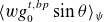 $\langle wg^{t,bp}_{0}\sin \theta \rangle _\psi$
does not jump across the trapped–barely passing region, and the second and fourth terms vanish when integrated over
$\langle wg^{t,bp}_{0}\sin \theta \rangle _\psi$
does not jump across the trapped–barely passing region, and the second and fourth terms vanish when integrated over $w$
. The third term is the only term that does not vanish. Thus, we find that
$w$
. The third term is the only term that does not vanish. Thus, we find that
 \begin{align} \bigg \langle\! \int \mathrm{d}^3v\:\varSigma \bigg \rangle _\psi =\frac {\partial \varGamma }{\partial \psi }, \end{align}
where
 \begin{align} \varGamma =-\,\bigg \langle\! \int _{V_{tbp}} \mathrm{d}^3v\:\frac {I}{\varOmega }\frac {1}{qR}\frac {r}{R}\mathcal{P}(\theta )g^{t,bp}_{0}\bigg \rangle _\psi \end{align}
is the ion neoclassical particle flux. We need to calculate $g^{t,bp}_{0}$
to evaluate this integral.
$g^{t,bp}_{0}$
to evaluate this integral.
Using the same manipulations that we used for the particle conservation equation, we find that the parallel momentum moment of $\mathcal{L}[g^{t,bp}]$
in the trapped–barely passing region is
$\mathcal{L}[g^{t,bp}]$
in the trapped–barely passing region is
 \begin{align} \bigg \langle\! \int _{V_{tbp}} \mathrm{d}^3v\: m(w-u)\mathcal{L}[g^{t,bp}]\bigg \rangle _\psi \simeq \bigg \langle mu\int _{V_{tbp}} \mathrm{d}^3v\:\frac {\partial }{\partial \psi }\left [\frac {I}{\varOmega }\frac {1}{qR}\frac {r}{R}\mathcal{P}(\theta )g^{t,bp}_{0}\right ]\bigg \rangle _\psi \nonumber \\[4pt] -\,\bigg \langle\! \int _{V_{tbp}} \mathrm{d}^3v\:mw\frac {S}{qR}\frac {r}{R}\frac {\partial }{\partial w} \big[\mathcal{P}(\theta )g^{t,bp}_{0}\big]\bigg \rangle _\psi . \end{align}
Note that the second term is the result of keeping the small difference between $v_\parallel$
and
$v_\parallel$
and $-u$
in (2.45). In (2.58) the particle moment of this term did not give a contribution, but here we need to keep it. We can integrate the second term in (2.62) by parts to relate it to the particle flux (2.61):
$-u$
in (2.45). In (2.58) the particle moment of this term did not give a contribution, but here we need to keep it. We can integrate the second term in (2.62) by parts to relate it to the particle flux (2.61):
 \begin{equation} \bigg \langle\! \int _{V_{tbp}} \mathrm{d}^3v\: m(w-u)\mathcal{L}[g^{t,bp}]\bigg \rangle _\psi \simeq -mu\frac {\partial \varGamma }{\partial \psi } -mS\frac {\varOmega }{I}\varGamma . \end{equation}
There was no jump term when we integrated by parts because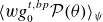 $\langle w g_0^{t,bp}\mathcal{P}(\theta )\rangle _\psi$
does not jump across the trapped–barely passing region for the same reason as argued below (2.59). Note that we have neglected the
$\langle w g_0^{t,bp}\mathcal{P}(\theta )\rangle _\psi$
does not jump across the trapped–barely passing region for the same reason as argued below (2.59). Note that we have neglected the $\theta$
dependence of
$\theta$
dependence of $u$
,
$u$
, $S$
and
$S$
and $\varOmega$
, which is small in
$\varOmega$
, which is small in $\epsilon$
. Going forward, we can drop all
$\epsilon$
. Going forward, we can drop all $\theta$
dependence in
$\theta$
dependence in $u$
,
$u$
, $S$
and
$S$
and $\varOmega$
. We can use (2.63) in the parallel momentum relation (2.53) and find the parallel momentum conservation equation
$\varOmega$
. We can use (2.63) in the parallel momentum relation (2.53) and find the parallel momentum conservation equation
 \begin{equation} \bigg \langle\! \int \mathrm{d}^3v\:mv_\parallel \varSigma \bigg \rangle _\psi =\frac {\partial }{\partial \psi }\left (-mu\varGamma \right )-m\frac {\varOmega }{I}\varGamma . \end{equation}
Finally, using again the same manipulations that we used for the particle and parallel momentum conservation equation, we find that the energy transport (2.56) is described by the equation
 \begin{align} \bigg \langle\! \int \mathrm{d}^3v\:\frac {mv^2}{2}\varSigma \bigg \rangle _\psi &=-\bigg \langle\! \int _{V_{tbp}} \mathrm{d}^3v\:\left (\frac {mu^2}{2}+m\mu B\right )\frac {\partial }{\partial \psi }\left [\frac {I}{\varOmega }\frac {1}{qR}\frac {r}{R}\mathcal{P}(\theta )g^{t,bp}_{0}\right ]\bigg \rangle _\psi \nonumber \\ & \quad -\bigg \langle\! \int _{V_{tbp}} \mathrm{d}^3v\:muw\frac {S}{qR}\frac {r}{R}\frac {\partial }{\partial w}\big[\mathcal{P}(\theta )g^{t,bp}_{0}\big]\bigg \rangle _\psi . \end{align}
The second term on the right-hand side is due to the small difference of $v_\parallel$
and
$v_\parallel$
and $-u$
in the trapped–barely passing region. We can integrate the second term by parts, because
$-u$
in the trapped–barely passing region. We can integrate the second term by parts, because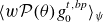 $\langle w \mathcal{P}(\theta )g_0^{t,bp}\rangle _\psi$
does not jump across the trapped–barely passing region, and relate it to the particle flux:
$\langle w \mathcal{P}(\theta )g_0^{t,bp}\rangle _\psi$
does not jump across the trapped–barely passing region, and relate it to the particle flux:
 \begin{align} \bigg \langle\! \int \mathrm{d}^3v\:\frac {mv^2}{2}\varSigma \bigg \rangle _\psi & =-\frac {\partial }{\partial \psi }\bigg \langle\! \int _{V_{tbp}} \mathrm{d}^3v\:\left (\frac {mu^2}{2}+m\mu B\right )\left [\frac {I}{\varOmega }\frac {1}{qR}\frac {r}{R}\mathcal{P}(\theta )g^{t,bp}_{0}\right ]\bigg \rangle _\psi \nonumber \\& \quad -mu\frac {\partial u}{\partial \psi }\varGamma +muS\frac {\varOmega }{I}\varGamma . \end{align}
The energy conservation (2.66) can be written as
 \begin{equation} \bigg \langle\! \int \mathrm{d}^3v\:\frac {mv^2}{2}\varSigma \bigg \rangle _\psi =\frac {\partial Q}{\partial \psi } +mu\frac {\varOmega }{I}\varGamma , \end{equation}
with the energy flux
 \begin{equation} Q= -\bigg \langle\! \int _{V_{tbp}} \mathrm{d}^3v\:\left (\frac {mu^2}{2}+m\mu B\right )\frac {I}{\varOmega }\frac {1}{qR}\frac {r}{R}\mathcal{P}(\theta )g^{t,bp}_{0}\bigg \rangle _\psi . \end{equation}
2.4. Electron neoclassical transport
The electron neoclassical transport relations can be derived following the exact same steps as for the ions. The main differences are that the square root of the mass ratio $\sqrt {m_e/m} \ll \epsilon \ll 1$
, where
$\sqrt {m_e/m} \ll \epsilon \ll 1$
, where $m_e$
is the electron mass, introduces a second small parameter and that electron–ion collisions must be kept in addition to electron–electron collisions. We showed in Trinczek et al. (Reference Trinczek, Parra and Catto2025, Equation (2.23)) that this leads to a collision operator where we can replace the term
$m_e$
is the electron mass, introduces a second small parameter and that electron–ion collisions must be kept in addition to electron–electron collisions. We showed in Trinczek et al. (Reference Trinczek, Parra and Catto2025, Equation (2.23)) that this leads to a collision operator where we can replace the term $\mathcal{\sf {M}}_\parallel$
by
$\mathcal{\sf {M}}_\parallel$
by
 \begin{equation} \mathcal{\sf {M}}_{\parallel e}=\frac {3}{2}\sqrt {\frac {\pi }{2}}\frac {T_e}{m_e}\frac {\nu _{ee}}{x_e}\left [\varTheta (x_e)-\varPsi (x_e)+Z\right ]\!. \end{equation}
Here, $T_e$
is the electron temperature,
$T_e$
is the electron temperature, $\nu _{ee}=4\sqrt {\pi }e^4n_e\log \varLambda /(3T_e^{3/2}m_e^{1/2})$
,
$\nu _{ee}=4\sqrt {\pi }e^4n_e\log \varLambda /(3T_e^{3/2}m_e^{1/2})$
, $n_e$
is the electron density and
$n_e$
is the electron density and $x_e=v/v_{te}$
, where
$x_e=v/v_{te}$
, where $v_{te}=\sqrt {2T_e/m_e}$
is the electron thermal speed. Note that the definition of
$v_{te}=\sqrt {2T_e/m_e}$
is the electron thermal speed. Note that the definition of $\nu _{ee}$
is consistent with the definition by Trinczek et al. (Reference Trinczek, Parra and Catto2025) (see text above (2.1) in that paper) but differs by a factor of
$\nu _{ee}$
is consistent with the definition by Trinczek et al. (Reference Trinczek, Parra and Catto2025) (see text above (2.1) in that paper) but differs by a factor of $\sqrt {2}$
from the standard Braginskii definition. Dropping terms that are small in mass ratio and using the fact that the electron charge is
$\sqrt {2}$
from the standard Braginskii definition. Dropping terms that are small in mass ratio and using the fact that the electron charge is $-e$
, we find the electron neoclassical particle flux, i.e.
$-e$
, we find the electron neoclassical particle flux, i.e.
 \begin{equation} \varGamma _e=-\,\bigg \langle\! \int _{V_{tbp}}\mathrm{d}^3v\:\frac {I}{\varOmega _e}\frac {1}{qR}\frac {r}{R}\mathcal{P}_e(\theta )g^{t,bp}_{e0}\bigg \rangle _\psi , \end{equation}
where $\varOmega _e=-eB/m_ec$
is the electron Larmor frequency and
$\varOmega _e=-eB/m_ec$
is the electron Larmor frequency and
 \begin{equation} \mathcal{P}_e(\theta )=\mu B\sin \theta -\frac {eR}{m_er}\frac {\partial \phi _\theta }{\partial \theta }. \end{equation}
The electron neoclassical energy flux is
 \begin{equation} Q_e= -\,\bigg \langle\! \int _{V_{tbp}} \mathrm{d}^3v\:m_e\mu B\frac {I}{\varOmega _e}\frac {1}{qR}\frac {r}{R}\mathcal{P}_{e}(\theta )g^{t,bp}_{e0}\bigg \rangle _\psi . \end{equation}
The bootstrap current can also be calculated from the electron distribution function. We follow the derivation for the bootstrap current in § 2.3 of Trinczek et al. (Reference Trinczek, Parra and Catto2025), but generalise it for $\nu _\ast \sim 1$
. The bootstrap current is defined as
$\nu _\ast \sim 1$
. The bootstrap current is defined as
 \begin{equation} j_\parallel ^B\equiv Ze\int \mathrm{d}^3v\: v_\parallel f - e\int \mathrm{d}^3v \: v_\parallel f_e=ZenV_\parallel -en_eV_{\parallel } -e\int \mathrm{d}^3v\: v_\parallel g_e. \end{equation}
Quasineutrality reduces this expression to
 \begin{equation} j_\parallel ^B=-e\int \mathrm{d}^3v \: v_\parallel g_{e}. \end{equation}
Using the same approach as Trinczek et al. (Reference Trinczek, Parra and Catto2025, § 2.3), we can use the Spitzer–Härm function in (2.74). The Spitzer–Härm function is defined to satisfy the property
 \begin{align} v_\parallel f_{Me}=C_e[f_{e,SH}] \end{align}
and is of the form
 \begin{align} f_{e,SH}=\frac {v_\parallel }{\sqrt {2}\nu _{ee}}f_{Me}A_{SH}\big(x_e^2\big), \end{align}
where
 \begin{align} A_{SH}\big(x_e^2\big)=\sum _i a_i L_i^{3/2}\big(x_e^2\big). \end{align}
Here, $L_i^{3/2}\big(x_e^2\big)$
are Laguerre polynomials and
$L_i^{3/2}\big(x_e^2\big)$
are Laguerre polynomials and $a_i$
are coefficients determined by (2.75). The first three coefficients for
$a_i$
are coefficients determined by (2.75). The first three coefficients for $Z=1$
are
$Z=1$
are $a_0=-1.975$
,
$a_0=-1.975$
, $a_1=0.558$
,
$a_1=0.558$
, $a_2=0.015$
. We use (2.75) in (2.74) to write the flux surface averaged bootstrap current as
$a_2=0.015$
. We use (2.75) in (2.74) to write the flux surface averaged bootstrap current as
 \begin{equation} \big\langle j_\parallel ^B\big\rangle _\psi =-e\Bigg \langle \int \mathrm{d}^3v\: \frac {g_{e}}{f_{Me}}C_e[f_{e,SH}]\Bigg \rangle _\psi =-e\Bigg \langle \int \mathrm{d}^3v\: \frac {f_{e,SH}}{f_{Me}}C_e[g_{e}]\Bigg \rangle _\psi , \end{equation}
where we have used the self-adjointness of the collision operator. The bootstrap current can be expressed as a moment of the collision operator,
 \begin{equation} \big\langle j_\parallel ^B\big\rangle _\psi \simeq -\Bigg \langle \int \mathrm{d}^3v\: \frac {e}{\sqrt {2}\nu _{ee}} v_\parallel A_{SH} C_e[g_e]\Bigg \rangle _\psi . \end{equation}
At this point, we can employ (2.20),
 \begin{align} \big\langle j_\parallel ^B\big\rangle _\psi &\simeq -\Bigg \langle \int _{V_{tbp}}\mathrm{d}^3v\: \frac {e}{\sqrt {2}\nu _{ee}} v_\parallel A_{SH} \mathcal{L}[g_e^{t,bp}]\Bigg \rangle _\psi \nonumber \\ & \simeq \Bigg \langle \int _{V_{tbp}}\mathrm{d}^3v\: \frac {e}{\sqrt {2}\nu _{ee}} w A_{SH} \frac {1}{qR}\frac {r}{R}\frac {\partial }{\partial w} \big[\mathcal{P}_e(\theta )g^{t,bp}_{e0}\big]\Bigg \rangle _\psi . \end{align}
Upon integration by parts, where we use the fact that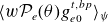 $\langle w\mathcal{P}_e(\theta )g_{e0}^{t,bp}\rangle _\psi$
does not jump across the trapped–barely passing region as argued below (2.59) and
$\langle w\mathcal{P}_e(\theta )g_{e0}^{t,bp}\rangle _\psi$
does not jump across the trapped–barely passing region as argued below (2.59) and $x_e^2\simeq m_e\mu B/T_e$
, the bootstrap current is given by
$x_e^2\simeq m_e\mu B/T_e$
, the bootstrap current is given by
 \begin{equation} \big\langle j_\parallel ^B\big\rangle _\psi =-\bigg \langle\! \int _{V_{tbp}}\mathrm{d}^3v\: \frac {e}{\sqrt {2}\nu _{ee}}A_{SH}\frac {1}{qR}\frac {r}{R}\mathcal{P}_e(\theta )g_{e0}^{t,bp}\bigg \rangle _\psi . \end{equation}
All results up to this point are valid to lowest order in $\sqrt {\epsilon }$
and
$\sqrt {\epsilon }$
and $\nu _\ast \sim 1$
for asymptotically small
$\nu _\ast \sim 1$
for asymptotically small $\epsilon$
. When
$\epsilon$
. When $\epsilon$
is a small but finite number, this approach breaks down when
$\epsilon$
is a small but finite number, this approach breaks down when $\nu _\ast \gtrsim \epsilon ^{-3/2}$
because a distinction between trapped–barely passing and freely passing particles is no longer possible. To calculate the particle flux and the energy flux, it is necessary to distinguish between the different collisionality regimes. The calculation for the banana regime,
$\nu _\ast \gtrsim \epsilon ^{-3/2}$
because a distinction between trapped–barely passing and freely passing particles is no longer possible. To calculate the particle flux and the energy flux, it is necessary to distinguish between the different collisionality regimes. The calculation for the banana regime, $\nu _\ast \ll 1$
, was carried out in Trinczek et al. (Reference Trinczek, Parra, Catto, Calvo and Landreman2023). We present the derivation for the plateau regime,
$\nu _\ast \ll 1$
, was carried out in Trinczek et al. (Reference Trinczek, Parra, Catto, Calvo and Landreman2023). We present the derivation for the plateau regime, $\epsilon ^{-3/2}\gg \nu _\ast \gg 1$
, in the next section.
$\epsilon ^{-3/2}\gg \nu _\ast \gg 1$
, in the next section.
3. Plateau regime
The plateau regime is defined by
 \begin{equation} 1\ll \nu _\ast \ll \epsilon ^{-3/2} \quad \mbox{and }\quad \epsilon \ll 1. \end{equation}
The collision frequency is small compared with the bounce frequency of freely passing particles but big enough that trapped and barely passing particles collide many times before they can complete their orbits. Hence, we will refer to the particles with small $w$
as being in a collisional layer of a width that we determine in a few lines, and refrain from distinguishing trapped and barely passing particles. The distribution function in this collisional layer is called
$w$
as being in a collisional layer of a width that we determine in a few lines, and refrain from distinguishing trapped and barely passing particles. The distribution function in this collisional layer is called $g^l$
and replaces the distribution function
$g^l$
and replaces the distribution function $g^{t,bp}$
. The width of the collisional layer in
$g^{t,bp}$
. The width of the collisional layer in $w$
is determined by imposing that the effective collision frequency
$w$
is determined by imposing that the effective collision frequency $\nu v_{t}^2/w^2$
be comparable to the time it takes a particle to complete one full poloidal turn,
$\nu v_{t}^2/w^2$
be comparable to the time it takes a particle to complete one full poloidal turn,
 \begin{equation} \frac {w}{qR}\sim \nu \frac {v^2_t}{w^2} \end{equation}
and, hence, the width of the collisional layer is
 \begin{equation} \frac {w}{v_{t}}\sim \left (\frac {qR\nu }{v_{t}}\right )^{1/3}\sim \epsilon ^{1/2}\nu _\ast ^{1/3}. \end{equation}
3.1. Ion transport in the plateau regime
In order to determine $g^l_0$
in the plateau regime, we can use the fact that the second term on the left-hand side of (2.32), the term proportional to
$g^l_0$
in the plateau regime, we can use the fact that the second term on the left-hand side of (2.32), the term proportional to $\partial g_0^l/\partial w$
, is smaller than other terms that contain
$\partial g_0^l/\partial w$
, is smaller than other terms that contain $g^l_{0}$
by
$g^l_{0}$
by $1/\nu _\ast ^{2/3}\ll 1$
, due to (3.3). Thus, (2.32) simplifies to
$1/\nu _\ast ^{2/3}\ll 1$
, due to (3.3). Thus, (2.32) simplifies to
 \begin{equation} \frac {\partial }{\partial \theta }\left (\frac {w}{qR}g^l_{0}\right )-\mathsf{M}_\parallel \frac {\partial ^2{g^l_{0}}}{\partial {w}^2}=\frac {I}{\varOmega }\mathcal{P}(\theta )\frac {r}{R}\frac {1}{qR} \mathcal{D}f_M. \end{equation}
It follows from this equation that the lowest order correction to the distribution function in the plateau regime must be of the size $g^l_{0}/f_M\sim \epsilon ^{1/2}/\nu _\ast ^{1/3}\ll 1$
. Equation (3.4) is analytically solvable if the
$g^l_{0}/f_M\sim \epsilon ^{1/2}/\nu _\ast ^{1/3}\ll 1$
. Equation (3.4) is analytically solvable if the $\theta$
dependence of
$\theta$
dependence of $u$
and
$u$
and $\varOmega$
is neglected as small in
$\varOmega$
is neglected as small in $\epsilon$
and the form of the potential is taken to be
$\epsilon$
and the form of the potential is taken to be
 \begin{equation} \phi _\theta =\phi _c(\psi )\cos \theta +\phi _s(\psi )\sin \theta . \end{equation}
This choice will be justified for concentric circular flux surfaces in the calculation of the electric potential in § 3.3. Introducing the amplitudes
 \begin{align} A_S\equiv u^2+\mu B-\frac {Ze\phi _c R}{mr}, && A_C\equiv \frac {Ze\phi _sR}{m r}, \end{align}
we can write
 \begin{equation} \mathcal{P}(\theta )=A_S\sin \theta +A_C\cos \theta \end{equation}
in (3.4). The full derivation of the solution to (3.4) is in Appendix B, which follows Su & Oberman (Reference Su and Oberman1968). The solution is
 \begin{equation} g^l_{0}=\left [A_SF_s(\xi ,\theta )+A_CF_c(\xi ,\theta )\right ]\frac {I}{\varOmega } \frac {\mathcal{D}}{v_{\textrm {ref}}}\frac {r}{R} f_M(w=0), \end{equation}
where $\xi =w/v_{\textrm {ref}}$
,
$\xi =w/v_{\textrm {ref}}$
, $v_{\textrm {ref}}=(qR\mathsf{M}_\parallel )^{1/3}$
,
$v_{\textrm {ref}}=(qR\mathsf{M}_\parallel )^{1/3}$
,
 \begin{equation} F_s(\xi ,\theta )=\int _0^\infty \mathrm{d}p \:\exp \left (-\frac {p^3}{3}\right )\sin (\theta -p\xi ) \end{equation}
and
 \begin{equation} F_c(\xi ,\theta )=\int _0^\infty \mathrm{d}p\:\exp \left (-\frac {p^3}{3}\right )\cos (\theta -p\xi ). \end{equation}
Importantly, $\langle g^l_{0}\rangle _\tau =0$
and
$\langle g^l_{0}\rangle _\tau =0$
and $g^l_{0}$
matches (2.28) for
$g^l_{0}$
matches (2.28) for $\xi \rightarrow \infty$
, a result demonstrated in Appendix B. We also need the integral
$\xi \rightarrow \infty$
, a result demonstrated in Appendix B. We also need the integral
 \begin{equation} \lim _{W\rightarrow \infty } \int _{-W}^{W}\text{d}w\:g^l_{0}=\frac {{\pi}I}{\varOmega }\frac {r}{R}\mathcal{D}\left (A_C\cos \theta +A_S\sin \theta \right )f_M(w=0) \end{equation}
to calculate the particle flux $\varGamma$
in (2.61). The derivation of (3.11) is presented in Appendix B.
$\varGamma$
in (2.61). The derivation of (3.11) is presented in Appendix B.
We can use (3.11) in (2.61) to find the ion neoclassical particle flux, i.e.
 \begin{equation} \varGamma =-\frac {BI^2\pi ^2}{qR\varOmega ^2}\left (\frac {r}{R}\right )^2\int \text{d}\mu \left (A_S^2+A_C^2\right )\mathcal{D}f_M(w=0), \end{equation}
where we also carried out the flux surface average. The integration over $\mu$
gives
$\mu$
gives
 \begin{align} \varGamma & =-\frac {\sqrt {\pi }}{4}\frac {n}{qR}\frac {I^2}{\varOmega ^2}\left (\frac {r}{R}\right )^2\left (\frac {2T}{m}\right )^{3/2}\exp \left (-\frac {m(u+V_\parallel )^2}{2T}\right )\nonumber \\[4pt] & \quad \times \Bigg \lbrace \frac {1}{2}\left [\left (\frac {mu^2}{T}-\frac {ZeR\phi _c}{Tr}\right )^2+\left (\frac {ZeR\phi _s}{Tr}\right )^2\right ]\mathcal{D}_{-3/2} +\left (\frac {mu^2}{T}-\frac {ZeR}{Tr}\phi _c\right )\mathcal{D}_{-1/2}+\mathcal{D}_{1/2}\Bigg \rbrace .\nonumber\\[2pt] \end{align}
Here, we have introduced the notation,
 \begin{equation} \mathcal{D}_l\equiv \frac {\partial }{\partial \psi }\ln p-\frac {m(u+V_\parallel )}{T}\left (\frac {\partial V_\parallel }{\partial \psi }-\frac {\varOmega }{I}\right )+\left [\frac {m(u+V_\parallel )^2}{2T}+l\right ]\frac {\partial }{\partial \psi }\ln T, \end{equation}
where $l$
is a rational number.
$l$
is a rational number.
The energy flux $Q$
in (2.68) is
$Q$
in (2.68) is
 \begin{equation} Q=-\frac {BTI^2\pi ^2}{qR\varOmega ^2}\left (\frac {r}{R}\right )^2\int \text{d}\mu \:\left (\frac {mu^2}{2T}+\frac {m \mu B}{T}\right )\left (A_S^2+A_C^2\right )\mathcal{D}f_M(w=0), \end{equation}
which can be calculated to give
 \begin{align} Q & = \frac {mu^2}{2}\varGamma _i-\frac {3\sqrt {\pi }}{4}\frac {nT}{qR}\frac {I^2}{\varOmega ^2 }\left (\frac {r}{R}\right )^2 \left (\frac {2T}{m}\right )^{3/2}\exp \left (-\frac {m(u+V_\parallel )^2}{2T}\right )\nonumber \\& \quad\times \Bigg \lbrace \frac {1}{6}\left [\left (\frac {mu^2}{T}-\frac {Ze\phi _c R}{Tr}\right )^2 + \left (\frac {Ze\phi _s R}{Tr}\right )^2\right ]\mathcal{D}_{-1/2}\nonumber \\ & \qquad\qquad +\frac {2}{3}\left (\frac {mu^2}{T}-\frac {Ze\phi _cR}{Tr}\right )\mathcal{D}_{1/2}+\mathcal{D}_{3/2}\Bigg \rbrace . \end{align}
In the limit of weak gradients, the poloidal variation vanishes, and the neoclassical ion particle flux (3.13) and energy flux (3.16) agree with the results of weak gradient neoclassical theory, as shown in Appendix C.
We compare the results in (3.13) and (3.16) to previous work on strong gradient neoclassical transport in the plateau regime by Pusztai & Catto (Reference Pusztai and Catto2010) and Seol & Shaing (Reference Seol and Shaing2012) in Appendix D, and find that our results disagree due to inconsistencies in previous work.
3.2. Electron transport in the plateau regime
The electron distribution function $g^l_{e0}$
can be derived following the exact same steps as for the ion distribution function. The result is
$g^l_{e0}$
can be derived following the exact same steps as for the ion distribution function. The result is
 \begin{equation} g^l_{e0}=\left [A_{Se}F_s(\xi _e,\theta )+A_{Ce}F_c(\xi _e,\theta )\right ]\frac {I}{\varOmega _e} \frac {\mathcal{D}_e}{v_{\textrm {ref,e}}}\frac {r}{R} f_{Me}(v_\parallel =0), \end{equation}
where $\xi _e=v_\parallel /v_{\textrm {ref,e}}$
,
$\xi _e=v_\parallel /v_{\textrm {ref,e}}$
, $v_{\textrm {ref,e}}=(qR\mathsf{M}_{\parallel e})^{1/3}$
,
$v_{\textrm {ref,e}}=(qR\mathsf{M}_{\parallel e})^{1/3}$
,
 \begin{align} A_{Se}=\mu B+\frac {e\phi _c R}{m_e r}, \qquad \qquad \qquad \qquad A_{Ce}=-\frac {e\phi _sR}{m_er}, \\[-12pt]\nonumber \end{align}
 \begin{align} \mathcal{D}_e=\frac {\partial }{\partial \psi }\ln {p_e} +\frac {m_e(u+ V_\parallel )}{T}\frac {\varOmega _e}{I} +\left (\frac {m_e\mu B}{T_e}-\frac {5}{2}\right )\frac {\partial }{\partial \psi }\ln {T_e} \end{align}
and $p_e=n_eT_e$
is the electron pressure. We can use the distribution function (3.17) in (2.70) and integrate to find that
$p_e=n_eT_e$
is the electron pressure. We can use the distribution function (3.17) in (2.70) and integrate to find that
 \begin{align} \varGamma _e=-\frac {\sqrt {\pi }}{4}\frac {n_e}{qR}\frac {I^2}{\varOmega _e^2}\left (\frac {r}{R}\right )^2\left (\frac {2T_e}{m_e}\right )^{3/2} &\Bigg \lbrace \frac {1}{2}\left [\left (\frac {e\phi _cR}{T_er}\right )^2+\left (\frac {e\phi _s R}{T_e r}\right )^2\right ]\mathcal{D}_{e,-3/2}\nonumber \\ & \quad \, +\frac {e\phi _c R}{T_e r}\mathcal{D}_{e,-1/2}+\mathcal{D}_{e,1/2}\Bigg \rbrace , \end{align}
where
 \begin{equation} \mathcal{D}_{e,l}\equiv \frac {\partial }{\partial \psi }\ln p_e+\frac {m_e(u+V_\parallel )}{T_e}\frac {\varOmega _e}{I}+l\frac {\partial }{\partial \psi }\ln T_e. \end{equation}
Similarly, the electron energy flux (2.72) yields
 \begin{align} Q_e=-\frac {3\sqrt {\pi }}{4}\frac {n_eT_e}{qR}\frac {I^2}{\varOmega _e^2}\left (\frac {r}{R}\right )^2\left (\frac {2T_e}{m_e}\right )^{3/2} &\Bigg \lbrace \frac {1}{6}\left [\left (\frac {e\phi _cR}{T_er}\right )^2 +\left (\frac {e\phi _s R}{T_e r}\right )^2\right ]\mathcal{D}_{e,-1/2}\nonumber \\ &\qquad \qquad +\frac {2}{3}\frac {e\phi _c R}{T_e r}\mathcal{D}_{e,1/2}+\mathcal{D}_{e,3/2}\Bigg \rbrace . \end{align}
In the limit of weak gradients, the neoclassical electron particle flux (3.20) and energy flux (3.22) agree with the results of weak gradient neoclassical theory, as shown in Appendix C.
We can insert the electron distribution function (3.17) in (2.81) to calculate the bootstrap current. We take the integral (2.81) by using properties of the Laguerre polynomials. The derivation is shown in detail in Appendix E. The final result for the bootstrap current reads
 \begin{align} \big\langle j_\parallel ^B\big\rangle _\psi &= -\frac {1}{8}\sqrt {\frac {\pi }{2}}\frac {en_e}{\nu _{ee}qR}\frac {I}{\varOmega _e}\left (\frac {r}{R}\right )^2\left (\frac {2T_e}{m_e}\right )^{3/2}\Bigg \lbrace \left [\left (\frac {e\phi _cR}{T_er}\right )^2+\left (\frac {e\phi _sR}{T_er}\right )^2\right ]\nonumber \\[4pt] &\quad \times \sum _{i=0} \frac {2a_i\varGamma (i+ {3}/{2})}{\sqrt {\pi }\varGamma (1+i)}\mathcal{D}_{e,\alpha _i} +2\frac {e\phi _cR}{T_e r}\left [a_0\mathcal{D}_{e,-({1}/{2})}+\sum _{i=1}\frac {a_i\varGamma (i+ {1}/{2})}{\sqrt {\pi }\varGamma (1+i)}\mathcal{D}_{e,\beta _i}\right ]\nonumber \\[4pt] &\quad +\left [2a_0\mathcal{D}_{e,1/2}-a_1\mathcal{D}_{e,13/2}-\sum _{i=2} \frac {a_i\varGamma (i-{1}/{2})}{\sqrt {\pi }\varGamma (1+i)} \mathcal{D}_{e,\gamma _i} \right ]\Bigg \rbrace , \end{align}
where
 \begin{align} \alpha _i=-\frac {3/2+5i}{1+2i},&&\beta _i=\frac {1-10i}{4i-2},&&\gamma _i=-\frac {(3+10i)(i-1/2)}{4}. \end{align}
Note that $\varGamma$
here is the Euler Gamma function and not the particle flux. The result agrees with the weak gradient limit in Appendix C and we compare it to previous results by Pusztai & Catto (Reference Pusztai and Catto2010) in Appendix D.
$\varGamma$
here is the Euler Gamma function and not the particle flux. The result agrees with the weak gradient limit in Appendix C and we compare it to previous results by Pusztai & Catto (Reference Pusztai and Catto2010) in Appendix D.
3.3. Electric potential
The calculation of the electric potential in the plateau regime follows the derivation in the banana regime in § 4.4 of Trinczek et al. (Reference Trinczek, Parra, Catto, Calvo and Landreman2023). We assume a Boltzmann response for the electrons such that quasineutrality reads
 \begin{equation} Zn_\theta =\frac {en_e}{T_e}\phi _\theta . \end{equation}
The poloidal density variation as derived in Trinczek et al. (Reference Trinczek, Parra, Catto, Calvo and Landreman2023, Equation (4.56)) is
 \begin{equation} n_\theta =\lim _{W\rightarrow \infty }\int _0^\infty \mathrm{d}\mu \int _{-W}^W\mathrm{d}w\: 2\pi B (g^l-\langle g^l\rangle _\psi )+\int _{V_p}\mathrm{d}^3v \:2\pi B(g^p-\langle g^p\rangle _\psi ) \equiv n_\theta ^l+n_\theta ^p, \end{equation}
where the integration is performed over both the collisional layer and the freely passing region of velocity space, and hence, one must calculate the contributions from $g^l$
and
$g^l$
and $g^p$
separately. The freely passing particle contribution is the same as in the banana regime. The distribution function
$g^p$
separately. The freely passing particle contribution is the same as in the banana regime. The distribution function $g^p$
diverges as
$g^p$
diverges as $v_\parallel \rightarrow -u$
; see (2.28). This divergence is compensated for by the contribution from the collisional layer. We comment on the validity of this integration in Appendix B.2. The freely passing particle contribution was calculated by Trinczek et al. (Reference Trinczek, Parra, Catto, Calvo and Landreman2023) in their equation (4.57) and yields
$v_\parallel \rightarrow -u$
; see (2.28). This divergence is compensated for by the contribution from the collisional layer. We comment on the validity of this integration in Appendix B.2. The freely passing particle contribution was calculated by Trinczek et al. (Reference Trinczek, Parra, Catto, Calvo and Landreman2023) in their equation (4.57) and yields
 \begin{align} n_\theta ^p & =- n\frac {Ir}{\varOmega R}\Bigg \lbrace \sqrt {\frac {2T}{m}}J \bigg [\left (\frac {mV_\parallel ^2}{T}\cos \theta +\cos \theta -\frac {Ze\phi _\theta R}{Tr}\right )\left (\frac {\partial }{\partial \psi }\ln p-\frac {3}{2}\frac {\partial }{\partial \psi }\ln T\right )\nonumber \\ &\quad +\cos \theta \frac {\partial }{\partial \psi }\ln T \bigg ] +\left [1-2\sqrt {\frac {m}{2T}}(V_\parallel +u)J\right ]\Bigg \lbrace (V_\parallel -u)\cos \theta \left (\frac {\partial }{\partial \psi }\ln p-\frac {3}{2}\frac {\partial }{\partial \psi }\ln T\right )\nonumber \\ &\quad -(V_\parallel +u)\Bigg [\left (\frac {mV_\parallel ^2}{2T}+\frac {1}{2}\right )\cos \theta -\frac {Ze\phi _\theta R}{2Tr}\Bigg ]\frac {\partial }{\partial \psi }\ln T+\left (\frac {\partial V_\parallel }{\partial \psi }-\frac {\varOmega }{I}\right )\nonumber \\ &\quad \times \left [\left (\frac {m u^2}{T}+1-\frac {m(V_\parallel +u)^2}{T}\right )\cos \theta -\frac {Ze\phi _\theta R}{Tr}\right ]\Bigg \rbrace \nonumber \\ &\quad +\left [1+2\frac {m(V_\parallel +u)^2}{2T}-4\left (\frac {m}{2T}\right )^{3/2}(V_\parallel +u)^3J\right ]\cos \theta \!\left (\frac {\partial V_\parallel }{\partial \psi }-\frac {\varOmega }{I}+\frac {V_\parallel -u}{2}\frac {\partial }{\partial \psi }\ln T\right )\!\Bigg \rbrace \nonumber \\ &\hspace{23.5pc}-2n\frac {r}{R}\cos \theta , \end{align}
where $J$
is defined as
$J$
is defined as
 \begin{equation} J=\frac {\sqrt {\pi } }{2}\exp \left (-\frac {m(u+V_\parallel )^2}{2T}\right )\textrm {erfi}\left (\sqrt {\frac {m}{2T}}(u+V_\parallel )\right )\!. \end{equation}
Note that the dependence on $\cos \theta$
in this expression is coming from the magnetic field strength. We provide additional comments on the derivation of (3.27) and (3.28) in Appendix B.3.
$\cos \theta$
in this expression is coming from the magnetic field strength. We provide additional comments on the derivation of (3.27) and (3.28) in Appendix B.3.
In the banana regime the contribution from trapped and barely passing particles to the density vanishes because the $\theta$
-dependent part of the distribution function is odd in
$\theta$
-dependent part of the distribution function is odd in $w$
. In the plateau regime the contribution from the particles in the collisional layer does not vanish to lowest order. The term
$w$
. In the plateau regime the contribution from the particles in the collisional layer does not vanish to lowest order. The term $\int \text{d}\mu \int \text{d}w\:2\pi B g^l_{0}$
needs to be evaluated, whereas
$\int \text{d}\mu \int \text{d}w\:2\pi B g^l_{0}$
needs to be evaluated, whereas $\langle g^l_{0}\rangle _\tau$
vanishes. The velocity integration of
$\langle g^l_{0}\rangle _\tau$
vanishes. The velocity integration of $g^l_{0}$
can be performed using the solution for
$g^l_{0}$
can be performed using the solution for $g^l_{0}$
, (3.8), the relation (3.11) and assuming (3.5):
$g^l_{0}$
, (3.8), the relation (3.11) and assuming (3.5):
 \begin{align} n^l_\theta \simeq& \lim _{W\rightarrow \infty }\int _0^\infty \text{d}\mu \int _{-W}^W\text{d}w \: 2\pi B g^l_{0}= n\sqrt {\frac {m}{T}}\sqrt {\frac {\pi }{2}}\exp \left (-\frac {m(u+V_\parallel )^2}{2T}\right )\nonumber \\[4pt] &\times \Bigg \lbrace \frac {I}{\varOmega }\Bigg [\frac {Ze}{m}\phi _s\cos \theta +\left (u^2\frac {r}{R}-\frac {Ze}{m}\phi _c\right )\sin \theta \Bigg ] \mathcal{D}_{-3/2}+\frac {ITr}{\varOmega m R}\sin \theta \mathcal{D}_{-1/2}\Bigg \rbrace .\nonumber\\[3pt] \end{align}
Combining (3.27) and (3.29) in (3.25) yields an equation for the poloidally varying component of the electric potential $\phi _\theta =\phi _c(\psi )\cos \theta +\phi _s(\psi )\sin \theta$
. The terms proportional to
$\phi _\theta =\phi _c(\psi )\cos \theta +\phi _s(\psi )\sin \theta$
. The terms proportional to $\cos \theta$
give
$\cos \theta$
give
 \begin{align} \Bigg \lbrace \frac {en_e}{T_e} & -\frac {Z^2enI}{T\varOmega }\left[\sqrt {\frac {2T}{m}}J\left (\frac {\partial }{\partial \psi }\ln p-\frac {3}{2}\frac {\partial }{\partial \psi } \ln T\right )+\left [1-2\sqrt {\frac {m}{2T}}(V_\parallel +u) J\right ]\left(\frac {\partial V_\parallel }{\partial \psi }-\frac {\varOmega }{I}\right.\right.\nonumber \\ &\quad \left.\left.-\frac {(V_\parallel +u)}{2}\frac {\partial }{\partial \psi }\ln T\right)\right] \Bigg \rbrace \phi _c=-Zn\frac {Ir}{\varOmega R}\Bigg \lbrace \sqrt {\frac {2T}{m}}J\bigg [\left (\frac {mV_\parallel ^2}{T}+1\right )\nonumber \\ &\quad\times \left (\frac {\partial }{\partial \psi }\ln p-\frac {3}{2}\frac {\partial }{\partial \psi } \ln T\right )+\frac {\partial }{\partial \psi }\ln T\bigg ] +\left [1-2\sqrt {\frac {m}{2T}}(V_\parallel +u) J\right ]\nonumber \\ &\quad \times \bigg [(V_\parallel -u)\left (\frac {\partial }{\partial \psi }\ln p-\frac {3}{2}\frac {\partial }{\partial \psi }\ln T\right )+\left (\frac {\partial V_\parallel }{\partial \psi }-\frac {\varOmega }{I}\right )\left (\frac {mu^2}{T}+1-\frac {m(V_\parallel +u)^2}{T}\right )\nonumber \\ &\quad-\frac {V_\parallel +u}{2}\left (\frac {mV_\parallel ^2}{T}+1\right )\frac {\partial }{\partial \psi }\ln T\bigg ]\nonumber \\ &\quad +\left [1+\frac {m}{T}(V_\parallel +u)^2-4\left (\frac {m}{2T}\right )^{3/2}\left (V_\parallel +u\right )^3 J\right ]\left (\frac {\partial V_\parallel }{\partial \psi }-\frac {\varOmega }{I}+\frac {V_\parallel -u}{2}\frac {\partial }{\partial \psi }\ln T\right )\Bigg \rbrace \nonumber \\ &\quad+Zn\sqrt {\frac {m}{T}}\sqrt {\frac {\pi }{2}}\exp \left (-\frac {m(u+V_\parallel )^2}{2T}\right )\frac {Ze}{m}\phi _s \mathcal{D}_{-3/2}-2Zn\frac {r}{R}, \end{align}
and all terms proportional to $\sin \theta$
give
$\sin \theta$
give
 \begin{align} \Bigg \lbrace \frac {en_e}{T_e} & -\frac {Z^2enI}{T\varOmega }\bigg [\sqrt {\frac {2T}{m}}J\left (\frac {\partial }{\partial \psi }\ln p-\frac {3}{2}\frac {\partial }{\partial \psi } \ln T\right )+\left [1-2\sqrt {\frac {m}{2T}}(V_\parallel +u)J\right ]\nonumber \\[3pt]& \times \left(\frac {\partial V_\parallel }{\partial \psi }-\frac {\varOmega }{I}-\frac {V_\parallel +u}{2}\frac {\partial }{\partial \psi }\ln T\right)\bigg ] \Bigg \rbrace \phi _s=Zn\sqrt {\frac {m}{T}}\sqrt {\frac {\pi }{2}}\exp \left (-\frac {m(u+V_\parallel )^2}{2T}\right )\nonumber \\[3pt] & \times \Bigg [ \frac {I}{\varOmega }\left (u^2\frac {r}{R}-\frac {Ze}{m}\phi _c\right )\mathcal{D}_{-3/2} +\frac {TIr}{m\varOmega R}\mathcal{D}_{-1/2}\Bigg ] . \end{align}
Equations (3.30) and (3.31) form a linear system that can be solved for $\phi _c$
and
$\phi _c$
and $\phi _s$
. This result is consistent with our choice of
$\phi _s$
. This result is consistent with our choice of $\phi _\theta$
in (3.5).
$\phi _\theta$
in (3.5).
The usual neoclassical results for the electric potential can be retrieved by taking the limit $u\ll v_{t}$
,
$u\ll v_{t}$
, $V_\parallel \ll v_{t}$
and weak gradients. In this weak gradient limit, (3.30) and (3.31) reduce to
$V_\parallel \ll v_{t}$
and weak gradients. In this weak gradient limit, (3.30) and (3.31) reduce to
 \begin{align} \phi _c=0 \end{align}
and
 \begin{align} \left ( \frac {en_e}{T_e}+\frac {Z^2en}{T}\right )\phi _s =Zn\sqrt {\frac {T}{m}}\sqrt {\frac {\pi }{2}} \frac {Ir}{\varOmega R}\left [\frac {\partial }{\partial \psi }\ln p+\frac {m(u+V_\parallel )}{T}\frac {\varOmega }{I}-\frac {1}{2}\frac {\partial }{\partial \psi }\ln T\right ]\!.\nonumber\\[3pt] \end{align}
The vanishing parallel friction force in the weak gradient limit gives a relation for the mean parallel flow (C3), which can be used to simplify (3.33) to
 \begin{equation} \left ( \frac {en_e}{T_e}+\frac {Z^2en}{T}\right )\phi _s =-Zn\sqrt {\frac {T}{m}}\sqrt {\frac {\pi }{2}} \frac {Ir}{\varOmega R}\frac {\partial }{\partial \psi }\ln T. \end{equation}
A non-vanishing up–down asymmetry is consistent with the results of Hinton & Rosenbluth (Reference Hinton and Rosenbluth1973).
4. Case study
For a given set of input profiles for $n$
,
$n$
, $T$
,
$T$
, $T_e$
and
$T_e$
and $V_\parallel$
, we can calculate the transport fluxes
$V_\parallel$
, we can calculate the transport fluxes $\varGamma$
,
$\varGamma$
, $\varGamma _e$
,
$\varGamma _e$
, $Q$
and
$Q$
and $Q_e$
, the bootstrap current
$Q_e$
, the bootstrap current $\big\langle j_\parallel ^B\big\rangle _\psi$
, as well as the poloidal variation amplitudes
$\big\langle j_\parallel ^B\big\rangle _\psi$
, as well as the poloidal variation amplitudes $\phi _c$
and
$\phi _c$
and $\phi _s$
. We introduce normalised quantities, which are denoted by a bar,
$\phi _s$
. We introduce normalised quantities, which are denoted by a bar,
 \begin{align} \bar {\varGamma }=\varGamma \left (\frac {2p_0}{m}\frac {I\epsilon ^2}{qR\varOmega }\right )^{-1}, && \bar {\gamma }=\bigg \langle\! \int \mathrm{d}^3v\:mv_\parallel \varSigma \bigg \rangle _\psi \left (2p_0\frac {\epsilon ^2}{qR}\right )^{-1},\nonumber \\ \bar {Q}=Q\left (\frac {2p_0T_0}{m}\frac {I\epsilon ^2}{qR\varOmega }\right )^{-1},&& \bar {\varGamma }_e=\varGamma _e\left (\frac {2Zp_0}{m_e}\frac {I\epsilon ^2}{qR|\varOmega _e|}\sqrt {\frac {m_e}{m}}\right )^{-1},\nonumber \\ \bar {Q}_e=Q_e\left (\frac {2Zp_0T_0}{m_e}\frac {I\epsilon ^2}{qR|\varOmega _e|}\sqrt {\frac {m_e}{m}}\right )^{-1}, && \bar {j}^B=\big\langle j_\parallel ^B\big\rangle _\psi \left (\frac {2p_0}{m_e}\epsilon ^2 \frac {e}{qR\nu _{ee,0}}\sqrt {\frac {m_e}{m}}\right )^{-1}, \end{align}
where $T_0$
and
$T_0$
and $n_0$
are the values of density and temperature at a given point and
$n_0$
are the values of density and temperature at a given point and $p_0\equiv n_0T_0$
. Furthermore, we define
$p_0\equiv n_0T_0$
. Furthermore, we define
 \begin{align} \bar {u}\equiv \sqrt {\frac {m}{2T_0}}u,&\quad \bar {V}\equiv \sqrt {\frac {m}{2T_0}}V_\parallel , \quad \bar {\phi }_c\equiv \frac {ZeR\phi _c}{T_0r}, \quad \bar {\phi }_s\equiv \frac {ZeR\phi _s}{T_0r}, \quad \bar {E}_r\equiv -\bar {u}, \\[-12pt]\nonumber \end{align}
 \begin{align} \bar {T}\equiv \frac {T}{T_0},&\quad \bar {T}_e\equiv \frac {T_e}{T_0}, \quad \bar {n}\equiv \frac {n}{n_0}, \quad \bar {n}_e\equiv \frac {n_e}{Zn_0} \quad \frac {\partial }{\partial \bar {\psi }}\equiv \frac {I}{\varOmega }\sqrt {\frac {2T_0}{m}}\frac {\partial }{\partial \psi }, \\[-12pt]\nonumber\end{align}
 \begin{align} &\bar {\mathcal{D}}_{e,l}\equiv \frac {I}{\varOmega }\sqrt {\frac {2T_0}{m}} \mathcal{D}_{e,l}= \frac {\partial }{\partial \bar {\psi }}\ln \bar {p}_e-2\frac {\bar {u}+\bar {V}}{Z\bar {T}_e}+l\frac {\partial }{\partial \bar {\psi }}\ln \bar {T}_e \end{align}
and
 \begin{equation} \bar {\mathcal{D}}_l\equiv \frac {I}{\varOmega }\sqrt {\frac {2T_0}{m}} \mathcal{D}_l= \frac {\partial }{\partial \bar {\psi }}\ln \bar {p}-2\frac {\bar {u}+\bar {V}}{\bar {T}}\left (\frac {\partial \bar {V}}{\partial \bar {\psi }}-1\right )+\left [\frac {(\bar {u}+\bar {V})^2}{\bar {T}}+l\right ]\frac {\partial }{\partial \bar {\psi }}\ln \bar {T}, \end{equation}
where $l$
is a rational number.
$l$
is a rational number.
Using these definitions, the neoclassical ion particle flux (3.13) is
 \begin{align} \bar {\varGamma } & =-\frac {\sqrt {\pi }\bar {n}\bar {T}^{3/2}}{4}\exp \left [-\frac {(\bar {u}+\bar {V})^2}{\bar {T}}\right ] \Bigg \lbrace 2\left [\left (\frac {\bar {u}^2}{\bar {T}}-\frac {\bar {\phi }_c}{2\bar {T}}\right )^2+\left (\frac {\bar {\phi }_s}{2\bar {T}}\right )^2\right ]\bar {\mathcal{D}}_{-3/2}\nonumber \\ &\quad +2\left (\frac {\bar {u}^2}{\bar {T}}-\frac {\bar {\phi }_c}{2\bar {T}}\right ) \bar {\mathcal{D}}_{-1/2}+\bar {\mathcal{D}}_{1/2}\Bigg \rbrace . \end{align}
The parallel momentum equation (2.64) can be written as
 \begin{equation} \bar {\gamma }=-\bar {u}\frac {\partial }{\partial \bar {\psi }}\bar {\varGamma }-S\bar {\varGamma }, \end{equation}
and the neoclassical ion energy flux (3.16) becomes
 \begin{align} \bar {Q}=\bar u^2\bar \varGamma -\frac {3\sqrt {\pi }\bar {n}\bar {T}^{5/2}}{4}\exp \left [-\frac {(\bar {u}+\bar {V})^2}{\bar {T}}\right ]\Bigg \lbrace \frac {2}{3}\left [\left (\frac {\bar {u}^2}{\bar {T}}-\frac {\bar {\phi }_c}{2\bar {T}}\right )^2+\left (\frac {\bar {\phi }_s}{2\bar {T}}\right )^2\right ] \bar {\mathcal{D}}_{-1/2}\nonumber \\ +\,\frac {2}{3}\left ( \frac {\bar {u}^2}{\bar {T}}-\frac {\bar {\phi }_c}{\bar {T}} \right )\bar {\mathcal{D}}_{1/2}+\mathcal{D}_{3/2}\Bigg \rbrace . \end{align}
The neoclassical electron particle flux (3.20) in normalised variables reads
 \begin{equation} \bar {\varGamma }_e=-\frac {Z\sqrt {\pi }\bar {n}_e\bar {T}_e^{3/2}}{4}\Bigg \lbrace \frac {1}{2}\left [\left (\frac {\bar {\phi }_c}{Z\bar {T}_e}\right )^2+\left (\frac {\bar {\phi }_s}{Z\bar {T}_e}\right )^2\right ]\bar {\mathcal{D}}_{e,-3/2} +\frac {\bar {\phi }_c}{Z\bar {T}_e}\bar {\mathcal{D}}_{e,-1/2}+\bar {\mathcal{D}}_{e,1/2}\Bigg \rbrace . \end{equation}
The neoclassical electron energy flux (3.22) is
 \begin{align} \bar {Q}_e=-\frac {3\sqrt {\pi }Z\bar {p}_e\bar {T}_e^{3/2}}{4}\Bigg \lbrace \frac {1}{6} \left [\left (\frac {\bar {\phi }_c}{Z\bar {T}_e}\right )^2+\left (\frac {\bar {\phi }_s}{Z\bar {T}_e}\right )^2\right ] \bar {\mathcal{D}}_{e,-1/2}+\frac {2}{3} \frac {\bar {\phi }_c }{Z\bar {T}_e} \bar {\mathcal{D}}_{e,1/2}+\mathcal{D}_{e,3/2}\Bigg \rbrace . \end{align}
The bootstrap current (3.23) in normalised variables reads
 \begin{align} \bar {j}^B = \frac {Z}{8}\sqrt {\frac {\pi }{2}}\bar {T}_e^3 &\Bigg \lbrace \left [\left (\frac {\bar {\phi }_c}{Z\bar {T}_e}\right )^2+\left (\frac {\bar {\phi }_s}{Z\bar {T}_e}\right )^2\right ]\sum _{i=0} \frac {2a_i\varGamma ({3}/{2}+i)}{\sqrt {\pi }\varGamma (1+i)}\bar {\mathcal{D}}_{e,\alpha _i}\nonumber \\ &\quad +2\frac {\bar {\phi }_c}{Z\bar {T}_e}\left [a_0\bar {\mathcal{D}}_{e,- {1}/{2}} +\sum _{i=1}\frac {a_i\varGamma ({1}/{2}+i)}{\sqrt {\pi }\varGamma (1+i)}\bar {\mathcal{D}}_{e,\beta _i}\right ]\nonumber \\ &\quad +\left [2a_0\bar {\mathcal{D}}_{e,1/2}-a_1\bar {\mathcal{D}}_{e,13/2}-\sum _{i=2} \frac {a_i\varGamma (i- {1}/{2})}{\sqrt {\pi }\varGamma (1+i)} \bar {\mathcal{D}}_{e,\gamma _i} \right ]\Bigg \rbrace . \end{align}
The amplitudes $\bar \phi _c$
and
$\bar \phi _c$
and $\bar \phi _s$
that describe the poloidal variation of the potential are given in Appendix F. With the set of transport equations (4.6)–(4.11), one can determine the fluxes and poloidal variation amplitudes for a given set of profiles for the radial electric field, the density, the temperatures and the mean parallel flow.
$\bar \phi _s$
that describe the poloidal variation of the potential are given in Appendix F. With the set of transport equations (4.6)–(4.11), one can determine the fluxes and poloidal variation amplitudes for a given set of profiles for the radial electric field, the density, the temperatures and the mean parallel flow.
We use an assumption in addition to the input profiles and the transport relations (4.6)–(4.11) to relate the radial electric field to other quantities. We compare two different approaches.
The first approach is to assume radial force balance in the pedestal, i.e.
 \begin{equation} Zen\frac {\partial \varPhi }{\partial \psi }+\frac {\partial p}{\partial \psi }=0. \end{equation}
This pressure balance equation states that the radial electric field is set mostly by the pressure gradient. Experimental observations of the pedestal support this assumption (McDermott et al. Reference McDermott2009; Viezzer et al. Reference Viezzer2013). However, (4.12) does not hold in the core, so we do not expect to recover weak gradient neoclassical theory in a region of weak gradients using this assumption. In normalised quantities, (4.12) gives a relation between $\bar {u}$
and the normalised pressure gradient,
$\bar {u}$
and the normalised pressure gradient,
 \begin{equation} \frac {\partial }{\partial \bar {\psi }}\ln \bar {p}=-2\frac {\bar {u}}{\bar {T}}. \end{equation}
Using the input profiles of density and temperature, (4.13) determines $\bar {u}$
that can be used together with the input profile for
$\bar {u}$
that can be used together with the input profile for $\bar {V}$
in the normalised quasineutrality (F1) to determine the poloidal variation of the electric potential. This enables us to calculate the neoclassical ion particle and energy fluxes from (4.6) and (4.8). The last equation is (4.7) and gives the parallel momentum input
$\bar {V}$
in the normalised quasineutrality (F1) to determine the poloidal variation of the electric potential. This enables us to calculate the neoclassical ion particle and energy fluxes from (4.6) and (4.8). The last equation is (4.7) and gives the parallel momentum input $\bar \gamma$
to maintain the particle flux.
$\bar \gamma$
to maintain the particle flux.
The second approach is to assume a vanishing parallel momentum source, $\bar \gamma =0$
. Trinczek et al. (Reference Trinczek, Parra, Catto, Calvo and Landreman2023) showed in their equation (6.11) that without any input of parallel momentum, (4.7) leads to
$\bar \gamma =0$
. Trinczek et al. (Reference Trinczek, Parra, Catto, Calvo and Landreman2023) showed in their equation (6.11) that without any input of parallel momentum, (4.7) leads to
 \begin{equation} \bar \varGamma \simeq 0, \end{equation}
to lowest order in $\sqrt {m_e/m}$
. We call the resulting particle transport neoclassically ambipolar (Trinczek et al. Reference Trinczek, Parra and Catto2025) because the neoclassical ion particle transport in this scenario is negligible to lowest order, as in the core, where intrinsic ambipolarity enforces balance between the neoclassical ion and electron particle fluxes. The implications of
$\sqrt {m_e/m}$
. We call the resulting particle transport neoclassically ambipolar (Trinczek et al. Reference Trinczek, Parra and Catto2025) because the neoclassical ion particle transport in this scenario is negligible to lowest order, as in the core, where intrinsic ambipolarity enforces balance between the neoclassical ion and electron particle fluxes. The implications of $\bar \gamma =0$
for the particle and momentum transport are also discussed in detail in Trinczek & Parra (Reference Trinczek and Parra2026). The expressions for
$\bar \gamma =0$
for the particle and momentum transport are also discussed in detail in Trinczek & Parra (Reference Trinczek and Parra2026). The expressions for $\bar {\phi }_c$
and
$\bar {\phi }_c$
and $\bar {\phi _s}$
are obtained as functions of
$\bar {\phi _s}$
are obtained as functions of $\bar {u}$
from (F1) and are substituted into (4.6) and the resulting nonlinear equation is solved for
$\bar {u}$
from (F1) and are substituted into (4.6) and the resulting nonlinear equation is solved for $\bar {u}$
. Once
$\bar {u}$
. Once $\bar {u}$
is determined, it is substituted back into (F1) and finally (4.8) to calculate the energy flux.
$\bar {u}$
is determined, it is substituted back into (F1) and finally (4.8) to calculate the energy flux.
To study the new equations for large gradient neoclassical theory, we consider the example density and ion and electron temperature
 \begin{equation} \bar {n}=\bar {T}=\bar {T}_e= 0.6035+0.3965\tanh [-1.2929(\bar {\psi }-9.3942)]-0.0075\bar {\psi }. \end{equation}
The profiles are shown in figure 1.

Instead of solving for $\bar {V}$
, we use reasonable assumptions of what the mean parallel flow might be. We want to emphasise that the mean parallel flow in this approach is an input. It cannot be easily determined in strong gradient regions due to the nonlinear character of the transport equations, as explained in Trinczek et al. (Reference Trinczek, Parra and Catto2025) and Trinczek & Parra (Reference Trinczek and Parra2026). For the mean parallel flow, we choose
$\bar {V}$
, we use reasonable assumptions of what the mean parallel flow might be. We want to emphasise that the mean parallel flow in this approach is an input. It cannot be easily determined in strong gradient regions due to the nonlinear character of the transport equations, as explained in Trinczek et al. (Reference Trinczek, Parra and Catto2025) and Trinczek & Parra (Reference Trinczek and Parra2026). For the mean parallel flow, we choose
 \begin{equation} \bar {V}=\alpha \frac {\partial \bar {T}}{\partial \bar {\psi }}, \end{equation}
where $\alpha$
is a parameter. We compare two different choices for the mean parallel flow for
$\alpha$
is a parameter. We compare two different choices for the mean parallel flow for $\alpha =-0.25$
and
$\alpha =-0.25$
and $\alpha =0.59$
. These choices for the mean parallel flow are arbitrary but motivated by the weak gradient result of neoclassical transport in the plateau regime (see Appendix C) and the banana regime. If we assume (4.12) holds, the weak gradient mean parallel flow in (C3) reduces to (4.16) with
$\alpha =0.59$
. These choices for the mean parallel flow are arbitrary but motivated by the weak gradient result of neoclassical transport in the plateau regime (see Appendix C) and the banana regime. If we assume (4.12) holds, the weak gradient mean parallel flow in (C3) reduces to (4.16) with $\alpha =-0.25$
in the plateau regime. Similarly, the weak gradient mean parallel flow in the banana regime with (4.12) reduces to (4.16) with
$\alpha =-0.25$
in the plateau regime. Similarly, the weak gradient mean parallel flow in the banana regime with (4.12) reduces to (4.16) with $\alpha =0.59$
. We plot
$\alpha =0.59$
. We plot $\bar V$
for
$\bar V$
for $\alpha =-0.25$
and 0.59 in figure 1. As we demonstrate in this section, the choice of
$\alpha =-0.25$
and 0.59 in figure 1. As we demonstrate in this section, the choice of $\bar {V}$
is crucial because
$\bar {V}$
is crucial because $\bar V$
determines to a great extent whether neoclassical transport in strong gradient regions deviates significantly from weak gradient results.
$\bar V$
determines to a great extent whether neoclassical transport in strong gradient regions deviates significantly from weak gradient results.
We analyse radial electric field, fluxes, poloidal variation and bootstrap current for both choices of $\alpha$
in (4.16). First, we follow the approach of radial force balance and then compare the results to those we get from applying neoclassical ambipolarity.
$\alpha$
in (4.16). First, we follow the approach of radial force balance and then compare the results to those we get from applying neoclassical ambipolarity.
4.1. Radial force balance
Radial force balance as defined in (4.12) gives the radial electric field directly from the pressure gradient. The radial electric field for the input profiles in figure 1 is shown in figure 2. We observe a deep radial electric field well, as observed in pedestals (McDermott et al. Reference McDermott2009; Viezzer et al. Reference Viezzer2013). Radial force balance is independent of the mean parallel flow, so the radial electric field is the same for any choice of $\alpha$
in (4.16).
$\alpha$
in (4.16).
The radial electric field as determined by the radial force balance (4.12).

The ion neoclassical particle flux is mostly positive for $\alpha =-0.25$
and negative for
$\alpha =-0.25$
and negative for $\alpha =0.59$
. The ion neoclassical energy flux exceeds the weak gradient energy flux in the strong gradient region.
$\alpha =0.59$
. The ion neoclassical energy flux exceeds the weak gradient energy flux in the strong gradient region.

On the left is the poloidal variation of the electric potential $\bar {\phi }_\theta =\bar {\phi }_c\cos \theta +\bar {\phi }_s\sin \theta$
for
$\bar {\phi }_\theta =\bar {\phi }_c\cos \theta +\bar {\phi }_s\sin \theta$
for $\alpha =0.59$
, and on the right for
$\alpha =0.59$
, and on the right for $\alpha =-0.25$
. Both cases show in–out and up–down asymmetry. The corresponding amplitudes
$\alpha =-0.25$
. Both cases show in–out and up–down asymmetry. The corresponding amplitudes $\bar \phi _c$
and
$\bar \phi _c$
and $\bar \phi _s$
are shown as a function of
$\bar \phi _s$
are shown as a function of $\bar \psi$
below the respective two-dimensional plots.
$\bar \psi$
below the respective two-dimensional plots.

Figure 4. Long description
Panel A: A contour plot shows the poloidal variation of the electric potential for a specific case. The x-axis and y-axis range from -10 to 10. The color scale on the right indicates the electric potential values, ranging from -0.4 to 0.4. The plot exhibits in-out and up-down asymmetry. Below this contour plot, a line graph displays the amplitudes as a function of a variable. The x-axis ranges from 6 to 10, and the y-axis ranges from -0.4 to 0.4. Two lines, one in cyan and one in magenta, represent different amplitudes. Panel B: Another contour plot shows the poloidal variation of the electric potential for a different case. The x-axis and y-axis range from -10 to 10. The color scale on the right indicates the electric potential values, ranging from -0.4 to 0.4. This plot also exhibits in-out and up-down asymmetry. Below this contour plot, a line graph displays the amplitudes as a function of a variable. The x-axis ranges from 6 to 10, and the y-axis ranges from -0.4 to 0.4. Two lines, one in cyan and one in magenta, represent different amplitudes.
The ion neoclassical particle and energy fluxes are shown in figure 3. The ion neoclassical particle flux is mostly positive for $\alpha =-0.25$
and negative for
$\alpha =-0.25$
and negative for $\alpha =0.59$
. Radial force balance thus implies that turbulence must exist in the system such that ambipolarity is achieved through a balance between the neoclassical particle flux (which we calculate) and the turbulent particle flux (not calculated in this paper); see Trinczek & Parra (Reference Trinczek and Parra2026) for a more extensive discussion.
$\alpha =0.59$
. Radial force balance thus implies that turbulence must exist in the system such that ambipolarity is achieved through a balance between the neoclassical particle flux (which we calculate) and the turbulent particle flux (not calculated in this paper); see Trinczek & Parra (Reference Trinczek and Parra2026) for a more extensive discussion.
We can compare the energy flux for both values of $\alpha$
with the weak gradient result (C4). The weak gradient energy flux (C4) does not explicitly depend on the mean parallel flow because the flow is known in the weak gradient limit; see (C3). This is not the case in the strong gradient neoclassical expression (4.8), where the dependence on
$\alpha$
with the weak gradient result (C4). The weak gradient energy flux (C4) does not explicitly depend on the mean parallel flow because the flow is known in the weak gradient limit; see (C3). This is not the case in the strong gradient neoclassical expression (4.8), where the dependence on $V_\parallel$
is kept explicitly. The strong gradient neoclassical energy flux exceeds the weak gradient theory result for both values of
$V_\parallel$
is kept explicitly. The strong gradient neoclassical energy flux exceeds the weak gradient theory result for both values of $\alpha$
. The maximum energy flux exceeds the maximum energy flux according to weak gradient theory for
$\alpha$
. The maximum energy flux exceeds the maximum energy flux according to weak gradient theory for $\alpha =-0.25$
by
$\alpha =-0.25$
by $\bar {Q}^{FB}_{\textit{max}}/\bar {Q}^{wg}_{\textit{max}}\simeq 1.27$
and by
$\bar {Q}^{FB}_{\textit{max}}/\bar {Q}^{wg}_{\textit{max}}\simeq 1.27$
and by $\bar {Q}^{FB}_{\textit{max}}/\bar {Q}^{wg}_{\textit{max}}=3.41$
for
$\bar {Q}^{FB}_{\textit{max}}/\bar {Q}^{wg}_{\textit{max}}=3.41$
for $\alpha =0.59$
. This is a significant increase of the neoclassical energy flux when strong gradient effects are kept. Clearly, the energy fluxes within strong gradient neoclassical theory depend strongly on the mean parallel flow. It is also worth noting that Seol & Shaing (Reference Seol and Shaing2012) claimed that strong gradient effects will always reduce the energy flux in comparison to weak gradient neoclassical theory. Our example case is in clear contradiction to this result. Further discussion of this discrepancy is provided in Appendix D.
$\alpha =0.59$
. This is a significant increase of the neoclassical energy flux when strong gradient effects are kept. Clearly, the energy fluxes within strong gradient neoclassical theory depend strongly on the mean parallel flow. It is also worth noting that Seol & Shaing (Reference Seol and Shaing2012) claimed that strong gradient effects will always reduce the energy flux in comparison to weak gradient neoclassical theory. Our example case is in clear contradiction to this result. Further discussion of this discrepancy is provided in Appendix D.
We can use (3.5), (3.30) and (3.31) to obtain the poloidal variation of the electric potential for force balance for the two choices of $\alpha$
. In figure 4 we show
$\alpha$
. In figure 4 we show $\bar {\phi }$
as a function of
$\bar {\phi }$
as a function of $\bar {\psi }$
and
$\bar {\psi }$
and $\theta$
for
$\theta$
for $\bar {\psi }\in [6,10]$
, as well as the respective amplitudes
$\bar {\psi }\in [6,10]$
, as well as the respective amplitudes $\bar \phi _c$
and
$\bar \phi _c$
and $\bar \phi _s$
. Note that figure 4 is not true to scale in radius – the edge is enlarged relative to the rest of the poloidal plane. There is stronger in–out asymmetry for
$\bar \phi _s$
. Note that figure 4 is not true to scale in radius – the edge is enlarged relative to the rest of the poloidal plane. There is stronger in–out asymmetry for $\alpha =-0.25$
and stronger up–down asymmetry for
$\alpha =-0.25$
and stronger up–down asymmetry for $\alpha =0.59$
.
$\alpha =0.59$
.
The bootstrap current is shown in figure 5. Again, we can compare our modification to the limit of weak gradient neoclassical theory (C10). For $\alpha =-0.25$
, the changes are not significant. However, for
$\alpha =-0.25$
, the changes are not significant. However, for $\alpha =0.59$
, the maximum bootstrap current calculated with strong gradient neoclassical theory is smaller than the peak bootstrap current predicted by weak gradient neoclassical theory by
$\alpha =0.59$
, the maximum bootstrap current calculated with strong gradient neoclassical theory is smaller than the peak bootstrap current predicted by weak gradient neoclassical theory by $\bar {j}^{B,NA}_{\max}/\bar {j}^{B,wg}_{\max}=0.89$
. In this case, keeping strong gradient effects results in a lower bootstrap current than weak gradient neoclassical theory predicts.
$\bar {j}^{B,NA}_{\max}/\bar {j}^{B,wg}_{\max}=0.89$
. In this case, keeping strong gradient effects results in a lower bootstrap current than weak gradient neoclassical theory predicts.
The electron neoclassical particle flux, which is also plotted in figure 5, shows little to no deviation from weak gradient neoclassical theory for both $\alpha =-0.25$
and
$\alpha =-0.25$
and $\alpha =0.59$
. The neoclassical electron particle flux is just one contribution to the total electron flux and cannot balance the neoclassical ion particle flux by itself due to the smallness of
$\alpha =0.59$
. The neoclassical electron particle flux is just one contribution to the total electron flux and cannot balance the neoclassical ion particle flux by itself due to the smallness of $\varGamma _e$
in the mass ratio. The turbulent electron particle flux has to be of the same size as the ion neoclassical particle flux to satisfy ambipolarity.
$\varGamma _e$
in the mass ratio. The turbulent electron particle flux has to be of the same size as the ion neoclassical particle flux to satisfy ambipolarity.
The bootstrap current is almost identical to weak gradient neoclassical theory for $\alpha =-0.25$
but smaller than weak gradient neoclassical predictions for
$\alpha =-0.25$
but smaller than weak gradient neoclassical predictions for $\alpha =0.59$
. The electron neoclassical particle flux is closer to the weak gradient limit for
$\alpha =0.59$
. The electron neoclassical particle flux is closer to the weak gradient limit for $\alpha =0.59$
and larger for
$\alpha =0.59$
and larger for $\alpha =-0.25$
.
$\alpha =-0.25$
.

The radial electric field is shown as determined by neoclassical ambipolarity (4.14) for $\alpha =0.59$
and
$\alpha =0.59$
and $\alpha =-0.25$
.
$\alpha =-0.25$
.

4.2. Neoclassical ambipolarity
In the absence of a parallel momentum source, neoclassical ambipolarity (4.14) can be used to determine the radial electric field by solving $\bar \varGamma =0$
, with
$\bar \varGamma =0$
, with $\bar \varGamma$
given by (4.6), for
$\bar \varGamma$
given by (4.6), for $\bar u$
for a specified
$\bar u$
for a specified $\bar V$
. This approach was not possible in § 4.1 because
$\bar V$
. This approach was not possible in § 4.1 because $\bar \varGamma$
was not known and, hence, force balance was used to determine the radial electric field. Solving (4.6) for
$\bar \varGamma$
was not known and, hence, force balance was used to determine the radial electric field. Solving (4.6) for $\bar \varGamma =0$
gives the radial electric field profiles for
$\bar \varGamma =0$
gives the radial electric field profiles for $\alpha =-0.25$
and
$\alpha =-0.25$
and $\alpha =0.59$
in figure 6. Here, the radial electric field depends on the choice of the mean parallel flow and we get a larger radial electric field for
$\alpha =0.59$
in figure 6. Here, the radial electric field depends on the choice of the mean parallel flow and we get a larger radial electric field for $\alpha =0.59$
. We can compare these profiles with the radial force balance in figure 2 and find that neoclassical ambipolarity predicts a weaker radial electric field for
$\alpha =0.59$
. We can compare these profiles with the radial force balance in figure 2 and find that neoclassical ambipolarity predicts a weaker radial electric field for $\alpha =-0.25$
and a stronger one for
$\alpha =-0.25$
and a stronger one for $\alpha =0.59$
.
$\alpha =0.59$
.
By definition, the ion neoclassical particle flux vanishes to lowest order for neoclassical ambipolarity. The ion neoclassical energy flux is shown in figure 7. Again, the energy flux with strong gradient effects exceeds the weak gradient prediction for both choices of the mean parallel flow. For $\alpha =0.59$
, the energy flux exceeds the weak gradient theory prediction by
$\alpha =0.59$
, the energy flux exceeds the weak gradient theory prediction by $\bar {Q}^{NA}_{\textit{max}}/\bar {Q}^{wg}_{\textit{max}}=1.61$
. For
$\bar {Q}^{NA}_{\textit{max}}/\bar {Q}^{wg}_{\textit{max}}=1.61$
. For $\alpha =-0.25$
, the energy flux is very similar to the one we determined using force balance and
$\alpha =-0.25$
, the energy flux is very similar to the one we determined using force balance and $\bar {Q}^{NA}_{\textit{max}}/\bar {Q}^{wg}_{\textit{max}}\simeq 1.25$
. This shows that the mean parallel flow has a strong impact on the deviation of fluxes from weak gradient neoclassical theory in the case of neoclassical ambipolarity as well.
$\bar {Q}^{NA}_{\textit{max}}/\bar {Q}^{wg}_{\textit{max}}\simeq 1.25$
. This shows that the mean parallel flow has a strong impact on the deviation of fluxes from weak gradient neoclassical theory in the case of neoclassical ambipolarity as well.
The ion energy flux exceeds the weak gradient neoclassical prediction for $\alpha =0.59$
and
$\alpha =0.59$
and $\alpha =-0.25$
.
$\alpha =-0.25$
.

The poloidal variation of the electric potential for neoclassical ambipolarity is shown in figure 8. For $\alpha =0.59$
, the variation is more in–out asymmetric whereas we observe stronger up–down asymmetry for
$\alpha =0.59$
, the variation is more in–out asymmetric whereas we observe stronger up–down asymmetry for $\alpha =-0.25$
. Overall, the peak amplitudes of the variation is weaker than with radial force balance. Noticeably, the amplitude for up–down asymmetry is positive for neoclassical ambipolarity and negative for radial force balance for
$\alpha =-0.25$
. Overall, the peak amplitudes of the variation is weaker than with radial force balance. Noticeably, the amplitude for up–down asymmetry is positive for neoclassical ambipolarity and negative for radial force balance for $\alpha =0.59$
. For
$\alpha =0.59$
. For $\alpha =-0.25$
, the poloidal variation is qualitatively fairly similar for radial force balance and neoclassical ambipolarity.
$\alpha =-0.25$
, the poloidal variation is qualitatively fairly similar for radial force balance and neoclassical ambipolarity.
On the left is the poloidal variation of the electric potential $\bar {\phi }_\theta =\bar {\phi }_c\cos \theta +\bar {\phi }_s\sin \theta$
for
$\bar {\phi }_\theta =\bar {\phi }_c\cos \theta +\bar {\phi }_s\sin \theta$
for $\alpha =0.59$
. The amplitudes
$\alpha =0.59$
. The amplitudes $\bar \phi _c$
and
$\bar \phi _c$
and $\bar \phi _s$
are given as functions of
$\bar \phi _s$
are given as functions of $\bar \psi$
in the lower figures. On the right is the poloidal variation for
$\bar \psi$
in the lower figures. On the right is the poloidal variation for $\alpha =-0.25$
that shows stronger up–down asymmetry and, hence, a larger absolute value of
$\alpha =-0.25$
that shows stronger up–down asymmetry and, hence, a larger absolute value of $\bar \phi _s$
.
$\bar \phi _s$
.

Figure 8. Long description
Panel A: The top left graph is a heat map showing the poloidal variation of the electric potential. The x-axis and y-axis both range from -10 to 10. The color bar on the right indicates the values of the electric potential, ranging from -0.4 to 0.4. The bottom left graph is a line graph showing the amplitudes as functions of psi bar. The x-axis ranges from 6 to 10, and the y-axis ranges from -0.4 to 0.4. Two lines are plotted: one in cyan representing phi bar c and another in magenta representing phi bar s. Panel B: The top right graph is a heat map showing the poloidal variation of the electric potential for a different condition. The x-axis and y-axis both range from -10 to 10. The color bar on the right indicates the values of the electric potential, ranging from -0.4 to 0.4. The bottom right graph is a line graph showing the amplitudes as functions of psi bar. The x-axis ranges from 6 to 10, and the y-axis ranges from -0.4 to 0.4. Two lines are plotted: one in cyan representing phi bar c and another in magenta representing phi bar s.
The bootstrap current is almost identical to weak gradient neoclassical theory for $\alpha =-0.25$
, as can be seen in figure 9. This is similar to the case where force balance was used. However, for
$\alpha =-0.25$
, as can be seen in figure 9. This is similar to the case where force balance was used. However, for $\alpha =0.59$
, we observe an increased bootstrap current of
$\alpha =0.59$
, we observe an increased bootstrap current of $\bar {j}^{B,NA}_{\textit{max}}/\bar {j}^{B,wg}_{\textit{max}}=1.25$
. This is the opposite to what we observed in radial force balance, where a reduced bootstrap current was found for
$\bar {j}^{B,NA}_{\textit{max}}/\bar {j}^{B,wg}_{\textit{max}}=1.25$
. This is the opposite to what we observed in radial force balance, where a reduced bootstrap current was found for $\alpha =0.59$
.
$\alpha =0.59$
.
The electron neoclassical particle flux strongly exceeds the weak gradient prediction for $\alpha =0.59$
.
$\alpha =0.59$
.
The bootstrap current exceeds weak gradient neoclassical predictions for $\alpha =0.59$
and is indistinguishable from weak gradient theory for
$\alpha =0.59$
and is indistinguishable from weak gradient theory for $\alpha =-0.25$
. The neoclassical electron flux exceeds weak gradient results in both cases, but more so for
$\alpha =-0.25$
. The neoclassical electron flux exceeds weak gradient results in both cases, but more so for $\alpha =0.59$
.
$\alpha =0.59$
.

5. Conclusion
Neoclassical transport theory has been extended into regions of strong gradients where the length scale of density, potential and temperature gradients is of the order of the ion poloidal gyroradius. This approach separates the $\rho _p$
and
$\rho _p$
and $\rho$
length scales by employing a large aspect ratio expansion, which makes an analytical treatment possible. Poloidal variation has been kept and the mean parallel flow is allowed to be of the order of the thermal speed. We find that strong gradient effects can enhance or reduce neoclassical transport in comparison to weak gradient predictions depending on the input profiles.
$\rho$
length scales by employing a large aspect ratio expansion, which makes an analytical treatment possible. Poloidal variation has been kept and the mean parallel flow is allowed to be of the order of the thermal speed. We find that strong gradient effects can enhance or reduce neoclassical transport in comparison to weak gradient predictions depending on the input profiles.
In § 2 we derive limits of the drift kinetic equation that give the ion and electron distribution functions to lowest order in $\sqrt {\epsilon }$
and
$\sqrt {\epsilon }$
and $1\sim \nu _\ast \ll \epsilon ^{-3/2}$
. General expressions for the neoclassical transport of ions and electrons as well as the bootstrap current are derived from moments of the drift kinetic equation. The transport relations are valid in both the banana and the plateau regime. The general discussion was followed by the derivation of the distribution function and transport relations in the plateau regime in § 3. The main differences with weak gradient neoclassical theory are the modifications of transport fluxes and the bootstrap current due to poloidal variation of the electric potential, and the dependence of these fluxes and the current on the mean parallel flow.
$1\sim \nu _\ast \ll \epsilon ^{-3/2}$
. General expressions for the neoclassical transport of ions and electrons as well as the bootstrap current are derived from moments of the drift kinetic equation. The transport relations are valid in both the banana and the plateau regime. The general discussion was followed by the derivation of the distribution function and transport relations in the plateau regime in § 3. The main differences with weak gradient neoclassical theory are the modifications of transport fluxes and the bootstrap current due to poloidal variation of the electric potential, and the dependence of these fluxes and the current on the mean parallel flow.
We conduct a study of realistic input profiles for density, temperature and parallel flow to understand the impact of strong gradient modifications to weak gradient neoclassical theory. We introduce two different approaches to determine the radial electric field. The first approach uses radial force balance to calculate $E_r$
from the pressure gradient. The second approach is to impose neoclassical ambipolarity, where
$E_r$
from the pressure gradient. The second approach is to impose neoclassical ambipolarity, where $E_r$
is determined from vanishing neoclassical ion particle flux. We find that, depending on the mean parallel flow, deviations from weak gradient neoclassical theory can be significant, as in figure 3 where the energy flux is increased by roughly a factor 3.41, or negligible, as in figure 9 where the bootstrap current remained unchanged (for
$E_r$
is determined from vanishing neoclassical ion particle flux. We find that, depending on the mean parallel flow, deviations from weak gradient neoclassical theory can be significant, as in figure 3 where the energy flux is increased by roughly a factor 3.41, or negligible, as in figure 9 where the bootstrap current remained unchanged (for $\alpha =-0.25$
). We see that the behaviour of the mean parallel flow and the closure via force balance or neoclassical ambipolarity has not only a quantitative but a qualitative impact on transport predictions. The poloidal variation of the electric potential, for example, can change from primarily in–out to primarily up–down asymmetric like in figure 8. With these few examples, we cannot draw a universal conclusion on how strongly strong gradient effects modify neoclassical transport, but we demonstrated that a strong enhancement or decrease can occur for realistic pedestal profiles.
$\alpha =-0.25$
). We see that the behaviour of the mean parallel flow and the closure via force balance or neoclassical ambipolarity has not only a quantitative but a qualitative impact on transport predictions. The poloidal variation of the electric potential, for example, can change from primarily in–out to primarily up–down asymmetric like in figure 8. With these few examples, we cannot draw a universal conclusion on how strongly strong gradient effects modify neoclassical transport, but we demonstrated that a strong enhancement or decrease can occur for realistic pedestal profiles.
One of the main differences between the plateau and the banana regime in these equations is the poloidal variation of the electric potential. In the plateau regime, a mix of in–out and up–down symmetry is present whereas only in–out asymmetry is possible in the banana regime. It is apparent from (2.64) that the neoclassical ion particle flux has the same dependence on the parallel momentum input as in the banana regime. Parallel momentum input and radial particle flux are strongly connected. Turbulence or impurities can affect the parallel momentum equation and enable a dominant neoclassical ion particle flux. Trinczek & Parra (Reference Trinczek and Parra2026) provide an extensive discussion of the ion neoclassical particle flux and its relation to parallel momentum sources.
The transport relations agree nicely with weak gradient neoclassical theory in the limit of weak gradients, as shown in Appendix C. We compare our approach with previous work that allowed stronger gradients for neoclassical theory by Pusztai & Catto (Reference Pusztai and Catto2010) and Seol & Shaing (Reference Seol and Shaing2012) in Appendix D, and find that our theory supersedes these approaches. In previous work, the poloidally varying part of the electric potential was neglected and weak mean parallel flow and neoclassical ambipolarity were assumed. Even in the limits where these works were derived, we find discrepancies. In the limit of a weak temperature gradient, weak mean parallel flow, neoclassical ambipolarity and zero poloidal variation, we find agreement with a version of Pusztai & Catto (Reference Pusztai and Catto2010) before an incorrect corrigendum. In the limit of weak mean parallel flow and neoclassical ambipolarity, we disagree with Seol & Shaing (Reference Seol and Shaing2012) due to a problem in the moment approach they used, which we explain in detail in Appendix D. We conclude that our model is the most complete and correct extension of neoclassical theory into regions of strong gradients for large aspect ratio tokamaks in the plateau regime.
Acknowledgements
Editor Per Helander thanks the referees for their advice in evaluating this article.
Funding
This work was supported by the U.S. Department of Energy Laboratory Directed Research and Development program at the Princeton Plasma Physics Laboratory (S.T. and F.I.P., contract number DE-AC02-09CH11466 and P.J.C., contract number DE-FG02-91ER-54109). The United States Government retains a non-exclusive, paid-up, irrevocable, worldwide licence to publish or reproduce the published form of this manuscript, or allow others to do so, for United States Government purposes.
Declaration of interests
The authors report no conflict of interest.
Appendix A. The distribution function $g^{t,bp}_1$

We need to prove that the $\theta$
-dependent part of
$\theta$
-dependent part of $g^{t,bp}_1$
decays as
$g^{t,bp}_1$
decays as $w\rightarrow \pm \infty$
. The lowest order drift kinetic equation (2.18) that includes
$w\rightarrow \pm \infty$
. The lowest order drift kinetic equation (2.18) that includes $g^{t,bp}_1$
reads
$g^{t,bp}_1$
reads
 \begin{align} &\frac {\partial }{\partial \theta }\left (\frac {w}{qR} g_1^{t,bp}\right )+\frac {\partial u}{\partial \theta }\frac {\partial }{\partial w}\left (\frac {w}{qR}g_0^{t,bp}\right )-S\frac {\partial }{\partial w}\big[\mathcal{P}(\theta )g_1^{t,bp}\big] -\frac {\partial }{\partial \psi }\left [\frac {I}{\varOmega }\mathcal{P}(\theta )g^{t,bp}_0\right ]\nonumber \\&\quad + \left(1+\frac{2I}{\Omega}\frac{\partial u}{\partial \psi}\right)\frac{\partial}{\partial w} \left(\frac{wu}{qR}\frac{r}{R}\sin\theta g^{t,bp}_{0}\right)=\frac {\partial }{\partial w}\big(\boldsymbol{\hat {b}}\boldsymbol{\cdot }\boldsymbol{M}_{\text{col}}^{t,bp}\big)+\frac {\partial }{\partial \mu }\left [ 2\mu \mathsf{M}_\perp \frac {\partial g^{t,bp}_0}{\partial w}\right ], \end{align}
where we introduced the perpendicular component of $\unicode{x1D648}$
:
$\unicode{x1D648}$
:
 \begin{equation} \mathsf{M}_\perp \equiv \frac {\boldsymbol{v}_\perp }{|\boldsymbol{v}_\perp |^2}\boldsymbol{\cdot }{\unicode{x1D648}}\boldsymbol{\cdot }\boldsymbol{\hat {b}}\simeq (-u-V_\parallel )\left (\frac {\nu _\parallel }{2}-\frac {\nu _\perp }{4}\right )\!. \end{equation}
For large $w$
,
$w$
, $g_0^{t,bp}$
and
$g_0^{t,bp}$
and $\boldsymbol{\hat {b}}\boldsymbol{\cdot }\boldsymbol{M}_{\text{col}}^{t,bp}$
tend to a constant to match the slowly varying
$\boldsymbol{\hat {b}}\boldsymbol{\cdot }\boldsymbol{M}_{\text{col}}^{t,bp}$
tend to a constant to match the slowly varying $g^p$
and
$g^p$
and $\boldsymbol{\hat {b}}\boldsymbol{\cdot }\boldsymbol{M}_{\text{col}}^{p}$
. The derivative
$\boldsymbol{\hat {b}}\boldsymbol{\cdot }\boldsymbol{M}_{\text{col}}^{p}$
. The derivative $\partial g_1^{t,bp}/\partial w$
also tends to a constant to match
$\partial g_1^{t,bp}/\partial w$
also tends to a constant to match $\partial g^p/\partial w$
. Then, for large
$\partial g^p/\partial w$
. Then, for large $w$
, (A1) becomes
$w$
, (A1) becomes
 \begin{equation} \frac {\partial }{\partial \theta }\left (\frac {w}{qR} g_1^{t,bp}\right ) \simeq -\frac {\partial u}{\partial \theta }\frac {g_0^{t,bp}(w\rightarrow \pm \infty )}{qR}-\frac {\partial }{\partial \psi }\left [\frac {I}{\varOmega }\mathcal{P}(\theta )g^{t,bp}_0(w\rightarrow \pm \infty )\right ]\!. \end{equation}
Here we used that $\partial g_0^{t,bp}/\partial w\ll 1/w$
for
$\partial g_0^{t,bp}/\partial w\ll 1/w$
for $w\rightarrow\infty$
. The lowest order distribution function
$w\rightarrow\infty$
. The lowest order distribution function $g^{t,bp}_0$
has a piece that is independent of
$g^{t,bp}_0$
has a piece that is independent of $\theta$
and constant at
$\theta$
and constant at $w\rightarrow \pm \infty$
such that
$w\rightarrow \pm \infty$
such that $g^{t,bp}_0(w\rightarrow \infty )-g^{t,bp}_0(w\rightarrow -\infty )=\Delta g^p$
. The piece that depends on
$g^{t,bp}_0(w\rightarrow \infty )-g^{t,bp}_0(w\rightarrow -\infty )=\Delta g^p$
. The piece that depends on $\theta$
decays as
$\theta$
decays as $1/w$
, as explained in (2.35). Thus, the right-hand side of (A3) is independent of
$1/w$
, as explained in (2.35). Thus, the right-hand side of (A3) is independent of $w$
and we find that the
$w$
and we find that the $\theta$
-dependent part of
$\theta$
-dependent part of $g_1^{t,bp}\sim 1/w$
for large
$g_1^{t,bp}\sim 1/w$
for large $w$
.
$w$
.
Appendix B. Plateau regime distribution function
B.1. The distribution function
$g^l_0$

The solution to (3.4) is the lowest order distribution function $g^l_0$
in the plateau regime. First, we rewrite (3.4) in terms of the normalised variable
$g^l_0$
in the plateau regime. First, we rewrite (3.4) in terms of the normalised variable $\xi =w/v_{\text{ref}}$
with
$\xi =w/v_{\text{ref}}$
with $v_{\text{ref}}=(qR\mathsf{M}_\parallel )^{1/3}$
to find that
$v_{\text{ref}}=(qR\mathsf{M}_\parallel )^{1/3}$
to find that
 \begin{equation} \frac {\partial }{\partial \theta }\left (\xi g^l_0\right )-\frac {\partial ^2{g^l_0}}{\partial {\xi }^2}=\frac {I}{\varOmega }\left (A_S\sin \theta +A_C\cos \theta \right )\frac {r}{R}\frac {1}{ v_{\text{ref}}}\mathcal{D}f_M(w=0). \end{equation}
We employ the ansatz
 \begin{equation} g^l_0=a(w) \exp (i\theta )+b(w)\exp (-i\theta ) \end{equation}
and separate terms proportional to $\exp (i\theta )$
and
$\exp (i\theta )$
and $\exp (-i\theta )$
in (B1). This yields two differential equations for the amplitudes
$\exp (-i\theta )$
in (B1). This yields two differential equations for the amplitudes $a(w)$
and
$a(w)$
and $b(w)$
:
$b(w)$
:
 \begin{equation} i\xi a-\frac {\partial ^2{a}}{\partial {\xi }^2}=\frac {I}{\varOmega }\frac {A_C-iA_S}{2}\frac {r}{R}\frac {1}{v_{\text{ref}}}\mathcal{D}f_M(w=0) \end{equation}
and
 \begin{equation} -i\xi b-\frac {\partial ^2{b}}{\partial {\xi }^2}=\frac {I}{\varOmega }\frac {A_C+iA_S}{2}\frac {r}{R}\frac {1}{v_{\text{ref}}}\mathcal{D}f_M(w=0). \end{equation}
Equations of the form
 \begin{equation} \pm i\xi h-\frac {\partial ^2{h}}{\partial {\xi }^2}=1 \end{equation}
have been solved by Su & Oberman (Reference Su and Oberman1968), who found the solutions
 \begin{equation} h=\int _0^\infty \mathrm{d}p\:\exp \left (-\frac {p^3}{3}\mp i\xi p\right )\!. \end{equation}
This solution can be checked by substitution:
 \begin{align} \pm i\xi h-\frac {\partial ^2{h}}{\partial {\xi }^2}&=\int _0^\infty \mathrm{d}p\:\exp \left (-\frac {p^3}{3}\mp i\xi p\right )(p^2\mp i\xi )\nonumber \\[4pt] &=-\int _0^\infty \mathrm{d}p\: \frac {\partial }{\partial p}\left [\exp \left (-\frac {p^3}{3}\mp i\xi p\right )\right ]=1. \end{align}
We can use (B6) and find, for $g^l_0$
in (B2), that
$g^l_0$
in (B2), that
 \begin{align} g^l_0=\frac {I}{\varOmega }\frac {r}{R}\frac {1}{v_{\text{ref}}}\mathcal{D}f_M(w=0)&\bigg \lbrace \int _0^\infty \mathrm{d}p\:\frac {A_C-iA_S}{2}\exp \left [-\frac {p^3}{3}+i(\theta -p\xi )\right ]\nonumber \\[5pt] &\qquad +\int _0^\infty \mathrm{d}p\:\frac {A_C+iA_S}{2}\exp \left [-\frac {p^3}{3}-i(\theta -p\xi )\right ]\bigg \rbrace ,\nonumber\\[3pt] \end{align}
which can be rearranged to the form in (3.8).
For completeness, we also show how one can solve the differential equations (B3) and (B4) for $a$
and
$a$
and $b$
via Fourier transform from
$b$
via Fourier transform from $\xi$
to
$\xi$
to $p$
. When we multiply (B3) and (B4) by
$p$
. When we multiply (B3) and (B4) by $\exp (ip\xi )/2\pi$
and integrate over
$\exp (ip\xi )/2\pi$
and integrate over $\xi$
, we find that
$\xi$
, we find that
 \begin{align} \frac {\partial a_p}{\partial p}+p^2 a_p=\delta (p)\frac {I}{\varOmega }\frac {A_C-iA_S}{2}\frac {r}{R}\frac {1}{v_{\text{ref}}}\mathcal{D} f_M(w=0) \end{align}
and
 \begin{align} -\frac {\partial b_p}{\partial p}+p^2 b_p=\delta (p)\frac {I}{\varOmega }\frac {A_C+iA_S}{2}\frac {r}{R}\frac {1}{v_{\text{ref}}}\mathcal{D} f_M(w=0). \end{align}
Here, $a_p=(2\pi)^{-1}\int_{-\infty}^{\infty}\mathrm{d}\xi\: a(\xi)\exp(ip\xi)$
and
$a_p=(2\pi)^{-1}\int_{-\infty}^{\infty}\mathrm{d}\xi\: a(\xi)\exp(ip\xi)$
and $b_p=(2\pi)^{-1}\int_{-\infty}^{\infty}\mathrm{d}\xi\: b(\xi)\exp(ip\xi)$
are the Fourier transforms of
$b_p=(2\pi)^{-1}\int_{-\infty}^{\infty}\mathrm{d}\xi\: b(\xi)\exp(ip\xi)$
are the Fourier transforms of $a$
and
$a$
and $b$
and
$b$
and $\delta (p)$
is the Dirac delta function. The solutions to these ordinary differential equations that vanish for
$\delta (p)$
is the Dirac delta function. The solutions to these ordinary differential equations that vanish for $p\rightarrow \pm \infty$
are
$p\rightarrow \pm \infty$
are
 \begin{align} a_p(p)=H(p)\exp \left (-\frac {p^3}{3}\right )\frac {I}{\varOmega }\frac {A_C-iA_S}{2}\frac {r}{R}\frac {1}{v_{\text{ref}}}\mathcal{D}f_M(w=0) \end{align}
and
 \begin{align} b_p(p)=H(-p)\exp \left (\frac {p^3}{3}\right )\frac {I}{\varOmega }\frac {A_C+iA_S}{2}\frac {r}{R}\frac {1}{v_{\text{ref}}}\mathcal{D}f_M(w=0). \end{align}
Here, $H(p)$
is the Heaviside step function. The inverse Fourier transform gives the result
$H(p)$
is the Heaviside step function. The inverse Fourier transform gives the result
 \begin{equation} g^l_0=\int _{-\infty }^\infty \mathrm{d}p\:a_p(p)\exp (i\theta -ip\xi )+\int _{-\infty }^\infty \mathrm{d}p\:b_p(p)\exp (-i\theta -ip\xi ), \end{equation}
which can also be rearranged to the form in (3.8).
The distribution function $g^l_0$
in (3.8) matches with (2.28) for
$g^l_0$
in (3.8) matches with (2.28) for $\xi \rightarrow \infty$
, as can be seen by changing the integration variable
$\xi \rightarrow \infty$
, as can be seen by changing the integration variable $p$
to
$p$
to $t=p\xi$
in (3.9) and (3.10), finding that
$t=p\xi$
in (3.9) and (3.10), finding that
 \begin{align} F_s(\xi ,\theta )&=\int _0^\infty \mathrm{d}p \:\exp \left (-\frac {p^3}{3}\right )\sin (\theta -p\xi )\nonumber \\[4pt]&=\int _0^\infty \frac {\mathrm{d}t}{\xi } \:\exp \left (-\frac {t^3}{3\xi ^3}\right )\sin (\theta -t)\simeq -\frac {\cos \theta }{\xi } \end{align}
and
 \begin{align} F_c(\xi ,\theta )&=\int _0^\infty \mathrm{d}p \:\exp \left (-\frac {p^3}{3}\right )\cos (\theta -p\xi )\nonumber \\[4pt] &=\int _0^\infty \frac {\mathrm{d}t}{\xi } \:\exp \left (-\frac {t^3}{3\xi ^3}\right )\cos (\theta -t)\simeq \frac {\sin \theta }{\xi } \end{align}
for $\xi \rightarrow \infty$
. Thus, the large
$\xi \rightarrow \infty$
. Thus, the large $w$
limit of (3.8) is
$w$
limit of (3.8) is
 \begin{equation} g^l_{0}\simeq -\left (A_S\cos \theta -A_C\sin \theta \right )\frac {I}{\varOmega } \frac {\mathcal{D}}{w}\frac {r}{R} f_M(w=0), \end{equation}
whereas the limit of small $w$
of the
$w$
of the $\theta$
-dependent freely passing distribution function in (2.28) is
$\theta$
-dependent freely passing distribution function in (2.28) is
 \begin{equation} g^p-\langle g^p\rangle _\psi \simeq -\frac {I}{\varOmega }\frac {r}{R}\frac {A_S \cos {\theta }-A_C\sin {\theta }}{w}\mathcal{D}f_M(w=0). \end{equation}
We find that the large $w$
limit of
$w$
limit of $g^l_0$
matches with the small
$g^l_0$
matches with the small $w$
limit of (2.28).
$w$
limit of (2.28).
B.2. Integrals over
$g^l_0$

We need the integral
 \begin{align} \lim _{W\rightarrow \infty } & \int _{-W}^W\mathrm{d}w\:g^l_0\nonumber \\ &\quad \propto \lim _{\varXi \rightarrow \infty } \int _{-\varXi }^\varXi \mathrm{d}\xi \: \int _0^\infty \mathrm{d}p\: \exp \left (\!-\frac {p^3}{3}\right )\left [A_S\sin (\theta -p\xi )+A_C\cos (\theta -p\xi )\right ] \end{align}
to calculate the particle transport in (2.61). Using trigonometric identities, we find that
 \begin{align} \lim _{W\rightarrow \infty } &\int _{-W}^W\mathrm{d}w\:g^l_0\propto \lim _{\varXi \rightarrow \infty } \int _{-\varXi }^\varXi \mathrm{d}\xi \: \int _0^\infty \mathrm{d}p\: \exp \left (\!-\frac {p^3}{3}\right )\left (A_S\sin \theta +A_C\cos \theta \right )\cos (p\xi )\nonumber \\ &\quad + \lim _{\varXi \rightarrow \infty } \int _0^\infty \frac {\mathrm{d}p}{p}\: \exp \left (\!-\frac {p^3}{3}\right )\left (A_S\cos \theta -A_C\sin \theta \right )\left [\cos (p\varXi )-\cos (-p\varXi )\right ]. \end{align}
Due to the symmetry in the integration limits, the second term vanishes.
The symmetry of the integration limits is a convenient trick, but it reflects a cancellation that occurs even if the integration limits are not symmetric. We showed that in the large $w$
limit,
$w$
limit, $g^l_0\sim 1/w$
, and in the small
$g^l_0\sim 1/w$
, and in the small $w$
limit,
$w$
limit, $g^p-\langle g^p\rangle _\psi \sim 1/w$
. If we treat the collisional layer as a boundary layer of the freely passing region, any integration over velocity space with asymmetric boundaries can be written as
$g^p-\langle g^p\rangle _\psi \sim 1/w$
. If we treat the collisional layer as a boundary layer of the freely passing region, any integration over velocity space with asymmetric boundaries can be written as
 \begin{equation} \int _{W_1}^{W_2}\mathrm{d}w\: g^l_0+\int _{-\infty }^{W_1}\mathrm{d}w\:\left (g^p-\langle g^p\rangle _\psi \right )+\int _{W_2}^{\infty }\mathrm{d}w\:\left (g^p-\langle g^p\rangle _\psi \right ). \end{equation}
The logarithmic divergences of the integration over the inner (collisional) layer at $W_{1,2}\rightarrow \pm \infty$
cancel with the logarithmic divergences from the outer (freely passing) region, even for asymmetric boundaries.
$W_{1,2}\rightarrow \pm \infty$
cancel with the logarithmic divergences from the outer (freely passing) region, even for asymmetric boundaries.
The remaining integral in (B19) is an integral over $\exp (-p^3/3)\cos (p\xi )$
and can be solved by integrating by parts in
$\exp (-p^3/3)\cos (p\xi )$
and can be solved by integrating by parts in $p$
and then taking the integral over
$p$
and then taking the integral over $\xi$
,
$\xi$
,
 \begin{align} &\lim _{\varXi \rightarrow \infty } \int _{-\varXi }^\varXi \mathrm{d}\xi \: \int _0^\infty \mathrm{d}p\: \exp \left (-\frac {p^3}{3}\right )\cos (p\xi )\nonumber \\[4pt] &\quad =\lim _{\varXi \rightarrow \infty } \int _{-\varXi }^\varXi \mathrm{d}\xi \: \int _0^\infty \mathrm{d}p\: p^2 \exp \left (-\frac {p^3}{3}\right )\frac {\sin (p\xi )}{\xi } =\pi \int _0^\infty \mathrm{d}p\:p^2\exp \left (-\frac {p^3}{3}\right )=\pi . \end{align}
We arrive at the expression (3.11).
B.3. Integrals over
$g^p-\langle g^p\rangle _\psi$

The poloidal variation of the density from the freely passing region was calculated in (Trinczek et al. Reference Trinczek, Parra, Catto, Calvo and Landreman2023). Here, we clarify a core step in the derivation where it was shown that
 \begin{align} \int _{V_p}\mathrm{d}v_\parallel \frac {f_M}{v_\parallel +u}=\frac {2n}{\pi }\left (\frac {m}{2T}\right )^{3/2}\exp \left (-\frac {m\mu B}{T}\right )J, \end{align}
with $J$
as defined in (3.28). One can prove this identity using the fact that the integral is also related to the plasma dispersion function
$J$
as defined in (3.28). One can prove this identity using the fact that the integral is also related to the plasma dispersion function
 \begin{equation} \mathcal{Z}(\zeta )=\frac {1}{\sqrt {\pi }}\int _L\mathrm{d}x\:\frac {e^{-x^2}}{x-\zeta }, \end{equation}
where $\int_L$
is the integration over the Landau contour. The real part of the plasma dispersion function
$\int_L$
is the integration over the Landau contour. The real part of the plasma dispersion function $\mathcal{Z}_r$
for real valued
$\mathcal{Z}_r$
for real valued $\zeta _r$
is
$\zeta _r$
is
 \begin{align} \mathcal{Z}_r(\zeta _r) & = \lim _{\delta \rightarrow 0}\frac {1}{\sqrt {\pi }}\int _{-\infty }^{\zeta _r-\delta }\mathrm{d}t\:\frac {e^{-t^2}}{t-\zeta _r}+\lim _{\delta \rightarrow 0}\frac {1}{\sqrt {\pi }}\int ^{\infty }_{\zeta _r+\delta }\mathrm{d}t\:\frac {e^{-t^2}}{t-\zeta _r}\nonumber \\[4pt] & =-2e^{-\zeta _r^2}\int _0^{\zeta _r}\mathrm{d}t\:e^{t^2}. \end{align}
Using the variable transformation $x=\sqrt {m/2T}(v_\parallel -V_\parallel )$
, we can write (B22) as
$x=\sqrt {m/2T}(v_\parallel -V_\parallel )$
, we can write (B22) as
 \begin{align} \int _{V_p}\mathrm{d}v_\parallel \frac {f_M}{v_\parallel +u} & \propto \lim _{\delta \rightarrow 0}\int _{-\infty }^{-\delta }\mathrm{d}x\:\frac {e^{-x^2}}{x+u+V_\parallel }+\lim _{\delta \rightarrow 0}\int ^{\infty }_{\delta }\mathrm{d}x\:\frac {e^{-x^2}}{x+u+V_\parallel }\nonumber \\[4pt] & =\sqrt {\pi }\mathcal{Z}_r(-u-V_\parallel ). \end{align}
Thus, the plasma dispersion function and $J$
are related as
$J$
are related as
 \begin{equation} 2J=\mathcal{Z}_r(-u-V_\parallel ) \end{equation}
and the identity (B22) holds due to the standard derivation of the plasma dispersion function.
Appendix C. Weak gradient limit
In the limit of weak gradients and low flow, $u$
,
$u$
, $V_\parallel$
and the pressure and temperature gradients are small. The ion neoclassical particle flux (3.13) reduces to
$V_\parallel$
and the pressure and temperature gradients are small. The ion neoclassical particle flux (3.13) reduces to
 \begin{align} \varGamma ^{wg}=-\frac {\sqrt {\pi }}{4}\frac {n}{qR}\frac {I^2}{\varOmega ^2}\left (\frac {r}{R}\right )^2\left (\frac {2T}{m}\right )^{3/2}\left [\frac {\partial }{\partial \psi }\ln p+\frac {m(u+V_\parallel )}{T}\frac {\varOmega }{I}+\frac {1}{2}\frac {\partial }{\partial \psi }\ln T\right ]\!. \end{align}
In the weak gradient limit, $\varGamma ^{wg}\simeq 0$
because it must balance the electron neoclassical particle flux. Hence, we find that
$\varGamma ^{wg}\simeq 0$
because it must balance the electron neoclassical particle flux. Hence, we find that
 \begin{equation} \frac {\partial }{\partial \psi }\ln p+\frac {m(u+V_\parallel )}{T}\frac {\varOmega }{I}=-\frac {1}{2}\frac {\partial }{\partial \psi }\ln T. \end{equation}
We can solve (C2) for the parallel flow:
 \begin{equation} V_\parallel ^{wg}=-u-\frac {IT}{m\varOmega }\left (\frac {\partial }{\partial \psi }\ln p+\frac {1}{2}\frac {\partial }{\partial \psi }\ln T\right ). \end{equation}
We substitute (C2) directly into the weak gradient limit of (3.16) to find the weak gradient limit for the energy flux (Helander & Sigmar Reference Helander and Sigmar2005):
 \begin{equation} Q^{wg}=-\frac {3\sqrt {\pi }}{4}\frac {nT}{qR}\frac {I^2}{\varOmega ^2 }\left (\frac {r}{R}\right )^2 \left (\frac {2T}{m}\right )^{3/2}\frac {\partial }{\partial \psi }\ln T. \end{equation}
The weak gradient limit for electron fluxes can be found by taking the limit of small $\phi _c$
and
$\phi _c$
and $\phi _s$
. Thus, the neoclassical electron particle flux in the weak gradient limit is
$\phi _s$
. Thus, the neoclassical electron particle flux in the weak gradient limit is
 \begin{equation} \varGamma _e^{wg}= -\frac {\sqrt {\pi }}{4}\frac {n_e}{qR}\frac {I^2}{\varOmega _e^2}\left (\frac {r}{R}\right )^2\left (\frac {2T_e}{m_e}\right )^{3/2}\mathcal{D}_{e,1/2}. \end{equation}
We can use (C2) in $\mathcal{D}_{e,l}$
to write
$\mathcal{D}_{e,l}$
to write
 \begin{equation} \mathcal{D}_{e,l}=\frac {\partial }{\partial \psi }\ln n_e \left (1+\frac {T}{ZT_e}\right )+(1+l)\frac {\partial }{\partial \psi }\ln T_e +\frac {3}{2ZT_e}\frac {\partial T}{\partial \psi }. \end{equation}
Thus, we recover the weak gradient neoclassical electron particle flux (Helander & Sigmar Reference Helander and Sigmar2005)
 \begin{align} \varGamma _e^{wg}=-\frac {\sqrt {\pi }}{4}\frac {n_e}{qR}\frac {I^2}{\varOmega _e^2}\left (\frac {r}{R}\right )^2\left (\frac {2T_e}{m_e}\right )^{3/2} & \bigg [\frac {\partial }{\partial \psi }\ln n_e \left (1+\frac {T}{ZT_e}\right )\nonumber \\ &\quad +\frac {3}{2}\frac {\partial }{\partial \psi }\ln T_e +\frac {3}{2ZT_e}\frac {\partial T}{\partial \psi }\bigg ]. \end{align}
Likewise, the weak gradient limit of the energy flux (Helander & Sigmar Reference Helander and Sigmar2005) is
 \begin{align} Q_e^{wg}=-\frac {3\sqrt {\pi }}{4}\frac {n_eT_e}{qR}\frac {I^2}{\varOmega _e^2}\left (\frac {r}{R}\right )^2\left (\frac {2T_e}{m_e}\right )^{3/2} & \bigg [\frac {\partial }{\partial \psi }\ln n_e \left (1+\frac {T}{ZT_e}\right )\nonumber \\ & \quad +\frac {5}{2}\frac {\partial }{\partial \psi }\ln T_e +\frac {3}{2ZT_e}\frac {\partial T}{\partial \psi }\bigg ]. \end{align}
For the bootstrap current, all terms in (3.23) proportional to $\phi _c$
and
$\phi _c$
and $\phi _s$
can be neglected such that
$\phi _s$
can be neglected such that
 \begin{align} \big\langle j_\parallel ^B\big\rangle _\psi ^{wg}&= -\frac {1}{8}\sqrt {\frac {\pi }{2}}\frac {en_e}{\nu _{ee}qR}\frac {I}{\varOmega _e}\left (\frac {r}{R}\right )^2\left (\frac {2T_e}{m_e}\right )^{3/2}\nonumber \\[4pt]&\quad \times \left [2a_0\mathcal{D}_{e,{1}/{2}}-a_1\mathcal{D}_{e,{13}/{2}}-\sum _{i=2} \frac {a_i\varGamma (i-{1}/{2})}{\sqrt {\pi }\varGamma (1+i)} \mathcal{D}_{e,\gamma _i} \right ], \end{align}
where $\mathcal{D}_{e,l}$
is given in (C6). We can simplify this expression if we only keep terms proportional to
$\mathcal{D}_{e,l}$
is given in (C6). We can simplify this expression if we only keep terms proportional to $a_0$
and
$a_0$
and $a_1$
and, thus, neglect smaller corrections in the Spitzer function. We can then write the bootstrap current in the weak gradient limit as
$a_1$
and, thus, neglect smaller corrections in the Spitzer function. We can then write the bootstrap current in the weak gradient limit as
 \begin{align} \big\langle j_\parallel ^B\big\rangle _\psi ^{wg}&\simeq -\frac {1}{8}\sqrt {\frac {\pi }{2}}\frac {en_e}{\nu _{ee}qR}\frac {I}{\varOmega _e}\left (\frac {r}{R}\right )^2\left (\frac {2T_e}{m_e}\right )^{3/2}(2a_0-a_1)\nonumber \\[4pt] & \quad \times \left [\frac {1}{p_e}\frac {\partial }{\partial \psi }\left (p_i+p_e\right )+\frac {1}{2ZT_e}\frac {\partial T}{\partial \psi }+\frac {2a_0-13a_1}{4a_0-2a_1}\frac {\partial }{\partial \psi }\ln T_e\right ], \end{align}
which agrees with the weak gradient result (Hinton & Hazeltine Reference Hinton and Hazeltine1976; Pusztai & Catto Reference Pusztai and Catto2010).
Appendix D. Comparison to previous work on strong gradient neoclassical transport in the plateau regime
D.1. Comparison with the work of Pusztai & Catto (Reference Pusztai and Catto2010)
A neoclassical treatment of regions with strong radial electric field and density gradient in the plateau regime was presented in a paper by Pusztai & Catto (Reference Pusztai and Catto2010) with a summary of results provided in Catto et al. (Reference Catto, Kagan, Landreman and Pusztai2011). In their framework, the poloidal variation of the potential was set to zero, the temperature gradient, the parallel flow and $\partial \ln p/\partial \psi +m\varOmega u/IT$
were assumed to be small and the ion neoclassical particle flux was set to zero. With these assumptions, (3.13) gives
$\partial \ln p/\partial \psi +m\varOmega u/IT$
were assumed to be small and the ion neoclassical particle flux was set to zero. With these assumptions, (3.13) gives
 \begin{equation} 0=\frac {m^2u^4}{2T^2}\mathcal{D}_{-3/2}+\frac {mu^2}{T}\mathcal{D}_{-1/2}+\mathcal{D}_{1/2}, \end{equation}
with
 \begin{align} \mathcal{D}_l\simeq \frac {\partial }{\partial \psi }\ln p+\frac {m(u+V_\parallel )}{T}\frac {\varOmega }{I}+\left (\frac {mu^2}{2T}+l\right )\frac {\partial }{\partial \psi }\ln T. \end{align}
Equation (D1) gives the equation for the parallel flow similar to (C2), i.e.
 \begin{equation} \frac {\partial }{\partial \psi }\ln p+\frac {m(u+V_\parallel )}{T}\frac {\varOmega }{I}=-\frac {J_{PC}(U^2)}{2}\frac {\partial }{\partial \psi }\ln T, \end{equation}
where we have adopted the notation in Pusztai & Catto (Reference Pusztai and Catto2010),
 \begin{equation} J_{PC}(U^2)=\frac {4U^6-2U^4+1}{1+2(U^2+U^4)}, \end{equation}
and $U^2=mu^2/2T$
. Equation (D4) is equivalent to equation (31) in Pusztai & Catto (Reference Pusztai and Catto2010). Similarly, the energy flux in this limit becomes
$U^2=mu^2/2T$
. Equation (D4) is equivalent to equation (31) in Pusztai & Catto (Reference Pusztai and Catto2010). Similarly, the energy flux in this limit becomes
 \begin{align} Q & =-\frac {3nTI^2}{\varOmega ^2 qR}\left (\frac {r}{R}\right )^2\sqrt {\frac {\pi }{2}}\left (\frac {T}{m}\right )^{3/2}\exp \left (-\frac {mu^2}{2T}\right )\Bigg \lbrace \frac {m^3u^6}{12T^3}\mathcal{D}_{-3/2}\nonumber \\ & \quad +\frac {m^2u^4}{3T^2}\mathcal{D}_{-1/2} +\frac {5}{6}\frac {mu^2}{T}\mathcal{D}_{1/2} +\mathcal{D}_{3/2}\Bigg \rbrace , \end{align}
which can be written as
 \begin{equation} Q=-\frac {3\sqrt {\pi }}{4}\frac {nT}{qR}\frac {I^2}{\varOmega ^2 }\left (\frac {r}{R}\right )^2 \left (\frac {2T}{m}\right )^{3/2}\exp \left (-\frac {mu^2}{2T}\right )L_{PC}(U^2)\frac {\partial }{\partial \psi }\ln T, \end{equation}
where
 \begin{align} L_{PC}(U^2)=\frac {4U^8/3+16U^6/3+8U^4+4U^2+1}{1+2(U^2+U^4)}, \end{align}
which agrees with equation (29) in Pusztai & Catto (Reference Pusztai and Catto2010). Lastly, we can compare the bootstrap current in this limit. We find that
 \begin{align} \big\langle j_\parallel ^B\big\rangle _\psi & = -\frac {1}{8}\sqrt {\frac {\pi }{2}}\frac {en_e}{\nu _{ee}qR}\frac {I}{\varOmega _e}\left (\frac {r}{R}\right )^2\left (\frac {2T_e}{m_e}\right )^{3/2} \bigg [2a_0\mathcal{D}_{e,1/2}-a_1\mathcal{D}_{e,13/2}\nonumber \\[4pt] &\qquad\qquad\qquad\qquad\qquad-\sum _{i=2} \frac {a_i\varGamma (i- {1}/{2})}{\sqrt {\pi }\varGamma (1+i)} \mathcal{D}_{e,\gamma _i} \bigg ]. \end{align}
We note that to compare with Pusztai & Catto (Reference Pusztai and Catto2010), their definition of $a_0$
and
$a_0$
and $a_1$
is different from ours by a factor
$a_1$
is different from ours by a factor $-\sqrt {2}$
, so
$-\sqrt {2}$
, so
 \begin{align} a_0=-\sqrt {2}a_0^{PC},&&a_1=-\sqrt {2}a_1^{PC}, \end{align}
as their collision frequency is following the standard Braginskii form, thus, $\nu _e^{PC}=\sqrt {2}\nu _{ee}$
. Furthermore, Pusztai & Catto (Reference Pusztai and Catto2010) only kept the first two elements of the Spitzer–Härm function. We need to substitute expression (D3) for the mean parallel flow to write the bootstrap current as
$\nu _e^{PC}=\sqrt {2}\nu _{ee}$
. Furthermore, Pusztai & Catto (Reference Pusztai and Catto2010) only kept the first two elements of the Spitzer–Härm function. We need to substitute expression (D3) for the mean parallel flow to write the bootstrap current as
 \begin{align} \big\langle j_\parallel ^B\big\rangle _\psi = -\frac {1}{8}\sqrt {\frac {\pi }{2}}\frac {en_e}{\nu _{ee}qR}\frac {I}{\varOmega _e}\left (\frac {r}{R}\right )^2\left (\frac {2T_e}{m_e}\right )^{3/2}\!(2a_0-a_1)&\bigg [\frac {1}{p_e}\frac {\partial p}{\partial \psi }+\frac {2a_0-13a_1}{4a_0-2a_1}\frac {\partial }{\partial \psi }\ln T_e\nonumber \\[5pt] &\qquad +\frac {J_{PC}(U^2)}{2ZT_e}\frac {\partial T}{\partial \psi } \bigg ], \end{align}
where we only kept the first two terms in the Spitzer–Härm function. This is in agreement with equation (50) of Pusztai & Catto (Reference Pusztai and Catto2010).
We note that our results are only consistent with those in Pusztai & Catto (Reference Pusztai and Catto2010) if the comparison is made with their originally published results and not with the corrected results in the corrigendum. The reason for this is in the replacement of the collision operator with the Krook operator. In their original approach, the drift kinetic equation was written in their equation (12) as
 \begin{equation} (Sv_\parallel +u_\ast )\boldsymbol{\hat {b}}\boldsymbol{\cdot }\boldsymbol{\nabla }\left [H_i+\frac {Iv_\parallel f_{M}}{\varOmega }\left (\frac {mv^2}{2T}-\frac {5}{2}\right )\frac {\partial }{\partial \psi }\ln T\right ]-C^{(l)}[H_i]=0, \end{equation}
where $H_i$
is defined in equation (13) as
$H_i$
is defined in equation (13) as
 \begin{equation} H_i=h_{1i}-\frac {Iv_\parallel f_M}{\varOmega }\left (\frac {mv^2}{2T}-\frac {5}{2}\right )\frac {\partial }{\partial \psi }\ln T. \end{equation}
In the original work, the derivative of $v^2/2$
in (D11) was mistakenly assumed constant, although the total energy
$v^2/2$
in (D11) was mistakenly assumed constant, although the total energy $E=v^2/2+Ze\varPhi /m$
is held fixed. The derivative of
$E=v^2/2+Ze\varPhi /m$
is held fixed. The derivative of $Ze\varPhi /m$
was added in the corrigendum. In the next step, a term is added to
$Ze\varPhi /m$
was added in the corrigendum. In the next step, a term is added to $H_i$
,
$H_i$
, $H_i\rightarrow H_i+mBkv_\parallel f_M/T$
, to ensure that the flow is divergence-free before the collision operator is replaced with the Krook operator.
$H_i\rightarrow H_i+mBkv_\parallel f_M/T$
, to ensure that the flow is divergence-free before the collision operator is replaced with the Krook operator.
Instead of following the procedure of Pusztai & Catto (Reference Pusztai and Catto2010) one could imagine writing (D11) as
 \begin{equation} (Sv_\parallel +u_\ast )\boldsymbol{\hat {b}}\boldsymbol{\cdot }\boldsymbol{\nabla }\left [H_i+\frac {Iv_\parallel f_{M}}{\varOmega }\left (\frac {mE}{T}-\frac {5}{2}\right )\frac {\partial }{\partial \psi }\ln T\right ]-C^{(l)}[H_i]=0, \end{equation}
where now $H_i$
is defined as
$H_i$
is defined as
 \begin{equation} H_i=h_{1i}-\frac {Iv_\parallel f_M}{\varOmega }\left (\frac {mE}{T}-\frac {5}{2}\right )\frac {\partial }{\partial \psi }\ln T. \end{equation}
This is possible because at this point the collision operator still preserves momentum and $C[f_Mv_\parallel ]=0$
. One could now add a term to require zero divergence of flow and replace the collision operator with a Krook operator. The difference would be that now the derivative term of
$C[f_Mv_\parallel ]=0$
. One could now add a term to require zero divergence of flow and replace the collision operator with a Krook operator. The difference would be that now the derivative term of $E$
would not give a contribution as
$E$
would not give a contribution as $E$
is held constant. If one chooses the second approach, one recovers the original form of
$E$
is held constant. If one chooses the second approach, one recovers the original form of $J_{PC}(U^2)$
that our results agree with.
$J_{PC}(U^2)$
that our results agree with.
The choice of keeping or not keeping the difference between (D12) and (D14) appears to give different results. We argue that because the Krook operator does not preserve momentum, the replacement cannot be easily made, as adding a term proportional to $v_\parallel f_M$
inside the collision operator should not change the final result. It is possible that the additional term
$v_\parallel f_M$
inside the collision operator should not change the final result. It is possible that the additional term $mBkv_\parallel f_M/T$
does only ensure a divergence-free flow if
$mBkv_\parallel f_M/T$
does only ensure a divergence-free flow if $H_i$
is of the form (D14), which would effectively lead to the original results in Pusztai & Catto (Reference Pusztai and Catto2010). In our treatment, we do not use a simplified collision operator and, thus, we do not run the risk of breaking momentum conservation.
$H_i$
is of the form (D14), which would effectively lead to the original results in Pusztai & Catto (Reference Pusztai and Catto2010). In our treatment, we do not use a simplified collision operator and, thus, we do not run the risk of breaking momentum conservation.
D.2. Comparison with the work of Seol & Shaing (Reference Seol and Shaing2012)
In the work by Seol & Shaing (Reference Seol and Shaing2012) on corrections to neoclassical theory in the plateau regime for strong gradients, strong gradients in density, temperature and electric field were considered. However, the gradient of the mean parallel flow was assumed to be small and the poloidal variation of the potential was set to zero. Discrepancies between the works of Kagan & Catto (Reference Kagan and Catto2008), Pusztai & Catto (Reference Pusztai and Catto2010), Catto et al. (Reference Catto, Kagan, Landreman and Pusztai2011) and Trinczek et al. (Reference Trinczek, Parra, Catto, Calvo and Landreman2023, Reference Trinczek, Parra and Catto2025) and the works of Shaing & Hazeltine (Reference Shaing and Hazeltine1992), Shaing, Hsu & Hazeltine (Reference Shaing, Hsu and Hazeltine1994), Shaing & Hsu (Reference Shaing and Hsu2012), Seol & Shaing (Reference Seol and Shaing2012) have been pointed out repeatedly across different collisionality regimes and also affect the comparison between this work and Seol & Shaing (Reference Seol and Shaing2012). The difference stems from a term proportional to $v^2-3v_\parallel ^2$
that appears in the drift kinetic formulation of Seol & Shaing (Reference Seol and Shaing2012). In our work, the corresponding term is proportional to
$v^2-3v_\parallel ^2$
that appears in the drift kinetic formulation of Seol & Shaing (Reference Seol and Shaing2012). In our work, the corresponding term is proportional to $v_\parallel ^2+v^2$
. We now show how this discrepancy arises due to the strong gradient expansion in the moment approach to neoclassical theory that is used in Shaing & Hazeltine (Reference Shaing and Hazeltine1992), Shaing et al. (Reference Shaing, Hsu and Hazeltine1994), Shaing & Hsu (Reference Shaing and Hsu2012), Seol & Shaing (Reference Seol and Shaing2012).
$v_\parallel ^2+v^2$
. We now show how this discrepancy arises due to the strong gradient expansion in the moment approach to neoclassical theory that is used in Shaing & Hazeltine (Reference Shaing and Hazeltine1992), Shaing et al. (Reference Shaing, Hsu and Hazeltine1994), Shaing & Hsu (Reference Shaing and Hsu2012), Seol & Shaing (Reference Seol and Shaing2012).
The moment approach to neoclassical theory uses a decomposition of the distribution function $f=f_M+f_1$
into
$f=f_M+f_1$
into
 \begin{equation} f_1=-\frac {Iv_\parallel }{\varOmega }\frac {\partial f_M}{\partial \psi }+f_M\frac {mv_\parallel }{T}\sum _{j=0}^\infty a_jL_j^{(3/2)}(x^2)+h. \end{equation}
Here, the Maxwellian is a function of energy. The first two coefficients in the expansion for $f_1$
are
$f_1$
are $a_0=V^\theta B$
and
$a_0=V^\theta B$
and $a_1=-2q^\theta B/5p$
, where the quantities
$a_1=-2q^\theta B/5p$
, where the quantities $V^\theta$
and
$V^\theta$
and $q^\theta$
are only functions of
$q^\theta$
are only functions of $\psi$
,
$\psi$
,
 \begin{align} V_\parallel =V_1+V^\theta (\psi )B,&&q_\parallel =\frac {5p}{2}V_2+q^\theta (\psi )B ,\end{align}
with
 \begin{align} V_1\equiv -\frac {IT}{m\varOmega }\left (\frac {\partial }{\partial \psi }\ln p+\frac {Ze}{T}\frac {\partial \varPhi }{\partial \psi }\right ),&&V_2\equiv -\frac {IT}{m\varOmega }\frac {\partial }{\partial \psi }\ln T. \end{align}
One can show that $V_\parallel$
and the parallel heat flux
$V_\parallel$
and the parallel heat flux $q_\parallel$
have this form by imposing vanishing divergence of flows (Helander & Sigmar Reference Helander and Sigmar2005). It is useful in the moment approach to write the expansion of
$q_\parallel$
have this form by imposing vanishing divergence of flows (Helander & Sigmar Reference Helander and Sigmar2005). It is useful in the moment approach to write the expansion of $f_1$
in the form
$f_1$
in the form
 \begin{equation} f_1= f_M\frac {mv_\parallel }{T}V^\theta (\psi )B-f_M\frac {mv_\parallel }{T}\frac {2}{5p}q^\theta (\psi )B L_1^{(3/2)}(x^2)-\frac {Iv_\parallel }{\varOmega }\frac {\partial f_M}{\partial \psi }+h, \end{equation}
where we only kept the first two coefficients in the expansion in Laguerre polynomials.
All $\theta$
dependence in (D18) is in the factors
$\theta$
dependence in (D18) is in the factors $v_\parallel B$
and
$v_\parallel B$
and $v_\parallel /B$
, and in
$v_\parallel /B$
, and in $h$
. The drift kinetic equation that we need to solve for
$h$
. The drift kinetic equation that we need to solve for $f_1$
is
$f_1$
is
 \begin{equation} v_\parallel \boldsymbol{\hat {b}}\boldsymbol{\cdot }\boldsymbol{\nabla }f_1+\boldsymbol{v_d}\boldsymbol{\cdot }\boldsymbol{\nabla }f_1+\boldsymbol{v_d}\boldsymbol{\cdot }\boldsymbol{\nabla }\psi \frac {\partial f_M}{\partial \psi }=C^{(l)}[f_1]. \end{equation}
We can use the four identities
 \begin{equation} v_\parallel \boldsymbol{\hat {b}}\boldsymbol{\cdot }\boldsymbol{\nabla }(v_\parallel B)=v^2 \left (\frac {3 v_\parallel ^2}{2v^2}-\frac {1}{2}\right )\boldsymbol{\hat {b}}\boldsymbol{\cdot }\boldsymbol{\nabla }B ,\end{equation}
 \begin{equation} v_\parallel \boldsymbol{\hat {b}}\boldsymbol{\cdot }\boldsymbol{\nabla }\left (\frac {v_\parallel }{ B}\right )=-v^2 \left (\frac {v_\parallel ^2}{2v^2}+\frac {1}{2}\right )\frac {\boldsymbol{\hat {b}}\boldsymbol{\cdot }\boldsymbol{\nabla }B}{B^2}, \end{equation}
 \begin{equation} \boldsymbol{v_d}\boldsymbol{\cdot }\boldsymbol{\nabla }\psi =-\frac {I}{B\varOmega }\left (\frac {v^2}{2}+\frac {v_\parallel ^2}{2}\right )\boldsymbol{\hat {b}}\boldsymbol{\cdot }\boldsymbol{\nabla }B \end{equation}
and
 \begin{align} \boldsymbol{v_d}\boldsymbol{\cdot }\boldsymbol{\nabla }\theta \simeq u\boldsymbol{\hat {b}}\boldsymbol{\cdot }\boldsymbol{\nabla }\theta \end{align}
to combine the expression for $f_1$
(D18) and the drift kinetic equation (D19) and find that
$f_1$
(D18) and the drift kinetic equation (D19) and find that
 \begin{align} &\left (v_\parallel +u\right )\boldsymbol{\hat {b}}\boldsymbol{\cdot }\boldsymbol{\nabla }\theta \frac {\partial h}{\partial \theta } +\boldsymbol{v_d}\boldsymbol{\cdot }\boldsymbol{\nabla }\psi \frac {\partial h}{\partial \psi }\nonumber \\ &\quad +\left (1+\frac {u}{v_\parallel }\right )\left (\frac {3 v_\parallel ^2}{2}-\frac {v^2}{2}\right )\boldsymbol{\hat {b}}\boldsymbol{\cdot }\boldsymbol{\nabla }B\left [ \frac {2}{v_{t}^2}\left (V^\theta -\frac {2}{5p}L_1^{(3/2)}(x^2)q^\theta \right )f_M \right ]\nonumber \\ &\quad -\frac {u}{v_\parallel }\left (\frac {v_\parallel ^2}{2}+\frac {v^2}{2}\right )\frac {\boldsymbol{\hat {b}}\boldsymbol{\cdot }\boldsymbol{\nabla }B}{B}\left [\frac {I}{\varOmega }\left (-\frac {\partial }{\partial \psi }\ln p-\frac {Ze}{T}\frac {\partial \varPhi }{\partial \psi }+L_1^{(3/2)}(x^2)\frac {\partial }{\partial \psi }\ln T \right )f_M\right ]\nonumber \\ &\quad +\boldsymbol{v_d}\boldsymbol{\cdot }\boldsymbol{\nabla }\psi \frac {\partial }{\partial \psi }\left [ \frac {2v_\parallel }{v_{t}^2}\left (V_\parallel -\frac {2}{5p}L_1^{(3/2)}(x^2)q_\parallel \right )f_M \right ]=C^{(l)}[h], \end{align}
where we have used that
 \begin{align} & (v_\parallel+u)\boldsymbol{\hat {b}}\boldsymbol{\cdot }\boldsymbol{\nabla }\theta \frac{\partial}{\partial \theta}\left(-\frac{I v_\parallel}{\Omega}\frac{\partial f_M}{\partial \psi}\right)+\boldsymbol{v}_d\boldsymbol{\cdot }\boldsymbol{\nabla }\psi \frac{\partial f_M}{\partial \psi}\nonumber \\&\quad =-\frac{u}{v_\parallel}\left(\frac{v_\parallel^2}{2}+\frac{v^2}{2}\right)\frac{\boldsymbol{\hat {b}}\boldsymbol{\cdot }\boldsymbol{\nabla }B}{B}\left[\frac{I}{\Omega}\left(-\frac{\partial }{\partial \psi}\ln p-\frac{Ze}{T}\frac{\partial \Phi}{\partial \psi}+L_1^{(3/2)}(x^2)\frac{\partial }{\partial \psi}\ln T \right)f_M\right]\!.\end{align}
One can neglect the last term on the left-hand side if $V_\parallel$
and
$V_\parallel$
and $q_\parallel$
are assumed to be small. We note that the term on the third line of (D24), the term proportional to
$q_\parallel$
are assumed to be small. We note that the term on the third line of (D24), the term proportional to $v_\parallel ^2+v^2$
, is small for small
$v_\parallel ^2+v^2$
, is small for small $u$
.
$u$
.
Indeed, if we take the limit of weak gradients, i.e. $u\rightarrow 0$
, we recover
$u\rightarrow 0$
, we recover
 \begin{equation} v_\parallel \boldsymbol{\hat b}\boldsymbol{\cdot }\boldsymbol{\nabla }\theta \frac {\partial h}{\partial \theta }-C^{(l)}[h]=\frac {2v^2}{v_{t}^2}\left (\frac {1}{2}-\frac {3 v_\parallel ^2}{2v^2}\right )\boldsymbol{\hat {b}}\boldsymbol{\cdot }\boldsymbol{\nabla }B\left (V^\theta -\frac {2}{5p}L_1^{(3/2)}(x^2)q^\theta \right )f_M . \end{equation}
However, if we take the limit of a strong radial electric field, trapped particles satisfy $v_\parallel \simeq -u$
, and we find that
$v_\parallel \simeq -u$
, and we find that
 \begin{align} &(v_\parallel +u)\boldsymbol{\hat {b}}\boldsymbol{\cdot }\boldsymbol{\nabla }\theta \frac {\partial h}{\partial \theta }+\boldsymbol{v_d}\boldsymbol{\cdot }\boldsymbol{\nabla }\psi \frac {\partial h}{\partial \psi }-C^{(l)}[h]\nonumber \\ & \quad =-\left (\frac {v_\parallel ^2}{2}+\frac {v^2}{2}\right )\frac {\boldsymbol{\hat {b}}\boldsymbol{\cdot }\boldsymbol{\nabla }B}{B}\left [\frac {I}{\varOmega }\left (-\frac {\partial }{\partial \psi }\ln p-\frac {Ze}{T}\frac {\partial \varPhi }{\partial \psi }+L_1^{(3/2)}(x^2)\frac {\partial }{\partial \psi }\ln T \right )f_M\right ]. \end{align}
If $V_\parallel$
and
$V_\parallel$
and $q_\parallel$
are assumed to be small, as in Seol & Shaing (Reference Seol and Shaing2012) and Shaing & Hsu (Reference Shaing and Hsu2012), then
$q_\parallel$
are assumed to be small, as in Seol & Shaing (Reference Seol and Shaing2012) and Shaing & Hsu (Reference Shaing and Hsu2012), then $V_1\simeq -V^\theta B$
and
$V_1\simeq -V^\theta B$
and $5pV_2/2\simeq -q^\theta B$
. We find that the drift kinetic equation for strong gradients in the trapped particle region with small flows assumed should read
$5pV_2/2\simeq -q^\theta B$
. We find that the drift kinetic equation for strong gradients in the trapped particle region with small flows assumed should read
 \begin{align} (v_\parallel +u)\boldsymbol{\hat {b}}\boldsymbol{\cdot }\boldsymbol{\nabla }\theta \frac {\partial h}{\partial \theta } & + \boldsymbol{v_d}\boldsymbol{\cdot }\boldsymbol{\nabla }\psi \frac {\partial h}{\partial \psi }-C^{(l)}[h]\nonumber \\ &\quad =\frac {2v^2}{v_{t}^2}\left (\frac {v_\parallel ^2}{2v^2}+\frac {1}{2}\right )\boldsymbol{\hat {b}}\boldsymbol{\cdot }\boldsymbol{\nabla }B\left (V^\theta -\frac {2}{5p}L_1^{(3/2)}(x^2)q^\theta \right )f_M . \end{align}
We see the difference between the source proportional to $v^2-3v_\parallel ^2$
in the weak gradient limit (D26) and the source proportional to
$v^2-3v_\parallel ^2$
in the weak gradient limit (D26) and the source proportional to $v_\parallel ^2+v^2$
in the strong gradient limit (D28). In the works by Seol & Shaing (Reference Seol and Shaing2012), Shaing & Hsu (Reference Shaing and Hsu2012), the equation used to solve for
$v_\parallel ^2+v^2$
in the strong gradient limit (D28). In the works by Seol & Shaing (Reference Seol and Shaing2012), Shaing & Hsu (Reference Shaing and Hsu2012), the equation used to solve for $f_1$
is
$f_1$
is
 \begin{align} (v_\parallel +u)\boldsymbol{\hat {b}}\boldsymbol{\cdot }\boldsymbol{\nabla }\theta \frac {\partial h}{\partial \theta } & + \boldsymbol{v_d}\boldsymbol{\cdot }\boldsymbol{\nabla }\psi \frac {\partial h}{\partial \psi }-C^{(l)}[h]\nonumber \\ &\quad =\frac {2v^2}{v_{t}^2}\left (\frac {1 }{2}-\frac {3 v_\parallel ^2}{2 v^2}\right )\boldsymbol{\hat {b}}\boldsymbol{\cdot }\boldsymbol{\nabla }B\left (V^\theta -\frac {2}{5p}L_1^{(3/2)}(x^2)q^\theta \right )f_M . \end{align}
We thus conclude that the right-hand side of the drift kinetic equation is that from the weak gradient limit and is missing the strong radial electric field terms in the trapped region that would have given rise to the terms proportional to $(v_\parallel ^2+v^2)$
. The results by Seol & Shaing (Reference Seol and Shaing2012), Shaing & Hsu (Reference Shaing and Hsu2012) need to be corrected for this discrepancy. Furthermore, these authors did not retain poloidal variation or
$(v_\parallel ^2+v^2)$
. The results by Seol & Shaing (Reference Seol and Shaing2012), Shaing & Hsu (Reference Shaing and Hsu2012) need to be corrected for this discrepancy. Furthermore, these authors did not retain poloidal variation or $V_\parallel \sim v_{t}$
. Importantly, we have shown that the small flow assumption
$V_\parallel \sim v_{t}$
. Importantly, we have shown that the small flow assumption $V_\parallel \ll v_{t}$
is not consistent in strong gradient regions, as it would not be possible to satisfy (2.4) without
$V_\parallel \ll v_{t}$
is not consistent in strong gradient regions, as it would not be possible to satisfy (2.4) without $V_\parallel \sim v_t$
.
$V_\parallel \sim v_t$
.
Appendix E. Bootstrap current derivation
The bootstrap current in the plateau regime follows from inserting the distribution function (3.17) into (2.81). The integral over $v_\parallel$
is identical to the integral (3.11) with coefficients
$v_\parallel$
is identical to the integral (3.11) with coefficients $A_{Ce}$
and
$A_{Ce}$
and $A_{Se}$
instead of
$A_{Se}$
instead of $A_C$
and
$A_C$
and $A_S$
. We are left with the integral
$A_S$
. We are left with the integral
 \begin{equation} \big\langle j_\parallel ^B\big\rangle _\psi ^{wg}=- \frac {e}{4\nu _{ee}} \frac {\sqrt {\pi } }{ qR}\left (\frac {r}{R}\right )^2\frac {I}{\varOmega }n_e\sqrt {\frac {m_e}{ T_e}}\sum _{i=0}a_i\int \mathrm{d}\big(x_e^2\big)\:L^{3/2}_i\left (x_e^2\right )e^{-x_e^2}\left (A_{Se}^2+A_{Ce}^2 \right )\mathcal{D}_e . \end{equation}
In order to integrate (E1), we need to use the fact that
 \begin{equation} \int _0^\infty \mathrm{d}x\: L_i^{3/2}(x) e^{-x} =\frac {2\varGamma (i+ {3}/{2})}{\sqrt {\pi }\varGamma (1+i)}, \end{equation}
 \begin{equation} \int _0^\infty \mathrm{d}x\: L_i^{3/2}(x) e^{-x} L_1^{3/2}(x) =\frac {\left ({3}/{2}+5i\right )\varGamma (i+ {1}/{2})}{\sqrt {\pi }\varGamma (1+i)}, \end{equation}
 \begin{equation} \int _0^\infty \mathrm{d}x\: L_i^{3/2}(x) e^{-x} L_1^{3/2}(x)x =\frac {\left (-1+10i\right )\varGamma (i- {1}/{2})}{4\sqrt {\pi }\varGamma (1+i)}\quad \text{for } i\geq 1 \end{equation}
and
 \begin{equation} \int _0^\infty \mathrm{d}x\: L_0^{3/2}(x) e^{-x} L_1^{3/2}(x)x =\frac {1}{2}, \end{equation}
as well as
 \begin{equation} \int _0^\infty \mathrm{d}x\: L_i^{3/2}(x) e^{-x} L_1^{3/2}(x)x^2 =-\frac {\left (3+10i\right )\varGamma (i-{3}/{2})}{4\sqrt {\pi }\varGamma (1+i)}\quad \text{for } i\geq 2 \end{equation}
and
 \begin{align} \int _0^\infty \mathrm{d}x\: L_1^{3/2}(x) e^{-x} L_1^{3/2}(x)x^2 =\frac {13}{2},&&\int _0^\infty \mathrm{d}x\: L_0^{3/2}(x) e^{-x} L_1^{3/2}(x)x^2 =-1. \end{align}
We can use $x=5/2-L_1^{3/2}(x)$
,
$x=5/2-L_1^{3/2}(x)$
, $x^2=2L_2^{3/2}(x)-7L_1^{3/2}(x)+35/4$
and the identities above to show that
$x^2=2L_2^{3/2}(x)-7L_1^{3/2}(x)+35/4$
and the identities above to show that
 \begin{align} \int _0^\infty \mathrm{d}x\: L_i^{3/2}(x) e^{-x}x=\frac {\varGamma (i+{1}/{2})}{\sqrt {\pi }\varGamma (i+1)}, \end{align}
 \begin{align} \int _0^\infty \mathrm{d}x\: L_i^{3/2}(x) e^{-x}x^2=-\frac {\varGamma (i- {1}/{2})}{\sqrt {\pi }\varGamma (i+1)} \quad \text{for } i\geq 1 \end{align}
and
 \begin{align} \int _0^\infty \mathrm{d}x\: L_0^{3/2}(x) e^{-x}x^2=2. \end{align}
We can substitute these identities into (E1) to find the result for the bootstrap current (3.23).
Appendix F. Normalised amplitudes of the poloidal variation
The quasineutrality relations (3.30) and (3.31) yield the amplitudes of the poloidal variation of the electric potential
 \begin{align} \bar {\phi }_c=\frac {EA+GD}{A^2+Z\bar {T}_eD^2} && \text{and}&&\bar {\phi }_s=\frac {GA-Z\bar {T}_e ED}{A^2+Z\bar {T}_eD^2}, \end{align}
where
 \begin{align} &A= 1-\frac {Z\bar {T}_e}{\bar {T}}\bigg [\sqrt {\bar {T}}J\left (\frac {\partial }{\partial \bar {\psi }}\ln \bar {p}-\frac {3}{2}\frac {\partial }{\partial \bar {\psi }}\ln \bar {T}\right )\nonumber \\ &\hspace{9pc} +\left (1-2\frac {\bar {V}+\bar {u}}{\sqrt {\bar {T}}}J\right )\left (\frac {\partial \bar {V}}{\partial \bar {\psi }}-1-\frac {\bar {V}+\bar {u}}{2}\frac {\partial }{\partial \bar {\psi }}\ln \bar {T}\right )\bigg ], \end{align}
 \begin{align} &E=-Z\bar {T}_e \Bigg \lbrace \sqrt {\bar {T}}J\left [\left (\frac {2\bar {V}^2}{\bar {T}}+1\right )\left (\frac {\partial }{\partial \bar {\psi }}\ln \bar {p}-\frac {3}{2}\frac {\partial }{\partial \bar {\psi }}\ln \bar {T}\right )+\frac {\partial }{\partial \bar {\psi }}\ln \bar {T}\right ]+\left (1-2\frac {\bar {V}+\bar {u}}{\sqrt {\bar {T}}}J\right )\nonumber \\[4pt]&\quad \times \bigg [(\bar {V}-\bar {u})\left (\frac {\partial }{\partial \bar {\psi }}\ln \bar {p}-\frac {3}{2}\frac {\partial }{\partial \bar {\psi }}\ln \bar {T}\right )+\left (\frac {\partial \bar {V}}{\partial \bar {\psi }}-1\right )\left (\frac {2\bar {u}^2}{\bar {T}}+1-\frac {2(\bar {V}+\bar {u})^2}{\bar {T}}\right )\nonumber \\[4pt] &\qquad\qquad -\frac {\bar {V}+\bar {u}}{2}\frac {\partial }{\partial \bar {\psi }}\ln \bar {T}\left (\frac {2\bar {V}}{\bar {T}}+1\right )\bigg ]\nonumber \\[4pt] &\qquad +\left [1+2\frac {(\bar {V}+\bar {u})^2}{\bar {T}}-4\frac {(\bar {V}+\bar {u})^{3}}{\bar {T}^{3/2}}J\right ]\left (\frac {\partial \bar {V}}{\partial \bar {\psi }}-1+\frac {\bar {V}-\bar {u}}{2}\frac {\partial }{\partial \bar {\psi }}\ln \bar {T}\right )+2\Bigg \rbrace , \end{align}
 \begin{align} & D=-\sqrt {\frac {\pi }{\bar {T}}}\exp \left [-\frac {(\bar {u}+\bar {V})^2}{\bar {T}}\right ]\bar {\mathcal{D}}_{-3/2} \end{align}
and
 \begin{align} G=Z\bar {T}_e\sqrt {\frac {\pi }{\bar {T}}}\exp \left [-\frac {(\bar {u}+\bar {V})^2}{\bar {T}}\right ]\left (\bar {u}^2\bar {\mathcal{D}}_{-3/2}+\frac {\bar {T}}{2}\bar {\mathcal{D}}_{-1/2}\right ). \end{align}


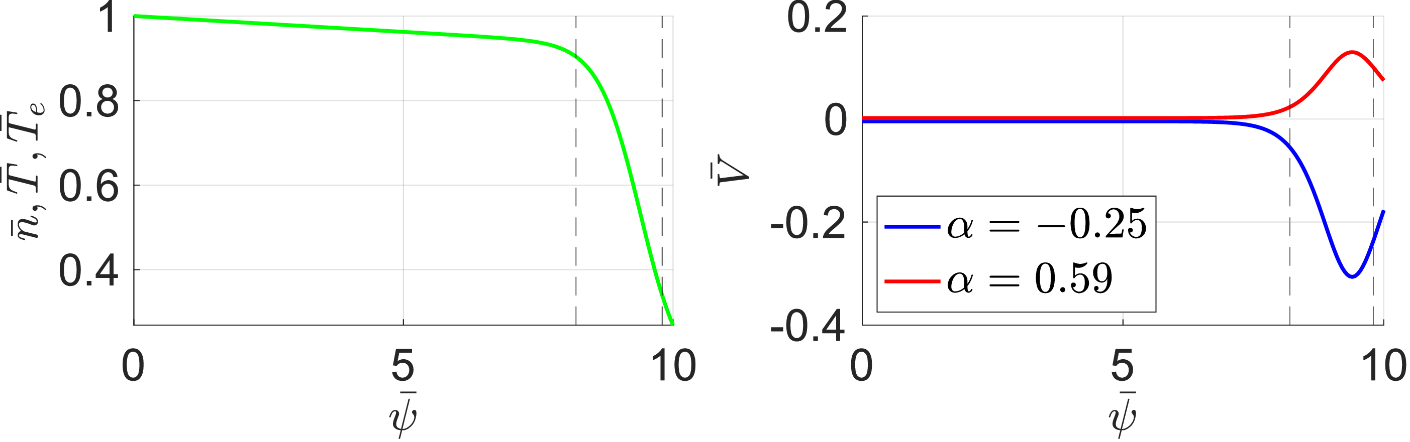
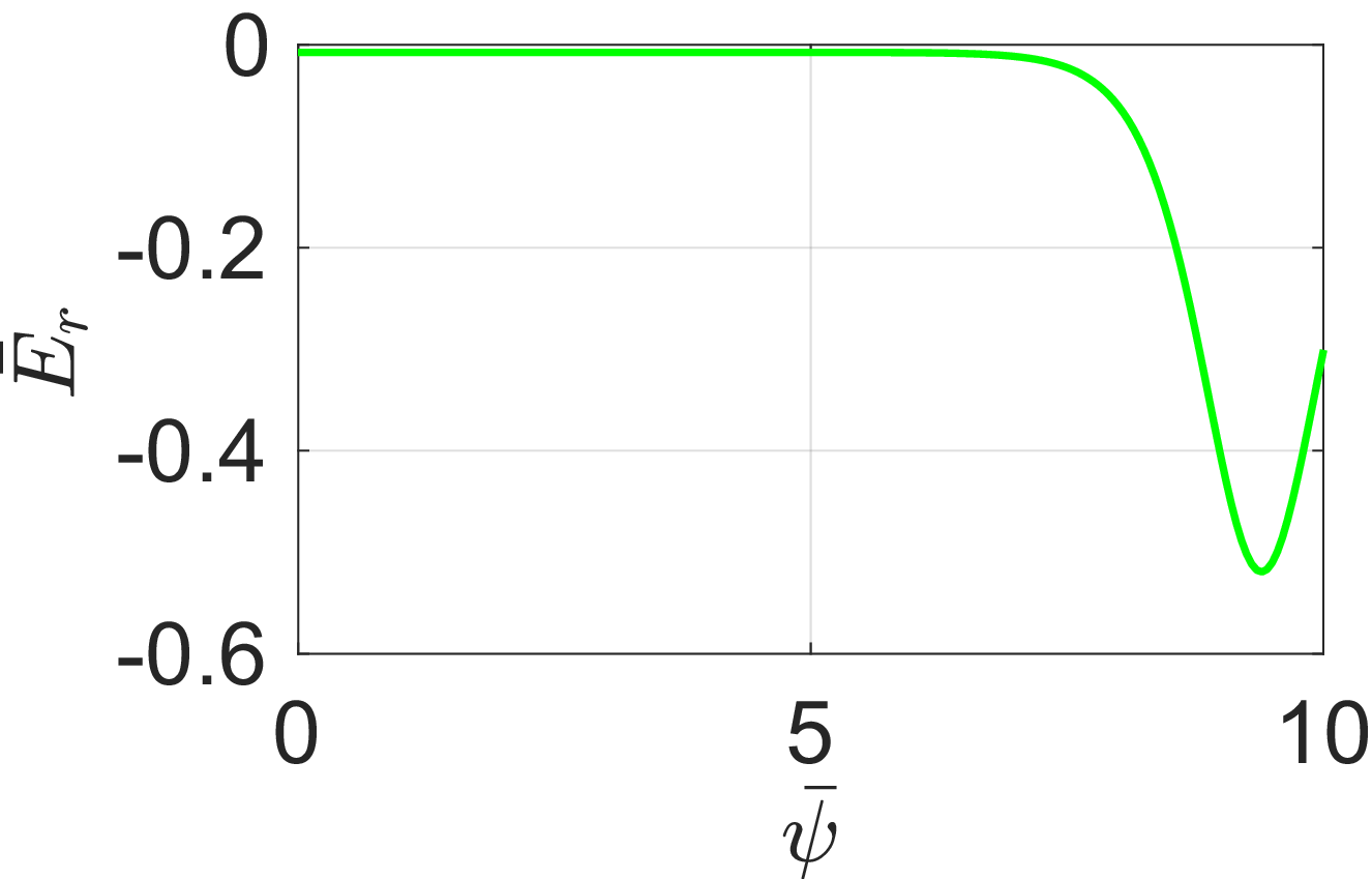
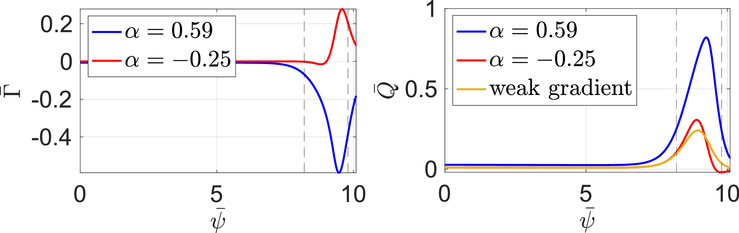
 α=−0.25
 α=0.59
 ϕ¯θ=ϕ¯ccosθ+ϕ¯ssinθ
 α=0.59
 α=−0.25
 ϕ¯c
ϕ¯c ϕ¯s
ϕ¯s ψ¯
ψ¯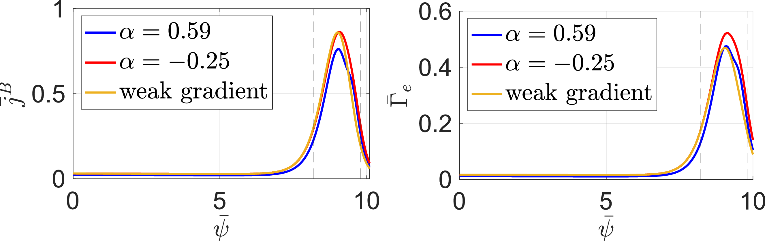
 α=−0.25
 α=0.59
 α=0.59
 α=−0.25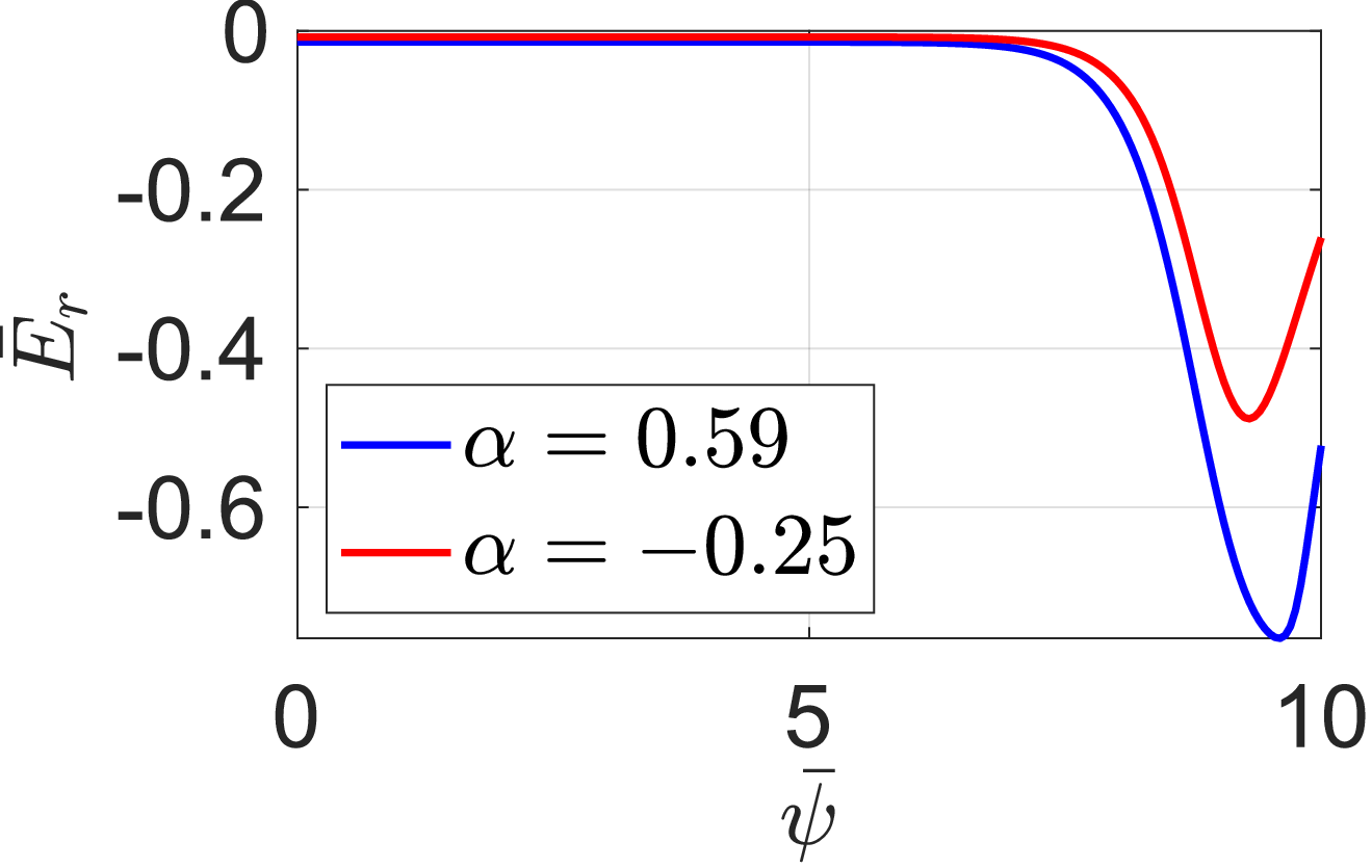
 α=0.59
 α=−0.25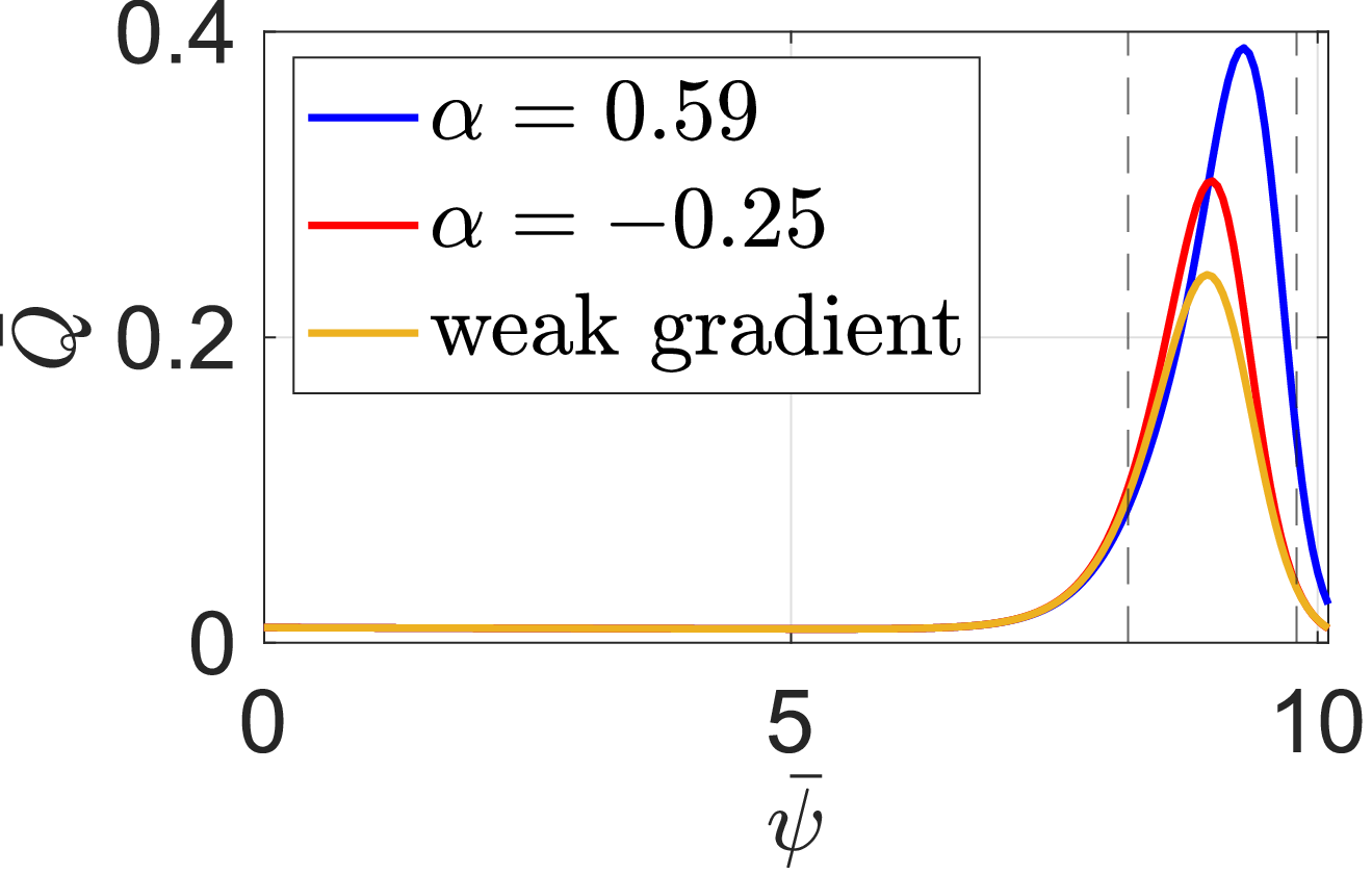
 α=0.59
 α=−0.25
 ϕ¯θ=ϕ¯ccosθ+ϕ¯ssinθ
 α=0.59
 ϕ¯c
ϕ¯c ϕ¯s
ϕ¯s ψ¯
ψ¯ α=−0.25
 ϕ¯s
ϕ¯s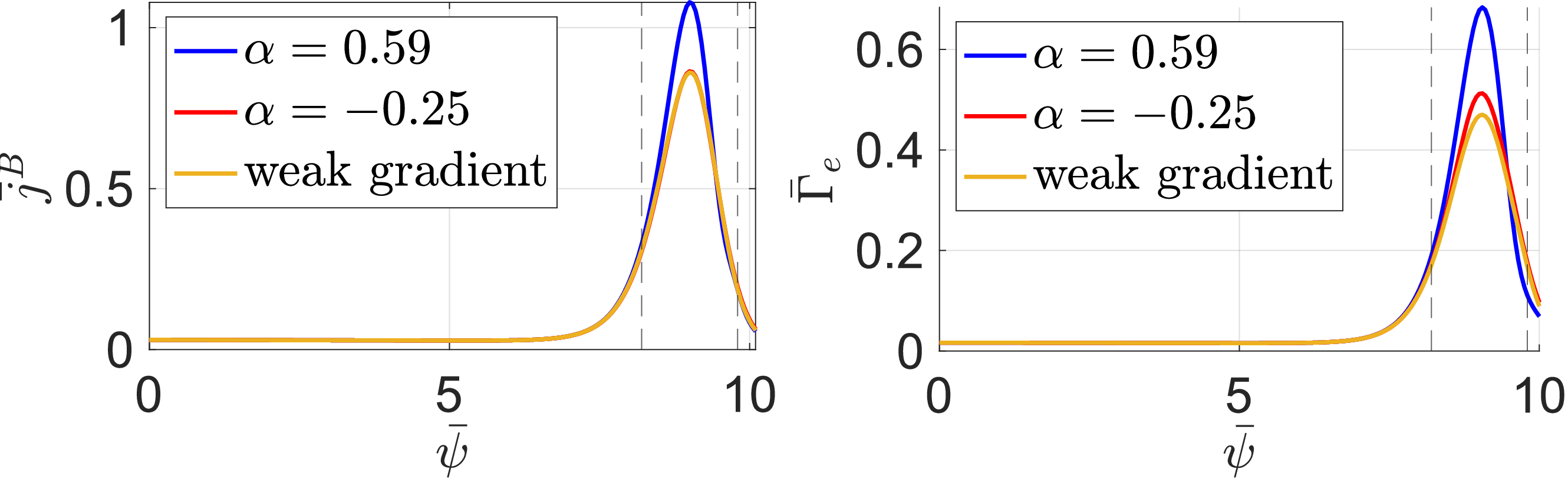
 α=0.59
 α=−0.25
 α=0.59
 Open access

