







1. Introduction
Methods to modify and control the boundary layer behaviour have been sought from the earliest stage of boundary layer studies and, in this respect, wall-normal transpiration immediately appeared as a relatively simple and very effective control technique. Already in Prandtl's very first paper on boundary layer theory, he showed the possibility of avoiding flow separation on one side of a circular cylinder with the application of a small amount of suction through a spanwise slit on the surface (see Prandtl Reference Prandtl1904). Localized suction has also been explored as a technique to postpone separation on wings and hence to increase the maximum lift coefficient (Schrenk Reference Schrenk1935; Poppleton Reference Poppleton1951). Furthermore, since wall suction has a strong stabilizing effect on boundary layers, it has been investigated as a technique to delay the laminar–turbulent transition to accomplish drag reduction by the inherent lower friction drag of a laminar boundary layer in comparison with a turbulent boundary layer (TBL) (see Ulrich (Reference Ulrich1947) and Kay (Reference Kay1948) among others). Distributed blowing has been investigated as a skin-friction drag reduction technique for TBLs (see Kornilov (Reference Kornilov2015) for a review on the topic), while localized blowing, known as film cooling, is commonly adopted for the thermal protection of surfaces exposed to high-temperature flows such as the turbine blades of jet engines (see e.g. Goldstein Reference Goldstein1971).
Despite the practical interests of boundary layers with wall-normal mass transfer and the numerous investigations on the topic, fundamental understanding of the phenomena occurring in TBLs in the presence of wall transpiration is limited. Considerable disagreement persists in the literature even on the description of basic quantities, such as the mean streamwise velocity, for the rather simplified case of flat-plate boundary layer flow with uniform transpiration and no pressure gradient.
The case of a zero pressure gradient (ZPG) boundary layer with uniform suction applied at the wall is of particular interest because it is possible to achieve a state for which the momentum loss due to wall friction is exactly compensated by the entrainment of high-momentum fluid due to suction, hence the boundary layer thickness remains constant in the streamwise direction. For the laminar regime the condition  $\partial /\partial x = 0$, where $x$ is the streamwise coordinate, leads to an analytical solution of the Navier–Stokes equation and the mean-velocity profile is represented by the equation
 \begin{equation} \frac{U}{U_\infty}=1-e^{yV_0/\nu}, \end{equation}
where  $U$ is the streamwise velocity, $U_\infty$ the free stream velocity, $y$ the wall-normal coordinate, $V_0<0$ the suction velocity and $\nu$ the kinematic viscosity of the fluid. This streamwise-invariant state is known as the asymptotic suction boundary layer (ASBL) and the exponential profile of (1.1) was originally derived analytically by Griffith & Meredith (Reference Griffith and Meredith1936), experimentally verified by Kay (Reference Kay1948) and later by Fransson & Alfredsson (Reference Fransson and Alfredsson2003) over a streamwise distance of more than $400\delta _{99}$ (where $\delta _{99}$ is the 99 % boundary layer thickness).
It is natural to hypothesize that an analogous asymptotic state exists also for TBLs, as indicated in the sketch of figure 1. However, a turbulent asymptotic suction boundary layer (TASBL) appears to be considerably more difficult to obtain than its laminar counterpart. While Kay (Reference Kay1948) conjectured that ‘an asymptotic turbulent suction profile may be closely approached at sufficient values of suction velocity’, Dutton (Reference Dutton1958) concluded that a spatially invariant TBL can be established just for a specific suction rate (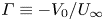 $\varGamma \equiv -V_0 / U_\infty$). Black & Sarnecki (Reference Black and Sarnecki1958) proposed instead that for every suction rate there is an asymptotic value of the momentum thickness Reynolds number $Re_\theta = f(\varGamma )$: this state is reached rapidly when the asymptotic momentum thickness is close to the one at the beginning of the suction, otherwise a large development length is required to reach the asymptotic condition. The slow approach to the asymptotic state was also reported by Tennekes (Reference Tennekes1964, Reference Tennekes1965), who, furthermore, suggested that a minimum suction rate is necessary for obtaining the asymptotic state ( $-V_0^+ \gtrsim 0.04$). More recently, Bobke, Örlü & Schlatter (Reference Bobke, Örlü and Schlatter2016) numerically obtained two TASBLs through large eddy simulations (LES) and raised doubts on the possibility of obtaining an ASBL in a practically realizable experiment due to the very long streamwise suction length required, claiming that ‘a truly TASBL is practically impossible to realise in a wind tunnel’. Moreover, it has been known from the earliest experiments on suction boundary layers (Black & Sarnecki Reference Black and Sarnecki1958; Dutton Reference Dutton1958; Tennekes Reference Tennekes1965) that at a high enough suction rate an initially TBL would eventually relaminarize, hence the asymptotic state obtained for $x \rightarrow \infty$ would, in that case, be the laminar ASBL. There are, however, considerable differences in the reported values for the threshold suction rate $\varGamma _{sst}$ below which a self-sustained turbulent state is observed. While Dutton (Reference Dutton1958) and Tennekes (Reference Tennekes1964) suggested $\varGamma _{sst}\approx 0.01$, Watts (Reference Watts1972) proposed the lower value of $\varGamma _{sst}=0.0036$, which was closely confirmed in recent direct numerical simulations (DNS) by Khapko et al. (Reference Khapko, Schlatter, Duguet and Henningson2016), who reported $\varGamma _{sst}=0.00370$.
Turbulent boundary layer developing over a permeable flat plate with wall-normal suction (not to scale).

Different scalings of the mean velocity profile have been proposed for the TBL with suction, and a recent review on the topic can be found in Ferro (Reference Ferro2017). As with any other TBL flow, the turbulent suction boundary layer (TSBL) can be divided into a viscous sublayer where the viscous stresses are prevalent and a turbulent layer where the Reynolds stresses dominate. The asymptotic description of the viscous sublayer can be derived as (Rubesin Reference Rubesin1954; Mickley & Davis Reference Mickley and Davis1957; Black & Sarnecki Reference Black and Sarnecki1958)
 \begin{equation} U^+{=}\frac{1}{V_0^+}\left(e^{y^+V_0^+} -1\right), \end{equation}
where the superscript ‘ $+$’ indicates normalization in viscous units. For the turbulent layer, instead, two different scalings have been proposed. A bilogarithmic law, where the streamwise velocity is described by a series of logarithmic functions $a \ln ^2y +b \ln y +c$, has been derived from Prandtl's momentum-transfer theory by a number of authors (Rubesin Reference Rubesin1954; Clarke, Menkes & Libby Reference Clarke, Menkes and Libby1955; Mickley & Davis Reference Mickley and Davis1957; Black & Sarnecki Reference Black and Sarnecki1958; Stevenson Reference Stevenson1963; Rotta Reference Rotta1970; Simpson Reference Simpson1970) and more recently via analytical methods based on matched asymptotic expansions (Vigdorovich Reference Vigdorovich2004; Vigdorovich & Oberlack Reference Vigdorovich and Oberlack2008; Vigdorovich Reference Vigdorovich2016). The bilogarithmic law can be expressed in the form (Stevenson Reference Stevenson1963)
 \begin{equation} \frac{2}{V_0^+}\left(\sqrt{1+U^+V_0^+}-1\right)=\frac{1}{\kappa}\ln{y^+}+\mathcal{C}-\frac{2}{V_0^+}, \end{equation}
where the left-hand side is sometimes referred to as pseudo-velocity. Equation (1.3) reduces to the canonical logarithmic law of the wall as long as
 \begin{equation} \mathcal{C} \rightarrow B+\frac{2}{V_0^+}, \quad \mathrm{for}\ V_0^+ \rightarrow 0, \end{equation}
where  $B$ is the log-law intercept for the no-transpiration case. There is no consensus on the numerical values of the parameters $\kappa$ and $B$, which in general should be considered functions of the suction velocity. Nevertheless, a common choice among the supporters of the bilogarithmic scaling is to set $\kappa$ to the value of the non-transpired case.
Other authors (Kay Reference Kay1948; Dutton Reference Dutton1958; Tennekes Reference Tennekes1965; Andersen, Kays & Moffat Reference Andersen, Kays and Moffat1972; Bobke et al. Reference Bobke, Örlü and Schlatter2016) have instead proposed a logarithmic dependency of the streamwise velocity on the wall-normal coordinate, analogous to what is found for non-transpired boundary layers,
 \begin{equation} U^+ = A \ln y^+ + B, \end{equation}
with the slope  $A$ and the intercept $B$ of the line function of the suction rate. Among these studies, the approach by Tennekes (Reference Tennekes1965) is particularly original, where a law of the wall and a velocity defect law were derived for TSBLs in the modified set of variables ${V_0^+U^+ = f(y^+V_0^+)}$ and ${V_0^+(U^+-U_\infty ^+)=G(y/\delta )}$. Tennekes concluded that in the range ${0.04<-V_0^+<0.1}$, the logarithmic part of the profile shows the constant slope,
 \begin{equation} -V_0^{+} U^{+} \propto 0.06\ln{\left({-}y^+V_0^+\right)}. \end{equation}
For turbulent asymptotic boundary layers, though,  $-V_0^+U^+=U/U_\infty$, hence (1.6) can be rewritten in outer-scaling as
 \begin{equation} U/U_{\infty}\propto0.06\,\ln{\eta}, \end{equation}
where  $\eta$ is the wall-normal distance normalized with the boundary layer thickness $\delta$.
The available data on TSBLs appears to be insufficient to settle the controversy on the mean velocity scaling, moreover, experimental or numerical data on higher-order velocity statistics are rather scanty. For these reasons a larger database on turbulent suction boundary layer was judged to be necessary and a new experimental apparatus for wall-transpired boundary layers was built and brought into operation at the Linné Flow Centre at the Royal Institute of Technology in Stockholm (KTH). In the following sections, after descriptions of the experimental set-up and measurement procedures, the most significant experimental results will be reported, with the main focus on TASBLs.
2. Experimental set-up
The main component of the apparatus is a flat plate with a permeable top surface installed in the minimum turbulence level (MTL) wind tunnel in the Fluid Physics Laboratory at KTH. The maximum streamwise turbulence intensity for an empty test section is less than  $0.04\,\%$ in the speed range from $10\ \textrm {m}\ \textrm {s}^{-1}$ to $60\ \textrm {m}\ \textrm {s}^{-1}$ and a cooling system maintains the temperature of the flow constant with a maximum variation around the mean in space and time of ${\pm }0.07\,^\circ \textrm {C}$ (see Johansson (Reference Johansson1992) and Lindgren & Johansson (Reference Lindgren and Johansson2002) for a complete description of the wind tunnel). A drawing of the flat plate installed inside the wind-tunnel test section is shown in figure 2. The test section has a main two-dimensional (2-D) traverse in the $xy$-plane running on top of the roof with access through a centreline slot. To this traverse, there exist several spanwise traverses depending on the desired spanwise extent; however, to avoid probe vibrations using the main traverse at the relatively high speeds in the present study a landing traverse was specially designed, manufactured and brought in operation. This traverse lands on the plate using the main traverse and then moves the probe vertically by a third motor equipped with a rotary encoder ensuring a relative accuracy of the vertical displacement of the probe of ${\pm }1\ \mathrm {\mu }\textrm {m}$ (see figure 2 $c$). The extent of the upstream region influenced by the traverse system was checked moving the traverse system progressively closer to a fixed Prandtl tube and the deviation in velocity measured by the Prandtl tube was found to be less than $0.5\,\%$ from the undisturbed value. For further details about this traverse see Ferro (Reference Ferro2017). The flat plate is $6.6\ \textrm {m}$ long and spans the whole $1.2\ \textrm {m}$ width of the wind-tunnel test section. It starts with a $122\ \textrm {mm}$ long impermeable elliptical leading edge followed by eight individual plate elements, each one extending $812\ \textrm {mm}$ in the streamwise direction. Finally, a $1.2\ \textrm {m}$ long linear diffuser (not shown in figure 2) extends inside the wind-tunnel diffuser section from the plate trailing edge, expanding the flow to the full local cross-sectional area. The resulting streamwise extent of the suction area of the current apparatus is approximately 2.5 times larger than the largest apparatuses for the study of boundary layers with mass transfer known by the authors (Andersen et al. Reference Andersen, Kays and Moffat1972; Watts Reference Watts1972), with clear advantages for the study of the slow-evolving TSBLs.
Drawing of the experimental set-up mounted in the MTL wind-tunnel test section (dimensions in mm). The filled areas are the perforated surfaces; ( $a$) impermeable leading-edge section; ( $b$) leading-edge bleed slot; ( $c$) streamwise-moving traverse system ( $x$–
$x$– $y$); ( $d$) one of the six ceiling-height adjustment station; ( $e$) wall-mounted traverse system; ( $f$) oil-film measurement station. Note: the streamwise-moving traverse system was unmounted when performing oil-film or hot-wire measurements at the downstream station ( $e{,}f$).

The plate is installed in the test section such that the test surface constitutes the wind-tunnel bottom surface. Such an arrangement was preferred to the more common installation of the flat plate in the midheight of the test section for two reasons: firstly, the extra blockage originating from the suction/blowing tubing was deemed problematic; secondly, this configuration guarantees a longer vertical length of free stream, reducing possible confinement effects. In order to remove the boundary layer developed in the wind-tunnel contraction section and to allow the development of a fresh boundary layer with a well-defined origin on the test plate, the flow beneath the plate leading edge is vented through a bleed slot with an adjustable opening. A large ZPG region, with a maximum variation of free stream velocity of less than  ${\pm }0.5\,\%$ in the streamwise coordinate range $1.5\ \textrm {m} < x \lesssim 6.1\ \textrm {m}$, could be obtained for any experimental condition examined through iterative adjustment of the ceiling shape and regulation of the bleed-slot opening.
Each plate element is a sandwich construction. A  $0.9\ \textrm {mm}$ thick perforated titanium sheet is glued on a rectangular frame of L- and T-beams. All beams are perforated to ensure a uniform pressure in the plate inner chamber and are bolted on a $6\ \textrm {mm}$ thick bottom plate (see figure 3). The titanium sheets are laser drilled with $64\ \mathrm {\mu }\textrm {m}$ diameter holes with a centre-to-centre spacing of 0.75 mm in both spanwise and streamwise directions, giving a total open area of $0.56\,\%$. The holes are not aligned in the streamwise direction, instead, a random pattern with fixed centre-to-centre distance and fixed row spacing was chosen, in order not to introduce any preferential spanwise scale in the flow. Each plate carries a pressure tap facing the wind-tunnel test section, enabling the measurement of the streamwise pressure gradient. One of the plate elements is different from the others and, in addition to the pressure tap, it hosts a wall-mounted traverse system and a glass insert for oil-film interferometry skin-friction measurements. This plate was mounted in the most downstream position so that the wall-mounted traverse allows the measurement of boundary layer profiles in a location inaccessible to the main wind-tunnel traverse system. The wall-mounted traverse is equipped with a rotary encoder ensuring a relative accuracy of the vertical displacement of the probe of ${\pm }1\ \mathrm {\mu }\textrm {m}$. It has a range of $500\ \textrm {mm}$ and, hence, is able to move to the undisturbed free stream, where the hot-wire can be calibrated against a Prandtl tube. Whenever this measurement station was in use, the main wind-tunnel traverse system was unmounted in order to avoid the disturbances propagating downstream of it.
Exploded view of one plate element (dimensions in mm). The perforated titanium sheet (a) is supported by a hollow frame (b) mounted on the bottom plate (c). Below, three suction/blowing channels (e) from which air is driven to/from the fan. (d) Surface measurement access plug (pressure tap, hot-film probe or Preston tube). (f) Magnified photography of the laser-drilled titanium sheet.

For each plate section, 18 flexible hoses with an inner diameter of  $25\ \textrm {mm}$ depart from the side of the three suction channels on the bottom side of the plate. These flexible hoses are connected to eight manifolds (one for each plate) from which rigid steel pipes $125\ \textrm {mm}$ in diameter drive the flow to a suction chamber, where eight regulation valves allow the adjustment of the volume flow in each one of the steel pipes. This ensures that a uniform transpiration velocity can be obtained despite minor differences in the permeability of the titanium sheets. After regulation, the difference in wall-normal velocity between different plate elements could be kept within ${\pm }2.5\,\%$. The chamber is connected to a 7.5 kW AC centrifugal fan through a single pipe 200 mm in diameter equipped with a flowmeter measuring the total volume flow driven by the system with an extended uncertainty of ${\pm }1.5\,\%$. The regulation of the volume flow is obtained adjusting the fan rotation speed with a variable-frequency drive.
Velocity measurements were performed with constant-temperature hot-wire anemometry, using in-house boundary-layer-type single-wire probes with a wire length  $L_{w}$ ranging from $0.28\ \textrm {mm}$ to $0.6\ \textrm {mm}$ in combination with a Dantec StreamLine 90N10 frame and a 90C10 CTA module. Frequent in situ recalibration of the hot-wire probe against a Prandtl tube located in a constant temperature free stream flow allows the uncertainty of the velocity measurement to be kept within $1\,\%$. The experimental set-up and measurement procedures are described in greater detail in Ferro (Reference Ferro2017).
2.1. Verification of the experimental apparatus and measurement procedures
In order to verify the quality of the experimental apparatus and measurement procedures, several ZPG TBLs without transpiration and several laminar ASBLs were measured in the new set-up and compared with previous experimental and theoretical results. In the following,  $\delta ^\ast$, $\theta$ and $\delta _{99}$ denote the displacement, the momentum and the boundary layer thickness where the velocity has reached 99 % of $U_\infty$. The viscous length scale is denoted by $l^\ast$ and the Reynolds numbers $Re_\theta$ and $Re_\tau$ denote the momentum and friction Reynolds numbers, respectively.
The ZPG TBLs in absence of transpiration velocity were measured at different free stream velocities and different streamwise locations, including the most downstream measurement location, where the skin friction could be directly measured with oil-film interferometry. The skin-friction coefficient ( $C_{f}$) measured with oil-film interferometry at the most downstream measurement location is shown in figure 4. Good agreement between the measurements and the Coles–Fernholz skin-friction law
 \begin{equation} C_{f}=2\left(\frac{1}{\kappa}\ln Re_\theta + C\right)^{{-}2}, \end{equation}
with parameters,  $\kappa =0.384$ and $C=4.127$ as proposed by Nagib, Chauhan & Monkewitz (Reference Nagib, Chauhan and Monkewitz2007) is found, with larger deviation (even though limited to less than $2\,\%$) for the two smallest Reynolds numbers considered. For the seven boundary layer profiles measured at the most downstream measurement location ( $x=6.06\ \textrm {m}$), the friction velocity ( $u_\tau$) was obtained from the oil-film interferometry measurements. Table 1 lists the main experimental parameters for these boundary layers. The inner-scaled velocity profiles and the outer-scaled velocity-defect profiles, with the Rotta–Clauser length scale $\varDelta =\delta ^*U_\infty /u_\tau$ as the outer length scale, are shown in figures 5 and 6, respectively, together with the linear and logarithmic law of the wall,
 \begin{equation} U^{+} = \frac{1}{\kappa} \ln y^{+} + B, \end{equation}
with  $\kappa =0.384$ and $B=4.173$ (Nagib et al. Reference Nagib, Chauhan and Monkewitz2007), and
 \begin{equation} U_\infty^{+} - U^{+} = -\frac{1}{\kappa}\ln \eta + B_1, \end{equation}
with  $\eta =y/\varDelta$, $\kappa =0.384$ and $B_1=-0.87$ (Monkewitz, Chauhan & Nagib Reference Monkewitz, Chauhan and Nagib2007).
Skin friction coefficient versus  $Re_\theta$ for all the profiles measured at the most downstream measurement station. The error bars show a ${\pm }2\,\%$ variation in $C_{f}$. Dashed line: Coles–Fernholz skin-friction law, (2.1) with coefficient $\kappa =0.384$ and $C=4.127$ (Nagib et al. Reference Nagib, Chauhan and Monkewitz2007).

Inner-scaled mean-velocity profiles for  $x=6.06\ \textrm {m}$. Dash-dotted line, linear-law; dashed line, log-law (2.2) with constants $\kappa = 0.384$ and $B=4.173$ (Nagib et al. Reference Nagib, Chauhan and Monkewitz2007).

Outer-scaled mean-velocity profiles for  $x=6.06\ \textrm {m}$. Dashed line: log-law (2.3) with constants $\kappa = 0.384$ and $B_1=-0.87$ (Monkewitz et al. Reference Monkewitz, Chauhan and Nagib2007).

Experimental parameters for the ZPG TBL profiles measured at  $x=6.06\ \textrm {m}$.

Since a direct measurement of the wall position with sufficient accuracy was unavailable, for the profiles shown in figures 5 and 6, the absolute wall position was obtained applying a wall-normal shift to the viscous scaled velocity profile, fitting it in a least square sense to DNS data in the inner region by Schlatter & Örlü (Reference Schlatter and Örlü2010) (corresponding to  $Re_\theta = 4060$). This procedure was only applied to experimental data points with $U^+<10$, corresponding to $y^+\lessapprox 13$. The shape factor $H_{12}$ for the non-transpired cases measured at all the measurement locations is shown in figure 7, and compared with the shape factor $H_{12,{num}}$ obtained from the integration of the composite velocity profile proposed in Chauhan et al. (Reference Chauhan, Monkewitz and Nagib2009). The majority of the measured profiles respect the shape-factor criteria $|H_{12} - H_{12,{num}}| < 0.008$ proposed by Chauhan et al. (Reference Chauhan, Monkewitz and Nagib2009) to determine whether a TBL can be considered canonical (in Chauhan et al. (Reference Chauhan, Monkewitz and Nagib2009) a different terminology is used, where equilibrium corresponds to what we here denote canonical), with more frequent deviations for $Re_\theta \lesssim 7500$. These deviations at lower Reynolds number can be an indication of over- or under-tripping or of history effects originating from the leading-edge pressure gradient. For large enough Reynolds number, however, the measured profiles can be considered to be canonical ZPG TBL profiles.
Shape factor  $H_{12}$ against the momentum thickness Reynolds number $Re_\theta$ for all the measured non-transpired cases. Filled symbols, profiles at $x=6.06\ \textrm {m}$; solid line, $H_{12,{num}}$ obtained from the integration of the composite profile proposed in Chauhan, Monkewitz & Nagib (Reference Chauhan, Monkewitz and Nagib2009); dashed line, $H_{12,{num}} \pm 0.008$; dotted line, $H_{12,{num}} \pm 1\,\%$.

The results on non-transpired TBLs illustrated above show that the measured boundary layers correspond well to the canonical ZPG TBL. Hence, it is possible to conclude that the experimental apparatus and experimental procedures are appropriate for an investigation on TBLs.
As additional verification, a series of suction boundary layer profiles were measured at the measurement location  $x=6.06\ \textrm {m}$. The suction was applied immediately downstream of the leading-edge section $x_{{s}} = 0.18\ \textrm {m}$ (in the following the subscript ‘ $s$’ will indicate the suction-start location) and no tripping tape was placed on the flat plate. In this configuration, the Falkner–Skan boundary layer developing on the leading-edge section is expected to evolve towards the ASBL velocity profile, which is obtained at a certain downstream distance on the plate. Several boundary layers at different suction rates and free stream velocities were measured and the intermittency factor of the velocity–time series was calculated with the user-independent method proposed by Fransson, Matsubara & Alfredsson (Reference Fransson, Matsubara and Alfredsson2005). The measured velocity profiles characterized by a fully laminar velocity profile are illustrated in figure 8 and compared with the analytical ASBL solution. In the figure, the displacement thickness Reynolds number of the ASBL solution $Re_{ASBL} = 1/\varGamma$ is also reported since it is the most commonly used parameter in the description of this flow. Excellent agreement is observed, proving that an ASBL was indeed obtained for all the suction rates $\varGamma \geq 3.38 \times 10^{-3}$, providing a second proof of the quality of the experimental apparatus and procedures, especially regarding the accuracy of the measured suction velocity. For the laminar ASBL profiles shown in figure 8, the absolute wall position was obtained applying a $y$-shift determined with a fit to the ASBL solution to the measured $y$. Since the fitting procedure acts as a rigid shift of the profile, it does not alter its shape, therefore the agreement observed in figure 8 between the experimental profiles and the ASBL solution cannot be considered an artefact of the fitting procedure.
Velocity profiles for fully laminar boundary layers at  $x=6.06\ \textrm {m}$. Solid line: ASBL analytical velocity profile (1.1).

3. Results and discussion
3.1. Self-sustained turbulence suction-rate threshold
Before discussing the turbulent state of the suction boundary layer, it is crucial to define the range of suction rate for which a turbulent state is self-sustained. It has been known since the earliest studies on suction boundary layers that an initially TBL will eventually relaminarize for large enough suction rates. However, there are considerable differences in the literature regarding the values of the threshold suction rate,  $\varGamma _{sst}$ (cf. references in § 1).
To obtain a measure of  $\varGamma _{sst}$, experiments were conducted in which suction was applied starting from the normalized streamwise location $Re_{x,{s}}$ downstream of an impermeable entry length on which a TBL developed (boundary layer tripping is applied on the leading- edge section). At a downstream distance $\Delta x$ from the commencement of suction, the velocity signal was measured in the inner region of the boundary layer ( $9\lesssim y^+ \lesssim 15$) and the intermittency factor ( $\gamma$), calculated with the user-independent method proposed by Fransson et al. (Reference Fransson, Matsubara and Alfredsson2005), was used to determine whether the signal is fully turbulent ( $\gamma = 1$), relaminarizing ( $0 < \gamma < 1$) or fully laminar ( $\gamma = 0$). The measurement was repeated for different values of $\varGamma$ and $Re_{x,{s}}$, and the results are shown in figure 9. We observe that for all the initial conditions and evolution lengths considered the measured self-sustained turbulence suction-rate threshold fall in a ${\pm }4\,\%$ bound from the value $\varGamma _{sst}=3.70\times 10^{-3}$ reported by Khapko et al. (Reference Khapko, Schlatter, Duguet and Henningson2016), close to the value of $\varGamma _{sst}=3.60\times 10^{-3}$ found by Watts (Reference Watts1972).
Intermittency factor  $\gamma$ of the near-wall velocity signal versus the suction rate $\varGamma$ for different suction-start locations $Re_{x,{s}}$ and streamwise evolution lengths $\Delta x/\delta _{99, {s}}$. Black solid line, $\varGamma _{{sst}} =3.70 \times 10^{-3}$ (Khapko et al. Reference Khapko, Schlatter, Duguet and Henningson2016); black dashed line, $\varGamma _{{sst}} =3.70 \times 10^{-3} \pm 4\,\%$; red dash-dotted line, $\varGamma _{{sst}} =3.6 \times 10^{-3}$ (Watts Reference Watts1972).

3.2. Development of TBL with suction
Turbulent suction boundary layers are expected to evolve towards an asymptotic condition for which the boundary layer becomes independent from the streamwise coordinate. Earlier works suggested that to experimentally obtain an asymptotic turbulent state is difficult (or even impossible (Bobke et al. Reference Bobke, Örlü and Schlatter2016)), mainly because the evolution towards the asymptotic state is slow, i.e. occurring over a streamwise distance many times larger than the initial boundary layer thickness. The evolution to the asymptotic state can, however, be hastened if the boundary layer thickness at the location of the suction start is chosen to be close to the asymptotic one (Black & Sarnecki Reference Black and Sarnecki1958; Dutton Reference Dutton1958; Tennekes Reference Tennekes1964). In order to test whether an asymptotic state could be obtained in the current set-up, a series of experiments were conducted in which the suction rate was kept constant while the streamwise Reynolds number of the suction-start location  $Re_{x,{s}}$ was gradually varied with a regulation of the free stream velocity and of the physical suction-start location. The latter regulation was obtained either disconnecting the upstream plate elements from the suction system or, when finer adjustment was needed, covering a portion of the surface with standard household aluminium foil. The results for different suction rates are shown in figure 10. In figure 10, $x' = x-x_{vo}$ represent the streamwise coordinate corrected for the virtual origin $x_{vo}$ calculated from the downstream development of the canonical ZPG TBL cases. For all the suction rates considered here, it was possible to experimentally obtain a boundary layer with approximately constant boundary layer thickness, moreover, for four out of five cases the same boundary layer momentum thickness Reynolds number could be obtained for different $Re_{x,{s}}$ (case $\blacktriangle$, red and $\blacklozenge$, yellow for $\varGamma \approx 3.27 \times 10^{-3}$; case $\blacktriangleright$, red and $\bullet$, green for $\varGamma \approx 3.07 \times 10^{-3}$; case $\bullet$, lightblue and ${\blacksquare }$, pink for $\varGamma \approx 2.65 \times 10^{-3}$; case $\blacktriangleleft$, green and
  , lightblue for $\varGamma \approx 2.56 \times 10^{-3}$), suggesting that the turbulent asymptotic state was indeed reached. For $\varGamma \approx 2.82 \times 10^{-3}$ no exact overlap of $Re_\theta$ is observed for different initial conditions, however, the downstream evolution of one measurement case (
 , pink) appears to be bounded between a case showing a slow decrease ( $\blacktriangleleft$, darkblue) and a case showing a slow increase ( $\blacktriangleright$, black) of the momentum thickness along the streamwise coordinate, thus suggesting that case (
 , pink) can be representative of the asymptotic state for this suction rate. In figure 11, the velocity mean and variance is compared for the boundary layer profiles measured at the most downstream measurement location obtainable by the main wind-tunnel traverse system ( $x = 4.80\ \textrm {m}$) for the subset of cases listed above. For these boundary layers, the wall shear stress was calculated using the von Kármán momentum integral equation modified for mass transfer. In the absence of pressure gradients and neglecting the streamwise variation of the Reynolds normal stresses difference, $\overline {u'^2} - \overline {v'^2}$, the following relation holds:
 \begin{equation} \left(\frac{u_\tau}{U_\infty}\right)^2=\frac{C_{f}}{2}=\frac{\mathrm{d} \theta}{\mathrm{d}x} - \frac{V_0}{U_\infty}. \end{equation}
The term  $\mathrm {d}\theta / \mathrm {d}x$ was determined from a fit of the measured momentum thicknesses to an exponential law of the type $Re_\theta = a Re_x^b$. Since the boundary layer profiles reported in figure 11 obey the inequality constraint $| \mathrm {d}\theta / \mathrm {d}x| < 0.02\,|{V_0}/{U_\infty }|$, it can be concluded that $C_{f}$ has the same uncertainty as to the suction rate, which was estimated to be ${\pm }2.5\,\%$. For all the TASBL profiles shown in the following figures, the absolute wall position was determined with a fit in the near-wall region ( $U^+<10.5$, corresponding to $y^+\lessapprox 18$) to the LES data by Bobke et al. (Reference Bobke, Örlü and Schlatter2016) for $\varGamma =3.00 \times 10^{-3}$. Despite that, the law of the wall for suction boundary layers is, in general, a function of both the absolute wall-normal position $y^+$ and the suction velocity $V_0^+$ in the range of suction rates considered (i.e. $2.5\times 10^{-3} < \varGamma < 3.70 \times 10^{-3}$), no significant difference is observed up to $y^+\approx 20$ and hence simulation data at a single suction rate can be used to fit all the measured TASBL profiles. An excellent agreement of the mean velocity profiles between the cases with matching suction rate is observed (see figure 11). The variance profiles for all the suction rates excluding $\varGamma = 2.82 \times 10^{-3}$ also show excellent agreement in the outer region of the boundary layer, while the observed deviation in the inner region can be explained by hot-wire spatial filtering effects. For $\varGamma = 2.82 \times 10^{-3}$ the velocity-variance profile shows small but observable differences in the outer region of the boundary layer, with the case (
 , pink) having variance values between the ones of the case ( $\blacktriangleright$, black) and of the case ( $\blacktriangleleft$, darkblue). It is concluded that all the cases reported in figure 11 excluding ( $\blacktriangleright$, black) and ( $\blacktriangleleft$, darkblue) can be considered turbulent asymptotic states. Figure 12 shows the mean velocity profiles at the three most downstream measurement locations for some of the cases identified as asymptotic. In the streamwise-coordinate interval considered, corresponding to a streamwise distance $\Delta x$ exceeding 20 times the boundary layer thickness $\delta _{99}$, the variation of momentum thickness is less than ${\pm }1.5\,\%$ for all the cases considered and the variation of the full mean-velocity profiles is minimal.
Momentum-thickness Reynolds number  $Re_\theta$ and shape factor $H_{12}$ evolution for different initial conditions at the suction-start location. Dashed lines, $Re_\theta =f(Re_{x'})$ (Nagib et al. Reference Nagib, Chauhan and Monkewitz2007); solid lines, power-law fit $Re_\theta =aRe_{x'}^b$.

Inner-scaled velocity mean and variance profiles at  $x=4.80\ \textrm {m}$. Dashed lines: viscous sublayer. Colours and symbols as in figure 10.

Inner-scaled mean-velocity profiles for some asymptotic cases at the three most downstream measurement locations. Here  $\Delta x$ represents the streamwise distance between the most upstream and the most downstream boundary layer profile shown in each graph. Colours as in figure 11. Dashed lines: viscous sublayer.

The variation with the suction rate of the asymptotic momentum-thickness Reynolds number and shape factor are shown in figures 13( $a$) and 13( $b$), respectively, and compared with the simulations results by Bobke et al. (Reference Bobke, Örlü and Schlatter2016) and Khapko et al. (Reference Khapko, Schlatter, Duguet and Henningson2016), showing a good agreement in the range of suction rates considered.
Asymptotic momentum thickness Reynolds number  $Re_{\theta,{\rm as}}$ and asymptotic shape factor $H_{12,{\rm as}}$ variation with the suction rate. Filled symbols, asymptotic cases in table 2; open blue squares, LES data by Bobke et al. (Reference Bobke, Örlü and Schlatter2016); open red diamonds, DNS data by Khapko et al. (Reference Khapko, Schlatter, Duguet and Henningson2016); vertical dashed lines, self-sustained turbulence threshold (Khapko et al. Reference Khapko, Schlatter, Duguet and Henningson2016).

Concluding, for all the suction rates considered it was possible to obtain a turbulent asymptotic state towards the downstream end of the flat plate: this was assessed observing that  $Re_\theta$ reached a constant value and that the mean velocity became invariant along the streamwise direction. For four out of the five suction rates considered, the asymptotic $Re_\theta$ and the asymptotic mean and variance velocity profile could be obtained with two different initial conditions at the suction-start location, which serves as an additional proof that the asymptotic state was indeed reached in a strict sense. For one suction rate ( $\varGamma \approx 2.82 \times 10^{-3}$) the asymptotic value of $Re_\theta$ and the velocity-variance profile could not be exactly reproduced with different initial conditions, however, $Re_\theta$ and the velocity-variance profile appear to be bounded by two measurement cases with respectively slightly higher and lower streamwise coordinate Reynolds number at the suction start $Re_{x,{s}}$.
3.3. Mean-velocity scaling for the turbulent asymptotic state
Figure 14 shows the viscous-scaled mean-velocity profile for some of the measured TASBLs. The profiles appear to be characterized by a large logarithmic region and by the absence of a clear wake region. The disappearance of the wake region was already reported in previous studies and appears to be such a fundamental characteristic of TASBLs that the presence of a wake region can be considered a characteristic of a boundary layer that has still not reached its asymptotic state (Black & Sarnecki Reference Black and Sarnecki1958; Simpson Reference Simpson1970; Bobke et al. Reference Bobke, Örlü and Schlatter2016). These observations suggest that the logarithmic law,
 \begin{equation} U^+{=}A(\varGamma) \ln y^+{+} B(\varGamma), \end{equation}
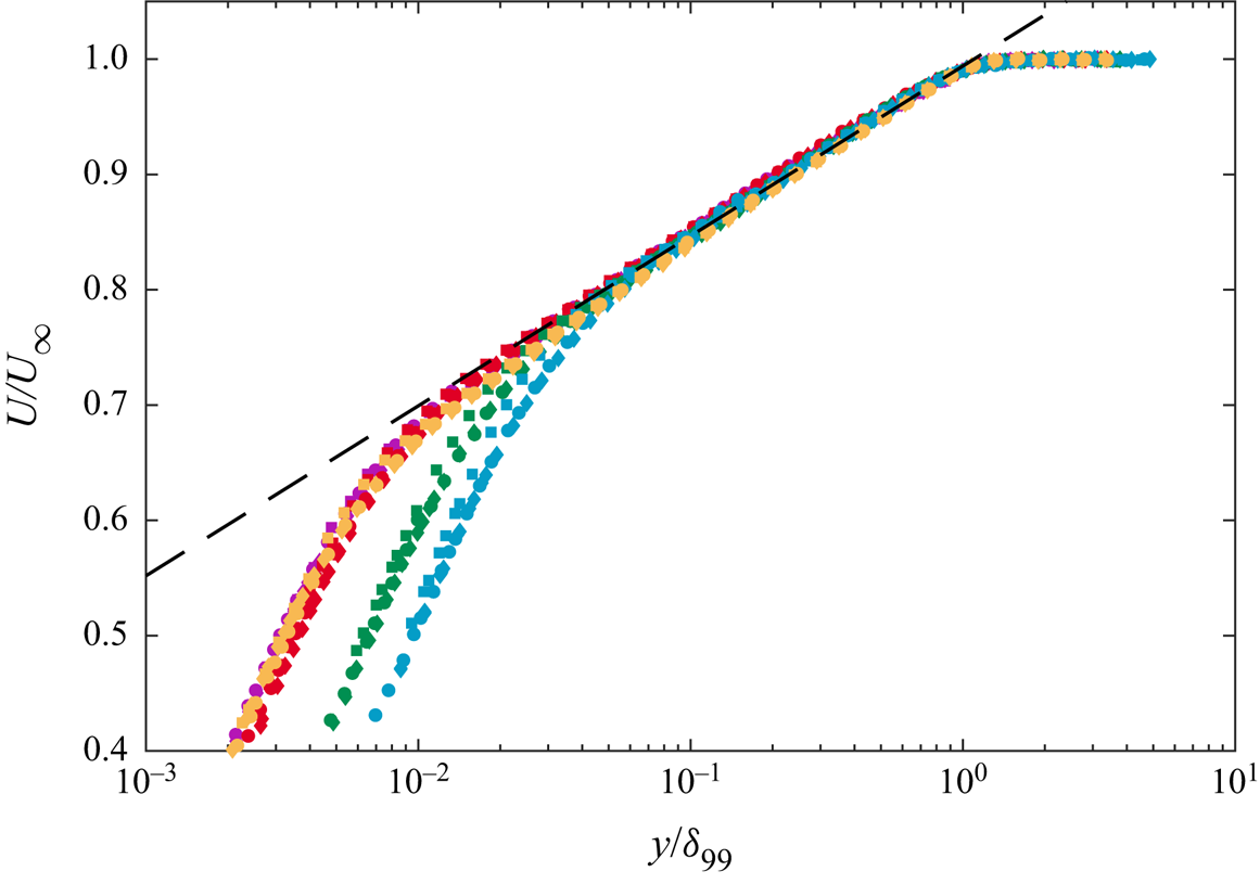
is a valid empirical description of the mean-velocity profile. However, a fairly large database of TASBLs at different suction rates is necessary to determine the functions  $A=f_1(\varGamma )$ and $B=f_2(\varGamma )$, while the amount of experimental or numerical data available is indeed limited. However, observing figure 15, depicting the mean-velocity profiles for the same boundary layers plotted in outer-scaling, a good overlap in the entire velocity defect region between all the TASBLs considered can be noticed, independent of the suction rate. It follows that, at least in the range of suction rate considered, the TASBLs profile can be described with the logarithmic law,
 \begin{equation} U/U_\infty=A_{o} \ln \eta + B_{o}, \end{equation}
with the slope  $A_{o}$ and the intercept $B_{o}$ being constants for a given suction rate. Three different choices ( $\delta _{99}$, $\delta ^*$ and $\theta$) of outer length scale are compared in figure 15, but no substantial difference between them can be observed.
Viscous-scaled mean-velocity profiles of some of the measured TASBLs at  $x=4.80\ \textrm {m}$. Dashed line: viscous sublayer for $\varGamma =2.80 \times 10^{-3}$. Symbols as in table 2.

Outer-scaled mean-velocity profiles of some of the measured TASBLs at  $x=4.80\ \textrm {m}$, for three different choices of the outer length scale. The multiplicative coefficients of the length scales were chosen solely for illustration purposes. Dashed line: (3.3) with $A_{o}=0.064$ and $B_{o}=0.994$. Symbols as in table 2.

To further verify the mean-velocity scaling proposed in (3.3), the indicator function,
 \begin{equation} \varXi=y\frac{\mathrm{d}(U/U_\infty)}{\mathrm{d}y}, \end{equation}
was calculated for all the TASBLs listed in table 2. Since the data were sampled non-equidistantly (namely with a logarithmic spacing) along the wall-normal coordinate, the derivative was calculated with a weighted central-difference scheme with the weights chosen following the procedure proposed by Fornberg (Reference Fornberg1998) in order to maximize the accuracy at the measurement locations. The results are illustrated in figures 16( $a$) and 16( $b$) in inner- and outer-scaled wall-normal coordinates, respectively. A clear plateau of the indicator function is observed for $y^+\gtrsim 150$ and $y/\delta _{99}\lesssim 0.5$ (corresponding to $y\approx \delta _{95}$), indicating that the mean-velocity profile shows a clear logarithmic behaviour along the wall-normal coordinate. The extent of this logarithmic region is particularly large, extending for more than $40\,\%$ of the boundary layer thickness already for the lowest Reynolds number (i.e. for the largest suction rate) considered ( $Re_\tau =1760$). The slope $A_{o}$ of the logarithmic region has been calculated for all the TASBLs profiles in table 2 as the mean value of the indicator function for $y^+>150$ and $y/\delta _{99}<0.5$ obtaining $A_{o}=0.064\pm 5\,\%$. With this choice for $A_{o}$, the intercept $B_{o}$ of the log-law can be calculated for each profile as the mean value for $y^+>150$ and $y/\delta _{99}<0.5$ of the function
 \begin{equation} \varPsi=U/U_\infty-A_{o}\ln \eta. \end{equation}
For the choice of outer-scale  $\eta = y/\delta _{99}$ and $A_{o}=0.064$, figures 16( $c$) and 16( $d$) illustrate the function $\varPsi$ in inner- and outer-scaled wall-normal coordinates, respectively. The averaged value of the intercept $B_{o}$ between all the profiles was found to be $B_{o}=0.994, 0.826 \ \mathrm {and}\ 0.815$ for $\eta =\delta _{99}, \delta ^* \ \mathrm {and}\ \theta$, respectively. The proposed mean-velocity scaling for TASBL is compared with previous numerical and experimental results in figure 17. The asymptotic profiles obtained numerically by Khapko et al. (Reference Khapko, Schlatter, Duguet and Henningson2016) and Bobke et al. (Reference Bobke, Örlü and Schlatter2016) appear to show outer-scaling similarity for all the suction rates considered, excluding the case $\varGamma =3.70\times 10^{-3}$ corresponding in Khapko et al. (Reference Khapko, Schlatter, Duguet and Henningson2016) to the maximum $\varGamma$ for self-sustained turbulence (i.e. $\varGamma _{{sst}}$). Moreover, the slope of the logarithmic region of mean-velocity profiles compares well with the one obtained in the current experiments (i.e. the dashed-line in figure 17). Good agreement on the slope of the logarithmic region is also found with the profile measured by Kay (Reference Kay1948) at the suction rate for which it was reported that a constant boundary layer thickness was obtained. However, the boundary layer thickness $Re_\tau$ (observable by the extent of $y/\delta _{99}$ in the logarithmic plot) appears small if compared with the simulation data or current experiments. The profile from Tennekes (Reference Tennekes1964), instead, deviates considerably from the one measured in the current experiments. This profile represents, however, a case where the boundary layer momentum thickness was still weakly growing and hence the asymptotic regime was not fully established.
Indicator function  $\varXi$ versus the inner-scaled (a) and outer-scaled (b) wall-normal coordinate and $\varPsi$ function for $A_{o}=0.064$ versus the inner-scaled (c) and outer-scaled (d) wall-normal coordinate for all the TASBls in table 2. Red dashed line, ${\varXi =0.064}$; red dash-dotted line, $\varPsi =0.0994$; grey dotted lines, limits of the logarithmic region ${y^+=150}$ and $y/\delta _{99}=0.5$.

Comparison between the proposed mean-velocity scaling and other experimental and numerical data. Black dashed line: log-law as in (3.3) with constants determined based on the present experimental data  $A_{o}=0.064$ and $B_{o}=0.994$; green, light blue, LES by Bobke et al. (Reference Bobke, Örlü and Schlatter2016); yellow, purple, dark blue, DNS by Khapko et al. (Reference Khapko, Schlatter, Duguet and Henningson2016); black hollow triangles, experiments by Tennekes (Reference Tennekes1964) (run 2-312; $x=878\ \textrm {mm}$); red hollow squares, experiments by Kay (Reference Kay1948).

Experimental parameters for all the measurement cases for which a TASBL was obtained and boundary layer parameters for the profile at  $x=4.80\ \textrm {m}$.

In order to verify the applicability of the bilogarithmic law (see (1.3)) on the results of the current experiments, the profiles of pseudo-velocity,
 \begin{equation} U_p \equiv \frac{2}{V_0^+}\left(\sqrt{V_0^+U^+{+}1} -1\right), \end{equation}
as defined by Stevenson (Reference Stevenson1963) are shown in figure 18. If a bilogarithmic law would describe the mean-velocity profiles of TASBLs, the pseudo-velocity profiles would exhibit an extended region where  $U_p \propto \ln y^+$. Moreover, Stevenson (Reference Stevenson1963) proposed that a log-law,
 \begin{equation} U_{p}=\frac{1}{\kappa}\ln y^{+} + B, \end{equation}
with  $\kappa$ and $B$ equal to the no-transpiration case (proposing the values $\kappa =0.419$ and $B=5.8$) represents the velocity profile independently of the suction or blowing velocity. In figure 18, (3.7) is shown for two different choices for the constants, the one proposed by Stevenson (Reference Stevenson1963) and the one adopted by Nagib et al. (Reference Nagib, Chauhan and Monkewitz2007) for the description of canonical ZPG TBLs. It is evident that with these choices of the constants, the bilogarithmic law in (3.7) does not describe the experimental data on ASBLs. Moreover, even though there is a region in which the profile of $U_{p}$ appears linear in a semilogarithmic plot, the extent of the logarithmic region of the pseudo-velocity profiles is considerably smaller than the one observed for the inner- or outer-scaled mean-velocity profiles (see figures 14 and 15). Thus, it can be concluded that a logarithmic law provides a better description of the mean-velocity profiles of the ASBLs than the bilogarithmic law.
Profile of pseudo-velocity  $U_p$ as defined by Stevenson (Reference Stevenson1963) for the same asymptotic profiles of figures 14 and 15. Dashed line: log-law (3.7) with $\kappa =0.419$ and $B=5.8$ as proposed in Stevenson (Reference Stevenson1963). Dash-dotted line: log-law (3.7) with $\kappa =0.384$ and $B=4.17$. Symbols as in table 2.

3.4. Profiles of streamwise velocity variance
The profiles of streamwise velocity variance for the TASBLs listed in table 2 are shown in figure 11. These measurements, however, suffer from insufficient spatial and temporal resolution of the hot-wire probe, with 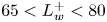 $65 < L_{w}^+ < 80$ and with values of $1/\,f_{max}^+$, where $f_{max}$ is the largest resolved frequency, exceeding the criterion $1/\,f_{max}^+ < 3$ proposed by Hutchins et al. (Reference Hutchins, Nickels, Marusic and Chong2009) for ensuring time-resolved measurements. In order to overcome these limitations and provide a better description of the streamwise velocity-variance profiles, a series of boundary layers was measured with the wall-mounted traverse system at $x=6.06\ \textrm {m}$, using hot-wire probes with smaller wire length and wire diameter, increasing hence both the spatial and temporal resolution. The experimental parameters for this set of experiments are listed in table 3. For each value of $\varGamma$ considered, the measurement has been repeated with three different hot-wire probes, in order to quantify and correct for the spatial filtering effects with the method proposed by Segalini et al. (Reference Segalini, Örlü, Schlatter, Alfredsson, Rüedi and Talamelli2011). This correction scheme relies on the dependence of the spatially averaged streamwise turbulence intensity on the wire length and on the spanwise correlation coefficient (Dryden et al. Reference Dryden, Schubauer, Mock and Skramstad1937), which in turn can be related to the local transverse Taylor microscale (Frenkiel Reference Frenkiel1949; Segalini et al. Reference Segalini, Örlü, Schlatter, Alfredsson, Rüedi and Talamelli2011): if the same flow field is measured with two or more hot-wire lengths, an estimate of the actual velocity variance can be obtained together with an estimate of the Taylor microscale. Even though other correction methods for hot-wire spatial filtering exist (Monkewitz, Duncan & Nagib Reference Monkewitz, Duncan and Nagib2010; Smits et al. Reference Smits, Monty, Hultmark, Bailey, Hutchins and Marusic2011), they were developed and calibrated for wall-bounded flow in the absence of wall transpiration and cannot hence be applied on TSBLs.
Experimental parameters for the suction cases at  $x=6.06\ \textrm {m}$.

When using the wall-mounted traverse system only one velocity profile at a fixed streamwise location can be obtained, hence the term  $\mathrm {d}\theta / \mathrm {d}x$ of the von Kármán momentum integral specialized for boundary layer with wall transpiration (see (3.1)) remains unknown. However, since the measurement cases considered in this section are similar in terms of suction rates and suction-start locations to those in § 3.2, for which $|\mathrm {d}\theta /\mathrm {d}x|<0.02\, |V_0/U_\infty |$ in the region $x>4.0\ \textrm {m}$, the additional systematic error on the wall shear stress introduced by neglecting the momentum-thickness derivative and assuming $C_f=-2V_0/U_\infty$ can hence be estimated to be less than $2\,\%$ in $C_f$, corresponding to less than $1\,\%$ in $u_\tau$. To assess whether the velocity profile measured is representative of asymptotic states, in figure 19 the mean-velocity profiles are compared with the log-law proposed in § 3.3 (see (3.3)). Good agreement with the proposed scaling is observed for all the profiles, with a somewhat larger deviation for the cases with $\varGamma \approx 2.56$ (yellow symbols), suggesting that the asymptotic state is just approximated but not fully obtained for this suction rate ( $\varGamma = 2.57 \times 10^{-3}$).


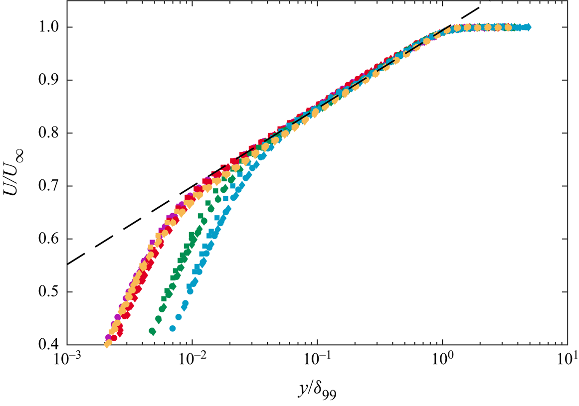
Figure 20 reports, for all the suction rates considered, the inner-scaled velocity-variance profiles corrected from spatial-filtering effects with the method by Segalini et al. (Reference Segalini, Örlü, Schlatter, Alfredsson, Rüedi and Talamelli2011), together with the measured profile at matched  $L_{w}^+ \approx 31$. Figure 20 also depicts a comparison with DNS and experimental corrected and uncorrected velocity-variance profiles for canonical ZPG TBLs. In the case of canonical ZPG TBLs, the measured streamwise velocity variance was corrected using the method proposed by Smits et al. (Reference Smits, Monty, Hultmark, Bailey, Hutchins and Marusic2011), since measurements of the same boundary layer with multiple hot-wire probes were not available. From figure 20 it appears that the velocity variance is strongly damped by the suction if compared with a canonical ZPG TBL, in agreement with previous studies (see e.g. Favre, Dumas & Verollet Reference Favre, Dumas and Verollet1961; Favre et al. Reference Favre, Dumas, Verollet and Coantic1966; Andersen et al. Reference Andersen, Kays and Moffat1972; Watts Reference Watts1972; Fulachier, Verollet & Dekeyser Reference Fulachier, Verollet and Dekeyser1977; Antonia et al. Reference Antonia, Fulachier, Krishnamoorthy, Benabid and Anselmet1988; Antonia, Spalart & Mariani Reference Antonia, Spalart and Mariani1994). For the suction rates investigated the reduction of the (corrected) near-wall peak ranges from approximately 50 %–65 % with respect to a canonical ZPG TBL with approximately the same $Re_\tau$. The magnitude of the near-wall peak of the inner-scaled velocity-variance profile is clearly dependent on the suction rate, with larger peak value for lower suction rates.
Inner-scaled velocity-variance profiles at  $x=6.06\ \textrm {m}$ for different suction rates compared with no-transpiration cases. Circles, TASBLs (measured data, $L_{w}^+\approx 31$); solid lines, TASBLs, corrected data (method Segalini et al. (Reference Segalini, Örlü, Schlatter, Alfredsson, Rüedi and Talamelli2011)); triangles, canonical ZPG TBL at $Re_\tau =5250$ (measured data, $L_{w}^+=19$); dash-dotted line, canonical ZPG TBL at $Re_\tau =5250$, corrected data (method Smits et al. (Reference Smits, Monty, Hultmark, Bailey, Hutchins and Marusic2011)); dashed line, canonical ZPG TBL at $Re_\tau =1145$, DNS by Schlatter & Örlü (Reference Schlatter and Örlü2010).

The variation of the velocity-variance peak with the suction rate is explicitly reported in figures 21( $a$) and 21( $b$) in inner- and outer-scaling, respectively, and compared with results of the numerical simulations by Bobke et al. (Reference Bobke, Örlü and Schlatter2016) (LES) and Khapko et al. (Reference Khapko, Schlatter, Duguet and Henningson2016) (DNS). An asymptotic suction state relation between the velocity variances scaled with inner and outer variables can readily be derived as
 \begin{equation} \overline{u'^2}^{+} = \frac{\overline{u'^2}}{-V_0 U_\infty} = \frac{\overline{u'^2}}{U_\infty^2}\frac{1}{\varGamma}, \end{equation}
which directly follows from (3.1) with the imposed condition of  $\mathrm {d}\theta / \mathrm {d}x = 0$ to guarantee the asymptotic state. Noteworthy is that this relation, valid in the asymptotic suction limit, only holds for $\varGamma \lesssim \varGamma _{{sst}}$, while in the limit of $\varGamma \rightarrow 0$ the asymptotic suction state will never be reached and, hence, (3.8) will not hold.
Maximum of the velocity variance in inner (a) and outer (b) scaling. Open circles, current experiments, measured data for  $L_{w}^+\approx 31$; filled circles, current experiments, corrected data (method by Segalini et al. (Reference Segalini, Örlü, Schlatter, Alfredsson, Rüedi and Talamelli2011)); blue squares, LES by Bobke et al. (Reference Bobke, Örlü and Schlatter2016); red diamonds, DNS by Khapko et al. (Reference Khapko, Schlatter, Duguet and Henningson2016); black dash-dotted line, (3.8) with $\overline {u'^2}_{peak}/U_\infty ^2 = 0.0108$; red dotted line, $\overline {u'^2}/U_\infty ^2=0.0108$; vertical dashed line, self-sustained turbulence threshold (Khapko et al. Reference Khapko, Schlatter, Duguet and Henningson2016).

Both the present experimental data and the LES (but not the DNS) seem to indicate that the velocity-variance peak scales with the outer velocity scale and, hence, to be independent of  $\varGamma$ (see figure 21 $b$). This is contrary to the mixed velocity scaling for the streamwise velocity fluctuations of ZPG TBLs first proposed by DeGraaff & Eaton (Reference DeGraaff and Eaton2000). The averaged experimental TASBL peak value corresponds to $\overline {u'^2}_{peak}/U_\infty ^2 = 0.0108$ (dotted line in figure 21 $b$) and can be used in (3.8) to obtain the variation of the velocity-variance peak in inner scaling as illustrated by the dash-dotted curve in figure 21( $a$). The behaviour is consistent with ZPG TBL results in the sense that the velocity-variance peak in inner scaling increases with $Re_\tau$ (see e.g. Marusic, Mathis & Hutchins Reference Marusic, Mathis and Hutchins2010), or as here with decreasing $\varGamma$. From figure 21 it is clear that the behaviour of the DNS data is different with respect to the experimental data and the LES. The reason for the difference between our experiments and the DNS at similar $\varGamma$-values is unknown but this data is taken relatively close to $\varGamma = \varGamma _{{sst}}$ and could potentially give rise to underdeveloped TASBLs.
From figure 20 we observe that the streamwise velocity-variance profiles decrease monotonically from the inner-peak location to the zero value at the boundary layer edge. For non-transpired canonical boundary layers (canonical ZPG TBL, turbulent pipe flow and turbulent channel flow) a shoulder in the outer part of the inner-scaled velocity-variance profiles is present which becomes more evident with increasing Reynolds number, taking the shape of a plateau for high enough Reynolds numbers. (Whether or not an outer peak of the streamwise-velocity variance appears at high enough Reynolds number is a matter of debate, see e.g. Hutchins et al. (Reference Hutchins, Nickels, Marusic and Chong2009), Vallikivi, Hultmark & Smits (Reference Vallikivi, Hultmark and Smits2015) and Monkewitz & Nagib (Reference Monkewitz and Nagib2015).) It has been shown (Marusic et al. Reference Marusic, Mathis and Hutchins2010; Ng et al. Reference Ng, Monty, Hutchins, Chong and Marusic2011) that this increase with Reynolds number of the magnitude of the velocity-variance profiles in the outer region can be attributed to the large and very large-scale motions. Based on the present data, it can hence be speculated that even small values of wall suction, such as those applied in this experiment, are very effective in reducing the strength of the larger scales of a TBL.
The outer region of the velocity-variance profiles also deserves some attention. In figure 22 the inner- and outer-scaled velocity-variance profiles are plotted versus the outer-scaled wall-normal distance for the current experiments and the simulations data by Bobke et al. (Reference Bobke, Örlü and Schlatter2016) and Khapko et al. (Reference Khapko, Schlatter, Duguet and Henningson2016). The experimental data show larger scatter if inner-scaling is adopted, while the opposite is observed for the simulation data, for which a good scaling of  $\overline {u'^2}^+$ occurs in the region ( $y/\delta _{99}>0.4$) for all the suction rates excluding the lowest ( $\varGamma =2.50\times 10^{-3}$). The reason of this discrepancy between experiments and simulations is at the moment unclear, even though it can be hypothesized that analogous to what happens in pipe flow (Doherty et al. Reference Doherty, Ngan, Monty and Chong2007), the achievement of a fully developed (asymptotic) turbulent state for the velocity-variance profile requires a longer streamwise distance than for the mean-velocity profile.
Outer- (a) and inner- (b) scaled velocity-variance profiles. Current experiments (symbols) and available numerical simulations (green, light blue, Bobke et al. (Reference Bobke, Örlü and Schlatter2016); yellow, purple, dark blue, Khapko et al. (Reference Khapko, Schlatter, Duguet and Henningson2016)) (solid lines) in both (a) and (b).

For TASBLs, however, a relationship between the inner-scaled Reynolds shear stress and the outer-scaled mean velocity profile can be established from which it is possible to derive the expected scaling of the velocity-variance profile. For TASBLs the following relation holds:
 \begin{equation} V_0\frac{\partial U}{\partial y}=\frac{1}{\rho}\frac{\partial \tau}{\partial y}, \end{equation}
where  $\tau =\mu \partial U/ \partial y - \rho \overline {u'v'}$ is the total shear stress. Equation (3.9) can readily be derived from the 2-D Reynolds-averaged Navier–Stokes equations imposing the asymptotic conditions $\partial /\partial x=0$. Integrating (3.9) from the wall to an arbitrary wall-normal position and recalling that for an ASBL $\tau _w = -\rho U_\infty V_0$, one obtains
 \begin{equation} \frac{\tau}{\tau_w}=1-\frac{U}{U_\infty}. \end{equation}
For a TBL  $\tau \approx -\rho \overline {u'v'}$ everywhere except in the near-wall region, hence, for the large outer portion of the boundary layer,
 \begin{equation} -\frac{\overline{u'v'}}{u_\tau^2}\approx1-\frac{U}{U_\infty}, \end{equation}
relating the inner-scaled Reynolds shear stress to the outer-scaled mean velocity profile. A similarity between the outer-scaled streamwise mean velocity profile of TASBL at different suction rates, as proposed in § 3.3, hence implies a similarity between the viscous scaled Reynolds stress  $\overline {-u'v'}^+$ (and vice versa), giving
 \begin{equation} \frac{U}{U_\infty} = f_1(\eta) \iff \overline{-u'v'}^{+} = 1-f_1(\eta) . \end{equation}
Furthermore, as the various components of the Reynolds stress tensor should have the same scaling if similarity is observed, the proposed similarity of the mean-velocity profile in outer-scaled variables leads to  $\overline {u'^2}^+ = f(\eta )$, just as the simulation results by Bobke et al. (Reference Bobke, Örlü and Schlatter2016) and Khapko et al. (Reference Khapko, Schlatter, Duguet and Henningson2016) are showing.
Given the small amount of experimental and numerical data on TASBLs, a firm conclusion on the scaling of the velocity variance in TASBLs should wait for data covering a larger range of suction rates (and hence  $Re_\tau$) from more independent sources. However, if a Reynolds number similarity of the Reynolds stress tensor is confirmed for TASBLs, it would constitute a solid ground to explain the observed outer-scaling of the mean-velocity profile, as apparent from the expression (3.12), derived from the Navier–Stokes equations for a 2-D TASBL with the only assumption being negligible viscous stress.
3.5. Spectra
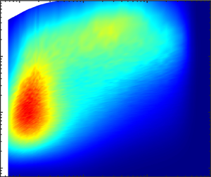
To conclude this description of TASBLs, figure 23 depicts the inner-scaled premultiplied power spectral density (PSD) map for all the suction cases at  $x=6.06\ \textrm {m}$ obtained with matching $L_{w}^+ \approx 31$. The PSD were estimated from the streamwise-velocity time series using Welch's method (Welch Reference Welch1967). The wavelengths were inferred from the time series of velocity using Taylor's hypothesis of ‘frozen turbulence’ (Taylor Reference Taylor1938) and the local mean velocity as the convective velocity of the waves.
Premultiplied PSD maps in inner-scaling for the suction cases measured at  $x=6.06 \ \textrm {m}$ with matching $L_{w}^+$ ( $\approx 31$).

As conjectured from the analysis of the velocity-variance profiles, suction is very effective in reducing the strength of the large scale structures present in TBLs, so that TASBLs (at least at the suction rates considered) appear to be fundamentally dominated by the near-wall cycle. This is particularly evident if the power-spectra maps of the two lowest suction cases are compared with a canonical ZPG TBL at comparable  $Re_\tau$ (figure 24), for which a clear contribution of the large energy components is observed in a large portion of the boundary layer.
Premultiplied PSD maps in inner-scaling for the ZPG TBL case measured at  $x=6.06\ \textrm {m}$ with $Re_\tau = 5250$ and $L_{w}^+ \approx 19$.

The streamwise wavelength  $\lambda ^+_{x,{p}}$ related to the peak of the premultiplied PSD increases with the suction rates, as clearly illustrated in figure 25. For the non-transpired case the peak in $f^+P_{uu}^+$ occurs at $\lambda ^+_{x,{p}}\approx 1000$ (in agreement with Jiménez, Del Álamo & Flores (Reference Jiménez, Del álamo and Flores2004) and Hutchins & Marusic (Reference Hutchins and Marusic2007) among others), while for suction this peak-length scale increases gradually with suction and reaches $\lambda ^+_{x,{p}}\approx 2700$ for $\varGamma = 3.70 \times 10^{-3}$. Since the peak in the premultiplied PSD corresponds to the signature of near-wall motion of the high- and low-speed streaks firstly observed by Kline et al. (Reference Kline, Reynolds, Schraub and Runstadler1967), the increase of the $\lambda ^+_{x,{p}}$ with the suction rate is in qualitative agreement with the measurements and flow visualization of a (localized) suction boundary layer by Antonia et al. (Reference Antonia, Fulachier, Krishnamoorthy, Benabid and Anselmet1988), who reported that ‘low-speed streaks tend to oscillate less in a spanwise direction while their streamwise persistence is increased (compared with the non-transpired case)’. Since the instability of the near-wall streaks plays a major role in the production of turbulence (see Kim, Kline & Reynolds (Reference Kim, Kline and Reynolds1971) and Jiménez & Pinelli (Reference Jiménez and Pinelli1999) among others), the increased stability of the near-wall streaks can be related to the decrease of the Reynolds stresses in presence of wall-normal suction, as proposed by Antonia et al. (Reference Antonia, Fulachier, Krishnamoorthy, Benabid and Anselmet1988).
Premultiplied PSD maps in inner-scaling for  $y^+ \approx 15$ at $x=6.06\ \textrm {m}$. Coloured lines, suction cases with $L_{w}^+ \approx 31$; black line, canonical ZPG TBL with $Re_\tau = 5250$ and $L_{w}^+ \approx 19$.

4. Conclusions
A new experimental set-up to investigate the existence of turbulent TASBL has been designed, manufactured and validated. Experimental turbulent suction boundary layers are proved to exist for suction rates  $\varGamma < 3.7 \times 10^{-3}$ in accordance with Watts (Reference Watts1972) and Khapko et al. (Reference Khapko, Schlatter, Duguet and Henningson2016): for larger suction rates an initially TBL undergoes a process of relaminarization. Turbulent asymptotic states can be established experimentally with the present set-up for the range of suction rate $2.55 \times 10^{-3} < \varGamma < 3.7 \times 10^{-3}$.
The mean-velocity profiles of TASBLs are characterized by the disappearance of the wake region and by a logarithmic behaviour for a particularly large portion of the boundary layer (covering 40 % of the boundary layer thickness already at  $Re_\tau = 1760$). A good overlap of the mean velocity profile in outer-scaling ( $U/U_\infty$ versus $\eta$) independently from the suction rate is observed and a log-law with slope $A_{o} = 0.064$ and intercept $B_{o} = 0.994$ (if $\eta = y/\delta _{99}$) describes accurately the outer-scaled mean-velocity profiles. A possible explanation of the observed mean-velocity scaling is proposed: if the shear stress scales with the wall-shear stress independently of the Reynolds number (or equivalently, of the suction rate), as observed in parallel turbulent shear flows (pipe flow and channel flow), the scaling of the mean velocity with the free stream velocity follows from (3.10), derived from the Navier–Stokes equation for a TASBL.
The application of suction leads to strong damping of the velocity fluctuations, with a large decrease of the magnitude of the near-wall peak of the streamwise-velocity variance, characterized by values from  $50\,\%$ to $65\,\%$ lower than canonical ZPG TBLs at comparable $Re_\tau$. The damping of the velocity fluctuations by suction appears to be primarily due to the increased stability of the near-wall streaks (in agreement with Antonia et al. (Reference Antonia, Fulachier, Krishnamoorthy, Benabid and Anselmet1988)), as can be concluded from the increase with the suction of the streamwise wavelength $\lambda ^+_{x,{p}}$ related to the peak of the premultiplied PSD in the near-wall region. The analysis of the PSD maps and the disappearance of the shoulder in the streamwise-velocity variance profile suggests that suction is very effective in reducing the strength of the (outer) large-scale structures of the boundary layer. Hence, TASBLs appear to be fundamentally dominated by the near-wall cycle. Future experiments should address the near-wall streaks through two-point cross-correlation measurements.
Declaration of interests
The authors report no conflict of interest.




 Open access

