







1. Introduction
Rayleigh–Darcy convection is observed in fluid-saturated porous media heated from the bottom and cooled from the top (Horton & Rogers Reference Horton and Rogers1945; Lapwood Reference Lapwood1948; Graham & Steen Reference Graham and Steen1994). The fluid in contact with the heated bottom boundary becomes warmer, and thus lighter, than the fluid located above it. This creates an intrinsically unstable vertical density stratification, with dense fluid lying on top of light fluid: a fluid parcel that, under the action of a small perturbation is displaced vertically upwards compared with its initial equilibrium position, will be surrounded by denser fluid, and will consequently experience a buoyancy force that will tend to push it further away from the initial position. At the same time, cold and dense fluid is dragged downwards, and convection can start. However, bottom-up heating does not always give convection: when the supplied heating flux is not large enough, diffusion (of momentum and heat) is able to dissipate the injected energy and to keep the flow quiescent, despite the presence of an unstable density stratification. The single parameter that characterizes the above-mentioned dynamics is the Rayleigh–Darcy number  $Ra$ – the ratio of buoyancy to dissipative forces. When $Ra$ is small, dissipative forces are large enough to balance the destabilizing effect of buoyancy, and the fluid does not move. When $Ra$ increases and exceeds a certain threshold, dissipative forces can no longer counteract buoyancy, and convection sets in. When convection takes place, it can largely increase the amount of vertical heat flux that can be transferred across the porous layer. This is usually quantified in terms of the Nusselt number $Nu$ – the ratio of convective to diffusive heat flux.
In recent years, Rayleigh–Darcy convection has received a lot of attention because of its relevance in the process of carbon dioxide (CO $_2$) sequestration in geological reservoirs (Hidalgo et al. Reference Hidalgo, Fe, Cueto-Felgueroso and Juanes2012; Huppert & Neufeld Reference Huppert and Neufeld2014; Riaz & Cinar Reference Riaz and Cinar2014; Emami-Meybodi et al. Reference Emami-Meybodi, Hassanzadeh, Green and Ennis-King2015; De Paoli Reference De Paoli2021). From a physical viewpoint, the process is as follows: upon injection into brine-filled geological formations, liquid CO $_2$ – which, when pure, is lighter than brine – dissolves in the brine (3 % in weight) and forms a heavier solute ( ${\rm CO}_2 + {\rm brine}$) that flows downward. Accurate evaluation of the flow field and of the associated transport flux is crucial to determine the optimal CO $_2$ injection rate into geological reservoirs, which typically feature $Ra$ up to ${\sim }{{O}}(10^5\unicode{x2013}10^6)$.
The current state of the art in the field is mostly based on two-dimensional computations (Graham & Steen Reference Graham and Steen1994; Otero et al. Reference Otero, Dontcheva, Johnston, Worthing, Kurganov, Petrova and Doering2004; Hewitt, Neufeld & Lister Reference Hewitt, Neufeld and Lister2012; Wen et al. Reference Wen, Chini, Dianati and Doering2013; Wen, Corson & Chini Reference Wen, Corson and Chini2015; De Paoli, Zonta & Soldati Reference De Paoli, Zonta and Soldati2016; Nield & Bejan Reference Nield and Bejan2017; Hewitt Reference Hewitt2020), focusing in particular on the flow stability and on the functional dependence between  $Ra$ – the forcing parameter of the flow – and $Nu$ – the response parameter. For $Ra<4{\rm \pi} ^2$, diffusion (dissipative forces) dominates and keeps the fluid quiescent, thus yielding $Nu=1$. At $Ra>4{\rm \pi} ^2$, buoyancy overtakes diffusion, and steady convection rolls spanning the full thickness of the porous layer appear, thus causing $Nu$ to increase. When $Ra\simeq 400$, the steady rolls are affected by the growth of boundary layer instabilities which, at $Ra \simeq 1300$, destabilize the organized roll pattern. Beyond this threshold, the flow enters the high- $Ra$ regime, which is characterized by chaotic formation of small plumes (protoplumes) within the boundary layer, and by their subsequent merging to form vertical megaplumes which stretch almost over the entire flow thickness. Reportedly, the scaling of $Nu$ with $Ra$ in this regime is nearly linear, $Nu \sim Ra$.
The dynamics of three-dimensional Rayleigh–Darcy convection remains relatively little explored. Most available numerical and experimental studies are limited to the low- $Ra$ regime, $Ra \sim {{O}} (1000)$ – and focus essentially on the stability of the flow and on the inception of convection (Elder Reference Elder1967; Schubert & Straus Reference Schubert and Straus1979; Kimura, Schubert & Straus Reference Kimura, Schubert and Straus1986; Lister Reference Lister1990). One of the most important studies in the field is due to Hewitt, Neufeld & Lister (Reference Hewitt, Neufeld and Lister2014). By performing a careful characterization of the flow up to $Ra=20\,000$, Hewitt et al. (Reference Hewitt, Neufeld and Lister2014) showed that, very much like in the two-dimensional case but with the additional complication of the third dimension, the flow is dominated by protoplumes – which take the form of filamentary sheet-like structures – near the boundaries, and by megaplumes in the interior part of the domain. Measurements of the Nusselt number showed that, despite the scaling with $Ra$ remaining essentially linear, remarkable increase (by approximately 40 %) is observed compared with the two-dimensional case. Relevant to the present study is also the observation that the mean wavenumber of the flow – which is inversely proportional to the dominant length scale – scales as $k \sim Ra^{0.52\pm 0.05}$ in the core part of the domain, and as $k \sim Ra^{-1}$ in the near-boundary region. In a recent study (Pirozzoli et al. Reference Pirozzoli, De Paoli, Zonta and Soldati2021), we have pushed the limit of three-dimensional numerical simulations to $Ra=8 \times 10^4$ and, relying also on sound theoretical predictions regarding the asymptotic behaviour of $Nu$, we have shown that its variation at finite $Ra$ can be well characterized in terms of sublinear deviations from the linear asymptotic trend. The goal of the present work is to exploit the large numerical dataset which we have generated to offer a thorough characterization of the fine- and large-scale structures of the flow in three-dimensional domains, at $Ra$ up to $8\times 10^4$. In particular, we focus on the relationship between large megaplumes dominating the interior part of the domain, and the persistent supercells observed near the boundaries, and we propose reliable parametrizations which can help in the development of models for the asymptotic flow structure and the corresponding heat/mass transfer fluxes.
2. Methodology
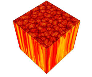
With reference to figure 1, we consider a three-dimensional fluid-saturated porous medium with uniform porosity  $\phi$ and uniform permeability $\kappa$. The origin of the coordinate system is located at the bottom of the domain, and the $x^*,z^*$ axes point along the two horizontal directions, whereas the $y^*$ axis points along the vertical direction (along which gravity $g$ is directed). A positive temperature difference ${\rm \Delta} \theta ^{*}=\theta ^{*}_{max}-\theta ^{*}_{min}$ is maintained between the top and the bottom boundaries by heating the flow from the bottom and cooling it from the top. We consider that fluid density, $\rho ^{*}$, is a linear function of temperature
 \begin{equation} \rho^{*}(\theta^{*})=\rho^{*}(\theta^{*}_{min})-{\rm \Delta}\rho^{*} \frac{\theta^{*}-\theta^{*}_{min}}{\theta^{*}_{max}-\theta^{*}_{min}}, \end{equation}
with  ${\rm \Delta} \rho ^{*}=\rho ^{*}(\theta ^{*}_{min})-\rho ^{*}(\theta ^{*}_{max})$. Assuming validity of the Boussinesq approximation (Landman & Schotting Reference Landman and Schotting2007; Zonta & Soldati Reference Zonta and Soldati2018), the flow is incompressible and governed by Darcy's law
 \begin{equation} \boldsymbol{\nabla}\boldsymbol{\cdot}\boldsymbol{u}^{*}=0,\quad \boldsymbol{u}^{*}={-}\frac{\kappa}{\mu}\left(\boldsymbol{\nabla} P^{*}+\rho^{*}g \boldsymbol{j}\right), \end{equation}
with  $\mu$ the fluid viscosity (constant), $\boldsymbol {u}^{*}=(u^{*},v^{*},w^{*})$ the volume-averaged velocity field, $P^{*}$ the pressure and $\boldsymbol {j}$ the vertical unit vector.
Sketch of the computational domain – with dimensions  $l_{x}^{*}$, $l_{y}^{*}$ and $l_{z}^{*}$ – used to study Rayleigh–Darcy convection. The flow is heated at the bottom, $\theta ^*(y^*=0)=\theta ^*_{{max}}$ and cooled at the top, $\theta ^*(y^*=l^*_{y})=\theta ^*_{{min}}$, and boundaries in the $x^*$ and $z^*$ directions are assumed to be periodic. The gravitational acceleration ( $\boldsymbol {g}$) points downwards. The temperature distribution $\theta ^*$ for the case $Ra=8\times 10^4$ is also shown for illustrative purposes on the side boundaries and in a plane close to the top boundary (specifically, at a distance of $50l_y^*/Ra$ from the top boundary).

The evolution of the temperature field is controlled by the advection–diffusion equation
 \begin{equation} \phi\frac{\partial \theta^{*}}{\partial t^{*}}+\boldsymbol{\nabla} \boldsymbol{\cdot}(\boldsymbol{u}^{*}\theta^{*}-\phi D \boldsymbol{\nabla}\theta^{*})=0, \end{equation}
where  $t^{*}$ is time, and $D$ is the thermal diffusivity, which is considered constant here. The superscript $^{*}$ is used to indicate dimensional variables. The top and bottom boundaries are impermeable and isothermal. Periodicity is assumed in the directions parallel to the boundaries.
2.1. Dimensionless equations
For the present flow configuration, in which buoyancy forces drive the primary flow motion in the vertical direction, natural velocity, temperature and length reference scales are the temperature difference,  ${\rm \Delta} \theta ^{*}$, the buoyancy velocity $V^{*}=g {\rm \Delta} \rho ^{*} \kappa / \mu$ and the domain height, $l_{y}^{*}$, respectively (Fu, Cueto-Felgueroso & Juanes Reference Fu, Cueto-Felgueroso and Juanes2013; Wen et al. Reference Wen, Akhbari, Zhang and Hesse2018). Accordingly, dimensionless variables read as
 \begin{equation} \boldsymbol{u}=\frac{\boldsymbol{u}^{*}}{V^{*}},\quad \theta=\frac{\theta^{*}-\theta^{*}_{min}}{{\rm \Delta} \theta^{*}},\quad t=\frac{t^{*}}{\phi l^{*}_{y}/V^{*}},\quad P=\frac{P^{*}}{{\rm \Delta} \rho^{*}gl^{*}_{y}}. \end{equation}
Introducing the reduced pressure  $p^{*}$, we obtain the dimensionless form of the governing equations (2.3)–(2.2a,b)
 $$\begin{gather} \frac{\partial \theta}{\partial t}+\boldsymbol{\nabla} \boldsymbol{\cdot} \left(\boldsymbol{u}\theta -\frac{1}{Ra} \boldsymbol{\nabla} \theta\right)=0, \end{gather}$$
 $$\begin{gather}\boldsymbol{\nabla}\boldsymbol{\cdot}\boldsymbol{u}=0,\quad \boldsymbol{u}={-}\left(\boldsymbol{\nabla} p -\theta \boldsymbol{j}\right), \end{gather}$$
where  $Ra=g {\rm \Delta} \rho ^{*} \kappa l_{y}^{*} / (\phi D \mu )=V^{*} l^{*}_{y} / (\phi D)$ is the Rayleigh–Darcy number. The boundary conditions for velocity and temperature then read as
 $$\begin{gather} v(y=0)=0,\quad \theta(y=0)=1, \end{gather}$$
 $$\begin{gather}v(y=1)=0,\quad \theta(y=1)=0. \end{gather}$$
 Naturally, the previous choice of reference scales in not unique. A suitable, alternative choice is to take  ${x}_{d}^{*}=\phi D/V^{*}$ as a reference length scale (while keeping the same reference temperature and velocity scales). This gives the so-called diffusive–convective scaling, in contrast with the convective scaling presented above. From a physical viewpoint, ${x}^{*}_{d}$ denotes the length over which advection and diffusion balance (Slim Reference Slim2014), and is independent of the physical domain thickness. When rescaled in the latter way, dimensions are bound in the range ${x}^{*}/{x}_{d}^{*}\in [0,Ra]$, and comparison between simulations at different $Ra$ is easier. For this reason, lengths in this paper are rescaled with respect to $x_{d}^{*}$. Furthermore, introduction of this length scale also yields another interpretation of the Rayleigh–Darcy number, $Ra=l_y^*/{x}_{d}^{*}$, which may be regarded as the dimensionless height of the domain (Slim Reference Slim2014).
2.2. Computational details
The numerical simulations rely on a modified version of a second-order finite-difference incompressible flow solver, based on staggered arrangement of the flow variables (Orlandi Reference Orlandi2000), which has been extensively used for direct numerical simulation of wall-bounded neutrally buoyant and unstably stratified turbulent flows (Pirozzoli Reference Pirozzoli2014; Pirozzoli et al. Reference Pirozzoli, Bernardini, Verzicco and Orlandi2017). The temperature transport equation is advanced in time by means of a hybrid third-order low-storage Runge–Kutta algorithm, whereby the convective terms are handled explicitly and the diffusive terms are handled implicitly, limited to the vertical direction. This approach guarantees that the total temperature variance is discretely preserved in the limit of inviscid flow. A special strategy is used here for the solution of the forced Darcy system (2.5)–(2.6a,b). As in the classical fractional-step algorithm for convection–diffusion equations (Kim & Moin Reference Kim and Moin1985), and exploiting linearity of the equations, at each Runge–Kutta sub-step a provisional velocity field  $\widehat {\boldsymbol {u}}$ is first determined by disregarding pressure, namely
 \begin{equation} \widehat{\boldsymbol{u}} = \theta \boldsymbol{j}, \end{equation}
which is then projected to the space of divergence-free vector functions through a correction step,
 \begin{equation} \boldsymbol{u} = \widehat{\boldsymbol{u}} - \boldsymbol{\nabla} \varphi,\quad \text{with}\ \nabla^2 \varphi = \boldsymbol{\nabla}\boldsymbol{\cdot} \widehat{\boldsymbol{u}}, \end{equation}
and  $\partial \varphi / \partial y = 0$ at boundaries to satisfy the impermeability condition. It is easy to show that the fractional-step procedure (2.8)–(2.9) is equivalent to the original Darcy problem, with $\varphi \equiv p$ and under free-slip boundary conditions. An efficient direct algorithm, based on Fourier expansions along periodic directions (Kim & Moin Reference Kim and Moin1985; Orlandi Reference Orlandi2000), is used here for solving the resulting Poisson equation.
The mesh spacing in the directions parallel to the boundaries was decided based on preliminary grid-resolution studies at low  $Ra$ and inspection of the temperature spectra, to prevent any energy pile up at the smallest resolved flow scales. Regarding the resolution in the vertical direction, we have followed the criterion that twenty points should be placed within the thermal boundary layer edge, identified through the peak location of the temperature variance, and grid points are clustered towards the boundaries using a hyperbolic tangent stretching function. Given the expected linear growth of the temperature gradients, the number of points in each coordinate direction was increased proportionally to $Ra$. The time step is selected so that the Courant–Friedrichs–Lewy number is about unity for all the simulations herein reported. Calculations, carried out at $Ra \le 5\times 10^{3}$, have shown excellent agreement with the numerical results obtained by Hewitt et al. (Reference Hewitt, Neufeld and Lister2014), obtained with a different numerical method.
3. Scaling of the Nusselt number with the Rayleigh number
The key response parameter in Rayleigh–Darcy convection is the Nusselt number ( $Nu$), which controls the relative effect of convection over conduction.
The Nusselt number is evaluated here as the time-averaged value – denoted by angular brackets – of the mean temperature gradient at the top and bottom boundaries,
 \begin{equation} Nu={-}\left \langle \frac{1}{2 \left( l_z l_x\right)} \int_{0}^{l_z}\int_{0}^{l_x} \left[\left.\frac{\partial \theta}{\partial y}\right\rvert_{y=0}+ \left.\frac{\partial \theta}{\partial y}\right\rvert_{y=1}\right] \text{d}x\,\text{d}z \right \rangle. \end{equation}
Measurements of  $Nu$ at various $Ra$ are listed in table 1, and plotted in compensated form ( $Nu/Ra$) in figure 2(a), for $1\times 10^3\le Ra\le 8\times 10^4$. Together with the numerical results obtained in the present three-dimensional (filled circles) and two- dimensional (filled diamonds) studies, we also report results available from previous literature (Hewitt et al. Reference Hewitt, Neufeld and Lister2014, for the three-dimensional case); (Hewitt et al. Reference Hewitt, Neufeld and Lister2012; Wen et al. Reference Wen, Corson and Chini2015; De Paoli et al. Reference De Paoli, Zonta and Soldati2016, for the two-dimensional case). For the two-dimensional case, all the results generally agree, indicating that the scaling proposed by Hewitt et al. (Reference Hewitt, Neufeld and Lister2012), namely $Nu \sim 0.0069 Ra +2.75$, reproduces fairly well not only the asymptotic behaviour of the flow, which sets in already at $Ra \sim 3\times 10^4$, but also the pre-asymptotic behaviour. The situation is more involved in the three-dimensional case, with our data showing no attainment of the expected asymptotic linear behaviour, even at $Ra = 8\times 10^4$. Hewitt (Reference Hewitt2020) provided phenomenological arguments, based on the results of Malkus (Reference Malkus1954) and Howard (Reference Howard1964), that the scaling should be linear. This agrees also with the best known theoretical upper bound, for which $Nu\le 0.0297Ra$ (Otero et al. Reference Otero, Dontcheva, Johnston, Worthing, Kurganov, Petrova and Doering2004). Best fitting of our data, in combination with these observations, yields the scaling (solid line, see also Pirozzoli et al. (Reference Pirozzoli, De Paoli, Zonta and Soldati2021), for further details)
 \begin{equation} Nu/Ra=0.0081 + 0.067 Ra^{{-}0.39}. \end{equation}
Of course, a scaling with a leading term other than linear would result in inconsistent prediction in the ultimate regime. On the other hand, the additional sublinear correction in figure 2(a) has influence only at moderate  $Ra$, becoming negligibly small at high $Ra$, and leaving the stage to the asymptotic linear trend, which we extrapolate to be $Nu=0.0081Ra$. Compared with other correlations found in the literature (Hewitt et al. Reference Hewitt, Neufeld and Lister2014), the present one works fairly well over a rather large range of $Ra$, starting from $Ra \sim 2.5 \times 10^3$. Some discrepancy between the present correlation and the numerical results is observed at $Ra=10^3$, which is, however, to be expected, as our fit is constructed to capture the behaviour of the system in the high- $Ra$ region of the parameter space. It is noteworthy that we estimate – evaluating the point at which the sublinear correction becomes negligibly small (less than 5 %) compared with the leading linear term – the ultimate regime to set in at $Ra \approx 5 \times 10^5$, i.e. well beyond previous predictions.
(a) Compensated Nusselt number as a function of Rayleigh number. Results obtained by Pirozzoli et al. (Reference Pirozzoli, De Paoli, Zonta and Soldati2021) and present numerical simulations are shown by filled circles ( $\bullet$) and diamonds ( ${\blacklozenge}$) for three-dimensional and two-dimensional simulations, respectively. The black solid line indicates the proposed correlation $Nu/Ra=0.0081 + 0.067 Ra^{-0.39}$ (see also Pirozzoli et al. Reference Pirozzoli, De Paoli, Zonta and Soldati2021). Data obtained in previous works, in both two-dimensional (Hewitt et al. Reference Hewitt, Neufeld and Lister2012; Wen et al. Reference Wen, Corson and Chini2015; De Paoli et al. Reference De Paoli, Zonta and Soldati2016) ( $\square$, $\triangledown$ and $\triangleright$, respectively) and three-dimensional (Hewitt et al. Reference Hewitt, Neufeld and Lister2014) ( $\triangle$) simulations are shown with open symbols. The scaling law $Nu/Ra=0.0069+2.75/Ra$ proposed by Hewitt et al. (Reference Hewitt, Neufeld and Lister2012) for the two-dimensional case is shown with a solid red line. Modifications of the flow structure with $Ra$ are shown in the insets, in terms of the temperature distribution in vertical slices at $Ra=10^{3}$ (b), $Ra=10^{4}$ (c) and $Ra=8\times 10^{4}$ (d).

Summary of numerical simulations performed in the present study. For each simulation, we explicitly report Rayleigh number  $Ra$, domain size $l_{x}/l_{y}\times l_{z}/l_{y}\times 1$ and grid resolution $N_{x}\times N_{z}\times N_{y}$. Additional simulations at $Ra=1\times 10^4$, not reported here, have been run for 5 different values of the aspect ratio (see table 2). Nusselt number, $Nu$, and time- and space-averaged temperature root mean square (rms) at the midplane, $\theta _{{rms}}(y=1/2)$, are also reported.

List of simulations at  $Ra=1\times 10^{4}$ to address influence of domain size and aspect ratio.

The change of  $Nu$ with $Ra$ implies a corresponding change of the flow structure. This is clearly shown in figure 2, where the temperature distribution in a vertical $(z, y)$ section, spanning the entire cell height and located at $x=1/2$, is plotted for $Ra=1000$ (figure 2b), $Ra=10\,000$ (figure 2c) and $Ra=80\,000$ (figure 2d). At $Ra=1000$, the flow is dominated by a pair of rolls with aspect ratio ${\sim }1/2$ whose flanks are marked by tall and strongly coherent ascending and descending plumes. These plumes are generated by boundary layer instabilities which grow and propagate vertically into the flow (Graham & Steen Reference Graham and Steen1994). At higher $Ra$, we observe a more complicated flow structure, with small fingers of light fluid emerging from the bottom boundary and moving upwards, and correspondingly small fingers of heavy fluid descending from the top boundary and moving downwards. Coalescence of these fingers generates larger columnar structures – megaplumes – that dominate the core region of the flow and, driven by buoyancy, reach the opposite boundary. This dynamics will be further clarified upon inspection of the flow structure in horizontal planes (see § 5.1).
4. Temperature statistics
In figure 3(a), we show distributions of the mean temperature  $\varTheta =\lvert \theta _w-\theta \lvert$ as a function of the distance from the boundary ( $y$) in semi-log scale, for the various $Ra$ considered in this study, limited to the lower half of the domain. The rise of $\varTheta$ to the centreline value, $\varTheta =0.5$, occurs almost entirely within a very short distance (say $\delta$) from the boundaries. This distance, which may be regarded as the effective thermal boundary layer thickness, is seen to depend on the value of $Ra$, ranging from $\delta \simeq 10^{-1}$ at $Ra=10^3$, to $\delta \simeq 10^{-3}$ at $Ra=8\times 10^4$. In this outer representation, the temperature profile outside the thermal boundary layer is well fitted with a logarithmic distribution, $\varTheta =A\ln {(2y)}+1/2$, where $A=0.0188$ (dashed blue line in figure 3a). A similar behaviour has been observed in classical Rayleigh–Bénard convection (Ahlers et al. Reference Ahlers, Bodenschatz, Funfschilling, Grossmann, He, Lohse, Stevens and Verzicco2012). Restricting to a region closer to the central part of the domain ( $0.45\le y \le 0.55$), Hewitt et al. (Reference Hewitt, Neufeld and Lister2014) observed that the temperature profile scales linearly with $y$. This observation holds also in the present case. When $\varTheta$ is plotted as a function of the rescaled vertical distance, $y \times Nu$ (see figure 3b), all profiles collapse in the near-boundary region, up to $y \times Nu \approx 1$, where they nicely follow the expected linear behaviour $\varTheta =y\times Nu$ (dashed line). This is a strong indication that the thickness $\delta$ of the thermal boundary layer scales well with $Nu$, at all $Ra$.
$Ra$.
(a) Time- and horizontally averaged temperature  $\varTheta = \lvert \theta _{w}-\theta \lvert$, where $\theta _{w}$ is the boundary temperature. Profiles are shown as a function of the vertical coordinate, $y$ (a), and as a function of the vertical coordinate rescaled by the Nusselt number, $y\times Nu$ (b). Colours correspond to the Rayleigh number, from low (white) to high (black). Due to symmetry of the problem, only half of the domain is shown. In the bulk of the domain, the profiles exhibit a logarithmic scaling, $\varTheta =A\ln {(2y)}+1/2$, with $A=0.0188$ (dashed blue line). When the wall-normal coordinate is rescaled by the Nusselt number, $y\times Nu$ (b), all temperature profiles are self-similar and are well described by a linear function, $\varTheta =y\times Nu$ (dashed blue line), near the boundary.

Interestingly, the behaviour of  $\varTheta$ is non-monotonic with $y$, and it develops a local maximum around the edge of the thermal boundary layer, say $0.5 < y \times Nu < 5$ in rescaled units (figure 3b). This maximum is especially visible at $Ra=10^3$, whereas it weakens at higher $Ra$. Such non-monotonic behaviour of $\varTheta$ bears important consequences on the heat transport mechanisms across the porous domain, as the diffusive heat flux $q_{\theta } \propto \text {d} \theta /\text {d} y$ may become negative. This is explicitly quantified in figure 4, where we show the rescaled mean temperature gradient, $-Nu^{-1} \text {d} \theta /\text {d} y$, as a function of $y$ (figure 4a) and as a function of $y \times Nu$ (figure 4b), at various $Ra$. Based on these plots, one can evaluate quite precisely the thickness of the thermal boundary layer $\delta$, identified as the location where the temperature gradient becomes negligibly small. We are now able to confirm the estimates given in figure 3, with the boundary layer thickness ranging from $\delta \simeq 10^{-1}$ for $Ra=10^3$, to $\delta \simeq 10^{-3}$ for $Ra=8\times 10^4$. In rescaled units (figure 4b), this corresponds to $\delta \times Nu \simeq 1$, i.e. $\delta \simeq 1/Nu$. As anticipated above, at small $Ra$ the diffusive heat flux can become negative (at the edge of the thermal boundary layer, around $y \times Nu \simeq 1$), thus indicating the presence of regions where the local mean temperature gradient is opposite to the imposed gradient (these regions are usually called counter-gradient flux regions, see also Zonta & Chibbaro (Reference Zonta and Chibbaro2016) and Hadi Sichani et al. (Reference Hadi Sichani, Marchioli, Zonta and Soldati2020) for further details). A similar overshoot in the temperature profiles at the edge of the thermal boundary layer were also observed in Rayleigh–Bénard convection at high Prandtl number (Schmalzl, Breuer & Hansen Reference Schmalzl, Breuer and Hansen2002). The existence of such regions may be ascribed to the fact that, when $Ra$ is small, the vertical plumes carry their momentum and temperature almost unchanged all across the fluid layer. As a consequence, there are regions close to the bottom boundary in which the temperature is nearly the same as at the top boundary, and vice versa, which imply local temperature inversion. This effect tends to vanish as $Ra$ increases, as a consequence of the vigorous mixing that homogenizes the temperature field, and greatly weakens the temperature gradients. Alternatively, the absence of counter-gradient flux regions for increasing $Ra$ can be explained by considering that the height of the porous domain, in dimensionless diffusive units, is $l_y=Ra$, which suggests that the influence of one boundary on the other becomes weaker and weaker as $Ra$ increases (i.e. the boundaries are effectively farther apart).
(a) Vertical temperature gradient ( $-\mathrm {d}\theta /\mathrm {d}y$) normalized by the Nusselt number, $Nu$ (half-domain is shown). Profiles are shown as a function of the vertical coordinate, $y$ (a), and as a function of the vertical coordinate normalized by the Nusselt number, $y\times Nu$ (b). Colours correspond to the Rayleigh number, from low (white) to high (black). The dashed blue line denotes the zero value.

The root mean square distributions of the temperature fluctuations  $\theta _{rms}$ are shown in figure 5. Consistently with observations made above regarding the mean temperature and its gradient, temperature fluctuations increase sharply in a thin region near the boundary, until they develop a peak at a distance between $y \simeq 10^{-1}$ for $Ra=10^3$, and $y \simeq 10^{-3}$ for $Ra=8\times 10^4$. The magnitude of the peak weakly decreases with $Ra$, as shown in figure 6a). Past the peak, $\theta _{rms}$ decreases and it tends to level off towards the centre of the domain. Universality is near perfect in the central part of the domain, where, in agreement with the findings of Hewitt et al. (Reference Hewitt, Neufeld and Lister2014), we get $\theta _{rms}\approx 0.1$, quite robustly across the $Ra$ range. Again, when $\theta _{rms}$ is shown as a function of $y\times Nu$, all the profiles are satisfactorily universal towards the boundary. The location at which temperature fluctuations attain a peak (shown in figure 6b) is frequently used to estimate the thermal boundary layer thickness (Ahlers, Grossmann & Lohse Reference Ahlers, Grossmann and Lohse2009). In line with our previous estimates based on other observables (i.e. mean temperature and mean temperature gradient), we find that $\delta \approx 1/Nu$, although the scaling only becomes clear at $Ra \gtrsim 10^4$.
(a) Time- and horizontally averaged root-mean-square temperature distributions (half-domain is shown). Profiles are shown as a function of  $y$ (a), and as a function of $y\times Nu$ (b). Colours correspond to the Rayleigh number, from low (white) to high (black). The maximum value obtained for $Ra=2.5\times 10^{3}$ is marked with a horizontal dashed line.

Peak value (a) and peak location (b) of time- and horizontally averaged root-mean-square temperature distributions, respectively defined as  $\theta _{rms}$ and $y_{m}$.

5. Flow structures
5.1. Flow structures near the boundaries
The identification of coherent flow structures is a crucial aspect in many branches of fluid mechanics. In buoyancy-driven flows, coherent flow structures are often identified based on the behaviour of temperature fluctuations or of temperature–velocity correlations. Unlike in Rayleigh–Bénard turbulence – in which use of the different identification techniques can lead to different results (Krug, Lohse & Stevens Reference Krug, Lohse and Stevens2020) – in Rayleigh–Darcy convection all these criteria yield similar results (De Paoli et al. Reference De Paoli, Zonta and Soldati2016). Of specific importance is the characterization of the flow structure in the region near the flow boundary, which we do in figure 7 by inspecting the temperature distribution in a horizontal plane located near the bottom boundary, at  $y=50/Ra$, for the $Ra_{80}$ simulation, since the flow features we wish to discuss are emphasized at the highest $Ra$. Short, thin and bright filaments, corresponding to warm fluid protoplumes ejected from the bottom boundary, are interconnected and arranged into an organized pattern of small polygonal-shaped cells (Fu et al. Reference Fu, Cueto-Felgueroso and Juanes2013; Amooie, Soltanian & Moortgat Reference Amooie, Soltanian and Moortgat2018). Those cells enclose dark regions of colder return fluid which replace the ejected hot fluid. Upon impingement on the boundary, cold fluid is deflected in the horizontal directions and pushes newly formed protoplumes to interact, giving rise to a dynamic pattern, in which some of the protoplumes cluster into specific regions – thicker bright ridges, see figure 7(a) – which define the boundaries of larger superstructures – almost homogeneously distributed over the plane – from which larger buoyant plumes are ejected.
(a) Temperature distributions in a plane close to the bottom boundary  $(x,y=50/Ra,z)$ for the $Ra_{80}$ simulation. (b) Close-up view of the temperature distribution in a square subdomain. (c) Filtered temperature field, highlighting the plume organization in the near-boundary region.

We now aim at achieving a more quantitative description of the flow structure organization described above, while leaving detailed characterization of supercells to § 5.3. For that purpose, in figure 7(c) we only retain those points where  $\theta >3/4$ (see discussion in the Appendix), yielding a binarized representation in which the protoplumes show up as black filaments encircling elementary flow cells, which can therefore be considered as minimal flow units (Fu et al. Reference Fu, Cueto-Felgueroso and Juanes2013).
Based on the binarized maps thus obtained (figure 7c), we measure the area of all subdomains bounded by filamentary protoplumes, and we evaluate their corresponding probability density distribution  $P(A)$, as shown in figure 8(a). Here, lengths are expressed in dimensionless units as $L_x=l_x^*/x_d^*$ and $L_z=l_z^*/x_d^*$, hence areas range in the interval $0< A<Ra^2$. Regardless of the specific value of $Ra$, the probability density distributions have similar shapes. We found large probability density of regions with very small area, $A/Ra^2 \sim 10^{-1}\div 10^{-6}$ (i.e. having side $l \sim 10^{-1}\div 10^{-3}$), depending on $Ra$. The probability of observing cells with increasing area drops off rapidly. Note that, while the probability density distributions for $Ra>2\times 10^4$ seem to collapse fairly well, some differences are found at lower $Ra$, with lower probability of having smaller cells, and higher probability of having larger cells (this is particularly apparent at $Ra = 10^3$). This observation suggests that the structure and organization of the flow cells near the boundary are still evolving within the investigated range of $Ra$, although the evolution becomes milder and milder as $Ra$ increases. Not only is the extension of flow cells important, but also their shape, which we characterize by computing the cell circularity parameter, ${\mathcal {C}}=4{\rm \pi} A / \varPi ^2$, with $\varPi$ the cell perimeter. The corresponding probability density distributions are shown in figure 8(b). Note that ${\mathcal {C}}=1$ in the case of circular regions, whereas ${\mathcal {C}} \to 0$ in the case of highly elongated, needle-shaped regions. All other possible shapes range between those two limiting values, as visually rendered at the bottom horizontal axis of figure 8(b). For all $Ra$ here considered, the probability density function of ${\mathcal {C}}$ shows a qualitatively similar distribution, with maximum probability density of observing regions with circularity ${\mathcal {C}}\sim 0.8$, as is the case for nearly square cells. However, the probability of observing near-circular regions is non-negligible, as P $({\mathcal {C}}=1)\sim 0.3$. Elongated regions (say, ${\mathcal {C}} < 0.2$) are quite frequent at low $Ra$, and in particular at $Ra=10^3$, but they become increasingly rare at high $Ra$. In line with the previous discussion on $P(A)$, it is interesting to observe that $P({\mathcal {C}})$ is still evolving within the range of $Ra$ investigated here, but it seems to tend towards an asymptotic distribution for increasing $Ra$. In § 5.4, the dependence of our results on the domain size has been tested by performing simulations at $Ra=10^4$ in boxes with various sizes.
Characterization of flow structures in the near-boundary region. Structures are identified based on the binarized temperature maps, as shown in figure 7(c). (a) Probability density distribution of cells area; (b) probability density distribution of the cell circularity parameter,  ${\mathcal {C}}=4{\rm \pi} A/ \varPi ^2$, with $\varPi$ the cell perimeter. All quantities are expressed in dimensionless units (the domain size is $l_x=l_z=Ra$). Examples of shapes, associated with the corresponding values of circularity, are also reported at the bottom of (b).

5.2. Identification of supercells and dominant length scales in Rayleigh–Darcy convection
As previously discussed – and similar to what is observed in classical Rayleigh–Bénard turbulence (Stevens et al. Reference Stevens, Blass, Zhu, Verzicco and Lohse2018; Green et al. Reference Green, Vlaykov, Mellado and Wilczek2020; Krug et al. Reference Krug, Lohse and Stevens2020; Berghout, Baars & Krug Reference Berghout, Baars and Krug2021) –, the near-boundary region of the Rayleigh–Darcy flow at high  $Ra$ is characterized by the presence of large-scale, long-lived coherent structures called ‘supercells’ resulting from coalescence of smaller primary cells.
To analyse the behaviour of the supercells, we again consider the temperature distribution in the near-boundary region,  $\theta (x,y=50/Ra,z)$, as shown in figure 9(a) for the $Ra_{80}$ simulation. Thick, bright ridges identifying high-temperature regions, and marking the boundary of supercells, emerge rather clearly. Monitoring the time evolution of the flow, it appears that the boundaries of the supercells are quite stationary, showing limited lateral shift. However, their interior is characterized by the presence of smaller cells (figure 9a), which continuously form, move and merge, although remaining confined within the boundaries of the corresponding supercell. Hence, to better highlight the time persistence of the supercells, we have computed averages of the temperature field over a one hundred flow samples, spaced ${\rm \Delta} t_{av} \simeq 0.1$ apart. The time window has been carefully selected to be much larger than the time scale of the small protoplumes populating the boundary layer (typically, ${\rm \Delta} t \sim {{O}} (10^{-2})$), which will thus be filtered, but smaller than the time scale of large megaplumes (typically, ${\rm \Delta} t \sim {{O}} (1)$). The results of the averaging procedure are shown in figure 9(b), which makes the boundaries of the supercells much more evident.
Detection of supercells in the near-boundary region: (a) instantaneous temperature distribution at  $y=50/Ra$ for the $Ra_{80}$ simulation, in which supercells are identified by their bright, high-temperature boundaries; (b) time-averaged temperature field. Whereas the boundary of supercells is relatively stable, with no remarkable change in time and space, the inner portion is controlled by smaller cells, which continuously form and merge with the existing ones, while remaining mostly confined within bounding supercells.

In order to gain a perception to the flow organization along the vertical direction, in figure 10 we compare the temperature fields in a near-wall plane and at the flow centreplane, at various  $Ra$. The flanks of the supercells (figure 10a–d) become more and more evident as $Ra$ increases, and the typical size of cells and supercells decreases distinctly when expressed in convective units, based on the thickness of the porous layer and on the buoyancy velocity. Note, however, that, when expressed in terms of the diffusive–convective scaling (see § 2), the horizontal area of the top and bottom boundaries for the $Ra_{80}$ simulation is 64 times larger than for the $Ra_{10}$ simulation, with obvious influence on the area of each flow cell. A similar trend for the characteristic size of the flow structure, i.e. flow structures which reduce in size at increasing $Ra$ when shown in dimensionless convective units, is also observed at the flow centreplane, see figure 10(e–h). However, and different from what happens near the boundary, no signature of small-scale structures is evident at the centreplane, which is dominated by tall columnar megaplumes which span the whole flow thickness, and which are clearly visible as vertical yellow stripes in figure 2(b–d).
Temperature distributions in a near-boundary plane (a–d) and in the flow centreplane (e–h).

Obtaining a quantitative estimate of the size of the dominant flow structures near the boundaries and at the flow centreplane is obviously important on account of their influence on the overall heat transfer mechanisms. For that purpose we consider the two-dimensional spectral density of the temperature field,  $E(k_x,k_z)$, where $k_x,k_z$ are the horizontal wavenumbers, and we define a mean radial wavenumber as (Hewitt et al. Reference Hewitt, Neufeld and Lister2014)
 \begin{equation}
\overline{k}_r(y)=\left\langle
\frac{\displaystyle\int\int\sqrt{k_{x}^{2}+k_{z}^{2}}E(k_{x},k_{z})\,\mathrm{d}x\,\mathrm{d}z}
{\displaystyle\int\int
E(k_{x},k_{z})\,\mathrm{d}x\,\mathrm{d}z}\right\rangle.
\end{equation}
\begin{equation}
\overline{k}_r(y)=\left\langle
\frac{\displaystyle\int\int\sqrt{k_{x}^{2}+k_{z}^{2}}E(k_{x},k_{z})\,\mathrm{d}x\,\mathrm{d}z}
{\displaystyle\int\int
E(k_{x},k_{z})\,\mathrm{d}x\,\mathrm{d}z}\right\rangle.
\end{equation}
The latter quantity can then be interpreted as a measure of the inverse size of the dominant structures at a given vertical position. The values of  $\overline {k}_r$ in the near-wall plane and at the flow centreplane are reported in figure 11 as a function of $Ra$.
$Ra$.
Mean radial wavenumber  $\overline {k}_{r}$ (solid lines and symbols) of the temperature distribution, determined after (5.1). The results computed in the centre ( $y=1/2$, filled symbols) and in the near-boundary region ( $y=50/Ra$, empty symbols) are reported. The best fits obtained (dashed lines) are $\overline {k}_{r}=0.25Ra^{0.49}$ and $\overline {k}_{r}=0.045Ra^{0.81}$, for the centre and near-boundary regions, respectively.

Near the boundary, power-law fitting of the simulation data for  $10^{3}\le Ra\le 8\times 10^{4}$, yields the scaling
 \begin{equation} \overline{k}_r(y=50/Ra) \approx 0.045Ra^{0.81}, \end{equation}
where taking a 95 % confidence interval, the value of the fitting exponent is  $0.8057 \pm 0.0174$. This result seems to fall short of the linear scaling reported by Hewitt et al. (Reference Hewitt, Neufeld and Lister2014), which was arrived at by assuming that the horizontal size of the near-boundary plumes scales with the boundary layer thickness, hence as ${\sim }1/Nu$. Given that, in the ultimate regime, $Nu\sim Ra$, it would follow that $\overline {k}_r\sim Ra$. However, in our previous work (Pirozzoli et al. Reference Pirozzoli, De Paoli, Zonta and Soldati2021) we noticed that such ultimate regime would probably set in at $Ra\approx 5\times 10^{5}$, well beyond the range of $Ra$ currently accessible to numerical simulations. Hence, deviations from such asymptotic scaling are plausible.
At the flow centreplane, data fitting of our results yields
 \begin{equation} \overline{k}_r(y=1/2) \approx 0.25Ra^{0.49}, \end{equation}
where taking a 95 % confidence interval, the fitting exponent is  $0.4893 \pm 0.0231$. This is now in excellent agreement with previous theoretical predictions ( $\overline {k}_r\sim Ra^{1/2}$, Hewitt & Lister Reference Hewitt and Lister2017) and with simulations ( $\overline {k}_r=0.17Ra^{0.52}$, Hewitt et al. Reference Hewitt, Neufeld and Lister2014). This suggests that the size and spacing of the dominant structures at the centreplane scale well with previous predictions of the flow structure organization that maximizes the vertical heat transport (Hassanzadeh, Chini & Doering Reference Hassanzadeh, Chini and Doering2014)
5.3. Supercells and megaplumes
To further connect flow structures near the boundary (supercells) with flow structures in the core (megaplumes), we apply a low-pass filter (with cutoff wavenumber  $k_c$) to the near-boundary temperature distribution, so as to remove small-scale structures (Krug et al. Reference Krug, Lohse and Stevens2020). Given our goal of linking the near-boundary flow structures to those at the core, we set the cutoff wavenumber to coincide with the mean radial wavenumber at the centreplane, i.e. $k_{c}=\overline {k}_{r}(y=1/2)$, as prescribed by (5.3). Results are shown in figure 12 for Rayleigh numbers in the low-to-moderate region, namely $Ra=10^3, 5\times 10^3, 10^4$ (with same dimensionless size, $l_x/l_y\times l_z/l_y = 4 \times 4$, see table 1), in which the flow changes significantly, whereas changes are minimal at higher $Ra$. A one-to-one comparison between the filtered temperature field in the near-boundary region ( $\theta _{f}$) and in the flow centreplane is provided in figure 12(d–i), where a the temperature iso-line $\theta =1/2$ in the centreplane is also superposed on the contour maps. At $Ra=10^3$, we note close correspondence between the filtered near-boundary temperature distribution (figure 12d) and the unfiltered distribution in the centreplane (figure 12g), which, however, seems to weaken at higher $Ra$ (see figure 12f,i).
Temperature distributions at  $y=50/Ra$ from the top boundary (a–c), corresponding low-pass filtered distributions (d–f) and temperature distribution in the centreplane (g–i). Three values of the Rayleigh number are considered, namely $1\times 10^3$ (a,d,g), $5\times 10^3$ (b,e,h) and $1\times 10^4$ (c, f,i). The $\theta =1/2$ iso-line in the centreplane is also shown as a black solid line in the near-wall filtered (d–f) and centreplane (g–i) temperature distributions. The domain size is $l_x=l_z=4l_y$ for all cases.

A quantitative evaluation of the similarities between the unfiltered temperature field at the centreplane ( $\theta$) and the filtered temperature field near the boundary ( $\theta _{f}$), is provided by their correlation coefficient, namely
 \begin{equation} r=\left\langle\frac{\displaystyle\int\int \left(\theta-\overline{\theta}_{f}\right)\left(\theta_{f}-\overline{\theta}_{f}\right) \mathrm{d}x\,\mathrm{d}z}{\displaystyle\sqrt{\int\int \left(\theta-\overline{\theta}_{f}\right)^{2} \mathrm{d}x\,\mathrm{d}z}\sqrt{\int\int \left(\theta_{f}-\overline{\theta}_{f}\right)^{2} \mathrm{d}x\,\mathrm{d}z}}\right\rangle, \end{equation}
which we determine by averaging in time the correlation coefficients found in the instantaneous temperature fields. This is shown in figure 13 as a function of  $Ra$, and found to be maximum at the lower $Ra$ (a peak value $r\sim 0.75$ is found at $Ra=10^3$), and to slowly relax to a value $r\approx 0.4$ for $Ra \ge 2\times 10^4$. This is a further confirmation that supercells are the footprint of the megaplumes which dominate the core part of the flow.
Correlation factor between unfiltered centreplane temperature and filtered near-wall temperature, as defined in (5.4), as a function of  $Ra$. Simulations with $l_x/l_y=l_z/l_y=1$ ( $Ra>10^{4}$) and with $l_x/l_y=l_z/l_y=4$ ( $Ra\le 10^{4}$) are reported.

5.4. Assessment of domain size effects
A series of additional simulations – whose parameters are summarized in table 2 – has been carried out to explore the effect of computational box size and aspect ratio. In particular – figure 14 – we look at the intertwined behaviour of the flow structure near the boundary and at the domain centre (by looking at the corresponding temperature contour maps). The strong effect induced by the shrinkage of the domain along the  $x$ direction is clearly visible in figure 14 (see (a–d)). Flow confinement, due to the applied periodicity in a narrow domain, results in streaky structures that are almost perfectly aligned in $x$. Such bias is not present when the aspect ratio is increased (see figure 14g–h). To quantify the influence of the domain size on the flow structure we compute the mean radial wavenumber – as defined in (5.1) – near the boundary and at the domain centre, for different aspect ratios. We recall here that $\overline {k}_r$ – which is proportional to the inverse of a length scale – provides an estimate of the characteristic size of the dominant flow structures. The results, shown in figure 14, clearly demonstrate that the typical size of the flow structures is strongly influenced by the box aspect ratio: going from ${A{\kern-4pt}R} =l_x/l_z=1/8$ to ${A{\kern-4pt}R} =1$, $\overline {k}_r$ monotonically increases – in particular when evaluated in the near-boundary region, until it reaches a maximum value for ${A{\kern-4pt}R} =1$. This value then remains almost constant for further increase of ${A{\kern-4pt}R}$. A similar behaviour, although less pronounced, is also observed for the flow structure at the domain centre. We therefore conclude that, at $Ra=1\times 10^4$, a domain characterized by ${A{\kern-4pt}R} =1$ (i.e. $l_{x}/l_y=l_{z}/l_y=1$) is large enough to properly capture the entire flow structure and therefore to obtain reliable statistics.
Effect of the domain size (horizontal aspect ratio,  ${A{\kern-4pt}R} =l_x/l_z$) on the flow structure at $Ra=1\times 10^{4}$. Seven different aspect ratios in the range $1/8\le {A{\kern-4pt}R} \le 4$ (see table 2 for details) are considered. (a–h) Instantaneous temperature distribution in the near-boundary region – $y=50/Ra$ – (a,c,e,g) and at the flow centreplane – $y=1/2$ – (b,d, f,h) for ${A{\kern-4pt}R} \le 1$. Please note that the colour bars are different for the two regions considered. (i) Mean radial wavenumber $\overline {k}_{r}$ of the temperature distribution at the flow centreplane (filled symbols) and in the near-boundary region (open symbols).

6. Conclusions
We used numerical simulations to study three-dimensional Rayleigh–Darcy convection at Rayleigh–Darcy number,  $Ra$, in the range $1\times 10^3\le Ra\le 8\times 10^4$. We characterized the flow both qualitatively and quantitatively, and we have been able to clearly link the flow structure in the core of the domain to the near-boundary convective cells. The dependence of the Nusselt number $Nu$ – the main response parameter of the flow – with the Rayleigh number $Ra$ is well described by a linear correlation plus a sublinear correction term, whose importance vanishes for increase $Ra$, and asymptotically relaxes – for estimated $Ra$ in excess of $5 \times 10^5$ – into the expected linear behaviour. Temperature statistics clearly showed that the thickness of the thermal boundary layer scales very well with the Nusselt number, $\delta \sim 1/Nu$. When properly rescaled by the Nusselt number, the mean temperature profiles exhibit a self-similar behaviour which, within the boundary layer $\delta$, grows linearly with the vertical distance $y$. We investigated the near-boundary flow structure by looking at the temperature field on a horizontal plane very close to the boundary. The emerging picture is characterized by an organized flow structure composed by small polygonal-shaped cells hierarchically nested together to form larger supercells. Looking at the geometrical properties (area and shape) of such cells near the boundary, we observed that the flow structure near the boundaries is still developing within the range $Ra$ investigated in this study, although it seems to reach an asymptotic self-similar and optimal configuration for increasing $Ra$. Far from the boundaries, the core of the flow is characterized by large columnar temperature structures, which we characterize by means of the mean wavenumber, $\overline {k}_{r}$. In addition, for the flow cells near the boundary, there is a discrepancy between the measured mean wavenumber ( $\overline {k}_{r}\sim Ra^{0.81}$) and the one predicted by the theory ( $\overline {k}_{r}\sim Ra$), possibly due to the fact that the ultimate regime is not attained yet. By contrast, similar measurements performed in the centre of the domain are in excellent agreement with the theoretical predictions $\overline {k}_{r}\sim Ra^{1/2}$, likely indicating that the core region of the flow has reached its asymptotic, ultimate stage. In addition, we establish a link between the near-boundary long-lived coherent structures (supercells) and the columnar structures controlling the interior part of the flow (megaplumes), confirming that the supercells are nothing but the footprint of megaplumes. Finally, we have considered the effect of the domain size on the flow structure. By changing the horizontal domain dimensions, we identified $l_x=l_y=l_z$ as the minimum domain size required to properly resolve the flow structure for $Ra\ge 1\times 10^4$.
Acknowledgements
We acknowledge CINECA supercomputing centre (under grants ISCRA IsB20–3DSIMCON and PRACE Pra21-5415) and Vienna Scientific Cluster (VSC) for generous allowance of computational resources. We also acknowledge late Prof. Charles Doering for very insightful discussions and comments on the work.
Funding
S.P. and F.Z. gratefully acknowledge financial support from ERASMUS+ project 29415-EPP–1–2014–1–IT–EPPKA3–ECHE existing between TU Wien and La Sapienza University. The authors acknowledge the TU Wien University Library for financial support through its Open Access Funding Program.
Declaration of interests
The authors report no conflict of interest.
Appendix. On the identification of plume boundaries
In this appendix we discuss the approach we have followed to identify the plume boundaries and their corresponding shapes. We focus on a plane close to the bottom boundary ( $y=50/Ra$), were we take temperature slices along a horizontal line at $z=1/2$. For ease of discussion, here, we show only a small portion $0\le x/Ra \le 0.2$, i.e. one fifth of the full domain along the $x$ direction. At this position, temperature varies in the range $1/2\le \theta \le 1$, as shown by the blue line in figure 15.
Temperature ( $\theta$, blue) and temperature gradient ( $\partial \theta /\partial x$, red) distributions along a line located on a horizontal plane near the wall $(x,y=50/Ra,z=1/2)$. The values of $x$ corresponding to $\theta =3/4$ (dashed line) are also indicated by grey lines, and correlate well with the location of maximum/minimum $\partial \theta /\partial x$.

We now hypothesize that the boundary of the temperature-carrying flow structures (i.e. plumes) corresponds to locations where temperature gradients are maximum/minimum. To support our hypothesis, we show the behaviour of  $\partial \theta /\partial x$ with a red line in figure 15. Vis-à-vis comparison of $\theta (x)$ (blue line) and $\partial \theta /\partial x$ (red line), makes it clear that locations where $\lvert \partial \theta /\partial x \lvert$ is maximum provide a good indication for the plume boundary. In addition, we note that the maximum of $\lvert \partial \theta /\partial x \lvert$ occurs where $\theta (x)=0.75$ (see dashed line in figure 15). Hence, this condition is retained to identify the near-wall flow cells.


 Open access

