


I. Introduction
Managers provide a great deal of information in order to influence market beliefs and, as a consequence, stock price levels. Beyond standard accounting figures, earnings guidance has become a central tool to shape investor beliefs given its inherently forward-looking nature (Penman (Reference Penman1980), Ball and Shivakumar (Reference Ball and Shivakumar2008)). Consequently, guidance can lead to more efficient stock pricing if value-relevant information is already published at an early stage (Cotter, Tuna, and Wysocki (Reference Cotter, Tuna and Wysocki2006), Seybert and Yang (Reference Seybert and Yang2012)). However, systematic biases in earnings guidance might also impair market efficiency (Johnson, Kim, and So (Reference Johnson, Kim and So2020)). In this article, we argue that managers cater to their investors through earnings guidance by communicating systematically biased information. Based on a simple model, we posit that managers cater to their investors’ perception of firm and management performance by issuing particularly optimistic forecasts if their investors have experienced disappointing stock returns and vice versa. Our empirical analyses support this conjecture. Moreover, we find that such opportunistically biased earnings guidance influences stock market prices and that this effect reverses when the actual earnings are announced at the end of the fiscal year. Analyses based on managerial compensation and tenure suggest that managers, who cater to their investors, benefit.
We formalize our catering theory in a parsimonious model based on three central ingredients. First, markets react to earnings guidance, incorporating conveyed forecasts at least partially into earnings expectations (Ajinkya and Gift (Reference Ajinkya and Gift1984), Beyer (Reference Beyer2009)). Second, loss-averse investors evaluate their stock investments relative to their purchase price, deeming stock prices short of that reference price as disappointing (Kahneman and Tversky (Reference Kahneman and Tversky1979), Shefrin and Statman (Reference Shefrin and Statman1985), and Tversky and Kahneman (Reference Tversky and Kahneman1992)). Third, managers’ utility depends both on the long-term shareholder value and on short-run stock prices as investors might react unfavorably to poor stock returns (Baker and Wurgler (Reference Baker and Wurgler2004), Baker, Mendel, and Wurgler (Reference Baker, Mendel and Wurgler2016)). The model’s central prediction is that managers face strong incentives to convey excessively optimistic forecasts if the firm’s stock trades below the average investor’s purchase price. Thus, we predict a smoothing pattern akin to earnings management: managers issue particularly optimistic forecasts if investors have experienced disappointing stock returns. After high stock returns, managers might issue slightly pessimistic guidance to have some good news in reserve.
To test our theoretical predictions empirically, we employ the capital gains overhang measure
 $ CGO $
as proposed by Grinblatt and Han (Reference Grinblatt and Han2005), which measures the stock return experienced by the firm’s average investor.
$ CGO $
as proposed by Grinblatt and Han (Reference Grinblatt and Han2005), which measures the stock return experienced by the firm’s average investor.
 $ CGO $
reflects the experienced return based on the average investor’s purchase price which is estimated by the use of past stock price and turnover dynamics. It is well established that the purchase price is a highly important reference price for investors such that
$ CGO $
reflects the experienced return based on the average investor’s purchase price which is estimated by the use of past stock price and turnover dynamics. It is well established that the purchase price is a highly important reference price for investors such that
 $ CGO $
strongly influences the evaluation of their investments (see, e.g., Shefrin and Statman (Reference Shefrin and Statman1985), Ben-David and Hirshleifer (Reference Ben-David and Hirshleifer2012), and An, Wang, Wang, and Yu (Reference An, Wang, Wang and Yu2020)). Thus,
$ CGO $
strongly influences the evaluation of their investments (see, e.g., Shefrin and Statman (Reference Shefrin and Statman1985), Ben-David and Hirshleifer (Reference Ben-David and Hirshleifer2012), and An, Wang, Wang, and Yu (Reference An, Wang, Wang and Yu2020)). Thus,
 $ CGO $
is the best-suited variable to proxy for the investors’ perception of stock performance which managers will certainly be acutely aware of, even if they do not directly observe
$ CGO $
is the best-suited variable to proxy for the investors’ perception of stock performance which managers will certainly be acutely aware of, even if they do not directly observe
 $ CGO $
. Hence, we expect
$ CGO $
. Hence, we expect
 $ CGO $
to predict the direction and magnitude of catering via earnings guidance. We examine the impact of
$ CGO $
to predict the direction and magnitude of catering via earnings guidance. We examine the impact of
 $ CGO $
on these systematic biases in earnings forecasts by employing the IBES Guidance database and define the
$ CGO $
on these systematic biases in earnings forecasts by employing the IBES Guidance database and define the
 $ Guidance $
 $ Bias $
as the difference between forecasted earnings per share and ex post earnings realization deflated by the firm’s stock price before the initial guidance.
$ Bias $
as the difference between forecasted earnings per share and ex post earnings realization deflated by the firm’s stock price before the initial guidance.
Consistent with managerial catering, we find that managers of low-
 $ CGO $
firms (bottom 20% of firms) significantly overestimate future earnings with an average
$ CGO $
firms (bottom 20% of firms) significantly overestimate future earnings with an average
 $ Guidance $
 $ Bias $
of 1.16%. On the contrary, managers of high-
$ Bias $
of 1.16%. On the contrary, managers of high-
 $ CGO $
firms (top 20% of firms) tend to insignificantly underestimate earnings with an average
$ CGO $
firms (top 20% of firms) tend to insignificantly underestimate earnings with an average
 $ Guidance $
 $ Bias $
of −0.03%. This understatement among well-performing firms is in line with managers’ desire to guide expectations toward beatable levels (Johnson et al. (Reference Johnson, Kim and So2020)). The negative relationship between
$ Bias $
of −0.03%. This understatement among well-performing firms is in line with managers’ desire to guide expectations toward beatable levels (Johnson et al. (Reference Johnson, Kim and So2020)). The negative relationship between
 $ CGO $
and
$ CGO $
and
 $ Guidance $
 $ Bias $
holds in a multitude of specifications.
$ Bias $
holds in a multitude of specifications.
Our subsequent regression analyses using interaction tests support catering as the underlying mechanism of these systematic biases in management guidance. For example, our model predicts that myopic managers exposed to short-term pressure will engage more strongly in catering. Indeed, the effect of
 $ CGO $
on
$ CGO $
on
 $ Guidance $
 $ Bias $
is stronger among firms with high stock turnover and severe downward price pressure from short sellers. Moreover, we confirm our model’s prediction that catering is stronger among stocks with high return volatility. Furthermore, our model implies that managers cater less as their costs for issuing biased forecasts increase. We argue that the reputational costs of inaccurate forecasts are lower if sophisticated market participants such as analysts fail to reach a consensus about future earnings, and if inaccurate forecasts are made comparably early. As predicted, catering is stronger for firms with a large dispersion in analysts’ earnings forecasts and for guidance that managers convey earlier. Finally, we show that the effect of
$ Bias $
is stronger among firms with high stock turnover and severe downward price pressure from short sellers. Moreover, we confirm our model’s prediction that catering is stronger among stocks with high return volatility. Furthermore, our model implies that managers cater less as their costs for issuing biased forecasts increase. We argue that the reputational costs of inaccurate forecasts are lower if sophisticated market participants such as analysts fail to reach a consensus about future earnings, and if inaccurate forecasts are made comparably early. As predicted, catering is stronger for firms with a large dispersion in analysts’ earnings forecasts and for guidance that managers convey earlier. Finally, we show that the effect of
 $ CGO $
on
$ CGO $
on
 $ Guidance\ Bias $
is distinct from a simple effect of previous returns, implying that investors’ experienced stock returns drive our main finding beyond the impact of general firm performance.
$ Guidance\ Bias $
is distinct from a simple effect of previous returns, implying that investors’ experienced stock returns drive our main finding beyond the impact of general firm performance.
To examine the stock market implications of these biased forecasts, we investigate abnormal returns in 3-day event windows around guidance dates. We find that low-
 $ CGO $
firms experience 1.21% higher guidance announcement stock returns than high-
$ CGO $
firms experience 1.21% higher guidance announcement stock returns than high-
 $ CGO $
firms. Regression results support the significant and economically large effect of
$ CGO $
firms. Regression results support the significant and economically large effect of
 $ CGO $
on guidance date announcement returns. Moreover, in line with the documented guidance bias, analyst expectations are also excessively optimistic for low-CGO firms. Hence, our results suggest that catering succeeds in moving investor beliefs and stock prices. Additionally, we examine abnormal returns around the associated subsequent earnings announcements, where true earnings are revealed, and find that low-
$ CGO $
on guidance date announcement returns. Moreover, in line with the documented guidance bias, analyst expectations are also excessively optimistic for low-CGO firms. Hence, our results suggest that catering succeeds in moving investor beliefs and stock prices. Additionally, we examine abnormal returns around the associated subsequent earnings announcements, where true earnings are revealed, and find that low-
 $ CGO $
firms experience 0.96% lower abnormal returns on announcement days compared to high-
$ CGO $
firms experience 0.96% lower abnormal returns on announcement days compared to high-
 $ CGO $
firms. This effect is economically large and statistically significant in different regression specifications, too. Taken together, our results indicate that managerial catering via earnings guidance contributes to an overvaluation of low-
$ CGO $
firms. This effect is economically large and statistically significant in different regression specifications, too. Taken together, our results indicate that managerial catering via earnings guidance contributes to an overvaluation of low-
 $ CGO $
firms which is partially corrected around earnings announcements as true earnings are revealed.
$ CGO $
firms which is partially corrected around earnings announcements as true earnings are revealed.
We also study the ex post consequences of catering via earnings guidance. In line with our assumptions, low levels of CGO are associated with increased turnover and dismissal rates of managers. Managers, whose guidance is consistent with our catering theory, are less likely to be dismissed and receive higher total compensation. These analyses suggest that managers have incentives to engage in catering via earnings guidance.
Our contribution to the literature is fourfold. First, we add to the continuously growing research field on management guidance. The prior literature has identified a multitude of factors affecting guidance accuracy and
 $ Guidance $
 $ Bias $
, such as various firm characteristics (Faurel, Haight, and Simon (Reference Faurel, Haight and Simon2018), Huang, Ng, Ranasinghe, and Zhang (Reference Huang, Ng, Ranasinghe and Zhang2021)), corporate governance aspects (Ajinkya, Bhojraj, and Sengupta (Reference Ajinkya, Bhojraj and Sengupta2005), Feng, Li, and McVay (Reference Feng, Li and McVay2009)), managerial overconfidence (Hilary and Hsu (Reference Hilary and Hsu2011), Hribar and Yang (Reference Hribar and Yang2016)), and investor sentiment (Bergman and Roychowdhury (Reference Bergman and Roychowdhury2008)). Distinct from these factors, we theoretically motivate and empirically identify catering as an additional mechanism that can contribute to biased guidance. Specifically, our model implies that the documented biases in earnings guidance do not stem from managers’ biased beliefs, but are rather the consequence of their opportunistic objective to influence stock market prices. Thus, our findings are akin to Kothari, Shu, and Wysocki (Reference Kothari, Shu and Wysocki2009) and Bao, Kim, Mian, and Su (Reference Bao, Kim, Mian and Su2019) who argue that managers intentionally delay the revelation of bad news. Similarly, Baginski, Campbell, Ryu, and Warren (Reference Baginski, Campbell, Ryu and Warren2023) document that negative earnings announcements tend to be bundled with positively biased earnings guidance, indicating that managers intentionally play down the persistence of negative earnings surprises. Moreover, Johnson et al. (Reference Johnson, Kim and So2020) show that managers provide biased guidance to create beatable earnings expectations. While expectations management implies a downward level shift of
$ Bias $
, such as various firm characteristics (Faurel, Haight, and Simon (Reference Faurel, Haight and Simon2018), Huang, Ng, Ranasinghe, and Zhang (Reference Huang, Ng, Ranasinghe and Zhang2021)), corporate governance aspects (Ajinkya, Bhojraj, and Sengupta (Reference Ajinkya, Bhojraj and Sengupta2005), Feng, Li, and McVay (Reference Feng, Li and McVay2009)), managerial overconfidence (Hilary and Hsu (Reference Hilary and Hsu2011), Hribar and Yang (Reference Hribar and Yang2016)), and investor sentiment (Bergman and Roychowdhury (Reference Bergman and Roychowdhury2008)). Distinct from these factors, we theoretically motivate and empirically identify catering as an additional mechanism that can contribute to biased guidance. Specifically, our model implies that the documented biases in earnings guidance do not stem from managers’ biased beliefs, but are rather the consequence of their opportunistic objective to influence stock market prices. Thus, our findings are akin to Kothari, Shu, and Wysocki (Reference Kothari, Shu and Wysocki2009) and Bao, Kim, Mian, and Su (Reference Bao, Kim, Mian and Su2019) who argue that managers intentionally delay the revelation of bad news. Similarly, Baginski, Campbell, Ryu, and Warren (Reference Baginski, Campbell, Ryu and Warren2023) document that negative earnings announcements tend to be bundled with positively biased earnings guidance, indicating that managers intentionally play down the persistence of negative earnings surprises. Moreover, Johnson et al. (Reference Johnson, Kim and So2020) show that managers provide biased guidance to create beatable earnings expectations. While expectations management implies a downward level shift of
 $ Guidance\ Bias $
, we investigate the relation between
$ Guidance\ Bias $
, we investigate the relation between
 $ CGO $
and
$ CGO $
and
 $ Guidance\ Bias $
. More specifically, our model predictions would not change after accounting for such expectations management. Hence, although prior studies have identified other opportunistic motives with respect to earnings guidance, we present catering as a novel driver of biased forecasts. Further, we show that this mechanism endogenously emerges in a setting with loss-averse investors and that the model’s predictions are borne out in the data.
$ Guidance\ Bias $
. More specifically, our model predictions would not change after accounting for such expectations management. Hence, although prior studies have identified other opportunistic motives with respect to earnings guidance, we present catering as a novel driver of biased forecasts. Further, we show that this mechanism endogenously emerges in a setting with loss-averse investors and that the model’s predictions are borne out in the data.
Second, we contribute to the literature on catering, which examines managerial actions in the face of non-standard investor preferences such as reference point-dependent loss aversion (Malmendier (Reference Malmendier, Bernheim, DellaVigna and Laibson2018)). Catering has been extensively documented in the accounting and finance literature. For example, managers engage in earnings management to smooth earnings fluctuations using their discretion in accounting choices or by manipulating specific real activities (Bartov (Reference Bartov1993), Roychowdhury (Reference Roychowdhury2006)). In particular, managers often try to prevent negative earnings surprises (Burgstahler and Dichev (Reference Burgstahler and Dichev1997), Graham, Harvey, and Rajgopal (Reference Graham, Harvey and Rajgopal2005)) as these can evoke strong negative market reactions. Since managerial compensation often depends on stock returns and since negative and volatile returns can trigger CEO turnover, managers face strong incentives to cater to their investors’ mood (Cheng and Warfield (Reference Cheng and Warfield2005), Rajgopal, Shivakumar, and Simpson (Reference Rajgopal, Shivakumar and Simpson2007), and Jenter and Kanaan (Reference Jenter and Kanaan2015)). Given that regulation has substantially reduced leeway in earnings management during the last decades (Libby, Rennekamp, and Seybert (Reference Libby, Rennekamp and Seybert2015)), managers have been shown to apply other channels to influence investor perceptions. For example, managers strategically adjust investments (Polk and Sapienza (Reference Polk and Sapienza2008)), nominal stock prices (Baker, Greenwood, and Wurgler (Reference Baker, Greenwood and Wurgler2009)), and dividends (Baker and Wurgler (Reference Baker and Wurgler2004), Li and Lie (Reference Li and Lie2006)) to appeal to non-standard investor preferences. In this context, earnings guidance seems a particularly well-suited laboratory to empirically test theories of managerial catering because voluntary forecasts are subject to fewer regulatory constraints than reported earnings and because catering-related forecast biases can be measured easily.
Third, our results provide further evidence for the relevance of reference prices. Prior research on asset pricing and corporate finance has highlighted the systematic reference point dependence of investor and manager decisions, causing systematically biased behavior among both groups (Loughran and Ritter (Reference Loughran and Ritter2002), Grinblatt and Han (Reference Grinblatt and Han2005), and Baker, Pan, and Wurgler (Reference Baker, Pan and Wurgler2012)). We document that managers are implicitly aware of investors’ reference point-dependent loss aversion and that they strategically employ earnings guidance to optimize their shareholders’ investment perception. Thus, the documented guidance biases stem from managers’ opportunism rather than their irrational beliefs. In this respect, our findings add to a recently growing literature, which shows that managers intentionally exploit investors’ anchoring biases in, for example, seasoned equity offerings (Dittmar, Duchin, and Zhang (Reference Dittmar, Duchin and Zhang2020), Hovakimian and Hu (Reference Hovakimian and Hu2020)).
Fourth, our findings contribute to the overarching question how firm information influences stock prices and market efficiency. Early research shows that stock price reactions are qualitatively in line with the new information contained in such fundamental publications (Ball and Brown (Reference Ball and Brown1968), Fama (Reference Fama1970)). However, the processing of new information might be prone to investors’ attention constraints (Peng and Xiong (Reference Peng and Xiong2006)), representativeness heuristics (Barberis, Shleifer, and Vishny (Reference Barberis, Shleifer and Vishny1998)), or overconfidence (Daniel, Hirshleifer, and Subrahmanyam (Reference Daniel, Hirshleifer and Subrahmanyam1998)) such that market prices might not immediately and perfectly reflect the stock’s fundamental value. These biases can result in anomalous patterns of stock return predictability such as the post-earnings announcement drift which have been frequently documented in empirical event studies (see, e.g., Bernard and Thomas (Reference Bernard and Thomas1989)). Our analyses provide a new angle on the asset pricing implications of corporate announcements: Beyond the unintentionally biased processing of information by market participants, stock prices can also be distorted by the publication of intentionally biased information (Johnson et al. (Reference Johnson, Kim and So2020)).Footnote 1 In our line of argument, investors’ judgment biases are thus confined to their naïve belief not to anticipate the opportunistic biases induced by catering in management guidance.
II. A Model of Management Guidance
We propose a theory of catering via management guidance. Our stylized model depicts the choice of a specific guidance level as a managerial optimization problem and builds on three key ingredients. First, management guidance affects share prices as stock market participants incorporate new signals into prices (Beyer (Reference Beyer2009)). Second, investors are loss averse and evaluate the performance of their investments relative to a reference price. Third, the manager’s utility depends on both current and long-term shareholder value, as is typically assumed by models on managerial catering and signaling (Baker and Wurgler (Reference Baker and Wurgler2004), Baker et al. (Reference Baker, Mendel and Wurgler2016)). Thus, managers face a trade-off between the short-run benefit of positive stock market reactions induced by upward-biased forecasts on the one hand and the associated long-term costs of deception on the other hand. As a result of this optimization problem, our model allows us to predict the direction and magnitude of management’s intentional guidance bias.
A. Setup
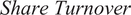
Our model considers three points in time (
 $ {t}_0 $
,
$ {t}_0 $
,
 $ {t}_1 $
, and
$ {t}_1 $
, and
 $ {t}_2 $
), one representative investor, a stock with final payoff
$ {t}_2 $
), one representative investor, a stock with final payoff
 $ {P}_2 $
, and a risk-free investment alternative with a zero return. Figure 1 outlines the sequence of events. In
$ {P}_2 $
, and a risk-free investment alternative with a zero return. Figure 1 outlines the sequence of events. In
 $ {t}_0 $
, the representative investor purchases the stock for an exogenous price of
$ {t}_0 $
, the representative investor purchases the stock for an exogenous price of
 $ {P}_0 $
.Footnote
2 Our arguments do not depend on the specific timing of
$ {P}_0 $
.Footnote
2 Our arguments do not depend on the specific timing of
 $ {t}_0 $
, such that
$ {t}_0 $
, such that
 $ {t}_0 $
might be a few weeks or several years before
$ {t}_0 $
might be a few weeks or several years before
 $ {t}_1 $
. In
$ {t}_1 $
. In
 $ {t}_1 $
, the objective distribution of the final payoff
$ {t}_1 $
, the objective distribution of the final payoff
 $ {P}_2 $
is given by a uniform distribution within the interval
$ {P}_2 $
is given by a uniform distribution within the interval
 $ \left[{E}_1\left({P}_2\right)\pm 0.5\sigma \right] $
with
$ \left[{E}_1\left({P}_2\right)\pm 0.5\sigma \right] $
with
 $ \sigma >0 $
.Footnote
3 This objective payoff distribution reflects all available unbiased information in
$ \sigma >0 $
.Footnote
3 This objective payoff distribution reflects all available unbiased information in
 $ {t}_1 $
, that is, it also reflects potential unbiased information released by the manager in
$ {t}_1 $
, that is, it also reflects potential unbiased information released by the manager in
 $ {t}_1 $
. Beyond this fundamental information, the manager can also communicate a guidance bias
$ {t}_1 $
. Beyond this fundamental information, the manager can also communicate a guidance bias
 $ b $
, that is, in
$ b $
, that is, in
 $ {t}_1 $
, she can state that she expects a final payoff of
$ {t}_1 $
, she can state that she expects a final payoff of
 $ {E}_1\left({P}_2\right)+b $
, though the expected payoff is actually
$ {E}_1\left({P}_2\right)+b $
, though the expected payoff is actually
 $ {E}_1\left({P}_2\right) $
. Finally, payoff uncertainty is resolved in
$ {E}_1\left({P}_2\right) $
. Finally, payoff uncertainty is resolved in
 $ {t}_2 $
and the representative investor receives the payoff
$ {t}_2 $
and the representative investor receives the payoff
 $ {P}_2 $
for each stock she holds.
$ {P}_2 $
for each stock she holds.
Figure 1 outlines the sequence of events in the guidance model. The model incorporates three points in time,
 $ {t}_0 $
,
$ {t}_0 $
,
 $ {t}_1 $
, and
$ {t}_1 $
, and
 $ {t}_2 $
.
$ {t}_2 $
.

1. Investor Beliefs and Investor Utility
Upon receiving the management guidance including the unexpected guidance bias
 $ b $
in
$ b $
in
 $ {t}_1 $
, the investor fully incorporates this information into her beliefs. More specifically, she believes in a payoff distribution that is shifted by
$ {t}_1 $
, the investor fully incorporates this information into her beliefs. More specifically, she believes in a payoff distribution that is shifted by
 $ b $
compared to the rational benchmark such that her updated beliefs imply a uniform distribution of
$ b $
compared to the rational benchmark such that her updated beliefs imply a uniform distribution of
 $ {P}_2 $
in the interval
$ {P}_2 $
in the interval
 $ \left[{E}_1\left({P}_2\right)+b\pm 0.5\sigma \right] $
.Footnote
4 Hence, she does not detect the bias such that she expects a final stock payoff of
$ \left[{E}_1\left({P}_2\right)+b\pm 0.5\sigma \right] $
.Footnote
4 Hence, she does not detect the bias such that she expects a final stock payoff of
 $$ {E}_1^{Inv}\left({P}_2\right)={E}_1\left({P}_2\right)+b, $$
where
 $ {E}_1^{Inv}\left(\cdot \right) $
denotes investor expectations and
$ {E}_1^{Inv}\left(\cdot \right) $
denotes investor expectations and
 $ {E}_1\left(\cdot \right) $
objective expectations, both conditional on the information in
$ {E}_1\left(\cdot \right) $
objective expectations, both conditional on the information in
 $ {t}_1 $
.
$ {t}_1 $
.
The investor’s utility function incorporates two central features: reference point dependence and loss aversion. These two features have been frequently documented and applied in both the asset pricing and corporate finance literature (see, e.g., Shefrin and Statman (Reference Shefrin and Statman1985), Burgstahler and Dichev (Reference Burgstahler and Dichev1997), Degeorge, Patel, and Zeckhauser (Reference Degeorge, Patel and Zeckhauser1999), Graham et al. (Reference Graham, Harvey and Rajgopal2005), Ben-David and Hirshleifer (Reference Ben-David and Hirshleifer2012), An et al. (Reference An, Wang, Wang and Yu2020), and Riley, Summers, and Duxbury (Reference Riley, Summers and Duxbury2020)). More specifically, when evaluating her investment in
 $ {t}_1 $
and
$ {t}_1 $
and
 $ {t}_2 $
, the representative investor uses the stock prices from the previous period (i.e.,
$ {t}_2 $
, the representative investor uses the stock prices from the previous period (i.e.,
 $ {P}_0 $
and
$ {P}_0 $
and
 $ {P}_1 $
, respectively) as reference points. Following Baker et al. (Reference Baker, Mendel and Wurgler2016), we posit that she perceives negative deviations from these reference points as particularly bad. Hence, we scale up the evaluation of losses using a loss aversion parameter of
$ {P}_1 $
, respectively) as reference points. Following Baker et al. (Reference Baker, Mendel and Wurgler2016), we posit that she perceives negative deviations from these reference points as particularly bad. Hence, we scale up the evaluation of losses using a loss aversion parameter of
 $ \left(1+\lambda \right) $
with
$ \left(1+\lambda \right) $
with
 $ \lambda >0 $
. Such an asymmetric evaluation of gains versus losses is well-founded in the psychological literature on loss aversion and a core feature of prospect theory (Kahneman and Tversky (Reference Kahneman and Tversky1979), Tversky and Kahneman (Reference Tversky and Kahneman1992)). For simplicity, we assume linear utility in the gain and loss domain as well as the same utility function in
$ \lambda >0 $
. Such an asymmetric evaluation of gains versus losses is well-founded in the psychological literature on loss aversion and a core feature of prospect theory (Kahneman and Tversky (Reference Kahneman and Tversky1979), Tversky and Kahneman (Reference Tversky and Kahneman1992)). For simplicity, we assume linear utility in the gain and loss domain as well as the same utility function in
 $ {t}_1 $
and
$ {t}_1 $
and
 $ {t}_2 $
. Consequently, the representative investor’s realized utility from holding one stock is given as
$ {t}_2 $
. Consequently, the representative investor’s realized utility from holding one stock is given as
 $$ {u}_1=\left({P}_1-{P}_0\right)\left(1+\lambda {\mathbf{1}}_{P_1<{P}_0}\right)\hskip2em \mathrm{and}\hskip2em {u}_2=\left({P}_2-{P}_1\right)\left(1+\lambda {\mathbf{1}}_{P_2<{P}_1}\right) $$
in
 $ {t}_1 $
and
$ {t}_1 $
and
 $ {t}_2 $
, respectively. This combination of reference point dependence and loss aversion will turn out to be a key determinant for the manager’s choice of guidance bias. Moreover, based on Equation (2), in
$ {t}_2 $
, respectively. This combination of reference point dependence and loss aversion will turn out to be a key determinant for the manager’s choice of guidance bias. Moreover, based on Equation (2), in
 $ {t}_1 $
, the representative investor will allocate her investments between stock and risk-free asset such that she maximizes her expected level of utility
$ {t}_1 $
, the representative investor will allocate her investments between stock and risk-free asset such that she maximizes her expected level of utility
 $ {u}_2 $
, that is,
$ {u}_2 $
, that is,
 $ {E}_1^{Inv}\left({u}_2\right) $
. When trading the stock, the investor is assumed to be a price taker.
$ {E}_1^{Inv}\left({u}_2\right) $
. When trading the stock, the investor is assumed to be a price taker.
2. Manager Utility
We assume that the manager follows an investor perspective such that her utility depends on both
 $ {u}_1 $
and
$ {u}_1 $
and
 $ {u}_2 $
(the investor’s utility from holding the stock from
$ {u}_2 $
(the investor’s utility from holding the stock from
 $ {t}_0 $
to
$ {t}_0 $
to
 $ {t}_1 $
and from
$ {t}_1 $
and from
 $ {t}_1 $
to
$ {t}_1 $
to
 $ {t}_2 $
, respectively). This focus on both intermediate and long-term shareholder value is in line with Leland and Pyle (Reference Leland and Pyle1977), Miller and Rock (Reference Miller and Rock1985), Bebchuk and Stole (Reference Bebchuk and Stole1993), and Baker et al. (Reference Baker, Mendel and Wurgler2016). Moreover, it is motivated by the notion that a poor intermediate investor mood can already have detrimental effects for managers such as reduced compensation and, potentially, CEO turnover. In line with this logic, we assume that the manager cares about the incumbent investor, who can determine managerial compensation and dismissal through their voting rights, instead of the marginal potential investor. Beyond this investor perspective, we assume that the manager suffers personal costs if her forecast from
$ {t}_2 $
, respectively). This focus on both intermediate and long-term shareholder value is in line with Leland and Pyle (Reference Leland and Pyle1977), Miller and Rock (Reference Miller and Rock1985), Bebchuk and Stole (Reference Bebchuk and Stole1993), and Baker et al. (Reference Baker, Mendel and Wurgler2016). Moreover, it is motivated by the notion that a poor intermediate investor mood can already have detrimental effects for managers such as reduced compensation and, potentially, CEO turnover. In line with this logic, we assume that the manager cares about the incumbent investor, who can determine managerial compensation and dismissal through their voting rights, instead of the marginal potential investor. Beyond this investor perspective, we assume that the manager suffers personal costs if her forecast from
 $ {t}_1 $
turns out to be imprecise in
$ {t}_1 $
turns out to be imprecise in
 $ {t}_2 $
. More specifically, we assume that deviations of the final payoff
$ {t}_2 $
. More specifically, we assume that deviations of the final payoff
 $ {P}_2 $
from the provided guidance
$ {P}_2 $
from the provided guidance
 $ {E}_1\left({P}_2\right)+b $
induce costs
$ {E}_1\left({P}_2\right)+b $
induce costs
 $ c $
.Footnote
5 Hence, the manager’s intertemporal utility is given as
$ c $
.Footnote
5 Hence, the manager’s intertemporal utility is given as
 $$ U={u}_1+\beta {u}_2-\beta c\mid {P}_2-\left({E}_1\left({P}_2\right)+b\right)\mid, $$
where
 $ \beta \in \left(0,1\right] $
reflects the manager’s intertemporal utility trade-off between
$ \beta \in \left(0,1\right] $
reflects the manager’s intertemporal utility trade-off between
 $ {t}_1 $
and
$ {t}_1 $
and
 $ {t}_2 $
with lower values of
$ {t}_2 $
with lower values of
 $ \beta $
indicating stronger discounting and a stronger present preference. We assume a rational manager who chooses
$ \beta $
indicating stronger discounting and a stronger present preference. We assume a rational manager who chooses
 $ b $
such that it maximizes her expected level of intertemporal utility
$ b $
such that it maximizes her expected level of intertemporal utility
 $ {E}_1(U) $
. However, the manager’s choice is subject to the plausibility constraint
$ {E}_1(U) $
. However, the manager’s choice is subject to the plausibility constraint
 $ b\in \left[-0.5\sigma, +0.5\sigma \right] $
, that is, we assume that the costs
$ b\in \left[-0.5\sigma, +0.5\sigma \right] $
, that is, we assume that the costs
 $ c $
are sufficiently high such that the manager cannot communicate a payoff forecast for
$ c $
are sufficiently high such that the manager cannot communicate a payoff forecast for
 $ {P}_2 $
that lies outside the range of possible
$ {P}_2 $
that lies outside the range of possible
 $ {P}_2 $
realizations.
$ {P}_2 $
realizations.
B. Model Implications
1. Implications for the Stock Price in
 $ {t}_1 $

In
 $ {t}_1 $
, the investor allocates her funds between stock and risk-free asset such that her expected utility from
$ {t}_1 $
, the investor allocates her funds between stock and risk-free asset such that her expected utility from
 $ {t}_2 $
payoffs is maximized. Hence, in equilibrium, the investor’s marginal expected utility from buying more stocks equals the marginal utility from investing more at the risk-free rate. Given the investor’s loss aversion (Equation (2)), the stock price in
$ {t}_2 $
payoffs is maximized. Hence, in equilibrium, the investor’s marginal expected utility from buying more stocks equals the marginal utility from investing more at the risk-free rate. Given the investor’s loss aversion (Equation (2)), the stock price in
 $ {t}_1 $
equalsFootnote
6
$ {t}_1 $
equalsFootnote
6
 $$ {P}_1={E}_1\left({P}_2\right)+b-\frac{\sigma }{2}+\frac{\sigma }{\lambda}\left(\sqrt{1+\lambda }-1\right). $$
Hence, the stock price depends on rational payoff expectation
 $ {E}_1\left({P}_2\right) $
and guidance bias
$ {E}_1\left({P}_2\right) $
and guidance bias
 $ b $
, where the latter reflects the stock’s temporary mispricing. Such mispricing implications are qualitatively in line with prior catering models that also relax the assumption of market efficiency (Baker and Wurgler (Reference Baker and Wurgler2004), Baker et al. (Reference Baker, Greenwood and Wurgler2009)). The remaining parts of Equation (4) imply
$ b $
, where the latter reflects the stock’s temporary mispricing. Such mispricing implications are qualitatively in line with prior catering models that also relax the assumption of market efficiency (Baker and Wurgler (Reference Baker and Wurgler2004), Baker et al. (Reference Baker, Greenwood and Wurgler2009)). The remaining parts of Equation (4) imply
 $ {P}_1<{E}_1\left({P}_2\right)+b $
such that the investor expects a positive stock return between
$ {P}_1<{E}_1\left({P}_2\right)+b $
such that the investor expects a positive stock return between
 $ {t}_1 $
and
$ {t}_1 $
and
 $ {t}_2 $
. This subjective risk premium compensates the loss-averse investor for payoff risk and increases in
$ {t}_2 $
. This subjective risk premium compensates the loss-averse investor for payoff risk and increases in
 $ \lambda $
, that is, for a given guidance bias
$ \lambda $
, that is, for a given guidance bias
 $ b $
, a higher
$ b $
, a higher
 $ \lambda $
implies a lower stock price. Vice versa, for the limiting case
$ \lambda $
implies a lower stock price. Vice versa, for the limiting case
 $ \lambda \to 0 $
,
$ \lambda \to 0 $
,
 $ {P}_1={E}_1\left({P}_2\right)+b $
, such that the investor expects a return of zero.
$ {P}_1={E}_1\left({P}_2\right)+b $
, such that the investor expects a return of zero.
2. Implications for Management Guidance
Based on Equations (1) to (4), the manager’s expected level of intertemporal utility is given as
 $$ {\displaystyle \begin{array}{c}{E}_1(U)=\left({P}_1^{unbiased}+b-{P}_0\right)\left(1+\lambda {\mathbf{1}}_{P_1^{unbiased}+b<{P}_0}\right)+\beta \left({E}_1\left({P}_2\right)-{P}_1^{unbiased}-b\right)\\ {}-\beta \left(\frac{\lambda }{2\sigma }{\left({P}_1^{unbiased}-{E}_1\left({P}_2\right)+b+\frac{\sigma }{2}\right)}^2+\frac{{c b}^2}{\sigma }+\frac{c\sigma}{4}\right),\end{array}} $$
where
 $ {P}_1^{unbiased} $
is the hypothetical price for the case of unbiased guidance (
$ {P}_1^{unbiased} $
is the hypothetical price for the case of unbiased guidance (
 $ b=0 $
), that is,
$ b=0 $
), that is,
 $ {P}_1^{unbiased}={P}_1-b $
. As evident from Equation (5), the manager’s choice of guidance bias
$ {P}_1^{unbiased}={P}_1-b $
. As evident from Equation (5), the manager’s choice of guidance bias
 $ b $
results from the intertemporal utility trade-off between
$ b $
results from the intertemporal utility trade-off between
 $ {t}_1 $
and
$ {t}_1 $
and
 $ {t}_2 $
. On one hand, providing excessively optimistic forecasts in
$ {t}_2 $
. On one hand, providing excessively optimistic forecasts in
 $ {t}_1 $
increases immediate utility. This positive impact of
$ {t}_1 $
increases immediate utility. This positive impact of
 $ b $
is particularly strong if the stock trades in the investor’s loss domain (i.e., if
$ b $
is particularly strong if the stock trades in the investor’s loss domain (i.e., if
 $ {P}_1={P}_1^{unbiased}+b<{P}_0 $
). On the other hand, raising expectations and thus reference prices in
$ {P}_1={P}_1^{unbiased}+b<{P}_0 $
). On the other hand, raising expectations and thus reference prices in
 $ {t}_1 $
entails three negative effects in
$ {t}_1 $
entails three negative effects in
 $ {t}_2 $
. First, the positive shift in expectations is reversed, implying a utility loss. Second, with respect to the investor’s loss aversion, both the likelihood to incur a loss from
$ {t}_2 $
. First, the positive shift in expectations is reversed, implying a utility loss. Second, with respect to the investor’s loss aversion, both the likelihood to incur a loss from
 $ {t}_1 $
to
$ {t}_1 $
to
 $ {t}_2 $
and the potential loss magnitude linearly increase in
$ {t}_2 $
and the potential loss magnitude linearly increase in
 $ b $
. The combination of these effects results in the first term that is quadratic in
$ b $
. The combination of these effects results in the first term that is quadratic in
 $ b $
. Third, similar arguments imply that expected personal costs are also quadratic in
$ b $
. Third, similar arguments imply that expected personal costs are also quadratic in
 $ b $
as a higher level of
$ b $
as a higher level of
 $ b $
increases both the likelihood of large forecast errors and also the potential magnitude of the corresponding costs (see also the quadratic cost function in Beyer, Guttman, and Marinovic (Reference Beyer, Guttman and Marinovic2019)).
$ b $
increases both the likelihood of large forecast errors and also the potential magnitude of the corresponding costs (see also the quadratic cost function in Beyer, Guttman, and Marinovic (Reference Beyer, Guttman and Marinovic2019)).
A formal investigation of Equation (5) implies that the following guidance bias
 $ {b}^{\ast } $
maximizes the manager’s expected level of intertemporal utility
$ {b}^{\ast } $
maximizes the manager’s expected level of intertemporal utility
 $ {E}_1(U) $
:
$ {E}_1(U) $
:
 $$ {b}^{\ast }=\left\{\begin{array}{llllll}\frac{1-\beta \sqrt{1+\lambda }}{\beta /\sigma (\lambda +2c)}& \mathrm{f}\mathrm{o}\mathrm{r}& & & {P}_0-{P}_1^{unbiased}& <\frac{1-\beta \sqrt{1+\lambda }}{\beta /\sigma (\lambda +2c)}\\ {}{P}_0-{P}_1^{unbiased}& \mathrm{f}\mathrm{o}\mathrm{r}& \frac{1-\beta \sqrt{1+\lambda }}{\beta /\sigma (\lambda +2c)}& \le & {P}_0-{P}_1^{unbiased}& \le \frac{1+\lambda -\beta \sqrt{1+\lambda }}{\beta /\sigma (\lambda +2c)}\\ {}\frac{1+\lambda -\beta \sqrt{1+\lambda }}{\beta /\sigma (\lambda +2c)}& \mathrm{f}\mathrm{o}\mathrm{r}& \frac{1+\lambda -\beta \sqrt{1+\lambda }}{\beta /\sigma (\lambda +2c)}& <& {P}_0-{P}_1^{unbiased}.& \end{array}\right.\operatorname{} $$
The manager is incentivized to issue a guidance bias
 $ {P}_0-{P}_1^{unbiased} $
in order to move
$ {P}_0-{P}_1^{unbiased} $
in order to move
 $ {P}_1 $
toward
$ {P}_1 $
toward
 $ {P}_0 $
, that is, the manager tries to smooth the stock’s price path. More specifically, due to the representative investor’s loss aversion, the manager will try to avoid negative stock returns from
$ {P}_0 $
, that is, the manager tries to smooth the stock’s price path. More specifically, due to the representative investor’s loss aversion, the manager will try to avoid negative stock returns from
 $ {t}_0 $
to
$ {t}_0 $
to
 $ {t}_1 $
. Vice versa, she might also try to avoid and postpone positive returns in order to have some good news in reserve such that the probability for a loss from
$ {t}_1 $
. Vice versa, she might also try to avoid and postpone positive returns in order to have some good news in reserve such that the probability for a loss from
 $ {t}_1 $
to
$ {t}_1 $
to
 $ {t}_2 $
is reduced. However, the manager’s inclination to provide biased forecasts and cater to the investor’s preferences is bound by the costs associated with biased guidance. More specifically, these costs imply that the optimal guidance bias
$ {t}_2 $
is reduced. However, the manager’s inclination to provide biased forecasts and cater to the investor’s preferences is bound by the costs associated with biased guidance. More specifically, these costs imply that the optimal guidance bias
 $ {b}^{\ast } $
always lies between the first optimal solution (lower boundary) and the last optimal solution (upper boundary) shown in Equation (6).
$ {b}^{\ast } $
always lies between the first optimal solution (lower boundary) and the last optimal solution (upper boundary) shown in Equation (6).
According to Equation (6), if both
 $ \lambda =0 $
(no loss aversion) and
$ \lambda =0 $
(no loss aversion) and
 $ \beta =1 $
(no discounting), the manager would not deceive the market (
$ \beta =1 $
(no discounting), the manager would not deceive the market (
 $ {b}^{\ast }=0 $
). Keeping
$ {b}^{\ast }=0 $
). Keeping
 $ \lambda =0 $
, a manager’s discounting (
$ \lambda =0 $
, a manager’s discounting (
 $ \beta <1 $
) implies a positive forecast bias
$ \beta <1 $
) implies a positive forecast bias
 $ {b}^{\ast } $
as the manager prefers immediate over later utility. In particular, without loss aversion,
$ {b}^{\ast } $
as the manager prefers immediate over later utility. In particular, without loss aversion,
 $ {b}^{\ast } $
does not depend on the stock prices
$ {b}^{\ast } $
does not depend on the stock prices
 $ {P}_0 $
and
$ {P}_0 $
and
 $ {P}_1^{unbiased} $
. On the contrary, with
$ {P}_1^{unbiased} $
. On the contrary, with
 $ \lambda >0 $
, the optimal bias
$ \lambda >0 $
, the optimal bias
 $ {b}^{\ast } $
is a function of
$ {b}^{\ast } $
is a function of
 $ {P}_0-{P}_1^{unbiased} $
. This key model prediction also remains qualitatively the same if the manager does not apply any discounting (
$ {P}_0-{P}_1^{unbiased} $
. This key model prediction also remains qualitatively the same if the manager does not apply any discounting (
 $ \beta =1 $
).
$ \beta =1 $
).
The three-part optimal guidance bias
 $ {b}^{\ast } $
from Equation (6) is also depicted in Figure 2. As evident from this figure, our stylized model yields several testable predictions with respect to the optimal guidance bias
$ {b}^{\ast } $
from Equation (6) is also depicted in Figure 2. As evident from this figure, our stylized model yields several testable predictions with respect to the optimal guidance bias
 $ {b}^{\ast } $
. Most importantly,
$ {b}^{\ast } $
. Most importantly,
 $ {b}^{\ast } $
strongly depends on the stock’s previous performance. If the fair value
$ {b}^{\ast } $
strongly depends on the stock’s previous performance. If the fair value
 $ {P}_1^{unbiased} $
implies a loss relative to the purchase price
$ {P}_1^{unbiased} $
implies a loss relative to the purchase price
 $ {P}_0 $
, managers will provide upward-biased forecasts to reduce the magnitude of incurred losses. For stocks in the gain domain, managers might still communicate a positive bias
$ {P}_0 $
, managers will provide upward-biased forecasts to reduce the magnitude of incurred losses. For stocks in the gain domain, managers might still communicate a positive bias
 $ b $
if their present preference is very strong, but might also issue a negative bias to have some good news in reserve. Notwithstanding,
$ b $
if their present preference is very strong, but might also issue a negative bias to have some good news in reserve. Notwithstanding,
 $ b $
will be lower compared to the loss domain because the management does not face strong pressure from discontent investors. These considerations imply our first hypothesis.
$ b $
will be lower compared to the loss domain because the management does not face strong pressure from discontent investors. These considerations imply our first hypothesis.
Hypothesis 1. Management guidance biases decrease in the investors’ return since purchase.
Figure 2 depicts the relationship between the stock’s previous performance (i.e., the hypothetical stock return
 $ {P}_1^{unbiased}/{P}_0-1 $
) and the guidance bias
$ {P}_1^{unbiased}/{P}_0-1 $
) and the guidance bias
 $ {b}^{\ast } $
chosen by the manager to maximize her expected level of intertemporal utility. The baseline scenario uses
$ {b}^{\ast } $
chosen by the manager to maximize her expected level of intertemporal utility. The baseline scenario uses
 $ {P}_0=100 $
as the investor’s initial stock purchase price,
$ {P}_0=100 $
as the investor’s initial stock purchase price,
 $ \lambda =1.25 $
to reflect loss aversion, a discount factor of
$ \lambda =1.25 $
to reflect loss aversion, a discount factor of
 $ \beta =0.75 $
, personal costs for issuing biased forecasts of
$ \beta =0.75 $
, personal costs for issuing biased forecasts of
 $ c=2 $
, and final payoff uncertainty
$ c=2 $
, and final payoff uncertainty
 $ \sigma =40 $
. Beyond this baseline scenario, the “lower
$ \sigma =40 $
. Beyond this baseline scenario, the “lower
 $ \beta $
-scenario” applies
$ \beta $
-scenario” applies
 $ \beta =0.65 $
, the “higher
$ \beta =0.65 $
, the “higher
 $ \sigma $
-scenario” applies
$ \sigma $
-scenario” applies
 $ \sigma =50 $
, and the “lower
$ \sigma =50 $
, and the “lower
 $ c $
-scenario” applies
$ c $
-scenario” applies
 $ c=1 $
.
$ c=1 $
.

In addition to this baseline effect, our model predicts in which situations the relationship between guidance bias and previous stock returns should be particularly strong. For example, a stronger managerial preference for immediate compared to future utility (stronger discounting via lower
 $ \beta $
) carries two implications (see Equation (6) and Figure 2). First, managers will issue more optimistic forecasts to transfer later utility to today. Second, the bias will increase in magnitude as loss aversion and personal cost considerations from
$ \beta $
) carries two implications (see Equation (6) and Figure 2). First, managers will issue more optimistic forecasts to transfer later utility to today. Second, the bias will increase in magnitude as loss aversion and personal cost considerations from
 $ {t}_2 $
play a smaller role.Footnote
7
$ {t}_2 $
play a smaller role.Footnote
7
Hypothesis 2. The negative effect of the investors’ return on guidance biases is stronger when the manager applies stronger discounting.
Further, if the uncertainty with respect to the final payoff is higher (higher
 $ \sigma $
), the magnitude of guidance biases increases. To illustrate this, consider a given positive level of guidance bias
$ \sigma $
), the magnitude of guidance biases increases. To illustrate this, consider a given positive level of guidance bias
 $ b $
. Then, a higher level of
$ b $
. Then, a higher level of
 $ \sigma $
reduces the probability that this positive bias leads to negative stock returns between
$ \sigma $
reduces the probability that this positive bias leads to negative stock returns between
 $ {t}_1 $
and
$ {t}_1 $
and
 $ {t}_2 $
and a corresponding utility loss. Moreover, if
$ {t}_2 $
and a corresponding utility loss. Moreover, if
 $ \sigma $
is high and guidance is imprecise anyway, issuing biased guidance is comparably less costly.
$ \sigma $
is high and guidance is imprecise anyway, issuing biased guidance is comparably less costly.
Hypothesis 3. The negative effect of the investors’ return on guidance biases is stronger if payoff uncertainty is high.
Finally, managers will issue more biased forecasts if the costs
 $ c $
for providing inaccurate estimates are low.
$ c $
for providing inaccurate estimates are low.
Hypothesis 4. The negative effect of the investors’ return on guidance biases is stronger if the manager’s costs for issuing an inaccurate forecast are low.
We empirically examine these four hypotheses in the following.
III. Data
A. Data Sources
We obtain managerial earnings forecasts issued between January 2001 and December 2023 from the IBES Guidance database and only consider U.S. firms with stock listings on NYSE, AMEX, or NASDAQ. We restrict our analysis to annual earnings guidance issued at most 365 days before the associated fiscal year end such that we always focus on the management forecast which is arguably most important for estimating the stock’s fundamental value.Footnote 8 Moreover, we focus on the earliest forecast within this period as management’s level to influence market beliefs and expectations is bigger early within the fiscal year (Rogers and Stocken (Reference Rogers and Stocken2005), Hutton, Lee, and Shu (Reference Hutton, Lee and Shu2012)). Due to our interest in the quantitative accuracy of management forecasts, we require earnings guidance to be sufficiently specific such that we only include point and range estimates. With respect to range estimates, we follow the prior guidance literature and use the midpoint in our analyses (Basi, Carey, and Twark (Reference Basi, Carey and Twark1976), Hassell and Jennings (Reference Hassell and Jennings1986), and Baik et al. (Reference Baik, Farber and Lee2011)). Finally, we follow McNichols (Reference McNichols1989) in excluding stocks with share prices below 10 USD.
Additional stock market, accounting, and analyst data are obtained from CRSP, Compustat, and IBES, respectively. Following Seybert and Yang (Reference Seybert and Yang2012), we use investor sentiment data from the University of Michigan Survey of Consumers. Following Huang et al. (Reference Huang, Ng, Ranasinghe and Zhang2021), we exclude financial firms and utilities due to industry-specific regulations (Standard Industrial Classification (SIC) codes 6000 to 6999 and 4900 to 4949).
B. Variables
1. Dependent Variables
To measure biases in managerial earnings guidance, we define the
 $ Guidance\ Bias $
for fiscal year
$ Guidance\ Bias $
for fiscal year
 $ t $
as the difference between forecasted and realized earnings per share
$ t $
as the difference between forecasted and realized earnings per share
 $ {EPS}_t $
, deflated by the stock price
$ {EPS}_t $
, deflated by the stock price
 $ {P}_{t-1} $
at the beginning of the associated fiscal year (Ajinkya et al. (Reference Ajinkya, Bhojraj and Sengupta2005), Rogers and Stocken (Reference Rogers and Stocken2005), Baik et al. (Reference Baik, Farber and Lee2011)):
$ {P}_{t-1} $
at the beginning of the associated fiscal year (Ajinkya et al. (Reference Ajinkya, Bhojraj and Sengupta2005), Rogers and Stocken (Reference Rogers and Stocken2005), Baik et al. (Reference Baik, Farber and Lee2011)):
 $$ Guidance\hskip0.42em {Bias}_t=\frac{EPS_{forecasted,t}-{EPS}_{realized,t}}{P_{t-1}}\times 100. $$
Hence, the
 $ Guidance $
 $ Bias $
measures which proportion of the firm’s market capitalization is earned more or less than predicted. Positive biases indicate excessively optimistic forecasts, while negative values indicate managerial pessimism relative to the ex post realization.
$ Bias $
measures which proportion of the firm’s market capitalization is earned more or less than predicted. Positive biases indicate excessively optimistic forecasts, while negative values indicate managerial pessimism relative to the ex post realization.
To measure the market’s reaction toward both guidance (announcement of
 $ {EPS}_{forecasted} $
) and actual earnings (announcement of
$ {EPS}_{forecasted} $
) and actual earnings (announcement of
 $ {EPS}_{realized} $
), we calculate cumulative abnormal announcement returns in symmetric 3-day windows around these event dates to determine
$ {EPS}_{realized} $
), we calculate cumulative abnormal announcement returns in symmetric 3-day windows around these event dates to determine
 $ Guidance $
 $ CAR $
and
$ CAR $
and
 $ Earnings $
 $ Announcement $
 $ CAR $
, respectively. Importantly, we focus on the subsequent annual earnings announcement where the earnings, which the guidance refers to, are announced. Abnormal returns are calculated relative to the Fama and French (Reference Fama and French1993) 3-factor model. Following Savor (Reference Savor2012), the underlying factor loadings are estimated using the 255 trading days prior to the event date with a 31-day gap. We require at least 30 valid return observations to estimate factor loadings and event returns.
$ CAR $
, respectively. Importantly, we focus on the subsequent annual earnings announcement where the earnings, which the guidance refers to, are announced. Abnormal returns are calculated relative to the Fama and French (Reference Fama and French1993) 3-factor model. Following Savor (Reference Savor2012), the underlying factor loadings are estimated using the 255 trading days prior to the event date with a 31-day gap. We require at least 30 valid return observations to estimate factor loadings and event returns.
2. Main Explanatory Variable
All explanatory variables are based on firm-level information available at the last turn of month before the management forecast. Annual accounting information is updated each year at the end of June based on the fiscal period that ends in the previous calendar year; this time lag of at least 6 months ensures that the accounting information is publicly available when using it as predictive variable (Fama and French (Reference Fama and French1993)). Since we are interested in the long-run valuation effects of biased forecasts on earnings announcements, we link the later
 $ Earnings $
 $ Announcement $
 $ CAR $
to the same explanatory variable values as the corresponding
$ CAR $
to the same explanatory variable values as the corresponding
 $ Guidance $
 $ CAR $
.
$ CAR $
.
Our model predicts that the
 $ Guidance $
 $ Bias $
depends on the investors’ return since purchase. Therefore, we follow Grinblatt and Han (Reference Grinblatt and Han2005) in estimating the aggregate investor’s purchase price to calculate the capital gains overhang measure
$ Bias $
depends on the investors’ return since purchase. Therefore, we follow Grinblatt and Han (Reference Grinblatt and Han2005) in estimating the aggregate investor’s purchase price to calculate the capital gains overhang measure
 $ CGO $
, which measures the average investor’s stock return since share purchase. Following Grinblatt and Han (Reference Grinblatt and Han2005), the estimation is based on weekly price and trading volume data over the previous 5 years such that the market’s average purchase price in week
$ CGO $
, which measures the average investor’s stock return since share purchase. Following Grinblatt and Han (Reference Grinblatt and Han2005), the estimation is based on weekly price and trading volume data over the previous 5 years such that the market’s average purchase price in week
 $ t $
is given as
$ t $
is given as
 $$ {P}_{pur,t}=\frac{1}{k_t}\sum \limits_{n=1}^{260}\left({Vol}_{t-n}\prod \limits_{\tau =1}^{n-1}\left[1-{Vol}_{t-n+\tau}\right]\right){P}_{t-n}, $$
where
 $ {Vol}_t $
and
$ {Vol}_t $
and
 $ {P}_t $
represent the stock’s turnover ratio and split-adjusted stock price in week
$ {P}_t $
represent the stock’s turnover ratio and split-adjusted stock price in week
 $ t $
, respectively. We truncate the turnover ratios at a maximum level of 1 such that the term in parentheses reflects the proportion of outstanding shares that was purchased for
$ t $
, respectively. We truncate the turnover ratios at a maximum level of 1 such that the term in parentheses reflects the proportion of outstanding shares that was purchased for
 $ {P}_{t-n} $
in week
$ {P}_{t-n} $
in week
 $ t-n $
. We scale the overall sum by the sum of these proportions
$ t-n $
. We scale the overall sum by the sum of these proportions
 $ {k}_t $
such that the 260 weekly weights add up to 1. In order to estimate
$ {k}_t $
such that the 260 weekly weights add up to 1. In order to estimate
 $ {P}_{pur,t} $
, we require at least 100 weekly observations. Based on this aggregate cost basis, we calculate
$ {P}_{pur,t} $
, we require at least 100 weekly observations. Based on this aggregate cost basis, we calculate
 $ CGO $
as
$ CGO $
as
 $$ {CGO}_t=\frac{P_{t-1}-{P}_{pur,t}}{P_{pur,t}}. $$
Our event study uses the last weekly
 $ CGO $
estimate in the month prior to the first guidance announcement. High values of
$ CGO $
estimate in the month prior to the first guidance announcement. High values of
 $ CGO $
indicate that managers face an investor base that is comparably satisfied with the respective stock investment prior to the guidance announcement. The prior empirical literature has emphasized the importance of the purchase price as reference price for investors, the strong influence of
$ CGO $
indicate that managers face an investor base that is comparably satisfied with the respective stock investment prior to the guidance announcement. The prior empirical literature has emphasized the importance of the purchase price as reference price for investors, the strong influence of
 $ CGO $
on the evaluation of their investments, and thus the impact of
$ CGO $
on the evaluation of their investments, and thus the impact of
 $ CGO $
on trading behavior (Shefrin and Statman (Reference Shefrin and Statman1985), Ben-David and Hirshleifer (Reference Ben-David and Hirshleifer2012), An et al. (Reference An, Wang, Wang and Yu2020), and Riley et al. (Reference Riley, Summers and Duxbury2020)).Footnote
9 Thus, even if managers do not tally the purchase price of each investor to compute their respective capital gains, there is strong evidence that
$ CGO $
on trading behavior (Shefrin and Statman (Reference Shefrin and Statman1985), Ben-David and Hirshleifer (Reference Ben-David and Hirshleifer2012), An et al. (Reference An, Wang, Wang and Yu2020), and Riley et al. (Reference Riley, Summers and Duxbury2020)).Footnote
9 Thus, even if managers do not tally the purchase price of each investor to compute their respective capital gains, there is strong evidence that
 $ CGO $
captures investors’ perception of past performance (which managers are likely to perceive and react to).
$ CGO $
captures investors’ perception of past performance (which managers are likely to perceive and react to).
3. Control Explanatory Variables
Our multivariate analyses control for various stock characteristics that have been shown to predict guidance accuracy and guidance biases. For brevity, we shortly introduce these variables in the following, but provide detailed definitions in the Supplementary Material only.
We include the stocks’ market
 $ Beta $
because prior studies show that increased market risk reduces forecast accuracy (Feng et al. (Reference Feng, Li and McVay2009), Baik et al. (Reference Baik, Farber and Lee2011)). Moreover, we control for
$ Beta $
because prior studies show that increased market risk reduces forecast accuracy (Feng et al. (Reference Feng, Li and McVay2009), Baik et al. (Reference Baik, Farber and Lee2011)). Moreover, we control for
 $ Size $
as larger firms have been shown to display a smaller
$ Size $
as larger firms have been shown to display a smaller
 $ Guidance $
 $ Bias $
and a higher forecast accuracy (Ajinkya et al. (Reference Ajinkya, Bhojraj and Sengupta2005)). Similarly, we employ the
$ Bias $
and a higher forecast accuracy (Ajinkya et al. (Reference Ajinkya, Bhojraj and Sengupta2005)). Similarly, we employ the
 $ Book $
-
$ Book $
-
 $ to $
-
$ to $
-
 $ Market $
ratio, which arguably proxies for a firm’s growth opportunities and has been related to forecast properties by the prior literature (Bamber and Cheon (Reference Bamber and Cheon1998), Rogers and Stocken (Reference Rogers and Stocken2005)).
$ Market $
ratio, which arguably proxies for a firm’s growth opportunities and has been related to forecast properties by the prior literature (Bamber and Cheon (Reference Bamber and Cheon1998), Rogers and Stocken (Reference Rogers and Stocken2005)).
Since forecasts made earlier within a given year have been shown to be less accurate and more biased (Ajinkya et al. (Reference Ajinkya, Bhojraj and Sengupta2005), Feng et al. (Reference Feng, Li and McVay2009), Hribar and Yang (Reference Hribar and Yang2016)), we control for the forecast’s time until the period end,
 $ Horizon $
. Further, we include a
$ Horizon $
. Further, we include a
 $ Loss\ Indicator $
based on the firm’s income before extraordinary items as loss firms’ forecasts have been found to be less accurate (Baik et al. (Reference Baik, Farber and Lee2011), Hilary and Hsu (Reference Hilary and Hsu2011)). As Rogers and Stocken (Reference Rogers and Stocken2005) relate industry-specific litigation risk to management guidance, we include a
$ Loss\ Indicator $
based on the firm’s income before extraordinary items as loss firms’ forecasts have been found to be less accurate (Baik et al. (Reference Baik, Farber and Lee2011), Hilary and Hsu (Reference Hilary and Hsu2011)). As Rogers and Stocken (Reference Rogers and Stocken2005) relate industry-specific litigation risk to management guidance, we include a
 $ Process\ Risk $
dummy based on the firm’s SIC code (Cheng and Warfield (Reference Cheng and Warfield2005)). In addition, we control for the
$ Process\ Risk $
dummy based on the firm’s SIC code (Cheng and Warfield (Reference Cheng and Warfield2005)). In addition, we control for the
 $ Prior\ Error $
, which is the one-period lag of
$ Prior\ Error $
, which is the one-period lag of
 $ Guidance\ Bias $
to capture autocorrelation and persistence in guidance biases (set to 0 if missing).
$ Guidance\ Bias $
to capture autocorrelation and persistence in guidance biases (set to 0 if missing).
Furthermore, the broader accounting performance has also been related to guidance properties, prompting us to include Operating Profitability as additional control. Since analyst attention has been shown to constrain management’s willingness to issue inaccurate forecasts (Rogers and Stocken (Reference Rogers and Stocken2005)), we control for the number of analysts (
 $ Analyst\ Coverage $
) and their disagreement (
$ Analyst\ Coverage $
) and their disagreement (
 $ Analyst\ Dispersion $
) calculated according to Johnson (Reference Johnson2004). We also control for the effect of a stock’s return volatility
$ Analyst\ Dispersion $
) calculated according to Johnson (Reference Johnson2004). We also control for the effect of a stock’s return volatility
 $ VOLA $
(see, e.g., Houston, Lev, and Tucker (Reference Houston, Lev and Tucker2010)). Similarly, firms accessing capital markets might be incentivized to issue positively biased guidance (Hribar and Yang (Reference Hribar and Yang2016)), leading us to control for a
$ VOLA $
(see, e.g., Houston, Lev, and Tucker (Reference Houston, Lev and Tucker2010)). Similarly, firms accessing capital markets might be incentivized to issue positively biased guidance (Hribar and Yang (Reference Hribar and Yang2016)), leading us to control for a
 $ Net\; Equity\ Issuer $
dummy variable. Moreover, Bergman and Roychowdhury (Reference Bergman and Roychowdhury2008) illustrate how managers adjust their disclosure strategy to the prevailing investor sentiment, while Seybert and Yang (Reference Seybert and Yang2012) show how sentiment affects
$ Net\; Equity\ Issuer $
dummy variable. Moreover, Bergman and Roychowdhury (Reference Bergman and Roychowdhury2008) illustrate how managers adjust their disclosure strategy to the prevailing investor sentiment, while Seybert and Yang (Reference Seybert and Yang2012) show how sentiment affects
 $ Guidance\; CAR $
. Following these articles, we use the
$ Guidance\; CAR $
. Following these articles, we use the
 $ Investor\ Sentiment $
index from the Michigan Consumer Confidence Index as control.
$ Investor\ Sentiment $
index from the Michigan Consumer Confidence Index as control.
In additional analyses, we use
 $ Share\ Turnover $
and
$ Share\ Turnover $
and
 $ Relative $
 $ Short $
 $ Interest $
, both calculated relative to shares outstanding, as measures of the present preference of guiding managers in our interaction tests. Further, we control for stock returns over different windows prior to the guidance date—Return 1M, Return 3M, Return 1Y, Return 3Y, and Return 5Y—to differentiate between the investors’ average return since purchase (
$ Interest $
, both calculated relative to shares outstanding, as measures of the present preference of guiding managers in our interaction tests. Further, we control for stock returns over different windows prior to the guidance date—Return 1M, Return 3M, Return 1Y, Return 3Y, and Return 5Y—to differentiate between the investors’ average return since purchase (
 $ CGO $
) and the recent stock performance in general. Moreover, we estimate EW CGO, a capital gains overhang measure where we assume identical turnover weights in the cross-section of stocks. More explicitly, for each week
$ CGO $
) and the recent stock performance in general. Moreover, we estimate EW CGO, a capital gains overhang measure where we assume identical turnover weights in the cross-section of stocks. More explicitly, for each week
 $ t $
, we estimate the median weekly stock turnover over the previous 5 years over all common ordinary U.S. stocks. We use this median value as
$ t $
, we estimate the median weekly stock turnover over the previous 5 years over all common ordinary U.S. stocks. We use this median value as
 $ Vol $
in Equation (9). Hence, EW CGO reflects a stock’s past returns with exponentially decaying weights.
$ Vol $
in Equation (9). Hence, EW CGO reflects a stock’s past returns with exponentially decaying weights.
Finally, we control for industry-fixed effects via 2-digit SIC codes in our regressions. All continuous variables are winsorized at the 1% and 99% levels.Footnote
10 Our sample includes all firm-year observations with available data for the three main dependent variables (bias in management guidance as well as cumulative abnormal announcement returns around guidance and earnings announcement dates) and the main independent variable
 $ CGO $
.
$ CGO $
.
C. Summary Statistics
The final sample consists of 14,088 firm-year observations between 2001 and 2023. Descriptive statistics are reported in Table 1. The average earnings forecast exhibits a positive bias of 0.30%. Given the mean market capitalization in our sample, the average guidance bias converts to an overestimation of annual earnings of approximately $33.48 million on average. While the bias conveys that management guidance is, on average, too optimistic, the median bias of −0.09% indicates that the majority of managers tends to underestimate future earnings, which is in line with managerial expectations management aimed at avoiding negative earnings surprises (Matsumoto (Reference Matsumoto2002)) and generating positive earnings surprises (Johnson et al. (Reference Johnson, Kim and So2020)).

Both guidance and earnings announcements are associated with substantial price reactions (see standard deviation of more than 7%). The positive average returns on corporate announcement dates are in line with the empirical evidence of Savor and Wilson (Reference Savor and Wilson2016). On average, investors have experienced a positive stock return of 5.62% since stock purchase prior to the guidance date.
IV. Empirical Evidence on Catering via Earnings Guidance
A. Evidence on the Main Model Prediction
Based on our model, managers might issue pessimistic forecasts if their investors already appreciate the high returns of their investment. In this case, the managers still have positive news in reserve to offset potential unforeseen negative future events which might otherwise have resulted in investor discontent. These arguments are akin to the well-documented expectations management of managers (Ajinkya and Gift (Reference Ajinkya and Gift1984), Johnson et al. (Reference Johnson, Kim and So2020)). On the contrary, we expect managers to issue overly optimistic forecasts when their investors have experienced poor stock returns. In this case, managerial catering could attenuate negative stock performance and, as a consequence, reduce the short-term probability of investor rebellion or CEO turnover (Jenter and Kanaan (Reference Jenter and Kanaan2015)). Thus, we expect
 $ CGO $
to be negatively related to the
$ CGO $
to be negatively related to the
 $ Guidance\ Bias $
as predicted by Hypothesis 1.
$ Guidance\ Bias $
as predicted by Hypothesis 1.
To test our first theoretical prediction, we present results from regression analyses with the
 $ Guidance\ Bias $
as dependent variable in Table 2. While specifications
$ Guidance\ Bias $
as dependent variable in Table 2. While specifications
 $ (1) $
to
$ (1) $
to
 $ (4) $
include industry- and year-fixed effects and control for an increasing number of covariates, specification
$ (4) $
include industry- and year-fixed effects and control for an increasing number of covariates, specification
 $ (5) $
includes firm- and year-fixed effects as well as all applicable control variables. Standard errors are clustered by firm and year across all regressions reported in this article.
$ (5) $
includes firm- and year-fixed effects as well as all applicable control variables. Standard errors are clustered by firm and year across all regressions reported in this article.

In each regression, we find a strong negative relation between
 $ CGO $
and
$ CGO $
and
 $ Guidance $
 $ Bias $
. The statistical significance of the
$ Bias $
. The statistical significance of the
 $ CGO $
coefficient is large across all specifications with t-statistics between −8.31 and −10.76. Similarly, the implied economic magnitude is substantial. Given
$ CGO $
coefficient is large across all specifications with t-statistics between −8.31 and −10.76. Similarly, the implied economic magnitude is substantial. Given
 $ CGO $
coefficients between −1.71 and −2.05, a 1-standard-deviation increase in
$ CGO $
coefficients between −1.71 and −2.05, a 1-standard-deviation increase in
 $ CGO $
is associated with a decrease in
$ CGO $
is associated with a decrease in
 $ Guidance $
 $ Bias $
of 0.26% to 0.31%, which translates to 12.45% to 14.85% of the dependent variable’s standard deviation. Hence, our empirical analysis confirms Hypothesis 1 as lower stock returns of the current investor base go along with more optimistic earnings guidance. Importantly, the effect of
$ Bias $
of 0.26% to 0.31%, which translates to 12.45% to 14.85% of the dependent variable’s standard deviation. Hence, our empirical analysis confirms Hypothesis 1 as lower stock returns of the current investor base go along with more optimistic earnings guidance. Importantly, the effect of
 $ CGO $
is distinct from previously identified determinants of biased guidance.Footnote
11
$ CGO $
is distinct from previously identified determinants of biased guidance.Footnote
11
B. Evidence on Additional Model Predictions
Following our model, the
 $ CGO $
-dependent
$ CGO $
-dependent
 $ Guidance\ Bias $
should be more pronounced when managers have a stronger present preference (Hypothesis 2), the stock’s final payoff is more uncertain (Hypothesis 3), and management’s costs for issuing a deceptive forecast are lower (Hypothesis 4). We apply interaction terms in regression analyses to test whether the effect of
$ Guidance\ Bias $
should be more pronounced when managers have a stronger present preference (Hypothesis 2), the stock’s final payoff is more uncertain (Hypothesis 3), and management’s costs for issuing a deceptive forecast are lower (Hypothesis 4). We apply interaction terms in regression analyses to test whether the effect of
 $ CGO $
on
$ CGO $
on
 $ Guidance\ Bias $
depends on corresponding proxy variables from the prior literature. To allow for simple comparability of effect magnitudes, our regression approach uses dummy variables based on each proxy: if a measure lies above its sample median, we assign a value of 1; otherwise we assign a value of 0. We present the resulting empirical evidence in Table 3.
$ Guidance\ Bias $
depends on corresponding proxy variables from the prior literature. To allow for simple comparability of effect magnitudes, our regression approach uses dummy variables based on each proxy: if a measure lies above its sample median, we assign a value of 1; otherwise we assign a value of 0. We present the resulting empirical evidence in Table 3.

With respect to Hypothesis 2, following Polk and Sapienza (Reference Polk and Sapienza2008) and Bao et al. (Reference Bao, Kim, Mian and Su2019), we argue that the management’s present preference is higher if the firm’s investor base is comparably transient and if the firm faces downward price pressure from short sellers. Hence, we use a stock’s turnover ratio and its relative short interest to measure management’s present preference. Columns
 $ 1 $
and 2 of Table 3 report regression coefficients for the interaction of
$ 1 $
and 2 of Table 3 report regression coefficients for the interaction of
 $ CGO $
with
$ CGO $
with
 $ Share\ Turnover $
and
$ Share\ Turnover $
and
 $ Relative\ Short\ Interest $
dummy, respectively. In both specifications, the interaction effect is significantly negative (at the 1% and 5% levels, respectively). Thus, in line with Hypothesis 2, the effect of
$ Relative\ Short\ Interest $
dummy, respectively. In both specifications, the interaction effect is significantly negative (at the 1% and 5% levels, respectively). Thus, in line with Hypothesis 2, the effect of
 $ CGO $
on
$ CGO $
on
 $ Guidance $
 $ Bias $
becomes stronger if
$ Bias $
becomes stronger if
 $ Share $
 $ Turnover $
and
$ Turnover $
and
 $ Relative\ Short\ Interest $
are large, that is, if managerial myopia is high. Moreover, the interaction terms’ coefficients point toward the high economic magnitude of this mechanism. For example, the impact of
$ Relative\ Short\ Interest $
are large, that is, if managerial myopia is high. Moreover, the interaction terms’ coefficients point toward the high economic magnitude of this mechanism. For example, the impact of
 $ CGO $
on
$ CGO $
on
 $ Guidance\ Bias $
is approximately 2.5 times larger for stocks with high compared to low
$ Guidance\ Bias $
is approximately 2.5 times larger for stocks with high compared to low
 $ Share\ Turnover $
.
$ Share\ Turnover $
.
To measure payoff uncertainty (Hypothesis 3), we consider a firm’s market beta (Beta) and its return volatility (VOLA).Footnote
12 Columns 3 and 4 present the corresponding regression coefficients. Again, both interaction terms predict the
 $ Guidance $
 $ Bias $
with the expected sign and are statistically significant at the 1% level. The effect is also economically meaningful as the effect of
$ Bias $
with the expected sign and are statistically significant at the 1% level. The effect is also economically meaningful as the effect of
 $ CGO $
on
$ CGO $
on
 $ Guidance\ Bias $
increases sharply if either measure lies above its sample median.
$ Guidance\ Bias $
increases sharply if either measure lies above its sample median.
Referring to Hypothesis 4, we argue that the costs of providing inaccurate forecasts should be lower if forecasting is more difficult such that managers can attribute inaccurate forecasts to external factors beyond their control. Columns 5 and 6 of Table 3 examine these arguments by interacting
 $ CGO $
with
$ CGO $
with
 $ Analyst\ Dispersion $
and
$ Analyst\ Dispersion $
and
 $ Horizon $
. The interaction terms of
$ Horizon $
. The interaction terms of
 $ CGO $
with
$ CGO $
with
 $ Analyst\ Dispersion $
and
$ Analyst\ Dispersion $
and
 $ Horizon $
are significantly negative at the 5% level, indicating that managers cater more if analyst disagreement is large and if the forecast is issued comparably early.Footnote
13 Hence, our results support Hypothesis 4.
$ Horizon $
are significantly negative at the 5% level, indicating that managers cater more if analyst disagreement is large and if the forecast is issued comparably early.Footnote
13 Hence, our results support Hypothesis 4.
C. Further Empirical Evidence
1. CGO Versus Past Returns
The prior tests consistently establish that
 $ CGO $
predicts
$ CGO $
predicts
 $ Guidance\ Bias $
as implied by our model. However, one might argue that our regressions just capture correlations between
$ Guidance\ Bias $
as implied by our model. However, one might argue that our regressions just capture correlations between
 $ CGO $
and
$ CGO $
and
 $ Guidance\ Bias $
and thus fail to identify a causal relation between investors’ experienced returns and managerial behavior. It is important to note that we do not claim that managers sit down with a calculator and compute each investor’s rate of return as basis for their guidance strategy. Rather, we theoretically identify
$ Guidance\ Bias $
and thus fail to identify a causal relation between investors’ experienced returns and managerial behavior. It is important to note that we do not claim that managers sit down with a calculator and compute each investor’s rate of return as basis for their guidance strategy. Rather, we theoretically identify
 $ CGO $
as a central determinant of investors’ utility such that it should affect managerial catering because managers should be broadly aware of their investors’ experienced returns. However, one might argue that
$ CGO $
as a central determinant of investors’ utility such that it should affect managerial catering because managers should be broadly aware of their investors’ experienced returns. However, one might argue that
 $ CGO $
also reflects other economic mechanisms since it is closely related to the stock return over the previous 5 years by construction. If this raw return or related measures of firm performance had a direct impact on management guidance, these effects might be captured by
$ CGO $
also reflects other economic mechanisms since it is closely related to the stock return over the previous 5 years by construction. If this raw return or related measures of firm performance had a direct impact on management guidance, these effects might be captured by
 $ CGO $
. We therefore add the firm’s stock returns over several event windows prior to the guidance date—1 month, 3 months, 1 year, 3 years, and 5 years—as control variables. While these return variables should capture general arguments related to firm performance, the remaining effect associated with
$ CGO $
. We therefore add the firm’s stock returns over several event windows prior to the guidance date—1 month, 3 months, 1 year, 3 years, and 5 years—as control variables. While these return variables should capture general arguments related to firm performance, the remaining effect associated with
 $ CGO $
exhibits a clear connection to investors’ experienced returns since
$ CGO $
exhibits a clear connection to investors’ experienced returns since
 $ CGO $
reflects the turnover-weighted returns of the previous 5 years.
$ CGO $
reflects the turnover-weighted returns of the previous 5 years.
Table 4 reports regression results of Guidance Bias on
 $ CGO $
and the five different return variables separately in columns 1 to 5 and jointly in column 6. Notably, CGO remains statistically significant at the 1% level and economically large (coefficients between −1.11 and −1.89) across all specifications. One of the five return variables (Return 1Y) is also significantly related to Guidance Bias, yet does not lead to a loss of significance in the CGO–Guidance Bias relation. These results emphasize that managers are clearly more responsive to the returns experienced by investors than the overall return over the past years, which provides further evidence for the proposed catering channel.Footnote
14
$ CGO $
and the five different return variables separately in columns 1 to 5 and jointly in column 6. Notably, CGO remains statistically significant at the 1% level and economically large (coefficients between −1.11 and −1.89) across all specifications. One of the five return variables (Return 1Y) is also significantly related to Guidance Bias, yet does not lead to a loss of significance in the CGO–Guidance Bias relation. These results emphasize that managers are clearly more responsive to the returns experienced by investors than the overall return over the past years, which provides further evidence for the proposed catering channel.Footnote
14

Finally, we insert EW CGO alongside CGO in column 7 of Table 4. This specification constitutes a particularly demanding test of the catering theory of earnings guidance: EW CGO is also computed based on weekly stock returns over the preceding 260 weeks, yet these returns are weighted with market-wide median (instead of firm-specific) turnover. Consequently, EW CGO captures all arguments related to weighted past returns. Hence, the remaining effect of CGO essentially stems from firms with the same past returns but different investor capital gains that we infer from different purchase dates based on the different turnover dynamics. Controlling for EW CGO—which exhibits a correlation with CGO of 80.50%—reduces the CGO coefficient to −0.76. Nonetheless, the effect of CGO remains both statistically significant at the 1% level and economically large.
2. Catering Versus Biased Beliefs
As alternative underlying mechanism, the documented effect of
 $ CGO $
on
$ CGO $
on
 $ Guidance\ Bias $
might also reflect a systematic managerial bias akin to the investor bias associated with
$ Guidance\ Bias $
might also reflect a systematic managerial bias akin to the investor bias associated with
 $ CGO $
(Grinblatt and Han (Reference Grinblatt and Han2005)). In addition, the managers’ own beliefs might be excessively optimistic if
$ CGO $
(Grinblatt and Han (Reference Grinblatt and Han2005)). In addition, the managers’ own beliefs might be excessively optimistic if
 $ CGO $
is low such that our key findings might reflect managers’ judgment biases rather than catering. However, this alternative line of argument is difficult to reconcile with the interaction tests in Table 3 that support the more nuanced catering implications of our model. To further bolster the evidence for intentional managerial catering, we explicitly address three channels through which managerial biases could be tied to
$ CGO $
is low such that our key findings might reflect managers’ judgment biases rather than catering. However, this alternative line of argument is difficult to reconcile with the interaction tests in Table 3 that support the more nuanced catering implications of our model. To further bolster the evidence for intentional managerial catering, we explicitly address three channels through which managerial biases could be tied to
 $ CGO $
:
$ CGO $
:
i) Biases in beliefs are frequently associated with high levels of sentiment (Seybert and Yang (Reference Seybert and Yang2012), Stambaugh, Yu, and Yuan (Reference Stambaugh, Yu and Yuan2012)). If biased managerial beliefs caused the effect of
 $ CGO $
on Guidance Bias, we would expect it to intensify substantially in times of high investor sentiment. Interaction tests in our Supplementary Material show that the CGO effect does not depend strongly on sentiment and remains economically large in times of low sentiment.
$ CGO $
on Guidance Bias, we would expect it to intensify substantially in times of high investor sentiment. Interaction tests in our Supplementary Material show that the CGO effect does not depend strongly on sentiment and remains economically large in times of low sentiment.
ii) Overconfidence is a frequently studied distortion of managerial beliefs (see, e.g., Malmendier and Tate (Reference Malmendier and Tate2005), (Reference Malmendier and Tate2008)). Such overconfidence might manifest in excessively optimistic earnings forecasts after poor stock returns because managers disregard the cause of the stock price decline or overestimate their ability to address it. Then, the effect of
 $ CGO $
on Guidance Bias should be particularly strong for overconfident managers. In fact, we show in our Supplementary Material that the effect of
$ CGO $
on Guidance Bias should be particularly strong for overconfident managers. In fact, we show in our Supplementary Material that the effect of
 $ CGO $
on earnings guidance is—if anything—smaller for overconfident managers. This result indicates that biased managerial beliefs constrain
$ CGO $
on earnings guidance is—if anything—smaller for overconfident managers. This result indicates that biased managerial beliefs constrain
 $ CGO $
-dependent catering (instead of causing it).
$ CGO $
-dependent catering (instead of causing it).
iii) The effect of
 $ CGO $
on earnings guidance could emerge because
$ CGO $
on earnings guidance could emerge because
 $ CGO $
might also reflect the manager’s capital gains, which in turn could relate to her beliefs—for example, due to motivated reasoning (Zimmermann (Reference Zimmermann2020)). We document in our Supplementary Material that the effect of
$ CGO $
might also reflect the manager’s capital gains, which in turn could relate to her beliefs—for example, due to motivated reasoning (Zimmermann (Reference Zimmermann2020)). We document in our Supplementary Material that the effect of
 $ CGO $
is unaffected by the inclusion of the CEO’s equity share as interaction term.Footnote
15 This finding is at odds with the assumption that managerial capital gains drive the
$ CGO $
is unaffected by the inclusion of the CEO’s equity share as interaction term.Footnote
15 This finding is at odds with the assumption that managerial capital gains drive the
 $ CGO $
effect as even managers without equity share engage in catering. Overall, our results support the notion that intentional managerial catering is the source of the
$ CGO $
effect as even managers without equity share engage in catering. Overall, our results support the notion that intentional managerial catering is the source of the
 $ CGO $
effect in earnings guidance.
$ CGO $
effect in earnings guidance.
3. Further Robustness Tests
We provide a number of further robustness tests in the Supplementary Material. In particular, we document that the effect of
 $ CGO $
on
$ CGO $
on
 $ Guidance\ Bias $
is economically large and of comparable magnitude for point and range forecasts based on subsample tests. Additionally, we document that the CGO–Guidance Bias relation is large irrespective of the share of institutional ownership. Moreover, our findings could be related to Baginski et al. (Reference Baginski, Campbell, Ryu and Warren2023) who document that a positive (negative)
$ Guidance\ Bias $
is economically large and of comparable magnitude for point and range forecasts based on subsample tests. Additionally, we document that the CGO–Guidance Bias relation is large irrespective of the share of institutional ownership. Moreover, our findings could be related to Baginski et al. (Reference Baginski, Campbell, Ryu and Warren2023) who document that a positive (negative)
 $ Guidance\ Bias $
is associated with negative (positive) earnings surprises revealed at concurrent earnings announcements. We do not control for earnings surprises in our prior analyses because our sample also includes guidance announcements without concurrent earnings announcements. All results presented in this article, however, remain qualitatively unchanged if we limit our sample to guidance announcements with concurrent earnings announcements and control for earnings surprises. We report two central pieces of evidence in our Supplementary Material: i) We show that the effect of
$ Guidance\ Bias $
is associated with negative (positive) earnings surprises revealed at concurrent earnings announcements. We do not control for earnings surprises in our prior analyses because our sample also includes guidance announcements without concurrent earnings announcements. All results presented in this article, however, remain qualitatively unchanged if we limit our sample to guidance announcements with concurrent earnings announcements and control for earnings surprises. We report two central pieces of evidence in our Supplementary Material: i) We show that the effect of
 $ CGO $
on
$ CGO $
on
 $ Guidance\ Bias $
remains significant in the subsample of guidance announcements without concurrent earnings announcements. ii) Controlling for earnings surprises does not change the effect of
$ Guidance\ Bias $
remains significant in the subsample of guidance announcements without concurrent earnings announcements. ii) Controlling for earnings surprises does not change the effect of
 $ CGO $
on
$ CGO $
on
 $ Guidance\ Bias $
.
$ Guidance\ Bias $
.
Figure 2 implies that the effect of the investor’s past returns is large for moderate values of past returns and flattens out for extreme positive and negative values. We provide two pieces of empirical evidence, which are consistent with such a reduced sensitivity toward extreme returns. i) Escalating the levels of CGO winsorization increases the negative effect of CGO on Guidance Bias. ii) Interacting CGO with a dummy variable, which is equal to 1 if the absolute value of CGO is smaller than 10%, and 0 otherwise, confirms that the effect is strongest for moderate CGO values.
Finally, our catering theory rests on the assumption that discontented investors exert pressure on the manager such that the manager’s intertemporal utility depends on both short-term and long-term firm performance. We argue that CEOs might be particularly inclined to engage in
 $ CGO $
-dependent catering if the stock performance reflected by
$ CGO $
-dependent catering if the stock performance reflected by
 $ CGO $
can be attributed to them. In this case, the link between investor and manager utility should be stronger because, for example, investors’ utility losses might result in investor rebellion and CEO dismissal. Analyses based on recently employed CEOs confirm that the effect is driven by established managers and insignificant for newly appointed managers.
$ CGO $
can be attributed to them. In this case, the link between investor and manager utility should be stronger because, for example, investors’ utility losses might result in investor rebellion and CEO dismissal. Analyses based on recently employed CEOs confirm that the effect is driven by established managers and insignificant for newly appointed managers.
4. Ex Post Consequences of Catering
CEO-Specific Consequences of Catering. Our theoretical model predicts that Guidance Bias depends on CGO because managers respond to investors’ reference point-dependent loss aversion. The prior empirical evidence strongly supports this proposition, while also pointing toward substantial heterogeneity in this propensity to cater. In addition to the stock market consequences, which we examine in Section V, this also raises the question, whether catering via earnings guidance has any implications for CEOs’ careers. In line with the intuition laid out in our theoretical model, we conjecture that CEOs’ responsiveness to the investor mood is advantageous for them.
We test this hypothesis by identifying CEOs whose biases in forecasts are consistent with catering, that is, they tend to issue excessively optimistic (pessimistic) guidance when investors are in their loss (gain) domain. We provide two pieces of evidence in our Supplementary Material that suggest that these CEOs are indeed better off. First, comparing average career outcomes, we find that catering CEOs are associated with higher total compensation—in particular driven by incentive-based pay—and longer tenures. Second, we examine the annual likelihood of CEO turnover, CEO dismissal, and total compensation in a firm-year panel. The results confirm that catering CEOs are less likely to be replaced and receive higher compensation.Footnote 16 These results suggest that catering via earnings guidance pays off for CEOs.
Firm-Specific Consequences of Catering. Earnings guidance is a particularly well-suited laboratory to test theories of managerial catering, given the comparably low personal costs for managers if forecasts do not materialize exactly as predicted. Whether such catering via earnings guidance coincides with other forms of misstatement is an empirical question, which we test using the Dechow et al. (Reference Dechow, Ge, Larson and Sloan2011) dataset on material accounting misstatements. We conjecture that managers of low-CGO firms might not only publish too optimistic earnings guidance, but might also have the strongest incentives to publish incorrect accounting figures. In line with this conjecture, our Supplementary Material shows that catering goes along with a negative relationship between CGO and the likelihood of a concurrent misstatement of financial accounting data. We interpret this as initial evidence that the incentives that cause firms to cater via earnings guidance might also affect other, more costly forms of biased disclosure.Footnote 17 Consequently, this result points toward the wider implications of investors’ reference point-dependent loss aversion for corporate policies.
V. Stock Market Implications
In this section, we examine the stock market implications of
 $ CGO $
-dependent managerial catering. More specifically, we employ both non-parametric portfolio sorts and multivariate regression analyses to test whether catering succeeds in moving market prices.
$ CGO $
-dependent managerial catering. More specifically, we employ both non-parametric portfolio sorts and multivariate regression analyses to test whether catering succeeds in moving market prices.
A. Univariate Evidence
As a first step, we conduct cross-sectional quintile portfolio sorts based on
 $ CGO $
. More precisely, for each month in our sample, we define portfolio breakpoints based on
$ CGO $
. More precisely, for each month in our sample, we define portfolio breakpoints based on
 $ CGO $
using all common ordinary U.S. stocks trading on NYSE, AMEX, or NASDAQ. Based on these breakpoints, each observation is assigned to one of five portfolios based on
$ CGO $
using all common ordinary U.S. stocks trading on NYSE, AMEX, or NASDAQ. Based on these breakpoints, each observation is assigned to one of five portfolios based on
 $ CGO $
. Consequently, also non-guiding firms are considered for portfolio construction, while our reported figures naturally focus on guiding firms. We follow Seybert and Yang (Reference Seybert and Yang2012) in adopting a purely cross-sectional approach for two reasons. First, investors usually judge their investment performance relative to other stocks at a given point in time such that the cross-sectional positioning of a stock should be relevant for managers’ catering decisions. Second, we do not want nearly all observations in a given month to be allocated to the top (bottom) portfolio simply because the overall market has substantially increased (decreased) in the recent past. Nonetheless, the Supplementary Material reports qualitatively the same results if we pool all observations from our sample to form portfolios.
$ CGO $
. Consequently, also non-guiding firms are considered for portfolio construction, while our reported figures naturally focus on guiding firms. We follow Seybert and Yang (Reference Seybert and Yang2012) in adopting a purely cross-sectional approach for two reasons. First, investors usually judge their investment performance relative to other stocks at a given point in time such that the cross-sectional positioning of a stock should be relevant for managers’ catering decisions. Second, we do not want nearly all observations in a given month to be allocated to the top (bottom) portfolio simply because the overall market has substantially increased (decreased) in the recent past. Nonetheless, the Supplementary Material reports qualitatively the same results if we pool all observations from our sample to form portfolios.
The average
 $ Guidance $
 $ Bias $
for each
$ Bias $
for each
 $ CGO $
quintile portfolio is presented in Figure 3. The blue bars show that the
$ CGO $
quintile portfolio is presented in Figure 3. The blue bars show that the
 $ Guidance $
 $ Bias $
decreases across the five
$ Bias $
decreases across the five
 $ CGO $
quintiles. While low-
$ CGO $
quintiles. While low-
 $ CGO $
firms exhibit the largest average bias of 1.16%, managers of high-
$ CGO $
firms exhibit the largest average bias of 1.16%, managers of high-
 $ CGO $
firms issue forecasts with a negative bias of −0.03% on average. Thus, Figure 3 supports our results from Section IV on the negative relationship between
$ CGO $
firms issue forecasts with a negative bias of −0.03% on average. Thus, Figure 3 supports our results from Section IV on the negative relationship between
 $ CGO $
and
$ CGO $
and
 $ Guidance $
 $ Bias $
, yielding additional nonparametric support for Hypothesis 1. Moreover, Figure 3 confirms our model prediction that catering is particularly strong among low-
$ Bias $
, yielding additional nonparametric support for Hypothesis 1. Moreover, Figure 3 confirms our model prediction that catering is particularly strong among low-
 $ CGO $
firms. First, these forecasts are prone to the largest bias in absolute magnitude. Second, even after subtracting managers’ overall tendency to predict too high earnings (0.30%, see Table 1), the magnitude of
$ CGO $
firms. First, these forecasts are prone to the largest bias in absolute magnitude. Second, even after subtracting managers’ overall tendency to predict too high earnings (0.30%, see Table 1), the magnitude of
 $ Guidance $
 $ Bias $
is more pronounced for low-
$ Bias $
is more pronounced for low-
 $ CGO $
compared to high-
$ CGO $
compared to high-
 $ CGO $
firms. These observations are in line with investors’ loss aversion and managers’ present preference that predict the strongest effects among firms with low
$ CGO $
firms. These observations are in line with investors’ loss aversion and managers’ present preference that predict the strongest effects among firms with low
 $ CGO $
(see Figure 2).
$ CGO $
(see Figure 2).
Figure 3 depicts cross-sectional portfolio sorts based on
 $ CGO $
for the sample period from 2001 to 2023. In each month, stocks are allocated to quintile portfolios using breakpoints based on the entire cross-section of U.S. stocks. For each portfolio, the figure presents the average
$ CGO $
for the sample period from 2001 to 2023. In each month, stocks are allocated to quintile portfolios using breakpoints based on the entire cross-section of U.S. stocks. For each portfolio, the figure presents the average
 $ Guidance $
 $ Bias $
(blue bars), defined as the difference between forecasted EPS and realized EPS, divided by the stock price at the beginning of the fiscal year. In addition, it depicts the abnormal stock returns around the corresponding management guidance (red bars). These abnormal returns are calculated for a symmetric 3-day window around the announcement date relative to the Fama and French (Reference Fama and French1993) 3-factor model where the underlying factor loadings are estimated using the 255 trading days prior to the event date with a 31-day gap.
$ Bias $
(blue bars), defined as the difference between forecasted EPS and realized EPS, divided by the stock price at the beginning of the fiscal year. In addition, it depicts the abnormal stock returns around the corresponding management guidance (red bars). These abnormal returns are calculated for a symmetric 3-day window around the announcement date relative to the Fama and French (Reference Fama and French1993) 3-factor model where the underlying factor loadings are estimated using the 255 trading days prior to the event date with a 31-day gap.

If the stock market does not acknowledge managers’ incentives to provide systematically biased guidance, we expect catering to succeed in influencing short-term stock prices. Therefore, firms with relatively low
 $ CGO $
values should experience relatively high
$ CGO $
values should experience relatively high
 $ Guidance $
 $ CAR $
and vice versa. The red bars in Figure 3 support this conjecture: the average abnormal returns around guidance dates decrease sharply from 1.59% for low-
$ CAR $
and vice versa. The red bars in Figure 3 support this conjecture: the average abnormal returns around guidance dates decrease sharply from 1.59% for low-
 $ CGO $
firms to 0.37% for high-
$ CGO $
firms to 0.37% for high-
 $ CGO $
firms. In conclusion, Figure 3 shows that the
$ CGO $
firms. In conclusion, Figure 3 shows that the
 $ Guidance $
 $ CAR $
declines as
$ CAR $
declines as
 $ CGO $
increases.
$ CGO $
increases.
Table 5 tests the statistical significance to the graphical evidence from Figure 3. The difference in
 $ Guidance $
 $ Bias $
between high- versus low-
$ Bias $
between high- versus low-
 $ CGO $
firms is highly significant and the spread of −1.20% is also economically large as it equals 57.48% of the
$ CGO $
firms is highly significant and the spread of −1.20% is also economically large as it equals 57.48% of the
 $ Guidance $
 $ Bias $
standard deviation. Moreover, low-
$ Bias $
standard deviation. Moreover, low-
 $ CGO $
firms’
$ CGO $
firms’
 $ Guidance $
 $ CAR $
exceed high-
$ CAR $
exceed high-
 $ CGO $
firms’
$ CGO $
firms’
 $ Guidance $
 $ CAR $
by 1.21% (significant at the 5% level). Hence, the market reaction suggests that investors do not fully appreciate the systematic effect of
$ CAR $
by 1.21% (significant at the 5% level). Hence, the market reaction suggests that investors do not fully appreciate the systematic effect of
 $ CGO $
on
$ CGO $
on
 $ Guidance $
 $ Bias $
.
$ Bias $
.

The number of observations per quintile reported in Table 5 indicates that there is also an effect of the investors’ return since purchase on the decision to guide: low-
 $ CGO $
firms are less likely to provide earnings guidance. Importantly, our main results remain qualitatively unchanged if we restrict the sample to firms which also issued an earnings forecast in the previous year.
$ CGO $
firms are less likely to provide earnings guidance. Importantly, our main results remain qualitatively unchanged if we restrict the sample to firms which also issued an earnings forecast in the previous year.
As managerial catering seems to convey erroneous earnings expectations to the market, thereby inducing systematic stock mispricing, we also examine the resolution of this mispricing. We argue that those managers, who have the strongest incentives to cater, are also the least likely to correct mispricing themselves due to the potentially adverse impact on their investors’ attitude toward the firm. Our Supplementary Material confirms that even the last guidance issued before the final earnings announcement is prone to a strong
 $ CGO $
-dependent
$ CGO $
-dependent
 $ Guidance\ Bias $
. Hence, the forecast biases should be partially corrected when the actual earnings are announced. Thus, we expect that low-
$ Guidance\ Bias $
. Hence, the forecast biases should be partially corrected when the actual earnings are announced. Thus, we expect that low-
 $ CGO $
firms experience lower
$ CGO $
firms experience lower
 $ Earnings $
 $ Announcement $
 $ CAR $
than high-
$ CAR $
than high-
 $ CGO $
firms. The third row in Table 5 supports this hypothesis: high-
$ CGO $
firms. The third row in Table 5 supports this hypothesis: high-
 $ CGO $
firms, which have previously understated future earnings on average, experience significantly positive
$ CGO $
firms, which have previously understated future earnings on average, experience significantly positive
 $ Earnings $
 $ Announcement $
 $ CAR $
of 0.75%. Conversely, low-
$ CAR $
of 0.75%. Conversely, low-
 $ CGO $
firms, which issued excessively optimistic forecasts and experienced high
$ CGO $
firms, which issued excessively optimistic forecasts and experienced high
 $ Guidance $
 $ CAR $
on average, yield low earnings announcement returns of −0.21%. Thus, low-
$ CAR $
on average, yield low earnings announcement returns of −0.21%. Thus, low-
 $ CGO $
firms exhibit
$ CGO $
firms exhibit
 $ Earnings $
 $ Announcement $
 $ CAR $
far below the sample mean of 0.35% (see Table 1). The 0.96% difference between high- and low-
$ CAR $
far below the sample mean of 0.35% (see Table 1). The 0.96% difference between high- and low-
 $ CGO $
firms is statistically significant at the 1% level, lending support to our hypothesis that the mispricing induced by managerial catering is at least partially corrected when the actual earnings are announced.
$ CGO $
firms is statistically significant at the 1% level, lending support to our hypothesis that the mispricing induced by managerial catering is at least partially corrected when the actual earnings are announced.
In summary, our univariate analyses show that managers of low-
 $ CGO $
firms issue excessively optimistic earnings guidance, which is associated with a strong positive initial market reaction as well as subpar market reception to the subsequent earnings announcement.
$ CGO $
firms issue excessively optimistic earnings guidance, which is associated with a strong positive initial market reaction as well as subpar market reception to the subsequent earnings announcement.
B. Multivariate Evidence
To delve deeper into the stock price implications of catering, we examine cumulative abnormal returns around guidance and subsequent earnings announcement dates based on multivariate regressions. Table 6 shows regression analyses with
 $ Guidance\ CAR $
as dependent variable in columns 1–3 and
$ Guidance\ CAR $
as dependent variable in columns 1–3 and
 $ Earnings\ Announcement\ CAR $
in columns 4–6. We employ the same set of control variables used to explain
$ Earnings\ Announcement\ CAR $
in columns 4–6. We employ the same set of control variables used to explain
 $ Guidance\ Bias $
in Table 2.
$ Guidance\ Bias $
in Table 2.

In line with the univariate evidence from the previous subsection, columns 1 to 3 show that
 $ CGO $
-dependent managerial catering seemingly succeeds in moving market participants’ earnings expectations and, as a consequence, stock market prices in the short run. In particular, the effect remains highly significant after taking the predictive power of the control variables into account. Columns 4 to 6 of Table 6 report results of regressions with
$ CGO $
-dependent managerial catering seemingly succeeds in moving market participants’ earnings expectations and, as a consequence, stock market prices in the short run. In particular, the effect remains highly significant after taking the predictive power of the control variables into account. Columns 4 to 6 of Table 6 report results of regressions with
 $ Earnings $
 $ Announcement $
 $ CAR $
as dependent variable. The
$ CAR $
as dependent variable. The
 $ CGO $
coefficient is significantly positive across all specifications. Therefore, a substantial portion of the initial
$ CGO $
coefficient is significantly positive across all specifications. Therefore, a substantial portion of the initial
 $ CGO $
-dependent guidance announcement return is reversed around the subsequent annual earnings announcement date. Taken together with Table 5, these findings indicate that the systematic effect of
$ CGO $
-dependent guidance announcement return is reversed around the subsequent annual earnings announcement date. Taken together with Table 5, these findings indicate that the systematic effect of
 $ CGO $
on
$ CGO $
on
 $ Guidance $
 $ Bias $
fuels an overvaluation of low-
$ Bias $
fuels an overvaluation of low-
 $ CGO $
firms, which is largely alleviated around the earnings announcements, where true earnings are announced.
$ CGO $
firms, which is largely alleviated around the earnings announcements, where true earnings are announced.
We conduct three additional tests of the stock market implications of catering via earnings guidance, which we report in the Supplementary Material. First, applying a two-stage least squares regression procedure, we find that the portion of
 $ Guidance\ Bias $
predicted by pre-guidance
$ Guidance\ Bias $
predicted by pre-guidance
 $ CGO $
has a significantly positive impact on
$ CGO $
has a significantly positive impact on
 $ Guidance\; CAR $
and a significantly negative impact on
$ Guidance\; CAR $
and a significantly negative impact on
 $ Earnings\ Announcement\; CAR $
. Second, we study whether the price impact of catering via earnings guidance reverses at intermediate quarterly earnings announcements, that is, quarterly earnings announcements after the initial guidance date and before the final annual earnings announcement. We do not find any evidence of a systematic reversal at these intermediate quarterly earnings announcements, which is consistent with the notion that a large portion of the investor’s biased earnings expectations is corrected when the true final earnings are revealed. Third, we examine the relation between CGO and Earnings Announcement CAR for a matched sample of non-guiding firms. For these non-guiding firms, CGO is no significant return predictor suggesting that the positive effect of CGO on Earnings Announcement CAR in our main sample is indeed driven by catering via earnings guidance.
$ Earnings\ Announcement\; CAR $
. Second, we study whether the price impact of catering via earnings guidance reverses at intermediate quarterly earnings announcements, that is, quarterly earnings announcements after the initial guidance date and before the final annual earnings announcement. We do not find any evidence of a systematic reversal at these intermediate quarterly earnings announcements, which is consistent with the notion that a large portion of the investor’s biased earnings expectations is corrected when the true final earnings are revealed. Third, we examine the relation between CGO and Earnings Announcement CAR for a matched sample of non-guiding firms. For these non-guiding firms, CGO is no significant return predictor suggesting that the positive effect of CGO on Earnings Announcement CAR in our main sample is indeed driven by catering via earnings guidance.
VI. CGO and Analyst Expectations
Section II implies that managers cater to reference point-dependent loss-averse investor preferences through systematically biased guidance. Hence, market participants should be overly optimistic with respect to the earnings of low-CGO firms. We test this proposition by compiling a sample of aggregate analyst expectations from the monthly IBES summary file and applying equivalent filters to our guidance sample.Footnote 18 Then, we define Analyst Bias analogously to Guidance Bias by taking the difference of the median EPS forecasts of analysts and the ex post EPS realization, deflated by the stock price at the beginning of the fiscal year (in %). We regress Analyst Bias on CGO and report the resulting coefficients in Table 7.

Table 7 confirms that CGO is significantly negatively related to Analyst Bias. The economic effect is also sizable, though attenuated compared to the CGO effect on Guidance Bias (see Table 2): focusing on the most comprehensive specification, a 1-standard-deviation increase in CGO reduces Analyst Bias by 11.39% and Guidance Bias by 14.29% of their respective standard deviations. These results—in particular in conjunction with Table 6—are consistent with CGO-dependent catering shaping the beliefs of stock market participants.Footnote 19
VII. Conclusion
In this article, we propose a catering theory of earnings guidance. Our theory implies that managers cater to loss-averse investors by issuing excessively optimistic forecasts when investors have experienced disappointing stock returns. Both regression evidence and univariate analyses support this conjecture. Consistent with managerial catering, the relation between
 $ CGO $
, the average investor’s return since stock purchase, and
$ CGO $
, the average investor’s return since stock purchase, and
 $ Guidance\ Bias $
is particularly strong if managers are myopic, face low personal costs for issuing biased forecasts, and if their firm’s stock return is volatile. Moreover, the negative effect of
$ Guidance\ Bias $
is particularly strong if managers are myopic, face low personal costs for issuing biased forecasts, and if their firm’s stock return is volatile. Moreover, the negative effect of
 $ CGO $
on
$ CGO $
on
 $ Guidance\ Bias $
is distinct from the effect of past returns.
$ Guidance\ Bias $
is distinct from the effect of past returns.
We also find that low-
 $ CGO $
firms experience significantly higher returns than high-
$ CGO $
firms experience significantly higher returns than high-
 $ CGO $
firms around guidance announcements. This empirical observation suggests that biased forecasts succeed in moving market prices in the short run, though the return effects reverse upon the final earnings announcements. Consequently, while accounting regulation has substantially reduced leeway in earnings management, managers successfully use earnings forecasts for catering instead. Thus, in order to constrain opportunistic motives in voluntary guidance and mitigate the resulting distortions of stock prices, our theoretical and empirical evidence provides additional arguments for strict governance and potentially even further regulation beyond the SEC’s “Regulation Fair Disclosure.” Moreover, market participants should carefully take managerial motives into account when processing corresponding firm information.
$ CGO $
firms around guidance announcements. This empirical observation suggests that biased forecasts succeed in moving market prices in the short run, though the return effects reverse upon the final earnings announcements. Consequently, while accounting regulation has substantially reduced leeway in earnings management, managers successfully use earnings forecasts for catering instead. Thus, in order to constrain opportunistic motives in voluntary guidance and mitigate the resulting distortions of stock prices, our theoretical and empirical evidence provides additional arguments for strict governance and potentially even further regulation beyond the SEC’s “Regulation Fair Disclosure.” Moreover, market participants should carefully take managerial motives into account when processing corresponding firm information.
Appendix: Proof of Model Implications
Given that the investor believes that
 $ {P}_2 $
follows a uniform distribution within the interval
$ {P}_2 $
follows a uniform distribution within the interval
 $ \left[{E}_1\left({P}_2\right)+b\pm \sigma /2\right] $
, her expected utility for
$ \left[{E}_1\left({P}_2\right)+b\pm \sigma /2\right] $
, her expected utility for
 $ {t}_2 $
is given as
$ {t}_2 $
is given as
 $$ {\displaystyle \begin{array}{l}{E_1}^{Inv}\left({u}_2\right)={E}_1^{Inv}\left({P}_2-{P}_1\right)+\lambda {E}_1^{Inv}\left(\left({P}_2-{P}_1\right){\mathbf{1}}_{P_2<{P}_1}\right)\\ {}={E}_1\left({P}_2\right)+b-{P}_1+\lambda {\int}_{E_1\left({P}_2\right)+b-\sigma /2}^{P_1}\frac{1}{\sigma}\left({P}_2-{P}_1\right){dP}_2\\ {}={E}_1\left({P}_2\right)+b-{P}_1+\frac{\lambda }{\sigma }{\left[\frac{P_2^2}{2}-{P}_1{P}_2\right]}_{E_1\left({P}_2\right)+b-\sigma /2}^{P_1}\\ {}={E}_1\left({P}_2\right)+b-{P}_1+\frac{\lambda }{\sigma}\left(\frac{-{P}_1^2}{2}-\frac{{\left({E}_1\left({P}_2\right)+b-\sigma /2\right)}^2}{2}+{P}_1\left({E}_1\left({P}_2\right)+b-\sigma /2\right)\right)\\ {}={E}_1\left({P}_2\right)+b-{P}_1-\frac{\lambda }{2\sigma }{\left({P}_1-{E}_1\left({P}_2\right)-b+\sigma /2\right)}^2.\end{array}} $$
In equilibrium, the representative investor will be indifferent between investing in the stock or the risk-free asset. The risk-free rate of zero yields a certain utility of zero. Hence, the stock price in
 $ {t}_1 $
must satisfy
$ {t}_1 $
must satisfy
 $$ {E}_1^{Inv}\left({u}_2\right)=0={E}_1\left({P}_2\right)+b-{P}_1-\frac{\lambda }{2\sigma }{\left({P}_1-{E}_1\left({P}_2\right)-b+\sigma /2\right)}^2. $$
Solving for the equilibrium price
 $ {P}_1 $
yields
$ {P}_1 $
yields
 $$ {P}_1={E}_1\left({P}_2\right)+b-\frac{\sigma }{2}+\frac{\sigma }{\lambda}\left(\sqrt{1+\lambda }-1\right). $$
Applying Equation (2) and
 $ {P}_1={P}_1^{unbiased}+b $
, Equation (3) can be restated as
$ {P}_1={P}_1^{unbiased}+b $
, Equation (3) can be restated as
 $$ {\displaystyle \begin{array}{l}U=\left({P}_1^{unbiased}+b-{P}_0\right)\left(1+\lambda {\mathbf{1}}_{P_1^{unbiased}+b<{P}_0}\right)\\ {}+\beta \left({P}_2-{P}_1^{unbiased}-b\right)\left(1+\lambda {\mathbf{1}}_{P_2<{P}_1^{unbiased}+b}\right)-\beta c\mid {P}_2-\left({E}_1\left({P}_2\right)+b\right)\mid .\end{array}} $$
Based on the available information in
 $ {t}_1 $
, the expected value of
$ {t}_1 $
, the expected value of
 $ U $
is given as
$ U $
is given as
 $$ {\displaystyle \begin{array}{l}{E}_1(U)=\left({P}_1^{unbiased}+b-{P}_0\right)\left(1+\lambda {\mathbf{1}}_{P_1^{unbiased}+b<{P}_0}\right)+\beta \left({E}_1\left({P}_2\right)-{P}_1^{unbiased}-b\right)\\ {}+\beta {E}_1\left(\left({P}_2-{P}_1^{unbiased}-b\right)\lambda {\mathbf{1}}_{P_2<{P}_1^{unbiased}+b}-c|{P}_2-\left({E}_1\left({P}_2\right)+b\right)|\right)\end{array}} $$
with
 $$ {\displaystyle \begin{array}{l}{E}_1\left(\left({P}_2-{P}_1^{unbiased}-b\right)\lambda {\mathbf{1}}_{P_2<{P}_1^{unbiased}+b}-c|{P}_2-\left({E}_1\left({P}_2\right)+b\right)|\right)\\ {}={\int}_{E_1\left({P}_2\right)-\sigma /2}^{E_1\left({P}_2\right)+\sigma /2}\frac{1}{\sigma}\left(\left({P}_2-{P}_1^{unbiased}-b\right)\lambda {\mathbf{1}}_{P_2<{P}_1^{unbiased}+b}-c|{P}_2-\left({E}_1\left({P}_2\right)+b\right)|\right){dP}_2\\ {}=\frac{\lambda }{\sigma }{\int}_{E_1\left({P}_2\right)-\sigma /2}^{P_1^{unbiased}+b}{P}_2-{P}_1^{unbiased}-b\;{dP}_2-\frac{c}{\sigma }{\int}_{E_1\left({P}_2\right)-\sigma /2}^{E_1\left({P}_2\right)+\sigma /2}\mid {P}_2-\left({E}_1\left({P}_2\right)+b\right)\mid {dP}_2\\ {}=\frac{\lambda }{\sigma }{\int}_{E_1\left({P}_2\right)-\sigma /2}^{P_1^{unbiased}+b}{P}_2-{P}_1^{unbiased}-b\;{dP}_2-\frac{c}{\sigma }{\int}_{-\sigma /2}^{\sigma /2}\mid {P}_2-b\mid {dP}_2\\ {}=\frac{\lambda }{\sigma }{\int}_{E_1\left({P}_2\right)-\sigma /2}^{P_1^{unbiased}+b}{P}_2-{P}_1^{unbiased}-b\;{dP}_2-\frac{c}{\sigma }{\int}_{-\sigma /2}^bb-{P}_2{dP}_2-\frac{c}{\sigma }{\int}_b^{\sigma /2}{P}_2-{bdP}_2\\ {}=-\frac{\lambda }{2\sigma }{\left({P}_1^{unbiased}-{E}_1\left({P}_2\right)+b+\frac{\sigma }{2}\right)}^2-\frac{{c b}^2}{\sigma }-\frac{c\sigma}{4}\end{array}} $$
such that
$$ {\displaystyle \begin{array}{l}{E}_1(U)=\left({P}_1^{unbiased}+b-{P}_0\right)\left(1+\lambda {\mathbf{1}}_{P_1^{unbiased}+b<{P}_0}\right)+\beta \left({E}_1\left({P}_2\right)-{P}_1^{unbiased}-b\right)\\ {}-\beta \left(\frac{\lambda }{2\sigma }{\left({P}_1^{unbiased}-{E}_1\left({P}_2\right)+b+\frac{\sigma }{2}\right)}^2+\frac{{c b}^2}{\sigma }+\frac{c\sigma}{4}\right).\end{array}} $$
As the first component of
 $ {E}_1(U) $
is concave in
$ {E}_1(U) $
is concave in
 $ b $
due to
$ b $
due to
 $ {\mathbf{1}}_{P_1^{unbiased}+b<{P}_0} $
and as the last component of
$ {\mathbf{1}}_{P_1^{unbiased}+b<{P}_0} $
and as the last component of
 $ {E}_1(U) $
is strictly concave in
$ {E}_1(U) $
is strictly concave in
 $ b $
due its squared terms with negative sign,
$ b $
due its squared terms with negative sign,
 $ {E}_1(U) $
is strictly concave in
$ {E}_1(U) $
is strictly concave in
 $ b $
and has a unique maximum. Consequently, if a solution of
$ b $
and has a unique maximum. Consequently, if a solution of
 $ \partial {E}_1(U)/\partial b=0 $
exists, this solution corresponds to the optimal guidance bias. Otherwise, the optimum is at the function’s kink.
$ \partial {E}_1(U)/\partial b=0 $
exists, this solution corresponds to the optimal guidance bias. Otherwise, the optimum is at the function’s kink.
Let
 $ {b}_1 $
denote the solution of
$ {b}_1 $
denote the solution of
 $ \partial {E}_1(U)/\partial b=0 $
for
$ \partial {E}_1(U)/\partial b=0 $
for
 $ b>{P}_0-{P}_1^{unbiased} $
. This implies
$ b>{P}_0-{P}_1^{unbiased} $
. This implies
 $$ {b}_1=\frac{1-\beta \sqrt{1+\lambda }}{\beta /\sigma \left(\lambda +2c\right)}. $$
Consequently, if
 $ {b}_1>{P}_0-{P}_1^{unbiased} $
, the optimal guidance bias is
$ {b}_1>{P}_0-{P}_1^{unbiased} $
, the optimal guidance bias is
 $ {b}^{\ast }={b}_1 $
.
$ {b}^{\ast }={b}_1 $
.
Let
 $ {b}_2 $
denote the solution of
$ {b}_2 $
denote the solution of
 $ \partial {E}_1(U)/\partial b=0 $
for
$ \partial {E}_1(U)/\partial b=0 $
for
 $ b<{P}_0-{P}_1^{unbiased} $
. This implies
$ b<{P}_0-{P}_1^{unbiased} $
. This implies
 $$ {b}_2=\frac{1+\lambda -\beta \sqrt{1+\lambda }}{\beta /\sigma \left(\lambda +2c\right)}. $$
Consequently, if
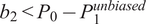 $ {b}_2<{P}_0-{P}_1^{unbiased} $
, the optimal guidance bias is
$ {b}_2<{P}_0-{P}_1^{unbiased} $
, the optimal guidance bias is
 $ {b}^{\ast }={b}_2 $
.
$ {b}^{\ast }={b}_2 $
.
If both conditions (
 $ {b}_1>{P}_0-{P}_1^{unbiased} $
and
$ {b}_1>{P}_0-{P}_1^{unbiased} $
and
 $ {b}_2<{P}_0-{P}_1^{unbiased} $
) are not met, the existence of one unique optimum implies that the maximum is given by the function’s kink, that is,
$ {b}_2<{P}_0-{P}_1^{unbiased} $
) are not met, the existence of one unique optimum implies that the maximum is given by the function’s kink, that is,
 $ {b}^{\ast }={P}_0-{P}_1^{unbiased} $
. Consequently,
$ {b}^{\ast }={P}_0-{P}_1^{unbiased} $
. Consequently,
 $ {b}^{\ast } $
equals
$ {b}^{\ast } $
equals
 $ {P}_0-{P}_1^{unbiased} $
as long as
$ {P}_0-{P}_1^{unbiased} $
as long as
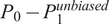 $ {P}_0-{P}_1^{unbiased} $
lies within the interval
$ {P}_0-{P}_1^{unbiased} $
lies within the interval
 $ \left[{b}_1,{b}_2\right] $
. If
$ \left[{b}_1,{b}_2\right] $
. If
 $ {P}_0-{P}_1^{unbiased} $
moves out of this interval,
$ {P}_0-{P}_1^{unbiased} $
moves out of this interval,
 $ {b}^{\ast } $
remains at the interval’s boundary.
$ {b}^{\ast } $
remains at the interval’s boundary.
Supplementary Material
To view supplementary material for this article, please visit http://doi.org/10.1017/S0022109026102580.


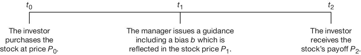


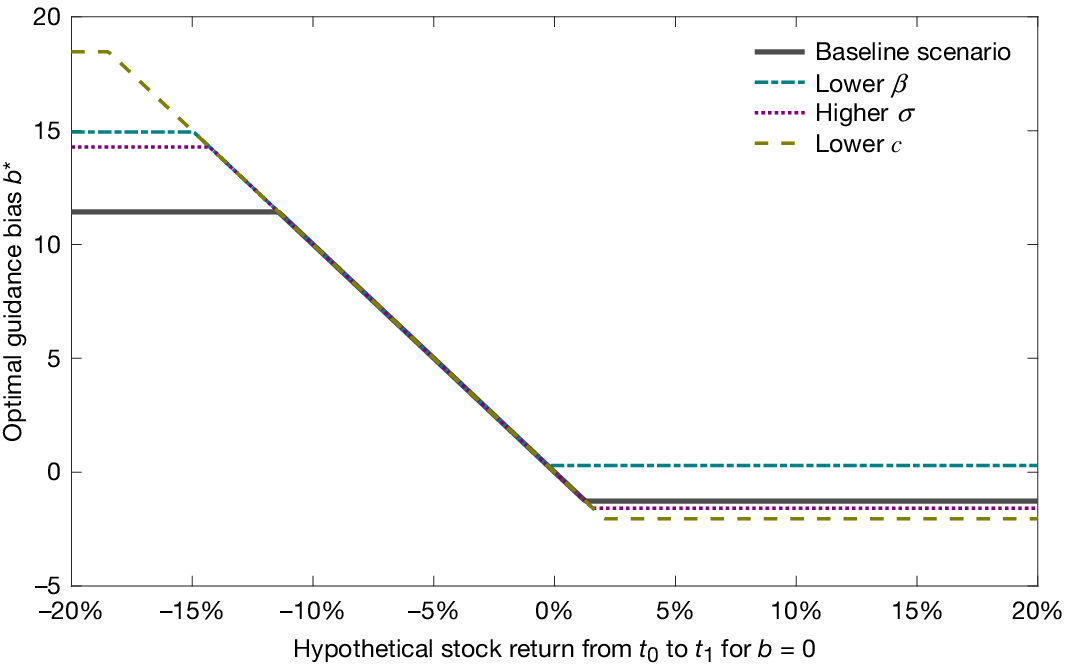


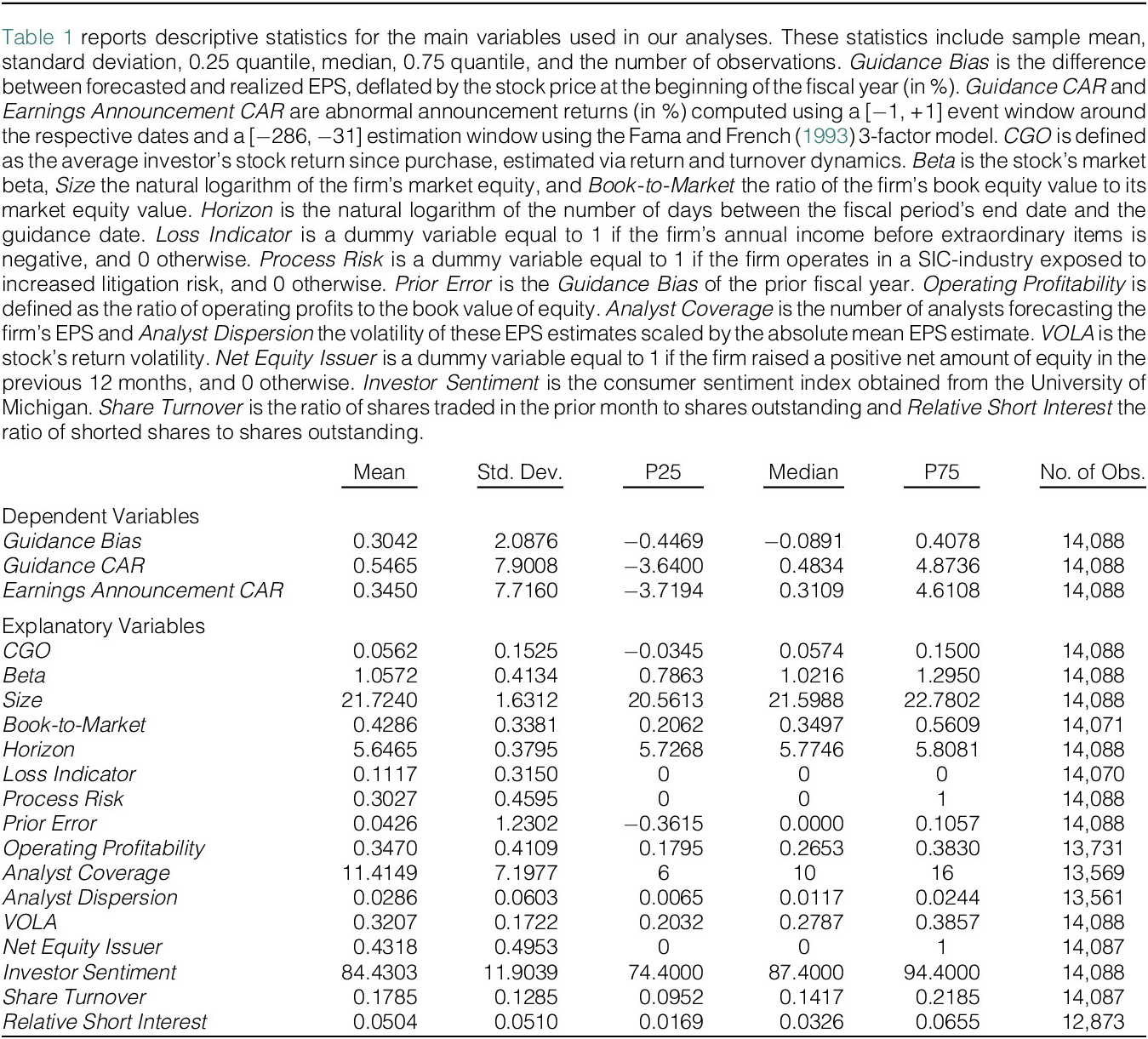
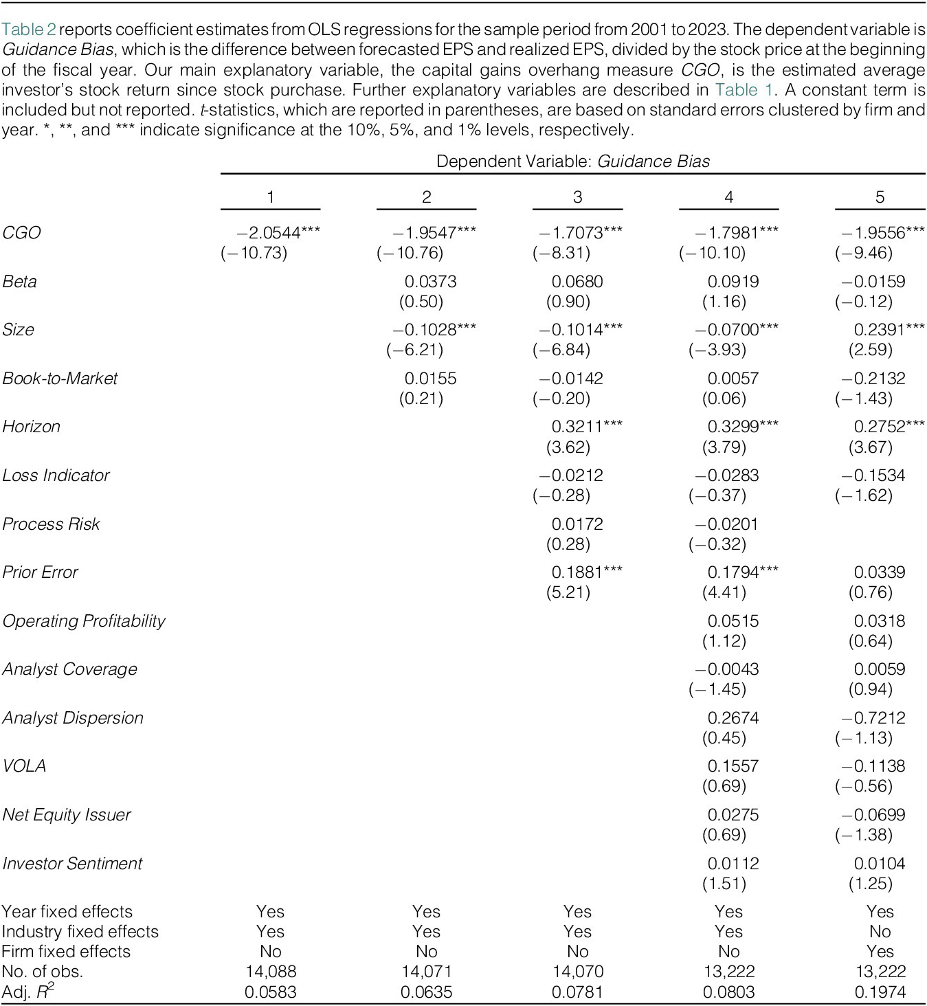
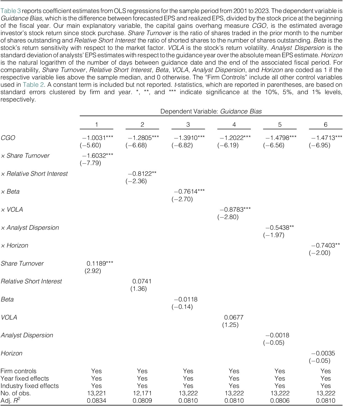
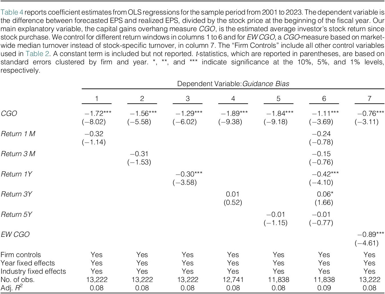
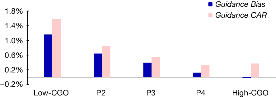


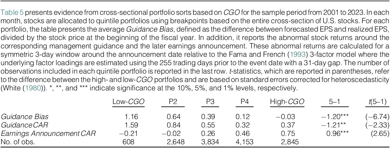
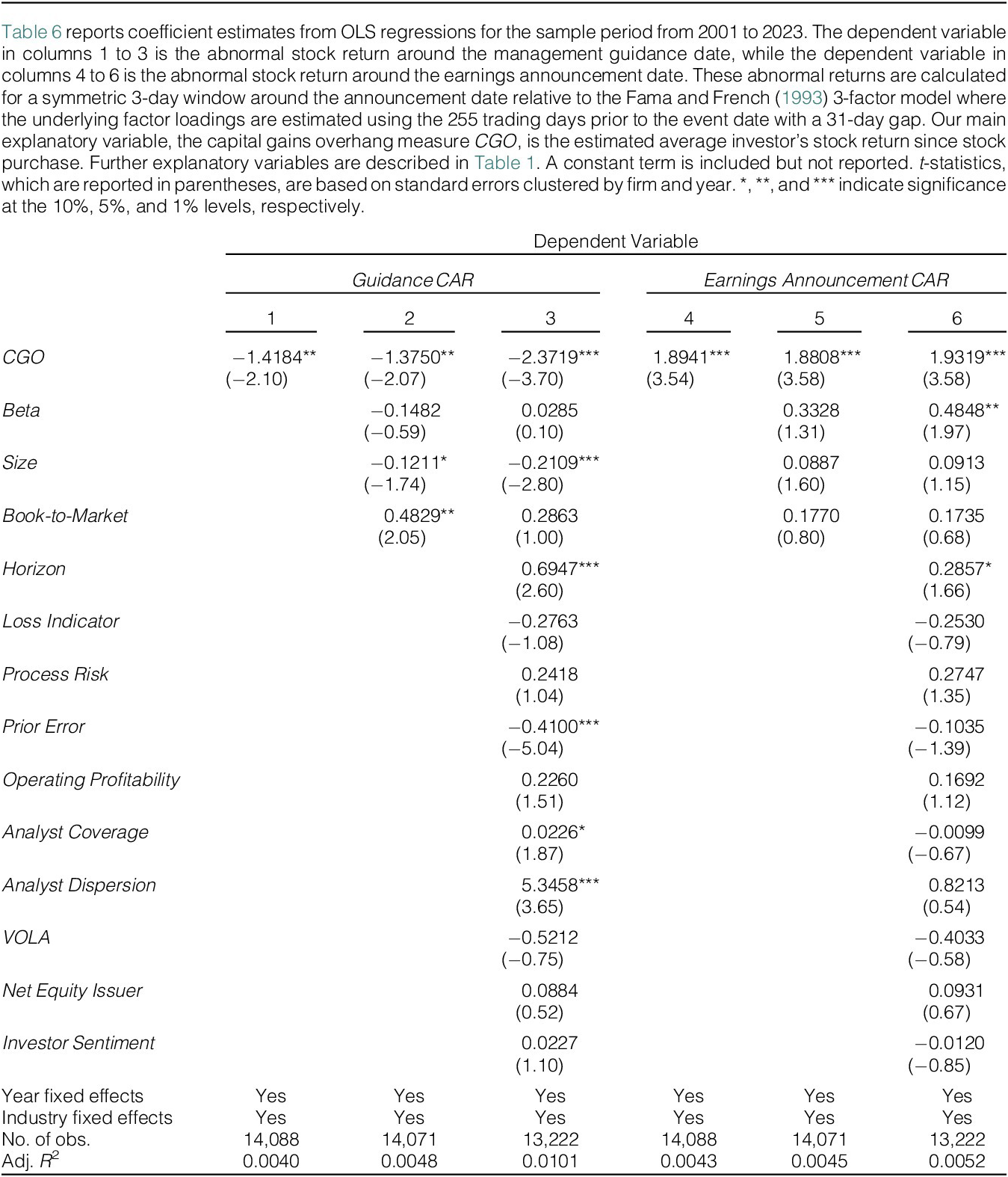
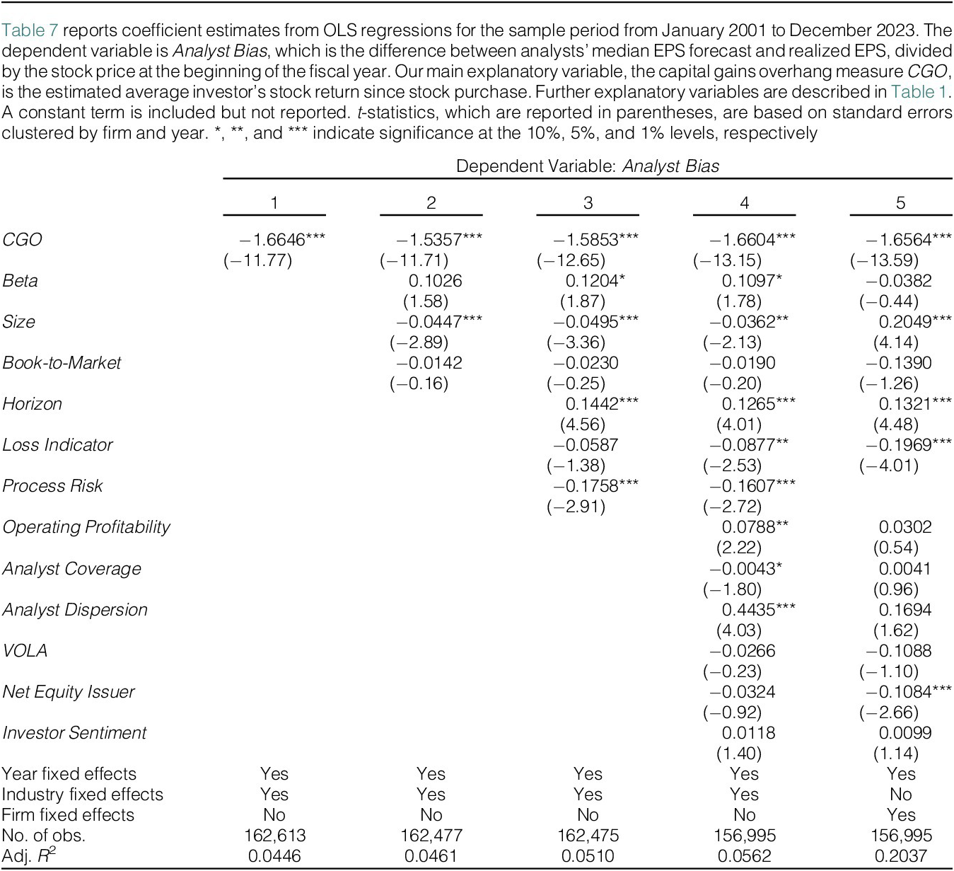


 Open access