


Introduction
The preserved Quaternary record of continental ice sheet glacial deposits in the midwestern region of North America (Fig. 1) represents a sizable amount of the unconsolidated cover spread on top of Paleozoic bedrock. The sediments comprise a series of interbedded diamicton, glaciofluvial, and related units that represent several glacial episodes during the Quaternary, containing a record of major paleoenvironmental changes during the Pleistocene (Soller et al., Reference Soller, Packard and Garrity2012). The Marine Isotope Stage (MIS) 2 record is particularly well documented, as it covers the latest advance of the Laurentide Ice Sheet (LIS) over this region (Fig. 1). Glacial deposits of MIS 6 (191–130 ka; Lisiecki and Raymo, Reference Lisiecki and Raymo2005) and older glaciations have a reduced expression at the surface north of the maximum MIS 2 glacial advance boundary (Fig. 1). Beyond this limit and toward the south, MIS 6 sediments commonly appear stacked up against a series of uplands developed on Paleozoic sedimentary rocks, for example, along the Ohio River valley in Ohio and in southern Indiana.
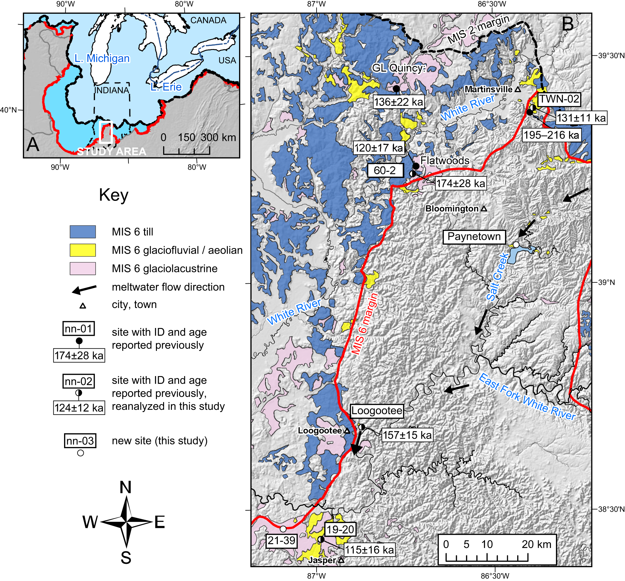
Location map. (A) The midwestern region of the United States, depicting the last two major glaciation boundaries (Marine Isotope Stage [MIS] 2 in dashed black; MIS 6 in red). Inset rectangle shows location of the study area in B. (B) Glacial deposits are shown on a hillshade digital elevation model of the region. Note meltwater flow direction across mostly unglaciated bedrock terrain. New sites where geochronology was investigated in this study are shown (open circles), along with sites where previous dating has been accomplished (closed circles), with published ages indicated near Martinsville (Loope et al., Reference Loope, Antinao, Monaghan, Autio, Curry, Grimley, Huot, Lowell, Nash and Florea2018, Reference Loope, Antinao, Jacobs, Gray and Boulding2024), glacial Lake Quincy (Wood et al., Reference Wood, Forman, Pierson and Gomez2010), Flatwoods (Jacobs et al., Reference Jacobs, Gray, Loope, Antinao and Rupp2023), and Loogootee and northwest of Jasper (Antinao et al., Reference Antinao, Davis and Loope2023). Sites with samples measured in earlier research and reanalyzed in this study are displayed by half-full circles.
MIS 6 glacial deposits in this area contain some of the most significant aquifer units near the limits of Quaternary glaciation (e.g., Yager et al., Reference Yager, Kauffman, Soller, Haj, Heisig, Buchwald, Westenbroek and Reddy2018). Characterization and understanding of these subsurface units is becoming a critical resource management issue given increased use of groundwater resources expected under future development. In addition to the regional economic significance of these deposits, improved datasets on ice-advance timing and associated ice-marginal sedimentation during MIS 6 in North America are key to develop a record of geomorphic effects of global change during this period. A well-defined record of glacial dynamics in southern Indiana can therefore complement a growing set of records in North America (e.g., Rovey and Balco, Reference Rovey, Balco and Ehlers2011), to be contrasted with global climate records (e.g., Wang et al., Reference Wang, Cheng, Edwards, An, Wu, Shen and Dorale2001; Lambert et al., Reference Lambert, Bigler, Steffensen, Hutterli and Fischer2012). Testing synchronic behavior of ice sheets in Europe and North America using these expanded datasets has the potential to address questions on correlation of the maximum extent of the LIS during MIS 6 with the maximum glacial in Eurasia (ca. 180–155 ka) or with the global penultimate glacial maximum at ca. 140 ka. Answering these questions will help in turn with calibration of models for ice-sheet evolution in North America that are needed to understand and model climate at orbital scales (e.g., Patterson et al., Reference Patterson, Gregoire, Ivanovic, Gandy, Owen, Smith, Pollard, Astfalck and Valdes2024).
During the past few decades, stratigraphic and geochronologic studies of MIS 6 and older glacial deposits in the midcontinent (e.g., Hallberg, Reference Hallberg1986; Roy et al., Reference Roy, Clark, Barendregt, Glasmann and Enkin2004; Balco and Rovey, Reference Balco and Rovey2008) have led to abandonment of the relative chronologic categories that earlier researchers defined for sediments stratigraphically below MIS 6 deposits (Chamberlin, Reference Chamberlin1895; Leverett, Reference Leverett1898; Wayne, Reference Wayne1958). Historic outcrops where older glaciation type sections were defined (e.g., Wayne, Reference Wayne1958) have been studied in detail with geochronologic techniques, including luminescence dating (e.g., Loope et al., Reference Loope, Antinao, Monaghan, Autio, Curry, Grimley, Huot, Lowell, Nash and Florea2018). One key issue has been to obtain chronologic data for sediments that are commonly assigned to the MIS 6 glaciation, which is considered one of the most expansive glacial events in the region, covering the American states of Illinois, Indiana, and Ohio (e.g., Johnson, Reference Johnson1986; Fig. 1). Only a few studies in this region have determined absolute ages in this range, mainly through optically stimulated luminescence (OSL) dating (e.g., Wood et al., Reference Wood, Forman, Pierson and Gomez2010; Webb et al., Reference Webb, Grimley, Phillips and Fouke2012; Berg et al., Reference Berg, McKay and Goble2013), in contrast to research on glacial and proglacial environments during MIS 2, which has been aided by the ability of radiocarbon dating to yield very precise dates for sediment and organic remains in proglacial environments (e.g., Heath et al., Reference Heath, Loope, Curry and Lowell2018; Loope et al., Reference Loope, Antinao, Monaghan, Autio, Curry, Grimley, Huot, Lowell, Nash and Florea2018; Dalton et al., Reference Dalton, Margold, Stokes, Tarasov, Dyke, Adams and Allard2020 and references therein). Beyond the reach of radiocarbon dating, however, fewer data are available (Dalton et al., Reference Dalton, Stokes and Batchelor2022). In particular, the single-aliquot regenerative (SAR) OSL method, whose application on small aliquots has been validated for the MIS 2 glaciofluvial and aeolian sediments in areas near the maximum MIS 2 ice margin (Loope et al., Reference Loope, Antinao, Monaghan, Autio, Curry, Grimley, Huot, Lowell, Nash and Florea2018, Reference Loope, Antinao, Jacobs, Gray and Boulding2024), has not yet been extensively tested on MIS 6 deposits. Initial data from the MIS 6 ice-marginal region in central Indiana suggest that OSL ages in quartz might display some underestimation (cf. Jacobs et al., Reference Jacobs, Gray, Loope, Antinao and Rupp2023).
The purpose of this study is to test and validate a set of luminescence dating methods for a portion of the MIS 6 LIS margin in southwestern Indiana. We assess quartz OSL and feldspar infrared-stimulated luminescence (IRSL) dating of glaciofluvial, glaciodeltaic, and aeolian sediments in a proglacial setting, both tested against a well-established soils stratigraphy (Jacobs, Reference Jacobs1994, Reference Jacobs1998; Jacobs et al., Reference Jacobs, Konen and Curry2009, Reference Jacobs, Gray, Loope, Antinao and Rupp2023) and through direct comparison at one site with cosmogenic 10Be depth-profile dating. The results indicate that luminescence signals and associated dating protocols commonly used in analysis of MIS 2 deposits in the region (e.g., Curry et al., Reference Curry, Kehew, Antinao, Esch, Huot, Caron and Thomason2021; Erber et al., Reference Erber, Kehew, Schaetzl, Gillespie, Sultan, Esch, Yelich, Curry, Huot and Abotalib2023) should be used with caution for sediments associated with older glaciations. Observed underestimation in dating with this signal (Jacobs et al., Reference Jacobs, Gray, Loope, Antinao and Rupp2023) will be addressed focusing on discriminating possible unstable signals and the saturation that more stable quartz OSL signals display. These two factors might couple to yield ages that are younger than control data. We attempt to solve this issue by studying application of feldspar post-IR IRSL dating. This new geochronologic framework will facilitate correlations with the MIS 6 record of glaciation elsewhere in the midcontinent (e.g., Webb et al., Reference Webb, Grimley, Phillips and Fouke2012; Counts et al., Reference Counts, Murari, Owen, Mahan and Greenan2015; Grimley and Oches, Reference Grimley and Oches2015) and across the Northern Hemisphere (e.g., Demuro et al., Reference Demuro, Froese, Arnold and Roberts2012).
Study area
The study area encompasses southwestern Indiana along the margins of the last two major Pleistocene glaciations (Fig. 1), where interaction occurred between ice-marginal processes and fluvial activity on bedrock-dominated topography. In much of the region, the unconsolidated sediment cover is rather thin, and bedrock appears exposed at the bottoms of valleys (Gray, Reference Gray2000). Ice advance and meltwater flow altered drainage patterns within this bedrock-dominated landscape. In some cases, the effects were temporal, blocking streams with ice or accumulating sediment in front of these dams to be removed after deglaciation (Gray, Reference Gray1988), but in other cases, drainage networks were permanently changed (Wood et al., Reference Wood, Forman, Pierson and Gomez2010; Jacobs et al., Reference Jacobs, Gray, Loope, Antinao and Rupp2023).
Prominent areas where impact of MIS 6 glaciation on the geomorphology along the ice-marginal region of southwestern Indiana has been documented are: near the city of Martinsville (Loope, Reference Loope2016; Loope et al., Reference Loope, Antinao, Monaghan, Autio, Curry, Grimley, Huot, Lowell, Nash and Florea2018, Reference Loope, Antinao, Jacobs, Gray and Boulding2024; Fig. 1); the Flatwoods area (Jacobs et al., Reference Jacobs, Gray, Loope, Antinao and Rupp2023; Loope et al., Reference Loope, Antinao, Jacobs, Gray and Boulding2024; Fig. 1); along Beanblossom Creek (Loope et al., Reference Loope, Antinao, Jacobs, Gray and Boulding2024); glacial Lake Quincy (Autio, Reference Autio1990; Wood et al., Reference Wood, Forman, Pierson and Gomez2010; Fig. 1), and near the city of Jasper in the area known as glacial Lake Patoka (Gray, Reference Gray1988; Antinao et al., Reference Antinao, Davis and Loope2023; Fig. 1). These areas display sediments ranging from diamicton to ice-proximal and valley-train glaciofluvial to proglacial glaciolacustrine and glaciodeltaic sediments, partially dissected by younger drainage or buried under a cover of MIS 2-3 loess in the west or glaciofluvial and glaciolacustrine sediments in the north.
We studied sediments from mostly valley-train and proglacial fan glaciofluvial settings (Fig. 1). Sites include one proglacial glaciolacustrine and glaciodeltaic site and one aeolian dune site along the MIS 6 ice-marginal drainage system from Martinsville to Jasper (Fig. 1; see Supplementary Data File for detailed stratigraphic columns and sedimentology data supporting our site choices). Additionally, we studied valley-train glaciofluvial deposits at the Paynetown site (Fig. 1) that carried meltwater from the ice margin as it abutted the northern edge of this region.
Glacial geomorphology and soil stratigraphic context
Mapping and identification of diamicton, glaciolacustrine, aeolian, and glaciofluvial units is based on published regional-scale mapping by Gray (Reference Gray1989), Loope (Reference Loope2016), Antinao et al. (Reference Antinao, Davis and Loope2023), and Loope et al. (Reference Loope, Antinao, Jacobs, Gray and Boulding2024) (Fig. 1). The detailed morphological setting and surficial geological unit distribution for each site is presented in the Supplementary Data File (SDF; Supplementary Fig. SDF-1). Cross sections through each site show stratigraphic relationships based on exposed sections (Fig. 2, Supplementary Fig. SDF-2) and boreholes. Cross sections (Supplementary Fig. SDF-2) also show buried soils or erosive surfaces that indicate depositional breaks or stratigraphic unconformities. The degree of soil development on stable surfaces provides a relative age for the deposits and gives guidance for cosmogenic depth-profile and luminescence dating strategies. The main pedostratigraphic features that were tracked include the Sangamon Geosol (Follmer, Reference Follmer and Porter1983; Jacobs et al., Reference Jacobs, Konen and Curry2009) and overlying MIS 2 loess layers. The Sangamon Geosol records interglacial-scale pedogenesis from MIS 5 to MIS 3 (Jacobs et al., Reference Jacobs, Konen and Curry2009). Initial luminescence chronology of some of these deposits was presented in Loope et al. (Reference Loope, Antinao, Monaghan, Autio, Curry, Grimley, Huot, Lowell, Nash and Florea2018, Reference Loope, Antinao, Jacobs, Gray and Boulding2024), Antinao et al. (Reference Antinao, Davis and Loope2023), and Jacobs et al. (Reference Jacobs, Gray, Loope, Antinao and Rupp2023) (Fig. 1). We build upon these studies by analyzing additional aliquots for samples already measured (Fig. 1, Supplementary Fig. SDF-2) or performing different measurement protocols. Coupled methods are applied to the studied sections to build a robust chronologic framework; in our case, quartz OSL and feldspar IRSL are both used to determine burial chronology, and cosmogenic 10Be depth-profile dating is tested at one site as an independent geochronometer.
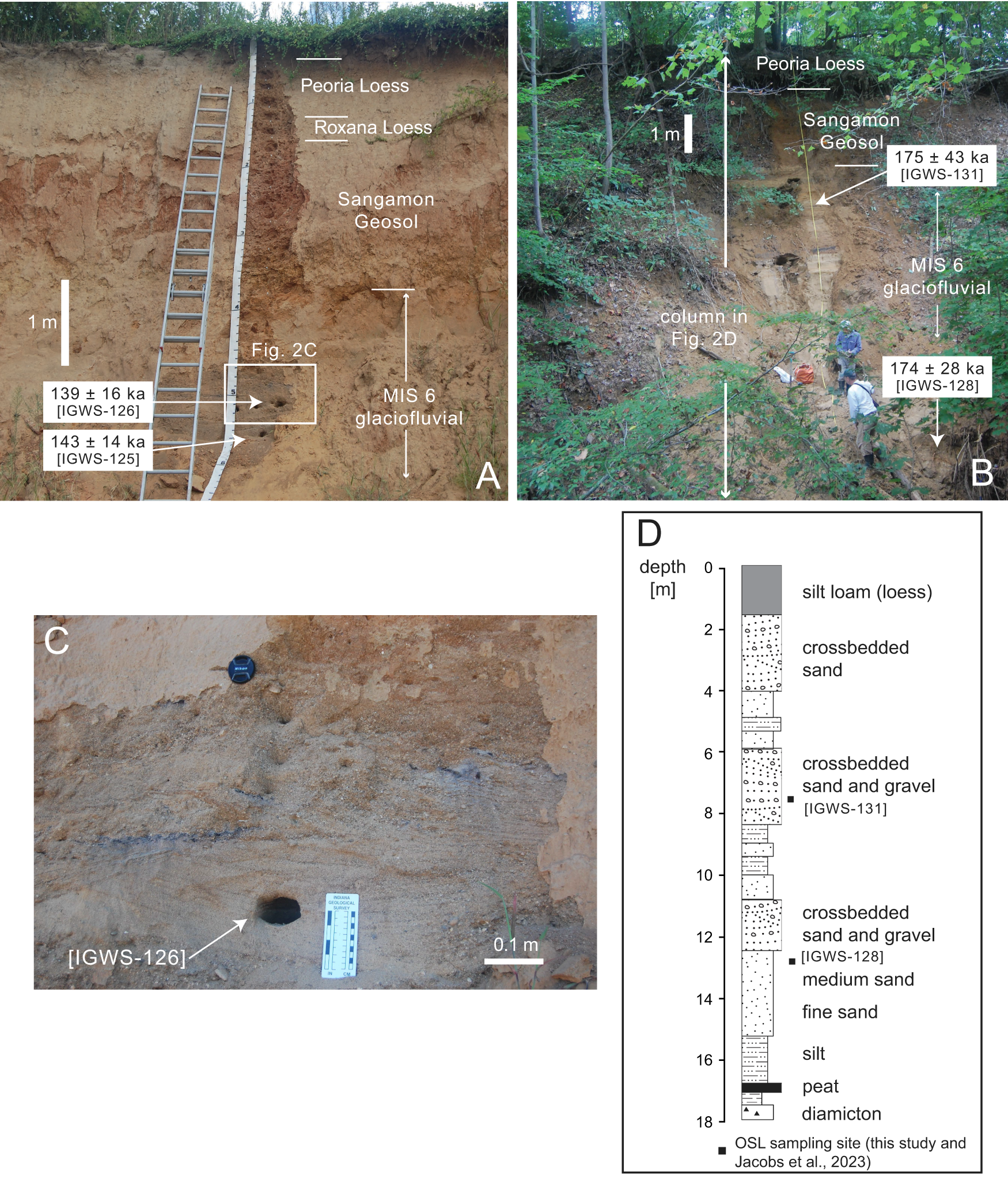
Select field site photographs and lithologic data. Site location in Figure. 1; additional photographs in Supplementary Figure. SDF-3. (A) Loogootee site. Note scale on the photograph, thickness of Sangamon Geosol, and location of samples previously dated (ages shown for data in Antinao et al. [Reference Antinao, Davis and Loope2023]) and re-analyzed in this study. (B) The 60-2 site in Flatwoods. Note thickness of Sangamon Geosol and location of samples previously dated (ages shown for data in Jacobs et al. [Reference Jacobs, Gray, Loope, Antinao and Rupp2023]) and re-analyzed in this study. (C) Detail for location of sample IGWS-126, highlighting placement below the lower boundary of the Bt soil horizon. (D) Lithologic column for section 60-2 (B), displaying location of studied luminescence samples. MIS, Marine Isotope Stage; OSL, optically stimulated luminescence.
Study sites
Site 1 (TWN-02 borehole; Fig. 1, Supplementary Fig. SDF-1) is a shallow borehole drilled into a glaciodeltaic and glaciolacustrine sequence of sand and silt that was sampled for cosmogenic depth-profile dating and for luminescence dating at depths ∼6 m below the surface (Supplementary Fig. SDF-2). An age of 131 ± 11 ka by OSL on quartz (Loope et al., Reference Loope, Antinao, Monaghan, Autio, Curry, Grimley, Huot, Lowell, Nash and Florea2018; Fig. 1) was determined for one sample from this borehole, which was measured again in the present study for quartz OSL and feldspar IRSL dating. The depositional environment of the whole terrace (Supplementary Fig. SDF-2) is interpreted as a proglacial outwash fan at the base, grading upward to a sand-rich glaciodeltaic and glaciolacustrine terrace. Glaciolacustrine deposition developed on a local drainage obstructed by earlier outwash deposition and proximity of the ice sheet. The terrace was abandoned once the MIS 6 ice margin retreated north from the local maximum, located about 5 km to the north and west; the ice did not override the site. A complete Sangamon Geosol has developed and is preserved at this site on a stable geomorphic surface, away from gullies.
Site 2 (60-2 section; Figs. 1 and 2B and D, Supplementary Figs. SDF-1–SDF-3) is a natural section that was described and sampled for luminescence dating at depths of 7.5 and 12.5 m below the surface (Fig. 2D, Supplementary Fig. SDF-2). The section consists of ∼15 m of cross-bedded sand and gravel deposited directly on top of an organic layer atop a diamicton (Jacobs et al., Reference Jacobs, Gray, Loope, Antinao and Rupp2023; Fig. 2B and D, Supplementary Fig. SDF-2). The exposed section sits at the incised top surface of a proglacial, outwash fan surface emanating from the ice margin ∼1 km to the north, with a low slope toward the south, where the proglacial drainage ended at a sinkhole (Supplementary Fig. SDF-2). A complete Sangamon Geosol is preserved at this site.
Site 3 (Loogootee section; Figs. 1 and 2A and C, Supplementary Figs. SDF-1–SDF-3) is located in a gravel pit on a flat glaciofluvial terrace sourced from an outwash channel originating from the MIS 6 ice margin 8 km to the north, where an exposure of ∼7 m reveals a section with predominantly cross-bedded sand and gravel with a complete Sangamon Geosol developed in the glaciofluvial terrace (Fig. 2A and C). As in the previous two sites, thin MIS 3 (Roxana Loess) and 2 (Peoria Loess) layers appear on top of the Sangamon Geosol.
Site 4 (Paynetown borehole; Fig. 1, Supplementary Figs. SDF-1 and SDF-2) is located on a flat glaciofluvial terrace covered with a colluvial wedge, perched on the north side of a bedrock valley. The terrace represents aggradation of a valley-train outwash channel coming from the MIS 6 ice margin sourced about 50 km to the north (Loope et al., Reference Loope, Antinao, Jacobs, Gray and Boulding2024).
Site 5 (borehole 19-20; Fig. 1, Supplementary Figs. SDF-1 and SDF-2) is located on a glaciofluvial plain, covered with transverse aeolian dunes (Antinao et al., Reference Antinao, Davis and Loope2023). The site is at the eastern edge of the glaciolacustrine plain known as glacial Lake Patoka, at ∼150 m above sea level (m asl) and bounded on the north by a morainic ridge (Antinao et al., Reference Antinao, Davis and Loope2023). A complete Sangamon Geosol developed on the dunes is also preserved on this site, covered with MIS 2 loess (Antinao et al., Reference Antinao, Davis and Loope2023; Supplementary Fig. SDF-2E). The relief in the subdued dune landscape is about 6 m (Supplementary Fig. SDF-2).
Site 6 (borehole 21-39; Fig. 1, Supplementary Figs. SDF-1 and SDF-2) is located on a relatively flat surface on the bed of a glacial lake (Gray, Reference Gray1988; Antinao et al., Reference Antinao, Davis and Loope2023) reaching bedrock at a depth of 53.3 m, penetrating a package of mostly silt and sand. The depositional environment is interpreted as a proglacial glaciodeltaic package composed of sand that grades upward into glaciolacustrine silt and sand. Sedimentation was caused by the obstruction of local drainage both by glaciodeltaic sedimentation and the MIS 6 ice at maximum extent (Gray, Reference Gray1988). Sediment composition is dominated by glacially transported sand from the north, with a smaller proportion of locally derived lithologies. The local maximum ice margin is located about 3 km to the north and west, and the ice did not override the site (Supplementary Fig. SDF-2). A complete Sangamon Geosol is preserved on this site (Supplementary Fig. SDF-2).
Methods
Luminescence dating
A total of 13 samples were selected for this study (Figs. 1 and 2, Supplementary Fig. SDF-1). Sampling was carried out by inserting metal tubes perpendicularly into cleaned exposed sections or by inserting tubes longitudinally into extruded cores or by direct collection from shielded shallow coring probe liners. Sample preparation was carried out under dim filtered sodium-vapor light conditions at the Indiana Geological and Water Survey (IGWS) Luminescence Laboratory. Luminescence measurements were made using Lexsyg Smart TL/OSL readers. Details on preparation protocols, luminescence stimulation sources, and emission filters can be found in the Supplementary Data File (Supplementary Table SDF-1). Equivalent (burial) doses were obtained using the SAR protocol (Murray and Wintle, Reference Murray and Wintle2000, Reference Murray and Wintle2003) for blue-light OSL (hereafter referred to as OSL) in quartz samples and using a modified post-IR IRSL SAR protocol from Buylaert et al. (Reference Buylaert, Murray, Thomsen and Jain2009, Reference Buylaert, Jain, Murray, Thomsen, Thiel and Sohbati2012) on feldspar samples, with an initial IR stimulation at 50°C followed by IR stimulation at 200°C (post-IR IRSL200). OSL or IRSL measurements were completed on small aliquots (i.e., 10–40 mineral grains spread around a 2-mm-diameter zone at the center of stainless-steel disks; Supplementary Fig. SDF-4) of 180–220 micron sand due to the expected incomplete bleaching in the proximal glaciofluvial and glaciodeltaic environment (e.g., Curry et al., Reference Curry, Kehew, Antinao, Esch, Huot, Caron and Thomason2021; Erber et al., Reference Erber, Kehew, Schaetzl, Gillespie, Sultan, Esch, Yelich, Curry, Huot and Abotalib2023; Jacobs et al., Reference Jacobs, Gray, Loope, Antinao and Rupp2023).
In the case of quartz OSL analysis, aliquots were initially screened for the shape of the OSL decay curve measured as natural (Ln) and after a test dose (Tn) of ∼12 Gy (Table 1A). If both the Ln and Tn signals were above background and considered not affected by presence of slow or medium decay components (cf. Jain et al. Reference Jain, Murray and Bøtter-Jensen2003) upon visual examination of the OSL decay curves, then all the regenerative steps in the SAR procedure were continued for that aliquot (Table 1B). In case the signal was dim or the shinedown curve showed indication of slow or medium components, the SAR portion was not run at all, ensuring optimization of reader time allocation (a flowchart of this protocol is described in Supplementary Fig. SDF-41). For quartz OSL analysis, dose-recovery tests were performed in one sample per site and a preheat plateau experiment was performed at the aeolian sample site to validate our approach and to establish optimal preheat conditions (Wintle and Murray, 2006). Selected samples were tested using linear-modulated OSL to observe distinct signal components and assess their dominance (e.g., Jain et al., Reference Jain, Murray and Bøtter-Jensen2003). For the post-IR IRSL200 SAR protocol in feldspar (Table 2), fading measurements were carried out for every aliquot. Fading rates (g-values) were calculated using a dose of 27 Gy (test dose of 13 Gy), following the method of Auclair et al. (Reference Auclair, Lamothe and Huot2003). Measurements were made approximately 102, 104, and 105 s after irradiation with the beta source, storing the sample outside the readers to optimize instrument usage time. Precise lengths for fading periods therefore varied slightly from sample to sample (see Supplementary Fig. SDF-5).
Protocol used for single-aliquot regenerative (SAR) procedure in quartz.
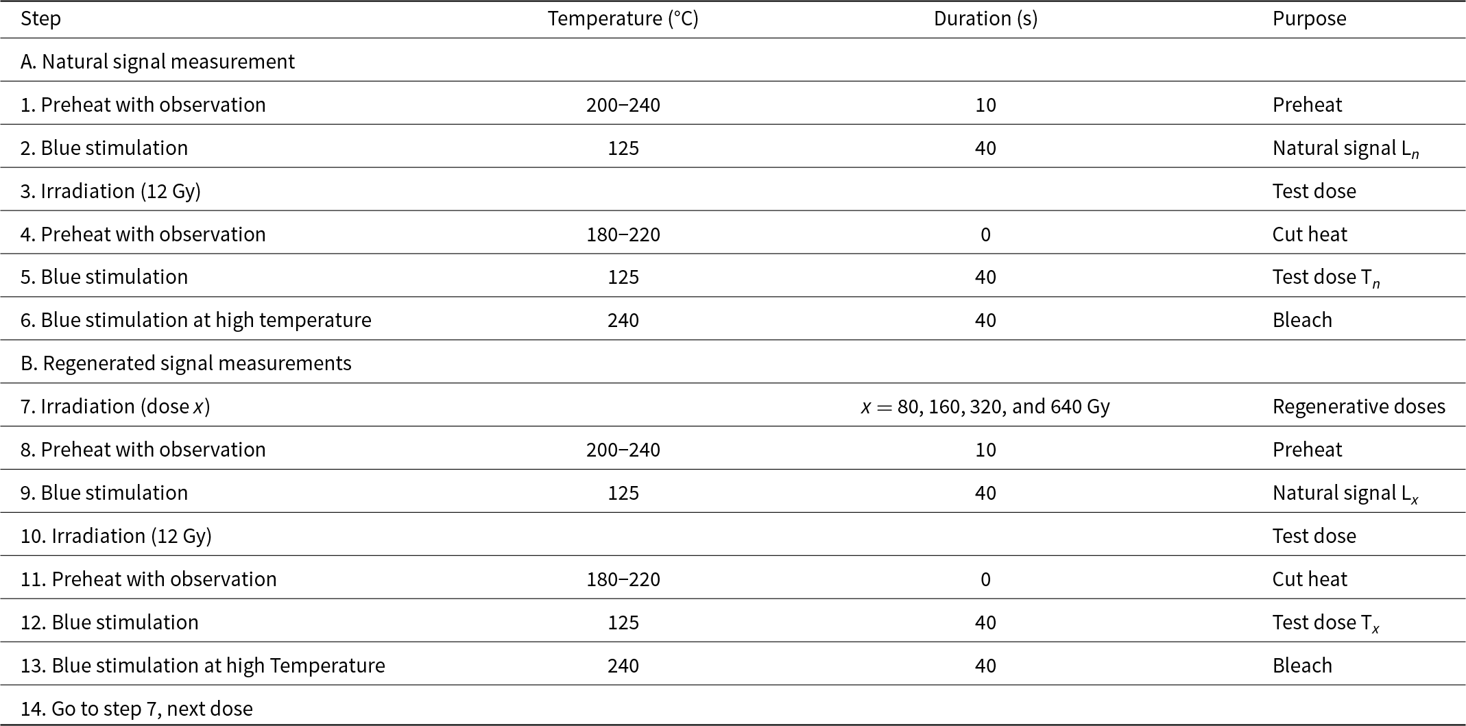
aRegenerative steps (7–13) were administered for each aliquot at four cycles at 80, 160, 320, and 640 Gy, only if initial observations Ln, Tn showed no indication of the signal being affected by slow or medium components.
Protocol used for single-aliquot regenerative (SAR) post-IR infrared-stimulated luminescence (IRSL200) procedure in feldspar.a
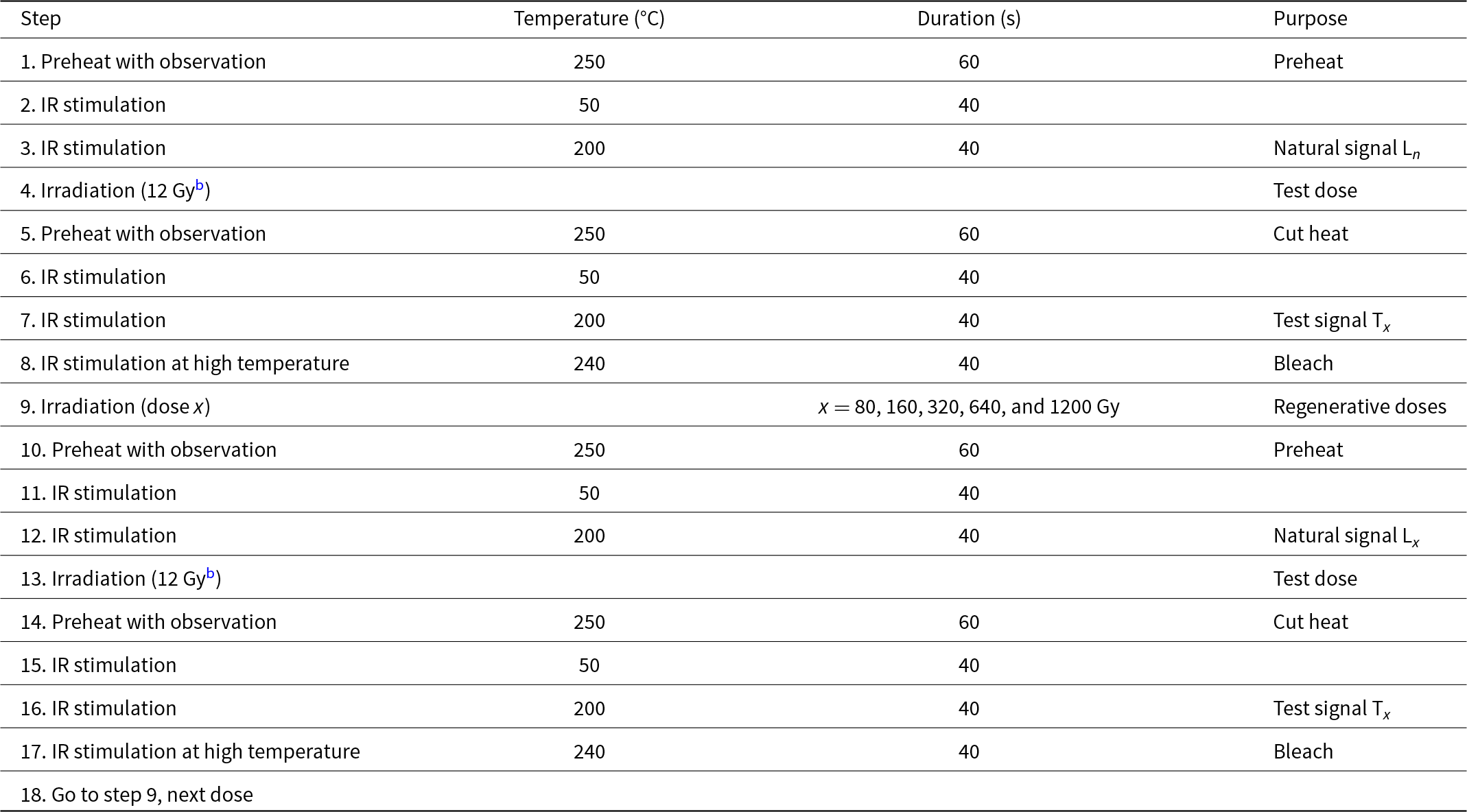
a Regenerative steps were administered for each aliquot at four cycles at 80, 160, 320, and 640 Gy (On a few samples, additional 1200 Gy were recovered.) Test dose in a few experiments was 6 Gy, and for a fading comparison experiment, it was changed to 63 Gy.
b A few runs with test dose 6 and 27 Gy.
After luminescence measurements concluded and data files were generated by the reader, output files were loaded as *.binx files in Analyst software (Duller, Reference Duller2015), and acceptance criteria were applied to each aliquot. Aliquots were accepted for further analysis if the recuperation signal was less than 5% of the natural signal, the maximum test dose error was lower than 10%, the natural test signal was more than 3-sigma above the background, and recycling ratio values were within 10% of unity. In the analysis of equivalent dose distributions for the feldspar post-IR IRSL200 protocol, we selected the subset of non-fading aliquots (those with g-values within 1-sigma of zero). Dose distributions were modeled using both the minimum age model (MAM; Galbraith et al., Reference Galbraith, Roberts, Laslett, Yoshida and Olley1999) and the central age model (CAM; Galbraith et al., Reference Galbraith, Roberts, Laslett, Yoshida and Olley1999) in the R Luminescence package (Kreutzer et al., Reference Kreutzer, Schmidt, Fuchs, Dietze, Fischer and Fuchs2012). The choice of model was determined by the skewness of the dose distribution, and the observed overdispersion when a CAM model was applied. These factors were usually consistent between samples from a similar depositional environment; that is, glaciofluvial sediments usually showed positively skewed distributions to be analyzed using MAM, and glaciodeltaic and aeolian samples showed normal distributions that were analyzed with CAM. Exceptions are discussed.
Samples were taken from the sediment surrounding the OSL/IRSL dating samples to estimate the environmental dose rate during burial. The concentration of elements with naturally emitting radiation was measured through inductively coupled plasma (ICP)-atomic emission spectrometry (AES) (K) and ICP-mass spectrometry (MS) (U, Th) and is presented in Table 3. Internal dose rate was considered negligible in quartz. Internal K content in feldspar is estimated at 10 ± 2% (Smedley et al., Reference Smedley, Duller, Pearce and Roberts2012), which yields an internal dose rate of 0.676 ± 0.136 Gy/ka (not shown on Table 3 but incorporated into final estimate of environmental dose rate in Table 4). Water content was estimated based on both the measured water weight content from the site (Table 3; determined through weight loss upon oven drying samples at 40°C temperature for 7 days) and assumptions about the geologic history of the site. A value of 9 ± 2% was used for samples in in the vadose zone (roughly shallower than 7–8 m), while a value of 22 ± 4% was used for samples at depths below the water table depth. An intermediate value of 18 ± 4% was used for samples between 8 and 20 m. Cosmic ray dose rates were estimated using latitude, longitude, elevation, and depth of sampling sites using the parameters of Prescott and Hutton (Reference Prescott and Hutton1994). External dose rates were calculated using all the above data (Table 3) with the online code DRAC (Durcan et al., Reference Durcan, King and Duller2015). The same code calculated age estimates using the equivalent dose data.
Field (location, depth in section, elevation) and analytical (inductively coupled plasma– mass spectrometry [ICP-MS] U, Th, Rb, and inductively coupled plasma–atomic emission spectrometry [ICP-AES] %K) data used to determine external dose rate for quartz optically stimulated luminescence (OSL) and feldspar infrared-stimulated luminescence (IRSL) dating.a
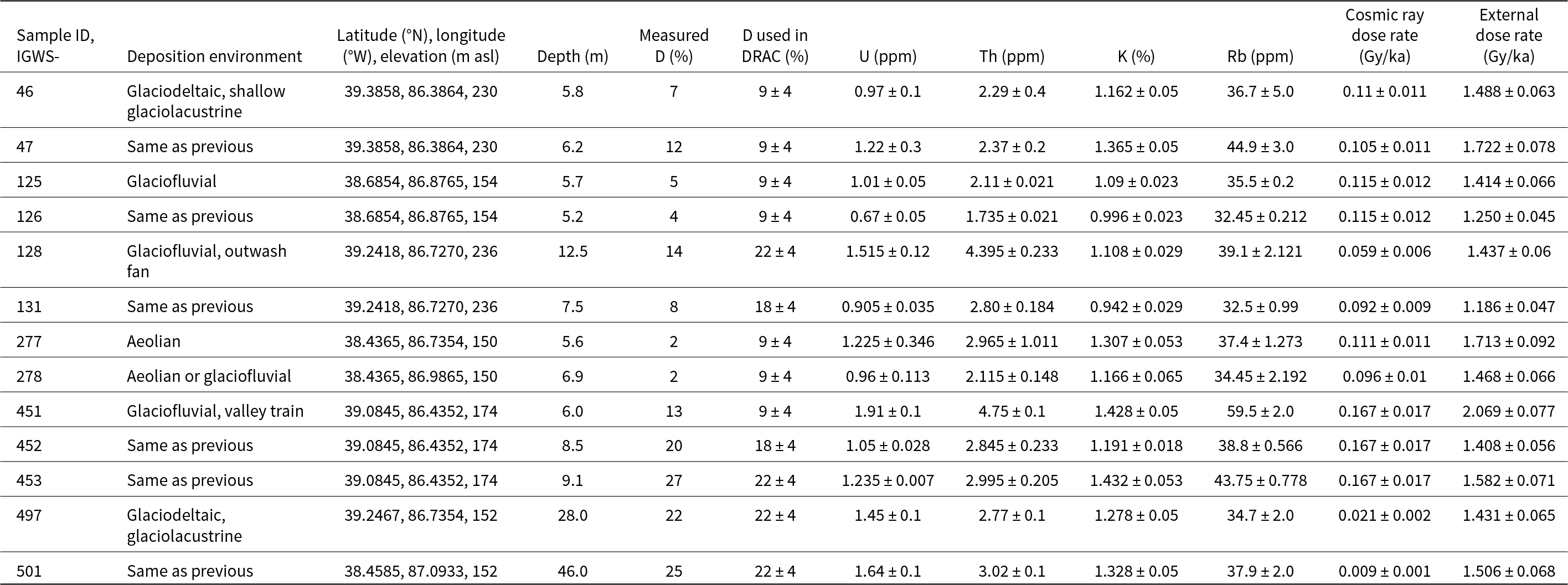
a Uncertainty in analytical values obtained by replicating (n ≥ 2) subsamples and determining mean and standard deviation of these data. D, water content (%) = 100 * weight water/weight dry sediment. Calculations made with DRAC, online code (Durcan et al., Reference Durcan, King and Duller2015).
Chronological data: feldspar infrared-stimulated luminescence (IRSL) dating (post-IR IRSL200; in the case of sample IGWS-47, IRSL at 50°C), and quartz optically stimulated luminescence (OSL) ages.
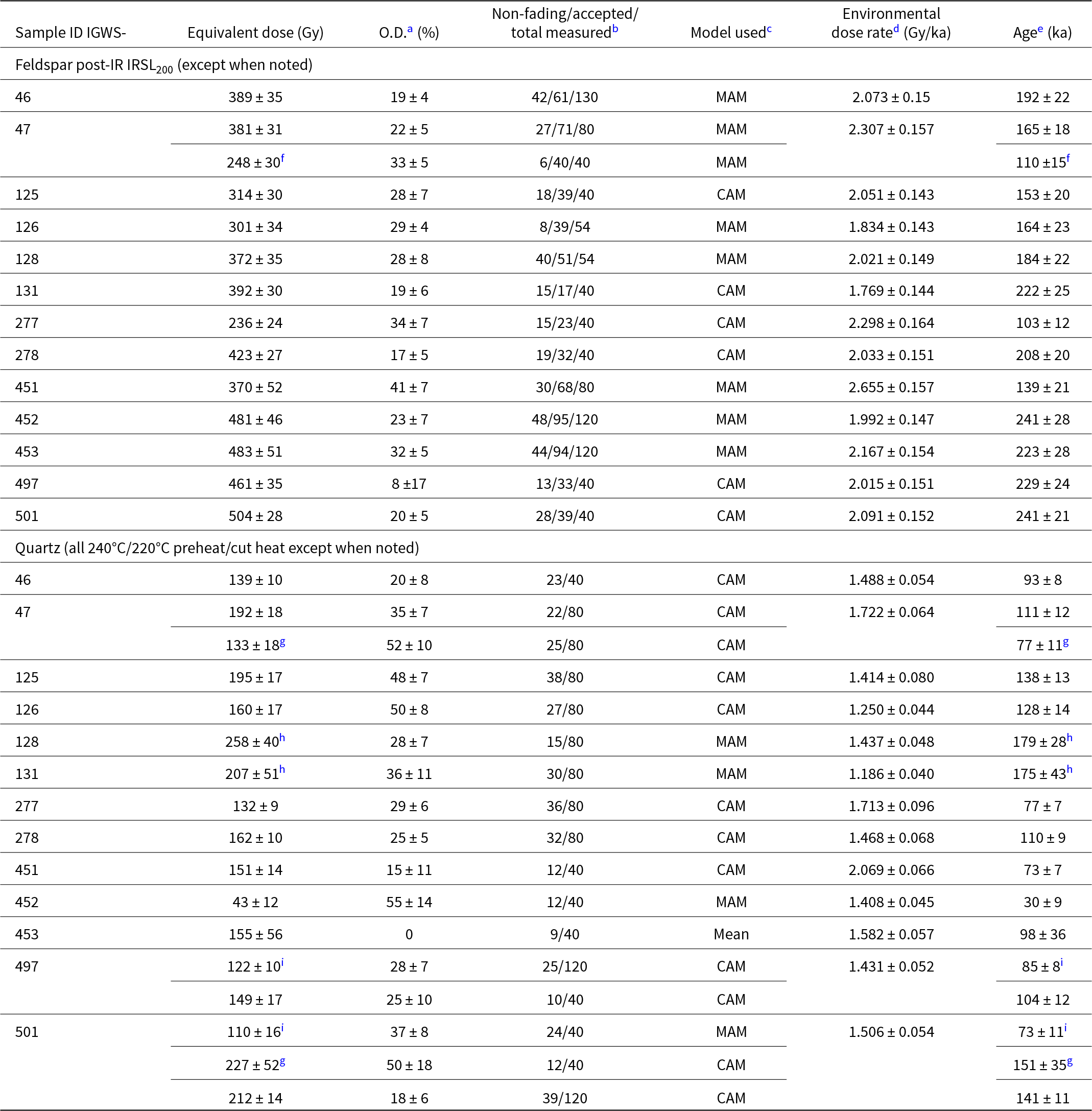
a For feldspar data, overdispersion obtained from the non-fading aliquot dose distribution using a central age model (Galbraith et al., Reference Galbraith, Roberts, Laslett, Yoshida and Olley1999).
b For all samples, the accepted aliquots number includes those with saturated natural signal.
c CAM, central age model; MAM, minimum age model. Both from Galbraith et al. (Reference Galbraith, Roberts, Laslett, Yoshida and Olley1999).
d Environmental dose rate obtained from Table 3, adding internal dose rate in the case of feldspar data.
e Reference date for ages: all samples collected between 2019 and 2021.
f IRSL 50°C, not corrected for fading.
g Higher preheat (240°C/220°C) with 3 s short-shine at low power (2 mW/cm2).
h Lower preheat settings (220°C/200°C; data from Jacobs et al. [Reference Jacobs, Gray, Loope, Antinao and Rupp2023], recalculated dose rate).
i Lower preheat settings (200°C/180°C).
Cosmogenic depth-profile dating
A direct comparison of luminescence dating with cosmogenic 10Be depth-profile dating was completed at site 1 (Fig. 1; shallow borehole TWN-02). A cosmogenic 10Be depth-profile model estimates cosmogenic nuclide inheritance as well as exposure age and erosion rate of the landform surface (e.g., Hidy et al., Reference Hidy, Gosse, Pederson, Mattern and Finkel2010). The procedure aimed to quantify duration of surface exposure and Sangamon Geosol development in glaciofluvial/glaciodeltaic sand before deposition of the loess layers that buried the geosol. The presence of complete soil horizonation at this site indicates minimal erosion; a maximum erosion of 10 cm was included in model parameters. The exposure age of the Sangamon Geosol was calculated considering isotope production below 1.5 m of Peoria Loess deposited between 29 and 21 ka (25 ± 4 ka) (Loope et al., Reference Loope, Antinao, Monaghan, Autio, Curry, Grimley, Huot, Lowell, Nash and Florea2018). The 10Be isotopes were analyzed in quartz sand (150–710 micron) samples from multiple depths within the geosol. Purification of quartz was accomplished at IGWS, and preparation of targets for cosmogenic analysis was performed at the Desert Research Institute (Reno, NV), where 10Be was isolated from pure quartz using chromatographic columns and chemical extraction. Beryllium oxide targets were loaded and analyzed at Lawrence Livermore National Laboratory. Detailed analytical protocols are available in the Supplementary Data File. Once 10Be concentration values were obtained, the 10Be production since 25 ± 4 ka was subtracted for all sample depths to account for burial of the Sangamon Geosol by 1.5 m of MIS 2 Peoria Loess. The corrected data were used as input in the model (see Table 5 and Supplementary Table SDF-2 for full dataset). We use the constrained Monte Carlo approach of Hidy et al. (Reference Hidy, Gosse, Pederson, Mattern and Finkel2010) to analyze the 10Be depth-profile results, coded in Matlab. The code models surface ages allowing explicit input of geologic variables, such as surface erosion rate and subsurface density and their probability distributions, reflecting uncertainties from field and laboratory analyses (Hidy et al., Reference Hidy, Gosse, Pederson, Mattern and Finkel2010).
Cosmogenic 10Be depth profile data for TWN-02 core, displaying the measured concentration (detailed data in Table SDF-2), the adjusted concentration removing 10Be accumulation under loess cover since 25 ± 4 ka, and relative uncertainty in concentration, the latter two used in model.a
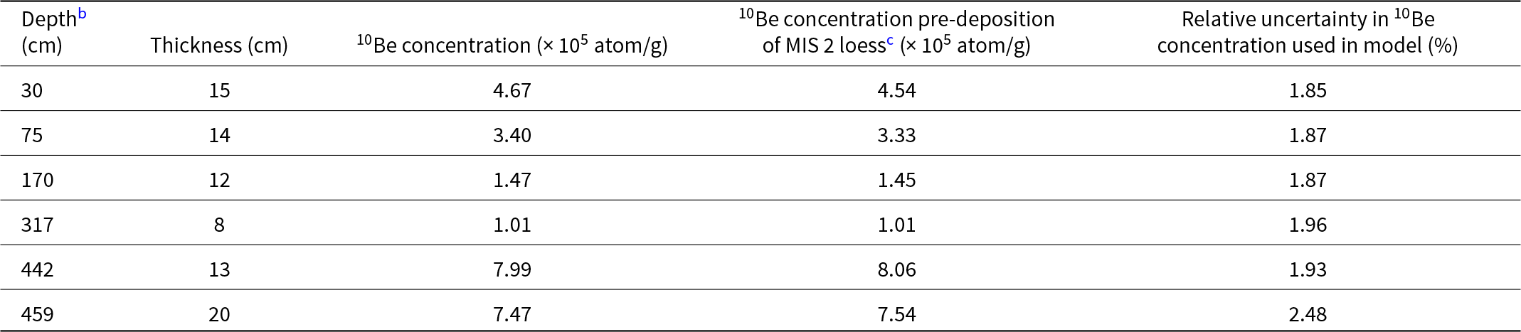
a Location of core is at 39.3858°N, 86.3864°W, at 230 m asl, with topography shielding factor estimated at 0.99.
b Depth is measured from top of the Sangamon Geosol (approximately 1.5 m below modern surface), used in modeling. Reported top level and thickness of sampled interval.
c Used in the modeling input parameters. MIS, Marine Isotope Stage.
Results
We introduce the luminescence characteristics data using a subset of pilot samples first, followed by our full luminescence dataset, and then the cosmogenic geochronologic data for site 1 (TWN-02; Fig. 1). Finally, the whole geochronologic dataset is presented in stratigraphic context for each site.
Luminescence dating
Quartz OSL signal properties
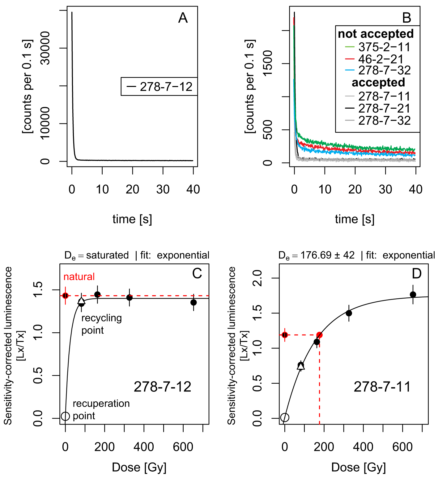
OSL decay and dose–response curves. OSL measurements were assessed from between 40 and 120 aliquots for most samples (Table 4), initially testing different preheat parameters (Table 1). For all preheat settings, the analyzed aliquots displayed relatively dim signal, and many aliquots showed only ∼500 or fewer counts in the first 0.1 s of stimulation. Three types of aliquots were identified: aliquots with bright signal, with clear dominance of the fast component (Fig. 3A); aliquots displaying weak signal, with dominance of a fast component, which were accepted for the full SAR measurement set (Fig. 3B); and aliquots displaying medium and slow components (e.g., color set on Fig. 3B) that were not accepted. Recuperation values ranged from 0% to 3% in most accepted aliquots, being closer to 0% in most cases. The onset of saturation is highly variable; for some aliquots, saturation is reached at about 100 Gy (e.g., aliquot 12 in Fig. 3C), while for others, saturation is well beyond 250 Gy (Fig. 3D). Some samples display aliquot values of 2D 0 beyond 250 Gy, therefore allowing interpolation of Ln values in the range 0–250 Gy, although most aliquots display 2D 0 below this value (see Supplementary Fig. SDF-38, for sample IGWS-501).
Quartz optically stimulated luminescence (OSL) decay and dose–response curves for sample IGWS-278. All runs with preheat/cut heat settings of 240°C/220°C. (A) OSL decay curve for sample IGWS-278, run 7, aliquot 12, 13 Gy dose. (B) OSL decay curve for samples IGWS-278, run 7, aliquots 11, 21, 32; IGWS-46, run 2, aliquot 21, IGWS-375, run 2, aliquot 11. (C) Dose–response curve for same aliquot as in A. (D) Dose–response curve for aliquot 278-7-11 (in B).
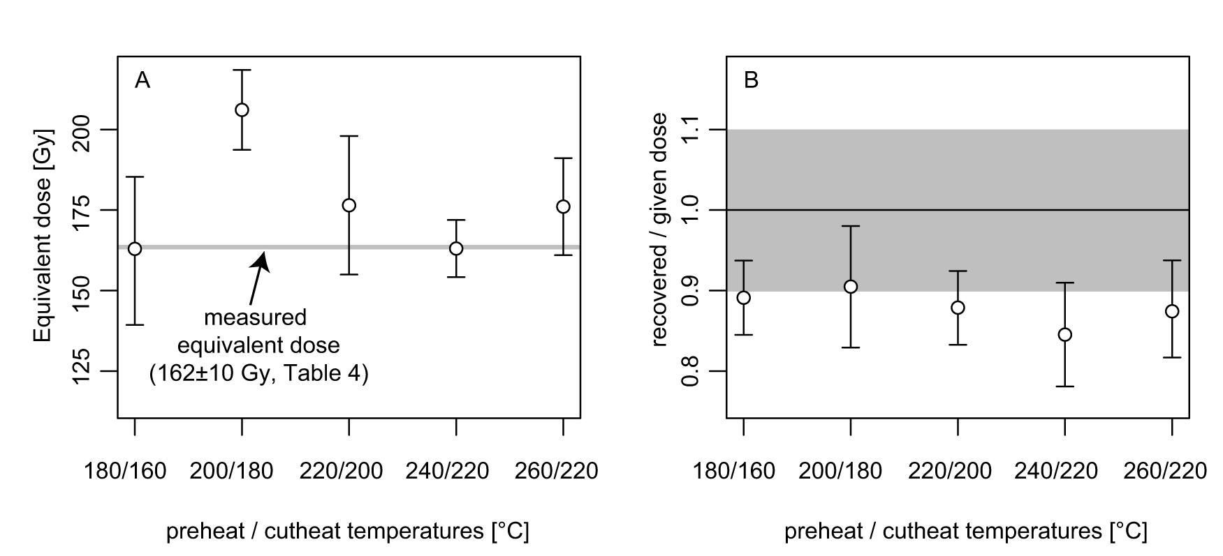
Preheat plateau and dose-recovery tests. Tests were conducted on sample IGWS-278 (Fig. 4), taken from what is considered well-bleached sediment at the base of a dune (site 6, borehole 19-20) on top of waning glaciolacustrine or glaciofluvial deposition (Antinao et al., Reference Antinao, Davis and Loope2023; Supplementary Fig. SDF-2). Preheat plateau tests with preheat temperatures between 180°C and 260°C were carried out (Fig. 4), with cut heat values 20°C below preheat, except for the last set (Fig. 4A). The higher preheat settings (240°C, 260°C preheat) yield values that are closer to the estimated dose based on soils and landform position. A higher spread and lack of consistent behavior were observed on the lower temperature end of the dataset. Dose-recovery tests were also performed (Fig. 4B) at different preheat settings after irradiation with 127 Gy. All dose-recovery tests underestimated the given dose, although all of them are within 10% of it considering uncertainty at ±1-sigma. Saturated recovered signal after irradiation at 127 Gy is observed in these experiments; this is expected given the wide set of D 0 values obtained for dose–response curves in the quartz OSL in the region (see Supplementary Fig. SDF-38, for sample IGWS-501).
Preheat plateau (A) and dose-recovery (B; 127 Gy) test for sample IGWS-278. Only accepted aliquots with fast-component predominance were accepted in the analysis (between 11 and 13 aliquots out of 40 for all temperatures).
Aliquot selection criteria assessment and linear-modulated–OSL experiments. A fast ratio (FR) analysis (Durcan and Duller, Reference Durcan and Duller2011) was performed for one run (40 aliquots) of sample IGWS-278, to support our choice of selection criteria to complete the SAR protocol after the natural signal was evaluated, as stated in the Methods section (Table 1). Preheat/cut heat settings at 240°C/220°C were used, followed by linear-modulated (LM) OSL tests on the same aliquots (Fig. 5). Aliquot selection using the FR criterion of Durcan and Duller (Reference Durcan and Duller2011) resulted in a rather small dataset (n = 6, data points above the dashed line in Fig. 5A) compared with the number selected using our criteria outlined in the “Methods” (n = 17, closed symbols on Fig. 5A). Given that the initial screening in all samples detected the presence of medium or slow components (Fig. 3B), we carried out experiments with LM-OSL analysis to discriminate the presence of these different signals in the studied aliquots (Fig. 5B–E). LM-OSL signal was assessed at two different preheat values: one set measured at 125°C after preheat at 240°C, the other after a preheat of 180°C. All LM-OSL tests were performed after irradiation with 217 Gy, linearly increasing power on the blue LEDs from 0 to 100 mW/cm2, between 0 and 100 s (Fig. 5B–E).
Fast ratio (FR) and linear-modulated optically stimulated luminescence (LM-OSL) data for sample IGWS-278. (A) FR for IGWS-278 for 40 individual aliquots on run 6 (240°C/220°C preheat settings). The FR was calculated for the natural OSL decay curve (open symbols) and a 127 Gy dose (filled symbols) given only to the aliquots selected using the manual discrimination described in the “Methods.” The threshold FR = 20 suggested by Durcan and Duller (Reference Durcan and Duller2011) is indicated with a dashed line. Note aliquots highlighted in B (no. 19), C (no. 28), D (no. 29), and E (no. 31). (B) LM-OSL plot for aliquot 19. Inset showing a detail of the first 20 s of illumination ramp, highlighting two distinct peaks (gray curve: LM-OSL measured after a preheat of 180°C for 10 s; black curve: LM-OSL measured after a preheat of 240°C in B–E). (C) LM-OSL plot for aliquot 28. (D) LM-OSL plot for aliquot 29. (E) LM-OSL plot for aliquot 31. All LM-OSL collected after irradiation with 217 Gy, linearly increasing power from 0 to 100 mW/cm2, between 0 and 100 s.
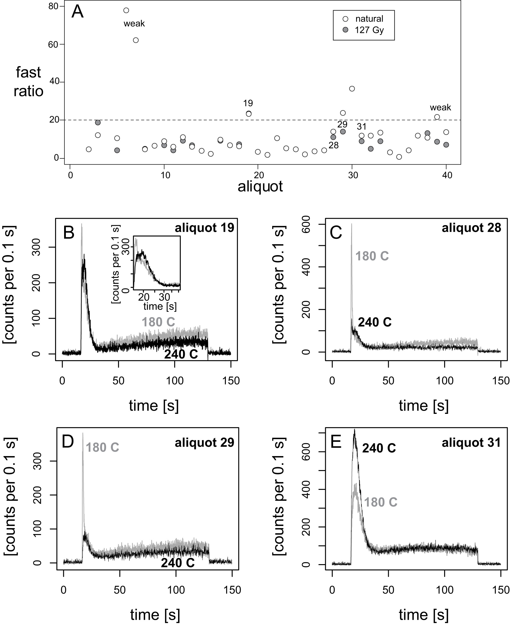
Along with selection of a rather small dataset, as mentioned earlier, some of the aliquots automatically selected by applying the FR criterion would correspond with aliquots with a weak signal or to aliquots with a presence of unstable components as detected in the LM-OSL tests (e.g., aliquot 19 or 29 in Fig. 5B and D). On the other hand, potentially acceptable aliquots with signal dominated by a fast component would not be selected (e.g., aliquot 31 shown in Fig. 5E). The LM-OSL analysis shows the presence of an ultrafast component that peaks shortly before the fast component during the LM-OSL measurement (inset in Fig. 5B). The peak representing this component is reduced upon application of the 240°C preheat step (Fig. 5C and D). Some aliquots display what we interpret as fast components based on the LM-OSL and CW-OSL decay curves (e.g., Fig. 5E). We did not perform further analysis of the LM-OSL curves, for example, determining photoionization cross-section values or deconvolution of the curves (cf. Jain et al., Reference Jain, Murray and Bøtter-Jensen2003), because results were not consistent enough between aliquots to yield a general characterization of our samples.
Based on these initial results, quartz OSL analysis in our dating experiments was performed using the following protocols: (1) all aliquots given preheat/cut heat temperatures of 240°C/220°C; (2) in a few samples, aliquots were run with an additional short (3 s) shinedown at low power (2 mW/cm2) to try to remove a potential ultrafast signal detected in the LM-OSL experiments (cf. Goble and Rittenour, Reference Goble and Rittenour2006); and conversely, (c) a less stringent preheat at 200°C/180°C was performed in a few samples to test the possible effect of the apparent ultrafast component observed in the abovementioned LM-OSL experiments. The preheat/cut heat setting at 200°C/180°C corresponds to an approach previously published for some of the samples we re-analyzed in this study (Antinao et al., Reference Antinao, Davis and Loope2023; Loope et al., Reference Loope, Antinao, Jacobs, Gray and Boulding2024) that has been used with success in dating MIS 2 deposits of northern and central Indiana (Jacobs et al., Reference Jacobs, Gray, Loope, Antinao and Rupp2023; Antinao et al., Reference Antinao, Fleming, Rupp, Brown, Karaffa, Loope and Jacobs2024; see Table 4 for details). All equivalent dose data for quartz OSL, once combined with dose-rate data to calculate an age, were compared with other geochronometers (Tables 3 and 4).
Feldspar IRSL signal properties
We tested samples from all sites for feldspar post-IR IRSL200 signal behavior (all equivalent dose distributions are shown in the Supplementary Data File). All samples display high sensitivity (Fig. 6A), and dose–response curves in general were fit with exponential interpolation, although in some cases, the use of double exponential and, rarely, exponential plus linear interpolation was needed to fit the data. Data were fit considering uncertainties, especially given that some of the samples appeared to be close to saturation. Bleaching in natural conditions was measured for sample IGWS-278. After 8 h of continuous exposure to natural sunlight, the residual post-IR IRSL200 signal is about 2% of a ∼10 Gy dose. Dose-recovery tests with a 127 Gy dose were performed on
Feldspar infrared-stimulated luminescence (IRSL) characteristic data. (A and B) Feldspar IRSL signal, both for IRSL at 50°C and post-IR IRSL at 200°C, shown for the natural dose (A) and test dose (13 Gy; B) decay curve of sample IGWS-497, aliquot 1. (C) Sensitivity-corrected luminescence signal (Lx/Tx) dose–response curves, adding natural (Ln) observation and interpolated equivalent dose value, using an exponential fit. (D) Dose–response curve showing double exponential fit. (E) Post-IR IRSL200 De distribution kernel plot for sample IGWS-451. Fading rates are displayed for individual aliquots using a color ramp (inset legend). Note the number of saturated aliquots observed and the tail of the distribution. The last recycling step for these runs was ∼1100 Gy, and values were accepted when Ln/Tn intercepts the dose–response curve within measured error. (F) Histogram plot showing distribution of g-values observed on sample IGWS-451 (same color scale as E). Fading rates represented by g-values approximately less than 1.8%/decade are within 1-sigma uncertainty of zero.
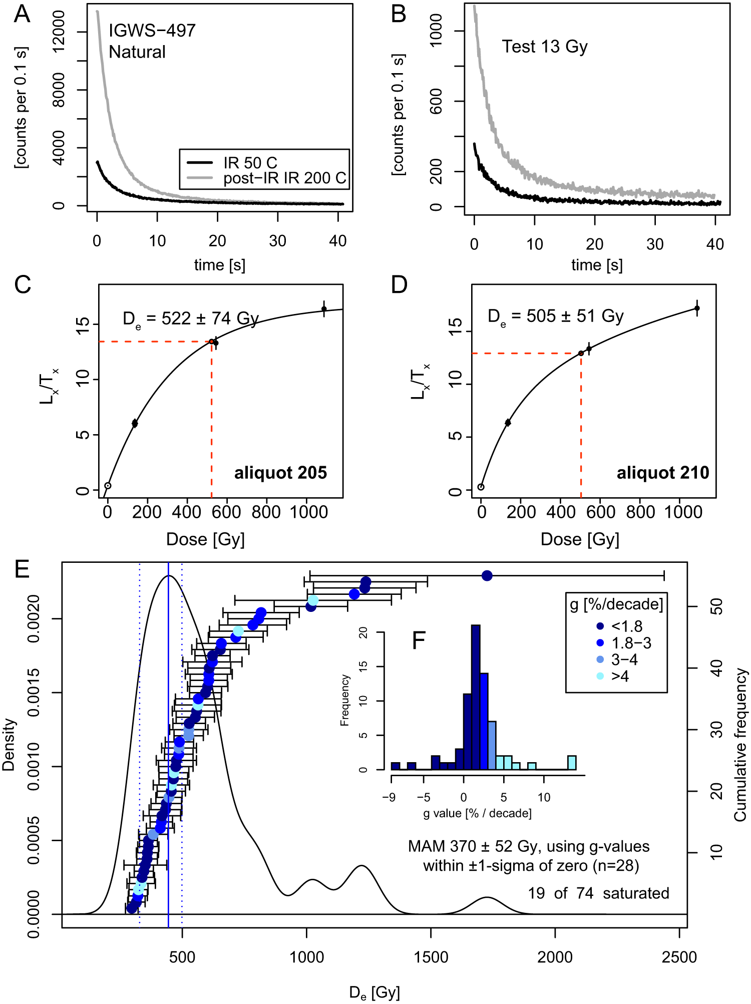
IGWS-47, IGWS-131, IGWS-278, and IGWS-452. The given dose was recovered within 5%. Recycling was within 10% in more than 95% of measured aliquots, and recuperation values were low, usually fluctuating between 0.1% and 3.4%, with a mean of 1.4% in the accepted aliquots. Fading tests on the post-IR IRSL200 signal (Supplementary Fig. SDF5-A–C) indicated g-values fluctuated between 0 (or negative in some cases) to 2% on average, although the distribution is wide (Fig. 6F). Histogram (Fig. 6F) and kernel density plots (Supplementary Fig. SDF-5D, E) of the g-value distributions show that values for aliquots with observed finite De values are clustered around 1%/decade (Supplementary Fig. SDF-5D for sample IGWS-46), and usually values of less than 1.8%/decade are within ±1-sigma of zero (vertical lines for g-value = 0 and g-value = 1.8 are in Supplementary Fig. SDF-5D for comparison with plotted data). The distribution of g-values for aliquots displaying saturated natural signal is practically identical to the distribution for the aliquots for which we could calculate finite burial doses via interpolation (Supplementary Fig. SDF-5).
All equivalent dose distribution plots are shown in Supplementary Figures SDF-7–SDF36. Individual results in the context of selected stratigraphic sections are presented in Figures 7–9 and introduced later. Summary equivalent dose data and ages and comparison with other chronometers are presented in Table 4 and Figure 10.
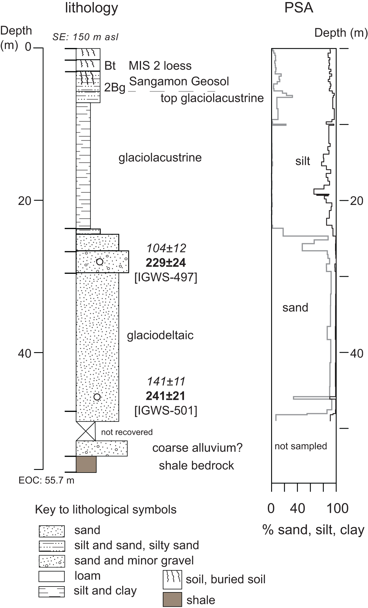
TWN-02 borehole results. (A) Lithological description and soils horizonation, including luminescence chronology (feldspar infrared-stimulated luminescence [IRSL] ages are shown in ka). (B) Particle size analysis (PSA) cumulative plot. (C) Cosmogenic depth-profile modeling results (calculated with methods by Hidy et al. [Reference Hidy, Gosse, Pederson, Mattern and Finkel2010]), with broad gray curve including results of individual Monte Carlo model runs (total 10,000 runs; the black curve indicates Bayesian best estimate). Uncertainty in the cosmogenic 10Be concentration is smaller than the size of the symbols. Model 10Be profile age depicted (145+15−18 ka at 2-sigma) corresponds to duration of exposure before loess layer deposition, which adds 25 ± 4 ka to the final age of the sediment (details in text).

Environmental dose rate
Dose-rate ancillary data, including location and depth data, are presented in Table 3. The low values measured for water content in samples IGWS-277 and IGWS-278 are thought to be caused by dewatering while coring with the open barrel. We used a value of 9 ± 4% for these and other samples in the vadose zone (see “Methods”). External dose-rate values range between ∼1.1 and ∼2.0 Gy/ka (Table 3).
Cosmogenic depth-profile dating
At the TWN-02 site, landform stabilization before deposition of MIS 3 (Roxana Loess) and MIS 2 (Peoria Loess) layers was tested with a cosmogenic 10Be depth profile (Fig. 7). A decrease in 10Be concentration with depth was observed, without major deviation from the expected pseudo-exponential profile (Hidy et al., Reference Hidy, Gosse, Pederson, Mattern and Finkel2010). The model returned uniform distributions for erosion rates, with median values around 0 cm/ka. Model inheritance estimated for the TWN-02 profile is ∼ 8 × 10⁴ atoms/g. The exposure age that estimates duration of Sangamon Geosol development was determined as  $145^{+15}_{-18}$ ka (Fig. 7). When quadrature, the estimated duration of cover of the loess layer including the postglacial soil developed on it (25 ± 4 ka), is added in, the age of glaciofluvial sediment deposition is
 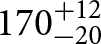 $170^{+12}_{-20}$ ka (±2-sigma; approximately 170 ± 10 ka [1-sigma]; Fig. 7).
Stratigraphy, soil data, and integrated geochronology
Luminescence geochronology for all sites is presented in the following sections, along with a description of stratigraphy and pedostratigraphy. Soil horizonation is presented for each sampled section or borehole to indicate similarities that can be used to confirm presence of a Sangamon Geosol (Jacobs et al., Reference Jacobs, Konen and Curry2009). We note that the lithostratigraphy below the loess layers and the Sangamon Geosol cannot necessarily be correlated between sites. Specific details and comparison of soil profiles are presented in Supplementary Table SDF-3.
Site 1
Borehole TWN-02 at site 1 (Fig. 7) was drilled on a dissected, flat-top glaciodeltaic and glaciolacustrine terrace (see Fig. 1, Supplementary Figs. SDF-1 and SDF-2 for details on the geomorphology at the location). Grain-size data for this borehole (Fig. 7) show about 1.5 m of silt loam with modern soil horizonation (interpreted as MIS 3 Rozana Loess and MIS 2 Peoria Loess) that accumulated over a sandy sediment with clay-rich horizons that contains soil morphology consistent with the Sangamon Geosol (cf. Jacobs et al., Reference Jacobs, Gray, Loope, Antinao and Rupp2023). The Sangamon Geosol developed at site 1 is thick (>3 m), with a well-developed Bt horizon with weak prismatic to moderate subangular blocky structure and 10YR to 7.5YR hues the Munsell color system (Supplementary Table SDF-3). At the bottom of the borehole, a laminated silty sand is prominent, which also can be found in deeper boreholes in the vicinity (cf. Loope et al., Reference Loope, Antinao, Monaghan, Autio, Curry, Grimley, Huot, Lowell, Nash and Florea2018; Supplementary Fig. SDF-2). Previous luminescence dating on sample IGWS-47 at site 1 includes a quartz OSL age of 139.9 ± 52 ka (Loope et al., Reference Loope, Antinao, Jacobs, Gray and Boulding2024), which added aliquot data to the age of 131 ± 11 ka (Loope et al, Reference Loope, Antinao, Monaghan, Autio, Curry, Grimley, Huot, Lowell, Nash and Florea2018; depicted in Fig. 1). Three samples obtained near the base of a borrow pit excavated at the edge of the terrace, a few hundred meters south of TWN-02 (Supplementary Fig. SDF-2A), yielded fading-corrected IRSL (50°C) ages on feldspar of 195 ± 14 to 216 ± 20 ka (reported in Loope et al., Reference Loope, Antinao, Monaghan, Autio, Curry, Grimley, Huot, Lowell, Nash and Florea2018, Reference Loope, Antinao, Jacobs, Gray and Boulding2024; Fig. 1). The correction used by Loope et al. (Reference Loope, Antinao, Monaghan, Autio, Curry, Grimley, Huot, Lowell, Nash and Florea2018) relied on the model of Huntley and Lamothe (Reference Huntley and Lamothe2001) which is applicable only in the linear portion of the dose–response curves for the analyzed samples, and therefore these ages are not considered in our subsequent discussion.
Quartz OSL ages of 93 ± 8 ka (IGWS-46; Table 4) and 111 ± 12 ka (IGWS-47; Table 4) were obtained (Fig. 7), while post-IR IRSL200 ages in the same samples yielded ages of 192 ± 22 ka (IGWS-46; Table 4) and 165 ± 18 ka (IGWS-47; Table 4). Quartz OSL ages for sample IGWS-46 and IGWS-47 are considerably younger than the feldspar post-IR IRSL200 ages. Both feldspar ages are within uncertainty (±1-sigma) of the sediment age calculated based on the cosmogenic depth profile (Fig. 7).
Site 2
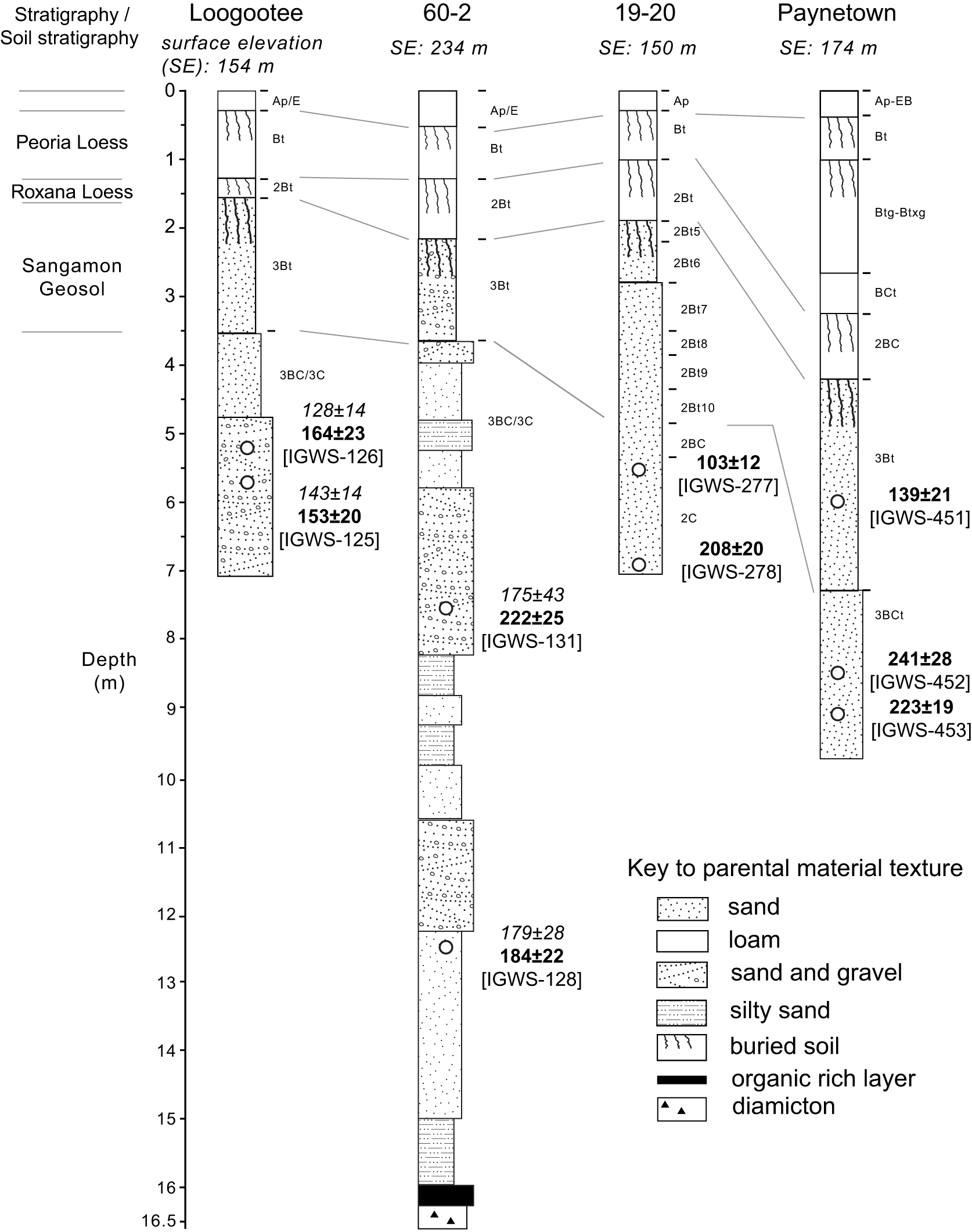
Section 60-2 at site 2 is at the proximal edge of a glaciofluvial fan, draining the MIS 6 ice margin near the present-day valley of the White River (Fig. 1, Supplementary Fig. SDF-1). Horizontal planar-bedded sandy gravel and cross-bedded sand beds (Figs. 2 and 8, Supplementary Figs. SDF-2 and 3) are exposed by erosion in a deep ravine at the ice-proximal edge of an outwash fan. The Sangamon Geosol is developed in glaciofluvial sands and is characterized by a well-developed Bt horizon with blocky and prismatic structure and hues as red as the 2.5YR (Jacobs, Reference Jacobs1994, Reference Jacobs1998; Figs. 2 and 8; Supplementary Table SDF-3). Quartz OSL ages previously reported for the section by Jacobs et al. (Reference Jacobs, Gray, Loope, Antinao and Rupp2023) of 174 ± 28 ka (IGWS-128; recalculated to 179 ± 28 ka on Table 4 using a slightly higher water content) and 175 ± 43 (IGWS-131; Table 4) are based on preheat/cut heat settings of 220°C/200°C and are within 1-sigma of each other (Fig. 8). Feldspar post-IR IRSL200 dates (this study, Table 4) of 184 ± 22 ka (IGWS-128) and 222 ± 25 ka (IGWS-131) are within 1-sigma of the quartz OSL ages.
Lithologic and soil horizonation data for sections and boreholes described in the text. Locations for all sites in Figure 1. Ages (ka) indicated at ±1-sigma: quartz optically stimulated luminescence (OSL) in italics, feldspar post-IR infrared-stimulated luminescence (IRSL) in boldface (Table 4). SE, surface elevation.
Site 3
The Loogootee section at site 3 is at a former borrow pit excavated into a major outwash terrace (Fig. 1), in a tributary to the East Fork White River valley (Supplementary Figs. SDF-1 and SDF-2). A 7-m section (Figs. 2 and 8; Supplementary Fig. SDF-3) displays sandy gravel and cross-bedded sand beds with a well-developed Sangamon Geosol profile (Supplementary Table SDF-3), covered by MIS 2 loess (Figs. 2 and 8). Quartz OSL ages of 138 ± 13 ka (IGWS-125) and 128 ± 14 ka (IGWS-126) are within 1-sigma of each other (Fig. 8). Our estimates are based on the CAM (Galbraith et al., Reference Galbraith, Roberts, Laslett, Yoshida and Olley1999) for the observed distributions (Supplementary Figs. SDF-14 and SDF-15), even considering that overdispersion is closer to 50% for both. If the MAM of Galbraith et al. (Reference Galbraith, Roberts, Laslett, Yoshida and Olley1999) had been used considering a model sigma-b parameter estimated from well-bleached aeolian samples described for IGWS-277 and IGWS-278 (Supplementary Figs. SDF-22 and SDF-23), ages close to 80 ka would have been estimated for IGWS-125 and IGWS-126, which are too young considering the stratigraphic and pedostratigraphic constraints. Feldspar post-IR IRSL200 dates of 150 ± 20 ka (IGWS-125) and 164 ± 23 ka (IGWS-126) are within 1-sigma from quartz OSL ages. Sample IGWS-125 was reported earlier by Antinao et al. (Reference Antinao, Davis and Loope2023) as 157 ± 15 ka when measured with a quartz OSL SAR protocol using preheat parameters of 200°C/180°C.
Site 4
The Paynetown borehole at site 4 was drilled on top of a high terrace east of Bloomington (Fig. 1), about 30 m above the level of the Holocene Salt Creek, now inundated by Lake Monroe (see Supplementary Fig. SDF-1 and Supplementary Fig. SDF-2 for details on the geomorphology at the location). The borehole displays about 3 m of silt loam in a distal colluvial environment, with modern soil horizonation, that accumulated over a sandy and silty-sand glaciofluvial sediment with pedogenic clay-rich horizons (Fig. 8). We interpret the clay-rich B horizon to be associated with the Sangamon Geosol (Supplementary Table SDF-3). Three samples were taken from this borehole. Sample IGWS-451 was collected in the lower portion of the Bt horizon (Fig. 8), yielding a feldspar post-IR IRSL200 age of 139 ± 21 ka, while samples near the bottom of the borehole in the BC horizon gave ages of 241 ± 28 ka (IGWS-452) and 223 ± 28 ka (IGWS-453). Quartz OSL ages are consistently lower than feldspar ages and inconsistent with the pedostratigraphic and geomorphologic setting, with estimates of 73 ± 7 ka (IGWS-451), 30 ± 9 ka (IGWS-452), and 98 ± 36 ka (IGWS-453) (Table 4). Besides the apparent age underestimation for quartz OSL data, another challenge for quartz OSL was the low yield: very few aliquots produced acceptable dose–response curves (Table 4).
Site 5
Boreholes 19-20 (site 5) and 21-39 (site 6, next section) were drilled on the relatively flat expanse related to glacial Lake Patoka (Gray, Reference Gray1988), west of Jasper (Fig. 1). Borehole 19-20 was drilled on the top of a dune. From the surface, the core displays at the top ∼1.2 m of silt loam with modern soil horizonation (Fig. 8) that accumulated as MIS 2 loess. The loess is deposited over a sandy and silty-sand sediment with clay-rich horizons representative of soil morphology associated with the Sangamon Geosol (Supplementary Table SDF-3). At 5.6 m depth, sample IGWS-277 gives a quartz OSL age of 77 ± 7 ka (Fig. 8, Table 4). A feldspar post-IR IRSL200 age for the same sample is 103 ± 12 ka (Fig. 8, Table 4). Both ages were calculated with a CAM (Galbraith et al., Reference Galbraith, Roberts, Laslett, Yoshida and Olley1999), based on low overdispersion around the CAM value, and skewness close to zero. At the bottom of the borehole, at what is considered the base of the dune, a CAM quartz OSL age of 110 ± 9 ka (IGWS-278) was obtained (Table 4). Sample IGWS-278 was previously measured using lower preheat (200°C/180°C) settings on quartz OSL by Antinao et al. (Reference Antinao, Davis and Loope2023), yielding an age of 115 ± 16 ka. The feldspar post-IR IRSL200 age for IGWS-278 is 208 ± 20 ka using a CAM estimate (Fig. 8, Table 4).
Site 6
Borehole 21-39 at site 6 reached the bottom of the basin filled by glacial Lake Patoka at 55.7 m deep (Antinao et al., Reference Antinao, Davis and Loope2023). The recovered core displays a fining upward sequence (Fig. 9), with glaciodeltaic sand buried by a silt and clay glaciolacustrine sequence that grades toward the top into a sandy silt and sand. The Sangamon Geosol is developed into the glaciolacustrine sediments (Supplementary Table SDF-3) and is covered by MIS 2 loess (Fig. 9). Quartz OSL dating at 200°C/180°C preheat/cut heat settings (Table 4), yield ages of 85 ± 8 ka (IGWS-497) and 73 ± 10 ka (IGWS-501) that are younger than ages determined with 240°C/220°C preheat/cut heat settings (104 ± 12 ka for IGWS-497, 141 ± 11 ka for IGWS-501; Table 4). An age of 151 ± 35 ka was obtained using a short-shine before the quartz OSL measurements for sample IGWS-501 (Table 4). Post-IR IRSL200 feldspar ages of 229 ± 24 ka (IGWS-497) and 241 ± 21 ka (IGWS-501) are not consistent at 1-sigma with the quartz OSL dates.
Lithologic, soil horizonation, and particle size analysis (PSA) data for borehole 21-39 (Antinao et al., Reference Antinao, Davis and Loope2023). Location shown in Figure 1. Quartz optically stimulated luminescence (OSL) ages (ka) are shown in italics, while feldspar post-IR infrared-stimulated luminescence (IRSL200) ages (ka) are shown in boldface (Table 4). SE, surface elevation; EOC, end of core. Ages (ka) indicated at ±1-sigma: quartz optically stimulated luminescence (OSL) in italics, feldspar post-IR infrared-stimulated luminescence (IRSL) in boldface.
Discussion
Luminescence properties
Quartz OSL sensitivity
The OSL decay curves for aliquots in sample IGWS-278 (Fig. 3A and B) are typical of many samples in the broader ice-marginal area characterized in this study. At least half of the aliquots selected for further investigation after observation of the first shinedown (natural) signal showed sensitivities of less than 30 counts/Gy/grain, measured in the first second of stimulation with the blue LEDs at 100 mW/cm2 after irradiation with ∼13 Gy (Fig. 3B). For comparison, the sensitivity of coarse-grained Freiberg calibration quartz (Richter et al., Reference Richter, Woda and Dornich2020) is more than 160 counts/Gy/grain. A few aliquots (Fig. 3A) showed sensitivities one or two orders of magnitude larger than the weak aliquots, suggesting that the increase in sensitivity is caused by one or two high-sensitivity grains, because there is only a 10–20% difference between the number of grains used in each aliquot, not a difference of one or two orders of magnitude (see photographs of typical aliquots in Supplementary Fig. SDF 4A–F). The observed behavior suggests that the sample is a mixture of quartz grains with a broad spread in sensitivity values.
The presence of several quartz populations has been proposed for samples derived from glaciofluvial settings (Houmark-Nielsen, Reference Houmark-Nielsen2008). Different quartz populations were related to the presence of different age sets, but not quartz with different luminescence properties. Given the broad spread in lithologic types the ice sheet might have traversed, ranging from igneous and metamorphic Precambrian rocks of the Canadian Shield to sandstones of Paleozoic sedimentary basins of the craton, it is reasonable to expect different quartz types might produce differences in the sensitivity for small aliquots for samples in this area near the MIS 6 ice margin (Fig. 1). The observed difference in sensitivity also suggests that uniquely bright aliquots might be dominated by only one grain, with implications for the success of single-grain dating in the future. Unfortunately, most bright aliquots also tend to be saturated (Fig. 3C, for example, aliquot 12, run 7, IGWS-278), with few exceptions. This effect reduces the proportion of aliquots that can yield a finite age.
Effects of quartz preheat treatment on observed ultrafast signal
Previous research on MIS 2 and a few MIS 6 aeolian and glaciofluvial sediment samples from ice-proximal settings in northern and central Indiana (Antinao et al., Reference Antinao, Davis and Loope2023, Reference Antinao, Fleming, Rupp, Brown, Karaffa, Loope and Jacobs2024; Loope et al., Reference Loope, Antinao, Monaghan, Autio, Curry, Grimley, Huot, Lowell, Nash and Florea2018, Reference Loope, Antinao, Jacobs, Gray and Boulding2024) have suggested that experimental parameters used for quartz OSL dating of MIS 2 sediments might be broadly applicable to older sediments as well. Within these parameters, for example, the use of certain preheat conditions and selection of time intervals for signal determination (use of early light subtraction vs. late light subtraction; Cunningham and Wallinga, Reference Cunningham and Wallinga2010) have been explored. Preheat plateau experiments presented here (Fig. 4) show behavior consistent with previously measured MIS 2 sample sets (Loope et al., Reference Loope, Antinao, Jacobs, Gray and Boulding2024). Ages obtained with relatively lower preheat parameter protocols (e.g., 200°C/180°C; samples IGWS 497 and IGWS-501; Table 4) however show underestimation when compared with feldspar post-IR IRSL200 data (Fig. 10, Table 4). Apparent underestimation has also been observed in samples dated to 111 ± 19 and 120 ± 17 ka by Jacobs et al. (Reference Jacobs, Gray, Loope, Antinao and Rupp2023) in core B-1 in the Flatwoods area (Fig. 1, Supplementary Fig. SDF-1), measured with similar preheat parameters.
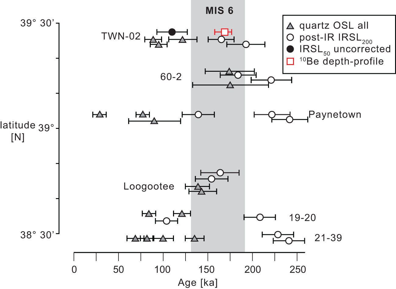
Summary of luminescence dating (quartz optically stimulated luminescence [OSL], triangles; feldspar infrared-stimulated luminescence [IRSL], circles) and cosmogenic depth-profile (square; the time for loess layer deposition is included in the depicted age, as in Figure 7) geochronologic data for the Marine Isotope Stage (MIS) 6 southwestern Indiana ice margin. Shaded area is MIS 6 (Lisiecki and Raymo, Reference Lisiecki and Raymo2005).
In the case of TWN-02, quartz ages are consistently younger than feldspar ages (Fig. 10). In other sites, ages of roughly half the expected value given the pedostratigraphic data were obtained (Paynetown data, samples IGWS-451 to IGWS-453; Fig. 10, Table 4). A few of the quartz OSL ages, measured with preheat parameters similar to those displaying underestimates, are in agreement with feldspar IRSL and soils data (e.g., Flatwoods data on 60-2 site; Jacobs et al., Reference Jacobs, Gray, Loope, Antinao and Rupp2023).
Results of our initial LM-OSL experiments at different preheat temperatures (Fig. 5) suggested that a potential ultrafast component of the measured natural doses could be decreased with higher preheat temperatures, as has been documented elsewhere (Goble and Rittenour, Reference Goble and Rittenour2006). Two samples from different sites (IGWS-47 from TWN-02, IGWS-501 from 21-39) were run with a modified protocol, adding a short-shine (3 s) at low power (2 mW/cm2) before the main blue LED stimulation. In the case of IGWS-47, the age underestimates the cosmogenic depth profile–derived age (Fig. 7) and is younger than the age derived from standard preheat protocols without a short-shine step. Sample IGWS-501 on the other side, while still displaying underestimation with respect to the feldspar, is within 1-sigma of the estimate that used only higher preheat settings (Table 4). The reduced number of aliquots accepted with observable signal compared with other protocols suggests that the stronger preheat treatment and the short-shine induced in many aliquots an undesirable loss of the weak fast component, besides the expected removal of the ultrafast signal. Without a compelling case for the effectiveness of this treatment after experiments with these two samples, we decided not to apply it to all samples.
All these observations suggest that for most of the aliquots measured for samples throughout the ice-marginal drainage system or in valley-train deposits across the, the quartz OSL signal is unreliable because (1) it mostly lacks a well-defined, easy to discriminate fast component; and (2) when a bright, fast signal is found, it is commonly field saturated and therefore any data are excluded from quantitative analysis. Presence of an unstable, ultrafast signal appearing in variable proportions that are sample-dependent and that cannot be removed without affecting the stable signal is cause for underestimation of ages obtained with quartz OSL.
Feldspar IRSL signal properties: assessment of fading
Feldspars showed high sensitivity to both IRSL stimulation at 50°C (IR50) and post-IR IRSL signal measured at 200°C (Fig. 6). When a SAR protocol was applied as an independent protocol to the IR50 signal (i.e., the SAR sequence was completed for the IR50 signal only, and not measured as part of the post-IR IRSL200 protocol in Table 1), however, the calculated age showed underestimation in sample IGWS-47 (Table 4). The effects of fading of the IR50 signal are noticeable (Supplementary Fig. SDF-12) and larger than those observed in the rest of the samples measured with post-IR IRSL200 protocols. This result is expected given previous data on feldspar IR50 signal fading across the North American continent (e.g., Huntley and Lamothe, Reference Huntley and Lamothe2001; Rice et al., Reference Rice, Ross, Paulen, Kelley, Briner, Neudorf and Lian2019).
Fading was also observed in post-IR IRSL200 data from the study area (Fig. 6), although on average more than 60% of the aliquots showed negligible fading (Table 4, see, e.g., Supplementary Fig. SDF-7 for sample IGWS-46). We considered fading rates as negligible when the g-value was within ±1-sigma uncertainty of zero (Supplementary Fig. SDF-5; in practice this was very similar to considering g-values <1.8%/decade; see Fig. 6 for an example on sample IGWS-451). A few negative fading values were obtained (Fig. 6, Fig SDF-5D); most are within ±1-sigma of zero (Supplementary Fig. SDF-5). For the rest of the negative values, it is possible that relatively low doses used for the fading test might account for this effect. Additional fading measurements in two samples were performed, with fading tests using a dose of 63 Gy instead of the standard 13 Gy mentioned in Table 2. Results do not show a significant difference in g-values or in their relative uncertainties (Supplementary Fig. SDF-40).
Uncorrected post-IR IRSL200 ages agree at ±1-sigma with the cosmogenic age at site 1 (Fig. 7), and in all sites they agree with the pedostratigraphic constraints, except for borehole 21-39 and two samples at Paynetown (Fig. 10). We are therefore confident that our choice of cutoff within ±1-sigma uncertainty of zero (Supplementary Fig. SDF-5) supports the use of uncorrected data. Our results indicate that the choice of small aliquots (Supplementary Fig. SDF-4) can adequately discriminate fading rates, avoiding the need to use average fading rates from multiple aliquots. The spread observed in fading rates is consistent with the spread observed in post-IR IRSL200 signal measured after a test dose (Supplementary Fig. SDF-39) and with the observations for the sensitivity of quartz, where differences of one to two orders of magnitude in sensitivity appear across aliquots containing roughly an average of 10–40 grains (Fig. 3). The distribution of measured g-values on aliquots displaying saturation in their natural signal compared with aliquots with a finite equivalent dose (Supplementary Fig. SDF-5) is similar and supports our choice of calculating burial dose from the sample dose distributions including only aliquots with fading rates within ±1-sigma of zero.
Data from the literature in different settings support this choice. For example, Roberts (Reference Roberts2012) and Roberts et al. (Reference Roberts, Bryant, Huws and Lamb2018) found fading rates with g-values in the order of 1–1.5%/decade for post-IR IRSL225 analysis (measured on Risø readers) but decided not to apply a fading correction. Firla et al. (Reference Firla, Luthgens, Neuhuber, Schmalfuss, Kroemer, Preusser and Fiebig2024), in a glaciofluvial context, also found g-values within uncertainty of 1%/decade for post-IR IRSL225 data, and they decided not to correct their equivalent dose data.
Effects of depositional environment and provenance on equivalent dose distributions and age estimates
Partial bleaching
Partial bleaching is evident in both quartz and feldspar data (Fig. 10, Table 4), highlighted by the skewed equivalent dose distributions and the number of aliquots with saturated luminescence signal. The effect is more clearly observed in the feldspar post-IR IRSL200 equivalent dose distributions because of the higher D 0 values observed for individual dose–response curves, which allowed recovering higher De values (e.g., samples IGWS-451, Fig. 6; IGWS-47, Supplementary Fig. SDF-9). In quartz, higher De values are masked by field saturation observed beyond ∼2D 0, as discussed in the next section. In general, our data suggest that (1) some degree of signal averaging between partially bleached and fully bleached grains is present in the small aliquots we studied, as pointed out by Thrasher et al. (Reference Thrasher, Mauz, Chiverrell and Lang2009); and (2) that within sediment packages at the scale of a single site (e.g., Paynetown; Fig. 10), partial bleaching could be highly variable.
Glaciofluvial settings are traditionally considered to be affected by partial bleaching (e.g., Houmark-Nielsen, Reference Houmark-Nielsen2008; Fuchs and Owen, Reference Fuchs and Owen2008; Thrasher et al., Reference Thrasher, Mauz, Chiverrell and Lang2009; Kalińska et al., Reference Kalińska, Alexanderson and Krievāns2020, Reference Kalińska, Weckwerth and Alexanderson2023), although studies have pointed out that bleaching can be appropriately achieved in this setting (Thomas et al., Reference Thomas, Murray, Kjær, Funder and Larsen2006). The effect has been considered to decrease with increasing transport distance from the ice margin, especially in valley-train outwash and in glaciodeltaic settings (e.g., Gaar et al., Reference Gaar, Lowick and Preusser2014; Curry et al., Reference Curry, Kehew, Antinao, Esch, Huot, Caron and Thomason2021; Erber et al., Reference Erber, Kehew, Schaetzl, Gillespie, Sultan, Esch, Yelich, Curry, Huot and Abotalib2023; Brookfield et al., Reference Brookfield, J.P and Murray2024).
Our feldspar data show mixed results. Some of our dates from sites along glaciofluvial valley-train tracks (Loogootee and Paynetown; Fig. 1) are consistent at ±1-sigma with aeolian (site 19-20) and glaciodeltaic (TWN-02) sediments (Fig. 10). In our coupled test site (TWN-02 borehole), post-IR IRSL200 ages are within 1-sigma uncertainty of each other and within 1-sigma of the 10Be age (Fig. 10). In this case, even sediments deposited in proglacial fans or deltas might have experienced enough sediment bleaching of the observed luminescence signal to properly account for the age. A similar result was obtained by Brookfield et al. (Reference Brookfield, J.P and Murray2024) for the MIS 2 LIS margin in Ontario, Canada.
On the other side, sample IGWS-451 and adjacent samples in the Paynetown borehole (Fig. 10)—also in a valley-train setting and more than 50 km away from the ice margin (Fig. 1)—display partial bleaching as determined by overdispersion values and the skewness of their distributions (Fig. 6). MAM ages calculated for two of them are outside the expected range based on soil development (Fig. 10). The glaciodeltaic sediments at borehole 21-39 also show ages that are not consistent at 1-sigma with MIS 6 deposition (Fig. 10). At face value, sedimentation here could have occurred during the MIS 7 interglacial (∼240–190 ka). However, given the glacial geomorphology and soil stratigraphy at these sites (Figs. 8 and 9, Supplementary Figs. SDF-1 and SDF-2), we consider these are examples of partial bleaching during glaciofluvial and glaciodeltaic deposition, which has been documented at relatively long distances from the ice margin in similar settings around the world (e.g., Kalińska et al., Reference Kalińska, Alexanderson and Krievāns2020, Reference Kalińska, Weckwerth and Alexanderson2023). The high sensitivity displayed by feldspars across all our analyzed samples (Fig. 6) highlights the potential for addressing partial bleaching in this environment with single-grain dating.
Influence of quartz luminescence properties on observed dose distribution
Quartz provenance affects luminescence properties and therefore dispersion of observed doses (Sawakuchi et al. Reference Sawakuchi, Blair, DeWitt, Faleiros, Hyppolito and Guedes2011, Reference Sawakuchi, Jain, Minelli, Nogeuira, Bertassoli, Haeggi and Sawakuchi2018; Del Río et al., Reference Del Río, Sawakuchi, Góes, Holanda, Furukawa, Porat, Jain, Minelli and Negri2021). Observed quartz OSL decay curves display a mixture of fast, slow, and medium components in aliquots within all samples analyzed in this study (Fig. 3). Some of the broad variation in signal character and intensity from quartz within the glaciofluvial sediments in the MIS 6 margin might arise from variable contribution of sand directly eroded from the Mississippian–Pennsylvanian belt of sandstones that are within and adjacent to the study area, combined with the variety of quartz sources available further north. A less marked local effect should be expected for the feldspars’ provenance, mostly derived from the Canadian Shield, hundreds of kilometers north of the study area.
A previously unreported ultrafast signal in the quartz delivered by the glaciofluvial streams in MIS 6 sediments in this region is observed (Fig. 5). Presence of this thermally unstable signal component produces age underestimation unless some modification of the signal is made (Fig. 10). Our analysis, however, returned conflicting results. In the case of sample IGWS-47 (Table 4), a more stringent preheat with a short-shine protocol before standard SAR measurements yields an age closer to the feldspar age and to morpho- and pedostratigraphic constraints, while in the case of sample IGWS-501, the opposite result was obtained. Glaciofluvial sediments studied previously with quartz OSL dating in the immediate region have not recognized this unstable signal either in MIS 2 (e.g., Loope et al., Reference Loope, Antinao, Monaghan, Autio, Curry, Grimley, Huot, Lowell, Nash and Florea2018) or MIS 6 sediments (e.g., Wood et al. Reference Wood, Forman, Pierson and Gomez2010).
A few of the quartz OSL ages obtained in glaciofluvial settings in the study area (for example, IGWS-125 and IGWS-126) indicate that the CAM model (Galbraith et al., Reference Galbraith, Roberts, Laslett, Yoshida and Olley1999) can provide a robust equivalent dose estimate. Usually, this is an indication of sediments that were well-bleached at deposition, as mentioned earlier. Data like these warrant care in their interpretation, however, as the presence of the unstable ultrafast signal mentioned earlier can combine with two additional factors to generate distributions that appear to be suitable for CAM model application without the aliquots being well bleached at burial. The main factor is the presence of relatively low D 0 values (Supplementary Fig. SDF-38) compared with the expected population De values. Low D 0 values will make a large set of aliquots to be field saturated and therefore without representation on De distribution plots. The distributions will be truncated yet still yield a statistic if many aliquots are observed. This effect has been observed before in glaciofluvial sediments in North America (Demuro et al., Reference Demuro, Froese, Arnold and Roberts2012). A second, less relevant factor is related to the higher uncertainties associated with dim signals in quartz, commonly observed in samples from this and other glaciated regions (e.g., Thomas et al., Reference Thomas, Murray, Kjær, Funder and Larsen2006; Fig. 3). Dim signals might yield reduced overdispersion compared with samples with consistently high sensitivity.
Anomalous fading effects in feldspar post-IR IR200 dose distributions
In relation to fading potentially affecting feldspar post-IR IR200 ages, we opted for using uncorrected aliquot data when fading rates were close to zero. An alternative decision to calculate ages is to calculate an individual fading aliquot correction. This could have been accomplished by applying the model of Huntley (Reference Huntley2006) and analyzing fading measurements with the algorithm of Kars et al. (Reference Kars, Wallinga and Cohen2008). Age distributions could be modeled afterward using corrected age values for individual aliquots. We tested this approach for sample IGWS-47 and found that the MAM model age using corrected data is within 1-sigma of the age determined with uncorrected data. When considering inter-aliquot variation in fading properties (e.g,, Supplementary Figs. SDF-6 and SDF-40), our data support the use of single-aliquot uncorrected post-IR IRSL200 signal in the ice-marginal environment studied.
Overdispersion
The choice of parameter sigma-b in the MAM model (Galbraith et al., Reference Galbraith, Roberts, Laslett, Yoshida and Olley1999) is critical to determine the age in this environment that is prone to partial bleaching. We estimated this parameter using the measured overdispersion for both quartz and feldspar in samples considered to be well-bleached aeolian sediment at borehole 19-20 (Fig. 8). The De distributions on both feldspar IRSL and quartz OSL data yield distributions with low skewness and overdispersion values between 17% and 34%. Similar overdispersion values are not rare in the ice-marginal settings in the broader region north of the study area (e.g., 23% in quartz OSL measurements reported for aeolian deposits in Antinao et al. [Reference Antinao, Fleming, Rupp, Brown, Karaffa, Loope and Jacobs2024]). Proximal aeolian deposition in this area with minimal transport distance after sudden drainage of glacial Lake Patoka (Antinao et al., Reference Antinao, Davis and Loope2023) could also account for the slightly skewed distribution and relatively high overdispersion in both quartz and feldspar data of the upper sample (IGWS-277; Fig. 8, Table 4). The lowermost values (25% and 17%) were used in our MAM models as sigma-b values for quartz and feldspar analysis, respectively.
Effects of depositional environment and provenance on dosimetry
Some of the samples in this study were taken in BC, BCt, and Bt horizons (Figs. 7 and 8), with minor mobilization (and leaching) of carbonates (and associated U) and deposition of iron oxides and clays being translocated to lower horizons, which in part could modify environmental dose rates. Our overall sampling scheme, however, tried to be broad enough to encompass C horizons and sediments at deeply buried levels (e.g., in borehole 21-39 and the sections at site 60-2 and Loogootee; Fig. 1). Given the broad agreement between most of the feldspar post-IR IRSL200 ages (Fig. 10), we are confident that dose rates are representative of long-term conditions. We acknowledge, however, that caution must be taken when assessing ages for these older sediments in the temperate climate of the region, and comparison of dose-rate values in pedogenic horizons with unoxidized C horizons is warranted. For the quartz data, K and U remobilization in the lower B horizons could contribute to overdispersion in burial dose distributions through microdosimetric effects (e.g., Smedley et al., Reference Smedley, Duller, Rufer and Utley2020).
For the feldspar data, the spread we observe in equivalent dose distributions might also be caused by uncertainties related to the feldspar K content in each grain, which determines the internal dose rate, and by extension affects the total environmental dose rate. It is possible that the K content in the analyzed feldspars is higher or more variable than originally estimated (10 ± 2%; Smedley et al., Reference Smedley, Duller, Pearce and Roberts2012). Although there is no reason to choose a different value for these small-aliquot multigrain measurements, we can only speculate at this point that K content might be on the higher end of the possible values based only on the fact that sensitivity is relatively high (Rhodes, Reference Rhodes2015; Fig. 6), although Smedley et al. (Reference Smedley, Duller, Pearce and Roberts2012) and Maßon et al. (Reference Maßon, Riedesel, Zander, Sontag-González and Reimann2024) have found no relationship between K content and signal intensity. If a higher K content can be demonstrated, internal dose rates, and by extension environmental dose rates, might be higher, which will result in younger post-IR IRSL200 ages.
Potential for dating older sediments
Feldspar post-IR IRSL200 dating methods discussed here show strong potential for dating glaciofluvial and glaciodeltaic deposits of pre-MIS 6 glaciations in borehole or outcrop. Given the saturation levels shown by our tests, doses of up to 800–1000 Gy (Fig. 6) could be resolved, extending the technique application well into MIS 10. Quartz OSL dating on glaciofluvial sediments, on the other hand, is not considered a good candidate because of signal instability and expected saturation (e.g., Figs. 3 and 5; Supplementary Fig. SDF-37). For example, based on obtained dose rates in Table 3 and expected age of sediments for site 1 (∼170 ka), total doses of ∼ 340–390 Gy are expected for MIS 6 sediments. As discussed earlier, dose–response curves for most aliquots display 2D 0 values below 250 Gy (Supplementary Fig. SDF-38), and therefore, even if stable quartz OSL signals used in standard SAR protocols are found in sediments older than MIS 6, samples will show field saturation. The use of techniques that extend the usual range for luminescence dating, such as thermally transferred OSL (TT-OSL; e.g., Brown and Forman, Reference Brown and Forman2012) in well-bleached quartz-rich fine-grained sediments in MIS 6 and older loess sediments could be investigated in central and southwestern Indiana to overcome the field saturation problem. Older loess exposures in the region, however, are fragmentary. Loess deposits identified in observed sections are thin (<2 m; Loope et al., Reference Loope, Antinao, Monaghan, Autio, Curry, Grimley, Huot, Lowell, Nash and Florea2018) and affected by pedogenesis in deeply structured Bt horizons where translocation might have changed dose rates significantly over time.
The partial bleaching apparent in post-IR IRSL200 feldspar ages older than MIS 6 (e.g., Paynetown, 21-39 sites in Fig. 10) is consistent with the slower bleaching of the post-IR IRSL200 signal with respect to the quartz OSL fast component documented here and elsewhere (Buylaert et al., Reference Buylaert, Jain, Murray, Thomsen, Thiel and Sohbati2012) and with deposition in glaciofluvial and glaciodeltaic settings along the margin of an ice sheet. Age overestimation generated by this partial bleaching effect could be as high as ∼50 ka (Fig. 10). However, the high sensitivity of the feldspar post-IR IR200 signal (Fig. 6) suggests that single-grain luminescence dating in these sediments could considerably reduce this overestimation.
The critical role of pedostratigraphic data
A critical element to consider is the pedostratigraphic evidence of an MIS 6 age for these sediments. All our sampling sites display the Sangamon Geosol covered by MIS 2–3 loess (Figs. 2 and 7–9, Supplementary Fig. SDF-2, Supplementary Table SDF-3). Research in the Flatwoods area (site 60-2; Jacobs, Reference Jacobs1994, Reference Jacobs1998) and in the overall Midwest region (Jacobs et al., Reference Jacobs, Konen and Curry2009, Reference Jacobs, Gray, Loope, Antinao and Rupp2023) indicates that the thickness of the B horizon and the degree of soil development are distinctive of soil development for at least ∼50,000 years during a single interglacial period (e.g., Grimley et al., Reference Grimley, Follmer, Hughes and Solheid2003; Supplementary Table SDF-3). This result stands despite local variation because of variability in drainage in the different environments where the geosol developed, which generates changes in color and structure (Jacobs et al., Reference Jacobs, Konen and Curry2009, Reference Jacobs, Gray, Loope, Antinao and Rupp2023). Soil properties for the geosol are similar to those observed in Illinois, where the Sangamon Geosol has been described (Follmer, Reference Follmer and Porter1983) and are very different from the next older soil documented in the Midwest, the Yarmouth Geosol, developed across ∼180,000 years (e.g., Grimley et al., Reference Grimley, Follmer, Hughes and Solheid2003; Supplementary Table SDF-3). All soil profiles described in sections and boreholes (Figs. 7–9, Supplementary Table SDF-3) document complete pedogenic horizon development, without truncation. Validation of the use of the Sangamon Geosol as a direct indicator for landform stability since the end of MIS 6 is also supported by data on glaciofluvial sequences from Illinois that display the Sangamon Geosol on top of sediments dated with quartz OSL. The Sangamon Geosol developed after sediment deposition at 153 ± 19 ka and 147 ± 18 ka in southern Illinois (Webb et al., Reference Webb, Grimley, Phillips and Fouke2012), 150 ± 11 ka to 128 ± 1 ka in northern Illinois (Berg et al., Reference Berg, McKay and Goble2013), and in a range from 185 ± 16 and 190 ± 16 ka toward the base and 142.7 ± 15.5 and 150.6 ± 12.6 ka toward the top of the MIS 6 glaciofluvial ancestral Mississippi River valley infill in central Illinois (Berg et al., Reference Berg, McKay and Stiff2012). This evidence is also consistent with amino acid racemization data in loess sediments capped by the Sangamon Geosol in Illinois, dating MIS 6 loess deposition to ca. 160 to 135 ka (Grimley and Oches, Reference Grimley and Oches2015).
Implications for ice-sheet activity along the MIS 6 LIS margin
We have dated several sites along the ice-marginal domain that was active during a pre-MIS 2 glaciation in southwestern Indiana. Our feldspar post-IR IRSL200 and cosmogenic 10Be profile chronologic data point to all features forming during the period broadly encompassing MIS 6 (190–131 ka). We interpret the older (>190 ka) post-IR IRSL200 ages in the set (Fig. 10, Table 4) as affected by partial bleaching based on the observed fraction of saturated aliquots and the overdispersion and positive skewness of their equivalent dose distributions.
The Paynetown and 21-39 sites display the largest apparent overestimation. Although 21-39 is a proximal glaciodeltaic site (Figs. 1 and 9, Supplementary Figs. SDF-2 and SDF-3) where partial bleaching is expected, the Paynetown site is situated along a valley-train path ∼50 km from the edge of the ice margin toward the north (Fig. 1). Two of the feldspar ages seem to be affected by severe partial bleaching (IGWS-452, IGWS-453; Table 4), even at this relatively large distance from the probable ice margin. One complicating factor is that the total amount of soil developed on this glaciofluvial terrace is thicker at Paynetown compared with other sites (Fig. 8). This factor could indicate that the glaciofluvial valley-train deposit was formed before other ice-marginal features in the region. We instead interpret the thicker soil there as sourced by additional accretion of colluvium since MIS 6 sedimentation, thanks to the position of the borehole closer to lateral hillslopes (Supplementary Figs. SDF-1 and SDF-2) than, for example, the TWN-02 or Loogootee sites (Supplementary Fig. SDF-1). Our data at Paynetown are consistent with conclusions by Kalińska et al. (Reference Kalińska, Weckwerth, Alexanderson, Piotrowski and Wysota2025), on the lack of a relation between transport distance or sedimentology to bleaching of luminescence signals in similar ice-marginal settings.
We conclude that no glacial sedimentation older than MIS 6 was documented in the sediments studied within reasonable uncertainties. Our full dataset confirms preliminary dating conducted on sites reported by Antinao et al. (Reference Antinao, Davis and Loope2023), Jacobs et al. (Reference Jacobs, Gray, Loope, Antinao and Rupp2023), and Loope et al. (Reference Loope, Antinao, Jacobs, Gray and Boulding2024). Combining our results with ages obtained by Wood et al. (Reference Wood, Forman, Pierson and Gomez2010) (Fig. 1), we conclude that the maximum extent of ice in the area during MIS 6 was reached relatively early, between 190 and 155 ka (Fig. 10). Subsequent stagnation and stability around the margin generated landforms such as fans as well as drainage changes (Jacobs et al., Reference Jacobs, Gray, Loope, Antinao and Rupp2023) until the ice margin started retreat after ∼164–153 ka, marked by the ages at Loogootee that indicate sedimentation in a valley-train outwash channel. An age of ∼135 ka on glacial Lake Quincy sediments (Wood et al., Reference Wood, Forman, Pierson and Gomez2010), northwest of the sites of this study and inboard of the maximum MIS 6 ice margin (Fig. 10), suggests the ice margin retreated north of the White River corridor at that time.
Our dataset cannot be used to identify distinctive short-term fluctuations of the ice margin within MIS 6 given the relatively high uncertainties. The lack of clear crosscutting relationships and stratigraphic preservation in the highly fragmented MIS 6 geomorphology of southwestern Indiana is also a major factor that impairs our ability to understand the short-term ice dynamics within MIS 6. Use of methods such as single-grain luminescence dating that can simultaneously help with addressing partial bleaching, along with minimizing uncertainties in K content for the feldspar used in dating (e.g., Maßon et al., Reference Maßon, Riedesel, Zander, Sontag-González and Reimann2024), can help overcome these difficulties, given the results presented here.
Conclusions
Small-aliquot luminescence analysis is suitable for determining the absolute age of glacially derived sediments along the southern MIS 6 LIS margin. Major identified problems are partial bleaching, the presence of unstable luminescence signals on quartz, and the presence of anomalous fading in feldspars. Partial bleaching of the luminescence signal affects the quartz OSL and feldspar post-IR IRSL200 ages for many of the samples, without a clear control by geomorphic setting or distance to the ice margin.
Quartz OSL ages determined using standard SAR protocols for the glaciofluvial and glaciodeltaic sediments in the region underestimate age by a considerable amount (up to 50%) when compared with stratigraphic and feldspar post-IR IRSL200 data (Fig. 10). The unreliability of quartz results can be attributed to two main factors.
First, a substantial number of analyzed aliquots lack stable OSL signal components that can be deconvolved using a simple protocol. The observed fast signal component was dim and usually tightly coupled with an ultrafast signal component. The pool of aliquots was reduced, as many of them show dominant medium and slow components that are harder to bleach. Attempts to remove unstable, ultrafast components eroded most of the fast component on analyzed aliquots. Quartz OSL ages consistent with IRSL feldspar ages and the morpho- and pedostratigraphy were obtained for one site by using modified preheat protocols, but the same procedures did not produce consistent ages in other sites.
Second, when stable quartz OSL signals can be identified in individual aliquots, they mostly display field saturation at the expected burial doses based on the lithological composition of the sediment. We conclude that quartz OSL results are erratic and unreliable, in the context of a time-consuming, sample-dependent process, and that quartz OSL dating for MIS 6 and older glaciofluvial sediments in this region should be carefully considered and always coupled to other chronometers.
Contrasting with the results for quartz, feldspar post-IR IRSL200 protocols appear to be more consistent across all sites with the stratigraphic control. At our control site, feldspar post-IR IRSL200 ages display ages that are consistent at 1-sigma to independent cosmogenic 10Be depth-profile dating, and to other stratigraphic and pedostratigraphic constraints.
Feldspar post-IR IRSL200 fading rates determined for individual aliquots allowed discrimination of a non-fading dataset in which 30% to 50% of measured aliquots were selected to calculate ages. Feldspar post-IR IRSL200 ages calculated this way range from 103 ± 12 to 241 ± 28 ka for sediments in the MIS 6 ice-marginal system. As mentioned earlier, older ages can be attributed to partial bleaching of the luminescence signal and not to the presence of sediments deposited during a glaciation older than MIS 6, considering calculated uncertainties and pedostratigraphic data. The new luminescence and cosmogenic nuclide depth-profile ages provide confirmation of interglacial-scale pedogenesis associated with the Sangamon Geosol.
While ages obtained using post-IR IRSL200 protocols on feldspar are affected by partial bleaching and anomalous fading, these factors can be accounted for using protocols such as those highlighted in this study and with single-grain analysis in future studies. Feldspar post-IR IRSL200 ages therefore represent a viable option to study glaciofluvial sedimentation of MIS 6 and older glaciations in the region.
Supplementary material
The supplementary material for this article can be found at https://doi.org/10.1017/qua.2026.10083.
Acknowledgments
Sebastien Huot (Illinois State Geological Survey) was the first to call our attention to the two-step practical protocol used here with small aliquots, to deal with dim signals in quartz found in the glacial sediments of the area. Elizabeth Moore, Valerie Beckham-Feller, and Garrett Marietta (IGWS) processed all luminescence samples. Brad Sion and Janelle Bustarde carried out cosmogenic 10Be preparation procedures at the Desert Research Institute. Alan Hidy supervised sample measurements at Lawrence Livermore National Laboratory. This research was partially funded by the Great Lakes Geologic Mapping Coalition, part of the U.S. National Cooperative Mapping Program through Cooperative Agreement No. G19AC00321. Funding for cosmogenic dating was provided as part of the Bloomington Quadrangle mapping project, part of the STATEMAP program, U.S. National Cooperative Mapping Program through Cooperative Agreement Number G22AC00424. Senior editor Nick Lancaster, guest editors Shannon Mahan and Amanda Keen Zebert, Olav Lian, and an anonymous reviewer provided detailed critical comments that greatly improved the article.


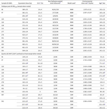


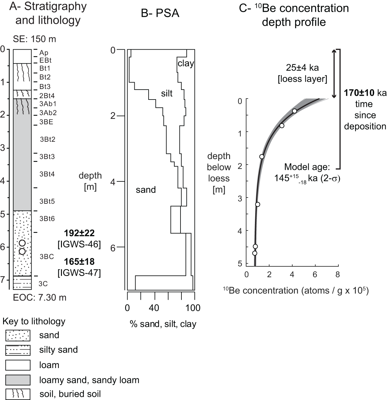


 Open access