


1. Introduction
Understanding hypersonic laminar–turbulent transition is crucial in order to develop reliable transition prediction methods. The transition process has a profound impact on the skin-friction distribution and heat loads that high-speed vehicles experience during flight. A thorough understanding of the underlying mechanisms that ultimately lead to the breakdown to turbulence is also necessary in order to design and safely operate such vehicles and to explore potential flow control strategies. Active or passive flow control strategies (for classification see, for example, Kral Reference Kral2000) can be employed to either delay or accelerate transition, depending on the application. From the well-known ‘Morkovin roadmap’ (Morkovin, Reshotko & Herbert Reference Morkovin, Reshotko and Herbert1994) of the various paths to transition, it becomes clear that flow control strategies can be targeted towards manipulation of different stages of the transition process. The path to transition depends largely on the free-stream disturbance level. For quiet tunnel conditions with a low level of free-stream turbulence, such as for the Boeing/Air Force Office of Scientific Research (AFOSR) Mach 6 Quiet Tunnel (BAM6QT) at Purdue University, experiments indicate that transition follows what Morkovin et al. (Reference Morkovin, Reshotko and Herbert1994) called path ‘a’ (environmental disturbances  $\rightarrow$ receptivity $\rightarrow$ primary instability $\rightarrow$ secondary instability $\rightarrow$ breakdown $\rightarrow$ turbulence). This means that in quiet tunnel conditions manipulation or modification of the receptivity, the primary or secondary instability or the breakdown stage could have the potential to control or delay transition to turbulence and its associated detrimental effects. These stages continuously blend into one another and have no clear distinct boundaries; consequently, the control strategies can be developed to manipulate either linear or nonlinear processes that are known to be relevant for transition.
Past research efforts on flow control in high-speed boundary layers were focused on how linear mechanisms are affected by roughness elements. Marxen & Iaccarino (Reference Marxen and Iaccarino2008) and Duan, Wang & Zhong (Reference Duan, Wang and Zhong2010) showed that two-dimensional roughness elements are capable of damping a wide range of linearly amplified frequencies while strongly amplifying another frequency band for flat plates at Mach number  $M=4.8$ and $M=5.92$, respectively. Numerical investigations for a flat plate at $M=6$ by Duan, Wang & Zhong (Reference Duan, Wang and Zhong2013) and Fong, Wang & Zhong (Reference Fong, Wang and Zhong2012, Reference Fong, Wang and Zhong2014) showed that if a 2-D roughness element has a stabilizing or destabilizing effect depends on the location of the roughness element relative to the synchronization point (synchronization between fast and slow mode, see Fedorov & Khokhlov Reference Fedorov and Khokhlov2001). In addition, Fong et al. (Reference Fong, Wang and Zhong2014) observed a compounding stabilizing effect when using two roughness elements instead of one. In experiments for a flared cone at $M=6$ at the BAM6QT (Fong et al. Reference Fong, Wang, Huang, Zhong, McKiernan, Fisher and Schneider2015), it was observed that the hot streak development on the surface of the flared cone was delayed when applying multiple (axisymmetric) roughness elements. Another method of transition delay by using so-called ‘vortex generators’ was numerically investigated by Paredes, Choudhari & Li (Reference Paredes, Choudhari and Li2018) for a $7^\circ$ half-angle cone at $M=5.3$. The vortex generators induced streaks that reduced the peak amplification rates of the boundary layer instabilities and could therefore potentially delay transition.
Numerical investigations of laminar–turbulent transition for a flared cone at  $M=6$ (Hader & Fasel Reference Hader and Fasel2018, Reference Hader and Fasel2019, Reference Hader, Fasel, Sherwin, Schmid and Wu2022) provided strong evidence that the streamwise hot streaks that arise on the surface of the flared cone in the BAM6QT experiments (see Chynoweth et al. Reference Chynoweth, Schneider, Hader, Fasel, Batista, Kuehl, Juliano and Wheaton2019) are nonlinearly generated by the nonlinear interaction of the primary and secondary disturbance waves of a so-called fundamental resonance. Hader & Fasel (Reference Hader and Fasel2021a) proposed using steady blowing and suction strips at the wall to delay the hot streak development and consequently also transition by addressing the responsible nonlinear interactions (namely the so-called fundamental resonance) for a flared cone at $M=6$. The flow control strategy employing steady blowing and suction (control) strips (Hader & Fasel Reference Hader and Fasel2021a) is based on the idea that these control strips provide axisymmetric ‘fluidic barriers’ that prevent or delay the hot streak development, and therefore transition, by hindering the steady streamwise modes from evolving. The steady blowing/suction strips significantly reduced the N-factors of the secondary disturbance waves after (fundamental) resonance onset and therefore delayed the hot streak development and subsequent transition (Hader & Fasel Reference Hader and Fasel2021a) when transition was initiated by a controlled disturbance input. The steady blowing/suction strips still led to a reduction of the N-factors of the secondary waves even when placed upstream of the synchronization location of the most amplified axisymmetric (primary) second-mode wave. In the present paper, the efficacy of this control method (steady blowing/suction strips) was investigated for a natural transition scenario.
2. Geometry and flow conditions
For the numerical investigations of the flow control strategy presented here, the same flared cone geometry, schematically shown in figure 1, as in the experiments at the BAM6QT at Purdue University (Chynoweth et al. Reference Chynoweth, Schneider, Hader, Fasel, Batista, Kuehl, Juliano and Wheaton2019) and in the natural transition simulations by Hader & Fasel (Reference Hader and Fasel2018), was used. The flared cone has a nose radius of  $r_{{nose}}=101.6\,\mathrm {\mu }\text {m}$, an initial half-angle of $\theta _{{cone}} = 1.4^\circ$, a flare radius of $r_{{flare}}=3\, {\rm m}$ and a length of $L_{{cone}}=0.51\, {\rm m}$. The flared cone model was specifically designed to enhance the N-factors due to second-mode waves, thus facilitating detailed study of second-mode dominated transition scenarios. It has been extensively studied, both experimentally and numerically, resulting in a thorough understanding of the relevant transition mechanisms (e.g. Chynoweth et al. Reference Chynoweth, Schneider, Hader, Fasel, Batista, Kuehl, Juliano and Wheaton2019). The flow control strategy presented here is tailored towards second-mode dominated transition scenarios, and therefore the flared cone model was chosen. However, for other geometries and flow conditions, where the dominant transition mechanisms may differ (e.g. first-mode or cross-flow), the flow control strategies would need to be specifically adapted. The flow conditions for the results in this paper are those of the numerical investigations by Hader & Fasel (Reference Hader and Fasel2018) without flow control. These conditions are based on the experiments at the BAM6QT (Chynoweth et al. Reference Chynoweth, Schneider, Hader, Fasel, Batista, Kuehl, Juliano and Wheaton2019) with a Mach number of $M = 6$, a stagnation temperature of $T_0=420\,{\rm K}$ and a unit Reynolds number of $Re_1=10.82\times 10^6\, {\rm m}^{-1}$. The fluid is assumed to be a calorically perfect gas with the properties of air (heat capacity ratio $\gamma = 1.4$, specific gas constant $R_{{gas}}=287.15\,{{{\rm J}}}\,({{{\rm kg}\,{\rm K}}})^{-1}$, Prandtl number $Pr=0.71$). The viscosity is calculated using Sutherland's law (Sutherland Reference Sutherland1893).

Figure 1. Schematic of the flared cone geometry.
3. Flow control strategy
The present study follows, whenever applicable, the approach suggested by Kral (Reference Kral2000): first, by specifying a control objective, identifying the flow phenomenon to be controlled, selecting an appropriate actuation strategy, and finally determining the control parameters. The control objective for the present numerical investigation becomes apparent by consulting the Stanton number  $(C_h)$ contours obtained from temperature sensitive paint (TSP) images from the experiments carried out at the BAM6QT facility for $\kern 1.5pt p_0=137.5$ psi, where $p_{0}$ is stagnation pressure, $T_0=408$ K, $Re_1=11.2\times 10^6\, {\rm m}^{-1}$ (Chynoweth et al. Reference Chynoweth, Schneider, Hader, Fasel, Batista, Kuehl, Juliano and Wheaton2019) and the time-averaged Stanton number contours obtained from natural transition direct numerical simulations (DNS) (Hader & Fasel Reference Hader and Fasel2018) as provided in figure 2(a). For both, the experiments and DNS patterns of hot streaks appearing (‘primary’ streaks), disappearing and reappearing farther downstream (‘secondary’ streaks) have been observed on the surface of the flared cone. The streamwise hot streaks lead to local ‘overshoots’ of the Stanton number exceeding the turbulent values (see figure 2b). The results provided in figure 2(b) also indicate that there is a connection between the large amplitude pressure fluctuations ( $\kern 1.5pt p'/p_{{mean}}$) on the surface of the cone and the Stanton number overshoots (hot streaks). Here $p'$ refers to the pressure disturbance relative to the laminar base flow and $p_{mean}$ is the pressure of the steady laminar base (mean) flow. Thus, for the present investigations, the flow control objective is to delay/prevent the development of the hot streaks and the detrimental effects associated with it (i.e. Stanton number overshoots and the large pressure amplitudes, see figure 2b).

Figure 2. Stanton number  $(C_h)$ contours obtained from experiments ( $p_0=137.5$ psi, $T_0=408$ K, $Re_1=11.2\times 10^6\, {\rm m}^{-1}$ Chynoweth et al. Reference Chynoweth, Schneider, Hader, Fasel, Batista, Kuehl, Juliano and Wheaton2019) using TSP and the time-averaged Stanton number from a natural transition DNS (a). Stanton number development in the downstream direction extracted along a hot streak and the development of power spectral density (PSD) amplitudes of the pressure disturbance (b). The blue squares indicate the sensor locations and the vertical dashed lines highlight the distance between two sensors in the experiments.
To control the hot streak development a thorough understanding of the underlying physical mechanisms leading to the streak formation is required. Detailed investigations of laminar–turbulent transition for a flared cone at  $M = 6$ (Hader & Fasel Reference Hader and Fasel2018, Reference Hader and Fasel2019, Reference Hader, Fasel, Sherwin, Schmid and Wu2022) had provided strong evidence that the streamwise hot streaks that arise on the surface of the flared cone in the BAM6QT experiments (Chynoweth et al. Reference Chynoweth, Schneider, Hader, Fasel, Batista, Kuehl, Juliano and Wheaton2019) are nonlinearly generated by a so-called fundamental resonance (Herbert Reference Herbert1988) namely an interaction of a large (finite) amplitude axisymmetric second-mode disturbance wave and a pair of low-amplitude oblique disturbance waves with the same frequency (fundamental resonance). Using the nonlinear interaction model described in Hader & Fasel (Reference Hader and Fasel2021b), this interaction can be written as $(f,0) - (f,\pm k_c) = (0,\pm k_c)$, where $f$ is the frequency of the dominant axisymmetric second-mode wave and $k_c$ is the azimuthal wavenumber of the secondary disturbance wave leading to the strongest fundamental resonance. Thus, the mechanism to be controlled (i.e. to be prevented or delayed) is this fundamental resonance. The actuation strategy used here falls into the category of predetermined open-loop control according to the classification by Kral (Reference Kral2000). As discussed in § 1, the idea is to use a ‘fluidic barrier’ to disrupt the nonlinear interaction leading to the hot streak formation (see Hader & Fasel Reference Hader and Fasel2021a). The part where the present investigation is different from the approach by Kral (Reference Kral2000) is with respect to the determination of the control parameters. Optimizing the control strip configuration (location, width, strength) for the natural transition scenario would require a large amount of DNS and therefore is not feasible. In order to reduce the computational cost, the determination of the control parameters is based on the DNS results for so-called controlled transition, with and without control strips, by Hader & Fasel (Reference Hader and Fasel2021a) for a flared cone at Mach 6.
4. Computational approach
For the simulations with flow control, the same computational approach, numerical schemes and computational grid were used as for the natural transition simulation without flow control by Hader & Fasel (Reference Hader and Fasel2018). Here, only the implementation of the blowing/suction (control) strips will be discussed. The control strips in the numerical simulations are implemented using the wall boundary condition of the following form:
 \begin{equation} \frac{\phi'\left(x,y=0,z,t\right)}{\phi_{{ref}}} = \sum_{i=1}^{n_{{strips}}}{A_i g_{x,i}}, \end{equation}
where  $\phi$ is a placeholder for any flow quantity normalized with the respective reference quantity $\phi _{{ref}}$, $g_{x,i}$ is the spatial forcing function, and $A_i$ is the strength of the $i$th control strip, respectively. The number of control strips is $n_{{strips}}$ to allow the investigation of the effect of several strips. For the spatial forcing function in the streamwise direction, a so-called ‘dipole’ function is used:
 \begin{align} \left. \begin{aligned}
g_{x,i}(\tilde{x}) & = 1.5^4 (1+\tilde{x})^3
[3(1+\tilde{x})^2 - 7(1+\tilde{x}) + 4] \\ & \quad
H(-\tilde{x}) H(1 + \tilde{x}) \\ & \quad - 1.5^4
(1-\tilde{x})^3 [3(1-\tilde{x})^2 - 7(1-\tilde{x}) + 4] \\
& \quad H(\tilde{x}) H(1 - \tilde{x}) \end{aligned} \quad
\text{with} \ \tilde{x} =
\frac{2x-\left(x_{e,i}+x_{s,i}\right)}{\left(x_{e,i}-x_{s,i}\right)}
\right\} \end{align}
\begin{align} \left. \begin{aligned}
g_{x,i}(\tilde{x}) & = 1.5^4 (1+\tilde{x})^3
[3(1+\tilde{x})^2 - 7(1+\tilde{x}) + 4] \\ & \quad
H(-\tilde{x}) H(1 + \tilde{x}) \\ & \quad - 1.5^4
(1-\tilde{x})^3 [3(1-\tilde{x})^2 - 7(1-\tilde{x}) + 4] \\
& \quad H(\tilde{x}) H(1 - \tilde{x}) \end{aligned} \quad
\text{with} \ \tilde{x} =
\frac{2x-\left(x_{e,i}+x_{s,i}\right)}{\left(x_{e,i}-x_{s,i}\right)}
\right\} \end{align}
where  $H$ is the Heaviside step function, $x$ is the coordinate along the cone axis (see figure 1), $x_{s,i}$ and $x_{e,i}$ denote the start and the end in the streamwise direction of the $i$th blowing/suction strip. Other spatial forcing functions could also be used and the width of the blowing part of the strip does not have to be equal to the suction part of the strip. In the limit, the control strips can also be blowing- or suction-only strips and all the control strip parameters (e.g. $A_i$, $g_{x,i}$ and $\phi '$) can be independently optimized to achieve the desired flow control objective.
5. Results
Previous DNS results have shown that using steady blowing/suction (control) strips can effectively delay streak development/transition (Hader & Fasel Reference Hader and Fasel2021a) when transition was initiated by a controlled disturbance input, specifically, a large amplitude axisymmetric second-mode wave and a pair of lower amplitude oblique disturbance waves of the same frequency (fundamental resonance). Using a controlled disturbance input as in Hader & Fasel (Reference Hader and Fasel2021a), of course, introduces a bias towards a specific nonlinear mechanism (e.g. fundamental breakdown). Thus, the question arises if flow control using a steady blowing/suction strip remains effective when transition occurs ‘naturally’. In order to answer this question, the natural transition DNS by Hader & Fasel (Reference Hader and Fasel2018) was restarted with a flow control strip (§ 4). As discussed in § 3, the configuration of the control strip (location, size, strength, etc.) is based on the controlled transition simulation results, with and without control strips, by Hader & Fasel (Reference Hader and Fasel2021a) for a flared cone at Mach 6. When the control strips are positioned near the location where the primary disturbance wave is saturating and using a strip width of roughly four times the local boundary-layer thickness, control (delay) of natural transition proved to be most effective, see table 1.
Table 1. Control strip configurations and various control-on cases.

Figure 3 illustrates the distribution of the normalized wall-normal velocity component ( $v/U_{\infty }$) and the momentum flux ( $\rho v^2/(\rho _\infty U_\infty ^2)$) across the control strip, with green and red shaded areas indicating positive and negative momentum fluxes into the boundary layer, respectively. Here, $v$ is the wall-normal velocity component, $\rho$ is the density, $U_{\infty}$ is the freestream velocity and $\rho_{\infty}$ is the freestream density. The momentum coefficient (see for example Woszidlo & Little Reference Woszidlo and Little2021) is calculated as
 \begin{equation} C_\mu = \frac{\rm \pi}{A_{{ref}}} \int_{x_s}^{x_e}{\frac{\rho v^2}{\rho_\infty U_\infty^2} r_{{cone}}(x) \,{{\rm d}\kern0.7pt x}}, \end{equation}
where  $A_{{ref}}=6.4\times 10^{-4}\,{\textrm {m}}^2$ is the reference area, which in this context is the area covered by the control strip. For the control strip configuration used here, a momentum coefficient of $C_\mu = -6.1\times 10^{-5}$ is obtained.

Figure 3. Distribution of the normalized wall-normal velocity component ( $v/U_{\infty }$) and the momentum flux ( $\rho v^2/(\rho _\infty U_\infty ^2)$) across a control strip.
After activation of the control strip, the flow field undergoes a transient adjustment (short-term response) until a long-term response is reached. This transient behaviour, in particular, the time that elapses from flow control activation until the long-term response of the flow field is reached, is of interest for future development of closed-loop flow control strategies as opposed to the predetermined open-loop control used here. Therefore, a method to evaluate this short-term response has to be established. In both, experiments (Chynoweth et al. Reference Chynoweth, Schneider, Hader, Fasel, Batista, Kuehl, Juliano and Wheaton2019) and DNS (Hader & Fasel Reference Hader and Fasel2018), maximum pressure amplitudes were observed just upstream of the location where the maximum Stanton number is reached, which is indicative of the location of the hot streaks (see figure 2b). Thus, changes of the pressure distribution along the surface of the flared cone after activation of the control strip provide an estimate of how the hot streak development will be affected by flow control using steady blowing/suction.
The transient behaviour after the control strip is activated at  $t=0.0\, \textrm {ms}$ is shown in figure 4. The instantaneous pressure disturbance signal and the signal envelopes extracted at various time instances along the surface of the flared cone for a constant azimuthal angle of $\varphi = 0$ rad (referred to as centreline, see figure 1) is displayed in figure 4(a). The corresponding signals and envelopes for the ‘control-off’ case are provided in dark grey colour. The control strip location is highlighted by dark grey vertical areas in figure 4(a). The maximum pressure disturbance values ( $|p'_{{wall}}|_{\infty }$) are indicated by a green dot for the ‘control-on’ case and a dark grey dot for the control-off case. The location at which the maximum pressure disturbance value is observed in the control-on case is shifted in the downstream direction as time progresses following the activation of the control strip (figure 4a). As discussed above, this predicts that the hot streaks will also shift in the downstream direction. A more detailed picture of the short-term response of the disturbance flow to the activation of the control strips is obtained by plotting the contours of the envelope of the pressure disturbance signals in so-called $t$–
$t$– $x$ diagrams (figure 4b). The time instant when the control strip is activated is marked by a horizontal black line, the location of the maximum pressure disturbance for the control-off case is highlighted by a red line. The control strip location is again indicated by a dark grey vertical area in figure 4(b). A significant downstream shift of the maximum pressure disturbances is observed after the control strip is activated. After approximately $t = 0.4\, \textrm {ms}$ (see figure 4b), the disturbance flow appears to have adjusted to the control strip and the long-term response is obtained. The time-dependent data is provided as an animation in a supplementary movie available at https://doi.org/10.1017/jfm2024.468. For $t > 0.4\, \textrm {ms}$, oscillations remain in the envelope contours, particularly where the pressure disturbance starts to increase and reaches its maximum (figure 4b). These oscillations result from the broadband forcing used here to emulate natural transition. Introducing random disturbances at the inflow of the computational domain causes variations in the initial forcing amplitude over time of the various disturbance waves dominating the transition process. This variation is reflected as oscillations in the envelope contours.

Figure 4. Instantaneous pressure disturbance signals and their respective signal envelope for the control-off and the control-on case with one control strip (a), and the transient behaviour of the signal envelope when one control strip is activated (b).
After the flow field has adjusted to the control strips, the data are sampled and averaged in time. From the natural transition DNS without control (Hader & Fasel Reference Hader and Fasel2018, Reference Hader, Fasel, Sherwin, Schmid and Wu2022) it is known that sampling/averaging over an interval of  $t_{{sampling}}=t_{{average}}=2\, \textrm {ms}$ is sufficient to obtain converged time-averages. Therefore, after the short-term (transient) adjustment of the flow field to the control strip activation, the wall pressure data were sampled starting at $t = 0.4$ ms for a duration $t_{{sampling}}=2\, \textrm {ms}$ with a sampling rate of $f_{{sampling}} = 30$ MHz.
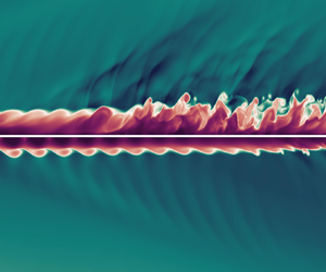
The instantaneous flow structures for the control-off case are visualized in figure 5(a) using Q-isocontours coloured with streamwise vorticity values ( $\omega _x$). The data are extended periodically in the azimuthal direction for illustration purposes. In the upper left-hand corner in figure 5(a), the entire cone, as was used in the experiments, is provided. In the close-up of figure 5(a), the Q-isocontours (Q $= 10^5$) and the contours of the time-averaged Stanton number on the surface of the cone are plotted to indicate the location of the primary streaks relative to the breakdown (generation of small scales). For the control-off case (figure 5a), the Q-isocontours reveal that upstream of the primary streak onset, the flow is dominated by two-dimensional (axisymmetric) structures (due to large amplitude axisymmetric second-mode waves). In the primary streak region, the structures are periodically modulated in the azimuthal direction with the azimuthal wavenumber corresponding to the azimuthal wavenumber of the strongest resonating (fundamental resonance) secondary disturbance wave. In the downstream region where the primary streaks disappear and the secondary streaks begin to form, a ‘quiet’ zone can be observed where the vortical structures are of much lower intensity compared with the primary streak region. The close-up on the bottom of figure 5(a) (using different isocontour levels, $Q = 2\times 10^5$) exposes aligned $\varLambda$-vortices that are typical for a fundamental (or K-type) breakdown. The streamwise vorticity contours show that the ‘legs’ of the $\varLambda$-vortices are counter-rotating. The other close-up in the lower right-hand corner of figure 5(a) displays the hairpin vortices that are generated when the $\varLambda$-vortices begin to break down due to tertiary instabilities (see Klebanoff, Tidstrom & Sargent Reference Klebanoff, Tidstrom and Sargent1962). Towards the end of the computational domain, small-scale structures appear, indicating that the flow has progressed deep into the nonlinear breakdown regime towards turbulent flow. All observations made here for the natural transition scenario without flow control are consistent with the DNS results for a so-called controlled fundamental breakdown (see Hader & Fasel Reference Hader and Fasel2019).

Figure 5. Visualization of the instantaneous flow structures using the Q-criterion coloured by streamwise vorticity  $(\omega_x)$ for control-off (a), and control-on cases with one (b), two (c), and three (d) control strips. $L_{ref}$ is a reference length scale, which in the context of this work is $L_{ref} = 1\ {\rm m}$.
As can be observed for the case with a control strip in figure 5(b), the large amplitude axisymmetric structures appear farther downstream compared with the uncontrolled case. Consequently, all subsequent breakdown stages (e.g. azimuthal modulation, generation of smaller scales) are delayed, thus resulting in a postponed hot streak development and transition. This confirms that the flow control strategy using steady blowing/suction strips remains effective even when transition occurs naturally. This prompts the question if using additional control strips can delay the hot streak development even farther downstream. Towards this end additional control strips, specified in table 1, were applied. As discussed in Hader & Fasel (Reference Hader and Fasel2021a), the most effective location of the control strips is near the primary wave saturation location. Therefore, the additional control strips for the natural transition simulations discussed here were placed based on this rationale. When using two control strips (figure 5c) the hot streaks are shifted all the way to the end of the computational domain and the small-scale generation is no longer observable in the computational domain, thus the late nonlinear stages are not reached in this simulation. With a third control strip (figure 5d), the streaks and the azimuthal modulation no longer appear in the computational domain. Therefore, the control strips successfully delayed transition. Note that there is no requirement for the control strips to have the same width and strength (see table 1) and the control strips could be independently optimized for transition delay.
The time-averaged Stanton number contours on the surface of the cone obtained from the DNS without control strips is provided in figure 6(a) for reference. A description of the streak topology and a comparison with experimental measurements for this case is given in § 3. When using one control strip (figure 6b), the onset of the primary streaks is delayed and the secondary streaks can no longer be observed in the computational domain. The close-up in figure 6(b) also indicates that the control strip slightly alters the hot streak topology. In the control-off case (figure 6a), 80 streaks in the azimuthal direction are obtained (see discussion by Hader & Fasel Reference Hader and Fasel2018) with each streak leading to similar overshoots in the centre of the streak (similar streak ‘strength’ for the selected contour levels). In the control-on case with one control strip, the streak spacing in the azimuthal direction remains the same as in the uncontrolled case; however, every other streak (corresponding to an azimuthal wavenumber of  $k_c=40$) appears to be ‘stronger’ (more prominent for the selected contour levels), indicating that the maximum Stanton number along a streak varies with the azimuthal location. Thus, the control strip seems to affect the dominant azimuthal wavenumber of the secondary disturbance wave.

Figure 6. Time-averaged Stanton number contours on the surface of the cone for the control-off case (a), the control-on cases with one (b), two (c), three (d) control strips.
The primary streaks are delayed even farther downstream when two control strips are employed (see figure 6c), with the same modulation of the hot streak topology as observed for the case with one control strip (figure 6b). An additional third control strip delays the development of the hot streaks so that streaks can no longer be observed in the computational domain (figure 6d).
The development of the time-averaged Stanton number in the downstream direction extracted at an azimuthal location cutting through the centre of a primary streak (with and without control) is shown in figure 7. The control strip locations are again indicated by a dark grey vertical area in figure 7. The Stanton number development obtained from experimental measurements for  $p_0=137.5$ psi, $T_0=408$ K and $Re_1=11.2\times 10^6\, \textrm {m}^{-1}$ digitized from Chynoweth et al. (Reference Chynoweth, Schneider, Hader, Fasel, Batista, Kuehl, Juliano and Wheaton2019) are provided in figure 7(a) for reference. As discussed above, when the control is on, the hot streak formation is substantially delayed (see figure 7a). In addition, the peak Stanton number seems to be slightly reduced when flow control is employed compared with the uncontrolled case. With an additional control strip (figure 7b), the streak development is shifted farther downstream (compounding effect). And with a third control strip (figure 7c), the streak development can no longer be observed in the computational domain.

Figure 7. Time-averaged Stanton number development in the downstream direction extracted at an azimuthal location cutting through a primary streak for the control-off case and the control-on cases with one (a), two (b) and three (c) control strips. The experimental data were digitized from Chynoweth et al. (Reference Chynoweth, Schneider, Hader, Fasel, Batista, Kuehl, Juliano and Wheaton2019) and the control strip locations are highlighted by the dark grey vertical areas.
The amplitude development in the downstream direction of the pressure disturbance at the wall (figure 8) is consulted for understanding how the nonlinear interactions that dominate the laminar–turbulent transition process and hot streak development are affected by the control strips. For the uncontrolled (natural transition) case, the amplitude development was discussed in detail in Hader & Fasel (Reference Hader and Fasel2018). The discussion in this paper is therefore limited to the impact of one and two control strips on select ‘signature’ modes of the fundamental breakdown. As discussed in § 3, the streak development and ultimately laminar–turbulent transition is dominated by a nonlinear interaction of a large amplitude, axisymmetric second-mode (primary) wave and a pair of oblique (secondary) waves at the same frequency. From the numerical investigations by Hader & Fasel (Reference Hader and Fasel2019, Reference Hader and Fasel2018), it is known that, for the investigated geometry and flow conditions, the most amplified axisymmetric second-mode waves are obtained for a frequency of approximately  $f=300$ kHz. In addition, the azimuthal wavenumber, for which the secondary waves experience the strongest fundamental resonance, was found to be $k_c = 80$. Consequently, the nonlinearly generated steady streamwise streaks leading to the hot streak formation also have an azimuthal wavenumber of $k_c = 80$ resulting in 80 streaks around the circumference of the cone, which is in good agreement with the experiments (Chynoweth et al. Reference Chynoweth, Schneider, Hader, Fasel, Batista, Kuehl, Juliano and Wheaton2019). The time-averaged Stanton number contours on the surface of the flared cone (figure 6) demonstrate that while the streak spacing in the azimuthal direction remains unchanged in the control-on case, there is a noticeable variation in the relative strength of the streaks compared with the control-off scenario. Given that every other streak appears fainter, this variation indicates the potential relevance of an azimuthal wavenumber, $k_c=40$. Therefore, the impact of the control strips on these four disturbance wave components (axisymmetric primary and oblique secondary disturbance waves as well as the nonlinearly generated steady streamwise mode, and the steady streamwise mode corresponding to the irregular streak strength) are highlighted in figure 8(a) for one control strip and in figure 8(b) for two control strips. For reference, the amplitude development for the control-off case is provided as black curves in figure 8(a,b). The results clearly show that the control strips disrupt the nonlinear interaction (fundamental resonance) between the axisymmetric primary wave and the oblique secondary waves. This in turn leads to a delay of the development of the steady streamwise modes $(0,80)$ responsible for the hot streak development. After some downstream distance from the control strip, the primary wave resumes its linear growth rate followed by a nonlinear saturation and a strong fundamental resonance, resulting in the streak development and transition to turbulent flow (see figure 8a). For the development of the steady streamwise mode $(0,40)$, as shown at the bottom of figure 8, mode $(0,80)$ is provided as a dashed line for comparison. This illustrates that in the control-off scenario, mode $(0,80)$ exhibits significantly higher amplitudes than mode $(0,40)$, thereby dominating the development of the streamwise streaks and leading to a pattern of regular streak ‘strength.’ Conversely, for the control-on cases, the development of both steady streamwise modes – specifically modes $(0,40)$ and $(0,80)$ – is notably attenuated, resulting in a delayed streak development. However, the control strip impacts each of the steady streamwise modes differently. Mode $(0,40)$ is stabilized to a lesser degree than $(0,80)$. Consequently, both modes attain approximately the same amplitude levels in the downstream region where the hot streaks begin to form on the surface of the cone. The observed variance in streak strength in the control-on cases, as shown in figure 6(b,c), is likely due to the varying degree of stabilization of the steady streamwise modes. As shown in figure 8(b), these interactions can be pushed even farther downstream with multiple control strips. Therefore, the control strategy, using steady blowing/suction strips, as investigated in this paper, can delay the streak development and ultimately transition.

Figure 8. Downstream development of signature modes responsible for the streak development for the control-off (black curves) and the control-on (red curves) cases with one (a), and two (b) control strips. The control strip locations are highlighted by the dark grey vertical areas and the frequency and azimuthal wavenumber of the displayed modes is provided as  $(f,k_c)$ in each of the subplots.
6. Summary
A flow control strategy, using blowing/suction strips at the wall, targeting the nonlinear stages of the natural laminar–turbulent transition process was investigated for a flared cone at Mach 6 for the flow conditions of the Boeing/AFOSR Mach 6 Quiet Tunnel (BAM6QT) and zero angle of attack. For these flow conditions and geometry, the fundamental resonance has been identified to be the relevant nonlinear mechanism. The development of streamwise hot streaks, far exceeding the turbulent values of the Stanton number, was found in the experiments and in DNS. Previously, this flow control method using blowing/suction strips was shown to be effective in delaying the hot streak development for a fundamental resonance initiated with a controlled disturbance input (i.e. initiated by a single frequency disturbance). However, the question is if flow control using steady blowing/suction strips can still effectively prevent transition and the associated detrimental effects when transition occurs naturally. Toward this end, DNS with broadband (random) disturbances introduced at the inflow of the computational domain as a model of natural transition were carried out with and without control strips. The results presented in this paper indicate that this flow control strategy remains effective even when transition is initiated by broadband disturbances. With sufficient blowing/suction strengths, the instantaneous pressure disturbance signals showed a significant shift in the downstream direction of the location where the maximum pressure disturbance amplitudes are observed. The time-averaged Stanton number contours on the surface of the cone confirmed that the control strips can delay the hot streak development and therefore transition. Also, the topology of the hot streaks was altered by the control strips in that the azimuthal wavenumber of the secondary disturbance wave experiencing the strongest secondary instability changes. In both, the uncontrolled and the controlled cases, however, the so-called fundamental resonance was eventually still the dominant nonlinear mechanism leading to the streak development and ultimately transition. Simulations with multiple control strips have shown a compounding effect. For a simulation with three control strips, the hot streaks, and therefore transition, were no longer observable in the computational domain.
Supplementary movie
Supplementary movie is available at https://doi.org/10.1017/jfm.2024.468.
Funding
This work was supported by AFOSR Grant FA9550-19-1-0208, with Dr D. Smith serving as program manager. Computer time was provided by the Department of Defense (DoD) High Performance Computing Modernization Program (HPCMP). The views and conclusions contained herein are those of the authors and should not be interpreted as necessarily representing the official policies or endorsements, either expressed or implied, of the AFOSR or the US Government.
Declaration of interests
The authors report no conflict of interest.


 Open access