


1. Introduction
Formalizing mathematics has a newer and more vivid meaning than it had before. It stands for the task of representing mathematical knowledge in digital form. Formalization in the new sense is close to the implementation of a theory or the verification of knowledge. The basic tools for such a task are the proof assistant programs like Lean, Coq, Agda, and more (Barendregt and Geuvers, Reference Barendregt and Geuvers2001). In order to formalize a piece of mathematics, we should provide equational reasoning and basic definitions of the mentioned theory to our favorite proof assistant, and then we can make formal derivations relying on the previous building blocks. These derivations might be the digitized version of the knowledge that we proved before by hand. In this sense, the task is a kind of verification of the human knowledge done on paper. Moreover, we can see the implementation aspect of the formalization in the proof assistant itself. For example, proof assistants such as Lean, Coq, and Agda implement dependent type theory (Geuvers, Reference Geuvers2009), while Mizar implements Tarski–Grothendieck set theory (Bancerek et al., Reference Bancerek, Byliński, Grabowski, Korniłowicz, Matuszewski, Naumowicz and Pak2018).
As proof assistants become more interactive than before, it is possible to learn more from the formalization process itself. For many mathematicians, using abuse of notation is a natural approach, and it indeed has some benefits. However, when we start to make mathematics precise in a proof assistant, this approach is not allowed. This is one of the significant differences between mathematics on paper and on computer. Therefore, during the formalization task, it is very likely to explore the gaps due to the abuse of formal language. This is an excellent example of what we can learn from proof assistants. From the author’s perspective, it is fair to say that as we teach computers to be clever at mathematics, they teach us to be more clever. This study is an experience of the interaction between a theory discovered by people and its formalization.
The theory subject to the experience is the homotopy type theory (HoTT). It is a new foundational theory for mathematics. It relies on the intuitionistic type theory with a homotopical interpretation. This theory is also known as the Univalent Foundation due to its essential part, the univalence axiom. It roughly says equivalent mathematical objects are equal. HoTT is a relatively new and rapidly evolving field within mathematics. By approaching problems that could be subjects of logic from the perspective of homotopy theory, it offers new perspectives and techniques. It treats higher-categorical structures natively. Also, it is naturally an isomorphism- and equivalence-invariant theory thanks to the univalence. Another essential feature of HoTT is that it is constructed on top of MLTT, which can be practically implemented in proof assistants such as Coq (Bertot and Castéran, Reference Bertot and Castéran2004) and Agda (Norell, Reference Norell2007). However, HoTT lacks modeling of some structures (e.g., semisimplicial types). Thus, there are some efforts to extend HoTT. Two-level type theory (2LTT) is one of these extensions.Footnote 1 Briefly speaking, 2LTT has two levels: a HoTT base level containing only fibrant types and a stricter meta-level whose types – called exo-types – need not be fibrant and which validates the uniqueness of identity proofs. One can think that the second level is the meta-theory of the first. Section 2 aims to analyze the bridge between the two levels in terms of formalized mathematics.
Why do we care about this bridge, although it has already been analyzed on paper? As a reader who is now familiar with proof assistants might guess, the formalization task is not easy compared to the work done on paper. Some definitions need to be changed or adjusted to be applicable to the assistant. Even obvious derivations should be implemented to obtain precise proofs. In other words, there is no room for gaps. In the case of 2LTT, there is no well-accepted formalization for now. Recently, one of the proof assistants, Agda, has released some new features that allow us to work with 2LTT. Moreover, using these, we have developed an Agda library (Uskuplu, Reference Uskuplu2025) about 2LTT and some of its applications. This was one of the first attempts to use these features of Agda. Although the initial goal was to formalize the content of the paper, The Univalence Principle (Ahrens et al., Reference Ahrens, North, Shulman and Tsementzis2025), the basics of 2LTT had to be built first because the study in the mentioned paper is based on 2LTT. Within this experience, some modifications to the definitions and some additional tools were needed. One of our goals is to emphasize these changes and additions that make 2LTT easily applicable in Agda. We provide the details of our library in Section 2.3.
During our Agda project, we encountered situations where certain proofs required the formalization of a new auxiliary tool, which we refer to as function extensionality for cofibrant exo-types (see Proposition 2.12). Functional extensionality is a fundamental property of dependent functions, asserting that two functions are equal if and only if they produce equal results for every input. The specific notion of equality may vary depending on different contexts and levels, but in the case of traditional function extensionality, the equality notion remains consistent both in the domain and the range. However, when dealing with cofibrant exo-types, the situation is different. Here, the equality notions for the input terms and the output terms may differ. Classical funext for fibrant types does not apply here because the domain is not fibrant, while exo-level funext is inapplicable because it speaks only about exo-equality; Proposition 2.12 bridges this gap by relating exo-equality in the domain to ordinary identity in the fibrant codomain. Therefore, in our study, we introduce this novel function extensionality property tailored for such cases, and we rigorously establish its validity. Furthermore, our project led us to uncover novel results related to certain inductive types, notably lists and binary trees, which had not been explored within the context of 2LTT before. What initially started as a foundation for another study has opened up exciting new directions for further research. In Section 4, we also explain why the results about certain types can be an inspiration to a more general case.
One of the original motivations for 2LTT was to define semisimplicial types. However, although plain 2LTT allows defining the type of
 $n$
-truncated semisimplicial types for any exo-natural number
$n$
-truncated semisimplicial types for any exo-natural number
 $n$
, a term of
$n$
, a term of
 $\mathbb{N}$
in the second level, it does not seem possible to assemble these into a type of untruncated semisimplicial types. Voevodsky’s solution (Voevodsky, Reference Voevodsky2013) was to assume that exo-nat,
$\mathbb{N}$
in the second level, it does not seem possible to assemble these into a type of untruncated semisimplicial types. Voevodsky’s solution (Voevodsky, Reference Voevodsky2013) was to assume that exo-nat,
 $\mathbb{N}$
in the second level, is fibrant (isomorphic to a type in the first level), which works for simplicial sets but may not hold in all infinity-toposes. However, assuming cofibrancy, a weaker notion than fibrancy, of exo-nat also allows for defining a fibrant type of untruncated semisimplicial types with a broader syntax, including models for all infinity-toposes. After giving the overview of the models of 2LTT, we provide such models in Section 3.2.
$\mathbb{N}$
in the second level, is fibrant (isomorphic to a type in the first level), which works for simplicial sets but may not hold in all infinity-toposes. However, assuming cofibrancy, a weaker notion than fibrancy, of exo-nat also allows for defining a fibrant type of untruncated semisimplicial types with a broader syntax, including models for all infinity-toposes. After giving the overview of the models of 2LTT, we provide such models in Section 3.2.
Structure of this work
In Section 2, we begin with giving the basics of 2LTT. Our basic objects, types, and exo-types are explained. We then give the three exo-type classifications, which are fibrancy, cofibrancy, and sharpness. Note that these concepts are the basic building blocks of the mentioned study (Ahrens et al., Reference Ahrens, North, Shulman and Tsementzis2025). We also provide new results about the cofibrancy and sharpness of some inductive types. Proposition 2.12 and the entire Section 2.2 are new in this field. Also, we point to the relevant codes in the Agda library and talk about how, if at all, things that differ from previous work contribute to Agda formalization. In Section 3, to present the complete picture, we also explored the semantic aspect of the study and introduced the meaning of 2LTT’s model, providing results about the general models of the theory we were concerned with. As far as we know, there have been no previous studies on non-trivial models of 2LTT with cofibrant exo-nat. By non-trivial, we mean the proposed model satisfies cofibrant exo-nat but does not satisfy fibrant exo-nat.
Relation to the preprint
This article supersedes the arXiv preprint (Uskuplu, Reference Uskuplu2023). The preprint included full, machine-checked proofs of results that also appear in Annenkov et al. (Reference Annenkov, Capriotti, Kraus and Sattler2023) and Ahrens et al. (Reference Ahrens, North, Shulman and Tsementzis2025); because those proofs are now established and reproduced in the public Agda library, we omit them here and provide concise expository summaries with explicit pointers to the library and to the earlier papers. In addition, the many inline Agda side notes scattered through the preprint have been gathered into a single implementation subsection, giving the main text a smoother narrative flow while still directing readers to the exact formalization when needed.
Drawbacks and limitations
Although the proofs in the paper are logically valid and complete, the formalization of 2LTT heavily depends on new, experimental, and undocumented features of Agda. As such, some bugs are emerging from the previously untested interactions of these features, and there might be more than we encountered. There are some efforts by Agda developers to fix these bugs in the Agda source code. We expect the study with these experimental features to produce documentation on what we need to avoid bugs.
2. Two-level type theory - syntax
2.1 Review
We mainly refer to Annenkov et al. (Reference Annenkov, Capriotti, Kraus and Sattler2023) about 2LTT. Basically, we have two different objects in the theory: types in the HoTT level and exo-types in the meta-level. We have similar types of former constructions at both levels. We always make the distinction between types and exo-types using the superscript
 $-^e$
. According to this, the main types we care about are
$-^e$
. According to this, the main types we care about are
 $\prod$
,
$\prod$
,
 $\sum$
,
$\sum$
,
 $+$
,
$+$
,
 $\times$
,
$\times$
,
 $\mathbf{1}$
,
$\mathbf{1}$
,
 $\mathbf{0}$
,
$\mathbf{0}$
,
 $\mathbb{N}$
, and
$\mathbb{N}$
, and
 $\mathbb{N}_{\lt n}$
(finite type of order
$\mathbb{N}_{\lt n}$
(finite type of order
 $n$
),
$n$
),
 $\mathcal{U}$
(universe), and the identity type
$\mathcal{U}$
(universe), and the identity type
 $=$
. Their “exo” versions are denoted by
$=$
. Their “exo” versions are denoted by
 $\prod ^e$
,
$\prod ^e$
,
 $\sum ^e$
,
$\sum ^e$
,
 $+^e$
,
$+^e$
,
 $\times ^e$
,
$\times ^e$
,
 ${\mathbf{1}}^e$
,
${\mathbf{1}}^e$
,
 ${\mathbf{0}}^e$
,
${\mathbf{0}}^e$
,
 $\mathbb{N}^e$
, and
$\mathbb{N}^e$
, and
 $\mathbb{N}^e_{\lt n}$
(exo-finite exo-type of order
$\mathbb{N}^e_{\lt n}$
(exo-finite exo-type of order
 $n$
),
$n$
),
 $\mathcal{U}^e$
(exo-universe), and the exo-equality
$\mathcal{U}^e$
(exo-universe), and the exo-equality
 $\mathsf{=}^{\textit {e}}$
. One can also see Uskuplu (Reference Uskuplu2023) for the detailed definitions. Also, we omit most of the proofs in this section; one can read them in Uskuplu (Reference Uskuplu2023).
$\mathsf{=}^{\textit {e}}$
. One can also see Uskuplu (Reference Uskuplu2023) for the detailed definitions. Also, we omit most of the proofs in this section; one can read them in Uskuplu (Reference Uskuplu2023).
Note that these type/exo-type pairs may not coincide in the cases of
 $+^e$
,
$+^e$
,
 $\mathbb{N}^e$
,
$\mathbb{N}^e$
,
 ${\mathbf{0}}^e$
, and
${\mathbf{0}}^e$
, and
 $\mathsf{=}^{\textit {e}}$
. For example, even if
$\mathsf{=}^{\textit {e}}$
. For example, even if
 $A,B:\mathcal{U}$
, we may not have
$A,B:\mathcal{U}$
, we may not have
 $A +^e B : \mathcal{U}$
; namely, this is always an exo-type but not generally a type. The difference in these cases is that the elimination/induction rules of fibrant types cannot be used unless the target is fibrant. For example, we can define functions into any exo-type by recursion on
$A +^e B : \mathcal{U}$
; namely, this is always an exo-type but not generally a type. The difference in these cases is that the elimination/induction rules of fibrant types cannot be used unless the target is fibrant. For example, we can define functions into any exo-type by recursion on
 $\mathbb{N}^e$
, but if we want to define a function
$\mathbb{N}^e$
, but if we want to define a function
 $f :\mathbb{N} \rightarrow A$
by recursion, we must have
$f :\mathbb{N} \rightarrow A$
by recursion, we must have
 $A : \mathcal{U}$
.
$A : \mathcal{U}$
.
Remark 2.1. We assume the univalence axiom (
 $\mathsf{UA}$
) only for the identity type. Thus, we also have the function extensionality (
$\mathsf{UA}$
) only for the identity type. Thus, we also have the function extensionality (
 $\mathsf{funext}$
) for it. For the exo-equality, we assume the
$\mathsf{funext}$
) for it. For the exo-equality, we assume the
 $\mathsf{funext}$
and the axiom called uniqueness of identity proofs (
$\mathsf{funext}$
and the axiom called uniqueness of identity proofs (
 $\mathsf{UIP}$
). In other words, we have the following
$\mathsf{UIP}$
). In other words, we have the following
-
•
 $\mathsf{UA} : \prod _{A,B : \mathcal{U}} (A \simeq B) \rightarrow (A = B)$
-
•
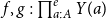
${\mathsf{funext}} : \left (f,g : \prod _A B(a) \right ) \rightarrow \left ( \prod _{a : A} f(a)=g(a) \rightarrow (f=g) \right )$
-
•
${\mathsf{funext}}^e : \left (f,g : \prod ^e_A B(a) \right ) \rightarrow \left ( \prod ^e_{a : A} f(a){\mathsf{=}^{\textit {e}}} g(a) \rightarrow (f{\mathsf{=}^{\textit {e}}} g) \right )$
-
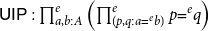
•
${\mathsf{UIP}} : \prod ^e_{a,b :A} \left ( \prod ^e_{(p,q : a{\mathsf{=}^{\textit {e}}} b)} p {\mathsf{=}^{\textit {e}}} q \right )$


In the applications or examples, we often make use of both versions of
 $\mathsf{funext}$
.
$\mathsf{funext}$
.
Remark 2.2. Just as there is a type hierarchy regarding path types such as contractible types, propositions, and sets, we can define exo-contractible exo-type, exo-propositions, and exo-sets similarly concerning
 $\mathsf{=}^{\textit {e}}$
. Since we assume
$\mathsf{=}^{\textit {e}}$
. Since we assume
 $\mathsf{UIP}$
for exo-equality, this yields that all exo-types are exo-sets. On another note, any property of
$\mathsf{UIP}$
for exo-equality, this yields that all exo-types are exo-sets. On another note, any property of
 $=$
can be defined for
$=$
can be defined for
 $\mathsf{=}^{\textit {e}}$
similarly by its elimination rule. For example, we have both transport (
$\mathsf{=}^{\textit {e}}$
similarly by its elimination rule. For example, we have both transport (
 $\mathsf{tr}$
) and exo-transport (
$\mathsf{tr}$
) and exo-transport (
 $\mathsf{tr}^e$
), and we have both path-type homotopies (
$\mathsf{tr}^e$
), and we have both path-type homotopies (
 $\sim$
) of functions between types and exo-equality homotopies (
$\sim$
) of functions between types and exo-equality homotopies (
 $\sim ^e$
) of functions between exo-types, and so on. We refer to the HoTT Book (HoTTBook, 2013) for these kinds of properties not defined here.
$\sim ^e$
) of functions between exo-types, and so on. We refer to the HoTT Book (HoTTBook, 2013) for these kinds of properties not defined here.
Considering these twin definitions, it’s natural to ask whether there is a correspondence between them. We obtain such a correspondence according to the relation between types and exo-types. Annenkov et al. (Reference Annenkov, Capriotti, Kraus and Sattler2023), it is assumed that there is a coercion map
 $c$
from types to exo-types; for any type
$c$
from types to exo-types; for any type
 $A : \mathcal{U}$
, we have
$A : \mathcal{U}$
, we have
 $c(A) : \mathcal{U}^e$
. Another approach, as in Ahrens et al. (Reference Ahrens, North, Shulman and Tsementzis2025), is taking
$c(A) : \mathcal{U}^e$
. Another approach, as in Ahrens et al. (Reference Ahrens, North, Shulman and Tsementzis2025), is taking
 $c$
as an inclusion; in other words, assuming every type is an exo-type. In this work, the second approach is assumed. Therefore, we can apply exo-type formers to types. For example, both
$c$
as an inclusion; in other words, assuming every type is an exo-type. In this work, the second approach is assumed. Therefore, we can apply exo-type formers to types. For example, both
 $\mathbb{N} + \mathbb{N}$
and
$\mathbb{N} + \mathbb{N}$
and
 $\mathbb{N} +^e \mathbb{N}$
make sense, but both are still exo-types. We will later prove some isomorphisms related to such correspondences.
$\mathbb{N} +^e \mathbb{N}$
make sense, but both are still exo-types. We will later prove some isomorphisms related to such correspondences.
We define the exo-type of exo-isomorphisms between
 $A,B : \mathcal{U}^e$
(or briefly isomorphisms) as
$A,B : \mathcal{U}^e$
(or briefly isomorphisms) as
 \begin{equation*}A \cong B \;:=\; {\sum }^e_{f:A\rightarrow B}{\sum }^e_{g:B\rightarrow A}(f {{\circ }^{\textit {e}}} g {\mathsf{=}^{\textit {e}}} \mathsf{id}_B) \times ^e(g {{\circ }^{\textit {e}}} f {\mathsf{=}^{\textit {e}}} \mathsf{id}_A).\end{equation*}
We define the type of equivalences between
 $A,B : \mathcal{U}$
as
$A,B : \mathcal{U}$
as
 \begin{equation*}A \simeq B \;:=\; \sum _{f:A\rightarrow B} \left ( \prod _{b:B} \texttt {is-Contr}\left (\sum _{a:A} f(a)=b\right )\right ).\end{equation*}
Also,
 $f$
function
$f$
function
 $f : A \rightarrow B$
between types is called quasi-invertible if there is a function
$f : A \rightarrow B$
between types is called quasi-invertible if there is a function
 $g : B \rightarrow A$
such that
$g : B \rightarrow A$
such that
 $g \circ f = \mathsf{id}_A$
and
$g \circ f = \mathsf{id}_A$
and
 $f \circ g = \mathsf{id}_B$
where
$f \circ g = \mathsf{id}_B$
where
 $\mathsf{id}_A : A \rightarrow A$
is the identity map.
$\mathsf{id}_A : A \rightarrow A$
is the identity map.
Remark 2.3. In these definitions, one can use
 ${\mathsf{funext}}^e$
or
${\mathsf{funext}}^e$
or
 $\mathsf{funext}$
, and instead of showing, for example,
$\mathsf{funext}$
, and instead of showing, for example,
 $g {{\circ }^{\textit {e}}} f {\mathsf{=}^{\textit {e}}} \mathsf{id}_A$
, it can be shown that
$g {{\circ }^{\textit {e}}} f {\mathsf{=}^{\textit {e}}} \mathsf{id}_A$
, it can be shown that
 $g (f (a)) = a$
for any
$g (f (a)) = a$
for any
 $a \in A$
. Moreover, a map is an equivalence if and only if it is quasi-invertible. Therefore, we can use both interchangeably. For practical purposes, when we need to show that
$a \in A$
. Moreover, a map is an equivalence if and only if it is quasi-invertible. Therefore, we can use both interchangeably. For practical purposes, when we need to show that
 $f$
is an equivalence, we generally do it by showing that it is quasi-invertible.
$f$
is an equivalence, we generally do it by showing that it is quasi-invertible.
Assuming that each type is an exo-type and considering all definitions so far, the correspondence between exo-type formers and type formers can be characterizedFootnote 2 as follows.
Theorem 2.4.
If
 $A, C: \mathcal{U}$
are types and
$A, C: \mathcal{U}$
are types and
 $B : A \rightarrow \mathcal{U}$
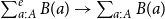
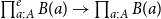
is a type family, we have the following maps. The first three maps are exo-isomorphisms.
$B : A \rightarrow \mathcal{U}$
is a type family, we have the following maps. The first three maps are exo-isomorphisms.
-
i.
${\mathbf{1}}^e \rightarrow {\mathbf{1}}$
, -
ii.
$\sum ^e_{a:A} B(a) \rightarrow \sum _{a:A} B(a)$
, -
iii.
$\prod ^e_{a:A} B(a) \rightarrow \prod _{a:A} B(a)$
, -
iv.
$A +^e C \rightarrow A + C$
, -
v.
${\mathbf{0}}^e \rightarrow {\mathbf{0}}$
, -
vi.
$\mathbb{N}^e \rightarrow \mathbb{N}$
, -
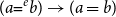
vii. For any
$a,b:A$
, we have
$(a{\mathsf{=}^{\textit {e}}} b) \rightarrow (a = b)$
.


Remark 2.5. It is worth emphasizing that the inverses of the maps iv, v, and vi can be assumed to exist. There are some models where these hold (for the details, see the discussion below Lemma 2.11 (Annenkov et al., Reference Annenkov, Capriotti, Kraus and Sattler2023)). However, a possible inverse for the map vii would yield a contradiction because the univalence axiom is inconsistent with the uniqueness of identity proofs. This conversion from the exo-equality (
 $\mathsf{=}^{\textit {e}}$
) to the identity (
$\mathsf{=}^{\textit {e}}$
) to the identity (
 $=$
) still has an importance in many proofs later. Thus we denote it by
$=$
) still has an importance in many proofs later. Thus we denote it by
 \begin{equation*}{\mathsf{eqtoid}} : {\prod _{a,b:A}}^e(a{\mathsf{=}^{\textit {e}}} b) \rightarrow (a = b) \,.\end{equation*}
One of its valuable corollaries is the following lemma.
Lemma 2.6.
Let
 $A,B : \mathcal{U}$
be two types. If
$A,B : \mathcal{U}$
be two types. If
 $A\cong B$
, then
$A\cong B$
, then
 $A\simeq B$
.
$A\simeq B$
.
In terms of the relationship between types and exo-types, there are three classes of exo-types. The first one pertains to the notion of fibrant exo-types.
Definition 2.7.
An exo-type
 $A : \mathcal{U}^e$
is called a
fibrant exo-type
if there is a type
$A : \mathcal{U}^e$
is called a
fibrant exo-type
if there is a type
 $RA : \mathcal{U}$
such that
$RA : \mathcal{U}$
such that
 $A$
and
$A$
and
 $RA$
are exo-isomorphic. In other words,
$RA$
are exo-isomorphic. In other words,
 $A$
is fibrant when the following exo-type is inhabited
$A$
is fibrant when the following exo-type is inhabited
 \begin{equation*}{\mathsf{isFibrant}}(A)\;:=\;{\sum _{RA : \mathcal{U}}}^e (A \cong RA)\,.\end{equation*}
Proposition 2.8 (Annenkov et al., Reference Annenkov, Capriotti, Kraus and Sattler2023). The following are true:
-
i. Any type
$A : \mathcal{U}$
is a fibrant exo-type.
-
ii. The unit exo-type
${\mathbf{1}}^e$
is fibrant.
-
iii. Let
$A : \mathcal{U}^e$
and
$B : A \rightarrow \mathcal{U}^e$
, if
$A$
is fibrant, and each
$B(a)$
is fibrant, then both
$\sum ^e_{a:A} B(a)$
and
$\prod ^e_{a:A} B(a)$
are fibrant.
-
iv. If
$A,B : \mathcal{U}^e$
are exo-isomorphic types, then
$A$
is fibrant if and only if
$B$
is fibrant.
-
v. If
$A:\mathcal{U}^e$
is fibrant, and there are two types
$B,C :\mathcal{U}$
such that
$A\cong B$
and
$A\cong C$
, then
$B=C$
.


Definition 2.9.
Let
 $A,B: \mathcal{U}^e$
be two fibrant exo-types,and
$A,B: \mathcal{U}^e$
be two fibrant exo-types,and
 $f:A\rightarrow B$
. Let
$f:A\rightarrow B$
. Let
 $RA,RB:\mathcal{U}$
be such that
$RA,RB:\mathcal{U}$
be such that
 $A\cong RA$
and
$A\cong RA$
and
 $B\cong RB$
. We have the following diagram.
$B\cong RB$
. We have the following diagram.

We call
 $f$
a
fibrant-equivalence
if
$f$
a
fibrant-equivalence
if
 \begin{equation*}r_B{{\circ }^{\textit {e}}} f {{\circ }^{\textit {e}}} s_A : RA \rightarrow RB\end{equation*}
is an equivalence.
Proposition 2.10.
Let
 $A,B,C: \mathcal{U}^e$
be fibrant exo-types and
$A,B,C: \mathcal{U}^e$
be fibrant exo-types and
 $f:A\rightarrow B$
and
$f:A\rightarrow B$
and
 $g:B \rightarrow C$
. Consider the corresponding diagram.
$g:B \rightarrow C$
. Consider the corresponding diagram.

The following are true:
-
i. If
$f$
is an exo-isomorphism, then it is a fibrant-equivalence.
-
ii. If
$f,g$
are fibrant-equivalences, then so is
$g{{\circ }^{\textit {e}}} f$
. -
iii. If
$f,f'$
are homotopic with respect to
$\mathsf{=}^{\textit {e}}$
, and
$f$
is a fibrant-equivalence, then
$f'$
is a fibrant-equivalence, too.


The second class of exo-types is the cofibrant exo-types.
Definition 2.11 (Corollary 3.19(i) in Annenkov et al. (Reference Annenkov, Capriotti, Kraus and Sattler2023)). Let
 $A:\mathcal{U}^e$
be an exo-type. We call it
cofibrant
if (1) for any type family
$A:\mathcal{U}^e$
be an exo-type. We call it
cofibrant
if (1) for any type family
 $Y : A \rightarrow \mathcal{U}$
over
$Y : A \rightarrow \mathcal{U}$
over
 $A$
, the exo-type
$A$
, the exo-type
 $\prod ^e_{a:A} Y(a)$
is fibrant, and (2) in this case, if
$\prod ^e_{a:A} Y(a)$
is fibrant, and (2) in this case, if
 $Y(a)$
is contractible for each
$Y(a)$
is contractible for each
 $a:A$
, then so is the fibrant match of
$a:A$
, then so is the fibrant match of
 $\prod ^e_{a:A} Y(a)$
.
$\prod ^e_{a:A} Y(a)$
.
The following gives a logically equivalent definition of cofibrancy, which is a novel result. Attention should be paid to the use of
 $=$
and
$=$
and
 $\mathsf{=}^{\textit {e}}$
in order to indicate whether the terms belong to the type or the exo-type.
$\mathsf{=}^{\textit {e}}$
in order to indicate whether the terms belong to the type or the exo-type.
Proposition 2.12.
Let
 $A:\mathcal{U}^e$
be an exo-type such that for any type family
$A:\mathcal{U}^e$
be an exo-type such that for any type family
 $Y : A \rightarrow \mathcal{U}$
over
$Y : A \rightarrow \mathcal{U}$
over
 $A$
, the exo-type
$A$
, the exo-type
 $\prod ^e_{a:A} Y(a)$
is fibrant. Then, the following are equivalent.
$\prod ^e_{a:A} Y(a)$
is fibrant. Then, the following are equivalent.
-
i. In the case above, if
$Y(a)$
is contractible for each
$a:A$
, then so is its fibrant match of
$\prod ^e_{a:A} Y(a)$
; namely,
$A$
is cofibrant.
-
ii. (Function extensionality for cofibrant exo-types). In the case above, for any
$f,g : \prod ^e_{a:A} Y(a)$
if
$f(a)=g(a)$
for each
$a:A$
, then
$r(f)=r(g)$
where
$FM : \mathcal{U}$
and


Proof.
(i
 $\Rightarrow$
ii) Let
$\Rightarrow$
ii) Let
 $f,g : \prod ^e_{a:A} Y(a)$
be such that
$f,g : \prod ^e_{a:A} Y(a)$
be such that
 $t_a : f(a)=g(a)$
for each
$t_a : f(a)=g(a)$
for each
 $a:A$
. Consider another type family
$a:A$
. Consider another type family
 $Y' : A \rightarrow \mathcal{U}$
defined as
$Y' : A \rightarrow \mathcal{U}$
defined as
 \begin{equation*}Y'(a)\;:=\;\sum _{b:B(a)} b=f(a).\end{equation*}
Then both
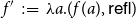 $f'\;:=\;\lambda a.(f(a),{\mathsf{refl}})$
and
$f'\;:=\;\lambda a.(f(a),{\mathsf{refl}})$
and
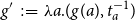 $g'\;:=\;\lambda a. (g(a),t_a^{-1})$
are terms in
$g'\;:=\;\lambda a. (g(a),t_a^{-1})$
are terms in
 $\prod ^e_{a:A}Y'(a)$
. By our assumptions, there is a
$\prod ^e_{a:A}Y'(a)$
. By our assumptions, there is a
 $FM':\mathcal{U}$
such that
$FM':\mathcal{U}$
such that

Since the type of paths at a point is contractible, we have each
 $Y'(a)$
is contractible. By the assumption (i), we get
$Y'(a)$
is contractible. By the assumption (i), we get
 $FM'$
is contractible, and hence
$FM'$
is contractible, and hence
 \begin{equation} r'(f)=r'(g). \end{equation}
Using this, we have the following chain of identities:
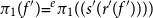
 \begin{equation*} r(f)=r(\pi _1(s'(r'(f'))))=r(\pi _1(s'(r'(g'))))=r(g). \end{equation*}
The first (and the third, by symmetry) identity is obtained as follows: Because
 $r'$
and
$r'$
and
 $s'$
are exo-inverses of each other, we have
$s'$
are exo-inverses of each other, we have
 \begin{equation*}(a:A)\rightarrow \pi _1(f'(a)){\mathsf{=}^{\textit {e}}} \pi _1 ((s'(r'(f'))) (a)).\end{equation*}
Thus, by
 ${\mathsf{funext}}^e$
, we get
${\mathsf{funext}}^e$
, we get
 $\pi _1(f'){\mathsf{=}^{\textit {e}}} \pi _1 ((s'(r'(f'))))$
. Then we applyFootnote
3
$\pi _1(f'){\mathsf{=}^{\textit {e}}} \pi _1 ((s'(r'(f'))))$
. Then we applyFootnote
3
 $r$
to the equality and make it an identity via
$r$
to the equality and make it an identity via
 $\mathsf{eqtoid}$
because the terms are in
$\mathsf{eqtoid}$
because the terms are in
 $FM'$
which is a type.
$FM'$
which is a type.
The second identity is obtained by applying the function
 \begin{equation*}\lambda x. r (\lambda a. \pi _1((s' x) (a))) : FM' \rightarrow FM\end{equation*}
to the identity 1, so we are done.
Note that even if
 $r$
has an exo-type domain and
$r$
has an exo-type domain and
 $s'$
has an exo-type codomain, we can compose these in a way that the resulting map is from a type to a type. Thus, we can apply it to an identity.
$s'$
has an exo-type codomain, we can compose these in a way that the resulting map is from a type to a type. Thus, we can apply it to an identity.
(ii
 $\Rightarrow$
i) Suppose
$\Rightarrow$
i) Suppose
 $Y(a)$
is contractible for each
$Y(a)$
is contractible for each
 $a:A$
. We want to show that
$a:A$
. We want to show that
 $FM$
is contractible where
$FM$
is contractible where

Let
 $b_a :Y(a)$
be the center of contraction for each
$b_a :Y(a)$
be the center of contraction for each
 $a:A$
. Then this gives a function
$a:A$
. Then this gives a function
 $f\;:=\;\lambda a. b_a :\prod ^e_{a:A} Y(a)$
. For any
$f\;:=\;\lambda a. b_a :\prod ^e_{a:A} Y(a)$
. For any
 $x:FM$
, since
$x:FM$
, since
 $f(a)=b_a=s(x)(a)$
for each
$f(a)=b_a=s(x)(a)$
for each
 $a:A$
by contractibility, using the assumption (ii), we get
$a:A$
by contractibility, using the assumption (ii), we get
 $r(f)=r(s(x))$
. Applying
$r(f)=r(s(x))$
. Applying
 $\mathsf{eqtoid}$
to the exo-equality
$\mathsf{eqtoid}$
to the exo-equality
 $r(s(x)){\mathsf{=}^{\textit {e}}} x$
, we get
$r(s(x)){\mathsf{=}^{\textit {e}}} x$
, we get
 $r(f)=x$
. Therefore,
$r(f)=x$
. Therefore,
 $FM$
is contractible with the center of contraction
$FM$
is contractible with the center of contraction
 $r(f)$
.
$r(f)$
.
Cofibrant exo-types have the following properties.
Proposition 2.13 (Annenkov et al., Reference Annenkov, Capriotti, Kraus and Sattler2023).
-
i. All fibrant exo-types are cofibrant.
-
ii. If
$A$
and
$B$
are exo-types such that
$A\cong B$
, and if
$A$
is cofibrant, then
$B$
is cofibrant.
-
iii.
${\mathbf{0}}^e$
is cofibrant, and if
$A,B:\mathcal{U}^e$
are cofibrant, then so are
$A+^eB$
and
$A\times ^eB$
. In particular, all exo-finite exo-types are cofibrant.
-
iv. If
$A:\mathcal{U}^e$
is cofibrant and
$B:A\rightarrow \mathcal{U}^e$
is such that each
$B(a)$
is cofibrant, then
$\sum ^e_{a:A} B(a)$
is cofibrant.


Another class of exo-types is the class of sharp ones. This was given in Ahrens et al. (Reference Ahrens, North, Shulman and Tsementzis2025) for the first time.
Definition 2.14 (Definition 2.2 in Ahrens et al. (Reference Ahrens, North, Shulman and Tsementzis2025)). An exo-type
 $A$
is
sharp
if it is cofibrant and it has a “fibrant replacement”, meaning that there is a fibrant type
$A$
is
sharp
if it is cofibrant and it has a “fibrant replacement”, meaning that there is a fibrant type
 $RA$
and a map
$RA$
and a map
 $r : A \rightarrow RA$
such that for any family of types
$r : A \rightarrow RA$
such that for any family of types
 $Y : RA \rightarrow \mathcal{U}$
, the precomposition map below is a fibrant-equivalence (recall Definition 2.9).
$Y : RA \rightarrow \mathcal{U}$
, the precomposition map below is a fibrant-equivalence (recall Definition 2.9).
 \begin{equation} (\!- {{\circ }^{\textit {e}}} r):\prod _{c:RA} Y(c) \rightarrow {\prod _{a:A}}^e Y(r(a)) \end{equation}
The following lemma gives another definition for sharp exo-types. First, we need an auxiliary definition.
Definition 2.15.
Let
 $A,B: \mathcal{U}^e$
be two fibrant exo-types and
$A,B: \mathcal{U}^e$
be two fibrant exo-types and
 $f:A\rightarrow B$
be a map. Let
$f:A\rightarrow B$
be a map. Let
 $RA,RB:\mathcal{U}$
be such that
$RA,RB:\mathcal{U}$
be such that
 $A\cong RA$
and
$A\cong RA$
and
 $B\cong RB$
. Take
$B\cong RB$
. Take
 $s_A:RA \rightarrow A$
and
$s_A:RA \rightarrow A$
and
 $r_B:B \rightarrow RB$
as these isomorphisms. Then
$r_B:B \rightarrow RB$
as these isomorphisms. Then
 $f$
has a
fibrant-section
if
$f$
has a
fibrant-section
if
 \begin{equation*}r_B{{\circ }^{\textit {e}}} f {{\circ }^{\textit {e}}} s_A : RA \rightarrow RB\end{equation*}
has a section.
Lemma 2.16 (Ahrens et al., Reference Ahrens, North, Shulman and Tsementzis2025). Let
 $A$
be a cofibrant exo-type,
$A$
be a cofibrant exo-type,
 $RA$
a type, and
$RA$
a type, and
 $r:A \rightarrow RA$
a map. The following are equivalent:
$r:A \rightarrow RA$
a map. The following are equivalent:
-
(1) The map ( 2 ) is a fibrant-equivalence for any
$Y:RA\rightarrow \mathcal{U}$
, so that
$A$
is sharp.
-
(2) The map ( 2 ) has a fibrant-section for any
$Y:RA\rightarrow \mathcal{U}$
. -
(3) The map ( 2 ) is a fibrant-equivalence whenever
$Y\;:=\;\lambda x. Z$
for a constant type
$Z:\mathcal{U}$
, hence
$RA \rightarrow Z$
is equivalent to the fibrant match of
$A \rightarrow Z$
.


As in the cofibrant exo-types, the notion of sharpness has its own preservation rules. The following proposition gives these rules.
Proposition 2.17 (Ahrens et al., Reference Ahrens, North, Shulman and Tsementzis2025). The following are true.
-
i. All fibrant exo-types are sharp.
-
ii. If
$A$
and
$B$
are exo-types such that
$A\cong B$
, and if
$A$
is sharp, then
$B$
is sharp.
-
iii.
${\mathbf{0}}^e$
is sharp, and if
$A$
and
$B$
are sharp exo-types, then so are
$A +^e B$
and
$A \times ^e B$
. -
iv. If
$A$
is a sharp exo-type,
$B : A \rightarrow \mathcal{U}$
is such that each
$B(a)$
is sharp, then
$\sum ^e_{a:A} B(a)$
is sharp.
-
v. Each finite exo-type
$\mathbb{N}^e_{\lt n}$
is sharp.
-
vi. If
$\mathbb{N}^e$
is cofibrant, then it is sharp.


2.2 Lifting cofibrancy from exo-nat to other types
In this section, we give a new result about other inductive types. After this paper was written, the referee helpfully observed that the two examples treated below (List and BinaryTree) can be expressed as
 $F(A)$
where
$F(A)$
where
 $A$
is (sharp) cofibrant and
$A$
is (sharp) cofibrant and
 $F$
is a container, equivalently, a polynomial functor whose shape exo-type is countable and each position fiber is finite (Abbott et al., Reference Abbott, Altenkirch and Ghani2005; Gambino and Kock, Reference Gambino and Kock2013). Although our original proofs establish (sharpness) cofibrancy directly and were found independently of the container formalism, this perspective is indeed worth recording: the closureFootnote
4
of (sharp) cofibrant exo-types under countable coproducts and finite products implies that any such container application preserves cofibrancy. The results below are therefore special cases of this more general closure principle.
$F$
is a container, equivalently, a polynomial functor whose shape exo-type is countable and each position fiber is finite (Abbott et al., Reference Abbott, Altenkirch and Ghani2005; Gambino and Kock, Reference Gambino and Kock2013). Although our original proofs establish (sharpness) cofibrancy directly and were found independently of the container formalism, this perspective is indeed worth recording: the closureFootnote
4
of (sharp) cofibrant exo-types under countable coproducts and finite products implies that any such container application preserves cofibrancy. The results below are therefore special cases of this more general closure principle.
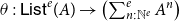
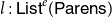
2.2.1 List (exo)types
Definition 2.18.
For an exo-type
 $A:\mathcal{U}^e$
, we define the exo-type
$A:\mathcal{U}^e$
, we define the exo-type
 ${\mathsf{List}}^e (A) : \mathcal{U}^e$
of
finite exo-lists
of terms of
${\mathsf{List}}^e (A) : \mathcal{U}^e$
of
finite exo-lists
of terms of
 $A$
, which has constructors
$A$
, which has constructors
-
•
${\mathsf{[]}}^e : {\mathsf{List}}^e (A)$
-
•
$\mathsf{::}^e : A \rightarrow {\mathsf{List}}^e (A) \rightarrow {\mathsf{List}}^e (A)$


Similarly, if
 $A : \mathcal{U}$
is a type, the type
$A : \mathcal{U}$
is a type, the type
 ${\mathsf{List}}(A)$
of
finite lists
of
${\mathsf{List}}(A)$
of
finite lists
of
 $A$
has constructors
$A$
has constructors
 $\mathsf{[]}$
and
$\mathsf{[]}$
and
 $\mathsf{::}\,$
.
$\mathsf{::}\,$
.
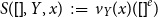
As in Theorem2.4, we have an obvious map
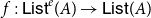 $f : {\mathsf{List}}^e (A) \rightarrow {\mathsf{List}} (A)$
for a type
$f : {\mathsf{List}}^e (A) \rightarrow {\mathsf{List}} (A)$
for a type
 $A$
defined as
$A$
defined as
 $f({\mathsf{[]}}^e)\;:=\;{\mathsf{[]}}$
and
$f({\mathsf{[]}}^e)\;:=\;{\mathsf{[]}}$
and
 $f(a\,\mathsf{::}^e\, l)\;:=\;a\, \mathsf{::}\, f(l)$
. We will give some conditions for cofibrancy and sharpness of
$f(a\,\mathsf{::}^e\, l)\;:=\;a\, \mathsf{::}\, f(l)$
. We will give some conditions for cofibrancy and sharpness of
 ${\mathsf{List}}^e (A)$
. Indeed, if we assume
${\mathsf{List}}^e (A)$
. Indeed, if we assume
 $\mathbb{N}^e$
and
$\mathbb{N}^e$
and
 $A$
are cofibrant, then we can show
$A$
are cofibrant, then we can show
 ${\mathsf{List}}^e (A)$
is cofibrant. The proof is obtained by an isomorphism between a cofibrant exo-type and
${\mathsf{List}}^e (A)$
is cofibrant. The proof is obtained by an isomorphism between a cofibrant exo-type and
 ${\mathsf{List}}^e(A)$
. The same isomorphism shows that
${\mathsf{List}}^e(A)$
. The same isomorphism shows that
 ${\mathsf{List}}^e (A)$
is sharp if
${\mathsf{List}}^e (A)$
is sharp if
 $A$
is also sharp. Moreover, we can show the sharpness of
$A$
is also sharp. Moreover, we can show the sharpness of
 ${\mathsf{List}}^e(A)$
in a way analogous to Proposition 2.17(vi).
${\mathsf{List}}^e(A)$
in a way analogous to Proposition 2.17(vi).
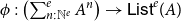
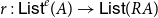
Lemma 2.19.
Let
 $A : \mathcal{U}^e$
be an exo-type. Then we have
$A : \mathcal{U}^e$
be an exo-type. Then we have
 \begin{equation*}\left ( {\sum _{n:\mathbb{N}^e}}^e A^n \right ) \cong {\mathsf{List}}^e(A)\end{equation*}
where
 $A^{{\mathsf{0}}^e}\;:=\;{\mathbf{1}}^e$
and
$A^{{\mathsf{0}}^e}\;:=\;{\mathbf{1}}^e$
and
 $A^{({\mathsf{succ}}^e n)} \;:=\; A \times ^e A^n$
.
$A^{({\mathsf{succ}}^e n)} \;:=\; A \times ^e A^n$
.
Proof.
Define
 $\phi : \left (\sum ^e_{n:\mathbb{N}^e} A^n\right ) \rightarrow {\mathsf{List}}^e(A)$
as follows
$\phi : \left (\sum ^e_{n:\mathbb{N}^e} A^n\right ) \rightarrow {\mathsf{List}}^e(A)$
as follows
 \begin{eqnarray*} \phi ({\mathsf{0}}^e, \star ^e)&\;:=\;& {\mathsf{[]}}^e\\ \phi ({\mathsf{succ}}^e(n), (a,p))&\;:=\;& a\, \mathsf{::}^e\, \phi (n,p). \end{eqnarray*}
Define
 $\theta : {\mathsf{List}}^e(A) \rightarrow \left (\sum ^e_{n:\mathbb{N}^e} A^n\right )$
as follows,
$\theta : {\mathsf{List}}^e(A) \rightarrow \left (\sum ^e_{n:\mathbb{N}^e} A^n\right )$
as follows,
 \begin{eqnarray*} \theta ({\mathsf{[]}}^e)&\;:=\;& ({\mathsf{0}}^e, \star ^e)\\ \theta (a \,\mathsf{::}^e\, l)&\;:=\;&({\mathsf{succ}}^e(\pi ^e_1\,\theta (l))\,,(a,\pi ^e_2\,\theta (l))). \end{eqnarray*}
Then, it is easy to show by the induction on the constructors that
 \begin{equation*}\phi {{\circ }^{\textit {e}}} \theta {\mathsf{=}^{\textit {e}}} \mathsf{id}_{{\mathsf{List}}^e(A)}\quad \text{and}\quad \theta {{\circ }^{\textit {e}}} \phi {\mathsf{=}^{\textit {e}}} \mathsf{id}_{\sum ^e_{n:\mathbb{N}^e} A^n}.\end{equation*}
Proposition 2.20.
If
 $A:\mathcal{U}^e$
is cofibrant and
$A:\mathcal{U}^e$
is cofibrant and
 $\mathbb{N}^e$
is cofibrant, then so is
$\mathbb{N}^e$
is cofibrant, then so is
 ${\mathsf{List}}^e(A)$
.
${\mathsf{List}}^e(A)$
.
Proof.
By Lemma 2.19 and Proposition 2.13(ii), it is enough to show that
 $\sum ^e_{n:\mathbb{N}^e} A^n$
is cofibrant. By the assumption and 2.13(iii), we have
$\sum ^e_{n:\mathbb{N}^e} A^n$
is cofibrant. By the assumption and 2.13(iii), we have
 $A^n$
is a cofibrant exo-type for all
$A^n$
is a cofibrant exo-type for all
 $n:\mathbb{N}^e$
. Since we also assume
$n:\mathbb{N}^e$
. Since we also assume
 $\mathbb{N}^e$
is cofibrant, we are done by 2.13(iv).
$\mathbb{N}^e$
is cofibrant, we are done by 2.13(iv).
By similar reasoning, we obtain that
 ${\mathsf{List}}^e(A)$
is sharp if
${\mathsf{List}}^e(A)$
is sharp if
 $A$
is sharp and
$A$
is sharp and
 $\mathbb{N}^e$
is cofibrant. However, we can also show the sharpness of
$\mathbb{N}^e$
is cofibrant. However, we can also show the sharpness of
 ${\mathsf{List}}^e(A)$
, like in Proposition 2.17(vi).
${\mathsf{List}}^e(A)$
, like in Proposition 2.17(vi).
Proposition 2.21.
Let
 $A:\mathcal{U}^e$
be a sharp exo-type. Suppose also that
$A:\mathcal{U}^e$
be a sharp exo-type. Suppose also that
 $\mathbb{N}^e$
is cofibrant. Then
$\mathbb{N}^e$
is cofibrant. Then
 ${\mathsf{List}}^e(A)$
is sharp.
${\mathsf{List}}^e(A)$
is sharp.
Proof.
Since
 $A$
is sharp, it is cofibrant. By Proposition 2.20, we have
$A$
is sharp, it is cofibrant. By Proposition 2.20, we have
 ${\mathsf{List}}^e(A)$
is cofibrant, so it remains to find the fibrant replacement of it.
${\mathsf{List}}^e(A)$
is cofibrant, so it remains to find the fibrant replacement of it.
Since
 $A$
is sharp, we have a type
$A$
is sharp, we have a type
 $RA:\mathcal{U}$
and a map
$RA:\mathcal{U}$
and a map
 $r_A:A\rightarrow RA$
such that the map 2 is a fibrant-equivalence for any
$r_A:A\rightarrow RA$
such that the map 2 is a fibrant-equivalence for any
 $Y:RA \rightarrow \mathcal{U}$
. We claim that
$Y:RA \rightarrow \mathcal{U}$
. We claim that
 ${\mathsf{List}} (RA)$
is a fibrant replacement of
${\mathsf{List}} (RA)$
is a fibrant replacement of
 ${\mathsf{List}}^e(A)$
. Define
${\mathsf{List}}^e(A)$
. Define
 $r:{\mathsf{List}}^e(A)\rightarrow {\mathsf{List}} (RA)$
as
$r:{\mathsf{List}}^e(A)\rightarrow {\mathsf{List}} (RA)$
as
 \begin{eqnarray*} r({\mathsf{[]}}^e)&\;:=\;&{\mathsf{[]}}\\ r(a\, \mathsf{::}^e\, l)&\;:=\;&r_A(a) \,\mathsf{::}\, r(l) \end{eqnarray*}
Consider the following commutative diagram for any
 $Y: {\mathsf{List}}(RA) \rightarrow \mathcal{U}$

The type
 $FM_Y$
and the isomorphism
$FM_Y$
and the isomorphism
 $u_Y$
are obtained by the cofibrancy of
$u_Y$
are obtained by the cofibrancy of
 ${\mathsf{List}}^e(A)$
. We want to show that
${\mathsf{List}}^e(A)$
. We want to show that
 $\alpha _Y$
is an equivalence. First, we define an auxiliary type
$\alpha _Y$
is an equivalence. First, we define an auxiliary type
 \begin{equation*}S : \prod _{t:{\mathsf{List}}(RA)} \left (\prod _{Y:{\mathsf{List}}(RA)\rightarrow \mathcal{U}}\left ( \prod _{x:FM_Y} Y(t)\right )\right ) \end{equation*}
by
 $S({\mathsf{[]}},Y,x)\;:=\;v_Y(x)({\mathsf{[]}}^e)$
and
$S({\mathsf{[]}},Y,x)\;:=\;v_Y(x)({\mathsf{[]}}^e)$
and
 $S(c \,\mathsf{::}\, l,Y,x)\;:=\;S(l,Y',x')$
where
$S(c \,\mathsf{::}\, l,Y,x)\;:=\;S(l,Y',x')$
where
 \begin{eqnarray*} Y'(l)&\;:=\;&Y(c \,\mathsf{::}\, l),\\ x'&\;:=\;& u_{Y'}(T) \end{eqnarray*}
for a
 $T:\prod ^e_{s:{\mathsf{List}}^e(A)}Y'(r(s))$
defined as follows. For
$T:\prod ^e_{s:{\mathsf{List}}^e(A)}Y'(r(s))$
defined as follows. For
 $s:{\mathsf{List}}^e(A)$
, consider the following diagram
$s:{\mathsf{List}}^e(A)$
, consider the following diagram

The equivalence
 $\alpha$
is obtained by the sharpness of
$\alpha$
is obtained by the sharpness of
 $A$
. Now we define
$A$
. Now we define
 \begin{equation*}T(s)\;:=\;\beta (u(\lambda \, a. v_Y(x)(a \,\mathsf{::}^e\, s)))\, (c)\; : Y(c \,\mathsf{::}\, r(s))=Y'(r(s)).\end{equation*}
We also claim that for any
 $s:{\mathsf{List}}^e(A)$
,
$s:{\mathsf{List}}^e(A)$
,
 $Y:{\mathsf{List}}(RA) \rightarrow \mathcal{U}$
, and
$Y:{\mathsf{List}}(RA) \rightarrow \mathcal{U}$
, and
 $x:FM_Y$
, we have
$x:FM_Y$
, we have
 \begin{equation} S(r(s),Y,x)=v_Y(x) (s). \end{equation}
It follows by induction on
 ${\mathsf{List}}^e(A)$
. If
${\mathsf{List}}^e(A)$
. If
 $s={\mathsf{[]}}^e$
, the
$s={\mathsf{[]}}^e$
, the
 $\mathsf{refl}$
term satisfies the identity 3. If
$\mathsf{refl}$
term satisfies the identity 3. If
 $s=b \,\mathsf{::}^e\, s'$
for
$s=b \,\mathsf{::}^e\, s'$
for
 $s':{\mathsf{List}}^e(A)$
, then we have the following chain of identities.
$s':{\mathsf{List}}^e(A)$
, then we have the following chain of identities.
 \begin{eqnarray*} S(r(b \,\mathsf{::}^e\, s'),Y,x)&=&S(r_A(b)\, \mathsf{::}\, r(s'),Y,x)\\ &=&S(r(s'),Y',x')\\ &=&v_{Y'}(u_{Y'} (T))(s')\\ &=&T(s')\\ &=&\beta (u(\lambda \, a. v_Y(x)(a \,\mathsf{::}^e\, s')))\, (r_A(b))\\ &=&(\lambda \, a. v_Y(x)(a \,\mathsf{::}^e\, s')) \,(b)\\ &=&v_Y(x)(b \,\mathsf{::}^e\, s') \end{eqnarray*}
These are obtained by, respectively, the definition of
 $r$
, the definition of
$r$
, the definition of
 $S$
, the induction hypothesis, the fact that
$S$
, the induction hypothesis, the fact that
 $v_Y'$
is the inverse of
$v_Y'$
is the inverse of
 $u_Y'$
, the definition of
$u_Y'$
, the definition of
 $T$
, the fact that
$T$
, the fact that
 $\beta$
is the inverse of
$\beta$
is the inverse of
 $\alpha =u{{\circ }^{\textit {e}}}(\!-{{\circ }^{\textit {e}}} r)$
, and the definition of the given function. Note that when we have exo-equalities of terms in types, we can use
$\alpha =u{{\circ }^{\textit {e}}}(\!-{{\circ }^{\textit {e}}} r)$
, and the definition of the given function. Note that when we have exo-equalities of terms in types, we can use
 $\mathsf{eqtoid}$
to make them identities.
$\mathsf{eqtoid}$
to make them identities.
Now, define
 $\beta _Y : FM_Y \rightarrow \prod _{t:{\mathsf{List}}(RA)} Y(s)$
as
$\beta _Y : FM_Y \rightarrow \prod _{t:{\mathsf{List}}(RA)} Y(s)$
as
 $\beta _Y(x)(t)\;:=\;S(t,Y,x)$
. Then we obtain
$\beta _Y(x)(t)\;:=\;S(t,Y,x)$
. Then we obtain
 \begin{equation*}\alpha _Y(\beta _Y(x))=u_Y(\beta _Y(x) {{\circ }^{\textit {e}}} r)=u_Y(v_Y(x))=x. \end{equation*}
These are obtained by, respectively, the definition of
 $\alpha _Y$
, the fact that
$\alpha _Y$
, the fact that
 $\beta _Y(x){{\circ }^{\textit {e}}} r= v_Y(x)$
since we can use
$\beta _Y(x){{\circ }^{\textit {e}}} r= v_Y(x)$
since we can use
 ${\mathsf{funext}}^e$
for cofibrant exo-types and Equation (3), and the fact that
${\mathsf{funext}}^e$
for cofibrant exo-types and Equation (3), and the fact that
 $v_Y$
is the inverse of
$v_Y$
is the inverse of
 $u_Y$
.
$u_Y$
.
This proves that
 $\alpha _Y$
has a section for any
$\alpha _Y$
has a section for any
 $Y:{\mathsf{List}}(RA) \rightarrow \mathcal{U}$
. By Lemma 2.16, we conclude that
$Y:{\mathsf{List}}(RA) \rightarrow \mathcal{U}$
. By Lemma 2.16, we conclude that
 ${\mathsf{List}}^e(A)$
is sharp.
${\mathsf{List}}^e(A)$
is sharp.
2.2.2 (Exo)Type of binary trees
Definition 2.22.
For exo-type
 $N,L:\mathcal{U}^e$
, we define the exo-type
$N,L:\mathcal{U}^e$
, we define the exo-type
 ${\mathsf{BinTree}}^e (N,L) : \mathcal{U}^e$
of
binary exo-trees
with node values of exo-type
${\mathsf{BinTree}}^e (N,L) : \mathcal{U}^e$
of
binary exo-trees
with node values of exo-type
 $N$
and leaf values of exo-type
$N$
and leaf values of exo-type
 $L$
, which has constructors
$L$
, which has constructors
-
•
${\mathsf{leaf}}^e : L \rightarrow {\mathsf{BinTree}}^e (N,L)$
-
•
${\mathsf{node}}^e : {\mathsf{BinTree}}^e (N,L) \rightarrow N \rightarrow {\mathsf{BinTree}}^e (N,L) \rightarrow {\mathsf{BinTree}}^e (N,L)$


Similarly, if
 $N,L : \mathcal{U}$
is a type, the type
$N,L : \mathcal{U}$
is a type, the type
 ${\mathsf{BinTree}} (N,L)$
of
binary trees
with node values of type
${\mathsf{BinTree}} (N,L)$
of
binary trees
with node values of type
 $N$
and leaf values of type
$N$
and leaf values of type
 $L$
constructors
$L$
constructors
 $\mathsf{leaf}$
and
$\mathsf{leaf}$
and
 $\mathsf{node}$
.
$\mathsf{node}$
.
We also have a definition for unlabeled binary (exo)trees.
Definition 2.23.
The exo-type
 ${\mathsf{UnLBinTree}}^e : \mathcal{U}^e$
of
unlabeled binary exo-trees
is constructed by
${\mathsf{UnLBinTree}}^e : \mathcal{U}^e$
of
unlabeled binary exo-trees
is constructed by
-
•
${\mathsf{u-leaf}}^e : {\mathsf{UnLBinTree}}^e$
-
•
${\mathsf{u-node}}^e : {\mathsf{UnLBinTree}}^e \rightarrow {\mathsf{UnLBinTree}}^e \rightarrow {\mathsf{UnLBinTree}}^e$


Similarly, the type
 ${\mathsf{UnLBinTree}} : \mathcal{U}$
of
unlabeled binary trees
is constructed by
${\mathsf{UnLBinTree}} : \mathcal{U}$
of
unlabeled binary trees
is constructed by
 $\mathsf{u-leaf}$
and
$\mathsf{u-leaf}$
and
 $\mathsf{u-node}$
.
$\mathsf{u-node}$
.
It is easy to see that if we take
 $N=L={\mathbf{1}}^e$
, then
$N=L={\mathbf{1}}^e$
, then
 ${\mathsf{BinTree}}^e (N,L)$
is isomorphic to
${\mathsf{BinTree}}^e (N,L)$
is isomorphic to
 ${\mathsf{UnLBinTree}}^e$
. However, we have a more general relation between them. For any
${\mathsf{UnLBinTree}}^e$
. However, we have a more general relation between them. For any
 $N,L:\mathcal{U}^e$
, we can show
$N,L:\mathcal{U}^e$
, we can show
 \begin{equation} {\mathsf{BinTree}}^e (N,L) \cong {\sum }^e_{t : {\mathsf{UnLBinTree}}^e} \left (N^{\text{\# of nodes of }t} \times ^e L^{\text{\# of leaves of }t}\right ). \end{equation}
Thanks to this isomorphism, we can determine the cofibrancy or the sharpness of
 ${\mathsf{BinTree}}^e (N,L)$
using the cofibrancy or the sharpness of
${\mathsf{BinTree}}^e (N,L)$
using the cofibrancy or the sharpness of
 ${\mathsf{UnLBinTree}}^e$
. Indeed, we will show that if
${\mathsf{UnLBinTree}}^e$
. Indeed, we will show that if
 $\mathbb{N}^e$
is cofibrant, then
$\mathbb{N}^e$
is cofibrant, then
 ${\mathsf{UnLBinTree}}^e$
is not only cofibrant but also sharp. Since any finite product of cofibrant (sharp) exo-types is cofibrant (sharp), we can use isomorphism 4 to show
${\mathsf{UnLBinTree}}^e$
is not only cofibrant but also sharp. Since any finite product of cofibrant (sharp) exo-types is cofibrant (sharp), we can use isomorphism 4 to show
 ${\mathsf{BinTree}}^e (N,L)$
is cofibrant (sharp) under some conditions. Thus, the main goal is to get cofibrant (sharp)
${\mathsf{BinTree}}^e (N,L)$
is cofibrant (sharp) under some conditions. Thus, the main goal is to get cofibrant (sharp)
 ${\mathsf{UnLBinTree}}^e$
.
${\mathsf{UnLBinTree}}^e$
.
We will construct another type that is easily shown to be cofibrant (sharp) to achieve this goal. Let
 ${\mathsf{Parens}} : \mathcal{U}^e$
be the exo-type of parentheses constructed by
${\mathsf{Parens}} : \mathcal{U}^e$
be the exo-type of parentheses constructed by
 ${\mathsf{popen}} : {\mathsf{Parens}}$
and
${\mathsf{popen}} : {\mathsf{Parens}}$
and
 ${\mathsf{pclose}} : {\mathsf{Parens}}$
. In other words, it is an exo-type with two terms. Define an exo-type family
${\mathsf{pclose}} : {\mathsf{Parens}}$
. In other words, it is an exo-type with two terms. Define an exo-type family
 \begin{equation*}{\mathsf{isbalanced}} : {\mathsf{List}}^e ({\mathsf{Parens}}) \rightarrow \mathbb{N}^e \rightarrow \mathcal{U}^e \end{equation*}
where
 ${\mathsf{isbalanced}}(l,n)\;:=\;{\mathbf{1}}^e$
if the list of parentheses
${\mathsf{isbalanced}}(l,n)\;:=\;{\mathbf{1}}^e$
if the list of parentheses
 $l$
needs
$l$
needs
 $n$
many opening parentheses to be a balanced parenthesization, and
$n$
many opening parentheses to be a balanced parenthesization, and
 ${\mathsf{isbalanced}}(l,n)\;:=\;{\mathbf{0}}^e$
otherwise. For example, we have
${\mathsf{isbalanced}}(l,n)\;:=\;{\mathbf{0}}^e$
otherwise. For example, we have
 \begin{eqnarray*} &&{\mathsf{isbalanced}}({\mathsf{popen}} \,\mathsf{::}^e\, {\mathsf{pclose}} \,\mathsf{::}^e\, {\mathsf{[]}}^e,{\mathsf{0}}^e)={\mathbf{1}}^e\\ &&{\mathsf{isbalanced}}({\mathsf{popen}} \,\mathsf{::}^e\, {\mathsf{pclose}} \,\mathsf{::}^e\, {\mathsf{pclose}} \,\mathsf{::}^e\, {\mathsf{[]}}^e,{\mathsf{succ}}^e({\mathsf{0}}^e))={\mathbf{1}}^e\\ &&{\mathsf{isbalanced}}({\mathsf{popen}} \,\mathsf{::}^e\, {\mathsf{pclose}} \,\mathsf{::}^e\, {\mathsf{popen}} \,\mathsf{::}^e\, {\mathsf{[]}}^e,{\mathsf{succ}}^e({\mathsf{0}}^e))={\mathbf{0}}^e. \end{eqnarray*}
In other words, the first says that “()” is a balanced parenthesization, the second says that “())” needs one opening parenthesis, and the third says that “()(” is not balanced if we add one more opening parenthesis.
Since
 ${\mathbf{0}}^e$
and
${\mathbf{0}}^e$
and
 ${\mathbf{1}}^e$
are cofibrant (also sharp), we get
${\mathbf{1}}^e$
are cofibrant (also sharp), we get
 ${\mathsf{isbalanced}}(l,n)$
is cofibrant (sharp) for any
${\mathsf{isbalanced}}(l,n)$
is cofibrant (sharp) for any
 $l:{\mathsf{List}}^e({\mathsf{Parens}})$
and
$l:{\mathsf{List}}^e({\mathsf{Parens}})$
and
 $n:\mathbb{N}^e$
. Finally, for any
$n:\mathbb{N}^e$
. Finally, for any
 $n:\mathbb{N}^e$
define
$n:\mathbb{N}^e$
define
 \begin{equation*}{\mathsf{Balanced}}(n)\;:=\;{\sum }^e_{l:{\mathsf{List}}^e({\mathsf{Parens}})} {\mathsf{isbalanced}}(l,n).\end{equation*}
Lemma 2.24.
If
 $\mathbb{N}^e$
is cofibrant, then for any
$\mathbb{N}^e$
is cofibrant, then for any
 $n:\mathbb{N}^e$
, the exo-type
$n:\mathbb{N}^e$
, the exo-type
 ${\mathsf{Balanced}}(n)$
is both cofibrant and sharp.
${\mathsf{Balanced}}(n)$
is both cofibrant and sharp.
Proof.
By definition,
 $\mathsf{Parens}$
is a finite exo-type. Therefore, it is both cofibrant (Proposition 2.13(iii)) and sharp (Proposition 2.17(v)). Since we assumed
$\mathsf{Parens}$
is a finite exo-type. Therefore, it is both cofibrant (Proposition 2.13(iii)) and sharp (Proposition 2.17(v)). Since we assumed
 $\mathbb{N}^e$
is cofibrant, Proposition 2.20 shows that
$\mathbb{N}^e$
is cofibrant, Proposition 2.20 shows that
 ${\mathsf{List}}^e({\mathsf{Parens}})$
is cofibrant, and Proposition 2.21 shows that
${\mathsf{List}}^e({\mathsf{Parens}})$
is cofibrant, and Proposition 2.21 shows that
 ${\mathsf{List}}^e({\mathsf{Parens}})$
is sharp.
${\mathsf{List}}^e({\mathsf{Parens}})$
is sharp.
Since
 ${\mathsf{isbalanced}}(l,n)$
is both cofibrant and sharp for any
${\mathsf{isbalanced}}(l,n)$
is both cofibrant and sharp for any
 $l:{\mathsf{List}}^e({\mathsf{Parens}})$
and
$l:{\mathsf{List}}^e({\mathsf{Parens}})$
and
 $n:\mathbb{N}^e$
, the exo-type
$n:\mathbb{N}^e$
, the exo-type
 ${\mathsf{Balanced}}(n)$
is cofibrant by Proposition 2.13(iv) and sharp by Proposition 2.17(iv).
${\mathsf{Balanced}}(n)$
is cofibrant by Proposition 2.13(iv) and sharp by Proposition 2.17(iv).
The exo-type that we use to show
 ${\mathsf{UnLBinTree}}^e$
is both cofibrant and sharp, is
${\mathsf{UnLBinTree}}^e$
is both cofibrant and sharp, is
 ${\mathsf{Balanced}} ({\mathsf{0}}^e)$
. The following result will be analogous to the combinatorial result that there is a one-to-one correspondence between full binary trees and balanced parenthesizations (Even, Reference Even2011).
${\mathsf{Balanced}} ({\mathsf{0}}^e)$
. The following result will be analogous to the combinatorial result that there is a one-to-one correspondence between full binary trees and balanced parenthesizations (Even, Reference Even2011).
Proposition 2.25.
There is an isomorphism
 ${\mathsf{UnLBinTree}}^e\cong {\mathsf{Balanced}} ({\mathsf{0}}^e)$
.
${\mathsf{UnLBinTree}}^e\cong {\mathsf{Balanced}} ({\mathsf{0}}^e)$
.
Proof. We will define the map and explain the construction. For the proof that it is an isomorphism, we refer to its formalization in our library.
Define first
 \begin{equation*}\phi : {\mathsf{UnLBinTree}}^e\rightarrow (n : \mathbb{N}^e) \rightarrow {\mathsf{Balanced}}(n) \rightarrow {\mathsf{Balanced}}(n)\end{equation*}
as follows
 \begin{eqnarray*} \phi ({\mathsf{u-leaf}}^e ,\,n,\,b)&\;:=\;&b\\ \phi ({\mathsf{u-node}}^e(t_1,t_2),\,n,\,b)&\;:=\;&\phi (t_2,\,n,\,b') \end{eqnarray*}
where
 \begin{eqnarray*} b'\;:=\;({\mathsf{popen}} \,\mathsf{::}^e\, (\pi _1(\phi \,(t_1,\,{\mathsf{succ}}^e(n),\,({\mathsf{pclose}} \,\mathsf{::}^e\, \pi _1(b),\pi _2(b)))))\;,\\ \pi _2(\phi \,(t_1,\,{\mathsf{succ}}^e(n),\,({\mathsf{pclose}} \,\mathsf{::}^e\, \pi _1(b),\pi _2(b))))). \end{eqnarray*}
Using this, the main map
 $\Phi : {\mathsf{UnLBinTree}}^e \rightarrow {\mathsf{Balanced}}({\mathsf{0}}^e)$
is defined as
$\Phi : {\mathsf{UnLBinTree}}^e \rightarrow {\mathsf{Balanced}}({\mathsf{0}}^e)$
is defined as
 \begin{equation*}\Phi (t)\;:=\;\phi (t,{\mathsf{0}}^e,({\mathsf{[]}}^e,\star ^e)).\end{equation*}
The construction basically maps each tree to a balanced parenthesization in the following way. The empty list of parentheses represents a leaf. If trees
 $t_1$
and
$t_1$
and
 $t_2$
have representations
$t_2$
have representations
 $l_1$
and
$l_1$
and
 $l_2$
, then the tree
$l_2$
, then the tree
 ${\mathsf{u-node}}^e(t_1,t_2)$
is represented by the list
${\mathsf{u-node}}^e(t_1,t_2)$
is represented by the list
 $l_2(l_1)$
. Figure 1 provides some examples of this conversion.
$l_2(l_1)$
. Figure 1 provides some examples of this conversion.
Examples of the conversion between binary trees and parenthesizations.

The inverse of
 $\Phi$
is defined precisely to reverse this process, but it needs some auxiliary definitions. One can see the formalization for the details.
$\Phi$
is defined precisely to reverse this process, but it needs some auxiliary definitions. One can see the formalization for the details.
This isomorphism provides the results we wanted.
Corollary 2.26.
If
 $\mathbb{N}^e$
is cofibrant, then
$\mathbb{N}^e$
is cofibrant, then
 ${\mathsf{UnLBinTree}}^e$
is both cofibrant and sharp.
${\mathsf{UnLBinTree}}^e$
is both cofibrant and sharp.
Corollary 2.27.
If
 $\mathbb{N}^e$
is cofibrant, and
$\mathbb{N}^e$
is cofibrant, and
 $N,L:\mathcal{U}^e$
are cofibrant (sharp) exo-types, then
$N,L:\mathcal{U}^e$
are cofibrant (sharp) exo-types, then
 ${\mathsf{BinTree}}^e(N,L)$
is cofibrant (sharp).
${\mathsf{BinTree}}^e(N,L)$
is cofibrant (sharp).
Proof. It follows from the isomorphism 4 and Corollary 2.26.
2.3 Agda library
This section serves as an introduction to our formalization library (Uskuplu, Reference Uskuplu2025), implemented in Agda.Footnote 5 We have opted for Agda over other proof assistants because of its recent feature enhancements that enable us to effectively engage with 2LTT.
Several proof assistants and formalization projects focus on 2LTT. Annenkov et al. (Reference Annenkov, Capriotti and Kraus2019), for instance, the authors of Annenkov et al. (Reference Annenkov, Capriotti, Kraus and Sattler2023) have formalized some of their work in the Lean proof assistant (de Moura et al., Reference de Moura, Kong, Avigad, van Doorn and von Raumer2015). Since Lean lacks direct support for 2LTT, they utilized type classes to distinguish between types and exo-types. Their work operates within a type theory that features universes of types with UIP, where exo-types correspond to the standard types of the proof assistant, while HoTT-level types are represented as types “tagged” with the additional structure of being fibrant. In the case of the Coq proof assistant (Bertot and Castéran, Reference Bertot and Castéran2004), Boulier and Tabareau (Boulier and Tabareau, Reference Boulier and Tabareau2017) adopted a similar strategy within their formalization library (Boulier and Tabareau, Reference Boulier and Tabareau2020). However, Agda offers more direct support for a version of 2LTT.
Agda is a dependently typed functional programming language that is developed in the programming logic group at Chalmers University of Technology, with implementation described in Ulf Norell’s PhD thesis (Norell, Reference Norell2007). Thanks to its typing system, Agda can be used as a proof assistant, allowing users to prove mathematical theorems, generally in a constructive setting. The main features of Agda are the following (Bove et al., Reference Bove, Dybjer and Norell2009):
-
• It is based on MLTT and supports a rich family of strictly positive inductive and inductive-recursive data types and families.
-
• Agda offers an interactive proof development environment. Users can incrementally construct formal proofs, interact with the system to provide hints, and receive immediate feedback on the validity of their proofs.
-
• Agda supports very flexible pattern matching.
As previously mentioned, we have chosen to employ Agda for formalizing our theory due to its favorable environment for working with 2LTT, facilitated by a combination of both longstanding and recently introduced flags. In Agda, a flag typically refers to a command-line option or compiler directive that you can use to modify the behavior of the Agda compiler and development environment when working with Agda code. Flags are used to control various aspects of type-checking, optimization, error reporting, and more. They allow you to customize your Agda development environment to suit your specific needs and requirements.
In our library, we mainly use four flags: –two-level, –cumulativity, –without-K, and –exact-split.
The flag-two level enables a new sort called SSet. This provides two distinct universes for us. Note that while it is common to assume typical ambiguityFootnote 6 in papers, the formalization works with polymorphic universes.
Universes defined in the library.

The flag –cumulativity enables the subtyping rule Set i
 $\leq$
SSet i for any level i. Thanks to the flag, we can take types as arguments for the operations/formations that are originally defined for exo-types, as we discussed in Section 2.1.
$\leq$
SSet i for any level i. Thanks to the flag, we can take types as arguments for the operations/formations that are originally defined for exo-types, as we discussed in Section 2.1.
Historical note. Earlier drafts of this manuscript featured a counter-example that demonstrated a soundness bug which appeared when the compiler flags – two-level and –cumulativity were enabled at the same time: after coercing a fibrant type from Set i into SSet i, Agda incorrectly allowed pattern matching on its constructors, bypassing the intended “no elimination from fibrant to non-fibrant” guard. The bug was first reported as Issue #5761 and later isolated in the more general Issue #7503. It has since been fixed upstream (see pull request #7504, merged 19 September 2024 and released with Agda 2.8.0). The type-checker now inspects the principal sort of an index rather than its declared sort, so the offending code is rightly rejected. Because current Agda versions compile our library without workarounds, the illustrative bug figure and its accompanying discussion are no longer needed and have been removed from this paper. Readers interested in the examples can still find the code snippets in the GitHub issues.
Remark 2.28. We also formalized an alternative to the library whose details we shared here. In this version, we do not assume the –cumulativity flag. Assuming this flag is more practical and consistent with the content in the article. However, it is worth noting that the same formalization is possible without this assumption. We value the existence of this alternative for the content to be consistent in Agda. The directory 2LTT_C in Uskuplu (Reference Uskuplu2025) contains the alternative library. This version uses the "coercion’" approach found in the paper (Annenkov et al., Reference Annenkov, Capriotti, Kraus and Sattler2023), defined as in Agda Code 2, and in this regard, our formalization work also serves as a validation of the results in that paper.
The coercion map used in
 $\texttt {2LTT\_C}$
.
$\texttt {2LTT\_C}$
.

The flag – without K – enables a key property. It is used to disable the uniqueness of identity proofs (called Axiom K) in Agda for the identity type of the terms of types in Set. Disabling the Axiom K with the flag has a significant impact on the behavior of Agda. When this flag is used, Agda will treat equality between types (in Set) as non-trivial, meaning that even if you have a proof of equality between two types, you cannot directly substitute one for the other in all contexts. Since this does not affect the types in SSet, the exo-equality is not affected by this change; thus, we indeed obtain the identity type and the exo-equality separately as we desired.
The flag – exact-split – enables that Agda definitions by pattern matching are definitional equalities. The flag is used to enforce stricter and more precise pattern matching in dependent function definitions, helping to catch potential issues related to coverage and termination checking.
2.3.1 Overview of library structure
Table 1 gives a bird’s-eye view of the repository (Uskuplu, Reference Uskuplu2025): the left-hand column lists every top-level file or folder in the 2LTT-Agda tree, while the right-hand column highlights its mathematical role or the main results formalized there. Use this map as a quick index when navigating the code: for example, all fibrancy lemmas live under 2LTT/Coercion/, cofibration material under 2LTT/Cofibration/, and the no-cumulativity variant under 2LTT_C/.
The general structure of the library

After introducing the two universes as in Agda Code 1, we declare each standard type-former twice – once in the fibrant universe
 $\mathcal{U}$
and once in the exo-universe
$\mathcal{U}$
and once in the exo-universe
 $\mathcal{U}^{e}$
. The definitions are syntactically identical; only the ambient universe changes. Agda Code 3 illustrates this pattern for the coproduct: the ordinary operator
$\mathcal{U}^{e}$
. The definitions are syntactically identical; only the ambient universe changes. Agda Code 3 illustrates this pattern for the coproduct: the ordinary operator
 $+$
inhabits
$+$
inhabits
 $\mathcal{U}$
, whereas its exo counterpart
$\mathcal{U}$
, whereas its exo counterpart
 $+^{e}$
lives in
$+^{e}$
lives in
 $\mathcal{U}^{e}$
. Throughout the library we mark every exo object (types, constructors, and fields) with the superscript “
$\mathcal{U}^{e}$
. Throughout the library we mark every exo object (types, constructors, and fields) with the superscript “
 $e$
” to keep the distinction explicit.
$e$
” to keep the distinction explicit.
Recall that Theorem2.4 shows that whenever an exo–type former is applied to types, the resulting exo-type canonically coerces to its fibrant counterpart. Agda Code 4 shows the instance for coproducts: for types
 $A,B : \mathcal{U}$
, a value of
$A,B : \mathcal{U}$
, a value of
 $A +^{e} B$
is sent to the ordinary sum
$A +^{e} B$
is sent to the ordinary sum
 $A + B$
by straightforward pattern matching on
$A + B$
by straightforward pattern matching on
 ${\mathsf{inl}}^e$
and
${\mathsf{inl}}^e$
and
 ${\mathsf{inr}}^e$
.
${\mathsf{inr}}^e$
.
A tempting next step is to define an inverse
 $A + B \to A +^{e} B$
, yet Agda’s elimination discipline prevents this. As Code 5 illustrates, the type-checker refuses to eliminate the fibrant term
$A + B \to A +^{e} B$
, yet Agda’s elimination discipline prevents this. As Code 5 illustrates, the type-checker refuses to eliminate the fibrant term
 $A + B$
when the target lies in the exo-universe, and the hole remains unfillable. The restriction is precisely what keeps the system sound, so no inverse map can be supplied without extra assumptions.
$A + B$
when the target lies in the exo-universe, and the hole remains unfillable. The restriction is precisely what keeps the system sound, so no inverse map can be supplied without extra assumptions.
Definition of coproduct type and exo-type in the library.

Theorem2.4.iv.

Agda does not allow to define
 $\texttt {inv-map-coprod}^e$
.
$\texttt {inv-map-coprod}^e$
.

The first of our three exo-type classes is that of fibrant exo-types, defined in Agda Code 6. Given an exo-type
 $B : \mathcal{U}^{e}$
, the record
$B : \mathcal{U}^{e}$
, the record
 $\texttt {isFibrant}\,B$
packages a fibrant witness
$\texttt {isFibrant}\,B$
packages a fibrant witness
 $C : \mathcal{U}$
and an exo-isomorphism
$C : \mathcal{U}$
and an exo-isomorphism
 $B \,\cong \, C$
. The choice differs slightly from that in Ahrens et al. (Reference Ahrens, North, Shulman and Tsementzis2025), where fibrancy is defined as
$B \,\cong \, C$
. The choice differs slightly from that in Ahrens et al. (Reference Ahrens, North, Shulman and Tsementzis2025), where fibrancy is defined as
 $\texttt {isFibrant}(A) \;\;:=\;\; \sum ^{e}_{C:\mathcal{U}}\,(A {\mathsf{=}^{\textit {e}}} C)$
and the fibrant match is by definition the same carrier
$\texttt {isFibrant}(A) \;\;:=\;\; \sum ^{e}_{C:\mathcal{U}}\,(A {\mathsf{=}^{\textit {e}}} C)$
and the fibrant match is by definition the same carrier
 $A$
. Under Axiom T3Footnote
7
the two formulations are logically equivalent, but the record style used here is more convenient in Agda. When we merely have an equality
$A$
. Under Axiom T3Footnote
7
the two formulations are logically equivalent, but the record style used here is more convenient in Agda. When we merely have an equality
 $A {\mathsf{=}^{\textit {e}}} B$
(with
$A {\mathsf{=}^{\textit {e}}} B$
(with
 $A : \mathcal{U}^{e}$
and
$A : \mathcal{U}^{e}$
and
 $B : \mathcal{U}$
), we may still transport terms to obtain an isomorphism, whereas an explicit
$B : \mathcal{U}$
), we may still transport terms to obtain an isomorphism, whereas an explicit
 $\cong$
-witness gives the isomorphism immediately. The definition conforms cleanly with our notion of fibrant-equivalence (Definition 2.9), introduced for proof engineering purposes. We also postulated T3 in Agda and provided the equivalent definition for
$\cong$
-witness gives the isomorphism immediately. The definition conforms cleanly with our notion of fibrant-equivalence (Definition 2.9), introduced for proof engineering purposes. We also postulated T3 in Agda and provided the equivalent definition for
 $\texttt {isFibrant}$
, but never used it anywhere else in the library.
$\texttt {isFibrant}$
, but never used it anywhere else in the library.
The definition being fibrant exo-type and T3-axiom.

The second class consists of cofibrant exo-types. In Agda Code 7, mirroring Definition 2.11, we first formulate cofibrancy relative to a single family
 $Y : B \to \mathcal{U}$
via the predicate
$Y : B \to \mathcal{U}$
via the predicate
 $\texttt {isCofibrant}$
-
$\texttt {isCofibrant}$
-
 $\texttt {at}$
. The wrapper
$\texttt {at}$
. The wrapper
 $\texttt {isCofibrant}(B)$
then declares
$\texttt {isCofibrant}(B)$
then declares
 $B$
cofibrant precisely when this condition holds for every such family
$B$
cofibrant precisely when this condition holds for every such family
 $Y$
. This formulation supports a dedicated version of function extensionality for cofibrant exo-types. Agda Code 8 shows the essential fragment of the
$Y$
. This formulation supports a dedicated version of function extensionality for cofibrant exo-types. Agda Code 8 shows the essential fragment of the
 $\texttt {FUNEXT}$
module: the map
$\texttt {FUNEXT}$
module: the map
 ${\beta }$
coerces a dependent exo-type of functions to its fibrant match, while
${\beta }$
coerces a dependent exo-type of functions to its fibrant match, while
 $\texttt {FEP}$
states that two (coerced via
$\texttt {FEP}$
states that two (coerced via
 $\beta$
) exo-functions are equal as soon as they agree pointwise. We proved the equivalence as in Proposition 2.12, but the remaining auxiliary proofs are omitted here for brevity.
$\beta$
) exo-functions are equal as soon as they agree pointwise. We proved the equivalence as in Proposition 2.12, but the remaining auxiliary proofs are omitted here for brevity.
This specialized version of function extensionality is not just a curiosity; it is crucial in our proof that the dependent exo-sum preserves sharpness, named
 ${\Sigma }^{e}$
-
${\Sigma }^{e}$
-
 $\texttt {preserve}$
-
$\texttt {preserve}$
-
 $\texttt {Sharp}$
in the library, which is Proposition 2.17(vi). That argument proceeds through a lengthy chain of equivalences, and at one stage we must handle dependent exo-types of functions whose fibrancy follows from the cofibrancy of their domain. To push equivalences through such spaces, we require a functoriality lemma defined in Agda Code 9 whose proof hinges on the function extensionality principle for cofibrant exo-types introduced above. This is a telling example of how mechanization tightens the theory: the informal derivation in Ahrens et al. (Reference Ahrens, North, Shulman and Tsementzis2025), although compelling on paper, silently skipped the functoriality bookkeeping that only became apparent during formalization.
$\texttt {Sharp}$
in the library, which is Proposition 2.17(vi). That argument proceeds through a lengthy chain of equivalences, and at one stage we must handle dependent exo-types of functions whose fibrancy follows from the cofibrancy of their domain. To push equivalences through such spaces, we require a functoriality lemma defined in Agda Code 9 whose proof hinges on the function extensionality principle for cofibrant exo-types introduced above. This is a telling example of how mechanization tightens the theory: the informal derivation in Ahrens et al. (Reference Ahrens, North, Shulman and Tsementzis2025), although compelling on paper, silently skipped the functoriality bookkeeping that only became apparent during formalization.
The definition being a cofibrant exo-type.

The function extensionality for cofibrant exo-types.

The last structural class is that of sharp exo-types. Agda Code 10 gives the Agda record that realizes Definition 2.14. Because Agda keeps the dependent exo-type of function
 $\Pi ^{e}$
and its fibrant match strictly separate, the formal version must shuttle explicitly between the two when expressing that the pre-composition map is a fibrant-equivalence. These transports – routine but verbose – are handled inside the record fields and therefore suppressed in the paper-level formulation of the definition.
$\Pi ^{e}$
and its fibrant match strictly separate, the formal version must shuttle explicitly between the two when expressing that the pre-composition map is a fibrant-equivalence. These transports – routine but verbose – are handled inside the record fields and therefore suppressed in the paper-level formulation of the definition.
The functoriality rule is about the dependent exo-type of functions where the domain is cofibrant. This says if
 $A$
is a cofibrant exo-type and
$A$
is a cofibrant exo-type and
 $P,Q:A\to \mathcal{U}$
are two dependent types such that there is a function
$P,Q:A\to \mathcal{U}$
are two dependent types such that there is a function
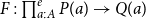 $F:\prod ^e_{a:A} P(a) \to Q(a)$
where each
$F:\prod ^e_{a:A} P(a) \to Q(a)$
where each
 $F(a)$
is an equivalence, then fibrant matches of
$F(a)$
is an equivalence, then fibrant matches of
 $\prod ^e_{a:A} P(a)$
and
$\prod ^e_{a:A} P(a)$
and
 $\prod ^e_{a:A} Q(a)$
are also equivalent.
$\prod ^e_{a:A} Q(a)$
are also equivalent.

The definition being a sharp exo-type.

An example of Agda’s different behaviors about level checking.

As noted in Remark 2.28, we keep a second copy of the library, 2LTT_C, which is compiled without the –cumulativity flag. Except for a few low-level details, the two code bases are line-for-line identical, so all results in this paper carry over verbatim. The flag does, however, affect universe inference. When –cumulativity is off, the checker can almost always infer the required universe levels automatically. With the flag on, the same term may yield an UnsolvedConstraints error, forcing the user to spell out the levels by hand. Agda Code 11 illustrates the difference: the first definition type-checks in 2LTT_C; in 2LTT we must supply the explicit level parameters for each isEquiv witness and for the equivalence type
 $\_\simeq \_$
.
$\_\simeq \_$
.
The 2LTT and 2LTT_C repositories together provide a complete, flag-parametrized formalization of every concept used in this paper: two-level universes, main type-formers, and the three structural classes (fibrant, cofibrant, and sharp exo-types). Both variants compile cleanly with Agda 2.8.0 and the standard library 2.2, and all theorems cited here are verified verbatim. Upcoming work will enrich the code base with the semantics of diagram signatures and further results of 2LTT, but the current release already stands as a stable reference implementation for the theory developed in this article.
3. Two-level type theory - semantics
In this section, we will examine the semantic aspect of the theory discussed in the previous sections. In order for the axioms we accept about natural numbers to have meaning, we will investigate their models, preferably a large number of them. To do this, we will first provide the necessary background information about the models of the two-level type theory and then introduce the additional conditions required to fulfill the aforementioned axiom. As in the previous section, we omit the proofs unless the result is novel to the study.
During this section, we follow the conventions below.
Variables.
 $\Gamma$
,
$\Gamma$
,
 $\Delta$
,
$\Delta$
,
 $\ldots$
stand for contexts,
$\ldots$
stand for contexts,
 $\sigma$
,
$\sigma$
,
 $\theta$
,
$\theta$
,
 $\tau$
,
$\tau$
,
 $\ldots$
for context morphisms,
$\ldots$
for context morphisms,
 $P$
,
$P$
,
 $Q$
,
$Q$
,
 $R$
,
$R$
,
 $\ldots$
for presheaves,
$\ldots$
for presheaves,
 $A$
,
$A$
,
 $B$
,
$B$
,
 $C$
,
$C$
,
 $Y$
,
$Y$
,
 $\ldots$
for types and type families, and
$\ldots$
for types and type families, and
 $a$
,
$a$
,
 $b$
,
$b$
,
 $c$
,
$c$
,
 $\ldots$
for terms.
$\ldots$
for terms.
Substitution. Whenever
 $P : \mathcal{C}^{\textrm {{op}}} \rightarrow {\mathsf{Set}}$
is a presheaf,
$P : \mathcal{C}^{\textrm {{op}}} \rightarrow {\mathsf{Set}}$
is a presheaf,
 $\sigma : \Delta \rightarrow \Gamma$
a morphism, and
$\sigma : \Delta \rightarrow \Gamma$
a morphism, and
 $A : P(\Gamma )$
, we write
$A : P(\Gamma )$
, we write
 $A[\sigma ]$
instead of
$A[\sigma ]$
instead of
 $P(\sigma )(A)$
.
$P(\sigma )(A)$
.
Equality signs. Recall that 2LTT has two different equality signs: “
 $\mathsf{=}^{\textit {e}}$
” and “
$\mathsf{=}^{\textit {e}}$
” and “
 $=$
”. Now, another equality comes forward, and that is equality in meta-theory. We reserve “
$=$
”. Now, another equality comes forward, and that is equality in meta-theory. We reserve “
 $=$
” for the meta-theory’s equality and use “
$=$
” for the meta-theory’s equality and use “
 $\mathsf{Id}$
” for the identity type “
$\mathsf{Id}$
” for the identity type “
 $\mathsf{Eq}$
” for the exo-equality.
$\mathsf{Eq}$
” for the exo-equality.
3.1 Review
Common models of type theories arise in the category with families. A category with families (CwF) consists of the following:
-
• A category
$\mathcal{C}$
with a terminal object
$ 1_{\mathcal{C}} : \mathcal{C}$
. Its objects are called contexts, and
$1_{\mathcal{C}}$
is called the empty context. -
• A presheaf
$\texttt {Ty} : \mathcal{C}^{\textrm {{op}}} \rightarrow {\mathsf{Set}}$
. If
$ A : \texttt {Ty}(\Gamma )$
, then we say
$A$
is a type over
$\Gamma$
. -
• A presheaf
$\texttt {Tm} : (\!\int \texttt {Ty})^{\textrm {{op}}} \rightarrow {\mathsf{Set}}$
. If
$a : \texttt {Tm}(\Gamma , A)$
, then we say
$a$
is a term of
$A$
. -
• For any
$\Gamma : \mathcal{C}$
and
$A : \texttt {Ty}(\Gamma )$
, there is an object
$\Gamma .A :\mathcal{C}$
, a morphism
$p_A : \Gamma .A \rightarrow \Gamma$
, and a term
$q_A : \texttt {Tm}(\Gamma .A,A[p_A])$
with the universal property: for any object
$\Delta : \mathcal{C}$
, a morphism
$\sigma : \Delta \rightarrow \Gamma$
, and a term
$a:\texttt {Tm}(\Delta ,A[\sigma ])$
, there is a unique morphism
$\theta : \Delta \rightarrow \Gamma .A$
such that
$p_A \circ \theta = \sigma$
and
$q_A[\theta ]=a$
. This operation is called the context extension.


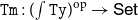


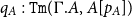


Note that for all contexts
 $\Gamma : \mathcal{C}$
and types
$\Gamma : \mathcal{C}$
and types
 $A : \texttt {Ty}(\Gamma )$
, there is a natural isomorphism
$A : \texttt {Ty}(\Gamma )$
, there is a natural isomorphism
 \begin{equation*}\texttt {Tm}(\Gamma ,A)\cong \mathcal{C}/{\Gamma }((\Gamma ,\mathsf{id}_{\Gamma }),(\Gamma .A,p_A)).\end{equation*}
Indeed, this follows from the universal property of the context extension by taking
 $\Delta \;:=\;\Gamma$
and
$\Delta \;:=\;\Gamma$
and
 $\sigma \;:=\;\mathsf{id}_{\Gamma }$
. This observation says that the terms of
$\sigma \;:=\;\mathsf{id}_{\Gamma }$
. This observation says that the terms of
 $A$
over
$A$
over
 $\Gamma$
can be regarded as the sections of
$\Gamma$
can be regarded as the sections of
 $p_A:\Gamma .A \rightarrow \Gamma$
.
$p_A:\Gamma .A \rightarrow \Gamma$
.
The proposition below is a useful fact for the rest of the section.
Proposition 3.1.
Let
 $\sigma :\Delta \rightarrow \Gamma$
be a context morphism and
$\sigma :\Delta \rightarrow \Gamma$
be a context morphism and
 $A:\texttt {Ty}(\Gamma )$
. There exists a morphism
$A:\texttt {Ty}(\Gamma )$
. There exists a morphism
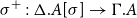 $\sigma ^{+}:\Delta .A[\sigma ] \rightarrow \Gamma .A$
that makes the following diagram into a pullback square:
$\sigma ^{+}:\Delta .A[\sigma ] \rightarrow \Gamma .A$
that makes the following diagram into a pullback square:

Rather than presenting a specific instance of a CwF, we will offer a more extensive range of CwF examples. The category of presheaves is an archetypal example of a CwF (Hofmann, Reference Hofmann1997). Let
 $\mathcal{C}$
be a (small) category, and let
$\mathcal{C}$
be a (small) category, and let
 $\widehat {\mathcal{C}}$
be its category of presheaves. The CwF structure on
$\widehat {\mathcal{C}}$
be its category of presheaves. The CwF structure on
 $\widehat {\mathcal{C}}$
, denoted by
$\widehat {\mathcal{C}}$
, denoted by
 $(\widehat {\texttt {Ty}}, \widehat {\texttt {Tm}})$
is defined in the following manner:
$(\widehat {\texttt {Ty}}, \widehat {\texttt {Tm}})$
is defined in the following manner:
-
• Contexts are presheaves
$\mathcal{C}^{\textrm {{op}}} \rightarrow {\mathsf{Set}}$
. -
• The constant presheaf that takes the value
$\star$
in the category of sets can be characterized as the terminal object
$1_{\widehat {\mathcal{C}}}$
. -
• Recall that
$\widehat {\texttt {Ty}}$
is a presheaf on
$\widehat {\mathcal{C}}$
.If
$P:\widehat {\mathcal{C}}$
, then
$\widehat {\texttt {Ty}}(P)$
is the underlying set of the category of presheaves
$\widehat {\int P}$
over the category of elements
$\int P$
. In other words, a type
$A:\widehat {\texttt {Ty}}(P)$
is a functor
$\left (\int P \right )^{\textrm {{op}}} \rightarrow {\mathsf{Set}}$
.If
$\phi :Q \rightarrow P$
is a morphism in
$\widehat {\mathcal{C}}$
and
$A:\widehat {\texttt {Ty}}(P)$
, we define the type substitution
$A[\phi ]:\widehat {\texttt {Ty}}(Q)$
aswhere
\begin{equation*}A[\phi ](\Gamma ,x)\;:=\; A (\Gamma ,\phi _{\Gamma }(x))\end{equation*}
$x:Q_{\Gamma }$
.
-
• Recall that
$\widehat {\texttt {Tm}}$
is a presheaf on
$\int \widehat {\texttt {Ty}}$
.For
$P:\widehat {\mathcal{C}}$
and
$A:\widehat {\texttt {Ty}}(P)$
, we define
\begin{equation*}\widehat {\texttt {Tm}}(P,A) \;:=\; \left \lbrace a : \prod _{\Gamma : \mathcal{C},\, x: P_{\Gamma }} A(\Gamma ,x) \mid \text{ if } \sigma : \Delta \rightarrow \Gamma , \, x : P_{\Gamma }\text{, then } a(\Gamma ,x)[\sigma ]=a(\Delta ,x[\sigma ])\right \rbrace .\end{equation*}
If
$\phi :Q \rightarrow P$
is a morphism in
$\widehat {\mathcal{C}}$
,
$A:\widehat {\texttt {Ty}}(P)$
, and
$a:\widehat {\texttt {Tm}}(P,A)$
, we define the term substitution
$a[\phi ]:\widehat {\texttt {Tm}}(Q,A[\phi ])$
aswhere
\begin{equation*}a[\phi ](\Gamma ,x)\;:=\; a (\Gamma ,\phi _{\Gamma }(x))\end{equation*}
$x:Q_{\Gamma }$
.
-
• For
$P:\widehat {\mathcal{C}}$
and
$A:\widehat {\texttt {Ty}}(P)$
, the context
$P.A$
is again a presheaf over
$\mathcal{C}$
defined by
\begin{equation*}P.A(\Gamma )\;:=\;\prod_{x : P(\Gamma )} A(\Gamma , x).\end{equation*}
If
$\sigma : \Delta \rightarrow \Gamma$
is a morphism in
$\mathcal{C}$
and
$(x,a):P.A (\Gamma )$
, then we define
\begin{equation*}(x,a)[\sigma ]=P.A(\sigma ) (x,a)\;:=\;(x[\sigma ],a[\sigma ]).\end{equation*}
The morphism
$p_A:P.A \rightarrow P$
is defined by the first projection. In other words, for
$\Gamma : \mathcal{C}$
and
$(x ,a): P.A(\Gamma )$
, we have
$(p_A)_{\Gamma }(x,a)=x$
. The term
$q_A: \widehat {\texttt {Tm}}(P.A,A[p_A])$
is given by the second projection. In other words, for
$\Gamma :\mathcal{C}$
and
$(x,a): P.A(\Gamma )$
, we have
$q_A(\Gamma , (x,a))=a$
. Note that
$A[p_A](\Gamma ,(x,a))=A(\Gamma ,p_A(x,a))=A(\Gamma ,x)$
.It remains to verify the universal property for the context extension.
Let
$Q:\widehat {\mathcal{C}}$
,
$\tau :Q\rightarrow P$
, and
$b:\widehat {\texttt {Tm}}(Q,A[\tau ])$
. Define
$\theta :Q \rightarrow P.A$
as follows: for
$\Gamma : \mathcal{C}$
and
$x:Q_{\Gamma }$
, we haveIt is straightforward to verify the defining rules:
\begin{equation*}\theta _{\Gamma }(x)\;:=\; (\tau _{\Gamma }(x),b(\Gamma ,x)).\end{equation*}
$p_A\circ \theta =\tau$
becauseand
\begin{equation*}(p_A\circ \theta )_{\Gamma }(x)=p_A(\tau _{\Gamma }(x),b(\Gamma ,x))=\tau _{\Gamma }(x),\end{equation*}
$q_A[\theta ]=b$
becauseSince the defining properties of
\begin{equation*}q_A[\theta ](\Gamma ,x)=q_A(\Gamma , \theta _{\Gamma }(x))=q_A(\Gamma , (\tau _{\Gamma }(x),b(\Gamma ,x)))=b(\Gamma ,x).\end{equation*}
$p_A$
and
$q_A$
determine the map
$\theta$
, it is uniquely determined.


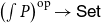


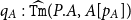


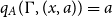


Another well-known example is the category
 $\mathsf{SSet}$
. Let
$\mathsf{SSet}$
. Let
 $\mathcal{C}=\bigtriangleup$
be the simplex category. The presheaf category
$\mathcal{C}=\bigtriangleup$
be the simplex category. The presheaf category
 $\widehat {\bigtriangleup }$
is called the category of simplicial sets, denoted by
$\widehat {\bigtriangleup }$
is called the category of simplicial sets, denoted by
 $\mathsf{SSet}$
. Like any other presheaf category,
$\mathsf{SSet}$
. Like any other presheaf category,
 $\mathsf{SSet}$
has a CwF structure
$\mathsf{SSet}$
has a CwF structure
 $(\widehat {\texttt {Ty}},\widehat {\texttt {Tm}})$
, but it has another CwF structure. We only define a new type presheaf
$(\widehat {\texttt {Ty}},\widehat {\texttt {Tm}})$
, but it has another CwF structure. We only define a new type presheaf
 $\texttt {Ty} : {\mathsf{SSet}}^{\textrm {{op}}} \rightarrow {\mathsf{Set}}$
as follows:
$\texttt {Ty} : {\mathsf{SSet}}^{\textrm {{op}}} \rightarrow {\mathsf{Set}}$
as follows:
 $\texttt {Ty}(P)$
is a subset of
$\texttt {Ty}(P)$
is a subset of
 $\widehat {\texttt {Ty}}(P)$
such that
$\widehat {\texttt {Ty}}(P)$
such that
 $A : \texttt {Ty}(P)$
if the display map
$A : \texttt {Ty}(P)$
if the display map
 $P.A \rightarrow P$
is a Kan fibration. With the induced term presheaf
$P.A \rightarrow P$
is a Kan fibration. With the induced term presheaf
 $\texttt {Tm}$
obtained by
$\texttt {Tm}$
obtained by
 $\widehat {\texttt {Tm}}$
, we obtain a CwF
$\widehat {\texttt {Tm}}$
, we obtain a CwF
 $({\mathsf{SSet}}, \texttt {Ty}, \texttt {Tm})$
. It is easy to prove this structure satisfies all axioms of being a CwF (Capriotti, Reference Capriotti2016). We always refer to this new CwF structure on
$({\mathsf{SSet}}, \texttt {Ty}, \texttt {Tm})$
. It is easy to prove this structure satisfies all axioms of being a CwF (Capriotti, Reference Capriotti2016). We always refer to this new CwF structure on
 $\mathsf{SSet}$
unless stated otherwise.
$\mathsf{SSet}$
unless stated otherwise.
 $\mathsf{SSet}$
is not a unique example of a presheaf category having two CwF structures. There are many of them, and they will be useful to talk about two-level structures in the later sections.
$\mathsf{SSet}$
is not a unique example of a presheaf category having two CwF structures. There are many of them, and they will be useful to talk about two-level structures in the later sections.
Now, we need to establish the meanings of particular type formers within a CwF and to examine the requirements that must be fulfilled for the CwF to possess these type formers. Although this analysis could be applied to various standard type formers, our focus will be solely on those indispensable for the rest of the study. One can see the definitions of type formers in a CwF from (Hofmann, Reference Hofmann1997) and (Uskuplu, Reference Uskuplu2023). We only provide what they mean in a presheaf CwF.
We start with the
 $\Pi$
types in a presheaf Cwf.
$\Pi$
types in a presheaf Cwf.
Let
 $A:\widehat {\texttt {Ty}}(P)$
and
$A:\widehat {\texttt {Ty}}(P)$
and
 $B:\widehat {\texttt {Ty}}(P.A)$
. First, we need to define
$B:\widehat {\texttt {Ty}}(P.A)$
. First, we need to define
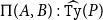 $\Pi (A,B):\widehat {\texttt {Ty}}(P)$
. Recall that
$\Pi (A,B):\widehat {\texttt {Ty}}(P)$
. Recall that
 $\Pi (A,B)$
should be a presheaf over
$\Pi (A,B)$
should be a presheaf over
 $\int P$
. For each
$\int P$
. For each
 $\Gamma :\mathcal{C}$
and
$\Gamma :\mathcal{C}$
and
 $x:P_{\Gamma }$
, the type
$x:P_{\Gamma }$
, the type
 $\Pi (A,B)(\Gamma ,x)$
consists of the elements
$\Pi (A,B)(\Gamma ,x)$
consists of the elements
 $f$
in the categorical product
$f$
in the categorical product
 \begin{equation*} f: \mathbf{\prod }_{\Delta :\mathcal{C},\, \sigma :\Delta \rightarrow \Gamma ,\, a: A (\Delta , x[\sigma ])} B(\Delta , (x[\sigma ],a)) \end{equation*}
such that if
 $\Theta : \mathcal{C}$
and
$\Theta : \mathcal{C}$
and
 $\tau : \Theta \rightarrow \Delta$
, then
$\tau : \Theta \rightarrow \Delta$
, then
 \begin{equation} f(\Delta ,\sigma ,a)[\tau ]=f(\Theta ,\sigma \circ \tau ,a[\tau ]). \end{equation}
If
 $\tau :(\Upsilon ,y)\rightarrow (\Gamma ,x)$
is a morphism in
$\tau :(\Upsilon ,y)\rightarrow (\Gamma ,x)$
is a morphism in
 $\int P$
, namely,
$\int P$
, namely,
 $\tau : \Upsilon \rightarrow \Gamma$
is a morphism in
$\tau : \Upsilon \rightarrow \Gamma$
is a morphism in
 $\mathcal{C}$
such that
$\mathcal{C}$
such that
 $x[\tau ]=y$
, for each
$x[\tau ]=y$
, for each
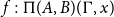 $f : \Pi (A,B)(\Gamma ,x)$
,
$f : \Pi (A,B)(\Gamma ,x)$
,
 $\Delta : \mathcal{C}$
,
$\Delta : \mathcal{C}$
,
 $\sigma : \Delta \rightarrow \Upsilon$
, and
$\sigma : \Delta \rightarrow \Upsilon$
, and
 $a : A (\Delta , y[\sigma ])$
, we define
$a : A (\Delta , y[\sigma ])$
, we define
 $f[\tau ](\Delta ,\sigma ,a)\;:=\;f(\Delta , \tau \circ \sigma , a)$
. Using the compatibility condition 5, we indeed obtain a presheaf
$f[\tau ](\Delta ,\sigma ,a)\;:=\;f(\Delta , \tau \circ \sigma , a)$
. Using the compatibility condition 5, we indeed obtain a presheaf
 $\Pi (A,B)$
on
$\Pi (A,B)$
on
 $\int P$
.
$\int P$
.
Second, for each
 $b:\widehat {\texttt {Tm}}(P.A,B)$
, we need to define a term
$b:\widehat {\texttt {Tm}}(P.A,B)$
, we need to define a term
 $\lambda (b):\widehat {\texttt {Tm}}(P,\Pi (A,B))$
. Recall that
$\lambda (b):\widehat {\texttt {Tm}}(P,\Pi (A,B))$
. Recall that
 $\lambda (b)$
should be an element in
$\lambda (b)$
should be an element in
 \begin{equation*}\mathbf{\prod }_{\Gamma : \mathcal{C}, x : P_{\Gamma }} \Pi (A,B)(\Gamma ,x).\end{equation*}
Now, for
 $\Gamma :\mathcal{C}$
,
$\Gamma :\mathcal{C}$
,
 $x : P_{\Gamma }$
,
$x : P_{\Gamma }$
,
 $\Delta :\mathcal{C}$
,
$\Delta :\mathcal{C}$
,
 $\sigma :\Delta \rightarrow \Gamma$
, and
$\sigma :\Delta \rightarrow \Gamma$
, and
 $a : A(\Delta , x[\sigma ])$
we define
$a : A(\Delta , x[\sigma ])$
we define
 \begin{equation*}\lambda (b)(\Gamma ,x) (\Delta ,\sigma ,a)\;:=\;b(\Delta ,x[\sigma ],a).\end{equation*}
This definition makes sense because the term
 $b$
is in
$b$
is in
 $\mathbf{\prod }_{\Gamma : \mathcal{C}, z : P.A_{\Gamma }} B(\Gamma ,z)$
.
$\mathbf{\prod }_{\Gamma : \mathcal{C}, z : P.A_{\Gamma }} B(\Gamma ,z)$
.
Third, for each
 $f:\widehat {\texttt {Tm}}(P,\Pi (A,B))$
and
$f:\widehat {\texttt {Tm}}(P,\Pi (A,B))$
and
 $a:\widehat {\texttt {Tm}}(P,A)$
, we need to define a term
$a:\widehat {\texttt {Tm}}(P,A)$
, we need to define a term
 ${\mathsf{app}}(f,a):\widehat {\texttt {Tm}}(P,B[a])$
. Recall that it should be in
${\mathsf{app}}(f,a):\widehat {\texttt {Tm}}(P,B[a])$
. Recall that it should be in
 \begin{equation*}\mathbf{\prod }_{\Gamma : \mathcal{C}, x : P_{\Gamma }} B[a](\Gamma ,x).\end{equation*}
Now, for
 $\Gamma :\mathcal{C}$
,
$\Gamma :\mathcal{C}$
,
 $x : P_{\Gamma }$
, we define
$x : P_{\Gamma }$
, we define
 \begin{equation*}{\mathsf{app}}(f,a)(\Gamma ,x)\;:=\; f(\Gamma ,x)(\Gamma ,\mathsf{id},a).\end{equation*}
Next, we provide
 $\Sigma$
types in terms of the presheaf CwFs.
$\Sigma$
types in terms of the presheaf CwFs.
Let
 $A:\widehat {\texttt {Ty}}(P)$
and
$A:\widehat {\texttt {Ty}}(P)$
and
 $B:\widehat {\texttt {Ty}}(P.A)$
. First, we need to define
$B:\widehat {\texttt {Ty}}(P.A)$
. First, we need to define
 $\Sigma (A,B):\widehat {\texttt {Ty}}(P)$
. Recall that
$\Sigma (A,B):\widehat {\texttt {Ty}}(P)$
. Recall that
 $\Sigma (A,B)$
should be a presheaf over
$\Sigma (A,B)$
should be a presheaf over
 $\int P$
. For each
$\int P$
. For each
 $\Gamma :\mathcal{C}$
and
$\Gamma :\mathcal{C}$
and
 $x:P_{\Gamma }$
, we define
$x:P_{\Gamma }$
, we define
 \begin{equation*}\Sigma (A,B)(\Gamma ,x)\;:=\;\lbrace (a,b) |\, a : A(\Gamma ,x),\, b: B(\Gamma ,(x,a)) \rbrace . \end{equation*}
For a morphism
 $\sigma : (\Delta ,y)\rightarrow (\Gamma ,x)$
in
$\sigma : (\Delta ,y)\rightarrow (\Gamma ,x)$
in
 $\int P$
and
$\int P$
and
 $(a,b):\Sigma (A,B)(\Gamma ,x)$
, we define
$(a,b):\Sigma (A,B)(\Gamma ,x)$
, we define
 \begin{equation*}(a,b)[\sigma ]\;:=\;(a[\sigma ],b[\sigma ]).\end{equation*}
One can define the operations
 $\langle \_,\_ \rangle$
,
$\langle \_,\_ \rangle$
,
 $\pi _1$
, and
$\pi _1$
, and
 $\pi _2$
in an obvious way, and it is easy to prove the coherence rules.
$\pi _2$
in an obvious way, and it is easy to prove the coherence rules.
Thirdly, the presheaf CwFs also satisfy the extensional identities.
Let
 $A:\widehat {\texttt {Ty}}(P)$
. Recall that
$A:\widehat {\texttt {Ty}}(P)$
. Recall that
 ${\mathsf{Eq}}_A$
should be a presheaf over
${\mathsf{Eq}}_A$
should be a presheaf over
 $\int \Gamma .A.A[p_A]$
. For each
$\int \Gamma .A.A[p_A]$
. For each
 $\Gamma :\mathcal{C}$
,
$\Gamma :\mathcal{C}$
,
 $x:P_{\Gamma }$
, and
$x:P_{\Gamma }$
, and
 $a,b: A(\Gamma ,x)$
, we define
$a,b: A(\Gamma ,x)$
, we define
 \begin{equation*}{\mathsf{Eq}}_A(\Gamma ,x,a,b)\;:=\; \begin{cases} \{\star \} & \text{if } a = b\\ \emptyset & \text{if } a \neq b \end{cases}.\end{equation*}
The morphism
 ${\mathsf{refl}}^e_A : P.A \rightarrow P.A.A[p_A].{\mathsf{Eq}}_A$
is defined for each
${\mathsf{refl}}^e_A : P.A \rightarrow P.A.A[p_A].{\mathsf{Eq}}_A$
is defined for each
 $\Gamma : \mathcal{C}$
as
$\Gamma : \mathcal{C}$
as
 $(x,a) \mapsto (x,a,a,\star )$
. Since
$(x,a) \mapsto (x,a,a,\star )$
. Since
 $p_{{\mathsf{Eq}}}: P.A.A[p_A].{\mathsf{Eq}}_A \rightarrow P.A.A[p_A]$
is the first projection, we indeed have
$p_{{\mathsf{Eq}}}: P.A.A[p_A].{\mathsf{Eq}}_A \rightarrow P.A.A[p_A]$
is the first projection, we indeed have
 $p_{{\mathsf{Eq}}}\circ {\mathsf{refl}}^e_A$
is the diagonal map.
$p_{{\mathsf{Eq}}}\circ {\mathsf{refl}}^e_A$
is the diagonal map.
If
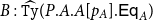 $B : \widehat {\texttt {Ty}}(P.A.A[p_A].{\mathsf{Eq}}_A)$
, the function
$B : \widehat {\texttt {Ty}}(P.A.A[p_A].{\mathsf{Eq}}_A)$
, the function
 $J^e:\widehat {\texttt {Tm}}(P.A, B[{\mathsf{refl}}^e_A]) \rightarrow \widehat {\texttt {Tm}}(P.A.A[p_A].{\mathsf{Eq}}_A, B)$
is defined as follows: If
$J^e:\widehat {\texttt {Tm}}(P.A, B[{\mathsf{refl}}^e_A]) \rightarrow \widehat {\texttt {Tm}}(P.A.A[p_A].{\mathsf{Eq}}_A, B)$
is defined as follows: If
 $\alpha : \widehat {\texttt {Tm}}(P.A, B[{\mathsf{refl}}^e_A])$
, this means we have
$\alpha : \widehat {\texttt {Tm}}(P.A, B[{\mathsf{refl}}^e_A])$
, this means we have
 \begin{equation*}\alpha : \prod _{\substack {\Gamma : \mathcal{C} \\ (x,a): P.A_{\Gamma }}} B(\Gamma ,(x,a,a,\star ))\quad \text{ and } \quad J^e(\alpha ) : \prod _{\substack {\Gamma : \mathcal{C}\\ (x,a,b,p): P.A.A[p_A].{\mathsf{Eq}}_{\Gamma }}} B(\Gamma ,(x,a,b,p)).\end{equation*}
Thus, we define
 $J^e(\alpha )(\Gamma ,(x,a,b,p))\;:=\;\alpha (\Gamma ,(x,a))$
, which makes sense because
$J^e(\alpha )(\Gamma ,(x,a,b,p))\;:=\;\alpha (\Gamma ,(x,a))$
, which makes sense because
 $p : {\mathsf{Eq}}(a,b)$
means
$p : {\mathsf{Eq}}(a,b)$
means
 $a=b$
and
$a=b$
and
 $p=\star$
. It is easy to prove the coherence rules.
$p=\star$
. It is easy to prove the coherence rules.
Since the intensional identity type former,
 $\mathsf{Id}$
, is a particular case of
$\mathsf{Id}$
, is a particular case of
 $\mathsf{Eq}$
, we can say that every presheaf CwF supports intensional identity types. If we also assume univalence for intensional identities, it is not true in general that every presheaf CwF supports such an identity. For example, the presheaf CwF on
$\mathsf{Eq}$
, we can say that every presheaf CwF supports intensional identity types. If we also assume univalence for intensional identities, it is not true in general that every presheaf CwF supports such an identity. For example, the presheaf CwF on
 $\mathsf{Set}$
supports the identity type and the uniqueness of identity proof (UIP), but UIP contradicts with univalence (HoTTBook, 2013). Nonetheless, it has been established that the simplicial set CwF, denoted as
$\mathsf{Set}$
supports the identity type and the uniqueness of identity proof (UIP), but UIP contradicts with univalence (HoTTBook, 2013). Nonetheless, it has been established that the simplicial set CwF, denoted as
 $\mathsf{SSet}$
, does provide support for univalent identity types (Kapulkin and Lumsdaine, Reference Kapulkin and Lumsdaine2021). Indeed, this category stands as one of the widely recognized models not only for Martin-Löf Type Theory but also for Homotopy Type Theory.
$\mathsf{SSet}$
, does provide support for univalent identity types (Kapulkin and Lumsdaine, Reference Kapulkin and Lumsdaine2021). Indeed, this category stands as one of the widely recognized models not only for Martin-Löf Type Theory but also for Homotopy Type Theory.
In the case of intensional identity types, we can also establish a definition for what constitutes a “contractible” type. This notion serves as a crucial component in the overall definition of cofibrancy.
Definition 3.2.
Let
 $A:\texttt {Ty}(\Gamma )$
be a type. We call
$A:\texttt {Ty}(\Gamma )$
be a type. We call
 $A$
a contractible type if there is a term in the following type over
$A$
a contractible type if there is a term in the following type over
 $\Gamma$
:
$\Gamma$
:
 \begin{equation*}{\mathsf{isContr}}(A)\;:=\;\Sigma (A,\Pi (A[p_A],\mathsf{Id}_A)).\end{equation*}
Having such a term means that there is a term
 $c : \texttt {Tm}(\Gamma ,A)$
called center of contraction, such that for any term
$c : \texttt {Tm}(\Gamma ,A)$
called center of contraction, such that for any term
 $a: \texttt {Tm}(\Gamma .A,A[p_A])$
there is a term
$a: \texttt {Tm}(\Gamma .A,A[p_A])$
there is a term
 $p: \texttt {Tm}(\Gamma ,\mathsf{Id}_A[c^+,a^+])$
. In other words, we have a section map
$p: \texttt {Tm}(\Gamma ,\mathsf{Id}_A[c^+,a^+])$
. In other words, we have a section map
 $c:\Gamma \rightarrow \Gamma .A$
to
$c:\Gamma \rightarrow \Gamma .A$
to
 $p_A$
such that the following diagram, where
$p_A$
such that the following diagram, where
 $h$
is the contracting homotopy commutes:
$h$
is the contracting homotopy commutes:

Finally, we will show that for any (small) category
 $\mathcal{C}$
, the presheaf Cwf
$\mathcal{C}$
, the presheaf Cwf
 $(\widehat {\mathcal{C}},\widehat {\texttt {Ty}},\widehat {\texttt {Tm}})$
supports a natural number type.
$(\widehat {\mathcal{C}},\widehat {\texttt {Ty}},\widehat {\texttt {Tm}})$
supports a natural number type.
Since
 $\mathbb{N}$
should be a presheaf over
$\mathbb{N}$
should be a presheaf over
 $\int 1_{\widehat {C}}$
, for each
$\int 1_{\widehat {C}}$
, for each
 $\Gamma :\mathcal{C}$
and
$\Gamma :\mathcal{C}$
and
 $x:(1_{\widehat {C}})_{\Gamma }$
we define
$x:(1_{\widehat {C}})_{\Gamma }$
we define
 $\mathbb{N}(\Gamma ,x)\;:=\; \mathbf{N}$
, the external set of natural numbers. The term
$\mathbb{N}(\Gamma ,x)\;:=\; \mathbf{N}$
, the external set of natural numbers. The term
 ${\mathsf{0}} : \widehat {\texttt {Tm}}(1_{\widehat {C}}, \mathbb{N})$
is obtained by the morphism
${\mathsf{0}} : \widehat {\texttt {Tm}}(1_{\widehat {C}}, \mathbb{N})$
is obtained by the morphism
 $1_{\widehat {C}} \rightarrow 1_{\widehat {C}}.\mathbb{N}$
which we define
$1_{\widehat {C}} \rightarrow 1_{\widehat {C}}.\mathbb{N}$
which we define
 ${\mathsf{0}}_{\Gamma }(x)\;:=\;(x,0)$
for any
${\mathsf{0}}_{\Gamma }(x)\;:=\;(x,0)$
for any
 $\Gamma :\mathcal{C}$
and
$\Gamma :\mathcal{C}$
and
 $x:(1_{\widehat {C}})_{\Gamma }$
. The morphism
$x:(1_{\widehat {C}})_{\Gamma }$
. The morphism
 ${\mathsf{succ}}:1_{\widehat {C}}.\mathbb{N} \rightarrow 1_{\widehat {C}}.\mathbb{N}$
is defined as
${\mathsf{succ}}:1_{\widehat {C}}.\mathbb{N} \rightarrow 1_{\widehat {C}}.\mathbb{N}$
is defined as
 ${\mathsf{succ}}_{\Gamma }(x,k)\;:=\;(x, k+1)$
for any
${\mathsf{succ}}_{\Gamma }(x,k)\;:=\;(x, k+1)$
for any
 $\Gamma :\mathcal{C}$
and
$\Gamma :\mathcal{C}$
and
 $(x,k):(1_{\widehat {C}}.\mathbb{N})_{\Gamma }$
.
$(x,k):(1_{\widehat {C}}.\mathbb{N})_{\Gamma }$
.
For any
 $P :\widehat {\mathcal{C}}$
and
$P :\widehat {\mathcal{C}}$
and
 $\sigma : P \rightarrow 1_{\widehat {\mathcal{C}}}$
, if
$\sigma : P \rightarrow 1_{\widehat {\mathcal{C}}}$
, if
 $B : \widehat {\texttt {Ty}}(P.\mathbb{N}[\sigma ])$
with
$B : \widehat {\texttt {Ty}}(P.\mathbb{N}[\sigma ])$
with
 $b_0$
and
$b_0$
and
 $b_s$
, the function
$b_s$
, the function
 $J^{\mathbb{N}}_B:P.\mathbb{N}[\sigma ] \rightarrow P.\mathbb{N}[\sigma ].B$
is defined as, for each
$J^{\mathbb{N}}_B:P.\mathbb{N}[\sigma ] \rightarrow P.\mathbb{N}[\sigma ].B$
is defined as, for each
 $\Gamma :\mathcal{C}$
, and
$\Gamma :\mathcal{C}$
, and
 $(x,k):(P.\mathbb{N}[\sigma ])_{\Gamma }$
 \begin{equation*}(J^{\mathbb{N}}_B)_{\Gamma }(x,k)\;:=\; \begin{cases} {b_0(x)} & \text{if } k = 0\\ {b_s\big ((x,k'),\,(J^{\mathbb{N}}_B)_{\Gamma }(x,k')\big )} & \text{if } k = k' + 1 \end{cases}.\end{equation*}
Clearly,
 $J^{\mathbb{N}}_B \circ {\mathsf{0}}[\sigma ]=b_0$
holds. For the other equality, we have
$J^{\mathbb{N}}_B \circ {\mathsf{0}}[\sigma ]=b_0$
holds. For the other equality, we have
 \begin{equation*}(J^{\mathbb{N}}_B \circ {\mathsf{succ}}[\sigma ])_{\Gamma }(x,k)=(J^{\mathbb{N}}_B)_{\Gamma }(x,k+1)=(b_s)_{\Gamma }\big ((x,k),\,(J^{\mathbb{N}}_B)_{\Gamma }(x,k)\big ).\end{equation*}
Also, it is easy to prove the remaining coherence rules.
Remark 3.3. We can talk about the unit type, the empty type, coproducts, and others and give the conditions for a CwF to support them. In general, if we have a collection
 $T$
of type formers, we say a CwF supports
$T$
of type formers, we say a CwF supports
 $T$
if the CwF supports each type formers in
$T$
if the CwF supports each type formers in
 $T$
.
$T$
.
Example 3.4.
Let
 $T\;:=\;\{\prod , \sum , {\mathbf{1}}, {\mathbf{0}}, \mathbb{N}, {\mathsf{Eq}}\}$
. Then a presheaf CwF
$T\;:=\;\{\prod , \sum , {\mathbf{1}}, {\mathbf{0}}, \mathbb{N}, {\mathsf{Eq}}\}$
. Then a presheaf CwF
 $(\widehat {\mathcal{C}},\widehat {\texttt {Ty}},\widehat {\texttt {Tm}})$
supports
$(\widehat {\mathcal{C}},\widehat {\texttt {Ty}},\widehat {\texttt {Tm}})$
supports
 $T$
.Footnote
8
$T$
.Footnote
8
Based on the example of presheaf CwF we discussed earlier, it becomes clear that CwFs can be used to model dependent type theory. A CwF provides a structure that covers contexts, types, terms, and substitutions. Moreover, if a CwF has enough type formers, it allows us to work with dependent products, dependent sums, and other inductive types. If you’re interested in delving into the details and exploring similar constructions related to CwFs, you can refer to Capriotti (Reference Capriotti2016). Our primary focus here is to establish the necessary background to discuss models where exo-nat is cofibrant.
Definition 3.5 (Annenkov et al., Reference Annenkov, Capriotti, Kraus and Sattler2023). A model of Martin-Löf type theory with type formers
 $T$
is a CwF that supports
$T$
is a CwF that supports
 $T$
.
$T$
.
We already know that a presheaf CwF is a model of Martin-Löf type theory with usual type formers and extensional identity types. The simplicial set CwF
 $\mathsf{SSet}$
is a model of Martin-Löf type theory with usual type formers and intensional identity types.
$\mathsf{SSet}$
is a model of Martin-Löf type theory with usual type formers and intensional identity types.
Let us recall that this study on semantics aims to gain insight into the models of 2LTT with a cofibrant exo-nat. Once we have acquired models of various type theories, a natural question arises: can we merge these models to obtain a comprehensive model of 2LTT? The answer to this question is affirmative, as it is indeed possible to combine two CwF structures in the same category in a manner that ensures their compatibility and coherence.
Definition 3.6 (Capriotti, Reference Capriotti2016). A two-level CwF is a CwF
 $(\mathcal{C},\texttt {Ty},\texttt {Tm})$
, equipped with another type presheaf
$(\mathcal{C},\texttt {Ty},\texttt {Tm})$
, equipped with another type presheaf
 $\texttt {Ty}^f :\mathcal{C}^{\textrm {{op}}} \rightarrow {\mathsf{Set}}$
, and a natural transformation
$\texttt {Ty}^f :\mathcal{C}^{\textrm {{op}}} \rightarrow {\mathsf{Set}}$
, and a natural transformation
 $\mathcal{c} : \texttt {Ty}^f \rightarrow \texttt {Ty}$
.
$\mathcal{c} : \texttt {Ty}^f \rightarrow \texttt {Ty}$
.
Remark 3.7. Given a two-level Cwf
 $\mathcal{C}$
, we define a second CwF structure on
$\mathcal{C}$
, we define a second CwF structure on
 $\mathcal{C}$
using
$\mathcal{C}$
using
 $\texttt {Ty}^f$
as the type functor, and the term functor is obtained as
$\texttt {Ty}^f$
as the type functor, and the term functor is obtained as
 $\texttt {Tm}^f(\Gamma ,A)\;:=\;\texttt {Tm}(\Gamma ,\mathcal{c}_{\Gamma }(A))$
. The context extension holds from
$\texttt {Tm}^f(\Gamma ,A)\;:=\;\texttt {Tm}(\Gamma ,\mathcal{c}_{\Gamma }(A))$
. The context extension holds from
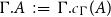 $\Gamma .A\;:=\;\Gamma .\mathcal{c}_{\Gamma }(A)$
. In order to emphasize the difference, we use the superscripts
$\Gamma .A\;:=\;\Gamma .\mathcal{c}_{\Gamma }(A)$
. In order to emphasize the difference, we use the superscripts
 $\_^e,\_^f$
, and write
$\_^e,\_^f$
, and write
 $\texttt {Ty}^e,\texttt {Tm}^e$
for the original CwF structure, and write
$\texttt {Ty}^e,\texttt {Tm}^e$
for the original CwF structure, and write
 $\texttt {Ty}^f,\texttt {Tm}^f$
for the one obtained by the coercion transformation. Unsurprisingly, this choice is intentional to be consistent with the first section. The original CwF will model the “exo” level of 2LTT, while the other models the usual “HoTT” level of 2LTT.
$\texttt {Ty}^f,\texttt {Tm}^f$
for the one obtained by the coercion transformation. Unsurprisingly, this choice is intentional to be consistent with the first section. The original CwF will model the “exo” level of 2LTT, while the other models the usual “HoTT” level of 2LTT.
Example 3.8.
Recall
 $\widehat {\texttt {Ty}}$
denotes the presheaf CwF structure. The simplicial set presheaf
$\widehat {\texttt {Ty}}$
denotes the presheaf CwF structure. The simplicial set presheaf
 $\mathsf{SSet}$
originally had a presheaf CwF structure. Recall that
$\mathsf{SSet}$
originally had a presheaf CwF structure. Recall that
 \begin{equation*}\texttt {Ty}(P)\;:=\;\{A : \widehat {\texttt {Ty}}(P) \mid p_A : P.A \rightarrow P \text{ is a Kan fibration}\}\end{equation*}
gives another type functor. Taking
 $\texttt {Ty}^f=\texttt {Ty}$
and
$\texttt {Ty}^f=\texttt {Ty}$
and
 $\mathcal{c} : \texttt {Ty}^f \rightarrow \widehat {\texttt {Ty}}$
as the inclusion, we obtain
$\mathcal{c} : \texttt {Ty}^f \rightarrow \widehat {\texttt {Ty}}$
as the inclusion, we obtain
 $\mathsf{SSet}$
as a two-level Cwf.
$\mathsf{SSet}$
as a two-level Cwf.
In a similar vein to how we can build a presheaf CwF from any arbitrary (small) category when the category itself is a CwF, we can proceed to construct a two-level CwF. This particular construction, which we refer to as the presheaf two-level CwF, will serve as our primary focus and model of interest.
Definition 3.9.
Let
 $\mathcal{C}$
be a (small) category with CwF structure
$\mathcal{C}$
be a (small) category with CwF structure
 $\texttt {Ty}$
,
$\texttt {Ty}$
,
 $\texttt {Tm}$
. There is a two-level CwF structure on
$\texttt {Tm}$
. There is a two-level CwF structure on
 $\widehat {\mathcal{C}}$
called presheaf two-level CwF, denoted by
$\widehat {\mathcal{C}}$
called presheaf two-level CwF, denoted by
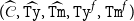 $(\widehat {\mathcal{C}},\widehat {\texttt {Ty}}, \widehat {\texttt {Tm}},\texttt {Ty}^f,\texttt {Tm}^f)$
defined as follows:
$(\widehat {\mathcal{C}},\widehat {\texttt {Ty}}, \widehat {\texttt {Tm}},\texttt {Ty}^f,\texttt {Tm}^f)$
defined as follows:
-
•
$(\widehat {\mathcal{C}},\widehat {\texttt {Ty}}, \widehat {\texttt {Tm}})$
is the presheaf CwF,
-
• given
$P$
in
$\widehat {\mathcal{C}}$
, the type functor
$\texttt {Ty}^f$
is given by
$\texttt {Ty}^f(P)\;:=\;\widehat {\mathcal{C}}(P,\texttt {Ty})$
, and
-
• for
$\Gamma$
in
$\mathcal{C}$
and
$B$
in
$P(\Gamma )$
, we define
$\mathcal{c}_P(A)(\Gamma ,B)\;:=\;\texttt {Tm}(\Gamma ,A_{\Gamma }(B))$
.


As before, given
 $A$
in
$A$
in
 $\texttt {Ty}^f(P)$
, we define
$\texttt {Ty}^f(P)$
, we define
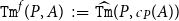 $\texttt {Tm}^f(P,A)\;:=\;\widehat {\texttt {Tm}}(P,\mathcal{c}_P(A))$
.
$\texttt {Tm}^f(P,A)\;:=\;\widehat {\texttt {Tm}}(P,\mathcal{c}_P(A))$
.
Similar to how a type theory can be interpreted within the framework of a category with families, two-level type theories can be interpreted using a two-level category with families. Below, we provide the precise definition for such an interpretation.
Definition 3.10.
A two-level model of a type theory with type formers
 $T^f$
and exo-type formers
$T^f$
and exo-type formers
 $T^e$
is a two-level CwF on a category
$T^e$
is a two-level CwF on a category
 $\mathcal{C}$
such that
$\mathcal{C}$
such that
-
• the structure
$\texttt {Ty}^f,\texttt {Tm}^f$
is a model of type theory with
$T^f$
, -
• the structure
$\texttt {Ty}^e,\texttt {Tm}^e$
is a model of type theory with
$T^e$
.


Remark 3.11. From now on, when we say a two-level model with enough type formers or a model of 2LTT, we mean the two-level model with
 $T^f$
and
$T^f$
and
 $T^e$
where the collections are the types and exo-types given at the beginning of the previous section.
$T^e$
where the collections are the types and exo-types given at the beginning of the previous section.
Our only assumption concerning the coercion morphism
 $\texttt {Ty}^f \rightarrow \texttt {Ty}^e$
is that it is a natural transformation. However, in the context of a two-level model with enough type formers, we have the semantic counterpart of Theorem2.4. This theorem furnishes nice inversion rules from types to exo-types, and its proof heavily relies on the preservation of context extension and the elimination rules associated with the type formers (Annenkov et al., Reference Annenkov, Capriotti, Kraus and Sattler2023).
$\texttt {Ty}^f \rightarrow \texttt {Ty}^e$
is that it is a natural transformation. However, in the context of a two-level model with enough type formers, we have the semantic counterpart of Theorem2.4. This theorem furnishes nice inversion rules from types to exo-types, and its proof heavily relies on the preservation of context extension and the elimination rules associated with the type formers (Annenkov et al., Reference Annenkov, Capriotti, Kraus and Sattler2023).
3.2 Models with cofibrant exo-nat
With the foundational knowledge established thus far, we are now equipped to delve into the discussion of potential models of 2LTT that satisfy the condition of having a cofibrant exo-nat. However, before proceeding to where this discussion takes place, let us first provide the semantic definition of “cofibrancy” for an exo-type.
Definition 3.12.
Let
 $(\mathcal{C}, \texttt {Ty}^e, \texttt {Tm}^e, \texttt {Ty}^f, \texttt {Tm}^f)$
be a model of 2LTT with conversion
$(\mathcal{C}, \texttt {Ty}^e, \texttt {Tm}^e, \texttt {Ty}^f, \texttt {Tm}^f)$
be a model of 2LTT with conversion
 $\mathcal{c}:\texttt {Ty}^f\rightarrow \texttt {Ty}^e$
. We say an exo-type
$\mathcal{c}:\texttt {Ty}^f\rightarrow \texttt {Ty}^e$
. We say an exo-type
 $A:\texttt {Ty}^e(\Gamma )$
is cofibrant if for any
$A:\texttt {Ty}^e(\Gamma )$
is cofibrant if for any
 $\Delta : \mathcal{C}$
and
$\Delta : \mathcal{C}$
and
 $\sigma : \Delta \rightarrow \Gamma$
-
(1) there is a map, natural in
$\Delta$
,such that for any
\begin{equation*}\Theta ^{\texttt {Ty}}_{\Delta }:\texttt {Ty}^f(\Delta .A[\sigma ])\rightarrow \texttt {Ty}^f(\Delta ) \end{equation*}
$Y:\texttt {Ty}^f(\Delta .A[\sigma ])$
we have the following isomorphism natural in
$\Delta$
;
\begin{equation*}\mathcal{c}_{\Delta }(\Theta ^{\texttt {Ty}}_{\Delta }(Y))\cong {\prod }^e(A,\mathcal{c}_{\Delta .A[\sigma ]}(Y)), \end{equation*}
-
(2) and there is a map, natural in
$\Delta$
,In other words, if
\begin{equation*}\Theta ^{\texttt {Tm}}_{\Delta }:\texttt {Tm}^f\left (\Delta .A[\sigma ],{\mathsf{isContr}}(Y)\right ) \rightarrow \texttt {Tm}^f\left (\Delta ,{\mathsf{isContr}}(\Theta _{\Delta }^{\texttt {Ty}}(Y))\right ).\end{equation*}
$Y$
is contractible, then so is
$\Theta ^{\texttt {Ty}}_{\Gamma }(Y)$
.


Remark 3.13. This does not represent a direct translation of the internal definition; rather, it can be seen as a universe-free adaptation of it. In Definition 2.11, the quantification is over specific types within a particular universe. Externally, we can express it in terms of all types. Consequently, the external version holds slightly more strength.
The naturality conditions give the following: In Figure 2, all vertical arrows are context substitutions. When the commutative sides are appropriately composed, the top and bottom isomorphisms are equal, which can be expressed as the cube “commuting.” In Figure 3, the vertical arrows are context substitutions, and the square is commutative.
Naturality condition for
 $\Theta ^{\texttt {Ty}}$
, where
$\Theta ^{\texttt {Ty}}$
, where
 $\sigma :\Delta \rightarrow \Gamma$
and
$\sigma :\Delta \rightarrow \Gamma$
and
 $\tau : \Upsilon \rightarrow \Delta$
in
$\tau : \Upsilon \rightarrow \Delta$
in
 $\mathcal{C}$
.
$\mathcal{C}$
.

Naturality condition for
 $\Theta ^{\texttt {Tm}}$
, where
$\Theta ^{\texttt {Tm}}$
, where
 $\sigma :\Delta \rightarrow \Gamma$
and
$\sigma :\Delta \rightarrow \Gamma$
and
 $\tau : \Upsilon \rightarrow \Delta$
in
$\tau : \Upsilon \rightarrow \Delta$
in
 $\mathcal{C}$
.
$\mathcal{C}$
.

In the following definition, recall that all products exist in the category of sets.
Definition 3.14.
Let
 $(\mathcal{C}, \texttt {Ty}, \texttt {Tm})$
be a CwF with enough type formers. We say
$(\mathcal{C}, \texttt {Ty}, \texttt {Tm})$
be a CwF with enough type formers. We say
 $\mathcal{C}$
has exo-nat products if there is a map
$\mathcal{C}$
has exo-nat products if there is a map
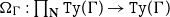 $\Omega _{\Gamma }:\prod _{\mathbf{N}}\texttt {Ty}(\Gamma )\rightarrow \texttt {Ty}(\Gamma )$
, where
$\Omega _{\Gamma }:\prod _{\mathbf{N}}\texttt {Ty}(\Gamma )\rightarrow \texttt {Ty}(\Gamma )$
, where
 $\mathbf{N}$
is the external natural numbers, such that for any
$\mathbf{N}$
is the external natural numbers, such that for any
 $Y : \prod _{\mathbf{N}}\texttt {Ty}(\Gamma )$
we have
$Y : \prod _{\mathbf{N}}\texttt {Ty}(\Gamma )$
we have
-
(1) the set
$\texttt {Tm}(\Gamma , \Omega _{\Gamma }(Y))$
is isomorphic to the categorical product of the sets
$\texttt {Tm}(\Gamma , Y_a)$
for each
$a:\mathbf{N}$
, namely, we have
-
(2) if
$d,c : \prod _{a:\mathbf{N}} \texttt {Tm}(\Gamma ,Y_a)$
are such that there is a term in the type
$\mathsf{Id}(d_a,c_a)$
as being terms of
$Y_a:\texttt {Ty}(\Gamma )$
, then there is a term in the type
$\mathsf{Id}(\psi (d),\psi (c))$
as being terms of
$\Omega _{\Gamma }(Y)$
,


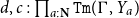


and all these are natural in
 $\Gamma$
.
$\Gamma$
.
In simpler terms, the first requirement stated in Definition 3.14 ensures that
 $\prod ^e_{a:\mathbb{N}^e} Y(a)$
has a fibrant match, while the second requirement ensures that the
$\prod ^e_{a:\mathbb{N}^e} Y(a)$
has a fibrant match, while the second requirement ensures that the
 $\mathsf{funext}$
condition for cofibrant exo-types holds. Therefore, we have the semantic counterpart of Proposition 2.12:
$\mathsf{funext}$
condition for cofibrant exo-types holds. Therefore, we have the semantic counterpart of Proposition 2.12:
Lemma 3.15.
Let
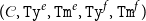 $(\mathcal{C},\texttt {Ty}^e,\texttt {Tm}^e,\texttt {Ty}^f,\texttt {Tm}^f)$
be a two-level CwF model of 2LTT equipped with the coercion
$(\mathcal{C},\texttt {Ty}^e,\texttt {Tm}^e,\texttt {Ty}^f,\texttt {Tm}^f)$
be a two-level CwF model of 2LTT equipped with the coercion
 $\mathcal{c}:\texttt {Ty}^f\!\to \!\texttt {Ty}^e$
. Fix an exo-type
$\mathcal{c}:\texttt {Ty}^f\!\to \!\texttt {Ty}^e$
. Fix an exo-type
 $A:\texttt {Ty}^e(\Gamma )$
and a context morphism
$A:\texttt {Ty}^e(\Gamma )$
and a context morphism
 $\sigma :\Delta \to \Gamma$
. Assume that condition (1) of Definition 3.12 holds, namely we have a natural transformation
$\sigma :\Delta \to \Gamma$
. Assume that condition (1) of Definition 3.12 holds, namely we have a natural transformation
 \begin{equation*} \Theta ^{\texttt {Ty}}_{\Delta }\;:\; \texttt {Ty}^f(\Delta .A[\sigma ])\;\longrightarrow \;\texttt {Ty}^f(\Delta ) \quad \text{ with } \quad \mathcal{c}_{\Delta }\!\bigl (\Theta ^{\texttt {Ty}}_{\Delta }(Y)\bigr ) \;\cong \; {\prod \nolimits }^{e}\!(A,\mathcal{c}_{\Delta .A[\sigma ]}(Y)). \end{equation*}
Then following statements are equivalent: For every
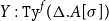 $Y:\texttt {Ty}^f(\Delta .A[\sigma ])$
,
$Y:\texttt {Ty}^f(\Delta .A[\sigma ])$
,
-
i. there is a map, natural in
$\Delta$
,
\begin{equation*}\Theta ^{\texttt {Tm}}_{\Delta }:\texttt {Tm}^f\left (\Delta .A[\sigma ],{\mathsf{isContr}}(Y)\right ) \rightarrow \texttt {Tm}^f\left (\Delta ,{\mathsf{isContr}}(\Theta _{\Delta }^{\texttt {Ty}}(Y))\right ).\end{equation*}
-
ii. if
$d,c:\prod _{a:A}\texttt {Tm}^f(\Delta ,Y[a])$
are such that the terms
$\texttt {Tm}^f\bigl (\Delta ,\mathsf{Id}_{Y[a]}(d_a,c_a)\bigr )$
exist for all
$a:A$
then the terms
also exists, where
\begin{equation*} \texttt {Tm}^f\Bigl (\Delta ,\; \mathsf{Id}_{\Theta ^{\texttt {Ty}}_{\Delta }(Y)} \bigl (\psi (d),\psi (c)\bigr ) \Bigr ) \end{equation*}
$\psi :\prod _{a:A}\texttt {Tm}^f(\Delta ,Y[a])\to \texttt {Tm}^f(\Delta ,\Theta ^{\texttt {Ty}}_{\Delta }(Y))$
is the inverse in the isomorphism of condition (1).


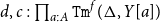
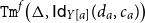


Proof.
Instantiate Proposition 2.12 with the context
 $\Delta .A[\sigma ]$
and the family
$\Delta .A[\sigma ]$
and the family
 $Y:\texttt {Ty}^f(\Delta .A[\sigma ])$
. Soundness of the 2LTT interpretation implies that the internal equivalence proved in 2.12 holds in every model, yielding the desired equivalence between (i) and (ii).
$Y:\texttt {Ty}^f(\Delta .A[\sigma ])$
. Soundness of the 2LTT interpretation implies that the internal equivalence proved in 2.12 holds in every model, yielding the desired equivalence between (i) and (ii).
We now give a canonical instance of a CWF with exo-nat products.
Example 3.16.
Let
 $\mathcal{C}$
be a simplicial model category (Hovey, Reference Hovey1999). Write
$\mathcal{C}$
be a simplicial model category (Hovey, Reference Hovey1999). Write
 ${\mathcal{C}}/{\Gamma }$
for the slice over a context
${\mathcal{C}}/{\Gamma }$
for the slice over a context
 $\Gamma \in \mathcal{C}$
. Define
$\Gamma \in \mathcal{C}$
. Define
 $\texttt {Ty}(\Gamma )$
as the set of fibrations over
$\texttt {Ty}(\Gamma )$
as the set of fibrations over
 $\Gamma$
(with suitable coherence conditions (Lumsdaine and Warren, Reference Lumsdaine and Warren2015)). Define for
$\Gamma$
(with suitable coherence conditions (Lumsdaine and Warren, Reference Lumsdaine and Warren2015)). Define for
 $A: \texttt {Ty}(\Gamma )$
the set
$A: \texttt {Ty}(\Gamma )$
the set
 $\texttt {Tm}(\Gamma ,P)$
as the hom-set
$\texttt {Tm}(\Gamma ,P)$
as the hom-set
 ${\mathcal{C}}/{\Gamma }[\Gamma , \Gamma .A ]$
.
${\mathcal{C}}/{\Gamma }[\Gamma , \Gamma .A ]$
.
Fibrations are closed under pullback in any model category, and products are pullbacks of the projections. Hence the product of a countable family of fibrations is again a fibration. Given a family
 $Y\colon \mathbf N\to \texttt {Ty}(\Gamma )$
, set
$Y\colon \mathbf N\to \texttt {Ty}(\Gamma )$
, set
 \begin{equation*} \Omega _\Gamma (Y)\;\;:=\;\;\prod _{n:\mathbf N} Y_n \;\in \;\texttt {Ty}(\Gamma ). \end{equation*}
Because sections are morphisms in the slice, the universal property of products induces a canonical natural isomorphism
 \begin{equation*} \texttt {Tm} \bigl (\Gamma ,\Omega _\Gamma (Y)\bigr ) \;\cong \; \prod _{n:\mathbf N}\texttt {Tm} \bigl (\Gamma ,Y_n\bigr ), \end{equation*}
verifying clause (1) of Definition 3.14 .
Since
 $\mathcal{C}$
is simplicial, each slice
$\mathcal{C}$
is simplicial, each slice
 $\mathcal{C}/\Gamma$
is tensored and cotensored with simplicial sets, giving an adjunction
$\mathcal{C}/\Gamma$
is tensored and cotensored with simplicial sets, giving an adjunction
 \begin{equation} (\!-\!)\!\otimes \!\Delta [1]\;\dashv \;(\!-\!)^{\Delta [1]} \;:\;\mathcal{C}/\Gamma \;\longrightarrow \;\mathcal{C}/\Gamma . \end{equation}
For a fibration
 $p:A\rightarrow \Gamma$
define the identification object
$p:A\rightarrow \Gamma$
define the identification object
 \begin{equation*} \mathsf{Id}_A\;\;:=\;\;A^{\Delta [1]} . \end{equation*}
Because
 $(\!-\!)^{\!\Delta [1]}$
is the right adjoint in (6), it preserves limits, yielding the natural isomorphism
$(\!-\!)^{\!\Delta [1]}$
is the right adjoint in (6), it preserves limits, yielding the natural isomorphism
 \begin{equation} \Bigl (\prod _{n:\mathbf N} Y_n\Bigr )^{\!\Delta [1]} \;\cong \; \prod _{n:\mathbf N} Y_n^{\Delta [1]} . \end{equation}
Let
 \begin{equation*} d,c\;:\;\prod _{n:\mathbf N}\texttt {Tm}(\Gamma ,Y_n), \qquad h_n\;:\;\texttt {Tm}\bigl (\Gamma ,\mathsf{Id}_{Y_n}(d_n,c_n)\bigr ). \end{equation*}
Transport the tuple
 $(h_n)_{n:\mathbf N}$
across (7); via the slice/section identification, this yields a single
$(h_n)_{n:\mathbf N}$
across (7); via the slice/section identification, this yields a single
 \begin{equation*} h\;:\;\texttt {Tm} \bigl (\Gamma ,\mathsf{Id}_{\Omega _\Gamma (Y)}(d,c)\bigr ). \end{equation*}
Restricting
 $h$
along the projections recovers each
$h$
along the projections recovers each
 $h_n$
, so the correspondence is bijective. Because (7) is natural in
$h_n$
, so the correspondence is bijective. Because (7) is natural in
 $\Gamma$
(it is the mate of (6)), clause (2) of Definition 3.14 is satisfied naturally.
$\Gamma$
(it is the mate of (6)), clause (2) of Definition 3.14 is satisfied naturally.
In Theorem3.17, we provide a class of two-level CwFs that satisfy the axiom that
 $\mathbb{N}^e$
is a cofibrant exo-type.
$\mathbb{N}^e$
is a cofibrant exo-type.
Theorem 3.17.
If
 $(\mathcal{C}, \texttt {Ty}, \texttt {Tm})$
is CwF (with sufficient type formers) has exo-nat products, the corresponding two-level CwF obtained by Definition 3.9 satisfies the axiom that
$(\mathcal{C}, \texttt {Ty}, \texttt {Tm})$
is CwF (with sufficient type formers) has exo-nat products, the corresponding two-level CwF obtained by Definition 3.9 satisfies the axiom that
 $\mathbb{N}^e$
is a cofibrant exo-type.
$\mathbb{N}^e$
is a cofibrant exo-type.
Proof.
Recall that
 $\mathbb{N}^e : \widehat {\texttt {Ty}}(1_{\widehat {\mathcal{C}}})$
. For any
$\mathbb{N}^e : \widehat {\texttt {Ty}}(1_{\widehat {\mathcal{C}}})$
. For any
 $P :\widehat {\mathcal{C}}$
, the context morphism
$P :\widehat {\mathcal{C}}$
, the context morphism
 $\sigma : P \rightarrow 1_{\widehat {\mathcal{C}}}$
is unique, so we omit substitutions over such morphisms and write
$\sigma : P \rightarrow 1_{\widehat {\mathcal{C}}}$
is unique, so we omit substitutions over such morphisms and write
 $P.\mathbb{N}^e$
instead of
$P.\mathbb{N}^e$
instead of
 $P.\mathbb{N}^e[\sigma ]$
.
$P.\mathbb{N}^e[\sigma ]$
.
First, we define the map
 $\Theta ^{\texttt {Ty}}_{P}:\texttt {Ty}^f(P.\mathbb{N}^e)\rightarrow \texttt {Ty}^f(P)$
. For any
$\Theta ^{\texttt {Ty}}_{P}:\texttt {Ty}^f(P.\mathbb{N}^e)\rightarrow \texttt {Ty}^f(P)$
. For any
 $Y : \texttt {Ty}^f(P.\mathbb{N}^e) = \widehat {\mathcal{C}}(P.\mathbb{N}^e, \texttt {Ty})$
, we need
$Y : \texttt {Ty}^f(P.\mathbb{N}^e) = \widehat {\mathcal{C}}(P.\mathbb{N}^e, \texttt {Ty})$
, we need
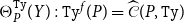 $\Theta ^{\texttt {Ty}}_{P}(Y): \texttt {Ty}^f(P)=\widehat {\mathcal{C}}(P, \texttt {Ty})$
. We denote
$\Theta ^{\texttt {Ty}}_{P}(Y): \texttt {Ty}^f(P)=\widehat {\mathcal{C}}(P, \texttt {Ty})$
. We denote
 $\Theta ^{\texttt {Ty}}_{P}(Y)$
by
$\Theta ^{\texttt {Ty}}_{P}(Y)$
by
 $\tilde {Y}$
for easier reading. Now, for
$\tilde {Y}$
for easier reading. Now, for
 $\Gamma : \mathcal{C}$
and
$\Gamma : \mathcal{C}$
and
 $x : P_{\Gamma }$
, we define
$x : P_{\Gamma }$
, we define
 \begin{equation*}\tilde {Y}_{\Gamma }(x)\;:=\; \Omega _{\Gamma }\left ( (Y_{\Gamma }(x,n))_n\right )\end{equation*}
where the map
 $\Omega _{\Gamma } : \prod _{\mathbf{N}} \texttt {Ty}(\Gamma ) \rightarrow \texttt {Ty}(\Gamma )$
is obtained by the assumption of having exo-nat products, Definition 3.14. The definition makes sense since we have
$\Omega _{\Gamma } : \prod _{\mathbf{N}} \texttt {Ty}(\Gamma ) \rightarrow \texttt {Ty}(\Gamma )$
is obtained by the assumption of having exo-nat products, Definition 3.14. The definition makes sense since we have
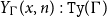 $Y_{\Gamma }(x,n) : \texttt {Ty}(\Gamma )$
. We want to show
$Y_{\Gamma }(x,n) : \texttt {Ty}(\Gamma )$
. We want to show
 \begin{equation*} \mathcal{c}_P(\tilde {Y}) \cong {\prod }^e(\mathbb{N}^e, \mathcal{c}_{P.\mathbb{N}^e}(Y)).\end{equation*}
Both are elements in
 $\widehat {\texttt {Ty}}(P)$
, namely, presheaves over
$\widehat {\texttt {Ty}}(P)$
, namely, presheaves over
 $\int P$
. Thus, it is enough to define a natural transformation
$\int P$
. Thus, it is enough to define a natural transformation
 $G: \mathcal{c}_P(\tilde {Y}) \rightarrow \prod ^e(\mathbb{N}^e, \mathcal{c}_{P.\mathbb{N}^e}(Y))$
such that for any
$G: \mathcal{c}_P(\tilde {Y}) \rightarrow \prod ^e(\mathbb{N}^e, \mathcal{c}_{P.\mathbb{N}^e}(Y))$
such that for any
 $\Gamma : \mathcal{C}$
and
$\Gamma : \mathcal{C}$
and
 $x : P_{\Gamma }$
, the map
$x : P_{\Gamma }$
, the map
 \begin{equation*}G_{\Gamma ,x} : \mathcal{c}_P(\tilde {Y})(\Gamma ,x) \rightarrow {\prod }^e(\mathbb{N}^e, \mathcal{c}_{P.\mathbb{N}^e}(Y)) (\Gamma ,x)\end{equation*}
is an isomorphism of sets, namely, a bijection. If we elaborate on these a little further, we obtain the following. By definition,
 $\mathcal{c}_P(\tilde {Y})(\Gamma ,x)=\texttt {Tm}(\Gamma , \tilde {Y}_{\Gamma }(x))$
. Also,
$\mathcal{c}_P(\tilde {Y})(\Gamma ,x)=\texttt {Tm}(\Gamma , \tilde {Y}_{\Gamma }(x))$
. Also,
 ${\prod }^e(\mathbb{N}^e, \mathcal{c}_{P.\mathbb{N}^e}(Y)) (\Gamma ,x)$
consists of the elements
${\prod }^e(\mathbb{N}^e, \mathcal{c}_{P.\mathbb{N}^e}(Y)) (\Gamma ,x)$
consists of the elements
 \begin{equation*}f : \prod _{\substack {\Delta : \mathcal{C} \\ \sigma : \Delta \rightarrow \Gamma \\ n : \mathbb{N}^e (\Delta , x[\sigma ])}} \mathcal{c}_{P.\mathbb{N}^e}(Y)(\Delta , x[\sigma ], n)(=\texttt {Tm}(\Delta , Y_{\Delta }(x[\sigma ],n)))\end{equation*}
such that if
 $\Upsilon : \mathcal{C}$
and
$\Upsilon : \mathcal{C}$
and
 $\tau : \Upsilon \rightarrow \Delta$
, then
$\tau : \Upsilon \rightarrow \Delta$
, then
 $f(\Delta , \sigma , n)[\tau ]=f(\Upsilon , \sigma \circ \tau , n[\tau ])$
. By the definition of
$f(\Delta , \sigma , n)[\tau ]=f(\Upsilon , \sigma \circ \tau , n[\tau ])$
. By the definition of
 $\mathbb{N}^e$
, we have
$\mathbb{N}^e$
, we have
 $\mathbb{N}^e(\Delta ,x[\sigma ])=\mathbf{N}$
, external natural number set, and having exo-nat products provides us
$\mathbb{N}^e(\Delta ,x[\sigma ])=\mathbf{N}$
, external natural number set, and having exo-nat products provides us
 \begin{equation*}\prod _{n :\mathbf{N}} \texttt {Tm}(\Delta , Y_{\Delta }(x[\sigma ],n)) \cong \texttt {Tm}(\Delta , \tilde {Y}(x[\sigma ])).\end{equation*}
Thus, the range of
 $G_{\Gamma ,x}$
can be written as
$G_{\Gamma ,x}$
can be written as
 \begin{equation*}f : \prod _{\substack {\Delta : \mathcal{C} \\ \sigma : \Delta \rightarrow \Gamma }} \texttt {Tm}(\Delta , \tilde {Y}_{\Delta }(x[\sigma ]))\end{equation*}
such that if
 $\Upsilon : \mathcal{C}$
and
$\Upsilon : \mathcal{C}$
and
 $\tau : \Upsilon \rightarrow \Delta$
, then
$\tau : \Upsilon \rightarrow \Delta$
, then
 $f(\Delta , \sigma )[\tau ]=f(\Upsilon , \sigma \circ \tau )$
. This elaboration allows us to easily perceive that this function is a bijection because it is a standard application of the Yoneda Lemma. The naturality condition of this operation is also easily satisfied because the substitution is functorial. Thus, we have confirmed the first stage of our claim.
$f(\Delta , \sigma )[\tau ]=f(\Upsilon , \sigma \circ \tau )$
. This elaboration allows us to easily perceive that this function is a bijection because it is a standard application of the Yoneda Lemma. The naturality condition of this operation is also easily satisfied because the substitution is functorial. Thus, we have confirmed the first stage of our claim.
By Lemma 3.15 the contractibility requirement is already satisfied; therefore,
 $\mathbb{N}^e$
is a cofibrant exo-type in the presheaf two-level CwF.
$\mathbb{N}^e$
is a cofibrant exo-type in the presheaf two-level CwF.
Remark 3.18. The proof of Theorem 3.17 actually factors through a more general statement suggested by the referee:
Let
 $I$
be an external set. If
$I$
be an external set. If
 $(\mathcal{C}, \texttt {Ty}, \texttt {Tm})$
is a CwF (with sufficient type formers) where
$(\mathcal{C}, \texttt {Ty}, \texttt {Tm})$
is a CwF (with sufficient type formers) where
 $I$
-indexed copower of 1 exists, then it is a cofibrant exo-type in the corresponding two-level CwF obtained by Definition 3.9.
$I$
-indexed copower of 1 exists, then it is a cofibrant exo-type in the corresponding two-level CwF obtained by Definition 3.9.
Taking
 $I = \mathbb N$
recovers Theorem 3.17. The proof is identical to the one given above, with every occurrence of
$I = \mathbb N$
recovers Theorem 3.17. The proof is identical to the one given above, with every occurrence of
 $\mathbb N$
replaced by the set
$\mathbb N$
replaced by the set
 $I$
; Lemma 3.15 supplies the necessary equivalence between the contractibility and identification formulations along the way. We record only the special case needed here and leave the full statement to the reader.
$I$
; Lemma 3.15 supplies the necessary equivalence between the contractibility and identification formulations along the way. We record only the special case needed here and leave the full statement to the reader.
Remark 3.19. Example 3.16 also enables us to construct a two-level CwF out of the class in the theorem, that satisfies the general result above. Indeed, we can take
 $\texttt {Ty}^e(\Gamma )$
as the set of all morphisms over
$\texttt {Ty}^e(\Gamma )$
as the set of all morphisms over
 $\Gamma$
, and
$\Gamma$
, and
 $\texttt {Tm}^e$
as the same as
$\texttt {Tm}^e$
as the same as
 $\texttt {Tm}$
, and obtain a two-level CwF
$\texttt {Tm}$
, and obtain a two-level CwF
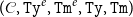 $(\mathcal{C}, \texttt {Ty}^e, \texttt {Tm}^e, \texttt {Ty}, \texttt {Tm})$
with the conversion
$(\mathcal{C}, \texttt {Ty}^e, \texttt {Tm}^e, \texttt {Ty}, \texttt {Tm})$
with the conversion
 $\mathcal{c}:\texttt {Ty}\rightarrow \texttt {Ty}^e$
as being inclusion. It is then enough to take the map
$\mathcal{c}:\texttt {Ty}\rightarrow \texttt {Ty}^e$
as being inclusion. It is then enough to take the map
 $\Theta _{\Gamma }(Y)$
in Definition 3.12 as equal to
$\Theta _{\Gamma }(Y)$
in Definition 3.12 as equal to
 $\prod _{a:I}Y_a$
.
$\prod _{a:I}Y_a$
.
4. Future directions
As previously mentioned, this formalization project aims to move a study about 2LTT (Ahrens et al., Reference Ahrens, North, Shulman and Tsementzis2025) to Agda. In addition to definitions and results here, we also formalized exo-categories and diagram signatures in that study. More will be added in the future.
We also plan to generalize the results about cofibrancy and sharpness. Natural numbers, lists, and binary trees are all inductive types. The general class of such inductive types is called W-types. Similar to the cofibrant exo-nat axiom, we have been studying possible conditions (or axioms) related to W-types to obtain criteria for cofibrant and sharp W-types. Currently, a study on W-types in 2LTT has not been conducted yet; thus, we plan to work on this open problem. We have already considered some special cases like lists and binary trees. We can use their proofs to find a general pattern if possible. That is why we cared about these cases initially.
We have been studying to improve the Agda library. The experimental feature of Agda we used also reveals some bugs; hence, we plan to solve these issues to obtain precise consistency. Furthermore, it is not unreasonable to think that this study will offer new ideas about the concepts specific to 2LTT.
5. Conclusions
We believe that formalized mathematics does not only play the role of determining the correctness of existing results but also offers new perspectives theoretically. In this context, our Agda library project has yielded new findings about 2LTT. While examining the properties of dependent functions using types at different levels on the one hand, we also analyzed the 2LTT versions of various inductive types. To emphasize the validity of our assumptions in a more general context, we provided a broader model framework instead of the known obvious models.
Our work can be considered in two ways, such that initially, the formalization project aimed to provide the validation of some results in another study (Ahrens et al., Reference Ahrens, North, Shulman and Tsementzis2025). As we elaborated on the details of the proofs, we discovered new tools necessary for formalization and thus enriched the theory (2LTT) with these new tools. In this form, the theory has been formalized without requiring any modification. We think that such studies are a good example of the duality between theory and practice.
We can say that we actually benefited from this formalization work while exploring the models of the theory we are dealing with. We can say that models providing a cofibrant exo-nat were found with the help of an equivalent definition of cofibrancy, and this equivalent definition emerged after the Agda project. These and similar formalization works reinforce our thought; we can include the concept of formalized theory in addition to the duo of object theory and meta-theory.
Acknowledgements
We would like to thank Michael Shulman and Nicolai Kraus for many interesting discussions and insightful comments. The work is partially supported by an NSF grant DMS-1902092, the Army Research Office W911NF-20-1-0075, and the Simons Foundation. The work is also based upon work supported by the Air Force Office of Scientific Research under award number FA9550-21-1-0009.
Competing interests
The author declares no competing interests.


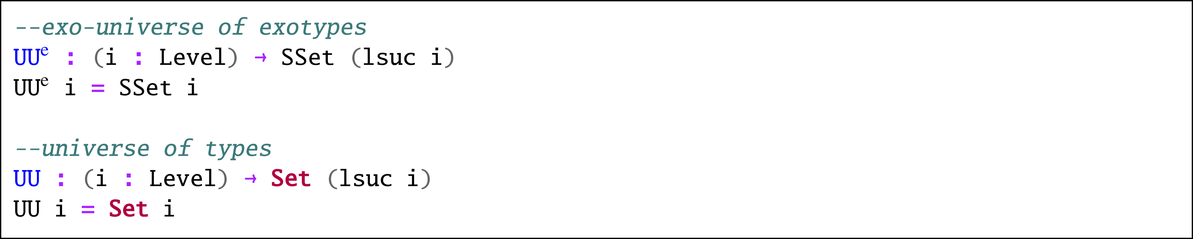


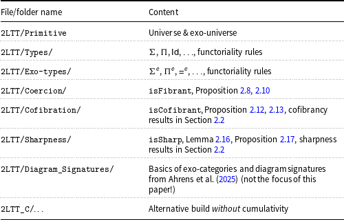
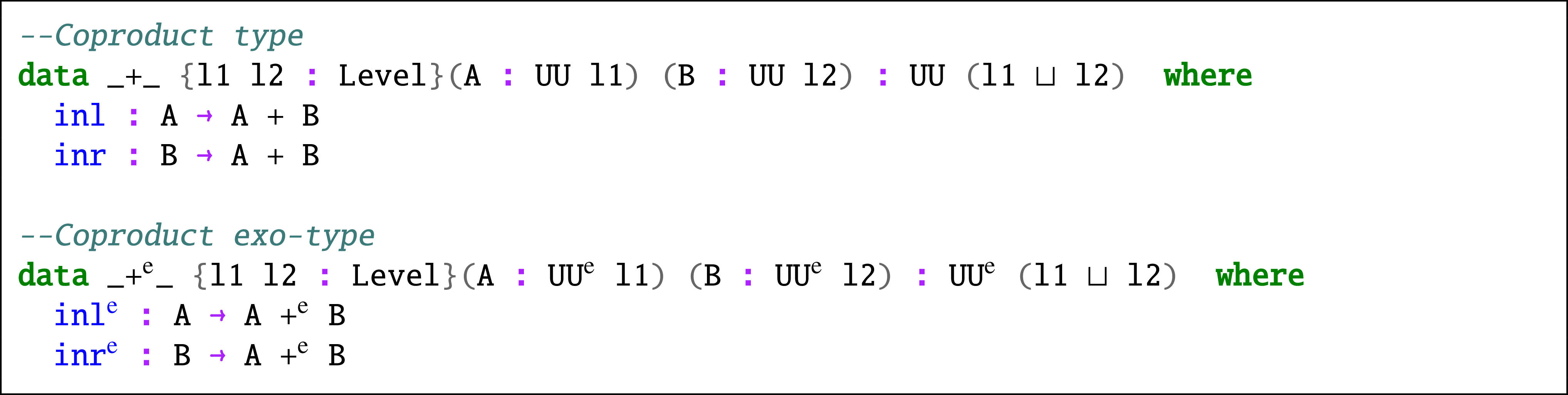

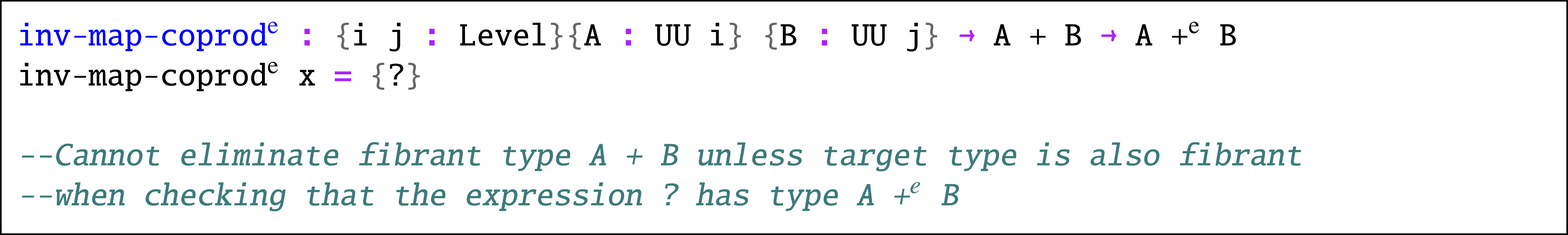

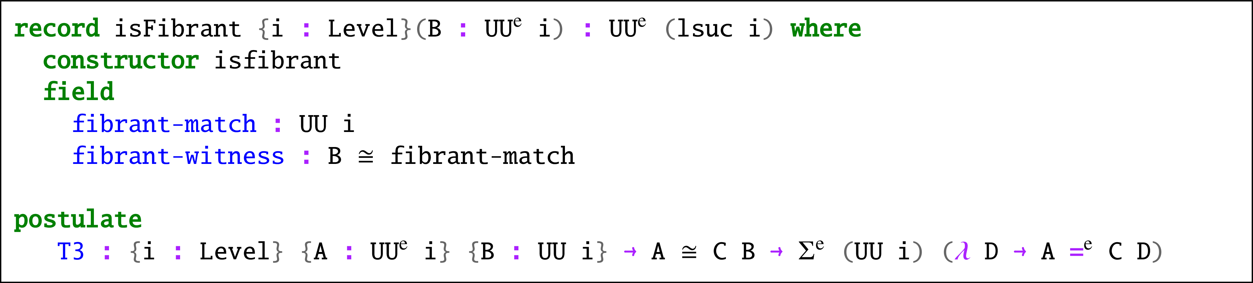
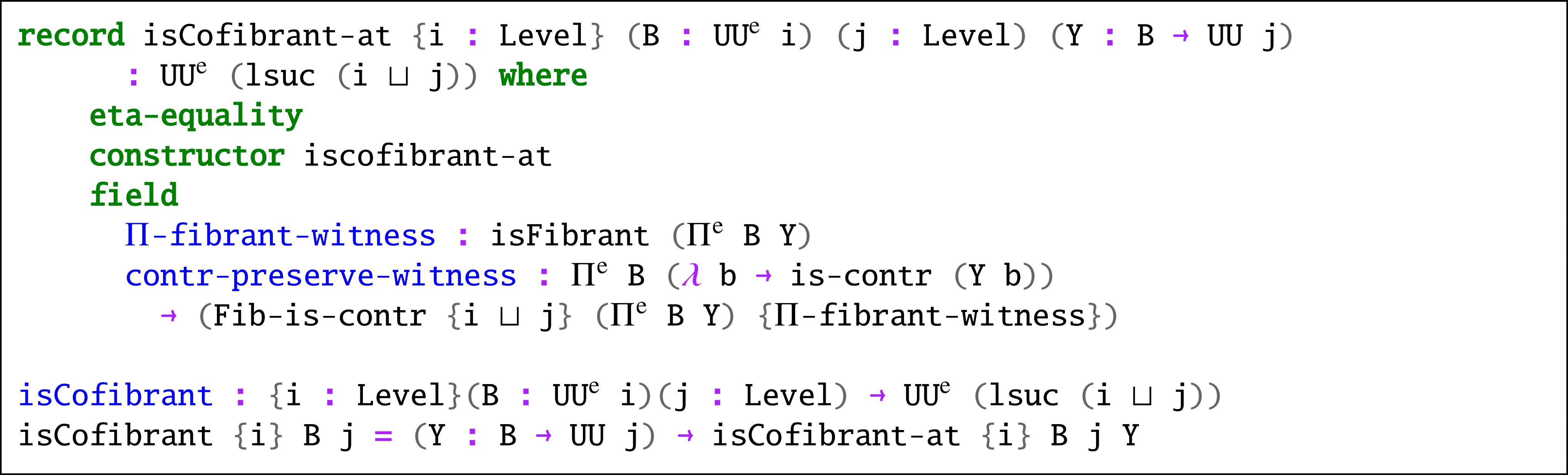
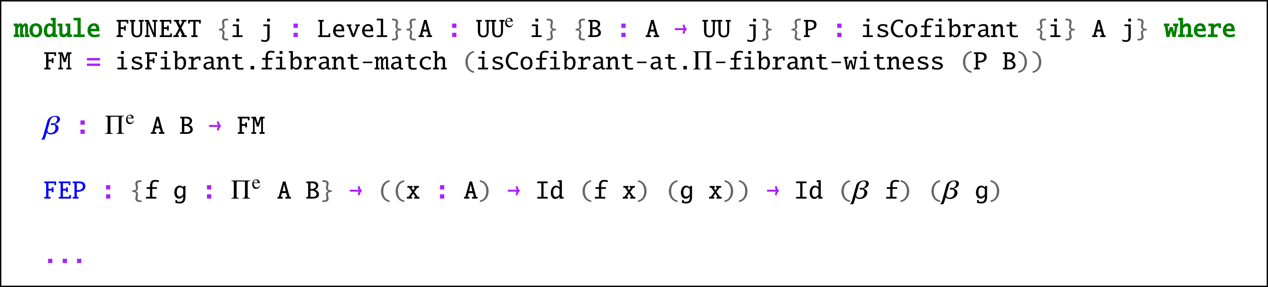
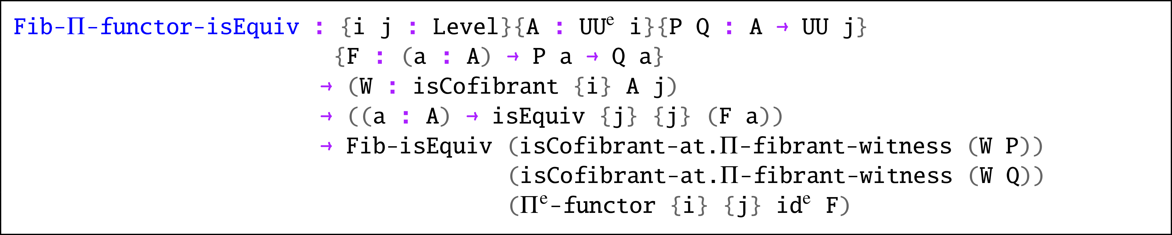


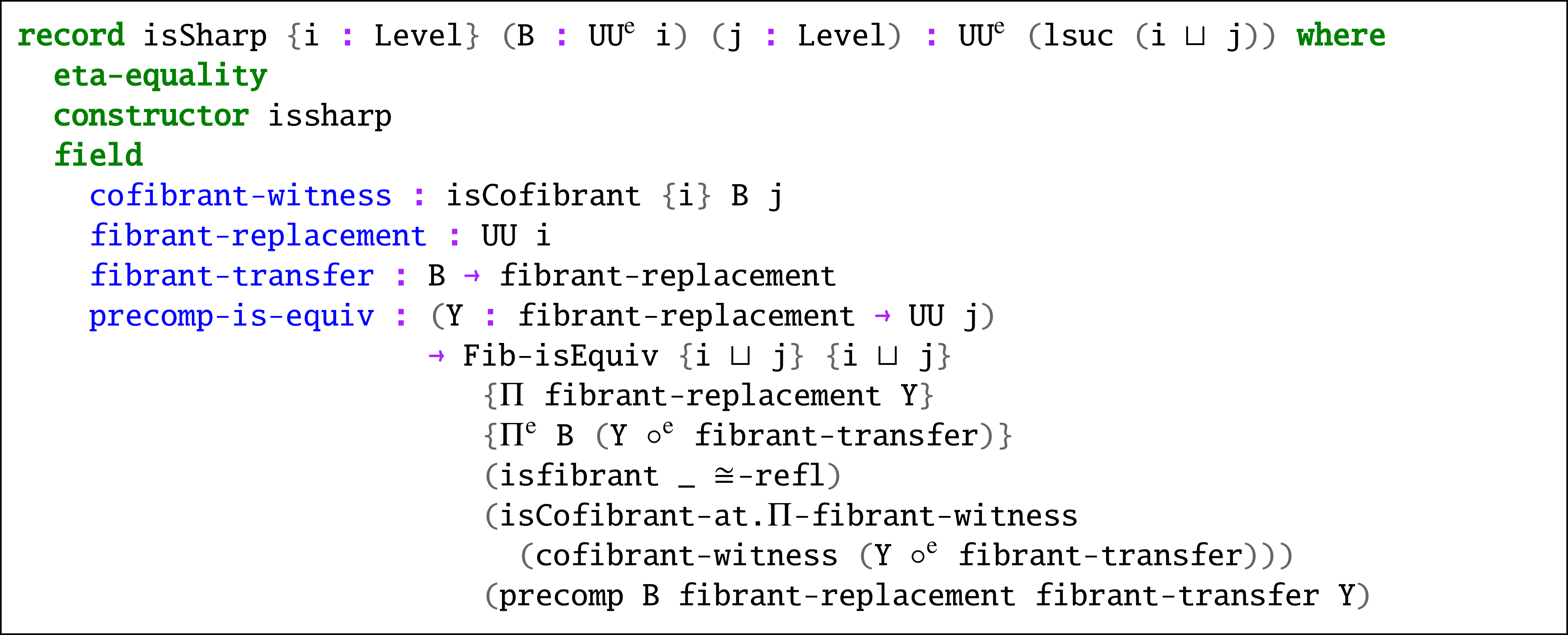
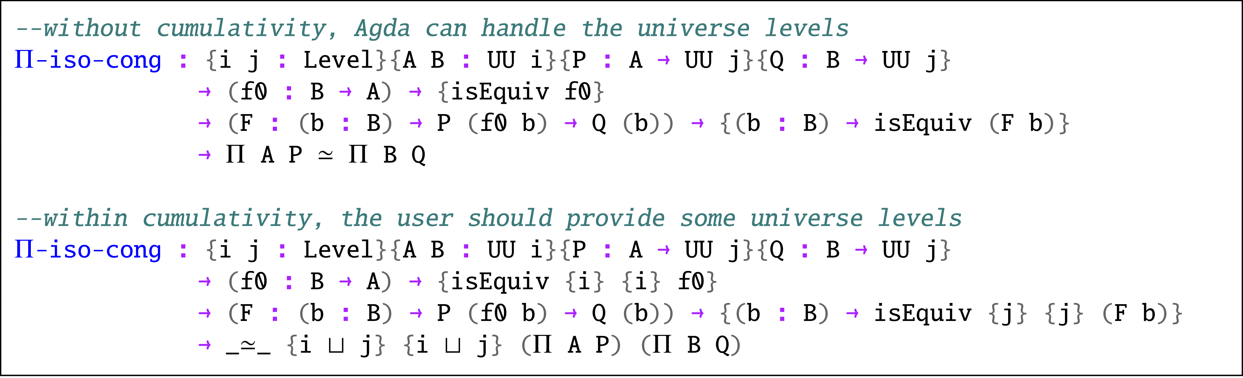


 Open access