


1. Introduction
Fluid flows permeating a porous, thin membrane, have attracted a wide interest in engineering and natural sciences. Biological cells exchange water and nutrients with the environment using protein-based channels on their membranes (Verkman & Mitra Reference Verkman and Mitra2000; Jensen et al. Reference Jensen, Berg-Sørensen, Bruus, Holbrook, Liesche, Schulz, Zwieniecki and Bohr2016). Glass sponges like the Euplectella aspergillum show interesting thin porous skeletons, which ensure their structural stability and allow the feeding of the organisms living inside them. Filtration and separation systems are widely used in the chemical and biomedical industry (Catarino et al. Reference Catarino, Rodrigues, Pinho, Miranda, Minas and Lima2019), water purification technologies (Mohanty & Purkait Reference Mohanty and Purkait2011) and batteries (Lu et al. Reference Lu, Yuan, Zhao, Zhang, Zhang and Li2017; Dai et al. Reference Dai, Xing, Liu, Shi, Deng, Zhao and Li2022). Periodic porous media are adopted in some applications such as regenerators (i.e. porous matrices working as heat exchangers) for refrigerators used in cryogenic applications (Roberts & Desai Reference Roberts and Desai2003) and offer obvious modelling advantages, such as the possibility of retrieving the whole medium properties from the geometric unit cell repeating along the membrane. On the other hand, biological porous membranes can be very irregular (Verkman & Mitra Reference Verkman and Mitra2000) and periodic membranes can become aperiodic due to the loads applied by a fluid flowing across it (Fagbemi et al. Reference Fagbemi, Tahmasebi and Piri2018), erosion or fouling or by the presence of defects in the fabrication process. Non-periodicity is also leveraged to improve the efficiency of filtration devices (Dalwadi et al. Reference Dalwadi, Griffiths and Bruna2015).
The precise and efficient description of flows through porous media plays a key role in many engineering fields. We can classify the modelling of flows across porous media into two families: direct solutions and averaged models. In the first case, we consider the actual geometry of the porous medium and solve the governing equations at all scales of interest. Periodic and aperiodic structures in various flow conditions (Icardi et al. Reference Icardi, Boccardo, Marchisio, Tosco and Sethi2014; Falcucci et al. Reference Falcucci, Amati, Fanelli, Krastev, Polverino, Porfiri and Succi2021) can be studied using this technique with very high accuracy, since the fluid flow solution is accessible up to the smallest scale of interest in time and space. However, these simulations easily become prohibitively computationally expensive, they are rarely scalable and do not adapt well to large parametric studies or optimisation routines. The second family relies on a simplified physical description. We substitute a fictitious homogeneous domain to the actual geometry of the medium characterised by coefficients representing the average properties of the porous structure (Darcy Reference Darcy1856; Dagan Reference Dagan1987). Some authors (Hasimoto Reference Hasimoto1958; Conca Reference Conca1987; Wang Reference Wang1994; Bourgeat et al. Reference Bourgeat, Gipouloux and Marusic-Paloka2001) analytically computed these coefficients in simple, periodic geometries and flow configurations. However, in most cases, they have been empirically found. Non-periodicity of the medium’s microstructure is often introduced in these models using additional correction coefficients (Jensen et al. Reference Jensen, Valente and Stone2014). Such techniques are computationally very cheap compared with direct solutions, but their empiricism limits their predictive power. Averaged models with predictive capabilities are thus an active field of research since they represent a good trade-off between accuracy and computational cost. Multiscale methods such as the volume averaging method (Whitaker Reference Whitaker1999) and homogenisation (Hornung Reference Hornung1997; Mei & Vernescu Reference Mei and Vernescu2010) are at the core of these techniques.
In most homogenisation and volume averaging works, the porous microstructure must show periodicity or exhibit a representative elementary volume(REV), i.e. the minimal geometrical portion of the medium where some properties like permeability are univocally determined in a statistical sense. We refer to the book by Bear & Bachmat (Reference Bear and Bachmat1990) for a formal definition of the REV. In the periodic case, there exists a unit cell containing one (Lācis & Bagheri Reference Lācis and Bagheri2017; Luckins et al. Reference Luckins, Breward, Griffiths and Please2023) or more pores (Shipley & Chapman Reference Shipley and Chapman2010), repeating along the medium geometry. In the REV case, there is no such geometrical repetition along the membrane, but if the microstructure is sufficiently regular, an enclosing volume with the same full membrane statistical properties can be found (Whitaker Reference Whitaker1999). This, however, requires several iterations. For example, Rolland du Roscoat et al. (Reference Rolland du Roscoat, Decain, Thibault, Geindreau and Bloch2007) experimentally determined the extension of such entity in some industrial paper materials using microtomography. Auriault et al. (Reference Auriault, Boutin and Geindreau2009) also pointed out that typically 10 heterogeneities along a direction in the REV are sufficient in several real situations and that the REV reduces to the unit cell for periodic media. Using the REV assumption, Valdés-Parada & Alvarez-Ramírez (Reference Valdés-Parada and Alvarez-Ramírez2011) studied asymmetric diffusion in stratified and fractured porous media and Chernyavsky et al. (Reference Chernyavsky, Leach, Dryden and Jensen2011) studied haemodynamic transport across the villous branches of the human placenta. However, microstructures with slow geometry modifications have also been considered, effectively bridging the gap between the periodic and non-periodic cases. For example, van Noorden (Reference van Noorden2009) studied precipitation and dissolution in a pore of varying volume and Van Noorden & Muntean (Reference Van Noorden and Muntean2011) studied the transport across porous structures with varying diffusivities, while Auton et al. (Reference Auton, Pramanik, Dalwadi, MacMinn and Griffiths2022) studied the transport and sorption in a longitudinally heterogeneous and transversely periodic medium and Alavi et al. (Reference Alavi, Cheikho, Laurent and Ganghoffer2024) introduced a conformal transformation to analyse quasiperiodic porous structures. In many cases, considering spatially varying geometry or flow conditions requires the construction of surrogate models to contain the computational cost. For example, in a previous work (Wittkowski et al. Reference Wittkowski, Ponte, Ledda and Zampogna2024), we adopted a clustering technique (i.e. algorithms used to divide a given dataset into clusters based on a notion of similarity between the elements) to reduce the computational cost of a coupling procedure for inertial flows across thin porous membranes. The problem of coupling the pore-scale and the far-field scale dynamics for reacting flows in bulk porous media has also been investigated by Karimi & Bhattacharya (Reference Karimi and Bhattacharya2024a , Reference Karimi and Bhattacharyab ) using recurrent neural networks.
The works mentioned above were mainly related to bulk porous media, while homogenisation has been proposed as a methodology for the analysis of fluid flows (Zampogna & Gallaire Reference Zampogna and Gallaire2020) and transport of diluted species (Zampogna et al. Reference Zampogna, Ledda and Gallaire2022, Reference Zampogna, Ledda, Wittkowski and Gallaire2023) across thin porous membranes with periodic microstructure. In this framework, the membrane average properties (i.e. the so-called Navier tensors) are the spatially averaged solutions of solvability conditions derived from the equations valid at the pore scale. The Navier tensors encrypt the ability of the fluid to pass across and along the membrane and they are useful in the design of efficient filtration devices (Park et al. Reference Park, Chhatre, Srinivasan, Cohen and McKinley2013). These tensors correspond to and extend the concept of permeability and slip in the case of bulk porous media and impervious rough surfaces, respectively. Ledda et al. (Reference Ledda, Boujo, Camarri, Gallaire and Zampogna2021) embedded homogenisation into an adjoint-based loop for the design of thin, porous membranes, finding optimal aperiodic microstructures maximizing drag for a given macroscopic flow configuration. In their work, the link between the shape of a single solid inclusion and the Navier tensors was mapped for different geometrical parameters using direct solutions of the equations valid at the pore scale. The cost of this mapping scales with the number of pores/inclusions. The interest in a theoretical tool able to efficiently predict how geometrical modifications in the microstructure of a porous thin membrane affect the local average microscopic properties is thus clear. In other words, we search for a mathematical tool able to handle many shape modifications of the microstructure while keeping the computational cost lower than a series of direct evaluations. This is a common situation in many engineering fields, such as in the automotive and aerospace industries, where the shape of vehicles can be optimised to reach a desired objective such as minimizing drag. In many cases, the resulting gradient-based optimisation routines are solved using adjoint equations, see Skinner & Zare-Behtash (Reference Skinner and Zare-Behtash2018) for a review.
Adjoint-based approaches have proven an efficient physics-based technique to forecast how shape changes affect given integral quantities of a flow field in external aerodynamics (Jameson Reference Jameson1988; Jameson et al. Reference Jameson, Martinelli and Pierce1998; Mohammadi & Pironneau Reference Mohammadi and Pironneau2001). In other techniques, such as finite differentiation (Reneaux & Thibert Reference Reneaux and Thibert1985), a set of control points are used to control the shape of objects immersed in a flow. These control points are displaced one by one, and the flow is recomputed for each modified geometry. An approximation of the shape sensitivity is then constructed component by component using finite differences. This simple approach does not require solving additional flow equations, but its cost increases with the number of evaluation points and its precision depends on the discretisation. On the other hand, adjoint methods to compute shape sensitivity are more precise and their cost does not depend on the number of evaluation points on the geometry. However, these techniques require the solution of additional flow equations, the adjoint equations, which allow us to evaluate the gradient mentioned above directly.
In the present paper, we focus on the efficient evaluation of the properties of non-periodic membranes via adjoint-based techniques. To develop our methodology, we consider the model developed in Zampogna & Gallaire (Reference Zampogna and Gallaire2020) for flows past membranes with perfectly periodic pore structure and introduce a technique based on adjoint equations to estimate the gradient of the Navier tensors with respect to an infinitesimal modification of the shape of the solid inclusion, i.e. the shape sensitivity. In § 2 we summarise the model by Zampogna & Gallaire (Reference Zampogna and Gallaire2020) and derive the adjoint problems from the equations governing the system at the pore scale; in § 3 we compare the direct solution of the pore-scale problems with the adjoint-based prediction for a series of shape changes; in § 4 we use the so-developed tools to analyse the fluid flow across non-periodic thin membranes. In § 5, we summarise the main results and discuss future perspectives.
2. Modelling shape changes in porous membranes using first- and second-order adjoint methods
We consider the incompressible flow of a Newtonian fluid of density $\rho$
and viscosity
$\rho$
and viscosity $\mu$
across a thin permeable membrane, depicted in figure 1(
$\mu$
across a thin permeable membrane, depicted in figure 1( $a$
). We denote with
$a$
). We denote with $\hat {x}_i=(\hat {x}_1,\hat {x}_2,\hat {x}_3)$
the (dimensional) global coordinate system, with
$\hat {x}_i=(\hat {x}_1,\hat {x}_2,\hat {x}_3)$
the (dimensional) global coordinate system, with $\hat {u}_i$
and
$\hat {u}_i$
and $\hat {p}$
the dimensional fluid flow velocity and pressure and with
$\hat {p}$
the dimensional fluid flow velocity and pressure and with $\hat {\tau }$
the dimensional time. We also introduce the outward-pointing normal and two tangent vectors to any boundary
$\hat {\tau }$
the dimensional time. We also introduce the outward-pointing normal and two tangent vectors to any boundary $(\hat {\boldsymbol {n}},\hat {\boldsymbol {t}},\hat {\boldsymbol {s}})$
, specified case by case. Locally, on the surface, we can isolate a control volume containing few pores/solid inclusions and identify a dimensional local reference frame
$(\hat {\boldsymbol {n}},\hat {\boldsymbol {t}},\hat {\boldsymbol {s}})$
, specified case by case. Locally, on the surface, we can isolate a control volume containing few pores/solid inclusions and identify a dimensional local reference frame $(\hat {x}_n,\hat {x}_t,\hat {x}_s)$
. Assuming that the membrane curvature is negligible at the pore scale, the local frame of reference
$(\hat {x}_n,\hat {x}_t,\hat {x}_s)$
. Assuming that the membrane curvature is negligible at the pore scale, the local frame of reference $(\hat {x}_n,\hat {x}_t,\hat {x}_s)$
is aligned with the normal and tangent vectors
$(\hat {x}_n,\hat {x}_t,\hat {x}_s)$
is aligned with the normal and tangent vectors $(\hat {\boldsymbol {n}},\hat {\boldsymbol {t}},\hat {\boldsymbol {s}})$
to the membrane centreline
$(\hat {\boldsymbol {n}},\hat {\boldsymbol {t}},\hat {\boldsymbol {s}})$
to the membrane centreline $\mathbb {C}$
at that location. In the following, the absence of the
$\mathbb {C}$
at that location. In the following, the absence of the $\hat {\cdot }$
symbol indicates the non-dimensional quantities and when an index is not repeated, it runs implicitly for
$\hat {\cdot }$
symbol indicates the non-dimensional quantities and when an index is not repeated, it runs implicitly for $1,2,3$
for the quantities written on the
$1,2,3$
for the quantities written on the $(\hat {x}_1,\hat {x}_2,\hat {x}_3)$
coordinate system and for
$(\hat {x}_1,\hat {x}_2,\hat {x}_3)$
coordinate system and for $n,t,s$
for the quantities written in the
$n,t,s$
for the quantities written in the $(\hat {x}_n,\hat {x}_t,\hat {x}_s)$
coordinate system.
$(\hat {x}_n,\hat {x}_t,\hat {x}_s)$
coordinate system.
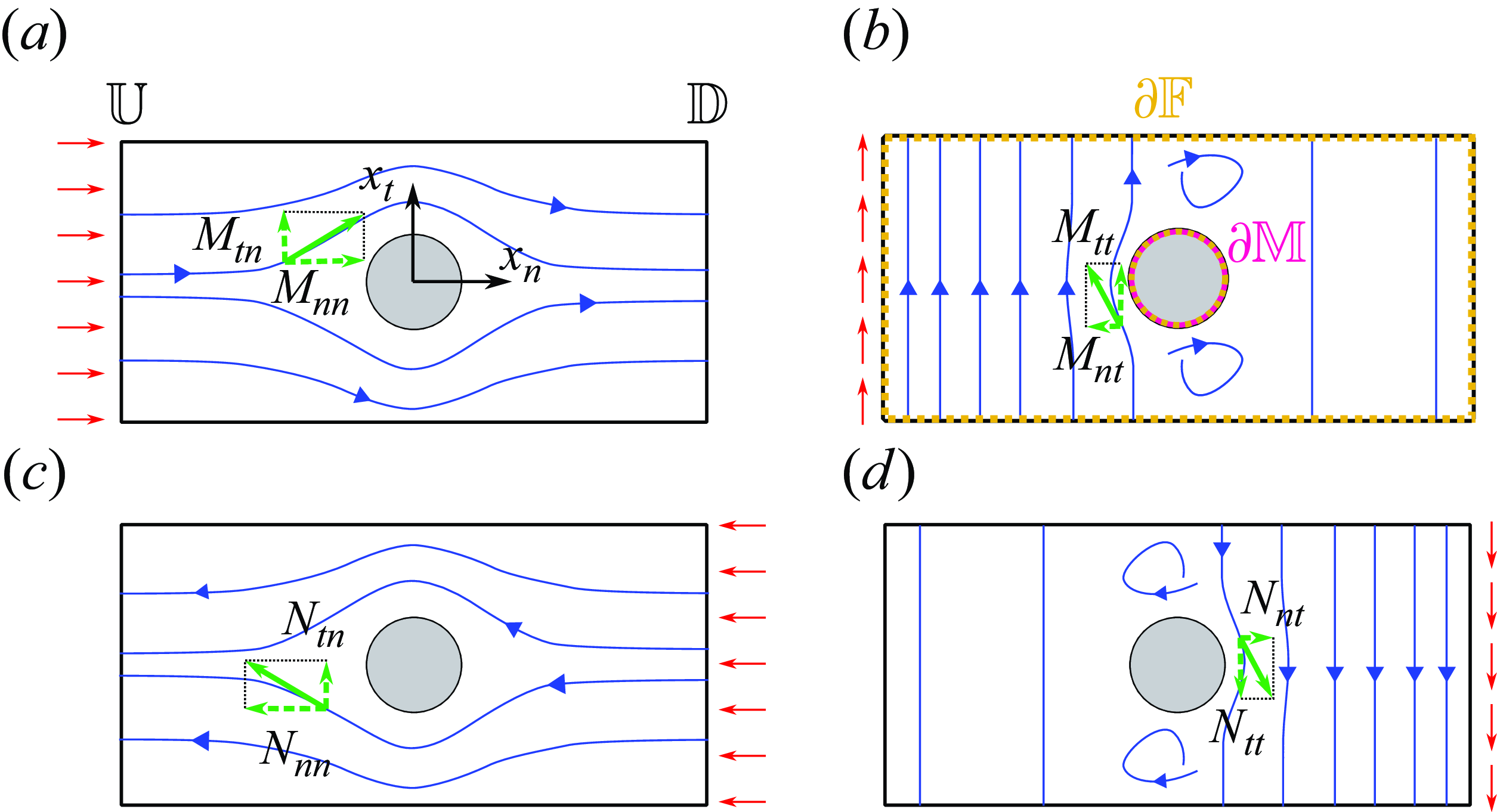
In the case of an aperiodic porous medium satisfying a precise set of hypotheses based on statistics, such as ergodicity, it is possible to apply homogenisation within a REV. The REV can be regarded as the minimal subset of the medium at which some properties, such as its porosity or the permeability, are statistically constant if the subset size is enlarged (Bear & Bachmat Reference Bear and Bachmat1990). We denote with $l'$
(cf. figure 1
$l'$
(cf. figure 1 $c$
) the REV size, with
$c$
) the REV size, with $l$
the distance between two subsequent pore centres and
$l$
the distance between two subsequent pore centres and $L$
the membrane characteristic length. We can estimate that
$L$
the membrane characteristic length. We can estimate that $l'\sim ml$
, where
$l'\sim ml$
, where $m$
is the number of pores we count crossing the REV along some direction. Bear & Bachmat (Reference Bear and Bachmat1990) adopted statistical arguments to conclude the need for the scale relation
$m$
is the number of pores we count crossing the REV along some direction. Bear & Bachmat (Reference Bear and Bachmat1990) adopted statistical arguments to conclude the need for the scale relation $\,l \ll l' \ll L$
. Based on experimental evidence, Auriault et al. (Reference Auriault, Boutin and Geindreau2009) have shown that the relation above is relaxed as
$\,l \ll l' \ll L$
. Based on experimental evidence, Auriault et al. (Reference Auriault, Boutin and Geindreau2009) have shown that the relation above is relaxed as $l \leq l' \ll L$
, where the equality is attained in the case of periodic microstructure, i.e.
$l \leq l' \ll L$
, where the equality is attained in the case of periodic microstructure, i.e. $m=1$
, and the REV reduces to the unit cell. A common choice to compute the permeability associated with some REV geometry is to employ its periodic extension and impose periodic boundary conditions on the fluid flow variables along the membrane tangential directions, compare with, for example, Hendrick et al. (Reference Hendrick, Erdmann and Goodman2012). From a practical point of view, we need to verify that the ergodicity hypothesis at the basis of the REV concept applies to a given microstructure: a strategy to establish which REV is statistically representative of the whole geometry is to calculate the membrane properties in sets of nested REVs and determine when the property of interest converges with the size and location of the REV. Identifying such a REV requires many direct evaluations of the average medium properties. In this paper, we propose an efficient procedure to evaluate the properties of such different REV geometries. To perform this task, we postulate the existence of a REV and we consider simple pore geometries. This procedure can also be applied to explore geometrical modifications of periodic porous media, where the unitary cell replaces the REV.
$m=1$
, and the REV reduces to the unit cell. A common choice to compute the permeability associated with some REV geometry is to employ its periodic extension and impose periodic boundary conditions on the fluid flow variables along the membrane tangential directions, compare with, for example, Hendrick et al. (Reference Hendrick, Erdmann and Goodman2012). From a practical point of view, we need to verify that the ergodicity hypothesis at the basis of the REV concept applies to a given microstructure: a strategy to establish which REV is statistically representative of the whole geometry is to calculate the membrane properties in sets of nested REVs and determine when the property of interest converges with the size and location of the REV. Identifying such a REV requires many direct evaluations of the average medium properties. In this paper, we propose an efficient procedure to evaluate the properties of such different REV geometries. To perform this task, we postulate the existence of a REV and we consider simple pore geometries. This procedure can also be applied to explore geometrical modifications of periodic porous media, where the unitary cell replaces the REV.
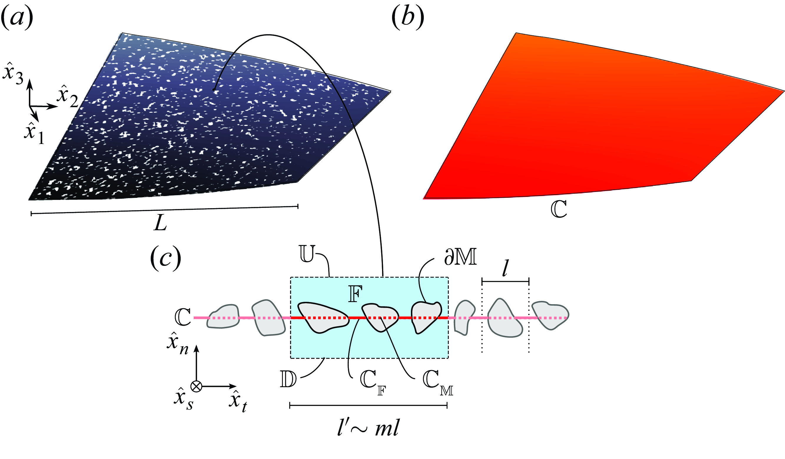
( $a$
) Porous aperiodic thin membrane as it appears in the physical world. We denote with
$a$
) Porous aperiodic thin membrane as it appears in the physical world. We denote with $(\hat {x}_1,\hat {x}_2,\hat {x}_3)$
the (dimensional) global coordinate system and with
$(\hat {x}_1,\hat {x}_2,\hat {x}_3)$
the (dimensional) global coordinate system and with $L$
the characteristic size of the membrane. (
$L$
the characteristic size of the membrane. ( $b$
) Membrane centresurface
$b$
) Membrane centresurface $\mathbb {C}$
, which serves as a fictitious interface to divide the original fluid domain into two macroscopic subdomains. (
$\mathbb {C}$
, which serves as a fictitious interface to divide the original fluid domain into two macroscopic subdomains. ( $c$
) Section of the local aperiodic microstructure of the full-scale membrane, neglecting the curvature of
$c$
) Section of the local aperiodic microstructure of the full-scale membrane, neglecting the curvature of $\mathbb {C}$
.
$\mathbb {C}$
. $(\hat {x}_n,\hat {x}_t,\hat {x}_s)$
is the local coordinate system, aligned with the normal and tangent vectors to the membrane midsurface,
$(\hat {x}_n,\hat {x}_t,\hat {x}_s)$
is the local coordinate system, aligned with the normal and tangent vectors to the membrane midsurface, $\mathbb {C}$
(red). Along the membrane, we identify a REV (dashed black line in the zoom box) of size
$\mathbb {C}$
(red). Along the membrane, we identify a REV (dashed black line in the zoom box) of size $l'$
, which counts
$l'$
, which counts $m$
unit cells of typical size
$m$
unit cells of typical size $l$
(distance between two subsequent pore centres). We denote with
$l$
(distance between two subsequent pore centres). We denote with $\mathbb {F}$
the fluid domain inside it and with
$\mathbb {F}$
the fluid domain inside it and with $\mathbb {U},\mathbb {D}$
and
$\mathbb {U},\mathbb {D}$
and $\partial \mathbb {M}$
its upward and downward sides and its boundary with any solid inclusion, respectively. The portions of the (rectified) membrane centreline
$\partial \mathbb {M}$
its upward and downward sides and its boundary with any solid inclusion, respectively. The portions of the (rectified) membrane centreline $\mathbb {C}$
in the REV crossing the fluid and the solid are denoted with
$\mathbb {C}$
in the REV crossing the fluid and the solid are denoted with $\mathbb {C}_{\mathbb {F}}$
(red line) and
$\mathbb {C}_{\mathbb {F}}$
(red line) and $\mathbb {C}_{\mathbb {M}}$
(red dots), respectively.
$\mathbb {C}_{\mathbb {M}}$
(red dots), respectively.
In our domain, the fluid region in the REV is denoted by $\mathbb {F}$
(figure 1) and all the boundaries of the fluid domain by
$\mathbb {F}$
(figure 1) and all the boundaries of the fluid domain by $\partial \mathbb {F}$
. Among the latter, the solid–fluid boundary is called
$\partial \mathbb {F}$
. Among the latter, the solid–fluid boundary is called $\partial \mathbb {M}$
and the upward and downward sides of
$\partial \mathbb {M}$
and the upward and downward sides of $\mathbb {F}$
are named
$\mathbb {F}$
are named $\mathbb {U}$
and
$\mathbb {U}$
and $\mathbb {D}$
, respectively. The Navier–Stokes equations govern the evolution of the dimensional flow velocity
$\mathbb {D}$
, respectively. The Navier–Stokes equations govern the evolution of the dimensional flow velocity $\hat {u}_i$
and pressure
$\hat {u}_i$
and pressure $\hat {p}$
in the whole fluid domain,
$\hat {p}$
in the whole fluid domain,
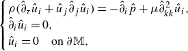 \begin{equation} \begin{cases} \rho (\hat {\partial }_{\tau }\hat {u}_i+\hat {u}_j\hat {\partial }_j \hat {u}_i)=-\hat {\partial }_i \hat {p}+\mu \hat {\partial }_{kk}^2 \hat {u}_i, \\ \hat {\partial }_i \hat {u}_i=0, \\ \hat {u}_i=0 \quad \text {on}\ \partial \mathbb {M}, \end{cases} \end{equation}
where Einstein’s index notation is adopted and $\hat {u}_i=0$
is intended for each vector component.
$\hat {u}_i=0$
is intended for each vector component.
Zampogna & Gallaire (Reference Zampogna and Gallaire2020) proposed a predictive homogeneous model to compute the average flow fields across a periodic thin membrane. In this model, the membrane is treated as a fictitious interface on which equivalent stress-jump conditions are imposed to mimic the macroscopic effect of the real porous structure on the fluid flow. These conditions, explicitly given in § 2.1.5, contain some coefficients which represent the membrane properties and are the solution of Stokes problems within the REV. We summarise the homogenised model in § 2.1 and introduce in § 2.2 the adjoint-based method used to compute the sensitivity of the above-mentioned coefficients with respect to shape changes.
2.1. From the pore geometry to the macroscopic flow
Starting from the Navier–Stokes equations (2.1), the homogenisation procedure described in Zampogna & Gallaire (Reference Zampogna and Gallaire2020) relies on the following steps: (i) define and normalise the inner equations, valid at the pore scale, (ii) define and normalize the outer equations, valid far from the membrane, (iii) match the inner and outer equations and solve the inner (microscopic) problem and (iv) average the inner solution and deduce the macroscopic conditions, i.e. the equivalent interface conditions to account for the presence of the membrane in the outer (macroscopic) problem. In the present analysis, we develop a new methodology to efficiently compute the average solution of the microscopic problems for different microstructures. We thus consider a small number of pores per REV, i.e. $m= \mathcal{O}(1)$
(when
$m= \mathcal{O}(1)$
(when $m=1$
, we have a fully periodic geometry). We introduce a small scale-separation parameter
$m=1$
, we have a fully periodic geometry). We introduce a small scale-separation parameter $\epsilon =l/L$
, that is the ratio between the typical interpore distance and the membrane characteristic size. Auriault et al. (Reference Auriault, Boutin and Geindreau2009) suggested that real heterogeneous media exhibit a typical
$\epsilon =l/L$
, that is the ratio between the typical interpore distance and the membrane characteristic size. Auriault et al. (Reference Auriault, Boutin and Geindreau2009) suggested that real heterogeneous media exhibit a typical $m$
of approximately
$m$
of approximately $10$
. The relevant separation of scales parameter
$10$
. The relevant separation of scales parameter $\epsilon$
is not modified by the introduction of a REV of typical size
$\epsilon$
is not modified by the introduction of a REV of typical size $l'$
, since
$l'$
, since $l\sim l'$
. The relation
$l\sim l'$
. The relation $\epsilon =l/L\sim l'/L$
holds, which is consistent with considering a small number of pores per REV.
$\epsilon =l/L\sim l'/L$
holds, which is consistent with considering a small number of pores per REV.
2.1.1. The inner, pore-scale problem
We first focus on the inner, pore-scale flow description within the REV. We introduce the following non-dimensionalisation for equation (2.1):
 \begin{equation} \hat {x}_i=l x_i \qquad \hat {p}=\Delta P p=\frac {\mu U}{l}p \qquad \hat {u}_i=Uu_i \qquad \hat {\tau }=T\tau =\frac {l}{U}\tau , \end{equation}
where $\Delta P$
and
$\Delta P$
and $U$
are the (dimensional) microscale characteristic pressure difference and microscale velocity, respectively. The governing equations become
$U$
are the (dimensional) microscale characteristic pressure difference and microscale velocity, respectively. The governing equations become
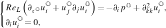
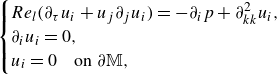 \begin{equation} \begin{cases} Re_l(\partial _{\tau } u_i+u_j\partial _j u_i)=-\partial _i p+ \partial _{kk}^2 u_i, \\ \partial _i u_i=0, \\ u_i=0 \quad \text {on $\partial \mathbb {M}$}, \end{cases} \end{equation}
where $Re_l=\rho U l/\mu$
is the Reynolds number based on the microscopic length
$Re_l=\rho U l/\mu$
is the Reynolds number based on the microscopic length $l$
and microscale characteristic velocity
$l$
and microscale characteristic velocity $U$
. We assume that the flow variables
$U$
. We assume that the flow variables $(u_i,p)$
exhibit periodicity along the tangential-to-the-membrane direction in the REV, but not at the macroscale, i.e. they are locally periodic but macroscopically aperiodic. This approach has already been proposed for homogenizing fluid flows and solute transport across bulk, heterogeneous porous media by, for example, Dalwadi et al. (Reference Dalwadi, Griffiths and Bruna2015) and Auton et al. (Reference Auton, Pramanik, Dalwadi, MacMinn and Griffiths2022).
$(u_i,p)$
exhibit periodicity along the tangential-to-the-membrane direction in the REV, but not at the macroscale, i.e. they are locally periodic but macroscopically aperiodic. This approach has already been proposed for homogenizing fluid flows and solute transport across bulk, heterogeneous porous media by, for example, Dalwadi et al. (Reference Dalwadi, Griffiths and Bruna2015) and Auton et al. (Reference Auton, Pramanik, Dalwadi, MacMinn and Griffiths2022).
2.1.2. The outer, membrane-scale problem
In the macroscopic domain, the following non-dimensionalisation is employed to scale the equations:
 \begin{equation} \hat {x}_i=L X_i \qquad \hat {p}=\Delta P^{\mathbb {O}} p^{\mathbb {O}}=\frac {\mu U^{\mathbb {O}}}{L} p^{\mathbb {O}}, \qquad \hat {u}_i=U^{\mathbb {O}} u^{\mathbb {O}}_i, \qquad \hat {\tau }=T^{\mathbb {O}} \tau ^{\mathbb {O}}=\frac {L}{U^{\mathbb {O}}}\tau ^{\mathbb {O}}, \end{equation}
where $\Delta P^{\mathbb {O}}, U^{\mathbb {O}}$
and
$\Delta P^{\mathbb {O}}, U^{\mathbb {O}}$
and $T^{\mathbb {O}}$
are the (dimensional) outer pressure difference, velocity and time scales, respectively. The governing equations of the outer problem become
$T^{\mathbb {O}}$
are the (dimensional) outer pressure difference, velocity and time scales, respectively. The governing equations of the outer problem become
 \begin{equation} \begin{cases} Re_L\left (\partial _{{\tau ^{\mathbb {O}}}}u_i^{\mathbb {O}}+u_j^{\mathbb {O}}\partial _j u_i^{\mathbb {O}}\right )=-\partial _i p^{\mathbb {O}}+ \partial _{kk}^2 u^{\mathbb {O}}_i, \\ \partial _i u^{\mathbb {O}}_i=0, \end{cases} \end{equation}
where $Re_L=\rho U^{\mathbb {O}}L/\mu$
is the Reynolds number based on the macroscopic length
$Re_L=\rho U^{\mathbb {O}}L/\mu$
is the Reynolds number based on the macroscopic length $L$
and outer velocity
$L$
and outer velocity $U^{\mathbb {O}}$
.
$U^{\mathbb {O}}$
.
2.1.3. Matching inner and outer normalisations
On the upward $\mathbb {U}$
and downward
$\mathbb {U}$
and downward $\mathbb {D}$
sides of the fluid domain
$\mathbb {D}$
sides of the fluid domain $\mathbb {F}$
, the fluid flow is continuous, i.e. the (dimensional) velocity and fluid stresses match
$\mathbb {F}$
, the fluid flow is continuous, i.e. the (dimensional) velocity and fluid stresses match
 \begin{equation} u_i U=u_i^{\mathbb {O,U}} U^{\mathbb {O}},\quad u_i U=u_i^{\mathbb {O,D}} U^{\mathbb {O}},\quad \Sigma _{ij}n_j=\epsilon \frac {U^{\mathbb {O}}}{U}\Sigma ^{\mathbb {O,U}}_{ij}n_j ,\quad \Sigma _{ij}n_j=\epsilon \frac {U^{\mathbb {O}}}{U}\Sigma ^{\mathbb {O,D}}_{ij}n_j, \end{equation}
where $\Sigma _{ij}=-p\delta _{ij}+(\partial _i u_j +\partial _j u_i)$
is the stress tensors normalised with the inner scales and
$\Sigma _{ij}=-p\delta _{ij}+(\partial _i u_j +\partial _j u_i)$
is the stress tensors normalised with the inner scales and $\Sigma _{ij}^{\mathbb {O},\mathbb {U}}=-p^{\mathbb {O},\mathbb {U}}\delta _{ij}+(\partial _i u_j^{\mathbb {O},\mathbb {U}} +\partial _j u_i^{\mathbb {O},\mathbb {U}})$
and
$\Sigma _{ij}^{\mathbb {O},\mathbb {U}}=-p^{\mathbb {O},\mathbb {U}}\delta _{ij}+(\partial _i u_j^{\mathbb {O},\mathbb {U}} +\partial _j u_i^{\mathbb {O},\mathbb {U}})$
and $\Sigma _{ij}^{\mathbb {O},\mathbb {D}}=-p^{\mathbb {O},\mathbb {D}}\delta _{ij}+(\partial _i u_j^{\mathbb {O},\mathbb {D}} +\partial _j u_i^{\mathbb {O},\mathbb {D}})$
are the stress tensors normalised with the outer scales and evaluated on
$\Sigma _{ij}^{\mathbb {O},\mathbb {D}}=-p^{\mathbb {O},\mathbb {D}}\delta _{ij}+(\partial _i u_j^{\mathbb {O},\mathbb {D}} +\partial _j u_i^{\mathbb {O},\mathbb {D}})$
are the stress tensors normalised with the outer scales and evaluated on $\mathbb {U}$
or
$\mathbb {U}$
or $\mathbb {D}$
, respectively.
$\mathbb {D}$
, respectively.
2.1.4. Solving the inner problem
Exploiting the separation between the pore and membrane length scales, we can decompose the inner spatial variable into a fast ( $x_i$
) and a slow (
$x_i$
) and a slow ( $X_i$
) variable and perform an asymptotic expansion of the flow fields,
$X_i$
) variable and perform an asymptotic expansion of the flow fields,
 \begin{equation} x_i\rightarrow x_i+\epsilon X_i, \quad \partial _i\rightarrow \partial _i+\epsilon \partial _I, \quad (u_i,p)\rightarrow (u_i^{(0)},p^{(0)})+\epsilon (u_i^{(1)},p^{(1)})+O(\epsilon ^2), \end{equation}
where the capital subscript denotes the derivation with respect to the macroscopic slow spatial variable $X_i$
. Substituting (2.7) into (2.3), supposing that the flow inertia is negligible at the pore scale (as in Malone et al. Reference Malone, Hutchinson and Prager1974; Tio & Sadhal Reference Tio and Sadhal1994; Zampogna & Gallaire Reference Zampogna and Gallaire2020; Ledda et al. Reference Ledda, Boujo, Camarri, Gallaire and Zampogna2021; Zampogna et al. Reference Zampogna, Ledda, Wittkowski and Gallaire2023), i.e.
$X_i$
. Substituting (2.7) into (2.3), supposing that the flow inertia is negligible at the pore scale (as in Malone et al. Reference Malone, Hutchinson and Prager1974; Tio & Sadhal Reference Tio and Sadhal1994; Zampogna & Gallaire Reference Zampogna and Gallaire2020; Ledda et al. Reference Ledda, Boujo, Camarri, Gallaire and Zampogna2021; Zampogna et al. Reference Zampogna, Ledda, Wittkowski and Gallaire2023), i.e. $Re_l\sim \epsilon$
, and collecting each order term in
$Re_l\sim \epsilon$
, and collecting each order term in $\epsilon$
, we obtain the leading-order problem
$\epsilon$
, we obtain the leading-order problem
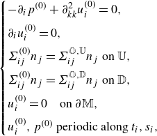 \begin{equation} \begin{cases} -\partial _i p^{(0)}+ \partial _{kk}^2 u_i^{(0)}=0,\\[5pt] \partial _i u_i^{(0)}=0,\\[5pt] \Sigma _{ij}^{(0)}n_j=\Sigma _{ij}^{\mathbb {O,U}}n_j \text { on $\mathbb {U}$},\\[5pt] \Sigma _{ij}^{(0)}n_j=\Sigma _{ij}^{\mathbb {O,D}}n_j \text { on $\mathbb {D}$},\\[5pt] u_i^{(0)}=0 \quad \text {on } \partial \mathbb {M},\\[5pt] u_i^{(0)},p^{(0)} \text { periodic along } t_i, s_i, \end{cases} \end{equation}
where $t_i,s_i$
are the tangents to the membrane centreline
$t_i,s_i$
are the tangents to the membrane centreline $\mathbb {C}$
(cf. figure 1
$\mathbb {C}$
(cf. figure 1 $b,\!c$
). In problem (2.8), the quantities
$b,\!c$
). In problem (2.8), the quantities $\Sigma _{jk}^{\mathbb {O,U}}$
and
$\Sigma _{jk}^{\mathbb {O,U}}$
and $\Sigma _{jk}^{\mathbb {O,D}}$
do not depend on the integration variable
$\Sigma _{jk}^{\mathbb {O,D}}$
do not depend on the integration variable $x_i$
and they act as non-homogeneous source terms. As shown by Zampogna & Gallaire (Reference Zampogna and Gallaire2020), the linearity of the governing equations allows us to formally write the velocity and pressure fields as a linear combination of the source terms, i.e. the outer stresses acting on the upward
$x_i$
and they act as non-homogeneous source terms. As shown by Zampogna & Gallaire (Reference Zampogna and Gallaire2020), the linearity of the governing equations allows us to formally write the velocity and pressure fields as a linear combination of the source terms, i.e. the outer stresses acting on the upward $\mathbb {U}$
and downward
$\mathbb {U}$
and downward $\mathbb {D}$
sides of the REV. Naming
$\mathbb {D}$
sides of the REV. Naming $M_{ij},N_{ij},Q_j$
and
$M_{ij},N_{ij},Q_j$
and $R_j$
the coefficients of the linear combination, the formal solution of problem (2.8) is written as
$R_j$
the coefficients of the linear combination, the formal solution of problem (2.8) is written as
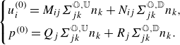 \begin{equation} \begin{cases} u_i^{(0)}=M_{ij}\Sigma _{jk}^{\mathbb {O,U}}n_k+N_{ij}\Sigma _{jk}^{\mathbb {O,D}}n_k,\\[5pt] p^{(0)}=Q_{j}\Sigma _{jk}^{\mathbb {O,U}}n_k+R_{j}\Sigma _{jk}^{\mathbb {O,D}}n_k. \end{cases} \end{equation}
Substituting (2.9) into (2.8), we obtain the closure problems (the so-called microscopic problems) for the quantities $M_{ij},N_{ij},Q_j$
and
$M_{ij},N_{ij},Q_j$
and $R_j$
within the REV, i.e.
$R_j$
within the REV, i.e.
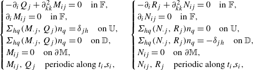 \begin{equation} \begin{cases} -\partial _i Q_{j} +\partial ^2_{kk}M_{ij}=0 \quad \text {in $\mathbb {F}$},\\ \partial _i M_{ij}=0 \quad \text {in $\mathbb {F}$},\\ \Sigma _{hq}(M_{\cdot j},Q_{j})n_q=\delta _{jh} \quad \text {on $\mathbb {U}$},\\ \Sigma _{hq}(M_{\cdot j},Q_{j})n_q=0 \quad \text {on $\mathbb {D}$},\\ M_{ij}=0 \quad \text {on $\partial \mathbb {M}$},\\ M_{ij},Q_{j} \quad \text {periodic along $t_i$,$s_i$}, \end{cases} \begin{cases} -\partial _i R_{j} +\partial ^2_{kk}N_{ij}=0 \quad \text {in $\mathbb {F}$},\\ \partial _i N_{ij}=0 \quad \text {in $\mathbb {F}$},\\ \Sigma _{hq}(N_{\cdot j},R_{j})n_q=0 \quad \text {on $\mathbb {U}$},\\ \Sigma _{hq}(N_{\cdot j},R_{j})n_q={-}\delta _{jh} \quad \text {on $\mathbb {D}$},\\ N_{ij}=0 \quad \text {on $\partial \mathbb {M}$},\\ N_{ij},R_{j} \quad \text {periodic along $t_i$,$s_i$}, \end{cases} \end{equation}
where $\delta _{jh}$
is the Kronecker delta and we adopt the notation
$\delta _{jh}$
is the Kronecker delta and we adopt the notation $\Sigma _{hq}(A_{\cdot j},B_{j})=- B_j \delta _{hq}+(\partial _h A_{qj}+\partial _q A_{hj})$
, that is, fixing
$\Sigma _{hq}(A_{\cdot j},B_{j})=- B_j \delta _{hq}+(\partial _h A_{qj}+\partial _q A_{hj})$
, that is, fixing $j$
, the dimensionless stress tensor built from
$j$
, the dimensionless stress tensor built from $B_j$
acting as pressure and
$B_j$
acting as pressure and $A_{\cdot j}$
as velocity field.
$A_{\cdot j}$
as velocity field.
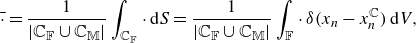
For the sake of clarity, we describe the physical significance of the entries of the quantities $M_{ij},N_{ij},Q_j$
and
$M_{ij},N_{ij},Q_j$
and $R_j$
for the two-dimensional (2-D) configuration depicted in figure 2. We thus forget for a moment about the
$R_j$
for the two-dimensional (2-D) configuration depicted in figure 2. We thus forget for a moment about the $s$
components and focus on the
$s$
components and focus on the $n,t$
ones. For a fixed
$n,t$
ones. For a fixed $j$
, the vector field
$j$
, the vector field $M_{ij}$
(
$M_{ij}$
( $N_{ij}$
) and the scalar field
$N_{ij}$
) and the scalar field $Q_j$
(
$Q_j$
( $R_j$
) play the role of flow velocity and pressure in a problem governed by Stokes’s flow with no-slip boundary conditions on the fluid–solid interface
$R_j$
) play the role of flow velocity and pressure in a problem governed by Stokes’s flow with no-slip boundary conditions on the fluid–solid interface $\partial \mathbb {M}$
, periodicity along the tangential direction and an external unitary stress applied along the normal – if
$\partial \mathbb {M}$
, periodicity along the tangential direction and an external unitary stress applied along the normal – if $j=n$
– or tangential – if
$j=n$
– or tangential – if $j=t$
– direction on the upward
$j=t$
– direction on the upward $\mathbb {U}$
(downward
$\mathbb {U}$
(downward $\mathbb {D}$
) side of the domain. Thus,
$\mathbb {D}$
) side of the domain. Thus, $M_{\cdot n}$
and
$M_{\cdot n}$
and $M_{\cdot t}$
(
$M_{\cdot t}$
( $N_{\cdot n}$
and
$N_{\cdot n}$
and $N_{\cdot t}$
) represent the flow field caused by normal and tangential unitary stresses applied on
$N_{\cdot t}$
) represent the flow field caused by normal and tangential unitary stresses applied on $\mathbb {U}$
(
$\mathbb {U}$
( $\mathbb {D}$
), respectively. Similarly,
$\mathbb {D}$
), respectively. Similarly, $Q_n$
and
$Q_n$
and $Q_t$
(
$Q_t$
( $R_n$
and
$R_n$
and $R_t$
) represent the pressure fields caused by normal and tangential unitary stress on
$R_t$
) represent the pressure fields caused by normal and tangential unitary stress on $\mathbb {U}$
(
$\mathbb {U}$
( $\mathbb {D}$
), respectively.
$\mathbb {D}$
), respectively.
Sketch showing the physical meaning of $M_{ij}$
and
$M_{ij}$
and $N_{ij}$
. A 2-D configuration is chosen, with a membrane formed by the periodical repetition of circular solid inclusions. In each panel, the left-hand and right-hand sides of the rectangular cell,
$N_{ij}$
. A 2-D configuration is chosen, with a membrane formed by the periodical repetition of circular solid inclusions. In each panel, the left-hand and right-hand sides of the rectangular cell, $\mathbb {U,D}$
, are the upward and downward sides of the fluid domain
$\mathbb {U,D}$
, are the upward and downward sides of the fluid domain $\mathbb {F}$
as in figure 1(
$\mathbb {F}$
as in figure 1( $c$
). The union of all fluid boundaries,
$c$
). The union of all fluid boundaries, $\partial \mathbb {F}$
, and the fluid–solid boundary alone,
$\partial \mathbb {F}$
, and the fluid–solid boundary alone, $\partial \mathbb {M}$
, are shown in (b) in yellow and magenta, respectively. The red arrows represent the direction of the vector
$\partial \mathbb {M}$
, are shown in (b) in yellow and magenta, respectively. The red arrows represent the direction of the vector $\Sigma _{ij}n_j$
, while the blue lines represent the flow streamlines. Solid green arrows represent the local flow direction and the corresponding dashed arrows its components along the principal axes: (a)
$\Sigma _{ij}n_j$
, while the blue lines represent the flow streamlines. Solid green arrows represent the local flow direction and the corresponding dashed arrows its components along the principal axes: (a) $(M_{nn},M_{tn})$
; (b)
$(M_{nn},M_{tn})$
; (b) $(M_{nt},M_{tt})$
; (c)
$(M_{nt},M_{tt})$
; (c) $(N_{nn},N_{tn})$
; (d)
$(N_{nn},N_{tn})$
; (d) $(N_{nt},N_{tt})$
.
$(N_{nt},N_{tt})$
.
However, to represent the effect of the membrane microstructure, we are interested in the average values of these tensor quantities. Indeed, the average value of $M_{nn}$
can be interpreted as a permeability coefficient and the average value of
$M_{nn}$
can be interpreted as a permeability coefficient and the average value of $M_{tt}$
as a slip coefficient, for example (Zampogna & Gallaire Reference Zampogna and Gallaire2020).
$M_{tt}$
as a slip coefficient, for example (Zampogna & Gallaire Reference Zampogna and Gallaire2020).
2.1.5. The macroscopic conditions
Model (2.9) together with the microscopic problems (2.10) represent a closed description for the flow in the vicinity of the membrane. However, (2.9) still contains the dependence on the microscopic spatial variable $x_i$
, since
$x_i$
, since $M_{ij},N_{ij},Q_j$
and
$M_{ij},N_{ij},Q_j$
and $R_j$
depend on it. Our objective is to find an interface condition which depends only on the macroscopic spatial variable
$R_j$
depend on it. Our objective is to find an interface condition which depends only on the macroscopic spatial variable $X_i$
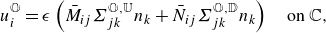
. To obtain the membrane macroscopic model, we introduce the spatial average
$X_i$
. To obtain the membrane macroscopic model, we introduce the spatial average
 \begin{equation} \bar {\cdot } =\frac {1}{|\mathbb {C}_{\mathbb {F}}\cup \mathbb {C}_{\mathbb {M}}|}\int _{\mathbb {C}_{\mathbb {F}}}\cdot \,{\rm d}S =\frac {1}{|\mathbb {C}_{\mathbb {F}}\cup \mathbb {C}_{\mathbb {M}}|} \int _{\mathbb {F}} \cdot \, \delta (x_n-x_n^{\mathbb {C}}) \,{\rm d}V, \end{equation}
where $\delta (x_n-x_n^{\mathbb {C}})$
is the Dirac delta centred in
$\delta (x_n-x_n^{\mathbb {C}})$
is the Dirac delta centred in $x_n^{\mathbb {C}}$
,
$x_n^{\mathbb {C}}$
, $dS$
and
$dS$
and $dV$
are an infinitesimal element of surface and volume, respectively, and
$dV$
are an infinitesimal element of surface and volume, respectively, and $\cdot$
represents any of the entries in
$\cdot$
represents any of the entries in $M_{ij},N_{ij},Q_j$
or
$M_{ij},N_{ij},Q_j$
or $R_j$
, solution of (2.10) and
$R_j$
, solution of (2.10) and $\mathbb {C}_{\mathbb {F}}$
and
$\mathbb {C}_{\mathbb {F}}$
and $\mathbb {C}_{\mathbb {M}}$
represent the fluid and solid portion of the membrane centreline
$\mathbb {C}_{\mathbb {M}}$
represent the fluid and solid portion of the membrane centreline $\mathbb {C}$
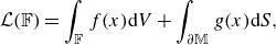
(cf. figure 1). Applying average (2.11) to (2.9) and renormalizing with the outer scales, we obtain the purely macroscopic conditions
$\mathbb {C}$
(cf. figure 1). Applying average (2.11) to (2.9) and renormalizing with the outer scales, we obtain the purely macroscopic conditions
 \begin{equation} u_i^{\mathbb {O}}=\epsilon \left (\bar {M}_{ij}\Sigma _{jk}^{\mathbb {O,U}}n_k+\bar {N}_{ij}\Sigma _{jk}^{\mathbb {O,D}}n_k\right ) \quad \text {on $ \mathbb {C}$}, \end{equation}
 \begin{equation} p^{\mathbb {O}}=\bar {Q}_{j}\Sigma _{jk}^{\mathbb {O,U}}n_k+\bar {R}_{j}\Sigma _{jk}^{\mathbb {O,D}}n_k \quad \text {on $\mathbb {C}$}. \end{equation}
These equivalent interface conditions quantify the effects of the porous membrane on the flow from a purely macroscopic perspective, without the need to solve the fluid flow in the geometric details of the membrane for each specific flow configuration. The effect of the microstructure is indeed entirely embedded in the tensors $\bar {M}_{ij}, \bar {N}_{ij}$
, known as Navier tensors (Zampogna & Gallaire Reference Zampogna and Gallaire2020), while the vectors
$\bar {M}_{ij}, \bar {N}_{ij}$
, known as Navier tensors (Zampogna & Gallaire Reference Zampogna and Gallaire2020), while the vectors $\bar {Q}_j$
and
$\bar {Q}_j$
and $\bar {R}_j$
are only useful to estimate the pressure on the membrane centreline a posteriori, if needed. If the membrane microstructure is periodic, we need to solve the microscopic problem (2.10) once and for all to find the averaged quantities, whereas when the microstructure is non-periodic, in principle, we should solve system (2.10) within each REV. This negatively affects the computational efficiency of the method. In the following, we develop a sensitivity-based procedure to perform this operation with a computational cost similar to the periodic case, independently of the number of REVs. We focus on the microscopic problem (2.10) that defines the Navier tensors and on the adjoint problems needed to compute the sensitivity of these tensors to changes in the geometry of the solid inclusion’s boundary
$\bar {R}_j$
are only useful to estimate the pressure on the membrane centreline a posteriori, if needed. If the membrane microstructure is periodic, we need to solve the microscopic problem (2.10) once and for all to find the averaged quantities, whereas when the microstructure is non-periodic, in principle, we should solve system (2.10) within each REV. This negatively affects the computational efficiency of the method. In the following, we develop a sensitivity-based procedure to perform this operation with a computational cost similar to the periodic case, independently of the number of REVs. We focus on the microscopic problem (2.10) that defines the Navier tensors and on the adjoint problems needed to compute the sensitivity of these tensors to changes in the geometry of the solid inclusion’s boundary $\partial \mathbb {M}$
.
$\partial \mathbb {M}$
.
2.1.6. Further considerations on the Navier tensors
A few considerations are propaedeutic for a better comprehension of the adjoint analysis which we will perform in the next section.
-
(i) The macroscopic problem (2.5) and the boundary condition (2.12) determine the outer macroscopic solution $(u_i^{\mathbb {O}}, p^{\mathbb {O}})$
, including
$p^{\mathbb {O}}$
on each side of the membrane;
$Q_j$
and
$R_j$
are only needed if one wishes to evaluate a posteriori
$p^{\mathbb {O}}$
at the membrane centreline with (2.13). Therefore, we will use the adjoint-based sensitivity to estimate the effect of inclusion geometry changes on
$M_{ij}$
and
$N_{ij}$
only, i.e. we will compute the gradient of the quantities
$\bar {M}_{ij}$
and
$\bar {N}_{ij}$
for a shape modification of the boundary
$\partial \mathbb {M}$
by introducing a Lagrangian optimisation problem and deriving adjoint problems for these quantities. The method can easily be adapted to estimate the effect on
$Q_j$
and
$R_j$
, but it is not necessary for the determination of the flow across the membrane.
$(u_i^{\mathbb {O}}, p^{\mathbb {O}})$
, including
$p^{\mathbb {O}}$
on each side of the membrane;
$Q_j$
and
$R_j$
are only needed if one wishes to evaluate a posteriori
$p^{\mathbb {O}}$
at the membrane centreline with (2.13). Therefore, we will use the adjoint-based sensitivity to estimate the effect of inclusion geometry changes on
$M_{ij}$
and
$N_{ij}$
only, i.e. we will compute the gradient of the quantities
$\bar {M}_{ij}$
and
$\bar {N}_{ij}$
for a shape modification of the boundary
$\partial \mathbb {M}$
by introducing a Lagrangian optimisation problem and deriving adjoint problems for these quantities. The method can easily be adapted to estimate the effect on
$Q_j$
and
$R_j$
, but it is not necessary for the determination of the flow across the membrane. -
(ii) In the particular case of solid inclusions that are symmetric about the membrane centreline
$\mathbb {C}$
, the Navier tensors satisfy(2.14)In the specific configuration of solid inclusions that are also symmetric about the normal membrane direction, then
\begin{equation} \bar {N}_{ij}=-\bar {M}_{ij}. \end{equation}
$\bar {M}_{nt}=\bar {M}_{tn}=0$
.
-
(iii) Equations (2.10) are a set of Stokes problems normally (
$j=n$
) or tangentially (
$j=t$
or
$s$
) forced on the upward side
$\mathbb {U}$
or downward side
$\mathbb {D}$
of the fluid domain
$\mathbb {F}$
(for
$M_{ij}$
or
$N_{ij}$
, respectively). Equation (2.10) is essentially a set of three independent problems for
$M_{ij}$
and three for
$N_{ij}$
(i.e. one for each value of the
$j$
subscript). To ease the notation, we rewrite (2.10) column by column by introducing the quantities
$(v_i,q)$
such that(2.15)where
\begin{equation} \begin{cases} -\partial _i q +\partial ^2_{kk}v_i=0 \quad \text {in $\mathbb {F}$},\\ \partial _i v_i=0 \quad \text {in $\mathbb {F}$},\\ \Sigma _{ij}(v_\cdot ,q) n_j=a_i \quad \text {on $\mathbb {U}$},\\ \Sigma _{ij}(v_\cdot ,q) n_j={-}b_i \quad \text {on $\mathbb {D}$},\\ v_i=0 \quad \text {on $\partial \mathbb {M}$},\\ v_i,q \quad \text {periodic along $t_i$,$s_i$}, \end{cases} \end{equation}
(2.16)
\begin{align} a_i=(1,0,0), \, b_i=0 \text { for } M_{\cdot n},Q_n, \qquad & a_i=0, \, b_i=(1,0,0) \text { for } N_{\cdot n},R_n, \end{align}
(2.17)
\begin{align} a_i=(0,1,0), \, b_i=0 \text { for } M_{\cdot t},Q_t, \qquad & a_i=0, \, b_i=(0,1,0) \text { for } N_{\cdot t},Q_t, \end{align}
(2.18)
\begin{align} a_i=(0,0,1), \, b_i=0 \text { for } M_{\cdot s},Q_s, \qquad & a_i=0, \, b_i=(0,0,1) \text { for } N_{\cdot s},R_s, \end{align}
and
$ \Sigma _{ij}(v_{\cdot },q)=-q\delta _{ij}+(\partial _i v_j +\partial _j v_i)$
. This gives a total of six independent Stokes problems, which correspond to (2.10). Explicit correspondence between (2.10) and (2.15) is given in appendix B. In the following section, we use the compact form (2.15) to formally write the sensitivity to solid inclusions shape variations.


2.2. Sensitivity to shape changes in the microscopic geometry
In this section, we derive the first- and second-order shape sensitivities of the Navier tensors. The shape sensitivity is a quantity derived from the original microscopic flow and used to estimate the effect of geometric modifications without recomputing the flow past any modified geometry. In particular, we aim to estimate the change in the Navier tensors induced by a local geometric modification of the porous microstructure in order to understand how this local modification affects the macroscale flow. We follow the formal method of Céa (Reference Céa1986). The reader interested in shape optimisation is referred to Chapter 4 of Allaire et al. (Reference Allaire, Dapogny, Jouve, Bonito and Nochetto2021).
We first recall a general result about shape derivatives. Consider a real-valued functional,
 \begin{equation} \mathcal {L}(\mathbb {F}) = \int _{\mathbb {F}} f(x) {\rm d}V + \int _{\partial \mathbb {M}} g(x) {\rm d}S, \end{equation}
where $f$
and
$f$
and $g$
are sufficiently smooth functions defined on the domain
$g$
are sufficiently smooth functions defined on the domain $\mathbb {F}$
and on part of its boundary
$\mathbb {F}$
and on part of its boundary $\partial \mathbb {M} \subset \partial \mathbb {F}$
, respectively. The shape derivative of
$\partial \mathbb {M} \subset \partial \mathbb {F}$
, respectively. The shape derivative of $\mathcal {L}(\mathbb {F})$
is
$\mathcal {L}(\mathbb {F})$
is
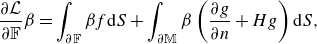 \begin{equation} \dfrac {\partial \mathcal {L}}{\partial \mathbb {F}}\beta = \int _{\partial \mathbb {F}} \beta f {\rm d}S + \int _{\partial \mathbb {M}} \beta \left ( \frac {\partial g}{\partial n} + H g \right ){\rm d}S, \end{equation}
where $\beta (x)$
is the amplitude of the deformation applied to boundary
$\beta (x)$
is the amplitude of the deformation applied to boundary $\partial \mathbb {M}$
perpendicularly to it at any point,
$\partial \mathbb {M}$
perpendicularly to it at any point, $n$
is the normal to
$n$
is the normal to $\partial \mathbb {M}$
, and
$\partial \mathbb {M}$
, and $H=\partial _i n_i$
is the mean curvature of
$H=\partial _i n_i$
is the mean curvature of $\partial \mathbb {M}$
(see e.g. § 5.9 in Henrot & Pierre Reference Henrot and Pierre2005 or § 4.2 in Allaire et al. 2021).
$\partial \mathbb {M}$
(see e.g. § 5.9 in Henrot & Pierre Reference Henrot and Pierre2005 or § 4.2 in Allaire et al. 2021).
2.2.1. First-order sensitivity
We wish to evaluate the effect of a small-amplitude modification of the shape of an inclusion on the spatially averaged Navier tensors $\bar M{_{ij}}$
and
$\bar M{_{ij}}$
and $\bar N{_{ij}}$
, which appear in the effective macroscopic boundary condition (2.12). With the compact form introduced in § 2.1.6, each row of
$\bar N{_{ij}}$
, which appear in the effective macroscopic boundary condition (2.12). With the compact form introduced in § 2.1.6, each row of $M{_{ij}}$
and
$M{_{ij}}$
and $ N{_{ij}}$
is a vector
$ N{_{ij}}$
is a vector $v_i$
solution of the general problem (2.15), made specific to the row of interest with a suitable choice of
$v_i$
solution of the general problem (2.15), made specific to the row of interest with a suitable choice of $a_i$
and
$a_i$
and $b_i$
(see also appendix B). Therefore, we focus on
$b_i$
(see also appendix B). Therefore, we focus on $\bar {v}_i$
, the spatial average of
$\bar {v}_i$
, the spatial average of $v_i$
(as defined in (2.11)), and consider the objective function
$v_i$
(as defined in (2.11)), and consider the objective function $J^{(1)}$
defined as
$J^{(1)}$
defined as
 \begin{equation} J^{(1)}(v_i, \mathbb {F}) = \bar {v}_i r_i = \frac {1}{|\mathbb {C}_{\mathbb {F}}\cup \mathbb {C}_{\mathbb {M}}|} \int _{\mathbb {F}} v_i r_i \delta (x_n-x_n^{\mathbb {C}}){\rm d}V. \end{equation}
Here $r_i$
is a unit vector defined in the
$r_i$
is a unit vector defined in the $(x_n,x_t,x_s)$
microscopic reference frame and used to select a specific component of
$(x_n,x_t,x_s)$
microscopic reference frame and used to select a specific component of $\bar {v}_i$
, i.e. a specific component of
$\bar {v}_i$
, i.e. a specific component of $\bar M{_{ij}}$
or
$\bar M{_{ij}}$
or $\bar N{_{ij}}$
(see again appendix B),
$\bar N{_{ij}}$
(see again appendix B),
 \begin{align} r_i=(1,0,0) \quad \text { to select } \bar {M}_{n\cdot } \text { or } \bar {N}_{n\cdot }, \end{align}
 \begin{align} r_i=(0,1,0) \quad \text { to select } \bar {M}_{t\cdot } \text { or } \bar {N}_{t\cdot }, \end{align}
 \begin{align} r_i=(0,0,1) \quad \text { to select } \bar {M}_{s\cdot } \text { or } \bar {N}_{s\cdot }. \end{align}
The objective function $J^{(1)}$
depends both (i) on the solution
$J^{(1)}$
depends both (i) on the solution $v_i$
of the microscopic problem and (ii) on the microscopic fluid domain
$v_i$
of the microscopic problem and (ii) on the microscopic fluid domain $\mathbb {F}$
itself, where
$\mathbb {F}$
itself, where $v_i$
is computed. We are looking for the first-order sensitivity
$v_i$
is computed. We are looking for the first-order sensitivity $S^{(1)}(x)$
of
$S^{(1)}(x)$
of $\bar {v}_i$
with respect to the geometry, such that the first-order variation in
$\bar {v}_i$
with respect to the geometry, such that the first-order variation in $\bar {v}_i r_i$
induced by any small-amplitude normal deformation
$\bar {v}_i r_i$
induced by any small-amplitude normal deformation $\beta (x)$
of the inclusion geometry
$\beta (x)$
of the inclusion geometry $\partial \mathbb {M}$
is
$\partial \mathbb {M}$
is
 \begin{equation} \delta \bar {v}_i r_i = \int _{\partial \mathbb {M}} \beta S^{(1)} {\rm d}S. \end{equation}
Computing this sensitivity under the constraint that $v_i$
is a solution of (2.15) is a constrained problem, which is notoriously difficult as is. However, it can be conveniently recast into an easier unconstrained problem via a standard Lagrangian approach. We introduce the Lagrangian
$v_i$
is a solution of (2.15) is a constrained problem, which is notoriously difficult as is. However, it can be conveniently recast into an easier unconstrained problem via a standard Lagrangian approach. We introduce the Lagrangian
 \begin{align} \mathcal {L}^{(1)}(v_i,q,v_i^{\dagger },q^{\dagger }, \lambda _i^{\dagger }, \mathbb {F}) = J^{(1)} + \int _{\mathbb {F}} \left [ v_i^{\dagger }(-\partial _i q + \partial ^2_{kk}v_i) + q^{\dagger }\partial _i v_i \right ] {\rm d}V +\int _{\partial \mathbb {M}} \lambda _i^{\dagger } v_i {\rm d}S, \end{align}
where $(v_i^{\dagger },q^{\dagger })$
and
$(v_i^{\dagger },q^{\dagger })$
and $\lambda _i^{\dagger }$
are yet unknown Lagrange multipliers, whose aim is to enforce the constraints acting on
$\lambda _i^{\dagger }$
are yet unknown Lagrange multipliers, whose aim is to enforce the constraints acting on $(v_i,q)$
: governing equations in
$(v_i,q)$
: governing equations in $\mathbb {F}$
, and no-slip condition
$\mathbb {F}$
, and no-slip condition $v_i=0$
on
$v_i=0$
on $\partial \mathbb {M}$
, respectively. All the variables in
$\partial \mathbb {M}$
, respectively. All the variables in $\mathcal {L}^{(1)}$
are assumed independent. The derivative of
$\mathcal {L}^{(1)}$
are assumed independent. The derivative of $J^{(1)}$
with respect to
$J^{(1)}$
with respect to $\mathbb {F}$
is obtained via the first-order derivatives of the Lagrangian, as follows.
$\mathbb {F}$
is obtained via the first-order derivatives of the Lagrangian, as follows.
-
(i) By construction, equating to zero the partial derivative of the Lagrangian with respect to the Lagrange multipliers,
(2.27)yields the direct equations (2.15) for
\begin{align} \frac {\partial \mathcal {L}^{(1)}}{\partial (v_i^{\dagger },q^{\dagger })} = \frac {\partial \mathcal {L}^{(1)}}{\partial \lambda _i^{\dagger }} = 0, \end{align}
$(v_i,q)$
and the no-slip condition
$v_i=0$
on
$\partial \mathbb {M}$
.
-
(ii) The partial derivative of the Lagrangian with respect to
$(v_i,q)$
in the direction
$(\delta v_i, \delta q)$
reads after integration by parts as(2.28)where
\begin{eqnarray} \frac {\partial \mathcal {L}^{(1)}}{\partial (v_i,q)} \delta (v_i,q) &=& \frac {1}{|\mathbb {C}_{\mathbb {F}}\cup \mathbb {C}_{\mathbb {M}}|} \int _{\mathbb {F}} \delta v_i r_i \delta (x_n-x_n^{\mathbb {C}}){\rm d}V + \int _{\mathbb {F}} \left [ \delta v_j\partial _i \Sigma _{ij}^{\dagger }+\delta q\partial _iv_i^{\dagger } \right ] {\rm d}V \nonumber \\ && \mbox {} +\int _{\partial \mathbb {F}} \left [-\delta v_i\Sigma _{ij}^{\dagger }n_j + v_i^{\dagger }\delta \Sigma _{ij}n_j \right ]{\rm d}S+\int _{\partial \mathbb {M}} \lambda _i^{\dagger } \delta v_i {\rm d}S, \end{eqnarray}
$\Sigma _{ij}^{\dagger } = -q^\dagger \delta _{ij} + (\partial _i v_j^\dagger + \partial _j v_i^\dagger )$
is the adjoint stress tensor. The two domain integrals over
$\mathbb {F}$
are zero for any
$(\delta v_i, \delta q)$
if the following adjoint equations for
$(v_i^{\dagger },q_i^{\dagger })$
are satisfied:(2.29)Next, we equate to zero the two boundary integrals over
\begin{equation} \begin{cases} -\partial _i q^{\dagger } +\partial ^2_{kk}v_i^{\dagger }=-\delta \left(x_n-x_n^{\mathbb {C}}\right)r_i, \\[2pt] \partial _i v_i^{\dagger }=0. \end{cases} \end{equation}
$\partial \mathbb {F}$
and
$\partial \mathbb {M} \subset \partial \mathbb {F}$
for each boundary separately. On the lateral sides, periodicity applies in the direct problem and thus in the adjoint problem too; indeed,
$\delta v_i$
takes the same values on the two sides, as
$\delta \Sigma _{ij}$
does, whereas
$\boldsymbol {n}$
has opposite signs, therefore we ask that
$v_i^\dagger$
and
$\Sigma _{ij}^\dagger$
be periodic. On
$\mathbb {U}$
and
$\mathbb {D}$
, the direct stresses
$\Sigma _{ij}$
satisfy Dirichlet conditions, therefore
$\delta \Sigma _{ij}=0$
, so we choose
$\Sigma _{ij}^{\dagger } n_j=0$
. On
$\partial \mathbb {M}$
, we choose
$v_i^{\dagger }=0$
and therefore obtain
$\lambda _i^{\dagger } = \Sigma ^{\dagger }_{ij} n_j$
. To summarise, the adjoint problem for the adjoint variables
$(v_i^{\dagger },q_i^{\dagger })$
is
(2.30)Note that the relation
\begin{equation} \begin{cases} -\partial _i q^{\dagger } +\partial ^2_{kk}v_i^{\dagger }=-\delta \left(x_n-x_n^{\mathbb {C}}\right)r_i \quad \text {in $\mathbb {F}$},\\[3pt] \partial _i v_i^{\dagger }=0 \quad \text {in $\mathbb {F}$},\\[2pt] \Sigma _{pq}^\dagger (v_\cdot ^{\dagger },q^{\dagger })n_q=0 \quad \text { on $\mathbb {U,D}$},\\[2pt] v_i^{\dagger }=0 \quad \text {on $\partial \mathbb {M}$},\\[2pt] \lambda _i^{\dagger } = \Sigma ^{\dagger }_{ij} n_j \quad \text {on $\partial \mathbb {M}$},\\[2pt] v_i^{\dagger },q^{\dagger } \quad \text {periodic along $t_i$,$s_i$}. \end{cases} \end{equation}
$\lambda _i^{\dagger } = \Sigma ^{\dagger }_{ij} n_j$
on
$\partial \mathbb {M}$
is not a boundary condition on
$(v_i^{\dagger },q_i^{\dagger })$
but a defining expression for
$\lambda _i^{\dagger }$
. Interestingly, this adjoint problem depends on
$r_i$
but neither on
$v_i$
nor on
$a_i$
and
$b_i$
, which implies that it needs to be solved only once for each row of
$M$
and
$N$
, independently of the selected column
-
(iii) Finally, we compute the partial derivative of the Lagrangian with respect to a geometry modification in the direction normal to the solid–fluid boundary
$\partial \mathbb {M}$
. Noting that
$\mathcal {L}^{(1)}$
has the same form as in (2.19), with (2.31)
\begin{align} f = \dfrac { v_i r_i \delta \left(x_n-x_n^{\mathbb {C}}\right)}{|\mathbb {C}_{\mathbb {F}}\cup \mathbb {C}_{\mathbb {M}}|} + v_i^{\dagger }(-\partial _i q + \partial ^2_{kk}v_i) + q^{\dagger }\partial _i v_i , \end{align}
(2.32)we obtain from (2.20)
\begin{align} g = \lambda _i^{\dagger } v_i, \qquad\qquad\qquad\qquad\end{align}
(2.33)
\begin{eqnarray} \frac {\partial \mathcal {L}^{(1)}}{\partial \mathbb {F}} \beta &=& \int _{\partial \mathbb {F}} \beta f {\rm d}S +\int _{\partial \mathbb {M}} \beta \left ( \frac {\partial g}{\partial n} + Hg \right ) {\rm d}S \nonumber \\ &=& \int _{\partial \mathbb {F}} \beta \left [ \dfrac { v_i r_i \delta (x_n-x_n^{\mathbb {C}})}{|\mathbb {C}_{\mathbb {F}}\cup \mathbb {C}_{\mathbb {M}}|} + v_i^{\dagger }(-\partial _i q + \partial ^2_{kk}v_i) + q^{\dagger }\partial _i v_i \right ] {\rm d}S \nonumber \\ &&+ \int _{\partial \mathbb {M}} \beta \left ( \frac {\partial }{\partial n} + H \right ) \left ( \lambda _i^{\dagger } v_i \right ) {\rm d}S . \end{eqnarray}
If, specifically, the direct field
$(v_i,q)$
is a solution of the direct equations (2.15), and the adjoint field
$(v_i^{\dagger },q^{\dagger })$
and Lagrange multiplier
$\lambda _i^{\dagger }$
satisfy the adjoint equations (2.30), we obtain the derivative of the objective function with respect to the geometry
$\mathbb {F}$
in the direction
$\beta$
,(2.34)Here the second equality results from the no-slip condition on
\begin{eqnarray} \frac {\partial J^{(1)}}{\partial \mathbb {F}} \beta & = & \int _{\partial \mathbb {M}} \beta \left ( \lambda _i^{\dagger } \frac {\partial v_i }{\partial n} + \frac {\partial \lambda _i^{\dagger } }{\partial n} v_i +H \lambda _i^{\dagger } v_i \right ) {\rm d}S \nonumber \\ & = & \int _{\partial \mathbb {M}} \beta \lambda _i^{\dagger } \frac {\partial v_i }{\partial n} {\rm d}S \nonumber \\ & = & \int _{\partial \mathbb {M}} \beta \left ( -q^{\dagger }n_i + \frac {\partial v_i^\dagger }{\partial n} \right ) \frac {\partial v_i}{\partial n} {\rm d}S \nonumber \\ & = & \int _{\partial \mathbb {M}} \beta \frac {\partial v_i^\dagger }{\partial n} \frac {\partial v_i}{\partial n} {\rm d}S. \end{eqnarray}
$v_i$
, and the last equality from the velocity gradient at the wall being purely tangential and thus orthogonal to
$-q^{\dagger }n_i$
. Therefore, one can identify from (2.25) the first-order shape sensitivity of
$\bar {v}_i$
$r_i$
to a deformation of the solid inclusion,(2.35)which can be evaluated on
\begin{equation} S^{(1)}(x)= \frac {\partial v_i^\dagger }{\partial n} \frac {\partial v_i}{\partial n}, \end{equation}
$\partial \mathbb {M}$
once
$v_i$
and
$v_i^\dagger$
have been computed by solving the direct and adjoint problems. Here
$S^{(1)}$
allows us to estimate the first-order macroscopic effect of a microscopic change of the geometry. Indeed, on the left-hand side of (2.25), we find the variation
$\delta \bar {v}_i$
of the average value of
$v_i$
, i.e. the variation of the Navier tensors caused by a geometric deformation of magnitude
$\beta$
.


2.2.2. Second-order sensitivity
We now look for the second-order sensitivity $S^{(2)}(x)$
of
$S^{(2)}(x)$
of $\bar {v}_i$ $r_i$
with respect to the geometry, such that, up to second order, the variation in
$r_i$
with respect to the geometry, such that, up to second order, the variation in $\bar {v}_i$ $r_i$
induced by any small-amplitude normal deformation
$r_i$
induced by any small-amplitude normal deformation $\beta (x)$
of the inclusion geometry
$\beta (x)$
of the inclusion geometry $\partial \mathbb {M}$
is
$\partial \mathbb {M}$
is
 \begin{equation} \delta \bar {v}_i r_i = \int _{\partial \mathbb {M}} \left [ \beta S^{(1)} + \frac {1}{2}\beta ^2 S^{(2)} \right ] {\rm d}S. \end{equation}
To compute this second-order sensitivity of $\bar {v}_i$ $r_i$
, we consider the new objective function
$r_i$
, we consider the new objective function
 \begin{equation} J^{(2)}({v_i,v_i^\dagger , }\mathbb {F}) = \int _{\partial \mathbb {M}} S^{(1)} {\rm d}S = \int _{\partial \mathbb {M}} \frac {\partial v_i^\dagger }{\partial n} \frac {\partial v_i}{\partial n} {\rm d}S, \end{equation}
and apply the same method as in § 2.2.1, which is justified for purely normal deformations (Henrot & Pierre Reference Henrot and Pierre2005). The integral is limited to $\partial \mathbb {M}$
, the only deformed boundary. The Lagrangian for this objective function subject to the constraints (2.15) and (2.30) is
$\partial \mathbb {M}$
, the only deformed boundary. The Lagrangian for this objective function subject to the constraints (2.15) and (2.30) is
 \begin{align} & \mathcal {L}^{(2)}(v_i,q, v_i^{\dagger },q^{\dagger }, \tilde {v}_i,\tilde {q}, \tilde {\lambda }_i, \tilde {v}_i^{\dagger },\tilde {q}^{\dagger }, \tilde {\lambda }_i^{\dagger }, \mathbb {F} ) = J^{(2)} \nonumber \\ & \quad + \int _{\mathbb {F}} \left [ \tilde {v}_i (-\partial _i q+\partial ^2_{kk} v_i) + \tilde {q} \partial _i v_i \right ] {\rm d}V +\int _{\partial \mathbb {M}} \tilde {\lambda }_i v_i {\rm d}S \nonumber \\ & \quad + \int _{\mathbb {F}} \left [ \tilde {v}_i^{\dagger }(-\partial _i q^{\dagger } + \partial ^2_{kk} v_i^{\dagger } ) + \tilde {q}^\dagger \partial _i v_i^\dagger \right ] {\rm d}V +\int _{\partial \mathbb {M}} \tilde {\lambda }_i^{\dagger } v_i^{\dagger }{\rm d}S, \end{align}
where $(\hat v_i,\hat q)$
,
$(\hat v_i,\hat q)$
, $\hat \lambda _i$
,
$\hat \lambda _i$
, $(\hat v_i^{\dagger },\hat q^{\dagger })$
and
$(\hat v_i^{\dagger },\hat q^{\dagger })$
and $\hat \lambda _i^{\dagger }$
are yet unknown Lagrange multipliers whose aim is to enforce the constraints acting on
$\hat \lambda _i^{\dagger }$
are yet unknown Lagrange multipliers whose aim is to enforce the constraints acting on $(v_i,q)$
and
$(v_i,q)$
and $(v_i^\dagger ,q^\dagger )$
.
$(v_i^\dagger ,q^\dagger )$
.
-
(i) By construction, equating to zero the partial derivatives of the Lagrangian with respect to the Lagrange multipliers
$(\tilde {v}_i,\tilde {q})$
and
$\hat \lambda _i$
yields the direct problem (2.15) for
$(v_i,q)$
. -
(ii) By construction, equating to zero the partial derivatives of the Lagrangian with respect to the Lagrange multipliers
$(\tilde {v}_i^{\dagger },\tilde {q}^{\dagger })$
and
$\tilde {\lambda }_i^{\dagger }$
yields the first-order adjoint problem (2.30) for
$(v_i^{\dagger },q^{\dagger })$
. -
(iii) The partial derivative of the Lagrangian with respect to
$(v_i,q)$
in the direction
$(\delta v_i, \delta q)$
reads after integration by parts as(2.39)with
\begin{eqnarray} \frac {\partial \mathcal {L}^{(2)}}{\partial (v_i,q)}\delta (v_i,q) &=& \int _{\partial \mathbb {M}} \frac {\partial v_i^{\dagger }}{\partial n}\frac {\partial \delta v_i}{\partial n}{\rm d}S +\int _{\mathbb {F}} \left [ \delta v_j\partial _i\tilde {\Sigma }_{ij}+\delta q\partial _i\tilde {v}_i \right ] {\rm d}V \nonumber \\ && \mbox {} + \int _{\partial \mathbb {F}} \left [ -\delta v_i\tilde {\Sigma }_{ij}n_j +\tilde {v}_i \delta \Sigma _{ij} n_j \right ] {\rm d}S +\int _{\partial \mathbb {M}}\tilde {\lambda }_i\delta v_i {\rm d}S, \end{eqnarray}
$\hat \Sigma _{ij} = -\hat q \delta _{ij} + (\partial _i \hat v_j + \partial _j \hat v_i)$
. Equating to zero the domain and boundary integrals yields adjoint equations and boundary conditions for
$(\tilde {v_i},\tilde {q})$
, respectively. Periodicity holds on the lateral sides in the direct problem (2.15), and thus for
$(\tilde {v}_i,\tilde {q})$
, too. On
$\mathbb {U}$
and
$\mathbb {D}$
, the direct stresses
$\Sigma _{ij}$
satisfy Dirichlet conditions, therefore
$\delta \Sigma _{ij}=0$
, so we choose
$\tilde {\Sigma }_{ij} n_j=0$
. On
$\partial \mathbb {M}$
, we choose
$\tilde {v}_i = -\partial v_i^{\dagger }/\partial n$
(which also implies
$\tilde {v}_i n_i= 0$
because a velocity gradient at a wall is purely tangential) and we deduce
$\tilde {\lambda }_i$
. The adjoint problem for
$(\tilde {v}_i,\tilde {q})$
is summarised as follows:(2.40)
\begin{equation} \begin{cases} -\partial _i \tilde {q} +\partial ^2_{kk}\tilde {v}_i=0 \quad \text {in $\mathbb {F}$}, \\ \partial _i \tilde {v}_i=0 \quad \text {in $\mathbb {F}$}, \\ \tilde {\Sigma }_{pq}(\tilde {v}_\cdot ,\tilde {q})n_q=0 \quad \text { on $\mathbb {U,D}$}, \\ \tilde {v}_i = -\dfrac {\partial v_i^{\dagger }}{\partial n} \quad \text {on $\partial \mathbb {M}$}, \\ \tilde {\lambda }_i = -\tilde {q}n_i+\dfrac {\partial \tilde {v}_i}{\partial n} \quad \text {on $\partial \mathbb {M}$} \\ \tilde {v}_i,\tilde {q} \quad \text {periodic along $t_i$,$s_i$}. \end{cases} \end{equation}
-
(iv) Similarly, the partial derivative of the Lagrangian with respect to
$(v_i^\dagger ,q^\dagger )$
in the direction
$(\delta v_i^\dagger , \delta q^\dagger )$
reads after integration by parts as(2.41)with
\begin{align} \frac {\partial \mathcal {L}^{(2)}}{\partial (v_i^{\dagger },q^{\dagger })}\delta (v_i^{\dagger },p^{\dagger }) & = \int _{\partial \mathbb {M}}\frac {\partial \delta v_i^{\dagger }}{\partial n}\frac {\partial v_i}{\partial n}{\rm d}S +\int _{\mathbb {F}} \left [\delta v_j^{\dagger }\partial _i\tilde {\Sigma }_{ij}^{\dagger }+\delta q^{\dagger }\partial _i\tilde {v}_i^{\dagger } \right ] {\rm d}V \\ & \quad + \int _{\partial \mathbb {F}} \left [ - \delta v_i^\dagger \tilde {\Sigma }_{ij}^{\dagger }n_j+\tilde {v}_i^{\dagger }\delta \Sigma _{ij}^{\dagger } n_j \right ] {\rm d}S + \int _{\partial \mathbb {M}} \tilde {\lambda }_i^{\dagger }\delta v_i^{\dagger } {\rm d}S, \nonumber \end{align}
$\hat \Sigma _{ij}^{\dagger } = -\hat q^\dagger \delta _{ij} + (\partial _i \hat v_j^\dagger + \partial _j \hat v_i^\dagger )$
. Equating to zero the domain and boundary integrals yields adjoint equations and boundary conditions for
$(\tilde {v_i}^\dagger ,\tilde {q}^\dagger )$
, respectively. Periodicity holds on the lateral sides in the adjoint problem (2.30), and thus for
$(\tilde {v}_i^{\dagger },\tilde {q}^{\dagger })$
, too. On
$\mathbb {U}$
and
$\mathbb {D}$
, the adjoint stresses
$\Sigma _{ij}^\dagger$
satisfy Dirichlet conditions, therefore
$\delta \Sigma _{ij}^\dagger =0$
, so we choose
$\tilde {\Sigma }_{ij}^{\dagger } n_j=0$
. On
$\partial \mathbb {M}$
, we choose
$\tilde {v}^{\dagger }_i = -\partial v_i/\partial n$
(which also implies
$\tilde {v}^{\dagger }_i n_i= 0$
because a velocity gradient at a wall is purely tangential) and we deduce
$\hat \lambda _i^\dagger$
. The adjoint problem for
$(\tilde {v}_i^\dagger ,\tilde {q}^\dagger )$
is summarised as follows:(2.42)Although very similar, the two second-order adjoint problems (2.40) and (2.42) differ by the Dirichlet boundary condition on
\begin{equation} \begin{cases} -\partial _i \tilde {q}^{\dagger } +\partial ^2_{kk}\tilde {v}_i^{\dagger }=0 \quad \text {in $\mathbb {F}$}, \\[3pt] \partial _i \tilde {v}_i^{\dagger }=0 \quad \text {in $\mathbb {F}$}, \\[3pt] \tilde {\Sigma }^{\dagger }_{pq}(\tilde {v}_\cdot ^{\dagger },\tilde {q}^{\dagger })n_q=0 \quad \text { on $\mathbb {U,D}$}, \\[3pt] \tilde {v}^{\dagger }_i = -\dfrac {\partial v_i}{\partial n} \quad \text {on $\partial \mathbb {M}$}, \\ \tilde {\lambda }_i^{\dagger } = -\tilde {q}^{\dagger }n_i+\dfrac {\partial \tilde {v}^{\dagger }_i}{\partial n} \quad \text {on $\partial \mathbb {M}$}, \\[3pt] \tilde {v}^{\dagger }_i,\tilde {q}^{\dagger } \quad \text {periodic along $t_i$,$s_i$}. \end{cases} \end{equation}
$\partial \mathbb {M}$
, where
$\tilde {v}_i$
and
$\tilde {v}_i^\dagger$
are related to the normal gradient of the first-order adjoint variable
$v_i^\dagger$
and the direct solution
$v_i$
, respectively. As a consequence, (2.42) depends on
$v_i$
but not on
$r_i$
and
$\hat v_i$
, so, like the direct problem (2.15), it needs to be solved only once for each column of
$M_{ij}$
and
$N_{ij}$
, independently of the selected row; by contrast, (2.40) depends on
$v_i^\dagger$
but not on
$v_i$
,
$a_i$
and
$b_i$
, so, like the first-order adjoint problem (2.30), it needs to be solved only once for each row of
$M_{ij}$
and
$N_{ij}$
, independently of the selected column.
-
(v) Finally, we compute the partial derivative of the Lagrangian with respect to the geometry
$\mathbb {F}$
in the direction
$\beta$
. Noting that
$\mathcal {L}^{(2)}$
has the same form as in (2.19), with(2.43)we obtain from (2.20) the following:
\begin{eqnarray} f &=& \tilde {v}_i (-\partial _i q+\partial ^2_{kk} v_i) + \tilde {q} \partial _i v_i + \tilde {v}_i^{\dagger }(-\partial _i q^{\dagger } + \partial ^2_{kk} v_i^{\dagger } ) + \tilde {q}^\dagger \partial _i v_i^\dagger , \nonumber \\ g &=& \frac {\partial v_i^\dagger }{\partial n} \frac {\partial v_i}{\partial n} + \tilde {\lambda }_i v_i + \tilde {\lambda }_i^{\dagger } v_i^{\dagger }, \end{eqnarray}
(2.44)
\begin{eqnarray} \frac {\partial \mathcal {L}^{(2)}}{\partial \mathbb {F}} \beta &=& { \int _{\partial \mathbb {F}} \beta f {\rm d}S +\int _{\partial \mathbb {M}} \beta \left ( \frac {\partial g}{\partial n} + Hg \right ) {\rm d}S } \nonumber \\ &=& \int _{\partial \mathbb {F}} \beta \left [ \tilde {v}_i (-\partial _i q+\partial ^2_{kk} v_i) + \tilde {q} \partial _i v_i + \tilde {v}_i^{\dagger }(-\partial _i q^{\dagger } + \partial ^2_{kk} v_i^{\dagger } ) + \tilde {q}^\dagger \partial _i v_i^\dagger \right ] {\rm d}S \nonumber \\ && + \mbox {} \int _{\partial \mathbb {M}} \beta \left ( \frac {\partial }{\partial n}+H \right ) \left ( \frac {\partial v_i^\dagger }{\partial n} \frac {\partial v_i}{\partial n} +\tilde {\lambda }_i v_i +\tilde {\lambda }_i^{\dagger } v_i^{\dagger } \right ) {\rm d}S. \end{eqnarray}


If, specifically, the direct field $(v_i,q)$
is a solution of the direct problem (2.15), the first-order adjoint field
$(v_i,q)$
is a solution of the direct problem (2.15), the first-order adjoint field $(v_i^{\dagger },q^{\dagger })$
and Lagrange multiplier
$(v_i^{\dagger },q^{\dagger })$
and Lagrange multiplier $\lambda _i^{\dagger }$
satisfy the first-order adjoint problem (2.30), and their second-order counterparts
$\lambda _i^{\dagger }$
satisfy the first-order adjoint problem (2.30), and their second-order counterparts $(\tilde {v}_i,\tilde {q},\tilde {\lambda }_i)$
and
$(\tilde {v}_i,\tilde {q},\tilde {\lambda }_i)$
and $(\tilde {v}_i^{\dagger },\tilde {q}^{\dagger },\tilde {\lambda }_i^{\dagger })$
satisfy the second-order adjoint problems (2.40) and (2.42), respectively, we obtain the derivative of the objective function with respect to the geometry
$(\tilde {v}_i^{\dagger },\tilde {q}^{\dagger },\tilde {\lambda }_i^{\dagger })$
satisfy the second-order adjoint problems (2.40) and (2.42), respectively, we obtain the derivative of the objective function with respect to the geometry $\mathbb {F}$
in the direction
$\mathbb {F}$
in the direction $\beta$
,
$\beta$
,
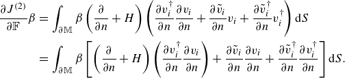 \begin{eqnarray} { \dfrac {\partial J^{(2)}}{\partial \mathbb {F}} \beta } &=& \int _{\partial \mathbb {M}} \beta \left ( \frac {\partial }{\partial n}+H \right ) \left ( \frac {\partial v_i^\dagger }{\partial n}\frac {\partial v_i}{\partial n} + \frac {\partial \tilde {v}_i}{\partial n} v_i + \frac {\partial \tilde {v}^{\dagger }_i}{\partial n} v_i^{\dagger } \right ) {\rm d}S \nonumber \\ &=& \int _{\partial \mathbb {M}} \beta \left [ \left ( \frac {\partial }{\partial n}+H \right ) \left ( \frac {\partial v_i^\dagger }{\partial n}\frac {\partial v_i}{\partial n} \right ) + \frac {\partial \tilde {v}_i}{\partial n}\frac {\partial v_i}{\partial n} + \frac {\partial \tilde {v}_i^\dagger }{\partial n}\frac {\partial v_i^\dagger }{\partial n} \right ] {\rm d}S. \end{eqnarray}
Therefore, one can identify from (2.36) the second-order shape sensitivity of $\bar {v}_i$
to a modification of the solid inclusion shape,
$\bar {v}_i$
to a modification of the solid inclusion shape,
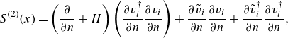 \begin{equation} S^{(2)}(x) = \left ( \frac {\partial }{\partial n}+H \right ) \left ( \frac {\partial v_i^\dagger }{\partial n}\frac {\partial v_i}{\partial n} \right ) + \frac {\partial \tilde {v}_i}{\partial n}\frac {\partial v_i}{\partial n} + \frac {\partial \tilde {v}_i^\dagger }{\partial n}\frac {\partial v_i^\dagger }{\partial n}, \end{equation}
which can be evaluated on $\partial \mathbb {M}$
once
$\partial \mathbb {M}$
once $v_i$
,
$v_i$
, $v_i^\dagger$
,
$v_i^\dagger$
, $\hat v_i$
and
$\hat v_i$
and $\hat v_i^\dagger$
have been computed by solving the direct and first- and second-order adjoint problems.
$\hat v_i^\dagger$
have been computed by solving the direct and first- and second-order adjoint problems.
3. Microscopic problems: comparison between direct and adjoint approaches
In this section, we compare the average values of the tensors $M_{ij}$
obtained by solving the direct microscopic problem (2.15) and evaluating (2.11) on the actual geometry with the prediction obtained by solving the adjoint microscopic problems (2.30), (2.40) and (2.42) on a reference geometry and evaluating (2.36). To simplify the analysis, we consider geometries for which relation (2.14) holds, i.e.
$M_{ij}$
obtained by solving the direct microscopic problem (2.15) and evaluating (2.11) on the actual geometry with the prediction obtained by solving the adjoint microscopic problems (2.30), (2.40) and (2.42) on a reference geometry and evaluating (2.36). To simplify the analysis, we consider geometries for which relation (2.14) holds, i.e. $\bar {N}_{ij}=-\bar {M}_{ij}$
. Details about the numerical solution are given in appendix C. As a test case, we use a REV containing two circular solid inclusions of different radii
$\bar {N}_{ij}=-\bar {M}_{ij}$
. Details about the numerical solution are given in appendix C. As a test case, we use a REV containing two circular solid inclusions of different radii $R_A$
and
$R_A$
and $R_B$
, depicted in figure 3(
$R_B$
, depicted in figure 3( $a$
).
$a$
).
This means that the considered membrane exhibits a periodicity for every two inclusions. We consider two families of small amplitude geometry modifications: a change in the radius of a solid inclusion (without displacing its centre, cf. figure 3 $b$
) and a displacement of the centre of one inclusion (without changing its shape, cf. figure 3
$b$
) and a displacement of the centre of one inclusion (without changing its shape, cf. figure 3 $c$
). In the following, we leave the compact notation introduced in (2.15) to analyse the direct and adjoint fields component by component. According to the notation introduced in (2.10) and the relations thoroughly explained in appendix B,
$c$
). In the following, we leave the compact notation introduced in (2.15) to analyse the direct and adjoint fields component by component. According to the notation introduced in (2.10) and the relations thoroughly explained in appendix B, $M_{ij}^{\dagger }$
,
$M_{ij}^{\dagger }$
, $\tilde {M}_{ij}$
and
$\tilde {M}_{ij}$
and $\tilde {M}_{ij}^{\dagger }$
denote the first, second, and third adjoint variables whose associated problems are (2.30), (2.40) and (2.42), respectively.
$\tilde {M}_{ij}^{\dagger }$
denote the first, second, and third adjoint variables whose associated problems are (2.30), (2.40) and (2.42), respectively.
( $a$
) Sketch of a REV containing two circular inclusions with centres in
$a$
) Sketch of a REV containing two circular inclusions with centres in $(x_n^A,x_t^A)=(0,0.2)$
,
$(x_n^A,x_t^A)=(0,0.2)$
, $(x_n^B,x_t^B)=(0,-0.2)$
and radii
$(x_n^B,x_t^B)=(0,-0.2)$
and radii $R_A=0.12$
and
$R_A=0.12$
and $R_B=0.15$
. We consider two cases for the deformation of the boundary of the inclusions
$R_B=0.15$
. We consider two cases for the deformation of the boundary of the inclusions $\partial \mathbb {M}$
: (
$\partial \mathbb {M}$
: ( $b$
) a purely normal deformation, consisting of a modification of the radius of the upper circular solid inclusion of a quantity
$b$
) a purely normal deformation, consisting of a modification of the radius of the upper circular solid inclusion of a quantity $\beta =\Delta R_A$
and
$\beta =\Delta R_A$
and $(c)$
an alteration
$(c)$
an alteration $\varDelta$
of the position
$\varDelta$
of the position $(x_t^A,0)$
of its centre. In both cases, the red arrows showing the deformation are directed along the normal to the original boundary (black solid line) and their length is proportional to
$(x_t^A,0)$
of its centre. In both cases, the red arrows showing the deformation are directed along the normal to the original boundary (black solid line) and their length is proportional to $\beta$
. The black dashes in (
$\beta$
. The black dashes in ( $b$
) and (
$b$
) and ( $c$
) represent the deformed boundary.
$c$
) represent the deformed boundary. $\theta \in [0,2\pi ]$
in panel
$\theta \in [0,2\pi ]$
in panel $(b)$
is an angular coordinate that spans the inclusion’s surface from the positive
$(b)$
is an angular coordinate that spans the inclusion’s surface from the positive $x_n$
, anticlockwise. This coordinate is used to plot the sensitivities
$x_n$
, anticlockwise. This coordinate is used to plot the sensitivities $S^{(1)}, S^{(2)}$
and the magnitude of the normal deformation
$S^{(1)}, S^{(2)}$
and the magnitude of the normal deformation $\beta$
along
$\beta$
along $\partial \mathbb {M}$
.
$\partial \mathbb {M}$
.
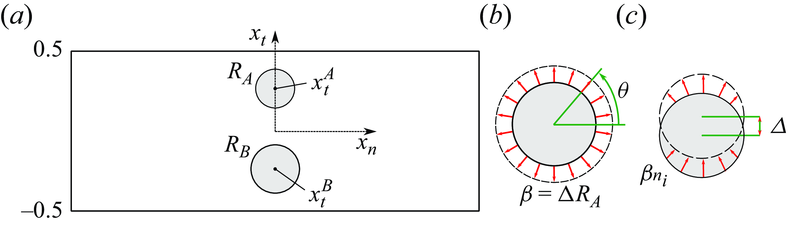
Solution of the ( $a,e$
) direct microscopic problems and (
$a,e$
) direct microscopic problems and ( $b$
–
$b$
– $d$
,
$d$
, $f$
–
$f$
– $h$
) adjoint microscopic problems in the geometric configuration shown in figure 3 with
$h$
) adjoint microscopic problems in the geometric configuration shown in figure 3 with $R_A=0.12, R_B=0.15, x_t^A=0.2$
and
$R_A=0.12, R_B=0.15, x_t^A=0.2$
and $ x_t^B=-0.2$
. Contour of magnitude
$ x_t^B=-0.2$
. Contour of magnitude $\sqrt {M_{n \cdot }^2+M_{t \cdot }^2}$
and streamlines (red) for the fields (
$\sqrt {M_{n \cdot }^2+M_{t \cdot }^2}$
and streamlines (red) for the fields ( $a$
)
$a$
) $(M_{nn},M_{tn})$
, (
$(M_{nn},M_{tn})$
, ( $b$
)
$b$
) $(M_{nn}^{\dagger },M_{tn}^{\dagger })$
, (
$(M_{nn}^{\dagger },M_{tn}^{\dagger })$
, ( $c$
)
$c$
) $(\tilde {M}_{nn},\tilde {M}_{tn})$
, (
$(\tilde {M}_{nn},\tilde {M}_{tn})$
, ( $d$
)
$d$
) $(\tilde {M}_{nn}^{\dagger },\tilde {M}_{tn}^{\dagger })$
, (
$(\tilde {M}_{nn}^{\dagger },\tilde {M}_{tn}^{\dagger })$
, ( $e$
)
$e$
) $(M_{nt},M_{tt})$
, (
$(M_{nt},M_{tt})$
, ( $f$
)
$f$
) $(M_{nt}^{\dagger },M_{tt}^{\dagger })$
, (
$(M_{nt}^{\dagger },M_{tt}^{\dagger })$
, ( $g$
)
$g$
) $(\tilde {M}_{nt},\tilde {M}_{tt})$
, (
$(\tilde {M}_{nt},\tilde {M}_{tt})$
, ( $h$
)
$h$
) $(\tilde {M}_{nt}^{\dagger },\tilde {M}_{tt}^{\dagger })$
are shown.
$(\tilde {M}_{nt}^{\dagger },\tilde {M}_{tt}^{\dagger })$
are shown.
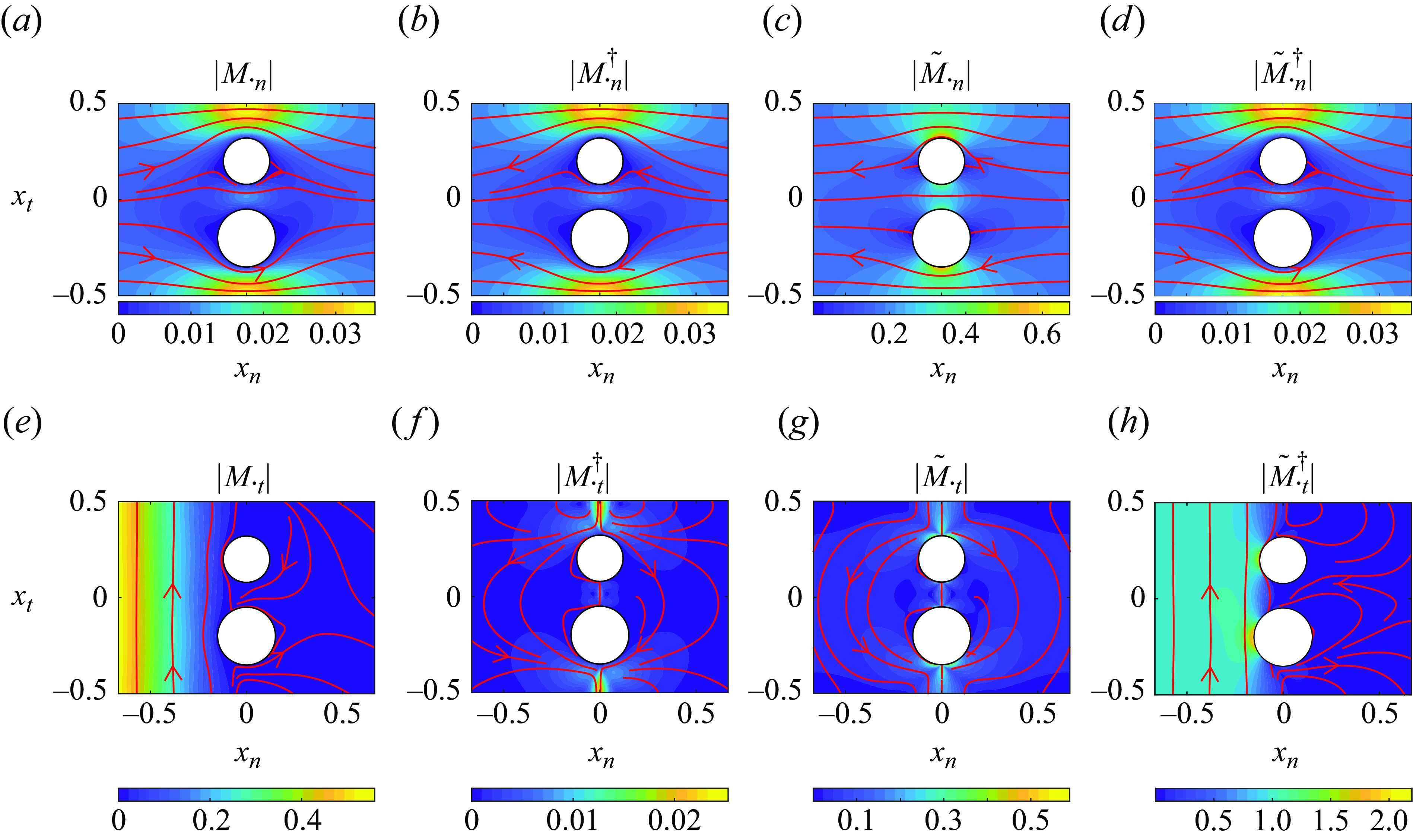
Figure 4 shows the contours and streamlines (red) of $M_{ij}$
(
$M_{ij}$
( $a,e$
),
$a,e$
), $M_{ij}^{\dagger }$
(
$M_{ij}^{\dagger }$
( $b,f$
),
$b,f$
), $\tilde {M}_{ij}$
(
$\tilde {M}_{ij}$
( $c,g$
) and
$c,g$
) and $\tilde {M}_{ij}^{\dagger }$
(
$\tilde {M}_{ij}^{\dagger }$
( $d,h$
) in the 2-D domain described in figure 3(
$d,h$
) in the 2-D domain described in figure 3( $a$
) with
$a$
) with $R_A=0.12, R_B=0.15, x_t^A=0.2$
and
$R_A=0.12, R_B=0.15, x_t^A=0.2$
and $ x_t^B=-0.2$
. Figure 4(
$ x_t^B=-0.2$
. Figure 4( $a,\!e$
) are obtained by computing (2.15), i.e. the direct problem. Figure 4(
$a,\!e$
) are obtained by computing (2.15), i.e. the direct problem. Figure 4( $b,\!f$
) are solutions of (2.30) for
$b,\!f$
) are solutions of (2.30) for $r_i=(1,0)$
and
$r_i=(1,0)$
and $(0,1)$
, respectively. These two fields do not depend on the direct solution, but only on
$(0,1)$
, respectively. These two fields do not depend on the direct solution, but only on $r_i$
. They can be computed once and for all for
$r_i$
. They can be computed once and for all for $\bar {M}_{ij}$
and the solution for the
$\bar {M}_{ij}$
and the solution for the $\bar {N}_{ij}$
fields is the same. Figure 4(
$\bar {N}_{ij}$
fields is the same. Figure 4( $c,\!g$
) are obtained by computing (2.40), which depend only on the solution of (2.30) by means of the inhomogeneous boundary condition on
$c,\!g$
) are obtained by computing (2.40), which depend only on the solution of (2.30) by means of the inhomogeneous boundary condition on $\partial \mathbb {M}$
. Figure 4(
$\partial \mathbb {M}$
. Figure 4( $d,\!h$
) are obtained by computing (2.42), which depend only on the direct solution through the inhomogeneous boundary condition on
$d,\!h$
) are obtained by computing (2.42), which depend only on the direct solution through the inhomogeneous boundary condition on $\partial \mathbb {M}$
. We now use these quantities to predict variations in the Navier tensors induced by small amplitude shape modifications.
$\partial \mathbb {M}$
. We now use these quantities to predict variations in the Navier tensors induced by small amplitude shape modifications.
Effect of a modification of the radius of inclusion A on the Navier tensors representing the membrane microstructure macroscopically. Panels (a,d,g), (b,e,h) and (c,f,i) refer to a single Navier tensor component. The sensitivities for each Navier tensor are shown in (a,d), (b,e) and (c,f). Each colour except black refers to one reference geometry used to compute these sensitivities. Reference geometry: $x_t^A=0.2$
,
$x_t^A=0.2$
, $x_t^B=-0.2$
,
$x_t^B=-0.2$
, $R_A=[0.054,0.120,0.186]$
(corresponding to red, green and blue) and
$R_A=[0.054,0.120,0.186]$
(corresponding to red, green and blue) and $R_B=0.15$
(cf. figure 3
$R_B=0.15$
(cf. figure 3 $a$
).
$a$
). $(a$
–
$(a$
– $c)$
First-order and
$c)$
First-order and $(d$
–
$(d$
– $f)$
second-order sensitivities of
$f)$
second-order sensitivities of $\bar {M}_{nn}$
,
$\bar {M}_{nn}$
, $\bar {M}_{nt}$
and
$\bar {M}_{nt}$
and $\bar {M}_{tt}$
on the boundary of inclusion A.
$\bar {M}_{tt}$
on the boundary of inclusion A. $(g$
-
$(g$
- $i)$
Here
$i)$
Here $\bar {M}_{nn}$
,
$\bar {M}_{nn}$
, $\bar {M}_{nt}$
and
$\bar {M}_{nt}$
and $\bar {M}_{tt}$
recomputed with the modified geometry (black solid line) and predicted from first-order (dashes) and second-order (dots) shape sensitivities. Coloured squares represent evaluation points of the sensitivities. Since
$\bar {M}_{tt}$
recomputed with the modified geometry (black solid line) and predicted from first-order (dashes) and second-order (dots) shape sensitivities. Coloured squares represent evaluation points of the sensitivities. Since $M_{tn}$
is antisymmetric with respect to the
$M_{tn}$
is antisymmetric with respect to the $x_n$
axis, its average
$x_n$
axis, its average $\bar {M}_{tn}$
is zero and
$\bar {M}_{tn}$
is zero and $\bar {N}_{ij}=-\bar {M}_{ij}$
.
$\bar {N}_{ij}=-\bar {M}_{ij}$
.
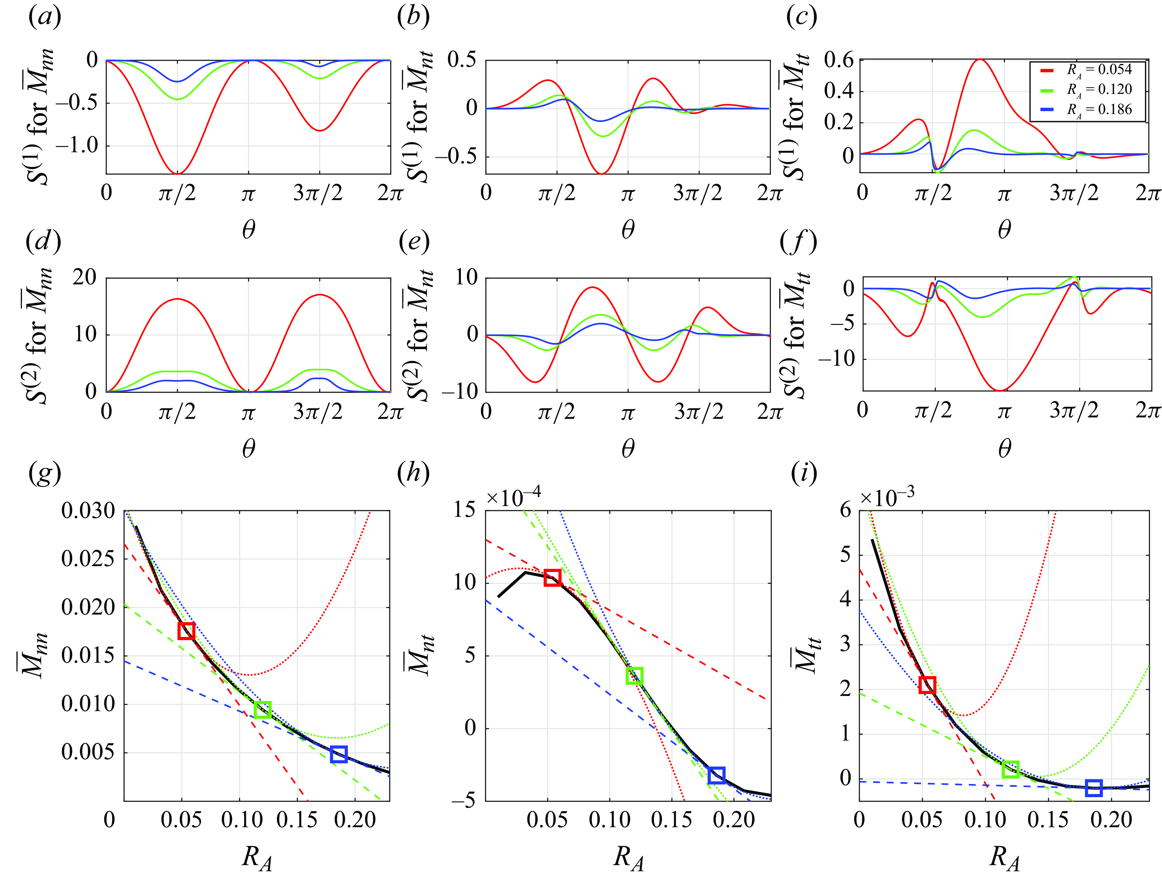
3.1. Radial shape perturbations of a circular solid inclusion
We let the radius $R_A$
of inclusion A vary while keeping the radius of inclusion B constant. Figure 5(
$R_A$
of inclusion A vary while keeping the radius of inclusion B constant. Figure 5( $a$
–
$a$
– $f$
) shows the first and second-order sensitivities of the different tensor components evaluated on three different reference geometries with
$f$
) shows the first and second-order sensitivities of the different tensor components evaluated on three different reference geometries with $R_A=0.054$
(red),
$R_A=0.054$
(red), $0.120$
(green) or
$0.120$
(green) or $0.186$
(blue). In this section, we modify the radius
$0.186$
(blue). In this section, we modify the radius $R_A$
only, which means that the normal deformation
$R_A$
only, which means that the normal deformation $\beta$
of the solid boundary
$\beta$
of the solid boundary $\partial \mathbb {M}$
is constant with
$\partial \mathbb {M}$
is constant with $\theta$
. We notice in figure 5(
$\theta$
. We notice in figure 5( $a,\!d$
) that the maxima (in absolute value) of
$a,\!d$
) that the maxima (in absolute value) of $\bar {M}_{nn}$
shape sensitivity are attained in
$\bar {M}_{nn}$
shape sensitivity are attained in $\theta =\pi /2$
and
$\theta =\pi /2$
and $\theta =3\pi /2$
or in a neighbourhood of these values. We saw in § 2.1.4 that
$\theta =3\pi /2$
or in a neighbourhood of these values. We saw in § 2.1.4 that $\bar {M}_{nn}$
has the physical meaning of a permeability coefficient. Now we can conclude that the membrane permeability is more sensitive to geometry changes in the pore between inclusions A and B (i.e. for example between the bottom part of inclusion A and the top part of inclusion B in figure 3
$\bar {M}_{nn}$
has the physical meaning of a permeability coefficient. Now we can conclude that the membrane permeability is more sensitive to geometry changes in the pore between inclusions A and B (i.e. for example between the bottom part of inclusion A and the top part of inclusion B in figure 3 $a$
) than on the upward or downward sides of the inclusion (i.e. their rightmost and leftmost portions in figure 3
$a$
) than on the upward or downward sides of the inclusion (i.e. their rightmost and leftmost portions in figure 3 $a$
). This is visually confirmed (note the adjacency of yellow and blue zone) in figure 4(
$a$
). This is visually confirmed (note the adjacency of yellow and blue zone) in figure 4( $a$
–
$a$
– $d$
), where the direct and adjoint fields all show steeper wall-normal gradients (which are quantities determining the sensitivities) in
$d$
), where the direct and adjoint fields all show steeper wall-normal gradients (which are quantities determining the sensitivities) in $\theta =\pi /2$
and
$\theta =\pi /2$
and $3\pi /2$
than in
$3\pi /2$
than in $\theta =0$
and
$\theta =0$
and $\pi$
, for example. The opposite stands for
$\pi$
, for example. The opposite stands for $\bar {M}_{tt}$
(figure 5
$\bar {M}_{tt}$
(figure 5 $c,\!f$
), whose shape sensitivity has a maximum in
$c,\!f$
), whose shape sensitivity has a maximum in $\theta =\pi$
, corresponding to the side of the solid inclusion facing the tangential boundary stress. On the other side (
$\theta =\pi$
, corresponding to the side of the solid inclusion facing the tangential boundary stress. On the other side ( $\theta =0$
), the sensitivity is close to zero, as wall-normal derivatives of the direct and adjoint fields are negligible (figure 4
$\theta =0$
), the sensitivity is close to zero, as wall-normal derivatives of the direct and adjoint fields are negligible (figure 4 $e$
–
$e$
– $h$
). We conclude that the slip coefficient is more sensitive to shape modifications of the upward or downward sides of the membrane than to its pore shapes. A mixed situation is found in the case of normally directed flow caused by tangential stress (
$h$
). We conclude that the slip coefficient is more sensitive to shape modifications of the upward or downward sides of the membrane than to its pore shapes. A mixed situation is found in the case of normally directed flow caused by tangential stress ( $\bar {M}_{nt}$
, cf. figure 5
$\bar {M}_{nt}$
, cf. figure 5 $b,\!e$
) since the most relevant values of the shape sensitivities are found for
$b,\!e$
) since the most relevant values of the shape sensitivities are found for $\theta$
near odd multiples of
$\theta$
near odd multiples of $\pi /4$
. The sensitivity maps in this case suggest that, if a larger
$\pi /4$
. The sensitivity maps in this case suggest that, if a larger $\bar {M}_{nt}$
is desired, one should ‘pull-and-push’ the solid boundary at alternating odd multiples of
$\bar {M}_{nt}$
is desired, one should ‘pull-and-push’ the solid boundary at alternating odd multiples of $\pi /4$
, creating a solid geometry that is asymmetric about the
$\pi /4$
, creating a solid geometry that is asymmetric about the $x_n$
axis. In figure 5(
$x_n$
axis. In figure 5( $g$
–
$g$
– $i$
), we compare the curves representing the direct computations of the
$i$
), we compare the curves representing the direct computations of the $\bar {M}_{ij}$
components (black solid lines) with the predictions based on
$\bar {M}_{ij}$
components (black solid lines) with the predictions based on $S^{(1)}$
only (red, green and blue dashes) and with the predictions based on both
$S^{(1)}$
only (red, green and blue dashes) and with the predictions based on both $S^{(1)}$
and
$S^{(1)}$
and $S^{(2)}$
(red, green and blue dots). The reference geometries used for predicting each coloured curve correspond to the squares of the same colour. The dashed lines representing the first-order predictions are tangent to the black solid line at the reference points (i.e. the squares), while the dotted parabolas have the same concavity as the solid black lines at the reference points.
$S^{(2)}$
(red, green and blue dots). The reference geometries used for predicting each coloured curve correspond to the squares of the same colour. The dashed lines representing the first-order predictions are tangent to the black solid line at the reference points (i.e. the squares), while the dotted parabolas have the same concavity as the solid black lines at the reference points.
The adjoint-based predictions and the direct evaluations of $\bar {M}_{ij}$
agree beyond the theoretical limit of infinitesimal deformations. In the presented cases, the worst second-order prediction corresponds to
$\bar {M}_{ij}$
agree beyond the theoretical limit of infinitesimal deformations. In the presented cases, the worst second-order prediction corresponds to $\bar {M}_{tt}$
for the reference radius
$\bar {M}_{tt}$
for the reference radius $R_A=0.054$
(red dots in figure 5
$R_A=0.054$
(red dots in figure 5 $i$
). For example, this prediction has a
$i$
). For example, this prediction has a $17.5\,\%$
error when
$17.5\,\%$
error when $R_A$
increases by
$R_A$
increases by $\sim 50\,\%$
to
$\sim 50\,\%$
to $0.075$
. If
$0.075$
. If $R_A$
is further increased, the error increases. The variation of
$R_A$
is further increased, the error increases. The variation of $\bar {M}_{tt}$
between the case with
$\bar {M}_{tt}$
between the case with $R_A=0.054$
and
$R_A=0.054$
and $R_A=0.075$
is approximately
$R_A=0.075$
is approximately $-32\,\%$
. The best case corresponds to
$-32\,\%$
. The best case corresponds to $\bar {M}_{nn}$
for a reference radius of
$\bar {M}_{nn}$
for a reference radius of $R_A=0.186$
(blue dots in figure 5
$R_A=0.186$
(blue dots in figure 5 $g$
), where the second-order prediction is in good agreement with the direct solutions in a range of deformations between
$g$
), where the second-order prediction is in good agreement with the direct solutions in a range of deformations between $-95\,\%$
and
$-95\,\%$
and $+24\,\%$
, with a maximum error of
$+24\,\%$
, with a maximum error of $\sim 11\,\%$
at
$\sim 11\,\%$
at $R_A=0.054$
(a
$R_A=0.054$
(a $-71\,\%$
deformation, corresponding to a
$-71\,\%$
deformation, corresponding to a $\sim 263\,\%$
variation in
$\sim 263\,\%$
variation in $\bar {M}_{nn}$
with respect to the reference case). In the considered cases, there always exists a range of
$\bar {M}_{nn}$
with respect to the reference case). In the considered cases, there always exists a range of $R_A$
in which second-order predictions are more accurate than first-order ones.
$R_A$
in which second-order predictions are more accurate than first-order ones.
Effect of a displacement $\varDelta$
of inclusion A along
$\varDelta$
of inclusion A along $x_t$
in terms in the Navier tensors representing the membrane microstructure macroscopically. First-order (black) and second-order (red) sensitivities of (
$x_t$
in terms in the Navier tensors representing the membrane microstructure macroscopically. First-order (black) and second-order (red) sensitivities of ( $a$
)
$a$
) $\bar {M}_{nn}$
, (
$\bar {M}_{nn}$
, ( $b$
)
$b$
) $\bar {M}_{nt}$
and (
$\bar {M}_{nt}$
and ( $c$
)
$c$
) $\bar {M}_{tt}$
on the boundary of inclusion A in the reference configuration
$\bar {M}_{tt}$
on the boundary of inclusion A in the reference configuration $x_t^A=0.218$
,
$x_t^A=0.218$
, $x_t^B=-0.2$
,
$x_t^B=-0.2$
, $R_A=0.125$
and
$R_A=0.125$
and $R_B=0.075$
(cf. figure 3
$R_B=0.075$
(cf. figure 3 $a$
), corresponding to the green square in panels
$a$
), corresponding to the green square in panels $(e{-}f)$
. (
$(e{-}f)$
. ( $d$
) Examples of normal deformation
$d$
) Examples of normal deformation $\beta$
induced by a displacement
$\beta$
induced by a displacement $\varDelta$
of inclusion A (colour legend) at each location
$\varDelta$
of inclusion A (colour legend) at each location $\theta$
along the solid inclusion.
$\theta$
along the solid inclusion. $(e$
–
$(e$
– $f)$
Here
$f)$
Here $\bar {M}_{nn}$
,
$\bar {M}_{nn}$
, $\bar {M}_{nt}$
and
$\bar {M}_{nt}$
and $\bar {M}_{tt}$
recomputed with the modified geometry (black solid line) and predicted from first-order (green dashes) and second-order (green dots) shape sensitivities. First-order (dashes) and second-order (dots) predictions for two additional reference locations
$\bar {M}_{tt}$
recomputed with the modified geometry (black solid line) and predicted from first-order (green dashes) and second-order (green dots) shape sensitivities. First-order (dashes) and second-order (dots) predictions for two additional reference locations $x_t^A$
are shown in red and blue. Coloured squares represent evaluation points of the sensitivities.
$x_t^A$
are shown in red and blue. Coloured squares represent evaluation points of the sensitivities.
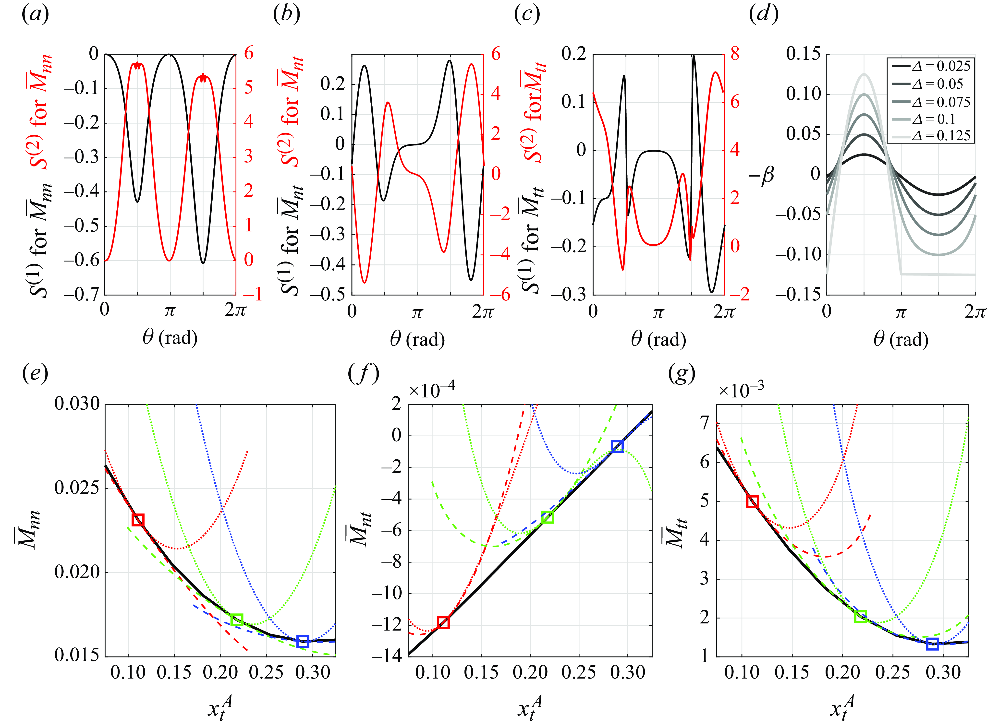
3.2. Displacement of the centre of a circular solid inclusion
In this section, we consider a more general deformation of the solid boundaries, obtained by shifting by a quantity $\varDelta$
(cf. figure 3
$\varDelta$
(cf. figure 3 $c$
) the position of the centre of a circular solid inclusion
$c$
) the position of the centre of a circular solid inclusion $x_t^A$
with respect to another, centred at
$x_t^A$
with respect to another, centred at $x_t^B$
(cf. figure 3). The geometry parameters for this configuration are
$x_t^B$
(cf. figure 3). The geometry parameters for this configuration are $R_A=0.125, R_B=0.075$
and
$R_A=0.125, R_B=0.075$
and $x_t^B=-0.2$
. Figure 6(
$x_t^B=-0.2$
. Figure 6( $a$
–
$a$
– $c$
) shows some distributions of sensitivity for the reference geometry with
$c$
) shows some distributions of sensitivity for the reference geometry with $x_t^A=0.218$
(green squares in figure 6
$x_t^A=0.218$
(green squares in figure 6 $e{-}g$
). A shift of the inclusion of a quantity
$e{-}g$
). A shift of the inclusion of a quantity $\varDelta$
causes a distribution of the normal deformation
$\varDelta$
causes a distribution of the normal deformation $\beta$
as shown in figure 6(
$\beta$
as shown in figure 6( $d$
). The local maxima (in absolute value) of
$d$
). The local maxima (in absolute value) of $\beta$
are located in
$\beta$
are located in $\theta =\pi /2,3\pi /2$
, except for
$\theta =\pi /2,3\pi /2$
, except for $\varDelta =R_A$
, where we observe a plateau in the range
$\varDelta =R_A$
, where we observe a plateau in the range $\theta \in [\pi ,2\pi ]$
. Indeed, when
$\theta \in [\pi ,2\pi ]$
. Indeed, when $\varDelta =R_A$
(lighter grey line corresponding to
$\varDelta =R_A$
(lighter grey line corresponding to $\varDelta =R_A=0.125$
), the image of half of the original inclusion reduces to a single point of the displaced inclusion. It is thus mathematically inconsistent to consider the case
$\varDelta =R_A=0.125$
), the image of half of the original inclusion reduces to a single point of the displaced inclusion. It is thus mathematically inconsistent to consider the case $\varDelta \gt R_A$
since some points of the original inclusion have no image on the displaced inclusion through a normal deformation. Note also that the function
$\varDelta \gt R_A$
since some points of the original inclusion have no image on the displaced inclusion through a normal deformation. Note also that the function $\beta$
in figure 6(
$\beta$
in figure 6( $d$
) passes by zero twice in its domain
$d$
) passes by zero twice in its domain $\theta \in (0,2\pi )$
. However, any displacement
$\theta \in (0,2\pi )$
. However, any displacement $\varDelta \neq 0$
of the centre causes all points on the circle to move of
$\varDelta \neq 0$
of the centre causes all points on the circle to move of $\varDelta$
. The existence of zeros in
$\varDelta$
. The existence of zeros in $\beta$
is a consequence of its definition as normal displacement. This means that there exist points which change position, but this movement has zero component along the normal to the reference geometry, thus
$\beta$
is a consequence of its definition as normal displacement. This means that there exist points which change position, but this movement has zero component along the normal to the reference geometry, thus $\beta =0$
in those points. In figure 6(
$\beta =0$
in those points. In figure 6( $e{-}g$
), we compare the actual (black line) and predicted value of
$e{-}g$
), we compare the actual (black line) and predicted value of $\bar {M}_{ij}$
with first-order (dashes) and second-order (dots) sensitivities computed using three base points (squares). Since
$\bar {M}_{ij}$
with first-order (dashes) and second-order (dots) sensitivities computed using three base points (squares). Since $\beta$
is not constant along
$\beta$
is not constant along $\partial \mathbb {M}$
, the first-order predictions are not lines and the second-order ones are not parabolas. The notion of slope and concavity used to assess the performance of the prediction in figure 5 cannot be used in this case and we can visually rely only on how close the predictions and the actual values are. We notice that we have a good agreement only for infinitesimal perturbations and most of the second-order predictions do not perform well for sensible deformations.
$\partial \mathbb {M}$
, the first-order predictions are not lines and the second-order ones are not parabolas. The notion of slope and concavity used to assess the performance of the prediction in figure 5 cannot be used in this case and we can visually rely only on how close the predictions and the actual values are. We notice that we have a good agreement only for infinitesimal perturbations and most of the second-order predictions do not perform well for sensible deformations.
In conclusion, displacements of $\partial \mathbb {M}$
having a strong tangential-to-the-reference-geometry component are more difficult to predict than those dominated by normal deformation. This condition is embedded in the hypothesis under which (2.20) is valid. However, for small displacements (i.e.
$\partial \mathbb {M}$
having a strong tangential-to-the-reference-geometry component are more difficult to predict than those dominated by normal deformation. This condition is embedded in the hypothesis under which (2.20) is valid. However, for small displacements (i.e. $\varDelta \ll R_A$
in this case), the first-order prediction can be trusted.
$\varDelta \ll R_A$
in this case), the first-order prediction can be trusted.
3.3. Application: efficient handling of parametric studies
In § 3.2, we considered a microscopic case constituted by a REV containing two solid inclusions. However, the adjoint procedure presented in this work does not depend on the choice of the REV. In the following section, we consider a REV containing a single solid inclusion. This geometrical configuration was used in Ledda et al. (Reference Ledda, Boujo, Camarri, Gallaire and Zampogna2021) to create a map of permeability and slip coefficients associated with a membrane formed by the periodic repetition of an elliptical solid inclusion. The map, obtained by interpolating a set of direct microscopic solutions, was used to optimise the flow around a porous thin membrane. Obtaining such a map involves a non-negligible computational cost.
Effect of a modification of the axis $l_n$
and
$l_n$
and $l_t$
of a single elliptic inclusion on the
$l_t$
of a single elliptic inclusion on the $\bar {M}_{ij}$
tensor (geometry shown in the insets of panel
$\bar {M}_{ij}$
tensor (geometry shown in the insets of panel $c$
). Reference geometry: circular solid inclusion (
$c$
). Reference geometry: circular solid inclusion ( $l_n=l_t=0.3$
; black stars in panels
$l_n=l_t=0.3$
; black stars in panels $c$
,
$c$
, $d$
) only.
$d$
) only. $(a)$
First-order (black) and second-order (red) shape sensitivities of
$(a)$
First-order (black) and second-order (red) shape sensitivities of $\bar {M}_{nn}$
(solid lines) and
$\bar {M}_{nn}$
(solid lines) and $\bar {M}_{tt}$
(dots) along
$\bar {M}_{tt}$
(dots) along $\partial \mathbb {M}$
as parametrised by
$\partial \mathbb {M}$
as parametrised by $\theta$
(cf. figure 3
$\theta$
(cf. figure 3 $b$
).
$b$
). $(b)$
Example of normal deformation
$(b)$
Example of normal deformation $\beta$
between the base circle with
$\beta$
between the base circle with $l_n=l_t=0.3$
and sample ellipses (
$l_n=l_t=0.3$
and sample ellipses ( $l_n,l_t$
in the legend).
$l_n,l_t$
in the legend). $(c,d)$
Contours of permeability
$(c,d)$
Contours of permeability $\bar {M}_{nn}$
and slip
$\bar {M}_{nn}$
and slip $\bar {M}_{tt}$
computed with a direct approach (solid lines) and with first-order (dashes) or second-order (dots) sensitivity.
$\bar {M}_{tt}$
computed with a direct approach (solid lines) and with first-order (dashes) or second-order (dots) sensitivity. $(e$
-
$(e$
- $h)$
Sample of the surfaces in
$h)$
Sample of the surfaces in $(c,d)$
at constant
$(c,d)$
at constant $l_t$
(
$l_t$
( $e,g$
) or
$e,g$
) or $l_n$
(
$l_n$
( $f,h$
). Colours correspond to ellipse semiaxes values as shown in the legend of each panel.
$f,h$
). Colours correspond to ellipse semiaxes values as shown in the legend of each panel.
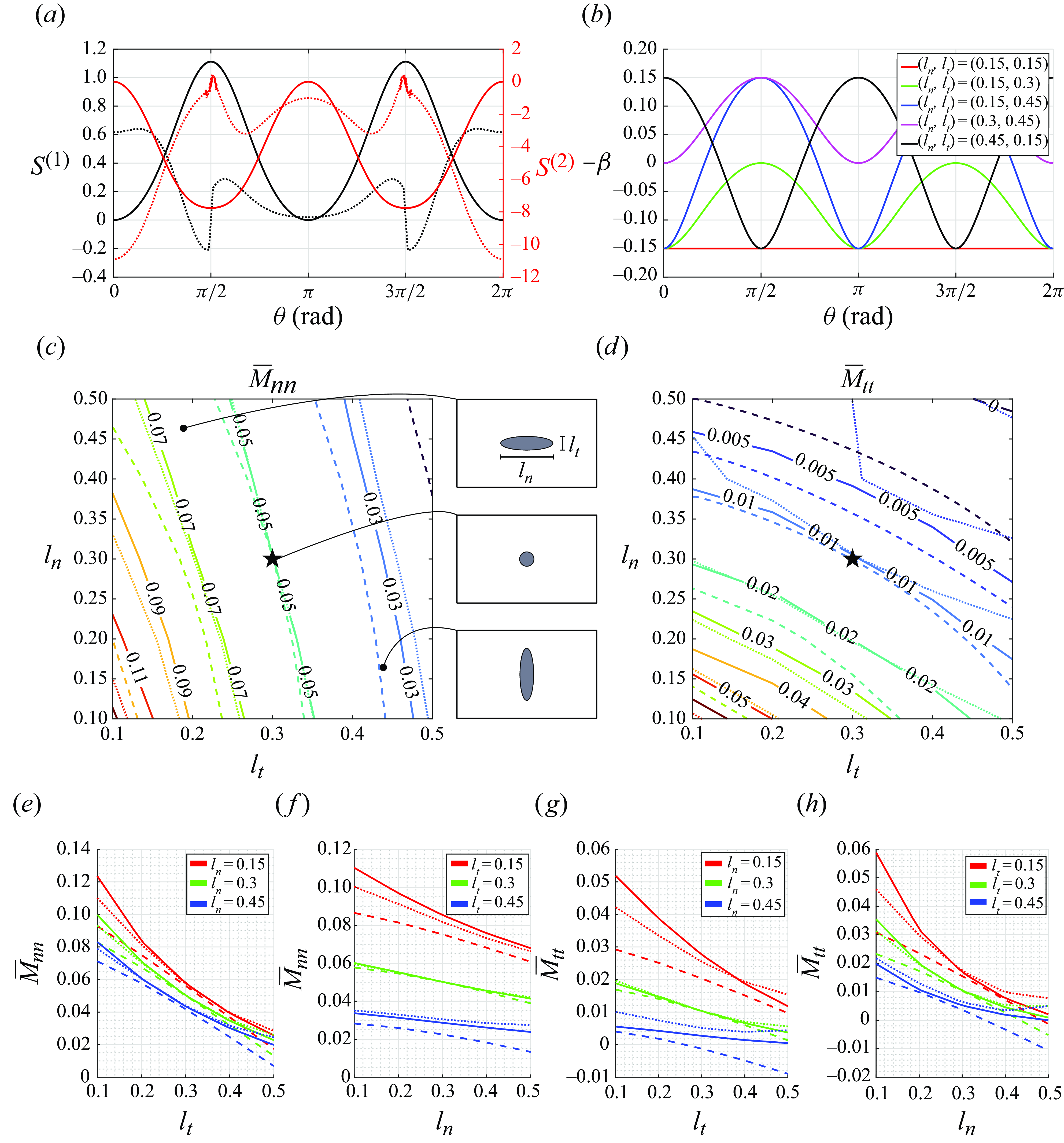
The objective of this section is to replicate a subset of the results obtained by Ledda et al. (Reference Ledda, Boujo, Camarri, Gallaire and Zampogna2021) using a single direct and adjoint microscopic solution. We consider an elliptic, isolated, solid inclusion of axes $l_n$
and
$l_n$
and $ l_t$
, aligned with the
$ l_t$
, aligned with the $(x_n, x_t)$
axes, respectively. We solve the direct microscopic problem around this geometry for a range of
$(x_n, x_t)$
axes, respectively. We solve the direct microscopic problem around this geometry for a range of $(l_n, l_t)$
values, obtaining the maps in solid line in figure 7(
$(l_n, l_t)$
values, obtaining the maps in solid line in figure 7( $c,\!d$
). We consider a base geometry for the adjoint computations constituted by a circle
$c,\!d$
). We consider a base geometry for the adjoint computations constituted by a circle $l_n=l_t=0.3$
(black star). The sensitivity distribution obtained in this configuration is shown in figure 7(
$l_n=l_t=0.3$
(black star). The sensitivity distribution obtained in this configuration is shown in figure 7( $a$
), while figure 7(
$a$
), while figure 7( $b$
) shows some distributions of the normal deformation
$b$
) shows some distributions of the normal deformation $\beta$
as a function of the ellipse semiaxes. Changes in permeability
$\beta$
as a function of the ellipse semiaxes. Changes in permeability $\bar {M}_{nn}$
or slip
$\bar {M}_{nn}$
or slip $\bar {M}_{tt}$
can be estimated via (2.36) with products involving the normal deformation beta and the sensitivities
$\bar {M}_{tt}$
can be estimated via (2.36) with products involving the normal deformation beta and the sensitivities $S^{(1)}$
and
$S^{(1)}$
and $S^{(2)}$
. These predictions of first order (dashes) and second order (dots) are plotted on the same isocontours obtained using the direct solutions for comparison (figure 7
$S^{(2)}$
. These predictions of first order (dashes) and second order (dots) are plotted on the same isocontours obtained using the direct solutions for comparison (figure 7 $c,\!d$
). There is a general agreement between the actual and predicted values of permeability and slip, confirmed also by the local sections of the maps, shown in figure 7(
$c,\!d$
). There is a general agreement between the actual and predicted values of permeability and slip, confirmed also by the local sections of the maps, shown in figure 7( $e$
–
$e$
– $h$
). Overall, second-order predictions improve over the first-order ones: in the
$h$
). Overall, second-order predictions improve over the first-order ones: in the $(l_n,l_t)$
space considered, the root mean square of the difference between the direct evaluation and the first- and second-order predictions are
$(l_n,l_t)$
space considered, the root mean square of the difference between the direct evaluation and the first- and second-order predictions are $(0.0084,0.0047)$
for
$(0.0084,0.0047)$
for $\bar {M}_{nn}$
and
$\bar {M}_{nn}$
and $(0.0078,0.0048)$
for
$(0.0078,0.0048)$
for $\bar {M}_{tt}$
, respectively. Local oscillations near
$\bar {M}_{tt}$
, respectively. Local oscillations near $\theta =\pi /2$
and
$\theta =\pi /2$
and $3\pi /2$
are due to numerical noise caused by the Dirac delta function. Their influence on the final solution is negligible, as shown in appendix C.
$3\pi /2$
are due to numerical noise caused by the Dirac delta function. Their influence on the final solution is negligible, as shown in appendix C.
We conclude that not only the method proposed in this paper is computationally lighter compared with the parametric study proposed in Ledda et al. (Reference Ledda, Boujo, Camarri, Gallaire and Zampogna2021), but also it allows for displacements of the solid boundaries of general shape. The numerical resolution has been carried out with the tools specified in appendix C. Using the same computer, the direct evaluation of $\bar {M}_{nn}$
and
$\bar {M}_{nn}$
and $\bar {M}_{tt}$
requires in this case approximately
$\bar {M}_{tt}$
requires in this case approximately $2.5$
hr with a step in
$2.5$
hr with a step in $l_n$
and
$l_n$
and $l_t$
of
$l_t$
of $0.02$
, whereas the sensitivity-based prediction takes approximately 6 min.
$0.02$
, whereas the sensitivity-based prediction takes approximately 6 min.
4. Comparison between macroscopic and full-scale solutions
In this section, we use the developed sensitivity-based procedure to predict the flow around a non-periodic porous membrane in a computationally efficient way. We compare full-scale solutions of the flow against macroscopic solutions (2.12) obtained by solving a microscopic problem for each solid inclusion and macroscopic solutions obtained by solving a single microscopic direct and adjoint problem and predicting the effect of the real geometry using shape sensitivities. We propose two complementary test cases: (i) the flow around and across a membrane whose solid inclusions are not periodic because of a small random perturbation and (ii) the flow across a membrane obstructing a channel, whose solid inclusions have a systematic deformation pattern, consisting of a linear variation of the inclusion radius. Notice that the macroscopic flows are normalised with the outer scales as in (2.4).
4.1. Membrane with random small perturbations of the solid inclusion
As a first test case, we consider a periodic 2-D membrane constituted by $20$
circles of radius
$20$
circles of radius $R=0.0125$
(i.e.
$R=0.0125$
(i.e. $\epsilon =0.05$
). The
$\epsilon =0.05$
). The $i$
th circle is centred at
$i$
th circle is centred at $(x_1^i,x_2^i)=(-\epsilon (i-0.5)/\sqrt {2},\epsilon (i-0.5)/\sqrt {2})$
. The membrane is placed in a vertical channel of size
$(x_1^i,x_2^i)=(-\epsilon (i-0.5)/\sqrt {2},\epsilon (i-0.5)/\sqrt {2})$
. The membrane is placed in a vertical channel of size $5\times 2$
. It is oriented at
$5\times 2$
. It is oriented at $45^{\circ }$
to the horizontal axis and traversed by a fluid flow which obeys Stokes equations (cf. sketch in figure 8). Dirichlet conditions
$45^{\circ }$
to the horizontal axis and traversed by a fluid flow which obeys Stokes equations (cf. sketch in figure 8). Dirichlet conditions $(u_1,u_2)=(0,1)$
apply on the bottom side and
$(u_1,u_2)=(0,1)$
apply on the bottom side and $u_i=0$
on the lateral sides and on the membrane solid inclusions. The Neumann condition
$u_i=0$
on the lateral sides and on the membrane solid inclusions. The Neumann condition $\Sigma _{ij}n_j=0$
applies on the top side. For convenience in the notation, we introduce a curvilinear coordinate
$\Sigma _{ij}n_j=0$
applies on the top side. For convenience in the notation, we introduce a curvilinear coordinate $\xi =\sqrt {x_1^2+x_2^2}$
, as shown in figure 8(
$\xi =\sqrt {x_1^2+x_2^2}$
, as shown in figure 8( $a$
). We radially perturb the surface of each solid inclusion using a Fourier series such that the
$a$
). We radially perturb the surface of each solid inclusion using a Fourier series such that the $i$
th deformed solid boundary has a radius
$i$
th deformed solid boundary has a radius
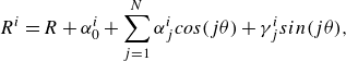 \begin{equation} R^i=R+\alpha _0^i+\sum _{j=1}^{N}\alpha _j^i cos(j\theta )+\gamma _j^i sin(j\theta ),\\ \end{equation}
where $\theta \in [0,2\pi ]$
,
$\theta \in [0,2\pi ]$
, $N=6$
and
$N=6$
and $\alpha _j^i,\gamma _j^i$
are randomly sampled coefficients from a uniform distribution in the range
$\alpha _j^i,\gamma _j^i$
are randomly sampled coefficients from a uniform distribution in the range $[-0.005\epsilon ,0.005\epsilon ]$
and collected in the Supplementary material. These solid inclusions are visualised in figure 9 (black lines, as opposed to the green lines, representing the reference geometry) and the full-scale solution of system (2.1) is visualised in figure 8(
$[-0.005\epsilon ,0.005\epsilon ]$
and collected in the Supplementary material. These solid inclusions are visualised in figure 9 (black lines, as opposed to the green lines, representing the reference geometry) and the full-scale solution of system (2.1) is visualised in figure 8( $a$
).
$a$
).
Full-scale and macroscopic simulations around an aperiodic membrane. ( $a$
) Contours of velocity magnitude and streamlines (red) for the full-scale simulation. The centre of each solid inclusion (grey obstacles) is located at
$a$
) Contours of velocity magnitude and streamlines (red) for the full-scale simulation. The centre of each solid inclusion (grey obstacles) is located at $(x_1^i,x_2^i)=(-\epsilon (i-0.5)/\sqrt {2},\epsilon (i-0.5)/\sqrt {2})$
, thus at the curvilinear coordinate
$(x_1^i,x_2^i)=(-\epsilon (i-0.5)/\sqrt {2},\epsilon (i-0.5)/\sqrt {2})$
, thus at the curvilinear coordinate $\xi ^i=\sqrt {x_{1,i}^2+x_{2,i}^2}=(i-0.5)\epsilon$
along
$\xi ^i=\sqrt {x_{1,i}^2+x_{2,i}^2}=(i-0.5)\epsilon$
along $\mathbb {C}$
, while the inset shows the typical streamline pattern in the proximity of the solid inclusions. (
$\mathbb {C}$
, while the inset shows the typical streamline pattern in the proximity of the solid inclusions. ( $b$
) Macroscopic simulation with
$b$
) Macroscopic simulation with $\bar {M}_{ij}$
and
$\bar {M}_{ij}$
and $\bar {N}_{ij}$
computed using REVs containing only one inclusion and (
$\bar {N}_{ij}$
computed using REVs containing only one inclusion and ( $c$
) macroscopic simulation with
$c$
) macroscopic simulation with $\bar {M}_{ij}$
and
$\bar {M}_{ij}$
and $\bar {N}_{ij}$
predicted using the shape sensitivities computed around a circle of radius
$\bar {N}_{ij}$
predicted using the shape sensitivities computed around a circle of radius $0.25\epsilon$
and multiplying them for the
$0.25\epsilon$
and multiplying them for the $\beta$
describing the difference between the considered solid inclusion and the reference circular one. The fictitious interface representing the membrane in panels (
$\beta$
describing the difference between the considered solid inclusion and the reference circular one. The fictitious interface representing the membrane in panels ( $b$
) and (
$b$
) and ( $c$
) is denoted by the black dashes. The flow enters from the bottom of the domain with a unit velocity in the vertical direction. The lateral sides are no-slip walls and at the outlet (top boundary),
$c$
) is denoted by the black dashes. The flow enters from the bottom of the domain with a unit velocity in the vertical direction. The lateral sides are no-slip walls and at the outlet (top boundary), $\Sigma _{ij}n_j=0$
.
$\Sigma _{ij}n_j=0$
.
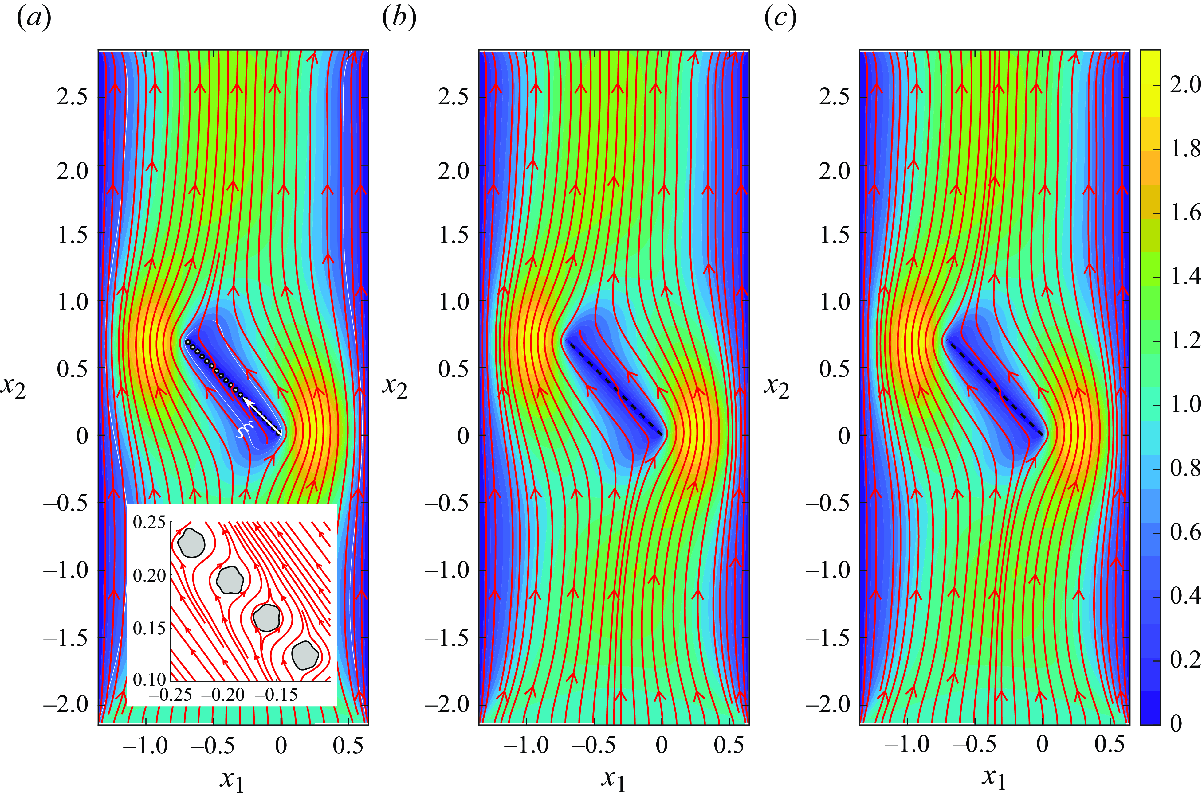
Details of the inclusions in the aperiodic membrane of figure 8. The boundaries of the original circular inclusions are sketched in dashed green line while the actual geometry is sketched in solid black line. Index $i$
increases from top to bottom and from left to right.
$i$
increases from top to bottom and from left to right.
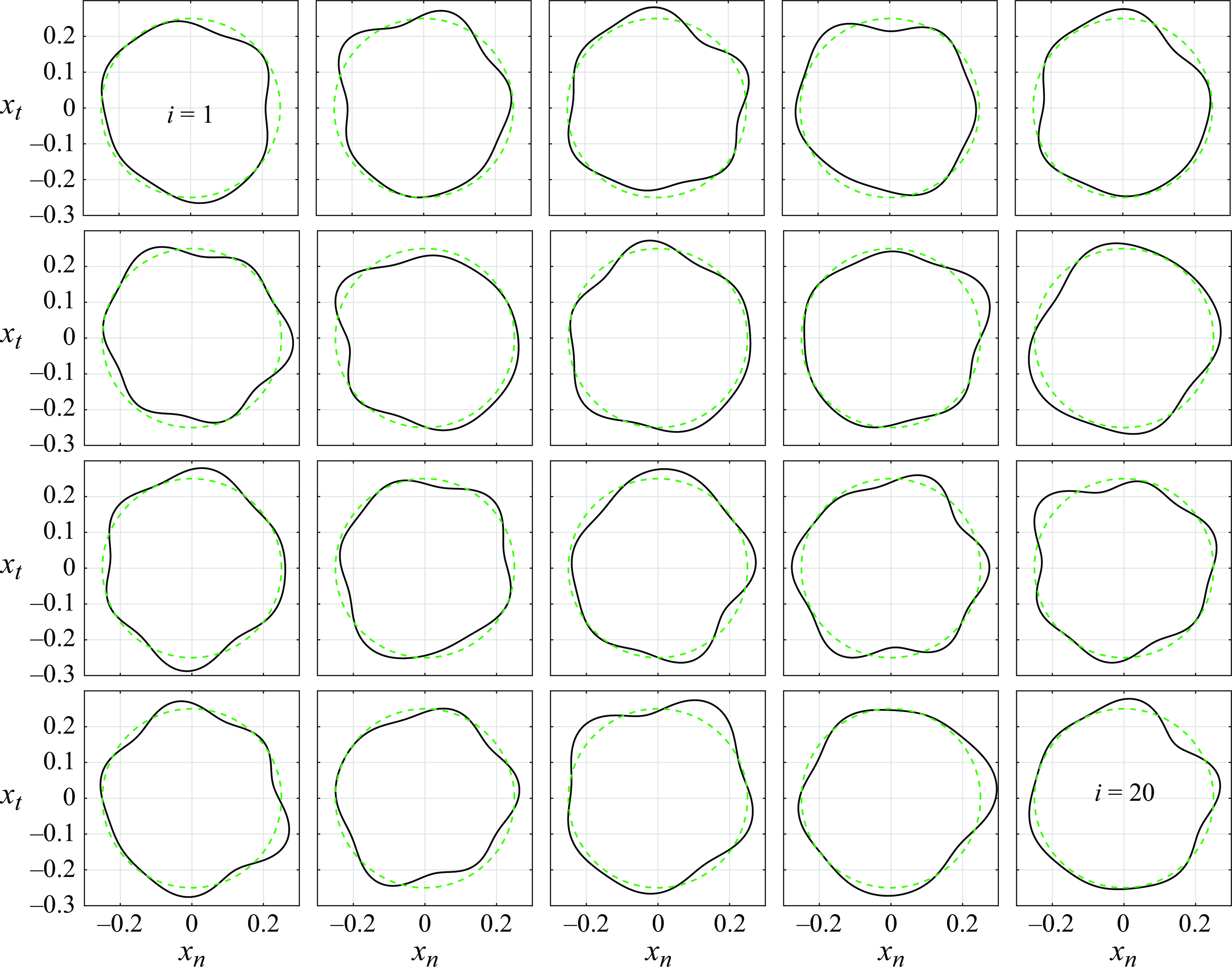
In the macroscopic simulation, we solve (2.5) with (2.12), which requires $\bar {M_{ij}}$
and
$\bar {M_{ij}}$
and $\bar {N}_{ij}$
. For the microscopic problems, we choose a REV containing a single solid inclusion at a time along the membrane (Ledda et al. Reference Ledda, Boujo, Camarri, Gallaire and Zampogna2021) and average one by one the microscopic direct problems on each of the
$\bar {N}_{ij}$
. For the microscopic problems, we choose a REV containing a single solid inclusion at a time along the membrane (Ledda et al. Reference Ledda, Boujo, Camarri, Gallaire and Zampogna2021) and average one by one the microscopic direct problems on each of the $20$
inclusion geometries. The tensors obtained in this case are used to compute the macroscopic fluid flow presented in figure 8(
$20$
inclusion geometries. The tensors obtained in this case are used to compute the macroscopic fluid flow presented in figure 8( $b$
). The computational cost of this operation is that of solving
$b$
). The computational cost of this operation is that of solving $80$
Stokes problems (2.15). Equivalently, this means solving
$80$
Stokes problems (2.15). Equivalently, this means solving $20$
times (one for each inclusion) (2.10), which contains two components for
$20$
times (one for each inclusion) (2.10), which contains two components for $M_{ij}$
and another two for
$M_{ij}$
and another two for $N_{ij}$
.
$N_{ij}$
.
We now consider the macroscopic solution obtained using the sensitivity-based workflow. To obtain $\bar {M}_{ij}$
and
$\bar {M}_{ij}$
and $\bar {N}_{ij}$
, we solve the direct problem (2.15) and adjoint problems (2.30, 2.40, 2.42) around a circular solid inclusion of radius
$\bar {N}_{ij}$
, we solve the direct problem (2.15) and adjoint problems (2.30, 2.40, 2.42) around a circular solid inclusion of radius $R$
, finding the shape sensitivities
$R$
, finding the shape sensitivities $S^{(1)}$
and
$S^{(1)}$
and $S^{(2)}$
for all
$S^{(2)}$
for all $\bar {M}_{ij}$
and
$\bar {M}_{ij}$
and $\bar {N}_{ij}$
components. We then evaluate (2.36) with the normal displacement
$\bar {N}_{ij}$
components. We then evaluate (2.36) with the normal displacement
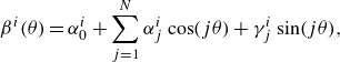 \begin{equation} \beta ^i(\theta )=\alpha _0^i+\sum _{j=1}^{N}\alpha _j^i \cos(j\theta )+\gamma _j^i \sin(j\theta ), \end{equation}
from the reference circular inclusion, obtaining an estimate for the variation of $\bar {M}_{ij}$
and
$\bar {M}_{ij}$
and $\bar {N}_{ij}$
caused by the shape modification. The computational cost of this operation is
$\bar {N}_{ij}$
caused by the shape modification. The computational cost of this operation is $12$
Stokes problems (i.e. four for the direct solution and two for the first adjoint problem to find
$12$
Stokes problems (i.e. four for the direct solution and two for the first adjoint problem to find $S^{(1)}$
and another six to find
$S^{(1)}$
and another six to find $S^{(2)}$
), regardless of the number of inclusions (and neglecting potential tensor symmetries, which would possibly reduce this cost). The macroscopic fluid flow obtained with these estimates is visualised in figure 8(
$S^{(2)}$
), regardless of the number of inclusions (and neglecting potential tensor symmetries, which would possibly reduce this cost). The macroscopic fluid flow obtained with these estimates is visualised in figure 8( $c$
) by means of streamlines and isocontours of velocity magnitude.
$c$
) by means of streamlines and isocontours of velocity magnitude.
Velocity and Navier tensors on the centreline $\mathbb {C}$
of the aperiodic membrane of figures 8 and 9. (
$\mathbb {C}$
of the aperiodic membrane of figures 8 and 9. ( $a$
) Normal- and (
$a$
) Normal- and ( $b$
) tangential-to-the-membrane velocity components. Black line, full-scale solution without averaging; black dots, averaged full-scale solution; blue line, macroscopic solution with
$b$
) tangential-to-the-membrane velocity components. Black line, full-scale solution without averaging; black dots, averaged full-scale solution; blue line, macroscopic solution with $\bar {M}_{ij}$
and
$\bar {M}_{ij}$
and $\bar {N}_{ij}$
computed cell-by-cell; red line, sensitivity-based predictions on the reference, undeformed geometry (circular inclusion). Additionally, the green line shows the macroscopic solution computed with undeformed circular inclusions, to highlight the differences caused by the geometry modification. Panels (
$\bar {N}_{ij}$
computed cell-by-cell; red line, sensitivity-based predictions on the reference, undeformed geometry (circular inclusion). Additionally, the green line shows the macroscopic solution computed with undeformed circular inclusions, to highlight the differences caused by the geometry modification. Panels ( $c$
–
$c$
– $j$
) show the tensors values along the membrane: (
$j$
) show the tensors values along the membrane: ( $c$
)
$c$
) $\bar {M}_{nn}$
, (
$\bar {M}_{nn}$
, ( $d$
)
$d$
) $\bar {M}_{nt}$
, (
$\bar {M}_{nt}$
, ( $e$
)
$e$
) $\bar {M}_{tn}$
, (
$\bar {M}_{tn}$
, ( $f$
)
$f$
) $\bar {M}_{tt}$
, (
$\bar {M}_{tt}$
, ( $g$
)
$g$
) $\bar {N}_{nn}$
, (
$\bar {N}_{nn}$
, ( $h$
)
$h$
) $\bar {N}_{nt}$
, (
$\bar {N}_{nt}$
, ( $i$
)
$i$
) $\bar {N}_{tn}$
, (
$\bar {N}_{tn}$
, ( $j$
)
$j$
) $\bar {N}_{tt}$
. Values directly computed via (2.15) are depicted in blue while the values predicted using shape sensitivities (2.36) are in red. The values associated with the reference circular geometry are in green.
$\bar {N}_{tt}$
. Values directly computed via (2.15) are depicted in blue while the values predicted using shape sensitivities (2.36) are in red. The values associated with the reference circular geometry are in green.
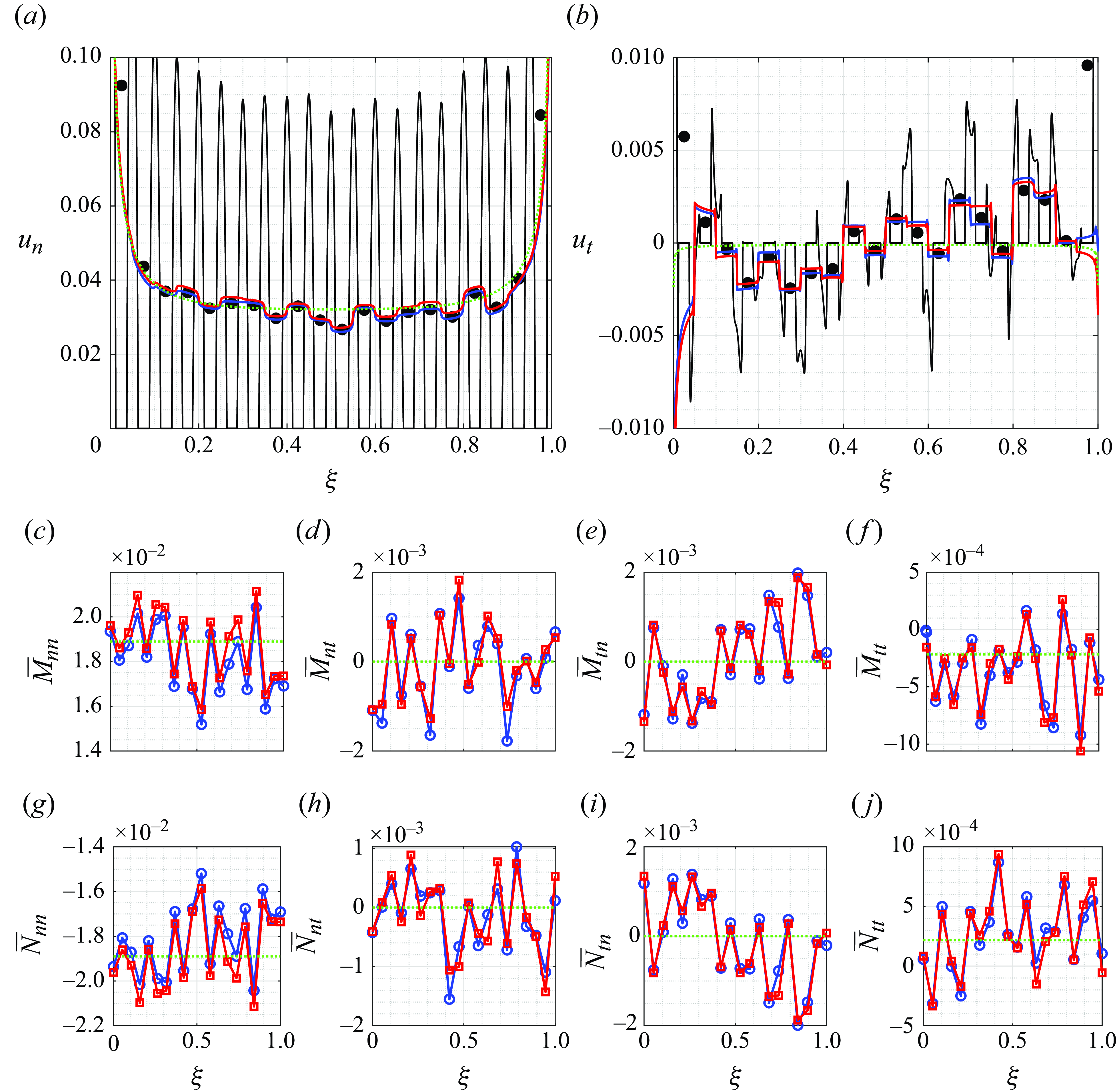
Figure 10( $a,\!b$
) compares the velocity profiles on the membrane centreline for the full-scale solution (black lines, average values as dots), direct macroscopic solution (blue) and shape sensitivity-based prediction (red). The agreement of both macroscopic solutions (direct and adjoint) with the average full-scale solution is excellent. For reference, green dots represent the macroscopic solution obtained by computing
$a,\!b$
) compares the velocity profiles on the membrane centreline for the full-scale solution (black lines, average values as dots), direct macroscopic solution (blue) and shape sensitivity-based prediction (red). The agreement of both macroscopic solutions (direct and adjoint) with the average full-scale solution is excellent. For reference, green dots represent the macroscopic solution obtained by computing $\bar {M}_{ij}$
and
$\bar {M}_{ij}$
and $\bar {N}_{ij}$
with the base (undeformed) circular inclusions. The values of the
$\bar {N}_{ij}$
with the base (undeformed) circular inclusions. The values of the $\bar {M}_{ij}$
and
$\bar {M}_{ij}$
and $\bar {N}_{ij}$
tensors computed using the direct (blue) and adjoint (red) procedures are shown in figure 10(
$\bar {N}_{ij}$
tensors computed using the direct (blue) and adjoint (red) procedures are shown in figure 10( $c$
–
$c$
– $j$
). Interestingly, although the geometric modifications may seem small (figure 9), the corresponding microscopic tensor values significantly vary. These variations cause peaks of tangential velocity, which are absent for the undeformed, circular inclusions. We can ascribe these differences entirely to the anisotropic nature of the deformed inclusions. The sensitivity-based prediction proves nearly as accurate as the direct solution, with a considerably lower computational cost. Indeed, the relative error on the membrane velocity magnitude with respect to the average full-scale solution (excluding the first and last REVs) is
$j$
). Interestingly, although the geometric modifications may seem small (figure 9), the corresponding microscopic tensor values significantly vary. These variations cause peaks of tangential velocity, which are absent for the undeformed, circular inclusions. We can ascribe these differences entirely to the anisotropic nature of the deformed inclusions. The sensitivity-based prediction proves nearly as accurate as the direct solution, with a considerably lower computational cost. Indeed, the relative error on the membrane velocity magnitude with respect to the average full-scale solution (excluding the first and last REVs) is $2.77\,\%$
for the macroscopic direct simulation and
$2.77\,\%$
for the macroscopic direct simulation and $2.90\,\%$
for the macroscopic adjoint-aided prediction, while the computational cost of the adjoint-aided simulation is approximately
$2.90\,\%$
for the macroscopic adjoint-aided prediction, while the computational cost of the adjoint-aided simulation is approximately $6.7$
times lower. In this section, we expressed the computational cost in terms of Stokes problems because the microscopic direct and adjoint problems are a set of Stokes problems which can be solved in a cascade. To translate this cost in computational time, consider that the computational time associated with a single Stokes solution is approximately 50 s on a laptop with 32 GB RAM and one INTEL i 9–10900HK CPU with eight cores.
$6.7$
times lower. In this section, we expressed the computational cost in terms of Stokes problems because the microscopic direct and adjoint problems are a set of Stokes problems which can be solved in a cascade. To translate this cost in computational time, consider that the computational time associated with a single Stokes solution is approximately 50 s on a laptop with 32 GB RAM and one INTEL i 9–10900HK CPU with eight cores.
4.2. Membrane with large systematic deformations of the solid inclusions
The developed procedure can handle small random geometry variations of the solid inclusions, resulting in membrane velocity profiles with random peaks. However, one may argue that the effect on the macroscopic flow of such modifications is captured – on average – by the green profile in figure 10( $a,\!b$
) (corresponding to a periodic membrane of base circles) and thus that the effect of these geometry modifications is not significant at the macroscale. We emphasise that the present method can capture macroscopic flow modifications. We consider the flow across a membrane constituted by
$a,\!b$
) (corresponding to a periodic membrane of base circles) and thus that the effect of these geometry modifications is not significant at the macroscale. We emphasise that the present method can capture macroscopic flow modifications. We consider the flow across a membrane constituted by $20$
inclusions of radii
$20$
inclusions of radii $R^i=0.2\epsilon ^2({i-1}/{1-\epsilon })+0.15\epsilon$
and evenly spaced centres. The average radius, used for the computation of the shape sensitivities is thus the same as in figure 9. The associated normal displacement of the solid boundary about the average radius reaches peak values of
$R^i=0.2\epsilon ^2({i-1}/{1-\epsilon })+0.15\epsilon$
and evenly spaced centres. The average radius, used for the computation of the shape sensitivities is thus the same as in figure 9. The associated normal displacement of the solid boundary about the average radius reaches peak values of $\pm 40\,\%$
at the membrane extremes. The so-constituted membrane obstructs a 2-D channel of unit height, as shown in figure 11(
$\pm 40\,\%$
at the membrane extremes. The so-constituted membrane obstructs a 2-D channel of unit height, as shown in figure 11( $a$
). The flow enters from the left-hand side of the domain horizontally with unit speed and exits from the right-hand side with zero stress, and the top and bottom sides are no-slip walls. Contrary to the previous case, where the fluid could flow around the membrane, it is now forced to flow across it. The fluid prefers to flow in the lower-half of the channel where the porosity of the membrane is larger. The flow is hence asymmetric about the centreline
$a$
). The flow enters from the left-hand side of the domain horizontally with unit speed and exits from the right-hand side with zero stress, and the top and bottom sides are no-slip walls. Contrary to the previous case, where the fluid could flow around the membrane, it is now forced to flow across it. The fluid prefers to flow in the lower-half of the channel where the porosity of the membrane is larger. The flow is hence asymmetric about the centreline $x_2=0.5$
. Similarly to the previous case, we compare the full-scale solution (figure 11
$x_2=0.5$
. Similarly to the previous case, we compare the full-scale solution (figure 11 $a$
) with a macroscopic solution of the flow past a membrane with all circular inclusions having the same radius
$a$
) with a macroscopic solution of the flow past a membrane with all circular inclusions having the same radius $0.25\epsilon$
(figure 11
$0.25\epsilon$
(figure 11 $b$
) and with space-varying microscopic geometry whose tensors are calculated using the direct (figure 11
$b$
) and with space-varying microscopic geometry whose tensors are calculated using the direct (figure 11 $c$
) and adjoint (figure 11
$c$
) and adjoint (figure 11 $d$
) approach. For the adjoint case, the sensitivity is calculated with a circular solid inclusion of radius
$d$
) approach. For the adjoint case, the sensitivity is calculated with a circular solid inclusion of radius $0.25\epsilon$
as reference geometry. The values of
$0.25\epsilon$
as reference geometry. The values of $\bar {M}_{nn}$
and
$\bar {M}_{nn}$
and $\bar {M}_{tt}$
used to compute the solutions in frames figure 11(
$\bar {M}_{tt}$
used to compute the solutions in frames figure 11( $b,\!c,\!d$
) are represented in figure 11(
$b,\!c,\!d$
) are represented in figure 11( $f,\!g$
) by green, blue and red lines, respectively.
$f,\!g$
) by green, blue and red lines, respectively.
Full-scale and macroscopic flow past an aperiodic membrane constituted by $20$
circular inclusions (i.e.
$20$
circular inclusions (i.e. $\epsilon =0.05$
). The radii linearly vary between
$\epsilon =0.05$
). The radii linearly vary between $0.15\epsilon$
(lowermost inclusion) and
$0.15\epsilon$
(lowermost inclusion) and $0.35\epsilon$
(uppermost inclusion). The centre of the
$0.35\epsilon$
(uppermost inclusion). The centre of the $n$
th inclusion is located in
$n$
th inclusion is located in $(x_1^n,x_2^n)=(0,(n-1/2)\epsilon )$
. In panels (
$(x_1^n,x_2^n)=(0,(n-1/2)\epsilon )$
. In panels ( $a{-}d$
) the contours of velocity magnitude and streamlines (red) are shown: (
$a{-}d$
) the contours of velocity magnitude and streamlines (red) are shown: ( $a$
) full-scale solution; (
$a$
) full-scale solution; ( $b$
) macroscopic solution past a periodic membrane formed by circular inclusions of radius
$b$
) macroscopic solution past a periodic membrane formed by circular inclusions of radius $0.25\epsilon$
; (
$0.25\epsilon$
; ( $c$
) macroscopic solution with
$c$
) macroscopic solution with $\bar {M}_{ij}$
and
$\bar {M}_{ij}$
and $\bar {N}_{ij}$
computed using REVs containing only one inclusion; (
$\bar {N}_{ij}$
computed using REVs containing only one inclusion; ( $d$
) macroscopic solution with
$d$
) macroscopic solution with $\bar {M}_{ij}$
and
$\bar {M}_{ij}$
and $\bar {N}_{ij}$
predicted using the shape sensitivities computed around a circular inclusion of radius
$\bar {N}_{ij}$
predicted using the shape sensitivities computed around a circular inclusion of radius $0.25\epsilon$
. The fictitious interface representing the membrane in panels (
$0.25\epsilon$
. The fictitious interface representing the membrane in panels ( $b,c$
) and (
$b,c$
) and ( $d$
) is denoted by the black dashes. The flow enters from the left of the domain with a unit velocity in the horizontal direction. The top and bottom of the panels are no-slip walls and at the outlet
$d$
) is denoted by the black dashes. The flow enters from the left of the domain with a unit velocity in the horizontal direction. The top and bottom of the panels are no-slip walls and at the outlet $\Sigma _{ij}n_j=0$
. (
$\Sigma _{ij}n_j=0$
. ( $e$
) Velocity magnitude at the membrane centreline (colour code as in figure 10
$e$
) Velocity magnitude at the membrane centreline (colour code as in figure 10 $a,\!b$
). (
$a,\!b$
). ( $f,g$
) Non-zero
$f,g$
) Non-zero $\bar {M}_{ij}$
components along the membrane (colour code as in figure 10
$\bar {M}_{ij}$
components along the membrane (colour code as in figure 10 $c{-}j$
). By symmetry,
$c{-}j$
). By symmetry, $\bar {N}_{ij}=-\bar {M}_{ij}$
and
$\bar {N}_{ij}=-\bar {M}_{ij}$
and $\bar {M}_{ij}=0$
if
$\bar {M}_{ij}=0$
if $i\neq j$
.
$i\neq j$
.
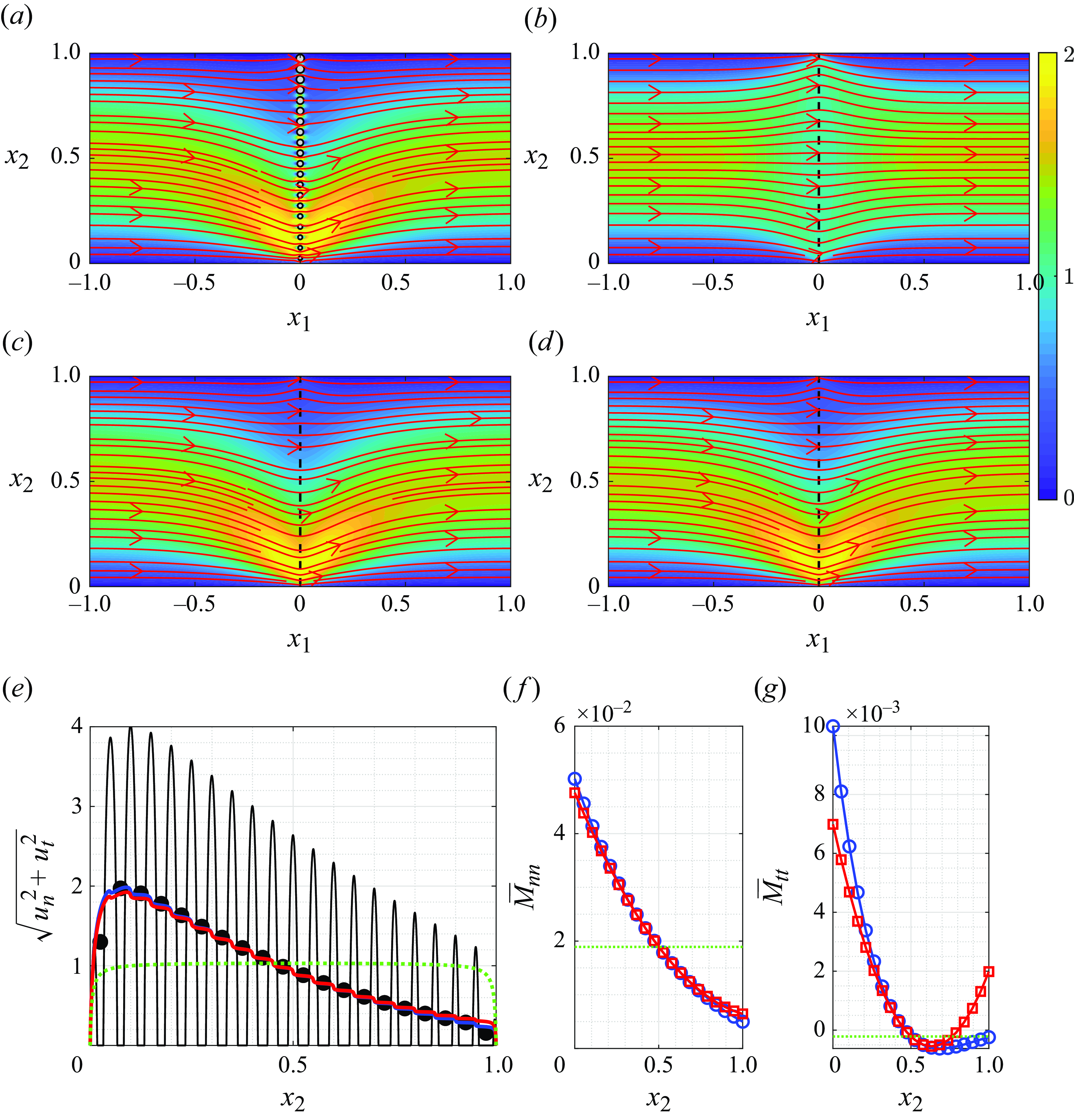
The velocity magnitude contours between the full-scale (figure 11 $a$
), macroscopic direct (
$a$
), macroscopic direct ( $c$
) and sensitivity-based (
$c$
) and sensitivity-based ( $d$
) simulations are in good agreement. The differences with respect to the flow through a periodic, unperturbed membrane (cf. figure 11
$d$
) simulations are in good agreement. The differences with respect to the flow through a periodic, unperturbed membrane (cf. figure 11 $b$
, where the flow is symmetric with respect to the
$b$
, where the flow is symmetric with respect to the $x_2=0.5$
axis) are important. This is confirmed by the velocity magnitude profiles along the membrane (figure 11
$x_2=0.5$
axis) are important. This is confirmed by the velocity magnitude profiles along the membrane (figure 11 $e$
), where we adopted the same colour code as in figure 10(
$e$
), where we adopted the same colour code as in figure 10( $a,\!b$
). The green line is indeed symmetric about
$a,\!b$
). The green line is indeed symmetric about $x_2=0.5$
, while the full-scale flow is not. As in the previous flow configuration, the full-scale average fields are correctly predicted both in the direct and sensitivity-based simulations, with minor differences, and at a much-reduced cost for the latter.
$x_2=0.5$
, while the full-scale flow is not. As in the previous flow configuration, the full-scale average fields are correctly predicted both in the direct and sensitivity-based simulations, with minor differences, and at a much-reduced cost for the latter.
The two examples presented in this section show complementary applications of the proposed model: in the former, the fluid can flow around the membrane and the random geometry modifications locally change the flow along the membrane, while in the latter, the membrane obstructs a channel, forcing the flow through its pores, whose geometric properties globally alter the macroscopic flow. The present model handles both cases, offering an advantageous trade-off between accuracy and computational cost.
5. Conclusions
In the present paper, we considered the problem of computing the fluid flow across a thin, aperiodic porous membrane in an efficient way, coupling the homogenisation technique developed by Zampogna & Gallaire (Reference Zampogna and Gallaire2020) with a second-order shape-sensitivity approach. We introduced the concept of REV in the model developed in Zampogna & Gallaire (Reference Zampogna and Gallaire2020) to account for the aperiodic porous microstructure. Using the separation of scales between the pore- and membrane-level flows, we wrote the macroscopic velocity field on the membrane as a linear combination of the stresses acting on the two sides of the membrane itself. The coefficients of the linear combination, the Navier tensors $\bar {M}_{ij}$
and
$\bar {M}_{ij}$
and $\bar {N}_{ij}$
, stem from the solution of solvability conditions at the REV scale, the microscopic problems, after an averaging step. While
$\bar {N}_{ij}$
, stem from the solution of solvability conditions at the REV scale, the microscopic problems, after an averaging step. While $\bar {M}_{ij}$
and
$\bar {M}_{ij}$
and $\bar {N}_{ij}$
only need to be computed once for a periodic microstructure, this is not possible for aperiodic geometries. Indeed, several direct microscopic solutions are needed only to find the proper REV size. The cost of this direct tensor evaluation scales with the number of pores/inclusions and quickly annihilates the computational gain of the homogeneous, macroscopic model.
$\bar {N}_{ij}$
only need to be computed once for a periodic microstructure, this is not possible for aperiodic geometries. Indeed, several direct microscopic solutions are needed only to find the proper REV size. The cost of this direct tensor evaluation scales with the number of pores/inclusions and quickly annihilates the computational gain of the homogeneous, macroscopic model.
Consequently, we developed an adjoint-based technique to account for geometrical modifications of the pore-scale microstructure starting from some reference geometry and in the limit of infinitesimal deformations. The computational cost of such an operation is constant with respect to the number of pores/inclusions, only requiring a small set of linear problems to be solved at the pore scale, the adjoint problems. We validated this procedure against direct solutions of the microscopic problems and found that it can predict the effect of moderately small geometric perturbations of the solid inclusions. To conclude our analysis, we considered a full-scale membrane of randomly perturbed microstructure and a membrane of circular inclusions of linearly increasing radius. We compared our model with a direct solution, finding a significant improvement in efficiency for a similar accuracy. Indeed, in § 4.2, we found that the sensitivity-based homogeneous solution was approximately $6.7$
times faster than the direct homogeneous solution and the relative error (based on the average full-scale solution) on the velocity at the membrane centreline was
$6.7$
times faster than the direct homogeneous solution and the relative error (based on the average full-scale solution) on the velocity at the membrane centreline was $2.77\,\%$
for the direct solution and
$2.77\,\%$
for the direct solution and $2.90\,\%$
for the sensitivity-based one.
$2.90\,\%$
for the sensitivity-based one.
The present work introduces an efficient methodology to relate the Navier tensors to modifications of the membrane microstructure about some reference configuration. In particular, this work is complementary to the optimisation routine proposed by Ledda et al. (Reference Ledda, Boujo, Camarri, Gallaire and Zampogna2021), enabling a truly efficient exploration of many microscopic geometries without requiring large parametric studies.
Further developments towards the analysis of flows through non-periodic membranes should handle large and irregular deformations of the reference inclusion geometry. Describing these situations will require integrating the sensitivity-based approach (formally valid for infinitesimal geometrical deformations) with data-based methods to efficiently explore large deformations using a Newton algorithm. Minimizing the number of Newton iterations through data-based approaches will be crucial in keeping the method computationally convenient when large deformations are considered. Already existing examples of data-aided homogenisation approaches are Karimi & Bhattacharya (Reference Karimi and Bhattacharya2024a ) and Wittkowski et al. (Reference Wittkowski, Ponte, Ledda and Zampogna2024), which efficiently handled inertial flows in bulk porous media and thin permeable membranes, respectively. Exploring the use of such techniques in the present framework opens perspectives for future work.
Supplementary material
Supplementary material is available at https://doi.org/10.1017/jfm.2025.277.
Acknowledgements
This work was supported by the Swiss National Science Foundation (grant no. $PZ00P2\_193180$
) and the Italian Ministry for Universities and Research via the “Rita Levi Montalcini” program.
$PZ00P2\_193180$
) and the Italian Ministry for Universities and Research via the “Rita Levi Montalcini” program.
Declaration of interests
The authors report no conflict of interest.
Data availability
A sample code used to produce the results in the present manuscript is publicly available at the following DOI: 10.5281/zenodo.14046643.
Appendix A. Details about the compact notation and averaging
In § 2, we compacted (2.10) as
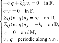 \begin{equation} \begin{cases} -\partial _i q +\partial ^2_{kk}v_i=0 \quad \text {in $\mathbb {F}$},\\[2pt] \partial _i v_i=0 \quad \text {in $\mathbb {F}$},\\ \Sigma _{ij}(v_\cdot ,q) n_j=a_i \quad \text {on $\mathbb {U}$},\\ \Sigma _{ij}(v_\cdot ,q) n_j={-}b_i \quad \text {on $\mathbb {D}$},\\[2pt] v_i=0 \quad \text {on $\partial \mathbb {M}$},\\ v_i,q \quad \text {periodic along $t_i$,$s_i$}, \end{cases} \end{equation}
where
 \begin{align} a_i=(1,0,0), \, b_i=0 \text { for } M_{\cdot n},Q_n, \qquad & a_i=0, \, b_i=(1,0,0) \text { for } N_{\cdot n},R_n, \end{align}
 \begin{align} a_i=(0,1,0), \, b_i=0 \text { for } M_{\cdot t},Q_t, \qquad & a_i=0, \, b_i=(0,1,0) \text { for } N_{\cdot t},Q_t, \end{align}
 \begin{align} a_i=(0,0,1), \, b_i=0 \text { for } M_{\cdot s},Q_s, \qquad & a_i=0, \, b_i=(0,0,1) \text { for } N_{\cdot s},R_s, \end{align}
and the unitary vector $r_i$
is used to select the
$r_i$
is used to select the $i$
th component of
$i$
th component of $M_{ij}$
or
$M_{ij}$
or $N_{ij}$
to be averaged,
$N_{ij}$
to be averaged,
 \begin{align} r_i=(1,0,0) \quad \text { to select } \bar {M}_{n\cdot } \text { or } \bar {N}_{n\cdot }, \end{align}
 \begin{align} r_i=(0,1,0) \quad \text { to select } \bar {M}_{t\cdot } \text { or } \bar {N}_{t\cdot }, \end{align}
 \begin{align} r_i=(0,0,1) \quad \text { to select } \bar {M}_{s\cdot } \text { or } \bar {N}_{s\cdot }, \end{align}
as shown in the schematic figure 12.
Schematic visualisation of the compact notation and averaging when $\boldsymbol {n}=(1,0,0),\boldsymbol {t}=(0,1,0), \boldsymbol {s}=(0,0,1)$
: the
$\boldsymbol {n}=(1,0,0),\boldsymbol {t}=(0,1,0), \boldsymbol {s}=(0,0,1)$
: the $M_{ij}$
and
$M_{ij}$
and $N_{ij}$
tensors are decomposed column by column into a sequence of six independent problems for
$N_{ij}$
tensors are decomposed column by column into a sequence of six independent problems for $(v_i,q)$
. The rowwise selection of the ‘observed’ component of
$(v_i,q)$
. The rowwise selection of the ‘observed’ component of $v_i$
(i.e. the component whose average is considered) in the computation of the first-order Lagrangian (2.21) is done via the unitary vector
$v_i$
(i.e. the component whose average is considered) in the computation of the first-order Lagrangian (2.21) is done via the unitary vector $\boldsymbol {r}$
.
$\boldsymbol {r}$
.
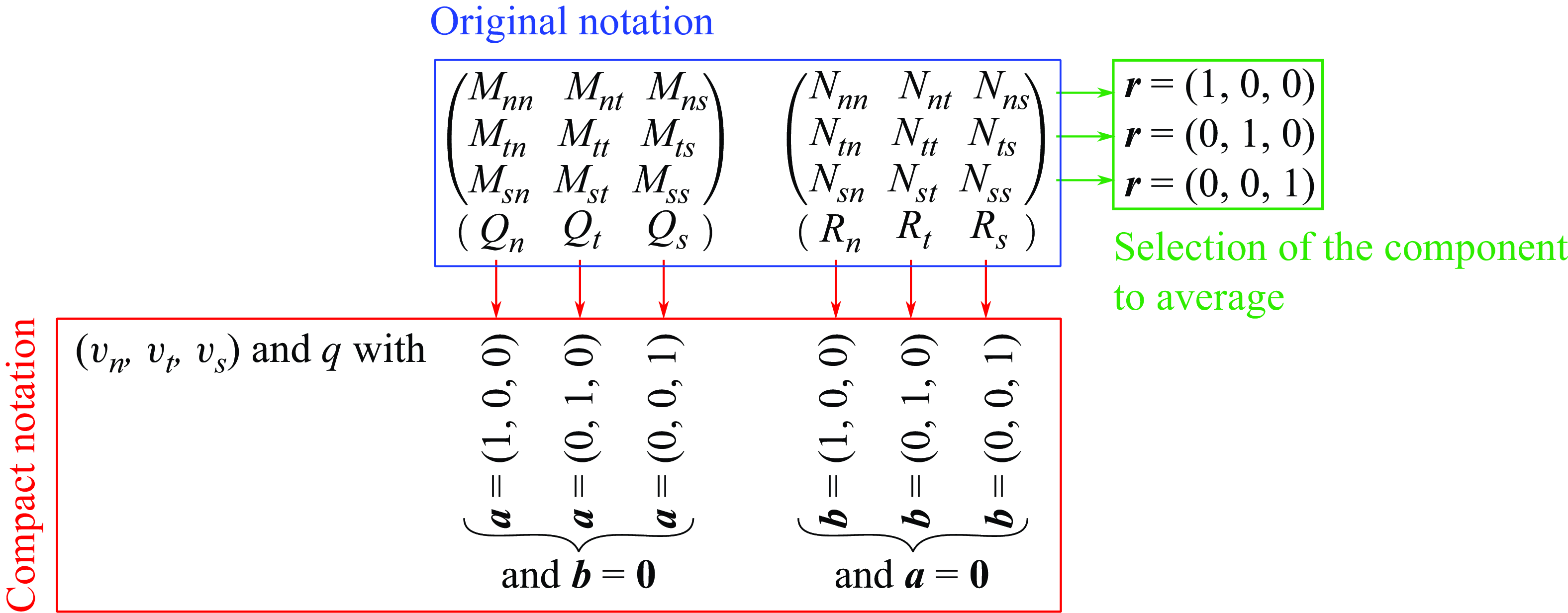
We clarify the meaning of the compact notation in a 2-D domain where $n_i=(1,0)$
and
$n_i=(1,0)$
and $t_i=(0,1)$
:
$t_i=(0,1)$
:
-
(i) to find
$(M_{nn},M_{tn})$
and
$Q_n$
we solve(A8)which, respectively, means
\begin{equation} \begin{cases} -\partial _i q +\partial ^2_{kk}v_i=0 \quad \text {in $\mathbb {F}$},\\ \partial _i v_i=0 \quad \text {in $\mathbb {F}$},\\ \Sigma _{ij}(v_\cdot ,q) n_j =(1,0) \quad \text {on $\mathbb {U}$},\\ \Sigma _{ij}(v_\cdot ,q) n_i = 0 \quad \text {on $\mathbb {D}$},\\ v_i=0 \quad \text {on $\partial \mathbb {M}$},\\ v_i,q \quad \text {periodic along $t_i$}, \end{cases} \!\!\quad \text { equivalent to}\! \quad \begin{cases} -\partial _i Q_{n} +\partial ^2_{kk}M_{in}=0 \quad \text {in $\mathbb {F}$},\\ \partial _i M_{in}=0 \quad \text {in $\mathbb {F}$},\\ \Sigma _{hj}(M_{\cdot n},Q_n) n_j =(1,0) \quad \text {on $\mathbb {U}$},\\ \Sigma _{hj}(M_{\cdot n},Q_n) n_j =0 \quad \text {on $\mathbb {D}$},\\ M_{in}=0 \quad \text {on $\partial \mathbb {M}$},\\ M_{in},Q_{n} \quad \text {periodic along $t_i$}, \end{cases} \end{equation}
(A9)
\begin{equation} \begin{cases} -\partial _i q +\partial ^2_{nn}v_n+\partial ^2_{tt}v_n=0 \quad \text {in $\mathbb {F}$},\\[3pt] -\partial _i q +\partial ^2_{nn}v_t+\partial ^2_{tt}v_t=0 \quad \text {in $\mathbb {F}$},\\[1pt] \partial _n v_n+\partial _t v_t=0 \quad \text {in $\mathbb {F}$},\\ -q+2\partial _n v_n =-1 \quad \text {on $\mathbb {U}$},\\ \partial _n v_t + \partial _t v_n =0 \quad \text {on $\mathbb {U}$},\\ -q+2\partial _n v_n =0 \quad \text {on $\mathbb {D}$},\\ \partial _n v_t + \partial _t v_n =0 \quad \text {on $\mathbb {D}$},\\ v_n,v_t=0 \quad \text {on $\partial \mathbb {M}$},\\ v_n,v_t,q \quad \text {periodic along $(1,0)$}, \end{cases} \quad \!\!\text {and}\! \quad \begin{cases} -\partial _i Q_{n} +\partial ^2_{nn}M_{nn} +\partial ^2_{tt}M_{nn}=0 \quad \text {in $\mathbb {F}$},\\[3pt] -\partial _i Q_{n} +\partial ^2_{nn}M_{tn} +\partial ^2_{tt}M_{tn}=0 \quad \text {in $\mathbb {F}$},\\[3pt] \partial _n M_{nn}+\partial _t M_{tn}=0 \quad \text {in $\mathbb {F}$},\\ -Q_n+2\partial _n M_{nn} =-1 \quad \text {on $\mathbb {U}$},\\ \partial _n M_{tn} + \partial _t M_{nn} =0 \quad \text {on $\mathbb {U}$},\\ -Q_n+2\partial _n M_{nn} =0 \quad \text {on $\mathbb {D}$},\\ \partial _n M_{tn} + \partial _t M_{nn} =0 \quad \text {on $\mathbb {D}$},\\ M_{nn},M_{tn}=0 \quad \text {on $\partial \mathbb {M}$},\\ M_{nn},M_{tn},Q_{n} \quad \text {periodic along $(1,0)$}; \end{cases} \end{equation}
-
(ii) to find
$(M_{nt},M_{tt})$
and
$Q_t$
we solve(A10)which, respectively, mean
\begin{equation} \begin{cases} -\partial _i q +\partial ^2_{kk}v_i=0 \quad \text {in $\mathbb {F}$},\\[2pt] \partial _i v_i=0 \quad \text {in $\mathbb {F}$},\\ \Sigma _{ij}(v_\cdot ,q) n_j =(0,1) \quad \text {on $\mathbb {U}$},\\ \Sigma _{ij}(v_\cdot ,q) n_i = 0 \quad \text {on $\mathbb {D}$},\\ v_i=0 \quad \text {on $\partial \mathbb {M}$},\\ v_i,q \quad \text {periodic along $t_i$}, \end{cases} \quad \text {equivalent to} \quad \begin{cases} -\partial _i Q_{t} +\partial ^2_{kk}M_{it}=0 \quad \text {in $\mathbb {F}$},\\[2pt] \partial _i M_{it}=0 \quad \text {in $\mathbb {F}$},\\ \Sigma _{hj}(M_{\cdot t},Q_t) n_j =(0,1) \quad \text {on $\mathbb {U}$},\\ \Sigma _{hj}(M_{\cdot t},Q_t) n_j =0 \quad \text {on $\mathbb {D}$},\\ M_{it}=0 \quad \text {on $\partial \mathbb {M}$},\\ M_{it},Q_{t} \quad \text {periodic along $t_i$}, \end{cases} \end{equation}
(A11)
\begin{equation} \begin{cases} -\partial _i q +\partial ^2_{nn}v_n+\partial ^2_{tt}v_n=0 \quad \text {in $\mathbb {F}$},\\[3pt] -\partial _i q +\partial ^2_{nn}v_t+\partial ^2_{tt}v_t=0 \quad \text {in $\mathbb {F}$},\\[3pt] \partial _n v_n+\partial _t v_t=0 \quad \text {in $\mathbb {F}$},\\ -q+2\partial _n v_n =0 \quad \text {on $\mathbb {U}$},\\ \partial _n v_t + \partial _t v_n =-1 \quad \text {on $\mathbb {U}$},\\ -q+2\partial _n v_n =0 \quad \text {on $\mathbb {D}$},\\ \partial _n v_t + \partial _t v_n =0 \quad \text {on $\mathbb {D}$},\\ v_n,v_t=0 \quad \text {on $\partial \mathbb {M}$},\\ v_n,v_t,q \quad \text {periodic along $(1,0)$}, \end{cases} \!\!\quad \text {and} \quad \begin{cases} -\partial _i Q_{t} +\partial ^2_{nn}M_{nt} +\partial ^2_{tt}M_{nt}=0 \quad \text {in $\mathbb {F}$},\\[3pt] -\partial _i Q_{t} +\partial ^2_{nn}M_{tt} +\partial ^2_{tt}M_{tt}=0 \quad \text {in $\mathbb {F}$},\\[3pt] \partial _n M_{nt}+\partial _t M_{tt}=0 \quad \text {in $\mathbb {F}$},\\ -Q_t+2\partial _n M_{nt} =0 \quad \text {on $\mathbb {U}$},\\ \partial _n M_{tt} + \partial _t M_{nt} =-1 \quad \text {on $\mathbb {U}$},\\ -Q_t+2\partial _n M_{nt} =0 \quad \text {on $\mathbb {D}$},\\ \partial _n M_{tt} + \partial _t M_{nt} =0 \quad \text {on $\mathbb {D}$},\\ M_{nt},M_{tt}=0 \quad \text {on $\partial \mathbb {M}$},\\ M_{nt},M_{tt},Q_{t} \quad \text {periodic along $(1,0)$}; \end{cases} \end{equation}
-
(iii) to find
$(N_{nn},N_{tn})$
and
$R_n$
we solve(A12)
\begin{equation} \begin{cases} -\partial _i q +\partial ^2_{kk}v_i=0 \quad \text {in $\mathbb {F}$},\\[3pt] \partial _i v_i=0 \quad \text {in $\mathbb {F}$},\\ \Sigma _{ij}(v_\cdot ,q) n_j = 0 \quad \text {on $\mathbb {U}$},\\ \Sigma _{ij}(v_\cdot ,q) n_i = ({-}1,0) \quad \text {on $\mathbb {D}$},\\ v_i=0 \quad \text {on $\partial \mathbb {M}$},\\ v_i,q \quad \text {periodic along $t_i$}, \end{cases} \!\!\!\!\quad \text {equivalent to} \!\!\!\!\quad \begin{cases} -\partial _i R_{n} +\partial ^2_{kk}N_{in}=0 \quad \text {in $\mathbb {F}$},\\[3pt] \partial _i N_{in}=0 \quad \text {in $\mathbb {F}$},\\ \Sigma _{hj}(N_{\cdot n},R_n) n_j =0 \quad \text {on $\mathbb {U}$},\\ \Sigma _{hj}(N_{\cdot n},R_n) n_j =({-}1,0) \quad \text {on $\mathbb {D}$},\\ N_{in}=0 \quad \text {on $\partial \mathbb {M}$},\\ N_{in},R_{n} \quad \text {periodic along $t_i$}; \end{cases} \end{equation}
-
(iv) to find
$(N_{nt},N_{tt})$
and
$R_t$
we solve(A13)
\begin{equation} \begin{cases} -\partial _i q +\partial ^2_{kk}v_i=0 \quad \text {in}\ \mathbb {F},\\[3pt] \partial _i v_i=0 \quad \text {in}\ \mathbb {F},\\ \Sigma _{ij}(v_\cdot ,q) n_j =0 \quad \text {on}\ \mathbb {U},\\ \Sigma _{ij}(v_\cdot ,q) n_i =(0,{-}1) \!\quad \text {on}\ \mathbb {D},\\ v_i=0 \quad \text{on}\ \partial \mathbb {M},\\ v_i,q \quad \text {periodic along}\ t_i, \end{cases} \!\!\!\!\!\quad \text {equivalent to} \!\!\!\quad \begin{cases} -\partial _i R_{t} +\partial ^2_{kk}N_{it}=0 \quad \text {in}\ \mathbb {F},\\[3pt] \partial _i N_{it}=0 \quad \text {in}\ \mathbb {F},\\ \Sigma _{hj}(N_{\cdot t},R_t) n_j =0 \quad \text {on}\ \mathbb {U},\\ \Sigma _{hj}(N_{\cdot t},R_t) n_j =(0,{-}1) \quad \text {on}\ \mathbb {D},\\ N_{it}=0 \quad \text {on}\ \partial \mathbb {M},\\ N_{it},R_{t} \quad \text {periodic along}\ t_i. \end{cases} \end{equation}


We now provide an explicit example of how we can calculate the shape sensitivities for the Navier tensor component $\bar {M}_{nn}$
. We produced figure 5(a,d,g) by solving the equations provided in the present appendix in a 2-D domain with a circular solid inclusion of radius
$\bar {M}_{nn}$
. We produced figure 5(a,d,g) by solving the equations provided in the present appendix in a 2-D domain with a circular solid inclusion of radius $R_A$
. The remaining tensor components follow the nomenclature provided in schematic figure 12.
$R_A$
. The remaining tensor components follow the nomenclature provided in schematic figure 12.
To find how a change in shape $\beta$
affects
$\beta$
affects $\bar {M}_{nn}$
, we need to evaluate (2.36) with
$\bar {M}_{nn}$
, we need to evaluate (2.36) with $v_i=M_{in}$
and
$v_i=M_{in}$
and $\boldsymbol {r}=(1,0)$
, i.e.
$\boldsymbol {r}=(1,0)$
, i.e.
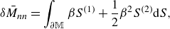 \begin{equation} \delta \bar {M}_{nn}=\int _{\partial \mathbb {M}}\beta S^{(1)}+\frac {1}{2}\beta ^2 S^{(2)} {\rm d}S, \end{equation}
where, on a 2-D circular inclusion such as the one in figure 3(a), ${\rm d}S=R_A{\rm d}\theta$
and the sensitivities
${\rm d}S=R_A{\rm d}\theta$
and the sensitivities $S^{(1)}$
and
$S^{(1)}$
and $S^{(2)}$
are specialised for
$S^{(2)}$
are specialised for $M_{in}$
, i.e.
$M_{in}$
, i.e.
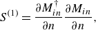 \begin{align} S^{(1)}=\frac {\partial M_{in}^{\dagger }}{\partial n}\frac {\partial M_{in}}{\partial n},\qquad\qquad\qquad\qquad\qquad \end{align}
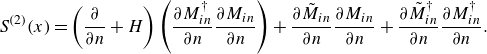 \begin{align} S^{(2)}(x) = \left ( \frac {\partial }{\partial n}+H \right ) \left ( \frac {\partial M_{in}^\dagger }{\partial n}\frac {\partial M_{in}}{\partial n} \right ) + \frac {\partial \tilde {M}_{in}}{\partial n}\frac {\partial M_{in}}{\partial n} + \frac {\partial \tilde {M}_{in}^\dagger }{\partial n}\frac {\partial M_{in}^\dagger }{\partial n}. \end{align}
These fields are found by solving the direct and adjoint problems, i.e.
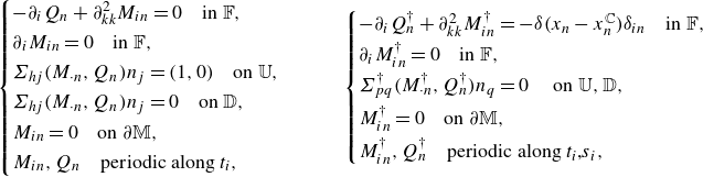 \begin{align} \begin{cases} -\partial _i Q_{n} +\partial ^2_{kk}M_{in}=0 \quad \text {in $\mathbb {F}$},\\[2pt] \partial _i M_{in}=0 \quad \text {in $\mathbb {F}$},\\[2pt] \Sigma _{hj}(M_{\cdot n},Q_n) n_j =(1,0) \quad \text {on $\mathbb {U}$},\\[2pt] \Sigma _{hj}(M_{\cdot n},Q_n) n_j =0 \quad \text {on $\mathbb {D}$},\\[2pt] M_{in}=0 \quad \text {on $\partial \mathbb {M}$},\\[2pt] M_{in},Q_{n} \quad \text {periodic along $t_i$}, \end{cases} \qquad \begin{cases} -\partial _i Q_{n}^{\dagger } +\partial ^2_{kk}M_{in}^{\dagger }=-\delta (x_n-x_n^{\mathbb {C}})\delta _{in} \quad \text {in $\mathbb {F}$},\\[2pt] \partial _i M_{in}^{\dagger }=0 \quad \text {in $\mathbb {F}$},\\[2pt] \Sigma _{pq}^\dagger (M_{\cdot n}^{\dagger },Q_{n}^{\dagger })n_q=0 \quad \text { on $\mathbb {U,D}$},\\[3pt] M_{in}^{\dagger }=0 \quad \text {on $\partial \mathbb {M}$},\\[3pt] M_{in}^{\dagger },Q_n^{\dagger } \quad \text {periodic along $t_i$,$s_i$}, \end{cases} \end{align}
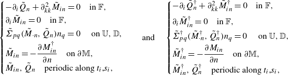 \begin{align} \begin{cases} -\partial _i \tilde {Q}_n +\partial ^2_{kk}\tilde {M}_{in}=0 \quad \text {in $\mathbb {F}$}, \\[2pt] \partial _i \tilde {M}_{in}=0 \quad \text {in $\mathbb {F}$}, \\[2pt] \tilde {\Sigma }_{pq}(\tilde {M}_{\cdot n},\tilde {Q}_n)n_q=0 \quad \text { on $\mathbb {U,D}$}, \\[2pt] \tilde {M}_{in} = -\dfrac {\partial M_{in}^{\dagger }}{\partial n} \quad \text {on $\partial \mathbb {M}$}, \\[3pt] \tilde {M}_{in},\tilde {Q}_n \quad \text {periodic along $t_i$,$s_i$}, \end{cases} \quad \text {and} \quad \begin{cases} -\partial _i \tilde {Q}_n^{\dagger } +\partial ^2_{kk}\tilde {M}_{in}^{\dagger }=0 \quad \text {in $\mathbb {F}$}, \\[5pt] \partial _i \tilde {M}_{in}^{\dagger }=0 \quad \text {in $\mathbb {F}$}, \\[3pt] \tilde {\Sigma }^{\dagger }_{pq}(\tilde {M}_{\cdot n}^{\dagger },\tilde {Q}_n^{\dagger })n_q=0 \quad \text { on $\mathbb {U,D}$}, \\[3pt] \tilde {M}^{\dagger }_{in} = -\dfrac {\partial M_{in}}{\partial n} \quad \text {on $\partial \mathbb {M}$}, \\[5pt] \tilde {M}^{\dagger }_{in},\tilde {Q}_n^{\dagger } \quad \text {periodic along $t_i$,$s_i$}, \end{cases} \quad\end{align}
on a reference configuration, e.g. $R_A=0.12, R_B=0.15, x_t^A=0.2$
and
$R_A=0.12, R_B=0.15, x_t^A=0.2$
and $ x_t^B=-0.2$
, as in figure 4(a–d), corresponding to the green curves of figure 5(a,d). Now we can reconstruct the green dotted lines in figure 5(g) by simply evaluating (B14) with
$ x_t^B=-0.2$
, as in figure 4(a–d), corresponding to the green curves of figure 5(a,d). Now we can reconstruct the green dotted lines in figure 5(g) by simply evaluating (B14) with $\beta =\Delta R_A$
(the variation in radius
$\beta =\Delta R_A$
(the variation in radius $R_A$
from the reference configuration) and summing
$R_A$
from the reference configuration) and summing $\delta \bar {M}_{nn}$
to the
$\delta \bar {M}_{nn}$
to the $\bar {M}_{nn}$
of the reference configuration (i.e. the average solution of the first problem in (B17)).
$\bar {M}_{nn}$
of the reference configuration (i.e. the average solution of the first problem in (B17)).
Appendix B. Numerical implementation and mesh independence study
In the present study, we carried out simulations using the finite-element software COMSOL Multiphysics. We employed P3-P2 elements (for velocity and pressure, respectively) in all the microscopic simulations, and P2-P1 elements in the macroscopic and full-scale simulations. Elements are quadrilaterals in the boundary layers and triangles everywhere else. The mesh independence in the microscopic simulations was tested for the microscopic domain size, the amplitude of the numerical Dirac delta function and the mesh thickness. The study regarding the microscopic domain size shows the same trends as Zampogna & Gallaire (Reference Zampogna and Gallaire2020), thus it will not be repeated here. The Dirac delta function has been modelled using a Gaussian function
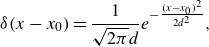 \begin{equation} \delta (x-x_0)=\frac {1}{\sqrt {2\pi }d}e^{-\frac {(x-x_0)^2}{2d^2}}, \end{equation}
discretised with $10$
mesh elements in the normal direction. In the present simulations, we found that
$10$
mesh elements in the normal direction. In the present simulations, we found that $d=0.005$
is a good compromise between cost and accuracy, as shown in figure 13(
$d=0.005$
is a good compromise between cost and accuracy, as shown in figure 13( $d$
). The convergence with respect to the mesh refinement has been studied considering a mesh having typical sizes of
$d$
). The convergence with respect to the mesh refinement has been studied considering a mesh having typical sizes of $0.001l$
on the solid inclusion, as well as eight quadrilateral layers, and
$0.001l$
on the solid inclusion, as well as eight quadrilateral layers, and $0.03l$
far from it. This mesh has been modified by dividing these sizes by a factor of
$0.03l$
far from it. This mesh has been modified by dividing these sizes by a factor of $k$
. Figure 13(
$k$
. Figure 13( $c$
) shows that for
$c$
) shows that for $k=1$
the mesh-related error concerning the integral value of the second-order sensitivity on the solid inclusion is smaller than
$k=1$
the mesh-related error concerning the integral value of the second-order sensitivity on the solid inclusion is smaller than $1\,\%$
between two subsequent meshes. The influence of the mesh in the full-scale and macroscopic simulations has been studied similarly, as shown in figure 13(
$1\,\%$
between two subsequent meshes. The influence of the mesh in the full-scale and macroscopic simulations has been studied similarly, as shown in figure 13( $a,\!b$
). In this case, the mesh sizes corresponding to
$a,\!b$
). In this case, the mesh sizes corresponding to $k=1$
are
$k=1$
are
-
(i) for the full-scale simulation:
$5\times 10^{-4}$
on the solid inclusions and
$0.05$
far from them, with an enclosure around the membrane having a typical mesh size of
$0.01$
; -
(ii) for the macroscopic simulation:
$0.0025$
on the interface and
$0.05$
far from it.


Mesh independence study. Total force $F_{tot}=|\int _{\partial \mathbb {M}}\Sigma _{ij}n_j|$
exerted by the fluid on the membrane in the full-scale simulation (
$F_{tot}=|\int _{\partial \mathbb {M}}\Sigma _{ij}n_j|$
exerted by the fluid on the membrane in the full-scale simulation ( $a$
) and in the macroscopic simulation (
$a$
) and in the macroscopic simulation ( $b$
) as a function of the mesh factor
$b$
) as a function of the mesh factor $k$
. The integral of the second-order shape sensitivity of
$k$
. The integral of the second-order shape sensitivity of $\bar {M}_{nn}$
as a function of the mesh factor
$\bar {M}_{nn}$
as a function of the mesh factor $k$
(
$k$
( $c$
) and the numerical Dirac delta function amplitude
$c$
) and the numerical Dirac delta function amplitude $d$
(
$d$
( $d$
) in the microscopic simulation.
$d$
) in the microscopic simulation.
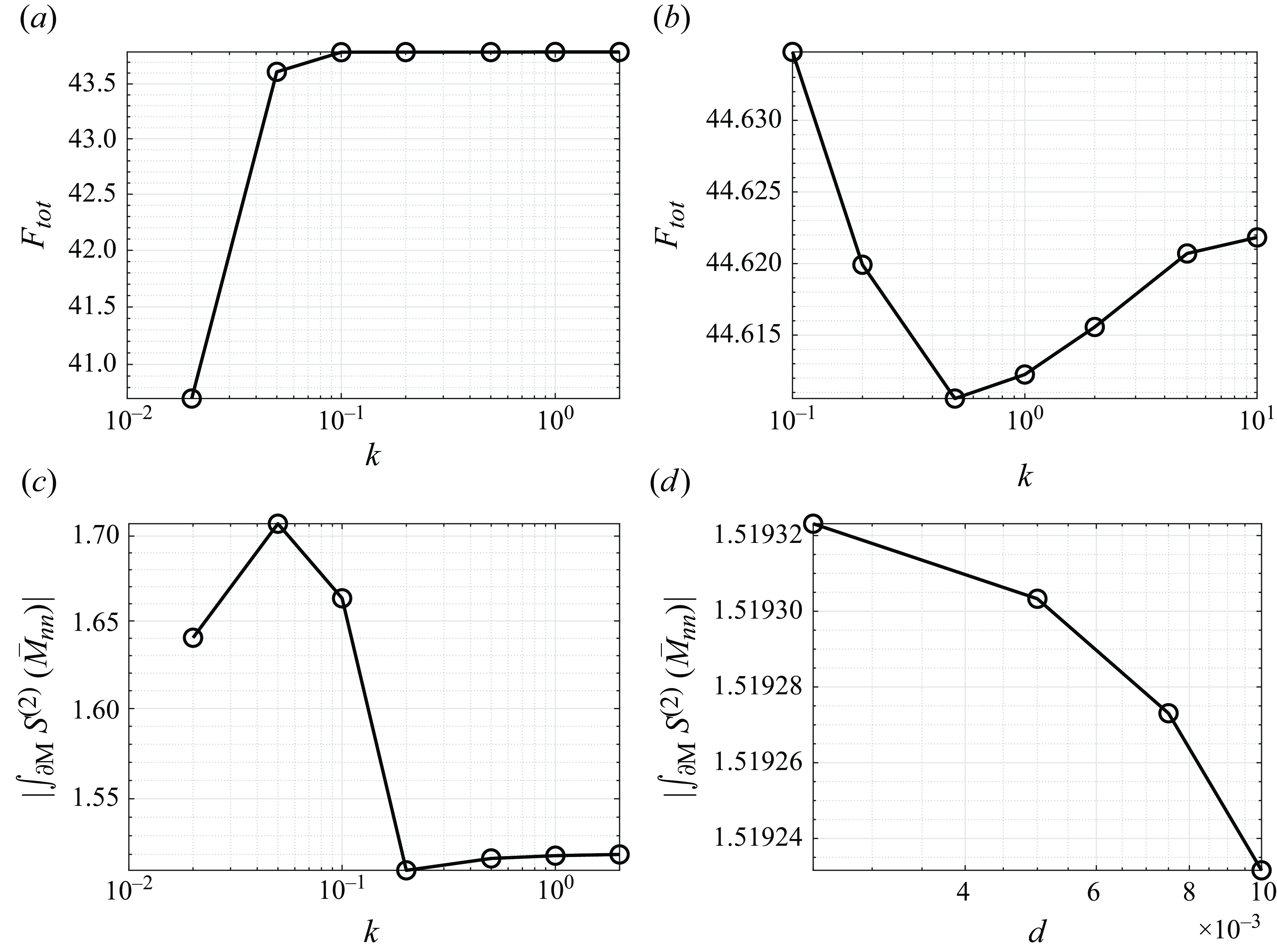
In both cases, for $k=1$
, the module of the force exerted on the membrane
$k=1$
, the module of the force exerted on the membrane $F_{tot}$
changes between two subsequent meshes less than
$F_{tot}$
changes between two subsequent meshes less than $1\,\%$
.
$1\,\%$
.
Appendix C. About the oscillations of the second-order sensitivity
In this section, we discuss the influence of the oscillations around the locations $\theta =\pi /2$
and
$\theta =\pi /2$
and $3\pi /2$
of the second order sensitivity
$3\pi /2$
of the second order sensitivity $S^{(2)}(\bar {M}_{tt})$
in figures 7(
$S^{(2)}(\bar {M}_{tt})$
in figures 7( $a$
) and 6(
$a$
) and 6( $a,\!c$
). To show their numerical nature, we consider the geometry corresponding to the black stars in figure 7(
$a,\!c$
). To show their numerical nature, we consider the geometry corresponding to the black stars in figure 7( $c,\!d$
) (i.e.
$c,\!d$
) (i.e. $l_n=l_t=r=0.15$
) and a base mesh whose sizing is
$l_n=l_t=r=0.15$
) and a base mesh whose sizing is
-
(i)
$0.001$
inside a zone large
$d=0.01$
around
$x_n=0$
and on the solid inclusion; -
(ii)
$0.02$
far from the solid inclusion;


Integral of the second order sensitivity $S^{(2)}$
for the component
$S^{(2)}$
for the component $\bar {M}_{tt}$
along the solid inclusion (left-hand axis, blue) and its standard deviation with respect to a low-pass filtered signal
$\bar {M}_{tt}$
along the solid inclusion (left-hand axis, blue) and its standard deviation with respect to a low-pass filtered signal $\tilde {S}^{(2)}$
(right-hand axis, red) in the window
$\tilde {S}^{(2)}$
(right-hand axis, red) in the window $\theta \in [\pi /2-d/(2r),\pi /2+d/(2r)]$
, for a range of the mesh size parameter
$\theta \in [\pi /2-d/(2r),\pi /2+d/(2r)]$
, for a range of the mesh size parameter $a$
. The low-pass filter has a step response at a wavelength of
$a$
. The low-pass filter has a step response at a wavelength of $d/2$
, to eliminate the oscillations caused by the Dirac delta function.
$d/2$
, to eliminate the oscillations caused by the Dirac delta function.
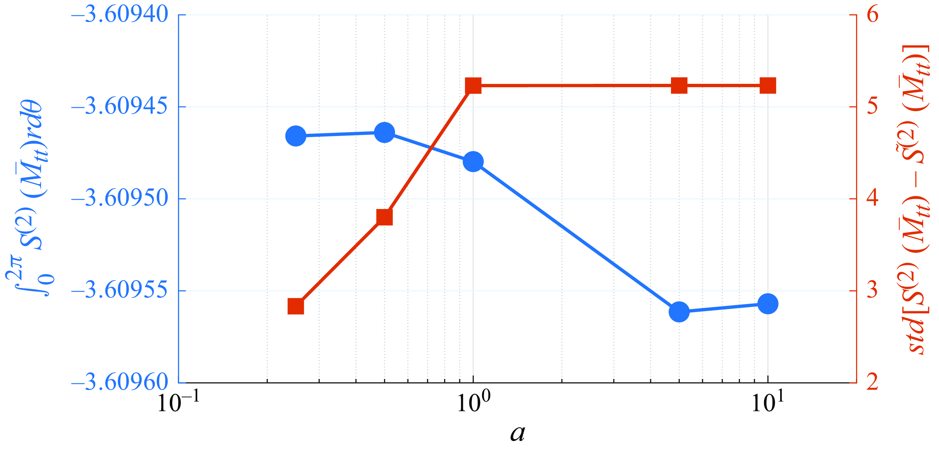
and change only the discretisation in the zone of amplitude $d$
including the numerical Dirac delta function by multiplying the mesh sizes by a factor
$d$
including the numerical Dirac delta function by multiplying the mesh sizes by a factor $a$
. In figure 14, we compare the integral of the second-order sensitivity and its standard deviation with respect to a low-pass filtered signal
$a$
. In figure 14, we compare the integral of the second-order sensitivity and its standard deviation with respect to a low-pass filtered signal $\tilde {S}^{(2)}$
for
$\tilde {S}^{(2)}$
for $a\in [0.25,10]$
. The oscillations of the second order sensitivity decrease in amplitude as the mesh is refined (lower
$a\in [0.25,10]$
. The oscillations of the second order sensitivity decrease in amplitude as the mesh is refined (lower $a$
) and its integral value along
$a$
) and its integral value along $\partial \mathbb {M}$
has relative variations below
$\partial \mathbb {M}$
has relative variations below $0.01\,\%$
. We conclude that these oscillations can be suppressed with high mesh refinement, however, they do not influence the conclusions drawn in § 3.
$0.01\,\%$
. We conclude that these oscillations can be suppressed with high mesh refinement, however, they do not influence the conclusions drawn in § 3.


 Open access