





1. Introduction
Anisotropy of the Reynolds stress tensor is one of the fundamental characteristics of most turbulent flows in natural, engineering and technological applications (e.g. Burchard & Bolding Reference Burchard and Bolding2001; Biferale & Procaccia Reference Biferale and Procaccia2005; Klipp Reference Klipp2014; Mishra, Iaccarino & Duraisamy Reference Mishra, Iaccarino and Duraisamy2016; Klipp Reference Klipp2018). At large scales, turbulence rarely attains a kinetic energy state that is equipartitioned between the three velocity components or a state where turbulent stresses disappear. Such an isotropic state would ‘rob’ turbulence of its most important characteristic – efficient momentum transport. In fact, turbulence is almost always anisotropic as a result of the generation of turbulence kinetic energy (TKE) along specific directions. In atmospheric flows, two processes dominate anisotropy production: shear injects energy preferentially in the streamwise direction, while buoyancy acts in the vertical direction, either as a source (unstable stratification) or sink (stable stratification) of TKE. Close to a solid surface, turbulence additionally experiences wall blocking (Pope Reference Pope2000), limiting the energy in the wall-normal direction (e.g. Hunt & Graham Reference Hunt and Graham1978; Durbin Reference Durbin1991; Perot & Moin Reference Perot and Moin1995), with further influences on anisotropy occurring through the action of roughness (Smalley et al. Reference Smalley, Leonardi, Antonia, Djenidi and Orlandi2002), curvature (So Reference So1977; Moser & Moin Reference Moser and Moin1987), rotation (Kassinos & Reynolds Reference Kassinos and Reynolds1997) and non-local effects (Mishra et al. Reference Mishra, Iaccarino and Duraisamy2016). On the other hand, all turbulent flows experience a pressure-strain interaction that acts to redistribute TKE towards the less-energetic velocity components and decorrelate componentwise velocity fluctuations, driving turbulence towards an equipartitioned and stress-free state. This process of ‘pressure redistribution’ remains an area of active research (e.g. Jaw & Chen Reference Jaw and Chen1998; Kassinos, Reynolds & Rogers Reference Kassinos, Reynolds and Rogers2001; Alfonsi Reference Alfonsi2009; Nguyen et al. Reference Nguyen, Horst, Oncley and Tong2013; Chaouat Reference Chaouat2017; Ding et al. Reference Ding, Nguyen, Liu, Otte and Tong2018; Ayet et al. Reference Ayet, Katul, Bragg and Redelsperger2020; Homan, Shende & Mani Reference Homan, Shende and Mani2024; Liu, Ahmed & Chakraborty Reference Liu, Ahmed and Chakraborty2024; Yi, Koseff & Bou-Zeid Reference Yi, Koseff and Bou-Zeid2025). The anisotropic state of turbulence for a particular flow, therefore, is a result of the interplay between the efficiency of the anisotropy generation mechanisms versus its reduction by the pressure-strain interactions.
Atmospheric boundary layer turbulence is a particularly consequential manifestation of wall-bounded turbulence, characterised by a very high Reynolds number and prevalent stratification that has an appreciable impact on turbulence, especially through the evolution of turbulence into large-scale organised structures (Hutchins et al. Reference Hutchins, Chauhan, Marusic, Monty and Klewicki2012). In fact, atmospheric turbulence is hardly ever truly neutrally stratified (Li et al. Reference Li, Hutchins, Zheng, Marusic and Baars2022), and stratification has been shown to influence not only the production of Reynolds stress anisotropy (not to be interpreted as anisotropy of the length scales related to coherent structures), but also the pressure redistribution (Nguyen et al. Reference Nguyen, Horst, Oncley and Tong2013; Bou-Zeid et al. Reference Bou-Zeid, Gao, Ansorge and Katul2018), leading to lingering flow anisotropy even at inertial-subrange scales (Praskovsky et al. Reference Praskovsky, Gledzer, Karyakin and Zhou1993; Katul, Hsieh & Sigmon Reference Katul, Hsieh and Sigmon1997; Stiperski et al. Reference Stiperski, Katul and Calaf2021b ; Chowdhuri & Banerjee Reference Chowdhuri and Banerjee2024).
Early work by Kader & Yaglom (Reference Kader and Yaglom1990) suggested that such anisotropic nature of turbulence is of particular interest in the atmospheric surface layer (ASL), where it has recently been shown to act as an additional non-dimensional group in surface-layer scaling (Stiperski & Calaf Reference Stiperski and Calaf2023; Mosso, Calaf & Stiperski Reference Mosso, Calaf and Stiperski2024; Charrondière & Stiperski Reference Charrondière and Stiperski2024; Waterman et al. Reference Waterman, Stiperski, Chaney and Calaf2026), as well as in the universal nature of the scalewise relaxation to isotropy (Stiperski et al. Reference Stiperski, Katul and Calaf2021b ). The ability of the degree of anisotropy, quantified by the third invariant of the anisotropy stress tensor (Choi & Lumley Reference Choi and Lumley2001; Banerjee et al. Reference Banerjee, Krahl, Durst and Zenger2007), to collapse the scaled variances, gradients and spectra over a wide range of vastly different terrain complexities – where basic assumptions of boundary layer theories (planar homogeneity, flat terrain, no subsidence) are clearly violated and common scaling approaches fail (e.g. Sfyri et al. Reference Sfyri, Rotach, Stiperski, Bosveld, Manuela and Obleitner2018; Stiperski & Calaf Reference Stiperski and Calaf2018; Stiperski, Calaf & Rotach Reference Stiperski, Calaf and Rotach2019; Finnigan et al. Reference Finnigan, Ayotte, Harman, Katul, Oldroyd, Patton, Poggi, Ross and Taylor2020) – means that anisotropy encodes much of the complexity of the flow and surface conditions driving the turbulent flow (Chowdhuri & Banerjee Reference Chowdhuri and Banerjee2024; Mosso, Lapo & Stiperski Reference Mosso, Lapo and Stiperski2025; Waterman et al. Reference Waterman, Stiperski, Chaney and Calaf2026). Thus, understanding how specific states of anisotropy in turbulent energy (one-component, two-component, three-component) evolve under common conditions is of particular interest, but as of yet, this evolution is mostly based on plausibility arguments, symmetries and simplified budgets (cf. Stiperski & Calaf Reference Stiperski and Calaf2018; Ayet et al. Reference Ayet, Katul, Bragg and Redelsperger2020; Mosso et al. Reference Mosso, Lapo and Stiperski2025).
A way forward in understanding the evolution of Reynolds stress anisotropy is therefore to combine the budget equations that describe the evolution of the components of the Reynolds stress tensor with multi-level measurements collected over flat and planar homogeneous terrain, with the goal of unravelling the anisotropy drivers using revisions to conventional turbulence modelling perspectives.
To test how the common Reynolds stress budget models used in higher-order closures capture observed flow anisotropy, we leverage turbulence measurements from a range of observational campaigns. As a first approximation, we test how a reduced set of budget equations captures the observed energy anisotropy, i.e. how energy is distributed between the different velocity variances. This reduced model assumes a balance between shear and buoyancy production and dissipation, and models the return to isotropy using a linear Rotta scheme. This model provides expressions for normalised velocity variances as functions of the Richardson number, highlighting the change of anisotropy as stratification becomes progressively more dominant. These expressions then serve as a reference to an expanded version of the model that includes transport terms, as well as the pressure-strain parametrisation by adding the so-called rapid isotropisation of the production terms. Finally, the origins of the transport and rapid terms are explored.
The paper is organised as follows. In § 2 the Reynolds stress budgets, simplifications and closure assumptions are presented, in § 3 the datasets and turbulence data processing used are explained. Section 4 presents the results, further discussed in § 5, with conclusions presented in § 6.
2. Modelling the Reynolds stresses
2.1. Background and definitions
The conservation equations for the Reynolds stresses $\overline {u_i^{\prime} u_{\!j}^{\prime}}$
for an incompressible flow subject to the Boussinesq approximation, a linearised equation of state for air (ideal gas law), and hydrostatic equilibrium for the Boussinesq background state are given by (Launder, Reece & Rodi Reference Launder, Reece and Rodi1975; Stull Reference Stull1988; Pope Reference Pope2000)
$\overline {u_i^{\prime} u_{\!j}^{\prime}}$
for an incompressible flow subject to the Boussinesq approximation, a linearised equation of state for air (ideal gas law), and hydrostatic equilibrium for the Boussinesq background state are given by (Launder, Reece & Rodi Reference Launder, Reece and Rodi1975; Stull Reference Stull1988; Pope Reference Pope2000)
 \begin{align} \frac {\partial \overline {u_i^{\prime}u_{\!j}^{\prime}}}{\partial t}+\overline {U}_k\frac {\partial \overline {u_i^{\prime}u_{\!j}^{\prime}}}{\partial x_k} &= \underbrace {-\overline {u_{i}^{\prime}u_{k}^{\prime}}\frac {\partial \overline {U}_{\!j}}{\partial x_k}-\overline {u_{\!j}^{\prime}u_{k}^{\prime}}\frac {\partial \overline {U}_i}{\partial x_k}}_{2S_m} \underbrace {+\frac {g}{\overline {\theta }_{v0}}\left [\overline {u_i^{\prime}\theta _v^{\prime}}\delta _{j3} + \overline {u_{\!j}^{\prime}\theta _v^{\prime}}\delta _{i3}\right ]}_{2B} \nonumber \\ &\quad \underbrace {+f_c\left [\overline {u_i^{\prime}u_k^{\prime}}\epsilon _{jk3} + \overline {u_{\!j}^{\prime}u_k^{\prime}}\epsilon _{ik3}\right ]}_{Co} \underbrace {-\frac {\partial \overline {u_i^{\prime}u_{\!j}^{\prime}u_k^{\prime}}}{\partial x_k}}_{2T_{\textit{ij}}} \\ \nonumber &\quad \underbrace {\underbrace {-\frac {1}{\rho _0}\left [\frac {\partial \overline {u_i^{\prime}p'}}{\partial x_{\!j}} + \frac {\partial \overline {u_{\!j}^{\prime}p'}}{\partial x_i}\right ]}_{\varPi _{\textit{ij}}^{\textit{tr}}} + \underbrace {\frac {1}{\rho _0} \left [\overline {p' \left ( \frac {\partial u_i^{\prime}}{\partial x_{\!j}} + \frac {\partial u_{\!j}^{\prime}}{\partial x_i} \right ) }\right ]}_{\varPi _{\textit{ij}}^{\textit{str}}}}_{\varPi _{\textit{ij}}} -2\varepsilon _{u_i u_{{\kern-1pt}j}}, \end{align}
where $t$
is time,
$t$
is time, $\rho _o$
is the Boussinesq reference air density,
$\rho _o$
is the Boussinesq reference air density, $U_i=\overline {U_i}+u_i^{\prime}$
are the instantaneous velocity components along the
$U_i=\overline {U_i}+u_i^{\prime}$
are the instantaneous velocity components along the $x_i$
direction, where
$x_i$
direction, where $x_1$
,
$x_1$
, $x_2$
and
$x_2$
and $x_3$
are the streamwise (along mean wind direction), spanwise and wall-normal directions, respectively, and their corresponding velocity components are
$x_3$
are the streamwise (along mean wind direction), spanwise and wall-normal directions, respectively, and their corresponding velocity components are $u$
,
$u$
, $v$
and
$v$
and $w$
. The overline indicates Reynolds-averaged flow variables, primed quantities are fluctuations from their respective Reynolds-averaged state,
$w$
. The overline indicates Reynolds-averaged flow variables, primed quantities are fluctuations from their respective Reynolds-averaged state, $p'$
are the corresponding pressure fluctuations (the hydrostatic background pressure is already removed along with the gravity term),
$p'$
are the corresponding pressure fluctuations (the hydrostatic background pressure is already removed along with the gravity term), $\theta _v^{\prime}$
are the virtual potential temperature fluctuations (with their reference state
$\theta _v^{\prime}$
are the virtual potential temperature fluctuations (with their reference state $\overline {\theta }_{v0}$
corresponding to
$\overline {\theta }_{v0}$
corresponding to $\rho _0$
) and
$\rho _0$
) and $\varepsilon _{u_i u_{{\kern-1pt}j}}$
is the mean turbulent stress destruction rate due to the action of fluid viscosity
$\varepsilon _{u_i u_{{\kern-1pt}j}}$
is the mean turbulent stress destruction rate due to the action of fluid viscosity $\nu$
. The third term is a Coriolis redistribution term, which is not identically zero for the individual variances, but sums to zero for the TKE. In the budget equations, closure models for
$\nu$
. The third term is a Coriolis redistribution term, which is not identically zero for the individual variances, but sums to zero for the TKE. In the budget equations, closure models for $\varepsilon _{u_i u_{{\kern-1pt}j}}$
, the turbulent transport (
$\varepsilon _{u_i u_{{\kern-1pt}j}}$
, the turbulent transport ( $T_{\textit{ij}}$
) terms and the pressure-covariance term
$T_{\textit{ij}}$
) terms and the pressure-covariance term $\varPi _{\textit{ij}}$
(which can be decomposed into the pressure transport
$\varPi _{\textit{ij}}$
(which can be decomposed into the pressure transport $\varPi _{\textit{ij}}^{\textit{tr}}$
and pressure strain
$\varPi _{\textit{ij}}^{\textit{tr}}$
and pressure strain $\varPi _{\textit{ij}}^{\textit{str}}$
) are necessary.
$\varPi _{\textit{ij}}^{\textit{str}}$
) are necessary.
The most difficult and least understood among all these unclosed terms is $\varPi _{\textit{ij}}$
, which is commensurate in magnitude with the turbulence generation terms (the shear production, first term on the right-hand side of the equation, and buoyancy production/destruction, the second term). The reason for the difficulty in modelling
$\varPi _{\textit{ij}}$
, which is commensurate in magnitude with the turbulence generation terms (the shear production, first term on the right-hand side of the equation, and buoyancy production/destruction, the second term). The reason for the difficulty in modelling $\varPi _{\textit{ij}}$
is the fact that pressure perturbations
$\varPi _{\textit{ij}}$
is the fact that pressure perturbations $p'$
satisfy the Poisson equation given by (Hanjalić & Launder Reference Hanjalić and Launder1972; Launder et al. Reference Launder, Reece and Rodi1975)
$p'$
satisfy the Poisson equation given by (Hanjalić & Launder Reference Hanjalić and Launder1972; Launder et al. Reference Launder, Reece and Rodi1975)
 \begin{equation} \frac {1}{\rho _o} \boldsymbol{\nabla} ^2 p'= \underbrace {-2 \frac {\partial \overline {U_i}}{\partial x_{\!j}} \frac {\partial u_{\!j}^{\prime}}{\partial x_i}}_{\textit{Rapid}\,\textit{term}} \underbrace {-\frac {\partial ^2}{\partial x_i \partial x_{\!j}} \left (u_i^{\prime} u_{\!j}^{\prime} - \overline {u_i^{\prime} u_{\!j}^{\prime}}\right )}_{\textit{Slow}\,\textit{term}}+\underbrace {\frac {g}{\overline {\theta }_{v0}}\frac {\partial \theta_v^{\prime}}{\partial z}.}_{\textit{Buoyancy}\,\textit{term}} \end{equation}
This equation is elliptic – meaning that $p'$
at position
$p'$
at position $x_i$
requires knowledge of the flow field and temperature across the entire flow domain. Hence, local closure models that represent
$x_i$
requires knowledge of the flow field and temperature across the entire flow domain. Hence, local closure models that represent $\varPi _{\textit{ij}}$
as a function of only local velocity statistics (or their gradients) at
$\varPi _{\textit{ij}}$
as a function of only local velocity statistics (or their gradients) at $x_i$
cannot accommodate the non-local effects of velocity and temperature at distant points. Nonetheless, (2.2) underscores three mechanisms that historically formed the basis for modelling
$x_i$
cannot accommodate the non-local effects of velocity and temperature at distant points. Nonetheless, (2.2) underscores three mechanisms that historically formed the basis for modelling $\varPi _{\textit{ij}}$
. The first is known as the ‘rapid term’ because it involves direct interaction between the mean strain rate (
$\varPi _{\textit{ij}}$
. The first is known as the ‘rapid term’ because it involves direct interaction between the mean strain rate ( $\partial \overline {U_i}/\partial x_{\!j}$
) and turbulence. The second is known as the ‘slow term’ because it involves turbulent stresses that adjust after the mean strain rate has reacted to changes in boundary conditions. The third term is known as the buoyancy pressure term (Gibson & Launder Reference Gibson and Launder1978; Katul et al. Reference Katul, Albertson, Hsieh, Conklin, Sigmon, Parlange and Knoerr1996). This term does not respond instantly to changes in the mean shear, however, it does respond instantly to changes in temperature gradients caused by density fluctuations, and thus, shares some similarities with the rapid term. Spatial integration of the Poisson equation yields a fourth term – the spatial variations of the boundary conditions. These boundary conditions encode the so-called wall-blocking effect on the pressure-strain interaction (Launder et al. Reference Launder, Reece and Rodi1975).
$\partial \overline {U_i}/\partial x_{\!j}$
) and turbulence. The second is known as the ‘slow term’ because it involves turbulent stresses that adjust after the mean strain rate has reacted to changes in boundary conditions. The third term is known as the buoyancy pressure term (Gibson & Launder Reference Gibson and Launder1978; Katul et al. Reference Katul, Albertson, Hsieh, Conklin, Sigmon, Parlange and Knoerr1996). This term does not respond instantly to changes in the mean shear, however, it does respond instantly to changes in temperature gradients caused by density fluctuations, and thus, shares some similarities with the rapid term. Spatial integration of the Poisson equation yields a fourth term – the spatial variations of the boundary conditions. These boundary conditions encode the so-called wall-blocking effect on the pressure-strain interaction (Launder et al. Reference Launder, Reece and Rodi1975).
In operational closure schemes (Hanjalić & Launder Reference Hanjalić and Launder1972; Launder et al. Reference Launder, Reece and Rodi1975; Mellor & Yamada Reference Mellor and Yamada1982; Heinze, Mironov & Raasch Reference Heinze, Mironov and Raasch2016; Hanjalić & Launder Reference Hanjalić and Launder2021) the pressure-strain term $\varPi _{\textit{ij}}^{\textit{str}}$
, by and large, follows the decomposition of (2.2),
$\varPi _{\textit{ij}}^{\textit{str}}$
, by and large, follows the decomposition of (2.2),
 \begin{equation} \varPi _{\textit{ij}}^{\textit{str}} = \varPi _{\textit{ij}}^S +\varPi _{\textit{ij}}^R + \varPi _{\textit{ij}}^B, \end{equation}
into the slow part represented by a linear return-to-isotropy $\varPi _{\textit{ij}}^S$
and the rapid part consisting of the isotropisation of production
$\varPi _{\textit{ij}}^S$
and the rapid part consisting of the isotropisation of production $\varPi _{\textit{ij}}^R$
(shear and vorticity terms) and buoyancy
$\varPi _{\textit{ij}}^R$
(shear and vorticity terms) and buoyancy $\varPi _{\textit{ij}}^B$
(usually absorbed in the isotropisation of the production). The Rotta model (Rotta Reference Rotta1951) is then routinely used to close the slow
$\varPi _{\textit{ij}}^B$
(usually absorbed in the isotropisation of the production). The Rotta model (Rotta Reference Rotta1951) is then routinely used to close the slow $\varPi _{\textit{ij}}^S$
part, following some revisions.
$\varPi _{\textit{ij}}^S$
part, following some revisions.
The pressure-strain parametrisations $\varPi _{\textit{ij}}^{\textit{str}}$
(e.g. the Rotta closure scheme and corollary modifications) are mostly based on the decomposition of the strain rate tensor
$\varPi _{\textit{ij}}^{\textit{str}}$
(e.g. the Rotta closure scheme and corollary modifications) are mostly based on the decomposition of the strain rate tensor ${\partial \overline {U}_i}/{\partial x_{\!j}}$
into a symmetric part (
${\partial \overline {U}_i}/{\partial x_{\!j}}$
into a symmetric part ( $S_{\textit{ij}}$
) corresponding to shear (i.e. strain rate), and an anti-symmetric part (
$S_{\textit{ij}}$
) corresponding to shear (i.e. strain rate), and an anti-symmetric part ( $R_{\textit{ij}}$
) corresponding to vorticity, given as
$R_{\textit{ij}}$
) corresponding to vorticity, given as
 \begin{equation} \frac {\partial \overline {U}_i}{\partial x_{\!j}} = S_{\textit{ij}} + R_{\textit{ij}}, \end{equation}
with
 \begin{equation} S_{\textit{ij}} = \frac {1}{2} \left [ \frac {\partial \overline {U}_i}{\partial x_{\!j}} + \frac {\partial \overline {U}_{\!j}}{\partial x_i}\right ] \end{equation}
and
 \begin{equation} R_{\textit{ij}} = \frac {1}{2} \left [ \frac {\partial \overline {U}_i}{\partial x_{\!j}} - \frac {\partial \overline {U}_{\!j}}{\partial x_i}\right ]. \end{equation}
Some mismatch of how the different parametrisations are applied exists. Some studies (Zeman Reference Zeman1981; Canuto et al. Reference Canuto, Howard, Cheng and Dubovikov2001) apply the parametrisations (2.3) to the total $\varPi _{\textit{ij}}$
, while others (Heinze et al. Reference Heinze, Mironov and Raasch2016) selectively apply it to the pressure-strain interaction term (
$\varPi _{\textit{ij}}$
, while others (Heinze et al. Reference Heinze, Mironov and Raasch2016) selectively apply it to the pressure-strain interaction term ( $\varPi _{\textit{ij}}^{\textit{str}}$
) only. When the pressure-transport term (i.e.
$\varPi _{\textit{ij}}^{\textit{str}}$
) only. When the pressure-transport term (i.e. $\varPi _{\textit{ij}}^{\textit{tr}}$
) is negligible (Stull Reference Stull1988), the second-to-last term in (2.1) reduces to
$\varPi _{\textit{ij}}^{\textit{tr}}$
) is negligible (Stull Reference Stull1988), the second-to-last term in (2.1) reduces to $\varPi _{\textit{ij}}=\varPi _{\textit{ij}}^{\textit{str}}$
.
$\varPi _{\textit{ij}}=\varPi _{\textit{ij}}^{\textit{str}}$
.
Extensive efforts have been dedicated to developing pressure-strain parametrisations (e.g. Jaw & Chen Reference Jaw and Chen1998; Alfonsi Reference Alfonsi2009; Homan et al. Reference Homan, Shende and Mani2024; Liu et al. Reference Liu, Ahmed and Chakraborty2024) with the general consensus that apart from idealised conditions, linear return-to-isotropy models (e.g. Launder et al. Reference Launder, Reece and Rodi1975) cannot capture the observed nonlinear evolution of anisotropy, necessitating nonlinear adaptations (Speziale, Sarkar & Gatski Reference Speziale, Sarkar and Gatski1991; Chung & Kim Reference Chung and Kim1995; Craft, Ince & Launder Reference Craft, Ince and Launder1996; Choi & Lumley Reference Choi and Lumley2001; Warrior et al. Reference Warrior, Mathews, Maity and Sasmal2014; Ayet et al. Reference Ayet, Katul, Bragg and Redelsperger2020; Stiperski et al. Reference Stiperski, Katul and Calaf2021b ; Homan et al. Reference Homan, Shende and Mani2024). In addition, in conditions characterised by rapid distortion, the rapid terms were shown to play a non-negligible role (Johansson, Hallbäck & Lindborg Reference Johansson, Hallbäck and Lindborg1994; Girimaji, Jeong & Poroseva Reference Girimaji, Jeong and Poroseva2003; Isaza & Collins Reference Isaza and Collins2009; Chaouat Reference Chaouat2017), especially close to the wall (Mansour, Kim & Moin Reference Mansour, Kim and Moin1988).
In this work the approach of Heinze et al. (Reference Heinze, Mironov and Raasch2016) is employed for pressure-strain parametrisation, with the slow part of $\varPi _{\textit{ij}}^{\textit{str}}$
, due to the turbulence–turbulence interactions, parameterised using a linear Rotta closure
$\varPi _{\textit{ij}}^{\textit{str}}$
, due to the turbulence–turbulence interactions, parameterised using a linear Rotta closure
 \begin{equation} \varPi _{\textit{ij}}^S= -\frac {c}{\tau } b_{\textit{ij}}e. \end{equation}
Here, $\tau = e/\mathrm{\varepsilon }$
is the relaxation time scale,
$\tau = e/\mathrm{\varepsilon }$
is the relaxation time scale, $e=\overline {u^{\prime}_k u^{\prime}_k}/2$
is the TKE and
$e=\overline {u^{\prime}_k u^{\prime}_k}/2$
is the TKE and $\mathrm{\varepsilon }$
is the mean TKE dissipation rate. Conceptually,
$\mathrm{\varepsilon }$
is the mean TKE dissipation rate. Conceptually, $\tau$
measures the time it takes for
$\tau$
measures the time it takes for $u^{\prime}_k$
to decorrelate from itself (i.e.
$u^{\prime}_k$
to decorrelate from itself (i.e. $u^{\prime}_k$
), which is why
$u^{\prime}_k$
), which is why $\tau$
must reflect the slower integral scale (bottleneck in this decorrelation) instead of the faster micro-scales. Furthermore,
$\tau$
must reflect the slower integral scale (bottleneck in this decorrelation) instead of the faster micro-scales. Furthermore, $b_{\textit{ij}}$
represents twice the anisotropy tensor (Pope Reference Pope2000) and is the deviatoric part of the normalised Reynolds stress tensor
$b_{\textit{ij}}$
represents twice the anisotropy tensor (Pope Reference Pope2000) and is the deviatoric part of the normalised Reynolds stress tensor
 \begin{equation} b_{\textit{ij}} = \frac {\overline {u_i^{\prime}u_{\!j}^{\prime}}}{e} - \frac {2}{3} \delta _{\textit{ij}}. \end{equation}
Invariants of the anisotropy tensor have long been used to quantify the degree and type of anisotropy of the flow (Lumley & Newman Reference Lumley and Newman1977; Pope Reference Pope2000). In particular, the third invariant of the anisotropy tensor, related to the smallest eigenvalue $\lambda _{3}$
of the anisotropy tensor
$\lambda _{3}$
of the anisotropy tensor $a_{ij} = 1/2 b_{ij}$
(2.8), and defined as
$a_{ij} = 1/2 b_{ij}$
(2.8), and defined as
 \begin{equation} y_{B}=\big(\sqrt {3}/2\big)(3 \lambda _{3} + 1), \end{equation}
carries the information on the degree of anisotropy. Here the barycentric representation (Banerjee et al. Reference Banerjee, Krahl, Durst and Zenger2007) of the anisotropy invariant map (Lumley & Newman Reference Lumley and Newman1977) is used.
The Rotta constant $c$
in (2.7) has been predicted to take on values in the range of
$c$
in (2.7) has been predicted to take on values in the range of $c = 1.5{-} 1.8$
(Heinze et al. Reference Heinze, Mironov and Raasch2016) or
$c = 1.5{-} 1.8$
(Heinze et al. Reference Heinze, Mironov and Raasch2016) or $1{-} 3$
(Zeman Reference Zeman1981). For stable stratification, Bou-Zeid et al. (Reference Bou-Zeid, Gao, Ansorge and Katul2018) (note that they used a Rotta constant adjusted for half-variance and, therefore, the values have been updated here for full variance) showed that it must be constrained between 1 and 5, but they used a value of 1.8 to compare with large-eddy simulations (LES) and direct numerical simulations under stable and unstable conditions. In addition, Heinze et al. (Reference Heinze, Mironov and Raasch2016) suggested that the Rotta constant attains different values for different velocity components while others point to a dependence on the flux Richardson number (Ayet et al. Reference Ayet, Katul, Bragg and Redelsperger2020).
$1{-} 3$
(Zeman Reference Zeman1981). For stable stratification, Bou-Zeid et al. (Reference Bou-Zeid, Gao, Ansorge and Katul2018) (note that they used a Rotta constant adjusted for half-variance and, therefore, the values have been updated here for full variance) showed that it must be constrained between 1 and 5, but they used a value of 1.8 to compare with large-eddy simulations (LES) and direct numerical simulations under stable and unstable conditions. In addition, Heinze et al. (Reference Heinze, Mironov and Raasch2016) suggested that the Rotta constant attains different values for different velocity components while others point to a dependence on the flux Richardson number (Ayet et al. Reference Ayet, Katul, Bragg and Redelsperger2020).
In contrast to the slow contribution based on the Rotta model, the rapid terms in $\varPi _{\textit{ij}}^{\textit{str}}$
that form the isotropisation of production due to shear (2.5) and vorticity (2.6) are here parametrised as a function of
$\varPi _{\textit{ij}}^{\textit{str}}$
that form the isotropisation of production due to shear (2.5) and vorticity (2.6) are here parametrised as a function of $e$
only, i.e.
$e$
only, i.e.
 \begin{align} \varPi _{\textit{ij}}^R = \frac {4}{5}S_{\textit{ij}}e + C_{S1}^u\left(b_{\textit{jk}}S_{\textit{ik}} + b_{\textit{ik}}S_{\textit{jk}} -\frac {2}{3}b_{kl}S_{kl}\delta _{\textit{ij}}\right)e + C_{S2}^u\big(b_{\textit{ik}}R_{\textit{jk}} + b_{\textit{jk}}R_{\textit{ik}}\big)e , \end{align}
where typical values of the two constants are $(C_{S1}^u, C_{S2}^u) = (12/{7},0)$
and
$(C_{S1}^u, C_{S2}^u) = (12/{7},0)$
and $({3}/{5}, {3}/{5})$
(see table 3 in Appendix A). Launder et al. (Reference Launder, Reece and Rodi1975) and others (e.g. So Reference So1977) point to the particularly strong influence of the vorticity term (related to
$({3}/{5}, {3}/{5})$
(see table 3 in Appendix A). Launder et al. (Reference Launder, Reece and Rodi1975) and others (e.g. So Reference So1977) point to the particularly strong influence of the vorticity term (related to $R_{\textit{ij}}$
in (2.10)) over curved surfaces. In the budgets of normal stresses in streamline coordinates, the
$R_{\textit{ij}}$
in (2.10)) over curved surfaces. In the budgets of normal stresses in streamline coordinates, the $(4/5) S_{\textit{ij}} e$
term is identically zero.
$(4/5) S_{\textit{ij}} e$
term is identically zero.
Finally, the rapid buoyancy term is parametrised as
 \begin{align} \varPi _{\textit{ij}}^B= -C_{B}^u\frac {g}{\overline {\theta }}\left(\overline {u_{\!j}^{\prime}\theta '}\delta _{i3} + \overline {u_{i}^{\prime}\theta '}\delta _{j3}- ({2}/{3})\overline {u_{k}^{\prime}\theta '}\delta _{k3}\right)\!, \end{align}
where $C_{B}^u=({3}/{10}, {3}/{5})$
and the
$C_{B}^u=({3}/{10}, {3}/{5})$
and the ${3}/{10}$
value corresponds to isotropic turbulence.
${3}/{10}$
value corresponds to isotropic turbulence.
Last, the wall-blocking effects on the pressure-strain correlation would also need to be considered. One way to model this term assumes blocking to be proportional to a ratio of integral length scale of wall-normal velocity $\lambda _w$
to height
$\lambda _w$
to height $z$
, where
$z$
, where $\lambda _w$
is presumed to scale with
$\lambda _w$
is presumed to scale with $e^{3/2}/\varepsilon$
(Gibson & Launder Reference Gibson and Launder1978). As
$e^{3/2}/\varepsilon$
(Gibson & Launder Reference Gibson and Launder1978). As $z$
becomes large (larger than
$z$
becomes large (larger than $\lambda _w$
), the effects of wall blocking become small. These scaling arguments have, however, been developed without considering the effects of thermal stratification on wall blocking.
$\lambda _w$
), the effects of wall blocking become small. These scaling arguments have, however, been developed without considering the effects of thermal stratification on wall blocking.
Although the remaining terms in the budgets (2.1) also require closure in numerical models, with the observational datasets it is possible to assess some of them directly. This is particularly the case for the vertical turbulence transport terms (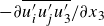 $-\partial \overline {u_i^{\prime}u_{\!j}^{\prime}u_3^{\prime}}/\partial x_3$
), which can be estimated from multilevel towers. Under the assumption of planar homogeneity, these vertical terms equal
$-\partial \overline {u_i^{\prime}u_{\!j}^{\prime}u_3^{\prime}}/\partial x_3$
), which can be estimated from multilevel towers. Under the assumption of planar homogeneity, these vertical terms equal $2T_{\textit{ij}}$
. In this work, therefore, instead of applying standard approaches to model
$2T_{\textit{ij}}$
. In this work, therefore, instead of applying standard approaches to model $T_{\textit{ij}}$
, these terms are estimated from tower measurements directly. In the same vein, the vertical pressure-transport term
$T_{\textit{ij}}$
, these terms are estimated from tower measurements directly. In the same vein, the vertical pressure-transport term $\varPi _{{ww}}^{\textit{tr}}$
can be evaluated directly from multilevel measurements of pressure (see M2HATS) or as a residual of the TKE budget (see § 3). Lastly, the Coriolis term (
$\varPi _{{ww}}^{\textit{tr}}$
can be evaluated directly from multilevel measurements of pressure (see M2HATS) or as a residual of the TKE budget (see § 3). Lastly, the Coriolis term ( $\textit{Co}$
) is commonly neglected in surface-layer studies due to its low magnitude near the ground (e.g. Stull Reference Stull1988; Kaimal & Finnigan Reference Kaimal and Finnigan1994, see § 5).
$\textit{Co}$
) is commonly neglected in surface-layer studies due to its low magnitude near the ground (e.g. Stull Reference Stull1988; Kaimal & Finnigan Reference Kaimal and Finnigan1994, see § 5).
2.2. Reduced model for energy anisotropy
While an important contribution to the anisotropy of the flow stems from the off-diagonal Reynolds stress tensor terms, i.e. momentum fluxes (cf. Stiperski et al. Reference Stiperski, Chamecki and Calaf2021a
), the focus here is on the anisotropy of the normal Reynolds stresses (i.e. velocity variances), as they provide information on the anisotropy in energy distribution. As a starting point, a reduced model for the Reynolds stresses (Bou-Zeid et al. Reference Bou-Zeid, Gao, Ansorge and Katul2018) is employed to examine the evolution of anisotropy with increasing instability. This model for half-variances assumes stationary, planar homogeneous conditions with no subsidence (all horizontal terms, as well as mean vertical advection are zero), with isotropic dissipation, negligible contribution from both turbulent ( $T_{\textit{ij}}$
) and pressure (
$T_{\textit{ij}}$
) and pressure ( $\varPi _{\textit{ij}}^{\textit{tr}}$
) transport terms, and pressure-strain correlations parametrised using only the standard linear Rotta closure (2.7), without the rapid terms related to isotropisation of the production. The latter allows writing the half-variance budgets in terms of velocity variance ratios (
$\varPi _{\textit{ij}}^{\textit{tr}}$
) transport terms, and pressure-strain correlations parametrised using only the standard linear Rotta closure (2.7), without the rapid terms related to isotropisation of the production. The latter allows writing the half-variance budgets in terms of velocity variance ratios ( $\overline {u_i^{\prime 2}}/e$
), which are functions of the TKE generating mechanisms – mechanical production (
$\overline {u_i^{\prime 2}}/e$
), which are functions of the TKE generating mechanisms – mechanical production ( $S_m = -\overline {u'w'}\partial {\overline {U}}/\partial z$
) and buoyancy production or damping (
$S_m = -\overline {u'w'}\partial {\overline {U}}/\partial z$
) and buoyancy production or damping ( $B = \overline {w'\theta _v^{\prime}}g/\overline {\theta }_{v0}$
) only. These componentwise velocity variance budgets are given by
$B = \overline {w'\theta _v^{\prime}}g/\overline {\theta }_{v0}$
) only. These componentwise velocity variance budgets are given by
 \begin{align} \frac {\overline {u^{\prime 2}}}{e} & = 2\frac {S_m}{c \varepsilon }\left ( \frac {2}{3} + \frac {1}{3} {\textit{Ri}}_{\!f} \right ) + \frac {2}{3}, \nonumber \\ \frac {\overline {v^{\prime 2}}}{e} & = 2\frac {S_m}{c \varepsilon }\left ( -\frac {1}{3} + \frac {1}{3} {\textit{Ri}}_{\!f} \right ) + \frac {2}{3}, \nonumber \\ \frac {\overline {w^{\prime 2}}}{e} & = 2\frac {S_m}{c \varepsilon }\left ( -\frac {1}{3} - \frac {2}{3} {\textit{Ri}}_{\!f} \right ) + \frac {2}{3}, \end{align}
where ${\textit{Ri}}_{\!f}=-B/S_m$
is the flux Richardson number, quantifying the relative importance of buoyancy forces over the mechanical production of TKE. Note that given that the Rotta model is formulated for the full variance budget, while the reduced model is developed for half-variances, a factor of 2 appears in the above equations, allowing the Rotta constant to maintain the value found in the rest of the literature. This factor is not used in Bou-Zeid et al. (Reference Bou-Zeid, Gao, Ansorge and Katul2018), where the Rotta constant is adjusted instead.
${\textit{Ri}}_{\!f}=-B/S_m$
is the flux Richardson number, quantifying the relative importance of buoyancy forces over the mechanical production of TKE. Note that given that the Rotta model is formulated for the full variance budget, while the reduced model is developed for half-variances, a factor of 2 appears in the above equations, allowing the Rotta constant to maintain the value found in the rest of the literature. This factor is not used in Bou-Zeid et al. (Reference Bou-Zeid, Gao, Ansorge and Katul2018), where the Rotta constant is adjusted instead.
The sum of the three velocity variances yields the TKE budget, which under the same assumptions can be simplified to a balance between molecular dissipation ( $\varepsilon$
), mechanical production (
$\varepsilon$
), mechanical production ( $S_m$
) and buoyancy (production or damping) (
$S_m$
) and buoyancy (production or damping) ( $B$
), i.e.
$B$
), i.e.
 \begin{equation} \frac {S_m}{\varepsilon } = \frac {1}{1 - {\textit{Ri}}_{\!f}}, \end{equation}
which allows the variance ratios to be expressed as a function of ${\textit{Ri}}_{\!f}$
only (Bou-Zeid et al. Reference Bou-Zeid, Gao, Ansorge and Katul2018). The full set of simplified equations are then given in dimensionless form by
${\textit{Ri}}_{\!f}$
only (Bou-Zeid et al. Reference Bou-Zeid, Gao, Ansorge and Katul2018). The full set of simplified equations are then given in dimensionless form by
 \begin{align} \frac {\overline {u^{\prime 2}}}{e} & = \frac {2}{3c }\left ( \frac {2 + {\textit{Ri}}_{\!f}}{1-{\textit{Ri}}_{\!f}} \right ) + \frac {2}{3}, \nonumber \\ \frac {\overline {v^{\prime 2}}}{e} & = \frac {2}{3c }\left ( \frac {-1 + {\textit{Ri}}_{\!f}}{1-{\textit{Ri}}_{\!f}}\right ) + \frac {2}{3}=\frac {2}{3}\left (1-\frac {1}{c}\right )\!, \nonumber \\ \frac {\overline {w^{\prime 2}}}{e} & = \frac {2}{3c}\left ( \frac {-1-2{\textit{Ri}}_{\!f}}{1-{\textit{Ri}}_{\!f}} \right ) + \frac {2}{3}. \end{align}
We refer to this model as model R (see table 1) and point out that for this model, $\overline {v^{\prime 2}}/{e}$
is constant and independent of
$\overline {v^{\prime 2}}/{e}$
is constant and independent of ${\textit{Ri}}_{\!f}$
. Moreover, the
${\textit{Ri}}_{\!f}$
. Moreover, the $\overline {v^{\prime 2}}/{e}$
model is realisable (i.e.
$\overline {v^{\prime 2}}/{e}$
model is realisable (i.e. $\overline {v^{\prime 2}}/{e}\gt 0$
) only when
$\overline {v^{\prime 2}}/{e}\gt 0$
) only when $c\gt 1$
. In both versions of this reduced model ((2.12) and (2.14)), the contribution of each variance to the total
$c\gt 1$
. In both versions of this reduced model ((2.12) and (2.14)), the contribution of each variance to the total $e$
is a result of the changing importance of production terms quantified through stratification (
$e$
is a result of the changing importance of production terms quantified through stratification ( ${\textit{Ri}}_{\!f}$
) on the one hand and the pressure redistribution on the other. It is through this later process that the less-energetic components receive energy from the energetic components at an equal rate, irrespective of stratification. This reduced model serves as a reference for assessing contributions from other anisotropy-generating mechanisms.
${\textit{Ri}}_{\!f}$
) on the one hand and the pressure redistribution on the other. It is through this later process that the less-energetic components receive energy from the energetic components at an equal rate, irrespective of stratification. This reduced model serves as a reference for assessing contributions from other anisotropy-generating mechanisms.
The versions of the models tested.

A feature of the reduced model is that the degree of anisotropy ( $y_B$
), defined based on the smallest eigenvalue (see (2.9)) is constant and is not a function of
$y_B$
), defined based on the smallest eigenvalue (see (2.9)) is constant and is not a function of ${\textit{Ri}}_{\!f}$
(figure 1). The reason lies in the fact that, without a contribution of momentum fluxes, the smallest eigenvalue equals the smallest component of
${\textit{Ri}}_{\!f}$
(figure 1). The reason lies in the fact that, without a contribution of momentum fluxes, the smallest eigenvalue equals the smallest component of $b_{\textit{ij}}$
, which is also the smallest variance ratio. Without a source of its own (shear or buoyancy) in the reduced budget, the smallest variance ratio in the entire
$b_{\textit{ij}}$
, which is also the smallest variance ratio. Without a source of its own (shear or buoyancy) in the reduced budget, the smallest variance ratio in the entire ${\textit{Ri}}_{\!f}\lt 0$
range is always the spanwise variance
${\textit{Ri}}_{\!f}\lt 0$
range is always the spanwise variance $\overline {v^{\prime 2}}/e$
(see figure 3 in Bou-Zeid et al. Reference Bou-Zeid, Gao, Ansorge and Katul2018), whose equation is independent of
$\overline {v^{\prime 2}}/e$
(see figure 3 in Bou-Zeid et al. Reference Bou-Zeid, Gao, Ansorge and Katul2018), whose equation is independent of ${\textit{Ri}}_{\!f}$
(2.14). The data in figure 1, however, suggest a significant influence of both stratification and height on the degree of anisotropy
${\textit{Ri}}_{\!f}$
(2.14). The data in figure 1, however, suggest a significant influence of both stratification and height on the degree of anisotropy $y_{B}$
, indicating a need for revisions to the reduced model to capture ASL anisotropy.
$y_{B}$
, indicating a need for revisions to the reduced model to capture ASL anisotropy.
Degree of energy anisotropy $y_{B}$
as a function of flux Richardson number
$y_{B}$
as a function of flux Richardson number ${\textit{Ri}}_{\!f}$
for the Cabauw tower data. Coloured points represent individual averaging periods for the four measurement heights (3 m in brown and 60–180 m in shades of blue), where the full coloured lines are the bin averages computed at logarithmically spaced
${\textit{Ri}}_{\!f}$
for the Cabauw tower data. Coloured points represent individual averaging periods for the four measurement heights (3 m in brown and 60–180 m in shades of blue), where the full coloured lines are the bin averages computed at logarithmically spaced ${\textit{Ri}}_{\!f}$
and shading is the interquartile range. The solid black line corresponds to the predictions of the reduced model R ((2.14) with
${\textit{Ri}}_{\!f}$
and shading is the interquartile range. The solid black line corresponds to the predictions of the reduced model R ((2.14) with $c = 1.8$
), while the dashed black curve corresponds to the prediction of the reduced model with adjusted Rotta constant (
$c = 1.8$
), while the dashed black curve corresponds to the prediction of the reduced model with adjusted Rotta constant ( $c = 6.3$
) and added wall blocking
$c = 6.3$
) and added wall blocking $(a_u,a_v,a_w) = (1.14, 1.13, 0.73)$
(model Ra).
$(a_u,a_v,a_w) = (1.14, 1.13, 0.73)$
(model Ra).

2.3. Revisions to the reduced model for energy anisotropy
The model in (2.14) can be expanded in multiple ways to accommodate different sources of anisotropy. A process missing from the classic Rotta model is the existence of wall effects (or ‘pressure echo’) due to the rigid boundary (Pope Reference Pope2000; McColl et al. Reference McColl, Katul, Gentine and Entekhabi2016), disproportionately affecting the wall-normal variance $\overline {w^{\prime 2}}$
. This source of anisotropy can be added to the Rotta closure itself by allowing the energetics of individual velocity components not to strive towards a state of equipartition. Instead, a state that ‘arrests’ a certain degree of anisotropy due to the wall is proposed, where the modified Rotta closure can be expressed as
$\overline {w^{\prime 2}}$
. This source of anisotropy can be added to the Rotta closure itself by allowing the energetics of individual velocity components not to strive towards a state of equipartition. Instead, a state that ‘arrests’ a certain degree of anisotropy due to the wall is proposed, where the modified Rotta closure can be expressed as
 \begin{equation} \varPi _{\textit{ij}}^S = -\frac {c\varepsilon }{e}\left (\overline {u^{\prime}_{i}u^{\prime}_{\!j}} - \frac {2}{3}e \delta _{\textit{ij}} \, a_i \right ). \end{equation}
Here no summation in $i$
in the second term on the right-hand side is intended. The coefficients
$i$
in the second term on the right-hand side is intended. The coefficients $a_i$
(or
$a_i$
(or $a_1=a_u$
,
$a_1=a_u$
, $a_2=a_v$
and
$a_2=a_v$
and $a_3=a_w$
) are required to be positive, and to satisfy
$a_3=a_w$
) are required to be positive, and to satisfy $a_1 + a_2 + a_3 = 3$
, in order for the summed redistribution terms not to produce or dissipate TKE. This is the essence of the wall-function corrections to the pressure-strain interaction. In this case the variance equations become
$a_1 + a_2 + a_3 = 3$
, in order for the summed redistribution terms not to produce or dissipate TKE. This is the essence of the wall-function corrections to the pressure-strain interaction. In this case the variance equations become
 \begin{align} \frac {\overline {u^{\prime 2}}}{e} & = \frac {2}{3c }\left ( \frac {2 + {\textit{Ri}}_{\!f}}{1-{\textit{Ri}}_{\!f}} \right ) + \frac {2}{3}a_u, \nonumber \\ \frac {\overline {v^{\prime 2}}}{e} & = \frac {2}{3c }\left ( \frac {-1 + {\textit{Ri}}_{\!f}}{1-{\textit{Ri}}_{\!f}}\right ) + \frac {2}{3}a_v= -\frac {2}{3c } + \frac {2}{3}a_v, \nonumber \\ \frac {\overline {w^{\prime 2}}}{e} & = \frac {2}{3c}\left ( \frac {-1-2{\textit{Ri}}_{\!f}}{1-{\textit{Ri}}_{\!f}} \right ) + \frac {2}{3}a_w. \end{align}
We refer to this model as model Ra (see table 1). Note that if $a_w$
is sufficiently small and, thus,
$a_w$
is sufficiently small and, thus, $\overline {w^{\prime 2}}/e$
becomes the smallest variance ratio, this model allows the degree of anisotropy to vary with stratification (see figure 1, dashed line). This criterion is regularly satisfied in ASL, where even at 180 m the wall-normal variance is routinely found to be the smallest one (see Stiperski et al. Reference Stiperski, Calaf and Rotach2019).
$\overline {w^{\prime 2}}/e$
becomes the smallest variance ratio, this model allows the degree of anisotropy to vary with stratification (see figure 1, dashed line). This criterion is regularly satisfied in ASL, where even at 180 m the wall-normal variance is routinely found to be the smallest one (see Stiperski et al. Reference Stiperski, Calaf and Rotach2019).
Beyond wall-blocking effects, another source of anisotropy in the ASL is the anisotropy of TKE dissipation rate. Generally, in high-Reynolds-number flows, micro-scale eddies are assumed to be isotropic (Kolmogorov Reference Kolmogorov1941), and this assumption is employed in the reduced model. The assumption of dissipation isotropy is, however, not guaranteed in realistic ASL flows or generally close to the wall (e.g. Biltoft Reference Biltoft2001). The inclusion of dissipation anisotropy would modify the constants in the first term on the right-hand side of (2.16) (cf. Appendix C), and would thus only affect the magnitude of the Rotta constant. To accommodate this effect here, the Rotta constants $c_i$
in all explored models are allowed to vary between the velocity components as suggested by previous studies (see Heinze et al. Reference Heinze, Mironov and Raasch2016; Yi et al. Reference Yi, Koseff and Bou-Zeid2025).
$c_i$
in all explored models are allowed to vary between the velocity components as suggested by previous studies (see Heinze et al. Reference Heinze, Mironov and Raasch2016; Yi et al. Reference Yi, Koseff and Bou-Zeid2025).
Next, the role of the rapid return-to-isotropy terms neglected in the reduced model can also be added. These include the isotropisation of production terms due to shear, vorticity and buoyancy ((2.10)–(2.11), table 3 in Appendix A):
 \begin{align} \frac {\overline {u^{\prime 2}}}{e} & = \frac {2}{c_u \varepsilon } \left [ \left ( \frac {2}{3} + \frac {1}{3} {\textit{Ri}}_{\!f} \right )S_m + \frac {1}{3}C_{B}^uB - \left (\frac {1}{3} C^u_{S1} + C^u_{S2} \right )\frac {S_m}{2} \right ]+ \frac {2}{3}a_u, \nonumber \\ \frac {\overline {v^{\prime 2}}}{e} & = \frac {2}{c_v \varepsilon } \left [ \left ( -\frac {1}{3} + \frac {1}{3} {\textit{Ri}}_{\!f} \right )S_m + \frac {1}{3}C_{B}^uB + \frac {2}{3}C^u_{S1}\frac {S_m}{2}\right ] + \frac {2}{3}a_v, \nonumber \\ \frac {\overline {w^{\prime 2}}}{e} &= \frac {2}{c_w \varepsilon } \left [ \left ( -\frac {1}{3} - \frac {2}{3} {\textit{Ri}}_{\!f} \right )S_m - \frac {2}{3}C_{B}^u B - \left (\frac {1}{3} C^u_{S1} - C^u_{S2} \right )\frac {S_m}{2} \right ] + \frac {2}{3}a_w. \end{align}
This model will be referred to as model E, where E stands for extended (see table 1).
Finally, turbulent transport terms $T_{\textit{ij}}$
, known to be relevant in buoyancy-driven conditions (e.g. Lin Reference Lin2000; Stiperski et al. Reference Stiperski, Chamecki and Calaf2021a
), can be added to the reduced model (Bou-Zeid et al. Reference Bou-Zeid, Gao, Ansorge and Katul2018, cf. their Appendix A). Allowing for transport in this modelling framework was shown to be critical for explaining turbulence levels under stable conditions at heights where the local dissipation plus buoyant destruction exceeded shear production (Freire, Dias & Chamecki Reference Freire, Dias and Chamecki2019). Under the assumption of planar homogeneity, only the vertical turbulence transport terms are relevant for extending the reduced model. In case transport is included, however, the balance between production and dissipation mechanisms encoded in (2.13) no longer holds, and the full form of the budget equations (2.12) must be used. Still, the dissipation is maintained to be isotropic. Additionally, the vertical pressure-transport term (
$T_{\textit{ij}}$
, known to be relevant in buoyancy-driven conditions (e.g. Lin Reference Lin2000; Stiperski et al. Reference Stiperski, Chamecki and Calaf2021a
), can be added to the reduced model (Bou-Zeid et al. Reference Bou-Zeid, Gao, Ansorge and Katul2018, cf. their Appendix A). Allowing for transport in this modelling framework was shown to be critical for explaining turbulence levels under stable conditions at heights where the local dissipation plus buoyant destruction exceeded shear production (Freire, Dias & Chamecki Reference Freire, Dias and Chamecki2019). Under the assumption of planar homogeneity, only the vertical turbulence transport terms are relevant for extending the reduced model. In case transport is included, however, the balance between production and dissipation mechanisms encoded in (2.13) no longer holds, and the full form of the budget equations (2.12) must be used. Still, the dissipation is maintained to be isotropic. Additionally, the vertical pressure-transport term ( $\varPi _{{ww}}^{\textit{tr}}$
) can also be included if its contribution can be estimated from the data. Most measurement campaigns, however, do not include barometers measuring at sufficient temporal resolution with an adequate frequency response, and therefore, do not allow its direct estimation. The effect of this term on anisotropy is discussed later on in § 4.3.
$\varPi _{{ww}}^{\textit{tr}}$
) can also be included if its contribution can be estimated from the data. Most measurement campaigns, however, do not include barometers measuring at sufficient temporal resolution with an adequate frequency response, and therefore, do not allow its direct estimation. The effect of this term on anisotropy is discussed later on in § 4.3.
The final model accommodating all these revisions is given by
 \begin{align} \begin{split} \frac {\overline {u^{\prime 2}}}{e} &= \frac {2}{c_u \varepsilon } \bigg [ \left ( \frac {2}{3} + \frac {1}{3} {\textit{Ri}}_{\!f} \right )S_m + \frac {1}{3}C_{B}^uB \\ &\quad - \left (\frac {1}{3} C^u_{S1} + C^u_{S2} \right )\frac {S_m}{2} + \frac {\left ( T_{{ww}}+ T_{{vv}} -2T_{\textit{uu}} + \varPi _{{ww}}^{\textit{tr}} \right )}{3} \bigg ]+ \frac {2}{3}a_u, \end{split} \nonumber \\ \begin{split} \frac {\overline {v^{\prime 2}}}{e} &= \frac {2}{c_v \varepsilon } \bigg [ \left ( -\frac {1}{3} + \frac {1}{3} {\textit{Ri}}_{\!f} \right )S_m + \frac {1}{3}C_{B}^uB \\ &\quad + \frac {2}{3}C^u_{S1}\frac {S_m}{2} + \frac {\left (T_{{ww}} +T_{\textit{uu}} -2T_{{vv}} + \varPi _{{ww}}^{\textit{tr}} \right )}{3} \bigg ] + \frac {2}{3}a_v, \end{split} \nonumber \\ \begin{split} \frac {\overline {w^{\prime 2}}}{e} &= \frac {2}{c_w \varepsilon } \bigg [ \left ( -\frac {1}{3} - \frac {2}{3} {\textit{Ri}}_{\!f} \right )S_m - \frac {2}{3}C_{B}^u B \\ &\quad - \left (\frac {1}{3} C^u_{S1} - C^u_{S2} \right )\frac {S_m}{2} + \frac {\left ( T_{\textit{uu}} + T_{{vv}} -2T_{{ww}} - 2\varPi _{{ww}}^{\textit{tr}} \right )}{3} \bigg ] + \frac {2}{3}a_w. \end{split} \end{align}
Here $T_{\textit{uu}}$
(or
$T_{\textit{uu}}$
(or $T_{11}$
),
$T_{11}$
), $T_{{vv}}$
(or
$T_{{vv}}$
(or $T_{22}$
) and
$T_{22}$
) and $T_{{ww}}$
(or
$T_{{ww}}$
(or $T_{33}$
) are the vertical transport terms of the respective half-variance (
$T_{33}$
) are the vertical transport terms of the respective half-variance ( $T_{\textit{ii}} = -(1/2)\partial {\overline {w'u_i^{\prime 2}}}/\partial {z}$
), with no summation intended. This model will be referred to as model Et if only turbulent transport terms
$T_{\textit{ii}} = -(1/2)\partial {\overline {w'u_i^{\prime 2}}}/\partial {z}$
), with no summation intended. This model will be referred to as model Et if only turbulent transport terms $T_{\textit{ii}}$
are considered, or as model Etp if pressure transport
$T_{\textit{ii}}$
are considered, or as model Etp if pressure transport $\varPi _{{ww}}^{\textit{tr}}$
is also taken into account (see table 1).
$\varPi _{{ww}}^{\textit{tr}}$
is also taken into account (see table 1).
An earlier study noted that the contribution of the transport terms to the non-dimensional variances depends on whether the individual transport components act together or against each other (Bou-Zeid et al. Reference Bou-Zeid, Gao, Ansorge and Katul2018). Expressing the transport of TKE as $T_e= T_{\textit{uu}} + T_{{vv}} +T_{{ww}}$
, the transport contribution for a given component
$T_e= T_{\textit{uu}} + T_{{vv}} +T_{{ww}}$
, the transport contribution for a given component $i$
can be expressed as
$i$
can be expressed as $T_e-3T_{\textit{ii}}$
(cf. (2.18)). Since the vertical turbulent transport in the near-surface region of the convective boundary layer commonly carries a negative sign and is a loss term (
$T_e-3T_{\textit{ii}}$
(cf. (2.18)). Since the vertical turbulent transport in the near-surface region of the convective boundary layer commonly carries a negative sign and is a loss term ( $e$
is exported from ASL into the mixed layer), these transport terms are all expected to be negative (this indeed was found to hold except under very stable stratification by Freire et al. Reference Freire, Dias and Chamecki2019). If the component
$e$
is exported from ASL into the mixed layer), these transport terms are all expected to be negative (this indeed was found to hold except under very stable stratification by Freire et al. Reference Freire, Dias and Chamecki2019). If the component $i$
is the least energetic, it will most likely result in a weaker negative transport than the other terms, and thus,
$i$
is the least energetic, it will most likely result in a weaker negative transport than the other terms, and thus, $T_e-3T_{\textit{ii}}\lt 0$
(again supported by the results of Freire et al. Reference Freire, Dias and Chamecki2019 that indicated that
$T_e-3T_{\textit{ii}}\lt 0$
(again supported by the results of Freire et al. Reference Freire, Dias and Chamecki2019 that indicated that $T_{{ww}}\approx 0.28T_e$
), while for the most energetic component, we expect
$T_{{ww}}\approx 0.28T_e$
), while for the most energetic component, we expect $T_e-3T_{\textit{ii}}\gt 0$
. Therefore, the contribution of the net transport terms boosts the most energetic component relative to the least energetic, and acts against the return-to-isotropy process.
$T_e-3T_{\textit{ii}}\gt 0$
. Therefore, the contribution of the net transport terms boosts the most energetic component relative to the least energetic, and acts against the return-to-isotropy process.
The final model has a number of parameters that need to be externally supplied. Unless otherwise specified, the rapid term constants are set to $C^u_{B} = C^u_{S1} = C^u_{S2} = 3/5$
(Gibson & Launder Reference Gibson and Launder1978; Heinze et al. Reference Heinze, Mironov and Raasch2016). The constant
$C^u_{B} = C^u_{S1} = C^u_{S2} = 3/5$
(Gibson & Launder Reference Gibson and Launder1978; Heinze et al. Reference Heinze, Mironov and Raasch2016). The constant $c$
in the Rotta model has to be different in case the full models E and Etp ((2.17)–(2.18)) are used or if only the slow (i.e. Rotta) terms are kept (2.14 and 2.16, models R and Ra). In the full model, it was reported that values between 1 and 3 (and possibly centred at 1) are plausible (Heinze et al. Reference Heinze, Mironov and Raasch2016); however, when approximating the return to isotropy using the slow part only,
$c$
in the Rotta model has to be different in case the full models E and Etp ((2.17)–(2.18)) are used or if only the slow (i.e. Rotta) terms are kept (2.14 and 2.16, models R and Ra). In the full model, it was reported that values between 1 and 3 (and possibly centred at 1) are plausible (Heinze et al. Reference Heinze, Mironov and Raasch2016); however, when approximating the return to isotropy using the slow part only, $c=1.8$
(Pope Reference Pope2000; Bou-Zeid et al. Reference Bou-Zeid, Gao, Ansorge and Katul2018).
$c=1.8$
(Pope Reference Pope2000; Bou-Zeid et al. Reference Bou-Zeid, Gao, Ansorge and Katul2018).
2.4. Nonlinear Rotta closures
Apart from the modifications introduced to the Rotta closure in the previous subsection (cf. (2.15)), a number of alternative nonlinear and anisotropic slow pressure-strain models exist that include the anisotropy invariants to the closure directly (e.g. Chung & Kim Reference Chung and Kim1995; Choi & Lumley Reference Choi and Lumley2001; Warrior et al. Reference Warrior, Mathews, Maity and Sasmal2014). Here, the performance of two formulations is explored. The Speziale et al. (Reference Speziale, Sarkar and Gatski1991) nonlinear model has shown superior performance to the classic Rotta type closures for engineering neutral flows (e.g. Alfonsi Reference Alfonsi2009; Homan et al. Reference Homan, Shende and Mani2024; Liu et al. Reference Liu, Ahmed and Chakraborty2024):
 \begin{equation} \varPi _{\textit{ij}}^S = -\frac {C_1}{2}\varepsilon b_{\textit{ij}} + \frac {C_2}{4}\varepsilon \left (b_{\textit{ik}}b_{\textit{kj}} -\frac {1}{3}b_{\textit{mn}}b_{\textit{nm}}\delta _{\textit{ij}} \right ) + a_{i_{\textit{SSG}}}. \end{equation}
This equation has been modified compared with Speziale et al. (Reference Speziale, Sarkar and Gatski1991) to account for the difference in definition of the anisotropy tensor $b_{\textit{ij}}$
in the study here (it equals twice the anisotropy tensor in the original study), as well as to account for the existence of wall effects, as done for the Rotta model in the previous section through the wall constants
$b_{\textit{ij}}$
in the study here (it equals twice the anisotropy tensor in the original study), as well as to account for the existence of wall effects, as done for the Rotta model in the previous section through the wall constants $a_{i_{\textit{SSG}}}$
. The constants
$a_{i_{\textit{SSG}}}$
. The constants $C_{1} = 3.4$
and
$C_{1} = 3.4$
and $C_{2} = 4.2$
are given in Speziale et al. (Reference Speziale, Sarkar and Gatski1991). This model will be referred to with the subscript
$C_{2} = 4.2$
are given in Speziale et al. (Reference Speziale, Sarkar and Gatski1991). This model will be referred to with the subscript $SSG$
(table 1).
$SSG$
(table 1).
The nonlinear model proposed by Craft et al. (Reference Craft, Ince and Launder1996) and used in Heinze et al. (Reference Heinze, Mironov and Raasch2016) has been developed for flows affected by buoyancy:
 \begin{equation} \varPi _{\textit{ij}}^S = -C_{T1}^u\varepsilon \left [b_{\textit{ij}} + C_{T2}^u\left (b_{\textit{ik}}b_{\textit{kj}} -\frac {1}{3}A_2\delta _{\textit{ij}} \right ) \right ] + a_{i_{\textit{TLC}}}. \end{equation}
Here $C_{T1}^u = (3.75 A_2^{1/2} + 1 )A$
,
$C_{T1}^u = (3.75 A_2^{1/2} + 1 )A$
, $C_{T2}^u = 0.7$
, while
$C_{T2}^u = 0.7$
, while $A_2 = b_{\textit{mn}}b_{\textit{nm}}$
and
$A_2 = b_{\textit{mn}}b_{\textit{nm}}$
and $A_3 = b_{lm}b_{\textit{mn}}b_{nl}$
are the invariants of
$A_3 = b_{lm}b_{\textit{mn}}b_{nl}$
are the invariants of $ b_{\textit{ij}} $
and form the flatness parameter
$ b_{\textit{ij}} $
and form the flatness parameter $A = 1 - {(9/8)} (A_2 - A_3 )$
. Note that both in the original publication of Craft et al. (Reference Craft, Ince and Launder1996) and in Heinze et al. (Reference Heinze, Mironov and Raasch2016) the indices in
$A = 1 - {(9/8)} (A_2 - A_3 )$
. Note that both in the original publication of Craft et al. (Reference Craft, Ince and Launder1996) and in Heinze et al. (Reference Heinze, Mironov and Raasch2016) the indices in $A_2$
and
$A_2$
and $A_3$
are incorrectly specified, leading to a model that does not sum to zero. The factor
$A_3$
are incorrectly specified, leading to a model that does not sum to zero. The factor $a_{i_{\textit{TLC}}}$
is again added to account for wall effects. This model will be referred to with the subscript
$a_{i_{\textit{TLC}}}$
is again added to account for wall effects. This model will be referred to with the subscript $TLC$
(table 1).
$TLC$
(table 1).
3. Data and methods
3.1. Datasets and turbulence data post-processing
A number of datasets representative of mostly flat and horizontally homogeneous (i.e. canonical) terrain are employed. These datasets are the vertical tower in the AHATS (Nguyen et al. Reference Nguyen, Horst, Oncley and Tong2013) experiment, the Cabauw tower (Beljaars & Bosveld Reference Beljaars and Bosveld1997), NEAR tower from the METCRAX II experiment (Lehner et al. Reference Lehner2016) and the t0 tower from the M2HATS campaign (Tong et al. Reference Tong2026). M2HATS stands out as the dataset where in addition to sonic anemometers, the nano-barometers (Digiquartz Paroscientific 6000 measuring at 20 Hz) were installed at each observational level, allowing a direct estimation of the vertical pressure-transport term. Characteristics of individual datasets are summarised in table 2. Due to a lack of direct observations, the boundary layer height for the METCRAX II experiment was obtained from the ERA5 reanalysis (Hersbach et al. Reference Hersbach2020).
Information on the datasets used in the study.

Turbulence time series from the different datasets and sites were processed using a uniform procedure described in prior studies (Stiperski & Calaf Reference Stiperski and Calaf2018; Stiperski et al. Reference Stiperski, Calaf and Rotach2019, Reference Stiperski, Chamecki and Calaf2021a , Reference Stiperski, Katul and Calafb ; Stiperski & Calaf Reference Stiperski and Calaf2023). Turbulence statistics were computed over 30 min block averages, with prior linear detrending. The 30 min average is the standard processing time in atmospheric turbulence studies (e.g. Aubinet, Vesala & Papale Reference Aubinet, Vesala and Papale2012) and ensures that the largest convective eddies are represented in the temporal mean, while eliminating the non-turbulent signals and the influence of the daily cycle (i.e. non-stationarity). Using a 1 h averaging time had no substantial influence on the results (not shown).
Data were rotated into the streamline coordinates using a double rotation procedure (Aubinet et al. Reference Aubinet, Vesala and Papale2012) in which the mean spanwise ( $\overline {V}$
) and wall-normal (
$\overline {V}$
) and wall-normal ( $\overline {W}$
) velocity components over each 30 min period are set to zero, and the streamwise direction (
$\overline {W}$
) velocity components over each 30 min period are set to zero, and the streamwise direction ( $\overline {U}$
) is aligned with the mean wind direction.
$\overline {U}$
) is aligned with the mean wind direction.
Data were quality controlled for instrument errors and for values outside of the physical range, as well as for wind directions influenced by the tower structure. Additionally, only periods for which the spectral slope of the streamwise and spanwise spectra in the inertial subrange equalled $-5/3$
with a
$-5/3$
with a $20\,\%$
error margin, and for which the stationarity of the mean wind speed was limited to
$20\,\%$
error margin, and for which the stationarity of the mean wind speed was limited to $30\,\%$
based on the common stationarity test of Foken & Wichura (Reference Foken and Wichura1996), were retained. A more stringent criterion on the spectral slope (e.g.
$30\,\%$
based on the common stationarity test of Foken & Wichura (Reference Foken and Wichura1996), were retained. A more stringent criterion on the spectral slope (e.g. $10\,\%)$
yielded no significant differences to the results. No additional quality criteria were applied to the data (e.g. stationarity of higher-order statistics).
$10\,\%)$
yielded no significant differences to the results. No additional quality criteria were applied to the data (e.g. stationarity of higher-order statistics).
Finally, only the unstable daytime surface layer was explored. The buoyancy flux ( $\overline {w'\theta _v^{\prime}}$
, where
$\overline {w'\theta _v^{\prime}}$
, where $\theta _v$
was taken to equal the sonic temperature) was therefore required to be positive at all observational heights. This criterion prevented the misclassification of transition periods (morning and evening) or nighttime counter-gradient fluxes as daytime unstably stratified turbulence.
$\theta _v$
was taken to equal the sonic temperature) was therefore required to be positive at all observational heights. This criterion prevented the misclassification of transition periods (morning and evening) or nighttime counter-gradient fluxes as daytime unstably stratified turbulence.
3.2. Computation of the Reynolds budgets terms
The Reynolds stress budget terms were evaluated at each observational height. The vertical wind shear, as part of the shear production term ( $S_m$
) was obtained by fitting the function
$S_m$
) was obtained by fitting the function $a + b\,z + c\,\ln {z}$
through the mean velocity profile
$a + b\,z + c\,\ln {z}$
through the mean velocity profile $\overline {U}(z)$
, and evaluating the gradient analytically.
$\overline {U}(z)$
, and evaluating the gradient analytically.
Vertical components of the turbulence transport $T_{\textit{ii}} = -(1/2)\partial {\overline {w'u_i^{\prime 2}}}/\partial {z}$
were computed by fitting a polynomial of the form
$T_{\textit{ii}} = -(1/2)\partial {\overline {w'u_i^{\prime 2}}}/\partial {z}$
were computed by fitting a polynomial of the form $a + b\,z + c\,z^2 + d\,\ln {z}$
through the triple correlation terms (
$a + b\,z + c\,z^2 + d\,\ln {z}$
through the triple correlation terms ( $\overline {w'u_i^{\prime 2}}$
) and analytically evaluating the gradient. If the shape of the profile could not be captured with this function, a simpler second or third degree polynomial in
$\overline {w'u_i^{\prime 2}}$
) and analytically evaluating the gradient. If the shape of the profile could not be captured with this function, a simpler second or third degree polynomial in $z$
was explored instead. The form that produced the smallest root-mean-square fitting error was chosen for each averaging period for gradient evaluations.
$z$
was explored instead. The form that produced the smallest root-mean-square fitting error was chosen for each averaging period for gradient evaluations.
The vertical pressure-transport term $\varPi _{{ww}}^{\textit{tr}}$
was estimated as a residual of the TKE budget for all the datasets, while the pressure-strain term for each of the velocity components
$\varPi _{{ww}}^{\textit{tr}}$
was estimated as a residual of the TKE budget for all the datasets, while the pressure-strain term for each of the velocity components $\varPi _{\textit{ii}}^{\textit{str}}$
(in figures 6 and 9) was estimated as the residual of the respective variance budget. In M2HATS, however, the vertical pressure-transport term was also computed directly from the pressure-covariance observations. For this purpose, the turbulent pressure signal was first filtered using a moving-average window with an 8 min window size (corresponding to approximately 15 min high pass filter, significantly larger than the integral time scale of the streamwise velocity component) to eliminate the sources of low-frequency contaminations (e.g. Aslan, Katul & Aurela Reference Aslan, Katul and Aurela2025). The covariance between the vertical velocity and filtered pressure signal was computed for each averaging window. The pressure transport was then calculated by fitting the function
$\varPi _{\textit{ii}}^{\textit{str}}$
(in figures 6 and 9) was estimated as the residual of the respective variance budget. In M2HATS, however, the vertical pressure-transport term was also computed directly from the pressure-covariance observations. For this purpose, the turbulent pressure signal was first filtered using a moving-average window with an 8 min window size (corresponding to approximately 15 min high pass filter, significantly larger than the integral time scale of the streamwise velocity component) to eliminate the sources of low-frequency contaminations (e.g. Aslan, Katul & Aurela Reference Aslan, Katul and Aurela2025). The covariance between the vertical velocity and filtered pressure signal was computed for each averaging window. The pressure transport was then calculated by fitting the function $ a + b\,z + c\,z^2+d\,\ln {z}$
through
$ a + b\,z + c\,z^2+d\,\ln {z}$
through $\overline {w'p'}(z)$
at eight observational heights, and evaluating the gradient analytically. The high pass filtering of pressure observations resulted in a significantly better match with the vertical pressure-transport estimates as the residual of the TKE budget than if the pressure observations were not filtered. Given the uncertainty in the behaviour of the triple moments and the pressure–velocity correlations with height, these fitting procedures are a source of non-negligible uncertainty in the estimated turbulent and pressure-transport terms, and therefore, also Reynolds stress budgets.
$\overline {w'p'}(z)$
at eight observational heights, and evaluating the gradient analytically. The high pass filtering of pressure observations resulted in a significantly better match with the vertical pressure-transport estimates as the residual of the TKE budget than if the pressure observations were not filtered. Given the uncertainty in the behaviour of the triple moments and the pressure–velocity correlations with height, these fitting procedures are a source of non-negligible uncertainty in the estimated turbulent and pressure-transport terms, and therefore, also Reynolds stress budgets.
The TKE dissipation rate ( $\varepsilon$
) was determined from the inertial subrange of the 30 min spectra of the streamwise velocity component, following the inertial dissipation method (Chamecki & Dias Reference Chamecki and Dias2004):
$\varepsilon$
) was determined from the inertial subrange of the 30 min spectra of the streamwise velocity component, following the inertial dissipation method (Chamecki & Dias Reference Chamecki and Dias2004):
 \begin{equation} S_u = \alpha _uk^{-5/3}\varepsilon ^{2/3}. \end{equation}
Here $S_u$
is the streamwise power spectral density,
$S_u$
is the streamwise power spectral density, $k=(2\pi f)/\overline {U}$
is the streamwise wavenumber determined based on Taylor’s hypothesis,
$k=(2\pi f)/\overline {U}$
is the streamwise wavenumber determined based on Taylor’s hypothesis, $f$
the frequency and
$f$
the frequency and $\alpha _u = {18/55} \, C_e$
, where
$\alpha _u = {18/55} \, C_e$
, where $C_e = 1.5$
is the Kolmogorov constant for the streamwise component. To ensure that the TKE dissipation rate is representative of the inertial subrange and to avoid aliasing at high frequencies, the frequency range over which
$C_e = 1.5$
is the Kolmogorov constant for the streamwise component. To ensure that the TKE dissipation rate is representative of the inertial subrange and to avoid aliasing at high frequencies, the frequency range over which $\varepsilon$
was estimated was limited between the frequency corresponding to the peak in the premultiplied wall-normal velocity spectrum at frequencies corresponding to
$\varepsilon$
was estimated was limited between the frequency corresponding to the peak in the premultiplied wall-normal velocity spectrum at frequencies corresponding to $k z\gt 1$
on the one hand and
$k z\gt 1$
on the one hand and $f=10^{-0.1}$
on the other. The spectra were smoothed prior to computing the dissipation rate by computing bin averages of spectral density within logarithmically spaced bins in the frequency space. Finally, the TKE dissipation rate for each averaging period was computed as the median of the dissipation rate estimates at each frequency within the inertial subrange to allow a robust estimate of dissipation. Additionally, the spectral slope of the inertial subrange was estimated from the smoothed spectra using robust linear regression in log–log space (MATLAB function robustfit with the Tukey bisquare estimator; see DuMouchel & O’Brien 1989), and used as a quality criterion for the computed TKE dissipation.
$f=10^{-0.1}$
on the other. The spectra were smoothed prior to computing the dissipation rate by computing bin averages of spectral density within logarithmically spaced bins in the frequency space. Finally, the TKE dissipation rate for each averaging period was computed as the median of the dissipation rate estimates at each frequency within the inertial subrange to allow a robust estimate of dissipation. Additionally, the spectral slope of the inertial subrange was estimated from the smoothed spectra using robust linear regression in log–log space (MATLAB function robustfit with the Tukey bisquare estimator; see DuMouchel & O’Brien 1989), and used as a quality criterion for the computed TKE dissipation.
It has been known for quite some time now that while the scaling laws (i.e. $k^{-5/3}$
) are robust to the local isotropy assumption, the spectral ratios that determine the Kolmogorov constants for each velocity component are not (Saddoughi & Veeravalli Reference Saddoughi and Veeravalli1994; Hsieh & Katul Reference Hsieh and Katul1997) as they may be impacted by turbulent intensity and intermittency, thus requiring corrections. The estimated dissipation rates were therefore multiplied by the turbulence intensity correction factor
$k^{-5/3}$
) are robust to the local isotropy assumption, the spectral ratios that determine the Kolmogorov constants for each velocity component are not (Saddoughi & Veeravalli Reference Saddoughi and Veeravalli1994; Hsieh & Katul Reference Hsieh and Katul1997) as they may be impacted by turbulent intensity and intermittency, thus requiring corrections. The estimated dissipation rates were therefore multiplied by the turbulence intensity correction factor $F_u$
for the streamwise component (
$F_u$
for the streamwise component ( $F_u = 1+(11/9)I_u^2$
), where
$F_u = 1+(11/9)I_u^2$
), where $I_u = \sqrt {\overline {u^{\prime 2}}}/\overline {U}$
is the turbulence intensity, following Hsieh & Katul (Reference Hsieh and Katul1997). In addition, the non-orthogonal design of the majority of sonic anemometers used in the study has been shown to impact the wall-normal velocity and would require corrections for transducer shadowing (Horst, Semmer & Maclean Reference Horst, Semmer and Maclean2015; Frank et al. Reference Frank, Massman, Swiatek, Zimmerman and Ewers2016; Peña et al. Reference Peña, Dellwik and Mann2019). This correction, however, has not been implemented here as it would require access to the fully raw sonic anemometer signal.
$I_u = \sqrt {\overline {u^{\prime 2}}}/\overline {U}$
is the turbulence intensity, following Hsieh & Katul (Reference Hsieh and Katul1997). In addition, the non-orthogonal design of the majority of sonic anemometers used in the study has been shown to impact the wall-normal velocity and would require corrections for transducer shadowing (Horst, Semmer & Maclean Reference Horst, Semmer and Maclean2015; Frank et al. Reference Frank, Massman, Swiatek, Zimmerman and Ewers2016; Peña et al. Reference Peña, Dellwik and Mann2019). This correction, however, has not been implemented here as it would require access to the fully raw sonic anemometer signal.
The Eulerian integral length scales of the streamwise and wall-normal velocity components ( $\lambda _u,\lambda _w$
) were estimated from the autocorrelation function of the respective velocity component. Here, first the integral time scale was determined as the integral of the autocorrelation function until the first zero crossing and then subsequently converted to the integral length scale through Taylor’s hypothesis. The impact of this choice of computing the integral time scale compared with the more commonly applied computation as the time scale at which the autocorrelation function drops to
$\lambda _u,\lambda _w$
) were estimated from the autocorrelation function of the respective velocity component. Here, first the integral time scale was determined as the integral of the autocorrelation function until the first zero crossing and then subsequently converted to the integral length scale through Taylor’s hypothesis. The impact of this choice of computing the integral time scale compared with the more commonly applied computation as the time scale at which the autocorrelation function drops to $e^{-1}$
, where
$e^{-1}$
, where $e$
is the base of the natural logarithm (Kaimal & Finnigan Reference Kaimal and Finnigan1994) is discussed in the supplemental material available at https://doi.org/10.1017/jfm.2026.11761.
$e$
is the base of the natural logarithm (Kaimal & Finnigan Reference Kaimal and Finnigan1994) is discussed in the supplemental material available at https://doi.org/10.1017/jfm.2026.11761.
The inclination angles of coherent structures in the streamwise $\beta _u$
(spanwise
$\beta _u$
(spanwise $\beta _v$
) direction were computed following Chauhan et al. (Reference Chauhan, Hutchins, Monty and Marusic2013). In each averaging window and for each observational level, the two-point correlation was computed between streamwise (spanwise) velocity fluctuations at the lowest observational level and any successive level. The observed peak in the two-point correlation (
$\beta _v$
) direction were computed following Chauhan et al. (Reference Chauhan, Hutchins, Monty and Marusic2013). In each averaging window and for each observational level, the two-point correlation was computed between streamwise (spanwise) velocity fluctuations at the lowest observational level and any successive level. The observed peak in the two-point correlation ( $\Delta t_{u,v}$
) was associated with a horizontal shift (
$\Delta t_{u,v}$
) was associated with a horizontal shift ( $\Delta x_{u,v}$
) through Taylor’s hypothesis (
$\Delta x_{u,v}$
) through Taylor’s hypothesis ( $\Delta x=\overline {U} \Delta t$
). The inclination angle was then computed as
$\Delta x=\overline {U} \Delta t$
). The inclination angle was then computed as
 \begin{equation} \beta _{u,v} = \arctan \left (\frac {\Delta x_{u,v}}{\Delta z}\right )\!, \end{equation}
where $\Delta z$
indicates the distance between the first and any successive observational level.
$\Delta z$
indicates the distance between the first and any successive observational level.
In the ASL turbulence literature, the strength of thermal stratification is quantified based on either ${\textit{Ri}}_{\!f}$
or the atmospheric stability parameter
${\textit{Ri}}_{\!f}$
or the atmospheric stability parameter $\zeta$
. The
$\zeta$
. The ${\textit{Ri}}_{\!f}$
was computed from the turbulent fluxes and gradients at each height as
${\textit{Ri}}_{\!f}$
was computed from the turbulent fluxes and gradients at each height as
 \begin{equation} {\textit{Ri}}_{\!f} = \frac {g}{\overline {\theta }_{v0}} \frac {\overline {w '\theta _v^{\prime}}}{\overline {u'w'} \frac {\partial \overline {U}}{\partial z} }, \end{equation}
where $g$
is the gravitational acceleration,
$g$
is the gravitational acceleration, $\overline {u'w'}$
is the momentum flux,
$\overline {u'w'}$
is the momentum flux, $\overline {w'\theta _v^{\prime}}$
is the wall-normal buoyancy flux and
$\overline {w'\theta _v^{\prime}}$
is the wall-normal buoyancy flux and $\theta _{v}$
is the virtual potential temperature assumed to equal the sonic anemometer temperature, while
$\theta _{v}$
is the virtual potential temperature assumed to equal the sonic anemometer temperature, while $\overline {\theta }_{v0}$
is the virtual potential temperature of the background state. Alternatively, the local stability parameter is defined as
$\overline {\theta }_{v0}$
is the virtual potential temperature of the background state. Alternatively, the local stability parameter is defined as $\zeta = z/\varLambda$
, where
$\zeta = z/\varLambda$
, where $\varLambda$
is the local Obukhov length
$\varLambda$
is the local Obukhov length
 \begin{equation} \varLambda = - \frac {u_{*l}^3}{\left(\overline {w '\theta _v^{\prime}}/\overline {\theta }_{v0}\right)\kappa g}, \end{equation} $\kappa$
is the von Kármán constant set to
$\kappa$
is the von Kármán constant set to $0.4$
and
$0.4$
and $u_{*l} = (\overline {u'w'}^2 + \overline {v'w'}^2)^{1/4}$
is the local velocity scale accounting for both the frictional stress (
$u_{*l} = (\overline {u'w'}^2 + \overline {v'w'}^2)^{1/4}$
is the local velocity scale accounting for both the frictional stress ( $\overline {u'w'}$
) and directional stress (
$\overline {u'w'}$
) and directional stress ( $\overline {v'w'}$
) at each observational level. The relation between
$\overline {v'w'}$
) at each observational level. The relation between $\zeta$
and
$\zeta$
and ${\textit{Ri}}_{\!f}$
is shown in figure 2 to facilitate delineation of the various sublayers within the ASL that are routinely defined based on
${\textit{Ri}}_{\!f}$
is shown in figure 2 to facilitate delineation of the various sublayers within the ASL that are routinely defined based on $\zeta$
instead of
$\zeta$
instead of ${\textit{Ri}}_{\!f}$
used here. As expected, the local
${\textit{Ri}}_{\!f}$
used here. As expected, the local ${\textit{Ri}}_{\!f}$
is nonlinearly related to
${\textit{Ri}}_{\!f}$
is nonlinearly related to $\zeta$
and this relation is given by
$\zeta$
and this relation is given by
 \begin{equation} {\textit{Ri}}_{\!f}=\frac {\zeta }{\phi _m(\zeta )}, \end{equation}
where $\phi _m(\zeta )$
is the stability function for the mean velocity gradient (Stull Reference Stull1988), with
$\phi _m(\zeta )$
is the stability function for the mean velocity gradient (Stull Reference Stull1988), with $\phi _m(0)=1$
recovering the neutral law of the wall. Multiple stability functions proposed over the decades (Lumley & Panofsky Reference Lumley and Panofsky1964; Kader & Yaglom Reference Kader and Yaglom1990; Högström Reference Högström1996) are illustrated in figure 2.
$\phi _m(0)=1$
recovering the neutral law of the wall. Multiple stability functions proposed over the decades (Lumley & Panofsky Reference Lumley and Panofsky1964; Kader & Yaglom Reference Kader and Yaglom1990; Högström Reference Högström1996) are illustrated in figure 2.
Relation between the local stability parameter $\zeta =z/\varLambda$
and the flux Richardson number
$\zeta =z/\varLambda$
and the flux Richardson number ${\textit{Ri}}_{\!f}$
for the Cabauw tower as a function of the degree of anisotropy
${\textit{Ri}}_{\!f}$
for the Cabauw tower as a function of the degree of anisotropy $y_B$
(colour). Dots correspond to observational averaging periods. Curves correspond to the different scaling relations for
$y_B$
(colour). Dots correspond to observational averaging periods. Curves correspond to the different scaling relations for $\varPhi _m$
: full black curve Högström (Reference Högström1996), dashed black curve Kader & Yaglom (Reference Kader and Yaglom1990) and dash–dotted black curve the O’KEYPS equation Lumley & Panofsky (Reference Lumley and Panofsky1964). Vertical coloured ranges separated by thin dotted lines correspond to the three subranges of Kader & Yaglom (Reference Kader and Yaglom1990): dynamic (blue,
$\varPhi _m$
: full black curve Högström (Reference Högström1996), dashed black curve Kader & Yaglom (Reference Kader and Yaglom1990) and dash–dotted black curve the O’KEYPS equation Lumley & Panofsky (Reference Lumley and Panofsky1964). Vertical coloured ranges separated by thin dotted lines correspond to the three subranges of Kader & Yaglom (Reference Kader and Yaglom1990): dynamic (blue, $-\zeta \lt 0.04$
), dynamic-convective (yellow,
$-\zeta \lt 0.04$
), dynamic-convective (yellow, $-\zeta =[0.12 , 1.2]$
) and convective (orange,
$-\zeta =[0.12 , 1.2]$
) and convective (orange, $-\zeta \gt 2$
).
$-\zeta \gt 2$
).

3.3. Statistical measures
In the explored pressure-strain models (cf. table 1), the Rotta constants $c_i$
and wall factors
$c_i$
and wall factors $a_i$
were left as free parameters to allow the models to fit the data. In the linear Rotta-type closure models (§ 2.3) both the Rotta constant for each velocity component and the wall factor were estimated from the orthogonal distance regression (also known as the total least squares) of the model against the observed variance ratios, as this method accounts for uncertainty in both the predictor and the response. Given the large nonlinearity of the data as a function of
$a_i$
were left as free parameters to allow the models to fit the data. In the linear Rotta-type closure models (§ 2.3) both the Rotta constant for each velocity component and the wall factor were estimated from the orthogonal distance regression (also known as the total least squares) of the model against the observed variance ratios, as this method accounts for uncertainty in both the predictor and the response. Given the large nonlinearity of the data as a function of ${\textit{Ri}}_{\!f}$
at low observational heights, bin averages of the variance ratios and the model on logarithmically spaced
${\textit{Ri}}_{\!f}$
at low observational heights, bin averages of the variance ratios and the model on logarithmically spaced ${\textit{Ri}}_{\!f}$
were computed before the regression analysis was performed. Since the best model and the variance ratios should be linearly related, we tested how well the given model captured this relation through the Pearson correlation coefficient, ignoring the fitted Rotta constant. Thus, the correlation coefficient, as well as the Rotta constant were allowed to attain unphysical negative values, however, the wall constants were always required to be positive.
${\textit{Ri}}_{\!f}$
were computed before the regression analysis was performed. Since the best model and the variance ratios should be linearly related, we tested how well the given model captured this relation through the Pearson correlation coefficient, ignoring the fitted Rotta constant. Thus, the correlation coefficient, as well as the Rotta constant were allowed to attain unphysical negative values, however, the wall constants were always required to be positive.
In case a nonlinear Rotta closure (§ 2.4) was evaluated, then the original model constants were retained, and the wall factors were computed from the near-neutral range of ${\textit{Ri}}_f$
so that the model matched the data in the near-neutral range. This however can lead to negative variance ratios for models that do not perform well, pointing to a need to adjust not only the wall constants but also the other model constants even in nonlinear closure models. Finally, the median absolute deviation,
${\textit{Ri}}_f$
so that the model matched the data in the near-neutral range. This however can lead to negative variance ratios for models that do not perform well, pointing to a need to adjust not only the wall constants but also the other model constants even in nonlinear closure models. Finally, the median absolute deviation, $MAD = med(|x_{model} - x_{obs}|)$
, was computed between the model and the observations as a measure of divergence of the model from the data.
$MAD = med(|x_{model} - x_{obs}|)$
, was computed between the model and the observations as a measure of divergence of the model from the data.
4. Drivers of energy anisotropy
4.1. The TKE budget in the ASL
Before evaluating the Reynolds stress budgets and attendant simplifications, it is necessary to test the closure of the TKE budget itself. The TKE budget terms for the $z=3$
m measurement height at all the towers (figure 3) show the expected behaviour, with the dominance of shear production (
$z=3$
m measurement height at all the towers (figure 3) show the expected behaviour, with the dominance of shear production ( $S_m$
) almost balanced by dissipation (
$S_m$
) almost balanced by dissipation ( $\varepsilon$
) in the near-neutral stratification, and the rising importance of buoyancy (
$\varepsilon$
) in the near-neutral stratification, and the rising importance of buoyancy ( $B$
) with increasing instability consistent with many prior atmospheric surface-layer studies (Charuchittipan & Wilson Reference Charuchittipan and Wilson2009; Salesky, Katul & Chamecki Reference Salesky, Katul and Chamecki2013). On the other hand, the vertical turbulent transport term (
$B$
) with increasing instability consistent with many prior atmospheric surface-layer studies (Charuchittipan & Wilson Reference Charuchittipan and Wilson2009; Salesky, Katul & Chamecki Reference Salesky, Katul and Chamecki2013). On the other hand, the vertical turbulent transport term ( $T_e$
) is non-zero outside of neutral stratification, and has a magnitude that is commensurate or even exceeds the buoyancy production term (
$T_e$
) is non-zero outside of neutral stratification, and has a magnitude that is commensurate or even exceeds the buoyancy production term ( $B$
) in the majority of the datasets. Nonetheless, even with the addition of turbulent transport, the budget is not closed with the terms that we can directly compute. In fact, the observed residual (dashed peach line in figure 3, labelled as
$B$
) in the majority of the datasets. Nonetheless, even with the addition of turbulent transport, the budget is not closed with the terms that we can directly compute. In fact, the observed residual (dashed peach line in figure 3, labelled as $\varPi _{{ww}}^{\textit{tr}}$
) exceeds both the estimated vertical turbulent transport term as well as
$\varPi _{{ww}}^{\textit{tr}}$
) exceeds both the estimated vertical turbulent transport term as well as $B$
.
$B$
.
Given that the effects of non-stationarity was minimised in post-processing and the datasets were collected over nominally homogeneous conditions, horizontal terms (advection, flux divergences, as well as horizontal shear production, cf.Goger et al. 2018) are small and unlikely contributors to the observed imbalance. This imbalance in the budget is likely to stem from the vertical pressure- transport term $\varPi _{{ww}}^{\textit{tr}}$
(see Wyngaard Reference Wyngaard2010). Although not routinely measured, previous observational and LES studies have already highlighted that the pressure-transport term is non-negligible in the convective boundary layer over flat and planar homogeneous terrain (e.g. Wyngaard Reference Wyngaard1973; Moeng & Sullivan Reference Moeng and Sullivan1994; Lin Reference Lin2000; Nguyen & Tong Reference Nguyen and Tong2015; Ding et al. Reference Ding, Nguyen, Liu, Otte and Tong2018), and that its sign is positive (the same as the observed imbalance). As proposed by Wyngaard (Reference Wyngaard2010), we attribute the residual of the TKE budget to the vertical pressure transport (
$\varPi _{{ww}}^{\textit{tr}}$
(see Wyngaard Reference Wyngaard2010). Although not routinely measured, previous observational and LES studies have already highlighted that the pressure-transport term is non-negligible in the convective boundary layer over flat and planar homogeneous terrain (e.g. Wyngaard Reference Wyngaard1973; Moeng & Sullivan Reference Moeng and Sullivan1994; Lin Reference Lin2000; Nguyen & Tong Reference Nguyen and Tong2015; Ding et al. Reference Ding, Nguyen, Liu, Otte and Tong2018), and that its sign is positive (the same as the observed imbalance). As proposed by Wyngaard (Reference Wyngaard2010), we attribute the residual of the TKE budget to the vertical pressure transport ( $\varPi _{{ww}}^{\textit{tr}}$
) and treat it as such in the rest of the paper. The results (dashed peach line in figure 3) show that this estimated pressure-transport term for the 3 m level is near-zero in near-neutral stratification, positive and of the order of magnitude of
$\varPi _{{ww}}^{\textit{tr}}$
) and treat it as such in the rest of the paper. The results (dashed peach line in figure 3) show that this estimated pressure-transport term for the 3 m level is near-zero in near-neutral stratification, positive and of the order of magnitude of $B$
in the convective range, as previously observed (Wyngaard Reference Wyngaard2010; Rotach & Holtslag Reference Rotach and Holtslag2025). Thus, our estimates agree with the results of LES, despite the limited resolution of LES at heights probed by the observations.
$B$
in the convective range, as previously observed (Wyngaard Reference Wyngaard2010; Rotach & Holtslag Reference Rotach and Holtslag2025). Thus, our estimates agree with the results of LES, despite the limited resolution of LES at heights probed by the observations.
Terms of the TKE budget (colour) normalised by the dissipation rate as a function of ${\textit{Ri}}_{\!f}$
for the 3 m levels at Cabauw, METCRAX, AHATS and M2HATS towers. Lines correspond to logarithmically spaced bin averages, while the shading is the interquartile range. For variable names, see (2.1). Note the significance of the vertical pressure transport
${\textit{Ri}}_{\!f}$
for the 3 m levels at Cabauw, METCRAX, AHATS and M2HATS towers. Lines correspond to logarithmically spaced bin averages, while the shading is the interquartile range. For variable names, see (2.1). Note the significance of the vertical pressure transport $\varPi _{{ww}}^{\textit{tr}}$
with decreasing
$\varPi _{{ww}}^{\textit{tr}}$
with decreasing ${\textit{Ri}}_{\!f}$
at all sites.
${\textit{Ri}}_{\!f}$
at all sites.

Direct measurements of turbulent pressure at each observational height in the M2HATS dataset provide a direct test of the assumption that the TKE budget imbalance stems from the vertical pressure transport (figure 3
d). The observed pressure transport and that estimated as the residual of the TKE budget (full and dashed peach lines in figure 3(d)) show good agreement in terms of the sign, order of magnitude and increasing tendency with increasing $-{\textit{Ri}}_{\!f}$
. The TKE budget closure therefore suggests that the vertical pressure-transport term needs to be accounted for when evaluating model E (version Etp). Still, estimation of budget terms from observations is associated with a number of uncertainties (see § 5) that restrict the subsequent evaluation of the Reynolds stress budgets to an assessment of the plausible role of different processes in the individual variance budget equations captured by the aforementioned anisotropy models.
$-{\textit{Ri}}_{\!f}$
. The TKE budget closure therefore suggests that the vertical pressure-transport term needs to be accounted for when evaluating model E (version Etp). Still, estimation of budget terms from observations is associated with a number of uncertainties (see § 5) that restrict the subsequent evaluation of the Reynolds stress budgets to an assessment of the plausible role of different processes in the individual variance budget equations captured by the aforementioned anisotropy models.
It is interesting to note here that, for the majority of the datasets, the behaviour of the vertical pressure-transport term and the total turbulence transport show the same tendency with increasing $-{\textit{Ri}}_f$
but have the opposite sign, thus, erroneously suggesting an approximate balance between production and dissipation (
$-{\textit{Ri}}_f$
but have the opposite sign, thus, erroneously suggesting an approximate balance between production and dissipation ( $S_m + B \approx \varepsilon$
). This has important implications for the Reynolds stress budgets (see § 4.3) where the pressure-transport term will play a crucial role in the wall-normal direction, but not in the horizontal, and thus neglecting its contribution will impact flow anisotropy. Still, this coupling between the turbulent and pressure transport can be understood through the nature of coherent structures in convective flows, where strong updraughts associated with the export of turbulence from the ASL to higher levels through the turbulence transport term also cause low-level pressure minima (Lin Reference Lin2000) and the import of turbulence into the ASL through the action of the pressure-transport term.
$S_m + B \approx \varepsilon$
). This has important implications for the Reynolds stress budgets (see § 4.3) where the pressure-transport term will play a crucial role in the wall-normal direction, but not in the horizontal, and thus neglecting its contribution will impact flow anisotropy. Still, this coupling between the turbulent and pressure transport can be understood through the nature of coherent structures in convective flows, where strong updraughts associated with the export of turbulence from the ASL to higher levels through the turbulence transport term also cause low-level pressure minima (Lin Reference Lin2000) and the import of turbulence into the ASL through the action of the pressure-transport term.
4.2. Performance of the reduced model for the Reynolds stresses
Bin averages of the (a) streamwise $\overline {u^{\prime 2}}/e$
, (b) spanwise
$\overline {u^{\prime 2}}/e$
, (b) spanwise $\overline {v^{\prime 2}}/e$
, and (c) wall-normal
$\overline {v^{\prime 2}}/e$
, and (c) wall-normal $\overline {w^{\prime 2}}/e$
velocity variance ratios as a function of
$\overline {w^{\prime 2}}/e$
velocity variance ratios as a function of ${\textit{Ri}}_{\!f}$
for the Cabauw tower. Four measurement heights are shown in colours. Full lines show bin averages computed at the logarithmically spaced
${\textit{Ri}}_{\!f}$
for the Cabauw tower. Four measurement heights are shown in colours. Full lines show bin averages computed at the logarithmically spaced ${\textit{Ri}}_{\!f}$
, while shading corresponds to the interquartile range. The full black curve corresponds to the predictions of the reduced model R (2.14) with
${\textit{Ri}}_{\!f}$
, while shading corresponds to the interquartile range. The full black curve corresponds to the predictions of the reduced model R (2.14) with $c = 1.8$
, while the dashed curves correspond to the predictions of the reduced model Ra with an adjusted Rotta constant and wall blocking added (2.16). Here the wall-blocking and Rotta constants were obtained from a robust linear fit for the first level (3 m, brown,
$c = 1.8$
, while the dashed curves correspond to the predictions of the reduced model Ra with an adjusted Rotta constant and wall blocking added (2.16). Here the wall-blocking and Rotta constants were obtained from a robust linear fit for the first level (3 m, brown, $c_u = 5.42, c_v = 5.99, c_w = -18.65$
,
$c_u = 5.42, c_v = 5.99, c_w = -18.65$
, $[a_u,a_v,a_w] = [1.15, 1.6, 0.25]$
) and upper levels (180 m, black,
$[a_u,a_v,a_w] = [1.15, 1.6, 0.25]$
) and upper levels (180 m, black, $c_u = 5.25, c_v = 7.88, c_w = 6.94$
,
$c_u = 5.25, c_v = 7.88, c_w = 6.94$
, $[a_u,a_v,a_w] = [1.22, 1.12, 0.66]$
) separately.
$[a_u,a_v,a_w] = [1.22, 1.12, 0.66]$
) separately.

The individual variance ratios (i.e. fractions of TKE) for the Cabauw tower are first explored because this tower’s height (highest measurement level at 180m) allows probing the upper reaches of the ASL and should thus be comparable to results obtained by finely resolved LES. The results (figure 4) show that, as already observed for anisotropy (see figure 1), the behaviour of all variance ratios depends on height – not just ${\textit{Ri}}_{\!f}$
. In fact, the upper levels (60–180 m) point to different flow dynamics compared with the lowest measurement level (3 m), and this difference is examined separately as it hints to a possible role of wall blocking.
${\textit{Ri}}_{\!f}$
. In fact, the upper levels (60–180 m) point to different flow dynamics compared with the lowest measurement level (3 m), and this difference is examined separately as it hints to a possible role of wall blocking.
4.2.1. Upper levels
At upper levels (blue colours in figure 4), the behaviour of variance ratios follows the expected patterns suggested by the reduced model R, albeit with a different magnitude. The contribution of $\overline {u^{\prime 2}}$
to the total
$\overline {u^{\prime 2}}$
to the total $e$
decreases as
$e$
decreases as $-{\textit{Ri}}_{\!f}$
increases and the atmosphere becomes more convective (figure 4
a). The reduced model R ((2.14) and full line in figure 4) does support this behaviour when looking at the individual 30 min averaging periods at upper heights (dark blue points in figure 4
a). The bin averages however suggest that the reduced model overestimates this behaviour, as the contribution of
$-{\textit{Ri}}_{\!f}$
increases and the atmosphere becomes more convective (figure 4
a). The reduced model R ((2.14) and full line in figure 4) does support this behaviour when looking at the individual 30 min averaging periods at upper heights (dark blue points in figure 4
a). The bin averages however suggest that the reduced model overestimates this behaviour, as the contribution of $\overline {u^{\prime 2}}/e$
is neither as large in the neutral regime as the model predicts nor as small in the highly convective regime where
$\overline {u^{\prime 2}}/e$
is neither as large in the neutral regime as the model predicts nor as small in the highly convective regime where $\overline {w^{\prime 2}}/e$
is predicted to dominate. Instead, a tendency towards an energy equipartition (all variance ratios equal 2/3) is observed in convective conditions, which means that even at
$\overline {w^{\prime 2}}/e$
is predicted to dominate. Instead, a tendency towards an energy equipartition (all variance ratios equal 2/3) is observed in convective conditions, which means that even at $z = 180$
m, the significance of the wall effects has not waned. The spanwise variance ratio
$z = 180$
m, the significance of the wall effects has not waned. The spanwise variance ratio $\overline {v^{\prime 2}}/e$
, on the other hand, shows almost no variation with
$\overline {v^{\prime 2}}/e$
, on the other hand, shows almost no variation with $-{\textit{Ri}}_{\!f}$
in agreement with having no external source of its own (see Bou-Zeid et al. Reference Bou-Zeid, Gao, Ansorge and Katul2018). The small increase of
$-{\textit{Ri}}_{\!f}$
in agreement with having no external source of its own (see Bou-Zeid et al. Reference Bou-Zeid, Gao, Ansorge and Katul2018). The small increase of $\overline {v^{\prime 2}}/e$
at high
$\overline {v^{\prime 2}}/e$
at high $-{\textit{Ri}}_{\!f}$
corresponds to an increasing inability to define a coordinate system in free convective regimes, where convective cells dominate the flow dynamics (see § 5), leading to horizontally isotropic turbulence (streamwise and spanwise variances contribute equally to the total
$-{\textit{Ri}}_{\!f}$
corresponds to an increasing inability to define a coordinate system in free convective regimes, where convective cells dominate the flow dynamics (see § 5), leading to horizontally isotropic turbulence (streamwise and spanwise variances contribute equally to the total $e$
).
$e$
).
These results indicate that even at large distances from the wall, adjustments to the reduced model R (2.14) are necessary. The data suggest both a significantly larger Rotta constant ( $c=5.25$
for the streamwise component and
$c=5.25$
for the streamwise component and $6.94$
for the wall-normal component, corresponding to a weaker variation with
$6.94$
for the wall-normal component, corresponding to a weaker variation with ${\textit{Ri}}_{\!f}$
), as well as a lower
${\textit{Ri}}_{\!f}$
), as well as a lower $\overline {w^{\prime 2}}/e$
, and larger
$\overline {w^{\prime 2}}/e$
, and larger $\overline {u^{\prime 2}}/e$
and
$\overline {u^{\prime 2}}/e$
and $\overline {v^{\prime 2}}/e$
. This adjustment can be achieved with the addition of wall effects in the Rotta model through
$\overline {v^{\prime 2}}/e$
. This adjustment can be achieved with the addition of wall effects in the Rotta model through $a_u, a_v, a_w$
(cf. (2.16)) to capture the behaviour of variance ratios (model Ra, shown with dashed lines in figure 4). This accounting is needed to allow the base anisotropy of the flow caused by wall blocking to be preserved. In this representation, wall blocking causes the
$a_u, a_v, a_w$
(cf. (2.16)) to capture the behaviour of variance ratios (model Ra, shown with dashed lines in figure 4). This accounting is needed to allow the base anisotropy of the flow caused by wall blocking to be preserved. In this representation, wall blocking causes the $\overline {w^{\prime 2}}/e$
to receive a disproportionately smaller share of energy (
$\overline {w^{\prime 2}}/e$
to receive a disproportionately smaller share of energy ( $a_w = 0.66$
) at the expense of increasing both
$a_w = 0.66$
) at the expense of increasing both $\overline {u^{\prime 2}}/e$
(
$\overline {u^{\prime 2}}/e$
( $a_u = 1.22$
) and
$a_u = 1.22$
) and $\overline {v^{\prime 2}}/e$
(
$\overline {v^{\prime 2}}/e$
( $a_v = 1.12$
) in shear-driven conditions (
$a_v = 1.12$
) in shear-driven conditions ( $-{\textit{Ri}}_{\!f} \lt 0.1$
). Such an anisotropic model captures the energy anisotropy of the data better than the reduced model (compare full and dashed lines in figure 1), and confirms that wall effects can persist to large heights (cf. Hunt & Graham Reference Hunt and Graham1978). In fact, the ratio of measurement height to Eulerian integral length scale for
$-{\textit{Ri}}_{\!f} \lt 0.1$
). Such an anisotropic model captures the energy anisotropy of the data better than the reduced model (compare full and dashed lines in figure 1), and confirms that wall effects can persist to large heights (cf. Hunt & Graham Reference Hunt and Graham1978). In fact, the ratio of measurement height to Eulerian integral length scale for $w'$
remains close to or above unity even as such unstable conditions are approached (see § 4.4). The Rotta model with wall blocking and adjusted Rotta constant (dashed black line in figure 4) is able to capture the general behaviour of variance ratios at these heights.
$w'$
remains close to or above unity even as such unstable conditions are approached (see § 4.4). The Rotta model with wall blocking and adjusted Rotta constant (dashed black line in figure 4) is able to capture the general behaviour of variance ratios at these heights.
4.2.2. Lower levels
At the lowest measurement level (brown colours in figure 4), the behaviour of the spanwise $\overline {v^{\prime 2}}/e$
and wall-normal
$\overline {v^{\prime 2}}/e$
and wall-normal $\overline {w^{\prime 2}}/e$
variance ratios diverge significantly from the predictions of model R (2.14). Stratification appears to have a surprisingly limited effect on
$\overline {w^{\prime 2}}/e$
variance ratios diverge significantly from the predictions of model R (2.14). Stratification appears to have a surprisingly limited effect on $\overline {w^{\prime 2}}/e$
, which changes only modestly with increasing instability, indicating persistent anisotropy at
$\overline {w^{\prime 2}}/e$
, which changes only modestly with increasing instability, indicating persistent anisotropy at $z = 3\,\mathrm{m}$
, irrespective of stratification. In fact, counter-intuitively,
$z = 3\,\mathrm{m}$
, irrespective of stratification. In fact, counter-intuitively, $\overline {w^{\prime 2}}/e$
decreases with increasing instability, contrary to predictions of model R. On the other hand,
$\overline {w^{\prime 2}}/e$
decreases with increasing instability, contrary to predictions of model R. On the other hand, $\overline {v^{\prime 2}}/e$
increases from low values in neutral stratification to values exceeding the streamwise variance
$\overline {v^{\prime 2}}/e$
increases from low values in neutral stratification to values exceeding the streamwise variance $\overline {u^{\prime 2}}/e$
for the majority of the stability range. This increase occurs despite the streamline coordinate system used. The minimum in
$\overline {u^{\prime 2}}/e$
for the majority of the stability range. This increase occurs despite the streamline coordinate system used. The minimum in $\overline {w^{\prime 2}}/e$
and maximum in
$\overline {w^{\prime 2}}/e$
and maximum in $\overline {v^{\prime 2}}/e$
are found in mildly convective conditions (
$\overline {v^{\prime 2}}/e$
are found in mildly convective conditions ( $-{\textit{Ri}}_{\!f} \sim 1$
), beyond which the lack of data prevents further definitive conclusions. Model Ra fails in predicting this behaviour as well, and would require a negative Rotta constant
$-{\textit{Ri}}_{\!f} \sim 1$
), beyond which the lack of data prevents further definitive conclusions. Model Ra fails in predicting this behaviour as well, and would require a negative Rotta constant $c_w$
in the wall-normal direction to capture a decreasing contribution of
$c_w$
in the wall-normal direction to capture a decreasing contribution of $\overline {w^{\prime 2}}/e$
with increasing instability. On the contrary, no simple modification to the reduced model is able to capture the increase of
$\overline {w^{\prime 2}}/e$
with increasing instability. On the contrary, no simple modification to the reduced model is able to capture the increase of $\overline {v^{\prime 2}}/e$
with increasing
$\overline {v^{\prime 2}}/e$
with increasing $-{\textit{Ri}}_f$
.
$-{\textit{Ri}}_f$
.
The counter-intuitive result of decreasing contribution of $\overline {w^{\prime 2}}/e$
with increasing instability has been previously observed (Nguyen et al. Reference Nguyen, Horst, Oncley and Tong2013; Ding et al. Reference Ding, Nguyen, Liu, Otte and Tong2018). It was attributed to a ‘negative return to isotropy’ – taking energy from the least energetic component and depositing it into the most energetic, countering the expected flow of energy among components. Our results however show that both the most energetic component (
$\overline {w^{\prime 2}}/e$
with increasing instability has been previously observed (Nguyen et al. Reference Nguyen, Horst, Oncley and Tong2013; Ding et al. Reference Ding, Nguyen, Liu, Otte and Tong2018). It was attributed to a ‘negative return to isotropy’ – taking energy from the least energetic component and depositing it into the most energetic, countering the expected flow of energy among components. Our results however show that both the most energetic component ( $\overline {u^{\prime 2}}/e$
) and the least energetic component (
$\overline {u^{\prime 2}}/e$
) and the least energetic component ( $\overline {w^{\prime 2}}/e$
) appear to lose energy through the return to isotropy, sustaining an increase in the spanwise variance.
$\overline {w^{\prime 2}}/e$
) appear to lose energy through the return to isotropy, sustaining an increase in the spanwise variance.
Bin averages of (a,d,g,j) streamwise $\overline {u^{\prime 2}}/e$
, (b,e,h,k) spanwise
$\overline {u^{\prime 2}}/e$
, (b,e,h,k) spanwise $\overline {v^{\prime 2}}/e$
and (c,f,i,l) wall-normal
$\overline {v^{\prime 2}}/e$
and (c,f,i,l) wall-normal $\overline {w^{\prime 2}}/e$
velocity variance ratios as a function of
$\overline {w^{\prime 2}}/e$
velocity variance ratios as a function of ${\textit{Ri}}_{\!f}$
for (a–c) Cabauw, (d–f) METCRAX, (g–i) AHATS, and (j–l) M2HATS towers. Full coloured lines are logarithmically spaced bin averages for each measurement height (colours), while shading is the interquartile range. Black points are bin averages of all the data, irrespective of height. The dashed curves corresponds to the predictions of model Ra (2.16) where the model anisotropy and Rotta constants were obtained from a robust linear fit for the uppermost level (180 m, black) and first level (3 m, brown) of the Cabauw dataset. Vertical dotted line corresponds to
${\textit{Ri}}_{\!f}$
for (a–c) Cabauw, (d–f) METCRAX, (g–i) AHATS, and (j–l) M2HATS towers. Full coloured lines are logarithmically spaced bin averages for each measurement height (colours), while shading is the interquartile range. Black points are bin averages of all the data, irrespective of height. The dashed curves corresponds to the predictions of model Ra (2.16) where the model anisotropy and Rotta constants were obtained from a robust linear fit for the uppermost level (180 m, black) and first level (3 m, brown) of the Cabauw dataset. Vertical dotted line corresponds to $-{\textit{Ri}}_{\!f} = 1$
.
$-{\textit{Ri}}_{\!f} = 1$
.

The decrease of wall-normal variance and the increase of spanwise variance with $-{\textit{Ri}}_{\!f}$
is a characteristic of other datasets as well (figure 5). All examined datasets exhibit a clear decrease of
$-{\textit{Ri}}_{\!f}$
is a characteristic of other datasets as well (figure 5). All examined datasets exhibit a clear decrease of $\overline {w^{\prime 2}}/e$
with increasing instability at heights below
$\overline {w^{\prime 2}}/e$
with increasing instability at heights below $z \approx$
10–15 m, reminiscent of that observed at Cabauw, although model Ra adapted for Cabauw (brown dashed line, with a negative Rotta constant) captures only a general behaviour and not the subtleties of each dataset. At the same time, all the other datasets show a pronounced increase of
$z \approx$
10–15 m, reminiscent of that observed at Cabauw, although model Ra adapted for Cabauw (brown dashed line, with a negative Rotta constant) captures only a general behaviour and not the subtleties of each dataset. At the same time, all the other datasets show a pronounced increase of $\overline {v^{\prime 2}}/e$
with increasing instability, from low values in the near-neutral to weakly unstable stratification (
$\overline {v^{\prime 2}}/e$
with increasing instability, from low values in the near-neutral to weakly unstable stratification ( $-{\textit{Ri}}_{\!f} \lt 0.1$
), and a peak around or below
$-{\textit{Ri}}_{\!f} \lt 0.1$
), and a peak around or below $-{\textit{Ri}}_{\!f} = 1$
. This increase occurs through a much deeper layer (up to 50 m) than the decrease of
$-{\textit{Ri}}_{\!f} = 1$
. This increase occurs through a much deeper layer (up to 50 m) than the decrease of $\overline {w^{\prime 2}}/e$
, which is limited to heights close to the ground. Thus, the observations from other datasets show that the minimum in vertical and maximum in spanwise variance are in fact driven by different processes.
$\overline {w^{\prime 2}}/e$
, which is limited to heights close to the ground. Thus, the observations from other datasets show that the minimum in vertical and maximum in spanwise variance are in fact driven by different processes.
At high instabilities, the behaviour of variance ratios is influenced by individual site characteristics. Still, the data do suggest that at lower observational heights ( $z \lt 10$
m),
$z \lt 10$
m), $\overline {v^{\prime 2}}/e$
remains high and constant with increasing instability beyond the peak region, and is larger than
$\overline {v^{\prime 2}}/e$
remains high and constant with increasing instability beyond the peak region, and is larger than $\overline {u^{\prime 2}}/e$
. Instead, at higher observational heights (
$\overline {u^{\prime 2}}/e$
. Instead, at higher observational heights ( $z= 10$
–50 m), turbulence appears to be more horizontally isotropic, as
$z= 10$
–50 m), turbulence appears to be more horizontally isotropic, as $\overline {u^{\prime 2}}/e$
and
$\overline {u^{\prime 2}}/e$
and $\overline {v^{\prime 2}}/e$
have similar values. These observed characteristics of velocity variance ratios remain visible when data are grouped as a function of the local stability parameter
$\overline {v^{\prime 2}}/e$
have similar values. These observed characteristics of velocity variance ratios remain visible when data are grouped as a function of the local stability parameter $\zeta$
instead of
$\zeta$
instead of ${\textit{Ri}}_{\!f}$
(cf. figure 9) and, therefore, these trends are not an artefact of the presentation against the flux Richardson number (cf. figure 9).
${\textit{Ri}}_{\!f}$
(cf. figure 9) and, therefore, these trends are not an artefact of the presentation against the flux Richardson number (cf. figure 9).
Reynolds stress budget terms (colour) normalised by the total dissipation ( $\varepsilon$
) for the (a,d) streamwise, (b,e) spanwise, (c,f) wall-normal variance as functions of the flux Richardson number for the Cabauw dataset. The Reynolds stress budget terms are shown for 60 m–100 m levels (a –c) and the 3 m level (d –f). The names of the budget terms are defined in (2.1).
$\varepsilon$
) for the (a,d) streamwise, (b,e) spanwise, (c,f) wall-normal variance as functions of the flux Richardson number for the Cabauw dataset. The Reynolds stress budget terms are shown for 60 m–100 m levels (a –c) and the 3 m level (d –f). The names of the budget terms are defined in (2.1).

4.3. Extended model of the Reynolds stresses
As seen in § 4.2, the reduced model Ra with wall blocking and larger Rotta constant ( $c=6.3$
) reproduces the variance ratios at upper levels (
$c=6.3$
) reproduces the variance ratios at upper levels ( $z \gt$
60 m) of the Cabauw dataset reasonably. At lower levels (
$z \gt$
60 m) of the Cabauw dataset reasonably. At lower levels ( $z =$
3 m), this model is unable to capture the observed behaviour of
$z =$
3 m), this model is unable to capture the observed behaviour of $\overline {w^{\prime 2}}/e$
or
$\overline {w^{\prime 2}}/e$
or $\overline {v^{\prime 2}}/e$
. The extended models E, Et and Etp (2.17–2.18) are now used to assess if the neglected terms (transport and rapid pressure strain) can account for these differences.
$\overline {v^{\prime 2}}/e$
. The extended models E, Et and Etp (2.17–2.18) are now used to assess if the neglected terms (transport and rapid pressure strain) can account for these differences.
The behaviour of Reynolds stress budget terms as a function of ${\textit{Ri}}_{\!f}$
(figure 6) highlights that the presence of the pressure transport, already noted to be important in the TKE budget, is the dominant term driving the shape of the pressure-strain contributions in the wall-normal variance budget at lower levels (note the opposite behaviour of pressure-transport and pressure-strain terms with increasing instability in figure 6
f). Thus, the wall-normal component starts to lose energy through the pressure redistribution processes already at
${\textit{Ri}}_{\!f}$
(figure 6) highlights that the presence of the pressure transport, already noted to be important in the TKE budget, is the dominant term driving the shape of the pressure-strain contributions in the wall-normal variance budget at lower levels (note the opposite behaviour of pressure-transport and pressure-strain terms with increasing instability in figure 6
f). Thus, the wall-normal component starts to lose energy through the pressure redistribution processes already at $-{\textit{Ri}}_{\!f} = 0.1$
(the simplified model predicts this switch to occur at
$-{\textit{Ri}}_{\!f} = 0.1$
(the simplified model predicts this switch to occur at $-{\textit{Ri}}_{\!f} = 0.5$
, Bou-Zeid et al. Reference Bou-Zeid, Gao, Ansorge and Katul2018), to the advantage of a slightly growing spanwise variance. At the same time, the pressure redistribution for the streamwise variance budget becomes positive only at
$-{\textit{Ri}}_{\!f} = 0.5$
, Bou-Zeid et al. Reference Bou-Zeid, Gao, Ansorge and Katul2018), to the advantage of a slightly growing spanwise variance. At the same time, the pressure redistribution for the streamwise variance budget becomes positive only at $-{\textit{Ri}}_{\!f} = 1$
(the simplified model predicts this switch to occur at
$-{\textit{Ri}}_{\!f} = 1$
(the simplified model predicts this switch to occur at $-{\textit{Ri}}_{\!f} = 2$
, Bou-Zeid et al. Reference Bou-Zeid, Gao, Ansorge and Katul2018). Since the slow return to isotropy through the Rotta term is itself proportional to the variance ratios, which, as we saw, behave nonlinearly, we can expect the rapid terms to account for this nonlinearity and, therefore, play an important role in driving the pressure-strain process.
$-{\textit{Ri}}_{\!f} = 2$
, Bou-Zeid et al. Reference Bou-Zeid, Gao, Ansorge and Katul2018). Since the slow return to isotropy through the Rotta term is itself proportional to the variance ratios, which, as we saw, behave nonlinearly, we can expect the rapid terms to account for this nonlinearity and, therefore, play an important role in driving the pressure-strain process.
4.3.1. Upper levels
For the upper levels of the Cabauw dataset, model Ra was already able to capture the general characteristics of the observed variance ratios. The additional terms that form model E are therefore expected to have a limited effect on the results, apart from modifying the value of the Rotta constant. This is confirmed by the Reynolds stress budgets themselves, which show that the evolution of pressure strain with increasing instability is dominated by the change of buoyancy and shear production terms (figure 6 a–c). The inclusion of the rapid terms does, in fact, describe the data slightly better, and allows the Rotta constant to attain lower values, making it closer to accepted values from laboratory studies (see table 4 in Appendix D).
4.3.2. Lower levels
The ultimate test of the model, however, is its ability to reproduce the variance ratios at low levels, where, apart from an increase of $\overline {v^{\prime 2}}/e$
, the decrease of
$\overline {v^{\prime 2}}/e$
, the decrease of $\overline {w^{\prime 2}}/e$
is also observed (figure 7). We thus test the importance of different version of the extended model: without transport (model E), with turbulence transport (model Et) and with both turbulence and pressure transport (model Etp), for a range of rapid pressure-strain terms with varying constants found in literature (different numbers in the subscript, see table 1). We also explore the nonlinear Rotta models as an alternative slow pressure-strain parameterisation (subscripts
$\overline {w^{\prime 2}}/e$
is also observed (figure 7). We thus test the importance of different version of the extended model: without transport (model E), with turbulence transport (model Et) and with both turbulence and pressure transport (model Etp), for a range of rapid pressure-strain terms with varying constants found in literature (different numbers in the subscript, see table 1). We also explore the nonlinear Rotta models as an alternative slow pressure-strain parameterisation (subscripts $_{\textit{TLC}}$
and
$_{\textit{TLC}}$
and $_{\textit{SSG}}$
).
$_{\textit{SSG}}$
).
Predictions of the velocity variance ratios as a function of ${\textit{Ri}}_{\!f}$
for the lowest measurement level of the Cabauw tower for model E. The model has (a–c) no transport terms (model E), (d–f) turbulent transport included (model Et), (g–i) both turbulent and pressure transport included (model Etp). The thick lines correspond to linear models with a variable Rotta constant and wall blocking (model E), while the thin dashed line corresponds to the nonlinear Rotta models E
${\textit{Ri}}_{\!f}$
for the lowest measurement level of the Cabauw tower for model E. The model has (a–c) no transport terms (model E), (d–f) turbulent transport included (model Et), (g–i) both turbulent and pressure transport included (model Etp). The thick lines correspond to linear models with a variable Rotta constant and wall blocking (model E), while the thin dashed line corresponds to the nonlinear Rotta models E $_{\textit{TLC}}$
and the thin dash–dotted line to model E
$_{\textit{TLC}}$
and the thin dash–dotted line to model E $_{\textit{SSG}}$
. The different combinations of rapid terms are shown in colour: model E
$_{\textit{SSG}}$
. The different combinations of rapid terms are shown in colour: model E $_1$
with no rapid terms (red), model E
$_1$
with no rapid terms (red), model E $_2$
with
$_2$
with $C^u_{B} =0.3$
and
$C^u_{B} =0.3$
and $C^u_{S1} = C^u_{S2} = 0.6$
(yellow), model E
$C^u_{S1} = C^u_{S2} = 0.6$
(yellow), model E $_3$
with
$_3$
with $C^u_{B} =0.6, C^u_{S1} = C^u_{S2} = 0.6$
(turquoise) and model E
$C^u_{B} =0.6, C^u_{S1} = C^u_{S2} = 0.6$
(turquoise) and model E $_4$
$_4$ $C^u_{B} = 0.6, C^u_{S1} = 12/7, C^u_{S2} = 0$
. Numbers in the legend refer to the correlation coefficient between the binned observed data and binned model data.
$C^u_{B} = 0.6, C^u_{S1} = 12/7, C^u_{S2} = 0$
. Numbers in the legend refer to the correlation coefficient between the binned observed data and binned model data.

The results show that the streamwise variance ratio $\overline {u^{\prime 2}/e}$
(figures 7
a, 7
d and 7
g) is reasonably captured by all the models, whether they include turbulent and pressure transport or not. Here the
$\overline {u^{\prime 2}/e}$
(figures 7
a, 7
d and 7
g) is reasonably captured by all the models, whether they include turbulent and pressure transport or not. Here the $SSG$
model is shown to be particularly successful. For the linear model, however, both the wall blocking and Rotta constant require adjustments, and the model with all transport and rapid terms (model E
$SSG$
model is shown to be particularly successful. For the linear model, however, both the wall blocking and Rotta constant require adjustments, and the model with all transport and rapid terms (model E $_{2}$
; see table 1 for additional nomenclature) shows values closest to the literature range (see table 4 in Appendix D).
$_{2}$
; see table 1 for additional nomenclature) shows values closest to the literature range (see table 4 in Appendix D).
The outcomes are different if the spanwise variance ratio $\overline {v^{\prime 2}/e}$
is examined (figures 7
b, 7
e and 7
h), as only a subset of model versions are able to account for the increase of spanwise variance with increasing instability. The first important result is the recognition that the production and dissipation are not balanced, thus, even the model that does not explicitly include transport or rapid terms, model E
$\overline {v^{\prime 2}/e}$
is examined (figures 7
b, 7
e and 7
h), as only a subset of model versions are able to account for the increase of spanwise variance with increasing instability. The first important result is the recognition that the production and dissipation are not balanced, thus, even the model that does not explicitly include transport or rapid terms, model E $_1$
, outperforms model Ra. The second is that the rapid parametrisation that does not include vorticity (model E
$_1$
, outperforms model Ra. The second is that the rapid parametrisation that does not include vorticity (model E $_{4}$
) actually deteriorates the model performance (negative correlation coefficient) if the pressure-transport terms are not included. If the pressure terms are included, though, then both the adjusted linear model (model Etp
$_{4}$
) actually deteriorates the model performance (negative correlation coefficient) if the pressure-transport terms are not included. If the pressure terms are included, though, then both the adjusted linear model (model Etp $_{2,3}$
) as well as the
$_{2,3}$
) as well as the $SSG$
(model Etp
$SSG$
(model Etp $_{2,3}{_{\textit{SSG}}}$
) model reproduce the observed behaviour of this velocity variance ratio.
$_{2,3}{_{\textit{SSG}}}$
) model reproduce the observed behaviour of this velocity variance ratio.
Finally, only one version of the model is able to describe the observed decrease of the wall-normal velocity variance $\overline {w^{\prime 2}}/e$
(figures 7
c, 7
f and 7
i), and that is the model that includes both the turbulent and pressure transport and the rapid terms (model Etp
$\overline {w^{\prime 2}}/e$
(figures 7
c, 7
f and 7
i), and that is the model that includes both the turbulent and pressure transport and the rapid terms (model Etp $_{2,3}$
). Actually, all the models that do not include the pressure transport (whether linear or nonlinear, with or without rapid terms) would require a negative Rotta constant to match the observations (see the negative value of correlation coefficients in the legends of figure 7). Still, even with the inclusion of pressure-transport and rapid terms, both tested nonlinear Rotta models ((2.20) and (2.19)) would require adjustments to their model constants to capture the observed variation of the wall-normal variance with increasing
$_{2,3}$
). Actually, all the models that do not include the pressure transport (whether linear or nonlinear, with or without rapid terms) would require a negative Rotta constant to match the observations (see the negative value of correlation coefficients in the legends of figure 7). Still, even with the inclusion of pressure-transport and rapid terms, both tested nonlinear Rotta models ((2.20) and (2.19)) would require adjustments to their model constants to capture the observed variation of the wall-normal variance with increasing $-{\textit{Ri}}_f$
, pointing to either a need for a revised model or the potential underestimation of wall-normal variance with sonic anemometers (see § 3).
$-{\textit{Ri}}_f$
, pointing to either a need for a revised model or the potential underestimation of wall-normal variance with sonic anemometers (see § 3).
The main outcome of this analysis is that the processes that determine the behaviour of near-surface anisotropy are tightly coupled to transport, both turbulent and pressure. In addition, irrespective of the transport terms, the combination of rapid terms that does not include the vorticity term (model E $_4$
) fails to capture the observed behaviour of either the spanwise or the wall-normal variance. The results thus point to the importance of vorticity in the processes that cause deviations from the behaviour prescribed by the reduced models. Equivalent results are obtained for other datasets (see supplemental material).
$_4$
) fails to capture the observed behaviour of either the spanwise or the wall-normal variance. The results thus point to the importance of vorticity in the processes that cause deviations from the behaviour prescribed by the reduced models. Equivalent results are obtained for other datasets (see supplemental material).
4.4. Wall-normal variance minima and spanwise variance maxima
The importance of the pressure-transport and rapid pressure-strain terms in explaining the observed behaviour of spanwise and wall-normal variances poses the question of their origin. A possible source could be turbulence organisation into coherent structures, the nature of which changes with changing stratification (e.g. Li & Bou-Zeid Reference Li and Bou-Zeid2011; Chauhan et al. Reference Chauhan, Hutchins, Monty and Marusic2013; Salesky, Chamecki & Bou-Zeid Reference Salesky, Chamecki and Bou-Zeid2017; Jayaraman & Brasseur Reference Jayaraman and Brasseur2021; Zilitinkevich et al. Reference Zilitinkevich, Kadantsev, Repina, Mortikov and Glazunov2021; Li et al. Reference Li, Hutchins, Zheng, Marusic and Baars2022). Salesky et al. (Reference Salesky, Chamecki and Bou-Zeid2017) have shown that coherent structures in a convective boundary layer undergo a transition from convective rolls to convective cells at around $-z_i/L = [15,20]$
, where
$-z_i/L = [15,20]$
, where $z_i$
is the mixed layer height and
$z_i$
is the mixed layer height and $L$
is the Obukhov length based on surface fluxes. Salesky & Anderson (Reference Salesky and Anderson2018) and Li et al. (Reference Li, Hutchins, Zheng, Marusic and Baars2022) have shown that at a stability parameter
$L$
is the Obukhov length based on surface fluxes. Salesky & Anderson (Reference Salesky and Anderson2018) and Li et al. (Reference Li, Hutchins, Zheng, Marusic and Baars2022) have shown that at a stability parameter $-\zeta \sim 1$
, the wall-attached coherent structures change their inclination angles and that, for higher instabilities, their aspect ratios undergo a transition, with the size of coherent structures increasing both in the wall-normal and spanwise directions, relative to their streamwise extent. The question is therefore what is the influence of pressure transport in this process (cf. Lin Reference Lin2000), and whether the streamline curvature associated with this changing nature of coherent structures and their inclination angles can cause turbulence to undergo rapid distortion, as suggested by the importance of the rapid terms. Recently, Mosso et al. (Reference Mosso, Lapo and Stiperski2025) have shown a tight coupling between the degree of Reynolds stress anisotropy in atmospheric turbulence and the rapid distortion parameter.
$-\zeta \sim 1$
, the wall-attached coherent structures change their inclination angles and that, for higher instabilities, their aspect ratios undergo a transition, with the size of coherent structures increasing both in the wall-normal and spanwise directions, relative to their streamwise extent. The question is therefore what is the influence of pressure transport in this process (cf. Lin Reference Lin2000), and whether the streamline curvature associated with this changing nature of coherent structures and their inclination angles can cause turbulence to undergo rapid distortion, as suggested by the importance of the rapid terms. Recently, Mosso et al. (Reference Mosso, Lapo and Stiperski2025) have shown a tight coupling between the degree of Reynolds stress anisotropy in atmospheric turbulence and the rapid distortion parameter.
Velocity variance ratios of (a) $\overline {u^{\prime 2}}/e$
, (b)
$\overline {u^{\prime 2}}/e$
, (b) $\overline {v^{\prime 2}}/e$
, and (c)
$\overline {v^{\prime 2}}/e$
, and (c) $\overline {w^{\prime 2}}/e$
as a function of
$\overline {w^{\prime 2}}/e$
as a function of $z_i/\varLambda$
for the METCRAX II dataset. Here,
$z_i/\varLambda$
for the METCRAX II dataset. Here, $z_i$
is the PBL height obtained from ERA5 reanalysis and
$z_i$
is the PBL height obtained from ERA5 reanalysis and $\varLambda$
is the local Obukhov length. Full lines correspond to averages over logarithmically spaced bins of
$\varLambda$
is the local Obukhov length. Full lines correspond to averages over logarithmically spaced bins of $z_i/\varLambda$
for different measurement heights (colours), while the shading is the interquartile range. The vertical dash–dotted (dashed) line corresponds to
$z_i/\varLambda$
for different measurement heights (colours), while the shading is the interquartile range. The vertical dash–dotted (dashed) line corresponds to $-z_i/\varLambda = 3$
(
$-z_i/\varLambda = 3$
( $-z_i/\varLambda = 20$
), respectively.
$-z_i/\varLambda = 20$
), respectively.

To explore if the observed minimum in $\overline {w^{\prime 2}}/e$
and increase or peak of
$\overline {w^{\prime 2}}/e$
and increase or peak of $\overline {v^{\prime 2}}/e$
are indeed the result of the organisation of turbulence into different types of coherent structures, we focus on the METCRAX II experiment, as its high vertical resolution and large heights allow testing of this hypothesis. Figure 8 shows that if the variance ratios are plotted as a function of
$\overline {v^{\prime 2}}/e$
are indeed the result of the organisation of turbulence into different types of coherent structures, we focus on the METCRAX II experiment, as its high vertical resolution and large heights allow testing of this hypothesis. Figure 8 shows that if the variance ratios are plotted as a function of $-z_i/\varLambda$
(where
$-z_i/\varLambda$
(where $\varLambda$
is the local Obukhov length and
$\varLambda$
is the local Obukhov length and $z_i$
was estimated from ERA5 reanalysis) instead of the local flux Richardson number, there is a clear change of behaviour in velocity variance ratios at
$z_i$
was estimated from ERA5 reanalysis) instead of the local flux Richardson number, there is a clear change of behaviour in velocity variance ratios at $-z_i/\varLambda = 20$
consistent with LES findings by Salesky et al. (Reference Salesky, Chamecki and Bou-Zeid2017). In fact, figure 8 suggests the existence of three regimes. For small
$-z_i/\varLambda = 20$
consistent with LES findings by Salesky et al. (Reference Salesky, Chamecki and Bou-Zeid2017). In fact, figure 8 suggests the existence of three regimes. For small $-z_i/\varLambda \lt 3$
, corresponding to near-neutral stratification and organisation of turbulence into hairpins and streaks associated with wall-attached eddies (Hutchins et al. Reference Hutchins, Chauhan, Marusic, Monty and Klewicki2012), the behaviour of variance ratios is independent from stratification (ratios are constant). In this case the streamwise variance
$-z_i/\varLambda \lt 3$
, corresponding to near-neutral stratification and organisation of turbulence into hairpins and streaks associated with wall-attached eddies (Hutchins et al. Reference Hutchins, Chauhan, Marusic, Monty and Klewicki2012), the behaviour of variance ratios is independent from stratification (ratios are constant). In this case the streamwise variance $\overline {u^{\prime 2}}/e$
dominates the TKE, while the spanwise
$\overline {u^{\prime 2}}/e$
dominates the TKE, while the spanwise $\overline {v^{\prime 2}}/e$
and wall-normal
$\overline {v^{\prime 2}}/e$
and wall-normal $\overline {w^{\prime 2}}/e$
variances are small. In an intermediate stratification range
$\overline {w^{\prime 2}}/e$
variances are small. In an intermediate stratification range $-z_i/\varLambda = [3,20]$
, corresponding to the predominance of convective rolls, a large increase of spanwise variance and a concomitant decrease of streamwise variance occur, with no effect on the wall-normal variance. Finally, under very unstable stratification
$-z_i/\varLambda = [3,20]$
, corresponding to the predominance of convective rolls, a large increase of spanwise variance and a concomitant decrease of streamwise variance occur, with no effect on the wall-normal variance. Finally, under very unstable stratification $-z_i/\varLambda \gt 20$
where turbulence organisation is dominated by convective cells, streamwise and spanwise variance ratios are horizontally isotropic, while the wall-normal variance finally starts to exhibit a pronounced change with height: a clear decrease at low levels (
$-z_i/\varLambda \gt 20$
where turbulence organisation is dominated by convective cells, streamwise and spanwise variance ratios are horizontally isotropic, while the wall-normal variance finally starts to exhibit a pronounced change with height: a clear decrease at low levels ( $z \lt$
15 m) and a clear increase at higher levels (
$z \lt$
15 m) and a clear increase at higher levels ( $z \gt$
30 m). It may be conjectured that this low-level behaviour corresponds to the wall blocking (pressure echo) of large convective structures and the increased turbulent and pressure transports. In fact, a physical rationale for this low value of wall-normal velocity near the ground can be conceptualised, given the generation of warm plumes and parcels in contact with the hot surface. These hot parcels will have low vertical kinetic energy, but their potential energy will be high (warmer than the surroundings). As they rise, these hot parcels will therefore accelerate (converting potential to kinetic energy via buoyancy generation) and increase the wall-normal variance at higher levels.
$z \gt$
30 m). It may be conjectured that this low-level behaviour corresponds to the wall blocking (pressure echo) of large convective structures and the increased turbulent and pressure transports. In fact, a physical rationale for this low value of wall-normal velocity near the ground can be conceptualised, given the generation of warm plumes and parcels in contact with the hot surface. These hot parcels will have low vertical kinetic energy, but their potential energy will be high (warmer than the surroundings). As they rise, these hot parcels will therefore accelerate (converting potential to kinetic energy via buoyancy generation) and increase the wall-normal variance at higher levels.
(a –c) Velocity variance ratios and (d–f) terms of the Reynolds stress budgets normalised by the dissipation rate as a function of the local stability parameter ( $z/\varLambda$
) for (a,d) streamwise, (b,e) spanwise and (c,f) wall-normal variance for the METCRAX II dataset. Here, the variable names are defined in (2.1). The full lines and shading in (a–c) are bin averages and interquartile ranges for each height (colours), while in (d–f) the thick lines correspond to medians over
$z/\varLambda$
) for (a,d) streamwise, (b,e) spanwise and (c,f) wall-normal variance for the METCRAX II dataset. Here, the variable names are defined in (2.1). The full lines and shading in (a–c) are bin averages and interquartile ranges for each height (colours), while in (d–f) the thick lines correspond to medians over $z=$
3–10 m and thin lines to medians over
$z=$
3–10 m and thin lines to medians over $z=$
30–40 m. The shaded areas correspond to dynamic (
$z=$
30–40 m. The shaded areas correspond to dynamic ( $-\zeta =[0,0.04]$
, blue), dynamic-convective (
$-\zeta =[0,0.04]$
, blue), dynamic-convective ( $-\zeta =[0.12,1.2]$
, yellow) and convective (
$-\zeta =[0.12,1.2]$
, yellow) and convective ( $-\zeta \gt 2$
, orange) subranges of Kader & Yaglom (Reference Kader and Yaglom1990).
$-\zeta \gt 2$
, orange) subranges of Kader & Yaglom (Reference Kader and Yaglom1990).

Qualitatively, these three regimes can be shown to be related to the three sublayers of Kader & Yaglom (Reference Kader and Yaglom1990), governed by different scaling parameters capturing their differing dynamics (figure 9). The neutral stratification, characterised by turbulence streaks and dominance of streamwise variance, corresponds to the dynamic sublayer ( $-\zeta =[0,0.04]$
). This is the regime where turbulent (
$-\zeta =[0,0.04]$
). This is the regime where turbulent ( $T_{\textit{ij}}$
) and pressure (
$T_{\textit{ij}}$
) and pressure ( $\varPi _{{ww}}^{\textit{tr}}$
) transport terms are generally insignificant in all of the variances. Moreover, the pressure strain is almost constant and its streamwise component (
$\varPi _{{ww}}^{\textit{tr}}$
) transport terms are generally insignificant in all of the variances. Moreover, the pressure strain is almost constant and its streamwise component ( $\varPi _{\textit{uu}}^{\textit{str}}$
) exceeds
$\varPi _{\textit{uu}}^{\textit{str}}$
) exceeds $\varepsilon /3$
in magnitude, and thus, is the main loss term (figure 9
d–f). The dynamic-convective sublayer (
$\varepsilon /3$
in magnitude, and thus, is the main loss term (figure 9
d–f). The dynamic-convective sublayer ( $-\zeta =[0.12,1.2]$
) is associated with an increase in magnitudes of the transport terms, accompanied by a rapid increase of
$-\zeta =[0.12,1.2]$
) is associated with an increase in magnitudes of the transport terms, accompanied by a rapid increase of $\varPi _{\textit{uu}}^{\textit{str}}$
and decrease of
$\varPi _{\textit{uu}}^{\textit{str}}$
and decrease of $\varPi _{{ww}}^{\textit{str}}$
. The spanwise variance is now clearly gaining more energy from both the streamwise and wall-normal components, and conveying it through the turbulent transport term (having non-zero magnitude). The convective sublayer (
$\varPi _{{ww}}^{\textit{str}}$
. The spanwise variance is now clearly gaining more energy from both the streamwise and wall-normal components, and conveying it through the turbulent transport term (having non-zero magnitude). The convective sublayer ( $-\zeta \gt 2$
) is not observed at the lowest measurement height. At higher wall-normal distances however, the results suggest that the Reynolds stress budget terms again become more or less constant with increasing stratification, and now the
$-\zeta \gt 2$
) is not observed at the lowest measurement height. At higher wall-normal distances however, the results suggest that the Reynolds stress budget terms again become more or less constant with increasing stratification, and now the $\varPi _{{ww}}^{\textit{str}}$
is the dominant loss term for the wall-normal variance budget, its magnitude exceeding
$\varPi _{{ww}}^{\textit{str}}$
is the dominant loss term for the wall-normal variance budget, its magnitude exceeding $\varepsilon /3$
. These findings from the anisotropy analysis here are thus consistent with the premise of directional dimensional analysis (Kader & Yaglom Reference Kader and Yaglom1990), and suggest a possible connection between the different ranges of surface layer and transitions in the structure of turbulence organisation. For the dependence of the results on the choice of local versus surface Obukhov length, see the supplemental material.
$\varepsilon /3$
. These findings from the anisotropy analysis here are thus consistent with the premise of directional dimensional analysis (Kader & Yaglom Reference Kader and Yaglom1990), and suggest a possible connection between the different ranges of surface layer and transitions in the structure of turbulence organisation. For the dependence of the results on the choice of local versus surface Obukhov length, see the supplemental material.
Finally, the additional confirmation that the organisation of turbulence into coherent structures and wall blocking play a prominent role in the behaviour of variance ratios with increasing instability comes from inspecting the following measures.
-
(i) The ratio of Eulerian integral length scale of wall-normal variance normalised by height ( $\lambda _w/z$
) provides information on the importance of wall blocking.
$\lambda _w/z$
) provides information on the importance of wall blocking. -
(ii) The ratio of Eulerian integral length scale of the horizontal velocity variance (
$\lambda _u$
) normalised by the shear length scale (
$L_s={\sqrt {\overline {u^{\prime 2}}}}/|\text{d}U/\text{d}z|$
) provides information on whether shear acts to limit the largest turbulent scales in the streamwise direction (Jacobitz & Sarkar Reference Jacobitz and Sarkar1999) by ‘shredding’ eddies larger than the shear length scale -
(iii) Average near-wall inclination angles of instantaneous turbulent coherent structures computed from the streamwise (
$\beta _u$
) and spanwise (
$\beta _v$
) velocity, where the value in neutral stratification (
$\beta _{u_{neu}},\beta _{v_{neu}}$
) was subtracted to eliminate the dependence of structures on height (e.g. Zhu et al. Reference Zhu, Chen, Liu and Li2026), provide the information on their changing nature with stratification -
(iv) The non-dimensional skewness of the wall-normal velocity (
$\overline {w^{\prime 3}}/\overline {w^{\prime 2}}^{3/2}$
) indicates if convective structures (strong updraughts limited in space with large areas of weak downdraughts) are found in the flow. -
(v) The non-dimensional time scale associated with rapid distortion (
$\tau _{\epsilon }u_{*l}/\kappa z$
) (Pope Reference Pope2000, § 11.4), provides information on the degree of non-equilibrium of the flow with respect to its forcing, and therefore, the importance of rapid distortion. It represents the ratio of mean shear time scale to memory time scale (
$\tau _{\epsilon }$
), where we have adapted the mean shear time scale to its logarithmic value (
$\kappa z/u_{*l}$
).





Figure 10 shows that all five measures have a consistent behaviour and point to sources of anisotropy in the three regimes, as well as the importance of regime transition at $-{\textit{Ri}}_{\!f} \sim 1$
.
$-{\textit{Ri}}_{\!f} \sim 1$
.
(a) Eulerian integral length scale of the wall-normal velocity normalised by the observational height ( $\lambda _w/z$
), (b) Eulerian integral length scale of the streamwise velocity normalised by the shear length scale (
$\lambda _w/z$
), (b) Eulerian integral length scale of the streamwise velocity normalised by the shear length scale ( $\lambda _u/L_s$
), (c) non-dimensional skewness of the wall-normal velocity (
$\lambda _u/L_s$
), (c) non-dimensional skewness of the wall-normal velocity ( $\overline {w^{\prime 3}}/\overline {w^{\prime 2}}^{3/2}$
), (d) average inclination angle of coherent structures in the streamwise direction (
$\overline {w^{\prime 3}}/\overline {w^{\prime 2}}^{3/2}$
), (d) average inclination angle of coherent structures in the streamwise direction ( $\beta _u$
) where the near-neutral value (
$\beta _u$
) where the near-neutral value ( $\beta _{u_{neu}}$
) was subtracted, (e) average inclination angle of coherent structures in the spanwise direction (
$\beta _{u_{neu}}$
) was subtracted, (e) average inclination angle of coherent structures in the spanwise direction ( $\beta _v$
) where the near-neutral value (
$\beta _v$
) where the near-neutral value ( $\beta _{v_{neu}}$
) was subtracted, and (f) a non-dimensional rapid distortion time scale (
$\beta _{v_{neu}}$
) was subtracted, and (f) a non-dimensional rapid distortion time scale ( $\tau _{\epsilon }u_{*l}/\kappa z$
), as a function of
$\tau _{\epsilon }u_{*l}/\kappa z$
), as a function of $z/\varLambda$
for the METCRAX II dataset. Full lines correspond to bin averages of different measurement heights (colours), while the shading is the interquartile range. Shaded areas correspond to dynamic (
$z/\varLambda$
for the METCRAX II dataset. Full lines correspond to bin averages of different measurement heights (colours), while the shading is the interquartile range. Shaded areas correspond to dynamic ( $-\zeta =[0,0.04]$
, blue), dynamic-convective (
$-\zeta =[0,0.04]$
, blue), dynamic-convective ( $-\zeta =[0.12,1.2]$
, yellow) and convective (
$-\zeta =[0.12,1.2]$
, yellow) and convective ( $-\zeta \gt 2$
, orange) subranges of Kader & Yaglom (Reference Kader and Yaglom1990).
$-\zeta \gt 2$
, orange) subranges of Kader & Yaglom (Reference Kader and Yaglom1990).

In the near-neutral regime ( $-\zeta =[0,0.04], -{\textit{Ri}}_{\!f} \lt 0.1$
) dominated by horizontal structures, the integral length scale is proportional to the height and turbulence appears free from wall-blocking effects at all heights (
$-\zeta =[0,0.04], -{\textit{Ri}}_{\!f} \lt 0.1$
) dominated by horizontal structures, the integral length scale is proportional to the height and turbulence appears free from wall-blocking effects at all heights ( $\lambda _w/z \sim 1$
) (figure 10
a). The shear length scale acts as the limiting length scale (
$\lambda _w/z \sim 1$
) (figure 10
a). The shear length scale acts as the limiting length scale ( $\lambda _u/L_s \gt 1$
) thwarting the energy in the streamwise direction and allowing it to accumulate at large scales of the spanwise variance
$\lambda _u/L_s \gt 1$
) thwarting the energy in the streamwise direction and allowing it to accumulate at large scales of the spanwise variance $\overline {v^{\prime 2}}$
, for which the corresponding shear scale is very large owing to
$\overline {v^{\prime 2}}$
, for which the corresponding shear scale is very large owing to $|\text{d}\overline {V}/\text{d}z|\approx 0$
(figure 10
b). We observe this through the increase of spanwise variance in this range (cf. figure 5). At the same time, skewness is low and the rapid distortion time scale (
$|\text{d}\overline {V}/\text{d}z|\approx 0$
(figure 10
b). We observe this through the increase of spanwise variance in this range (cf. figure 5). At the same time, skewness is low and the rapid distortion time scale ( $\tau _{\epsilon }u_{*l}/\kappa z \sim [3,6]$
) attains values typical of mean shear flows (figures 10
c and 10
f). Here, the small changes of stratification have little effect on the flow characteristics, as already observed through other measures. Thus, in this regime the increase of spanwise variance is hypothesised to come at the expense of the streamwise variance through the action of shear.
$\tau _{\epsilon }u_{*l}/\kappa z \sim [3,6]$
) attains values typical of mean shear flows (figures 10
c and 10
f). Here, the small changes of stratification have little effect on the flow characteristics, as already observed through other measures. Thus, in this regime the increase of spanwise variance is hypothesised to come at the expense of the streamwise variance through the action of shear.
In the weakly unstable regime ( $-\zeta =[0.12,1.2], -{\textit{Ri}}_{\!f} = [0.1 , 2.5]$
) however, the flow experiences the simultaneous onset of the importance of wall blocking (
$-\zeta =[0.12,1.2], -{\textit{Ri}}_{\!f} = [0.1 , 2.5]$
) however, the flow experiences the simultaneous onset of the importance of wall blocking ( $\lambda _w/z$
has a maximum there), the start of the decreasing importance of shear (
$\lambda _w/z$
has a maximum there), the start of the decreasing importance of shear ( $\lambda _u/L_s \lt 1$
) and an increase of non-dimensional skewness (
$\lambda _u/L_s \lt 1$
) and an increase of non-dimensional skewness ( $\overline {w^{\prime 3}}/\overline {w^{\prime 2}}^{3/2}$
). Jointly these measures indicate the growing importance of convective updraughts in the wall-normal velocity statistics associated with the increasing inclination angles (
$\overline {w^{\prime 3}}/\overline {w^{\prime 2}}^{3/2}$
). Jointly these measures indicate the growing importance of convective updraughts in the wall-normal velocity statistics associated with the increasing inclination angles ( $\beta _u$
) (Salesky & Anderson Reference Salesky and Anderson2018) and the lifting of horizontal structures (Li et al. Reference Li, Hutchins, Zheng, Marusic and Baars2022). These effects are observed even at these low heights within the ASL. We also observe the increasing importance of rapid distortion (
$\beta _u$
) (Salesky & Anderson Reference Salesky and Anderson2018) and the lifting of horizontal structures (Li et al. Reference Li, Hutchins, Zheng, Marusic and Baars2022). These effects are observed even at these low heights within the ASL. We also observe the increasing importance of rapid distortion ( $\tau _{\epsilon }u_{*l}/\kappa z$
has a maximum at measurement levels below
$\tau _{\epsilon }u_{*l}/\kappa z$
has a maximum at measurement levels below $z \sim$
20 m) that suggests that turbulence is out of equilibrium with its forcing in this regime. In fact, both the Eulerian integral length scale of wall-normal velocity, skewness and the rapid distortion time scale peak at
$z \sim$
20 m) that suggests that turbulence is out of equilibrium with its forcing in this regime. In fact, both the Eulerian integral length scale of wall-normal velocity, skewness and the rapid distortion time scale peak at $-{\textit{Ri}}_{\!f} \sim 1$
, collocated with the onset of lifting of coherent structures in the spanwise direction (
$-{\textit{Ri}}_{\!f} \sim 1$
, collocated with the onset of lifting of coherent structures in the spanwise direction ( $\beta _v$
), coincident with the observed maximum in
$\beta _v$
), coincident with the observed maximum in $\overline {v^{\prime 2}}/e$
(figure 5
h) and minimum in
$\overline {v^{\prime 2}}/e$
(figure 5
h) and minimum in $\overline {w^{\prime 2}}/e$
(figure 5
i). Thus, this behaviour of spanwise and wall-normal variance appears to be influenced by the dual effect of vertical lifting of coherent structures whose size grows in the vertical direction and rapid distortion effects. In this regime, the flow attains the maximum energy anisotropy close to the surface (cf. figure 1), and here the spanwise variance receives energy from both the streamwise direction (through the action of shear) and wall-normal direction (through the action of pressure transport).
$\overline {w^{\prime 2}}/e$
(figure 5
i). Thus, this behaviour of spanwise and wall-normal variance appears to be influenced by the dual effect of vertical lifting of coherent structures whose size grows in the vertical direction and rapid distortion effects. In this regime, the flow attains the maximum energy anisotropy close to the surface (cf. figure 1), and here the spanwise variance receives energy from both the streamwise direction (through the action of shear) and wall-normal direction (through the action of pressure transport).
Finally, in strongly unstable, convective regimes ( $-\zeta \gt 2, -{\textit{Ri}}_{\!f} \gt 2$
), the wall blocking remains important but only close to the surface (
$-\zeta \gt 2, -{\textit{Ri}}_{\!f} \gt 2$
), the wall blocking remains important but only close to the surface ( $\lambda _w/z = 1$
), both shear and the attendant rapid distortion as a mechanism lose importance, while the convective surface layer remains dominated by convective updraughts that have now reached their peak inclination angles. This same behaviour is consistently observed at all the sites (see the supplemental material).
$\lambda _w/z = 1$
), both shear and the attendant rapid distortion as a mechanism lose importance, while the convective surface layer remains dominated by convective updraughts that have now reached their peak inclination angles. This same behaviour is consistently observed at all the sites (see the supplemental material).
4.5. Scalewise results
As a bridge between the aforementioned findings and scalewise turbulence energetics, spectral analysis in the three ASL regimes is considered (figure 11). The scaled spectral densities show the expected change of low-frequency spectral slopes as the stratification becomes progressively more unstable, including the change between $k^{-1}$
in near-neutral stratification to extended
$k^{-1}$
in near-neutral stratification to extended $k^{-5/3}$
range in convective conditions close to the ground (where
$k^{-5/3}$
range in convective conditions close to the ground (where $k$
is the longitudinal wavenumber), as already noted by Kader & Yaglom (Reference Kader and Yaglom1991).
$k$
is the longitudinal wavenumber), as already noted by Kader & Yaglom (Reference Kader and Yaglom1991).
In the near-neutral regime, energy-containing turbulent eddies are attached to the wall, as both the streamwise and spanwise spectra show a $k^{-1}$
slope. The links between the
$k^{-1}$
slope. The links between the $k^{-1}$
spectral scaling and the attached eddy model at very high Reynolds numbers have been established elsewhere from a spectral budget and are not repeated here (Banerjee & Katul Reference Banerjee and Katul2013; Qin et al. Reference Qin, Katul, Liu and Li2025). The region with a
$k^{-1}$
spectral scaling and the attached eddy model at very high Reynolds numbers have been established elsewhere from a spectral budget and are not repeated here (Banerjee & Katul Reference Banerjee and Katul2013; Qin et al. Reference Qin, Katul, Liu and Li2025). The region with a $k^{-1}$
slope is particularly pronounced for the spanwise spectra at low levels and spans more than 2 decades (
$k^{-1}$
slope is particularly pronounced for the spanwise spectra at low levels and spans more than 2 decades ( $kz = [0.01 , 1]$
). The spectra for streamwise and wall-normal velocity also collapse on top of each other for neutral stratification, as expected (Kader & Yaglom Reference Kader and Yaglom1991; Katul & Chu Reference Katul and Chu1998; Katul, Porporato & Nikora Reference Katul, Porporato and Nikora2012; Huang & Katul Reference Huang and Katul2022). At almost all heights, the peak in the spanwise spectrum occurs at higher wavenumbers than in streamwise spectrum (figures 11
a and 11
b), which signals a decrease in streamwise variance at the largest scales. This behaviour thus strongly supports the hypothesis proposed in the previous section (see § 4.4) that the shear (through its length scale
$kz = [0.01 , 1]$
). The spectra for streamwise and wall-normal velocity also collapse on top of each other for neutral stratification, as expected (Kader & Yaglom Reference Kader and Yaglom1991; Katul & Chu Reference Katul and Chu1998; Katul, Porporato & Nikora Reference Katul, Porporato and Nikora2012; Huang & Katul Reference Huang and Katul2022). At almost all heights, the peak in the spanwise spectrum occurs at higher wavenumbers than in streamwise spectrum (figures 11
a and 11
b), which signals a decrease in streamwise variance at the largest scales. This behaviour thus strongly supports the hypothesis proposed in the previous section (see § 4.4) that the shear (through its length scale $L_s$
) limits the energy input into the streamwise variance, thus feeding the spanwise variance.
$L_s$
) limits the energy input into the streamwise variance, thus feeding the spanwise variance.
In the weakly and strongly unstable regime the spectra show marked differences. In the weakly unstable, dynamic-convective regime ( $-\zeta = [0.12 , 1.2]$
) where convective rolls dominate, the spectral energy shows a marked increase at low wavenumbers. Turbulent eddies can still be considered attached to the wall close to the surface (brown lines) as indicated by a small region with a
$-\zeta = [0.12 , 1.2]$
) where convective rolls dominate, the spectral energy shows a marked increase at low wavenumbers. Turbulent eddies can still be considered attached to the wall close to the surface (brown lines) as indicated by a small region with a $k^{-1}$
(
$k^{-1}$
( $kz = [0.03, 0.1]$
) in both the streamwise and spanwise spectra. At larger heights however the contribution of streamwise variance is decidedly lower than at lower heights. At the same time, shear continues to limit the energy content of the streamwise variance at the expense of the spanwise variance, which shows a peak in the spectra at consistently lower wavenumbers than streamwise variance (figures 11
d and 11
e).
$kz = [0.03, 0.1]$
) in both the streamwise and spanwise spectra. At larger heights however the contribution of streamwise variance is decidedly lower than at lower heights. At the same time, shear continues to limit the energy content of the streamwise variance at the expense of the spanwise variance, which shows a peak in the spectra at consistently lower wavenumbers than streamwise variance (figures 11
d and 11
e).
Finally, in convective stratification ( $-\zeta \gt 2$
) dominated by convective cells, both the streamwise and spanwise spectra show a more pronounced height-dependent peak, found at around
$-\zeta \gt 2$
) dominated by convective cells, both the streamwise and spanwise spectra show a more pronounced height-dependent peak, found at around $kz = 0.2$
and, therefore, at higher wavenumbers than in the weakly unstable stratification. In this region, streamwise and spanwise spectra both show a commensurate area under the spectral curves and the location of the spectral peaks. This behaviour is expected for convective cells that are horizontally isotropic both in energy distribution and in the size of the dominant eddies. Interestingly, the scaling laws at low wavenumbers (i.e.
$kz = 0.2$
and, therefore, at higher wavenumbers than in the weakly unstable stratification. In this region, streamwise and spanwise spectra both show a commensurate area under the spectral curves and the location of the spectral peaks. This behaviour is expected for convective cells that are horizontally isotropic both in energy distribution and in the size of the dominant eddies. Interestingly, the scaling laws at low wavenumbers (i.e. $kz \lt 0.2$
) and high
$kz \lt 0.2$
) and high $z$
for the streamwise and spanwise components appear to be trending towards
$z$
for the streamwise and spanwise components appear to be trending towards $k^{-5/3}$
consistent with prior experiments and theories for convective boundary layers (Kader & Yaglom Reference Kader and Yaglom1991; Banerjee et al. Reference Banerjee, Katul, Salesky and Chamecki2015; Zilitinkevich et al. Reference Zilitinkevich, Kadantsev, Repina, Mortikov and Glazunov2021). That is, the streamwise and perhaps more convincingly the spanwise spectra exhibit two
$k^{-5/3}$
consistent with prior experiments and theories for convective boundary layers (Kader & Yaglom Reference Kader and Yaglom1991; Banerjee et al. Reference Banerjee, Katul, Salesky and Chamecki2015; Zilitinkevich et al. Reference Zilitinkevich, Kadantsev, Repina, Mortikov and Glazunov2021). That is, the streamwise and perhaps more convincingly the spanwise spectra exhibit two $-5/3$
scaling exponents with a breakpoint or narrow transition around
$-5/3$
scaling exponents with a breakpoint or narrow transition around $kz=[0.2,1]$
. One
$kz=[0.2,1]$
. One $-5/3$
scaling is linked to larger scales and the other
$-5/3$
scaling is linked to larger scales and the other $-5/3$
scaling is linked to the much studied inertial-subrange scales.
$-5/3$
scaling is linked to the much studied inertial-subrange scales.
Scaled spectra of (a,d,g) streamwise, (b,e,h) spanwise and (c,f,i) wall-normal velocities as a function of the scaled wavenumber $kz$
for the METCRAX II dataset, for dynamic (
$kz$
for the METCRAX II dataset, for dynamic ( $-\zeta \lt 0.04$
, first row), dynamic-convective (
$-\zeta \lt 0.04$
, first row), dynamic-convective ( $-\zeta = [0.12 , 1.2]$
, middle row) and convective (
$-\zeta = [0.12 , 1.2]$
, middle row) and convective ( $-\zeta \gt 2$
) regimes. Here,
$-\zeta \gt 2$
) regimes. Here, $k = 2\pi f/\overline {U}$
is the streamwise wavenumber obtained from the time domain using Taylor’s frozen turbulence hypothesis. Full lines correspond to bin averages over logarithmically spaced
$k = 2\pi f/\overline {U}$
is the streamwise wavenumber obtained from the time domain using Taylor’s frozen turbulence hypothesis. Full lines correspond to bin averages over logarithmically spaced $z_i/\varLambda$
for different measurement heights (colours). Diagonal dashed lines indicate a
$z_i/\varLambda$
for different measurement heights (colours). Diagonal dashed lines indicate a $k^{-5/3}$
slope, while horizontal dashed lines depict
$k^{-5/3}$
slope, while horizontal dashed lines depict $k^{-1}$
. Vertical dotted lines indicate
$k^{-1}$
. Vertical dotted lines indicate $kz = 1$
. Insert (j) shows the wall-normal velocity spectra as a function of wavenumber normalised by the sonic path length (
$kz = 1$
. Insert (j) shows the wall-normal velocity spectra as a function of wavenumber normalised by the sonic path length ( $z_{sonic}$
) for the lowest measurement level (here 3 m) of the dynamic (blue), dynamic-convective (yellow) and convective (orange) regimes. The inset suggests that the resolved scales in
$z_{sonic}$
) for the lowest measurement level (here 3 m) of the dynamic (blue), dynamic-convective (yellow) and convective (orange) regimes. The inset suggests that the resolved scales in $w'$
far exceed the anemometer averaging path length and that variance alterations due to changes in
$w'$
far exceed the anemometer averaging path length and that variance alterations due to changes in ${\textit{Ri}}_{\!f}$
cannot be attributed to instrument path averaging.
${\textit{Ri}}_{\!f}$
cannot be attributed to instrument path averaging.

Figure 11. Long description
Panel A: A line graph shows the streamwise velocity spectra as a function of the scaled wavenumber for the dynamic regime. The x-axis is labeled with the scaled wavenumber, and the y-axis is labeled with the scaled spectra. Different colors represent different measurement heights. Panel B: A line graph shows the spanwise velocity spectra as a function of the scaled wavenumber for the dynamic regime. The x-axis is labeled with the scaled wavenumber, and the y-axis is labeled with the scaled spectra. Different colors represent different measurement heights. Panel C: A line graph shows the wall-normal velocity spectra as a function of the scaled wavenumber for the dynamic regime. The x-axis is labeled with the scaled wavenumber, and the y-axis is labeled with the scaled spectra. Different colors represent different measurement heights. Panel D: A line graph shows the streamwise velocity spectra as a function of the scaled wavenumber for the dynamic-convective regime. The x-axis is labeled with the scaled wavenumber, and the y-axis is labeled with the scaled spectra. Different colors represent different measurement heights. Panel E: A line graph shows the spanwise velocity spectra as a function of the scaled wavenumber for the dynamic-convective regime. The x-axis is labeled with the scaled wavenumber, and the y-axis is labeled with the scaled spectra. Different colors represent different measurement heights. Panel F: A line graph shows the wall-normal velocity spectra as a function of the scaled wavenumber for the dynamic-convective regime. The x-axis is labeled with the scaled wavenumber, and the y-axis is labeled with the scaled spectra. Different colors represent different measurement heights. Panel G: A line graph shows the streamwise velocity spectra as a function of the scaled wavenumber for the convective regime. The x-axis is labeled with the scaled wavenumber, and the y-axis is labeled with the scaled spectra. Different colors represent different measurement heights. Panel H: A line graph shows the spanwise velocity spectra as a function of the scaled wavenumber for the convective regime. The x-axis is labeled with the scaled wavenumber, and the y-axis is labeled with the scaled spectra. Different colors represent different measurement heights. Panel I: A line graph shows the wall-normal velocity spectra as a function of the scaled wavenumber for the convective regime. The x-axis is labeled with the scaled wavenumber, and the y-axis is labeled with the scaled spectra. Different colors represent different measurement heights. Panel J: A line graph shows the wall-normal velocity spectra as a function of wavenumber normalized by the sonic path length for the lowest measurement level of the dynamic, dynamic-convective, and convective regimes. The x-axis is labeled with the wavenumber normalized by the sonic path length, and the y-axis is labeled with the scaled spectra. Different colors represent different regimes.
The distribution of energy carried in the attached ( $kz \lt 1/2$
) energy-containing eddies, and the detached (
$kz \lt 1/2$
) energy-containing eddies, and the detached ( $kz \gt 1$
) inertial-subrange eddies, is also a function of stability (figure 12). The energy content of the attached eddies is closest to the original prediction of model R, although due to wall-blocking effects, the wall-normal variance contribution is still smaller than predicted. Additionally, the rise of the spanwise variance at intermediate flux Richardson numbers occurs already at the largest scales of attached eddies. Therefore, the reduced model R requires modifications close to the surface, even if only the resolved, energy-containing motions are taken into account. On the other hand, the inertial-subrange detached eddies also show persistent anisotropy at neutral stratification (
$kz \gt 1$
) inertial-subrange eddies, is also a function of stability (figure 12). The energy content of the attached eddies is closest to the original prediction of model R, although due to wall-blocking effects, the wall-normal variance contribution is still smaller than predicted. Additionally, the rise of the spanwise variance at intermediate flux Richardson numbers occurs already at the largest scales of attached eddies. Therefore, the reduced model R requires modifications close to the surface, even if only the resolved, energy-containing motions are taken into account. On the other hand, the inertial-subrange detached eddies also show persistent anisotropy at neutral stratification ( $\overline {w^{\prime 2}}/e \lt \overline {u^{\prime 2}}/e, \overline {v^{\prime 2}}/e$
), with the largest energy content of spanwise variance. With the increase of instability however, the energy content of the inertial-subrange eddies does show an almost linear tendency towards isotropy in energy distribution, achieved at large Richardson numbers (
$\overline {w^{\prime 2}}/e \lt \overline {u^{\prime 2}}/e, \overline {v^{\prime 2}}/e$
), with the largest energy content of spanwise variance. With the increase of instability however, the energy content of the inertial-subrange eddies does show an almost linear tendency towards isotropy in energy distribution, achieved at large Richardson numbers ( $-{\textit{Ri}}_{\!f} \gt \gt 1$
).
$-{\textit{Ri}}_{\!f} \gt \gt 1$
).
(a,d) Streamwise $\overline {u^{\prime 2}}/e$
, (b,e) spanwise
$\overline {u^{\prime 2}}/e$
, (b,e) spanwise $\overline {v^{\prime 2}}/e$
, and (c,f) wall-normal
$\overline {v^{\prime 2}}/e$
, and (c,f) wall-normal $\overline {w^{\prime 2}}/e$
velocity variance ratios as a function of
$\overline {w^{\prime 2}}/e$
velocity variance ratios as a function of ${\textit{Ri}}_{\!f}$
for attached eddies assumed as those for which
${\textit{Ri}}_{\!f}$
for attached eddies assumed as those for which $kz \lt 1/2$
(upper row) and detached eddies assumed as those for which
$kz \lt 1/2$
(upper row) and detached eddies assumed as those for which $kz \gt 1$
(lower row), as a function of height (colours) for the METCRAX II experiment. The black full curve corresponds to the predictions of reduced model R (2.14) with
$kz \gt 1$
(lower row), as a function of height (colours) for the METCRAX II experiment. The black full curve corresponds to the predictions of reduced model R (2.14) with $c = 1.8$
, while the dashed curves correspond to the predictions of the reduced model with wall blocking added model Ra for the Cabauw dataset (see figure 4) where the wall-blocking constants and Rotta constants were obtained from a robust linear fit for the upper levels 180 m (black) and first level 3 m (brown) separately.
$c = 1.8$
, while the dashed curves correspond to the predictions of the reduced model with wall blocking added model Ra for the Cabauw dataset (see figure 4) where the wall-blocking constants and Rotta constants were obtained from a robust linear fit for the upper levels 180 m (black) and first level 3 m (brown) separately.

5. Potential limitations
5.1. Effect of the coordinate system choice on spanwise variance
Although the previous sections have consistently pointed to the role of pressure transport and action of shear as the sources of spanwise variance, its large contribution to the total TKE deserves a thorough assessment of possible alternative sources, specifically those connected with the coordinate system choice and the role of the Coriolis force.
The analysis presented thus far rests on the use of double rotation in interpreting the turbulence measurements. This method relies on the fact that a coordinate system can be well defined (i.e. the wind direction does not vary appreciably within the averaging period). While under neutral conditions the wind forcing and wind direction are reasonably well defined, this is no longer the case as stratification becomes progressively more unstable ( $-{\textit{Ri}}_{\!f} \gt 1$
). The prevalence of convective cells without a well-defined mean wind direction leads to an ill-defined coordinate system. Additionally, if significant veering/backing of wind with height is present, applying double rotation to each height individually will underestimate the contribution from directional shear to the Reynolds stresses. The influence of this choice on the results is therefore further explored (figure 13).
$-{\textit{Ri}}_{\!f} \gt 1$
). The prevalence of convective cells without a well-defined mean wind direction leads to an ill-defined coordinate system. Additionally, if significant veering/backing of wind with height is present, applying double rotation to each height individually will underestimate the contribution from directional shear to the Reynolds stresses. The influence of this choice on the results is therefore further explored (figure 13).
First, we explore how well defined the coordinate system is by examining the standard deviation of the wind direction within each 30-min period (figure 13
a). As expected, the results for the METCRAX II dataset highlight the increasing variability of wind direction within the averaging window with increasing instability, with standard deviation of wind direction reaching as much as $50^\circ$
at the 3 m level for
$50^\circ$
at the 3 m level for $-{\textit{Ri}}_f \gt 1$
. While this effect can influence the energy content of streamwise and spanwise variances in very unstable stratification, the observed increase of spanwise variance ratio (figure 5) occurs at lower
$-{\textit{Ri}}_f \gt 1$
. While this effect can influence the energy content of streamwise and spanwise variances in very unstable stratification, the observed increase of spanwise variance ratio (figure 5) occurs at lower ${\textit{Ri}}_{\!f}$
where the coordinate system is still well defined.
${\textit{Ri}}_{\!f}$
where the coordinate system is still well defined.
Second, the veer of the mean wind could misalign the streamwise direction at different elevations. Thus, what would be considered spanwise variance at one level would have a streamwise component at another level, and transport can bring that streamwise variance to an elevation where it would be normal to the streamlines. To test the hypothesis that this effect is not relevant for the analysis, we applied a uniform coordinate system across all heights, where the $x$
direction at each height coincided with the mean wind direction at the lowest observational level. The estimated contribution of the spanwise shear production (
$x$
direction at each height coincided with the mean wind direction at the lowest observational level. The estimated contribution of the spanwise shear production ( $\overline {v'w'}\partial {\overline {V}}/\partial z$
) that is present in this configuration (figure 13
b) however is multiple orders of magnitude smaller than other terms in the budgets and can thus be neglected. Additionally, no significant veering of the wind with height close to the ground, where the spanwise variance dominates, was observed in any of the datasets.
$\overline {v'w'}\partial {\overline {V}}/\partial z$
) that is present in this configuration (figure 13
b) however is multiple orders of magnitude smaller than other terms in the budgets and can thus be neglected. Additionally, no significant veering of the wind with height close to the ground, where the spanwise variance dominates, was observed in any of the datasets.
Finally, another reason for the high spanwise variance could be the contribution of the Coriolis terms. However, the contribution of this term is negligible (figure 13
c) as can also be inferred by estimating its ratio relative to the dominant shear production component as $f_c/(\text{d}\overline {U}/\text{d}z) \sim f_c\kappa z/u_{*l}$
, which will be very small in almost all ABL regimes. In summary, the observed increase of spanwise variance can solely be attributed to turbulent and pressure-transport terms and pressure-strain interactions.
$f_c/(\text{d}\overline {U}/\text{d}z) \sim f_c\kappa z/u_{*l}$
, which will be very small in almost all ABL regimes. In summary, the observed increase of spanwise variance can solely be attributed to turbulent and pressure-transport terms and pressure-strain interactions.
(a) Standard deviation of wind direction $\sigma _{dir}$
within a 30-min period, (b) spanwise shear production term divided by dissipation
$\sigma _{dir}$
within a 30-min period, (b) spanwise shear production term divided by dissipation $S_{mv}/\varepsilon$
in a fixed coordinate system, and (c) Coriolis term in the Reynolds stress budgets divided by dissipation
$S_{mv}/\varepsilon$
in a fixed coordinate system, and (c) Coriolis term in the Reynolds stress budgets divided by dissipation $\textit{Co}/\varepsilon$
, as a function of
$\textit{Co}/\varepsilon$
, as a function of ${\textit{Ri}}_{\!f}$
for the METCRAX II experiment. Full lines represent bin averages and shading the interquartile range, as a function of height (colours).
${\textit{Ri}}_{\!f}$
for the METCRAX II experiment. Full lines represent bin averages and shading the interquartile range, as a function of height (colours).

5.2. Budget approach in the convective boundary layer
Convective boundary layers are characterised by the organisation of turbulence into coherent structures, in which bottom-up and top-down processes exhibit marked differences (Moeng & Wyngaard Reference Moeng and Wyngaard1989). A convective boundary layer turbulence structure is therefore inherently non-local. This feature makes local closure models of single-point averaged conservation equations questionable (e.g. Mishra et al. Reference Mishra, Iaccarino and Duraisamy2016), and is particularly problematic when turbulent and pressure transports are parametrised. In fact, LES runs suggest a non-zero residual even when all budget terms are accounted for (e.g. Rotach & Holtslag Reference Rotach and Holtslag2025). We now explore this aspect from the point of view of measurements.
Normalised TKE budget terms for the (a,d,g,j) 3 m, (b,e,h,k) 4 m, and (c,f,i,l) 15 m levels of the M2HATS tower as a function of ${\textit{Ri}}_{\!f}$
, for TKE dissipation rate estimates as (a–c)
${\textit{Ri}}_{\!f}$
, for TKE dissipation rate estimates as (a–c) $(1/2)(\varepsilon _u +\varepsilon _v)$
, (d–f)
$(1/2)(\varepsilon _u +\varepsilon _v)$
, (d–f) $\varepsilon _u$
, (g–i)
$\varepsilon _u$
, (g–i) $(1/2)(\varepsilon _{ucorr} +\varepsilon _{vcorr})$
, and (j–l)
$(1/2)(\varepsilon _{ucorr} +\varepsilon _{vcorr})$
, and (j–l) $\varepsilon _{ucorr}$
, where the subscript
$\varepsilon _{ucorr}$
, where the subscript $corr$
refers to the turbulence intensity correction. Budget terms and colours are the same as in figure 3. The black dashed line corresponds to the total residual of TKE when pressure transport is directly measured. Numbers in the top right corner correspond to the mean residual (dashed black line) as a percentage of the total dissipation.
$corr$
refers to the turbulence intensity correction. Budget terms and colours are the same as in figure 3. The black dashed line corresponds to the total residual of TKE when pressure transport is directly measured. Numbers in the top right corner correspond to the mean residual (dashed black line) as a percentage of the total dissipation.

In this work, apart from pressure-strain terms, all other processes in the turbulent stress budget are independently estimated from measurements for the M2HATS dataset. Still, estimating the budget terms from observations carries uncertainties.
Despite the good agreement between the estimated and measured pressure transport (only available at one of the sites; cf. figure 3), some uncertainties in the budget remain. One source is the uncertainty associated with estimating turbulence transport. The computation of triple correlations is in itself uncertain, as longer averages are usually required for the convergence of higher-order moments (Wyngaard Reference Wyngaard1973; Lenschow, Mann & Kristensen Reference Lenschow, Mann and Kristensen1994; Saddoughi & Veeravalli Reference Saddoughi and Veeravalli1994; Huang & Katul Reference Huang and Katul2022), whereas the functional shape of triple correlations with height needed for analytically estimating gradients is also not well known (Wyngaard & Coté Reference Wyngaard and Coté1971). The same uncertainty in analytically estimating the pressure-transport term is also present. Finally, some uncertainty is associated with the computation of the TKE dissipation rates from the inertial subrange due to competing influences of path averaging and signal aliasing of sonic anemometers (see Chamecki & Dias Reference Chamecki and Dias2004; Freire et al. Reference Freire, Dias and Chamecki2019). We therefore examine the influence of computation of dissipation on the pressure-transport term estimated as the residual of the TKE budget and compare it to the one directly measured (figure 14). The results show that the pressure transport estimated as the residual of the TKE budget (dashed pink lines) and directly measured (full pink line) match at all heights. The exact match is a function of the dissipation rate chosen though (whether it is computed from the streamwise or also spanwise spectra, and if the turbulence intensity correction is applied or not). If $\varepsilon$
is computed from the streamwise spectra while accounting for turbulence intensity correction, then the total residual of the TKE budget, computed with the measured pressure transport, is less than 10 % of the dissipation rate at all examined heights (figure 14
j–l). This budget residual is smaller than obtained from LES studies. To assess if the leftover 10 % residual stems from the horizontal terms or other non-local influences would require employing multi-point approaches based on networks of observational towers, Lagrangian approaches or methods such as high-resolution LES that are outside the scope of this study. We can therefore conclude that the single-point budget does provide valuable insights into the convective boundary layer dynamics.
$\varepsilon$
is computed from the streamwise spectra while accounting for turbulence intensity correction, then the total residual of the TKE budget, computed with the measured pressure transport, is less than 10 % of the dissipation rate at all examined heights (figure 14
j–l). This budget residual is smaller than obtained from LES studies. To assess if the leftover 10 % residual stems from the horizontal terms or other non-local influences would require employing multi-point approaches based on networks of observational towers, Lagrangian approaches or methods such as high-resolution LES that are outside the scope of this study. We can therefore conclude that the single-point budget does provide valuable insights into the convective boundary layer dynamics.
6. Conclusions
The Reynolds stress conservation equations for a statically unstable ASL at very high Reynolds numbers were analysed using field measurements from multiple sites. All the sites chosen were flat and planar homogeneous, and experienced a wide range of atmospheric instability conditions. In addition, the measurements interrogated many wall-normal distances that bound the ASL. Within this framework, the particular focus was placed on pressure-strain interactions, and the validity of common parametrisations used to model this term with the goal of understanding the drivers of Reynolds stress anisotropy.
The results show an expected decrease of the importance of streamwise velocity variance in the total TKE as the stratification becomes increasingly more unstable, but also highlight a consistent decrease of wall-normal velocity variance (below 20 m) and an increase of spanwise variance (up to 50 m) when the ASL shifts from neutral to intermediate instabilities $-{\textit{Ri}}_{\!f} =[0.1,1]$
. The evaluation of the different budget terms shows that this behaviour can only be reproduced if, alongside production and dissipation mechanisms (equilibrium state), the turbulent and pressure transport are also taken into account. From the perspective of pressure strain, the rapid isotropisation of production and buoyancy terms are of added importance in the intermediate instability range, where the flow is shown to undergo a rapid distortion. Nonlinear Rotta models, especially Speziale et al. (Reference Speziale, Sarkar and Gatski1991) model, capture this behaviour, however, adjustments would still be required to the model constants in order to correctly capture the behaviour of wall-normal variance.
$-{\textit{Ri}}_{\!f} =[0.1,1]$
. The evaluation of the different budget terms shows that this behaviour can only be reproduced if, alongside production and dissipation mechanisms (equilibrium state), the turbulent and pressure transport are also taken into account. From the perspective of pressure strain, the rapid isotropisation of production and buoyancy terms are of added importance in the intermediate instability range, where the flow is shown to undergo a rapid distortion. Nonlinear Rotta models, especially Speziale et al. (Reference Speziale, Sarkar and Gatski1991) model, capture this behaviour, however, adjustments would still be required to the model constants in order to correctly capture the behaviour of wall-normal variance.
The pressure transport is hypothesised to be connected with the organisation of turbulence into coherent structures, with a key role in driving the near-surface anisotropy, and explaining the dominant contribution of spanwise variance to the total turbulent kinetic energy, as well as the drop in wall-normal variance. In addition, the transition between the different types of coherent structures is shown to result in rapid distortion, particularly active in the transitional, dynamic-convective regime at intermediate instabilities, a process that has so far not been noted or studied. Launder et al. (Reference Launder, Reece and Rodi1975) and later authors (So Reference So1977) highlight that rapid distortion has a strong influence over curved surfaces such as hilly terrain (see Mosso et al. Reference Mosso, Lapo and Stiperski2025), which lends itself to a conjecture that the streamline curvature within organised motions can play a similar role. Through this process, turbulence undergoes a rapid distortion that leads to increased anisotropy. In fact, neglecting the pressure transport and rapid pressure strain could lead to an interpretation that is counter-intuitive, suggesting that a negative pressure-strain interaction in the dynamic-convective regime causes the proportion of energy in the wall-normal variance to drop as the instability increases. The recipient of this excess energy is here shown to be the spanwise variance, at the expense of both the least energetic wall-normal variance, as well as the most energetic streamwise variance.
The importance of spanwise variance has so far not received due attention. Its observations or systematic analysis are generally lacking in many laboratory studies (e.g. wind tunnels and flumes), perhaps due to unavoidable lateral confinement. The work here shows that the spanwise variance originates from pressure transport, which was historically deemed as minor (Kaimal & Finnigan Reference Kaimal and Finnigan1994) on the one hand, and the damping, at the largest scale, of the streamwise variance by the shear and the wall-normal variance by wall blockage on the other. This allows spanwise variance to store energy at the largest scales. Recent work also showed that the behaviour of spanwise variance is strongly influenced by surface roughness (Waterman et al. Reference Waterman, Stiperski, Chaney and Calaf2026). Over flat terrain with small roughness elements, the spanwise variance has similar energy content to the streamwise variance (Stiperski & Calaf Reference Stiperski and Calaf2023). However, over vegetated canopies, the contribution of spanwise variance to the total TKE is consistently lower (see Waterman et al. Reference Waterman, Stiperski, Chaney and Calaf2026), thus, potentially pointing to the role of roughness on coherent structures. Studies that directly observe turbulent pressure variations in all three directions, especially over complex surfaces, are needed to close some of these existing knowledge gaps.
The results presented here offer guidance for future parametrisation development. A key finding is that the pressure-strain parametrisations should not be applied to the total pressure term $\varPi _{\textit{ij}}$
as proposed in a few prior studies (Zeman Reference Zeman1981; Canuto et al. Reference Canuto, Howard, Cheng and Dubovikov2001). The pressure-transport term has a separate role in the Reynolds stress budgets, especially in stratified flows, and cannot be accounted for through the rapid pressure-strain parametrisation nor through a single transport parametrisation. Additionally, the results show that all of the rapid terms are important, although buoyancy has a more limited role (curves with
$\varPi _{\textit{ij}}$
as proposed in a few prior studies (Zeman Reference Zeman1981; Canuto et al. Reference Canuto, Howard, Cheng and Dubovikov2001). The pressure-transport term has a separate role in the Reynolds stress budgets, especially in stratified flows, and cannot be accounted for through the rapid pressure-strain parametrisation nor through a single transport parametrisation. Additionally, the results show that all of the rapid terms are important, although buoyancy has a more limited role (curves with $C^u_B = 0.3$
and 0.6 show similar behaviour) (cf. Gibson & Launder Reference Gibson and Launder1978; Ding et al. Reference Ding, Nguyen, Liu, Otte and Tong2018). On the other hand, the isotropisation of the production term representing vorticity plays a prominent role in pressure-strain interactions and should not be neglected. In fact, a simplified co-spectral budget did show a theoretical link between the numerical values of the von Kármán constant, the isotropisation of the production coefficient (
$C^u_B = 0.3$
and 0.6 show similar behaviour) (cf. Gibson & Launder Reference Gibson and Launder1978; Ding et al. Reference Ding, Nguyen, Liu, Otte and Tong2018). On the other hand, the isotropisation of the production term representing vorticity plays a prominent role in pressure-strain interactions and should not be neglected. In fact, a simplified co-spectral budget did show a theoretical link between the numerical values of the von Kármán constant, the isotropisation of the production coefficient ( $=3/5$
predicted from rapid distortion theory), the standard Rotta constant and the Kolmogorov constant (Katul et al. Reference Katul, Porporato, Manes and Meneveau2013), pointing to the significance of reduced production in momentum fluxes. Finally, even the more complex nonlinear Rotta closures were shown to require adjustments for wall blocking very close to the surface in order to correctly capture the observed energy partition. This significance of wall blocking in describing the mean velocity profile in the buffer layer of canonical smooth-wall-bounded flows has been well established (McColl et al. Reference McColl, Katul, Gentine and Entekhabi2016), and the work here goes beyond to illustrate its significance in the mechanics of return to isotropy.
$=3/5$
predicted from rapid distortion theory), the standard Rotta constant and the Kolmogorov constant (Katul et al. Reference Katul, Porporato, Manes and Meneveau2013), pointing to the significance of reduced production in momentum fluxes. Finally, even the more complex nonlinear Rotta closures were shown to require adjustments for wall blocking very close to the surface in order to correctly capture the observed energy partition. This significance of wall blocking in describing the mean velocity profile in the buffer layer of canonical smooth-wall-bounded flows has been well established (McColl et al. Reference McColl, Katul, Gentine and Entekhabi2016), and the work here goes beyond to illustrate its significance in the mechanics of return to isotropy.
Supplementary material
Supplementary material is available at https://doi.org/10.1017/jfm.2026.11761.
Acknowledgements
The computational results presented here were produced, in part, using the LEO HPC infrastructure of the University of Innsbruck.
Funding
This work was supported by the European Research Council (ERC) under the European Union’s Horizon 2020 Research and Innovation Programme (Grant Agreement No. 101001691). G.K. acknowledges support from the Los Alamos National Laboratory under the Strategic Environmental Research and Development Program (SERDP) (Grant No. RC25-0189). E.B.Z. acknowledges support from the National Oceanic and Atmospheric Administration (U.S. Department of Commerce Grant No. NA18OAR4320123) and Princeton University through the Cooperative Institute for Modeling the Earth System. M.C. acknowledges support from the U.S. National Science Foundation (Grant Nos. AGS-EAGER-2414424 and CBET-2235750).
Declaration of interests
The authors report no conflict of interest.
Appendix A
Different common closure schemes used to parametrise the pressure-strain terms are summarised in table 3, together with the respective parameters found in the literature. Some schemes parametrise the full pressure–velocity covariance, while others parametrise the pressure-strain terms only. This explains the differences in signs between the two sets of parametrisations.
Literature models of pressure-strain terms and associated constants.

Appendix B
The full set of budget equations for half-variances used to derive the extended model in (2.18) are as follows:
 \begin{align} \overline {u^{\prime 2}}:\quad & \underbrace {-\overline {u'w'}\frac {\partial \overline {U}}{\partial z}}_{S_m} \underbrace {-\frac {1}{2}\frac {\partial \overline {w'u^{\prime 2}}}{\partial z}}_{T_{\textit{uu}}} -{\varepsilon _{u}} \nonumber \\ & \underbrace {-\frac {1}{2}\frac {c \varepsilon }{e} \left [\overline {u^{\prime 2}} -\frac {2}{3}e a_u\right ] + C_{B}^u\frac {1}{3}\frac {g}{\overline {\theta }}\overline {w'\theta '} + \overline {u'w'}\frac {\partial \overline {U}}{\partial z} \frac {1}{2}\left [C_{S1}^u\frac {1}{3} + C_{S2}^u \right ]}_{\varPi _{\textit{uu}}^{\textit{str}}}=0, \end{align}
 \begin{align} \overline {v^{\prime 2}}: \quad & \underbrace {-\frac {1}{2}\frac {\partial \overline {w'v^{\prime 2}}}{\partial z}}_{T_{{vv}}} -\mathrm{\varepsilon _{v}} \nonumber \\ & \underbrace {-\frac {1}{2}\frac {c \varepsilon }{e} \left [\overline {v^{\prime 2}} -\frac {2}{3}e a_v\right ] + C_{B}^u\frac {1}{3}\frac {g}{\overline {\theta }}\overline {w'\theta '} + \overline {u'w'}\frac {\partial \overline {U}}{\partial z} \frac {1}{2}\left [-C_{S1}^u\frac {2}{3} \right ]}_{\varPi _{{vv}}^{\textit{str}}}=0, \end{align}
 \begin{align} \overline {w^{\prime 2}}: \quad & \underbrace {\frac {g}{\overline {\theta }}\overline {w'\theta _v^{\prime}}}_{B} \underbrace {-\frac {1}{2}\frac {\partial \overline {w^{\prime 3}}}{\partial z}}_{T_{{ww}}} \underbrace {-\frac {1}{\rho _0}\frac {\partial \overline {w'p'}}{\partial z}}_{\varPi _{{ww}}^{\textit{tr}}} -{\varepsilon _{w}} \nonumber \\ & \underbrace {-\frac {1}{2}\frac {c \varepsilon }{e} \left [\overline {w^{\prime 2}} -\frac {2}{3}e a_w\right ] - C_{B}^u\frac {2}{3}\frac {g}{\overline {\theta }}\overline {w'\theta '} + \overline {u'w'}\frac {\partial \overline {U}}{\partial z} \frac {1}{2}\left [C_{S1}^u\frac {1}{3} - C_{S2}^u \right ]}_{\varPi _{{ww}}^{\textit{str}}}=0. \end{align}
Here, the dissipation rates of each half-variance are defined as $\varepsilon _u,\varepsilon _v, \varepsilon _w$
, which under the assumption of isotropic dissipation equals
$\varepsilon _u,\varepsilon _v, \varepsilon _w$
, which under the assumption of isotropic dissipation equals $\varepsilon /3$
.
$\varepsilon /3$
.
Appendix C
The extended model in the paper did not include the anisotropy of dissipation (cf. Homan et al. Reference Homan, Shende and Mani2024), often times observed close to the surface (Biltoft Reference Biltoft2001). A simple model for persistence of fine-scaled dissipation anisotropy at a high Reynolds number could be constructed as
 \begin{equation} \varepsilon _u + \varepsilon _v = \alpha \varepsilon _w, \end{equation}
where $\alpha = 2$
recovers the isotropic dissipation, and the dissipation is assumed to be horizontally isotropic while the dissipation in the vertical direction is thwarted. To estimate
$\alpha = 2$
recovers the isotropic dissipation, and the dissipation is assumed to be horizontally isotropic while the dissipation in the vertical direction is thwarted. To estimate $\alpha$
from the data, one could use the dissipation rates obtained from the spectra of three velocity components. The extended model that also accounts for this anisotropy of dissipation term would then take the form:
$\alpha$
from the data, one could use the dissipation rates obtained from the spectra of three velocity components. The extended model that also accounts for this anisotropy of dissipation term would then take the form:
 \begin{align} \begin{split} \frac {\overline {u^{\prime 2}}}{e} &= \frac {2}{c_u \varepsilon } \bigg [ \left ( \frac {\alpha }{\alpha + 1} + \frac {1}{\alpha + 1} {\textit{Ri}}_{\!f}\right )S_m + \frac {1}{3}C_{B}^uB \\ &\quad - \left (\frac {1}{3} C^u_{S1} + C^u_{S2} \right )\frac {S_m}{2} + \frac {\left ( T_{{ww}}+ T_{{vv}} -2T_{\textit{uu}} + \varPi _{{ww}}^{\textit{tr}} \right )}{3} \bigg ]+ \frac {2}{3}a_u, \end{split} \nonumber \\ \begin{split} \frac {\overline {v^{\prime 2}}}{e} &= \frac {2}{c_v \varepsilon } \bigg [ \left ( -\frac {1}{\alpha + 1} + \frac {1}{\alpha + 1} {\textit{Ri}}_{\!f} \right )S_m + \frac {1}{3}C_{B}^uB \\ &\quad + \frac {2}{3}C^u_{S1}\frac {S_m}{2} + \frac {\left (T_{{ww}} +T_{\textit{uu}} -2T_{{vv}} + \varPi _{{ww}}^{\textit{tr}} \right )}{3} \bigg ] + \frac {2}{3}a_v, \end{split}\nonumber \\ \begin{split} \frac {\overline {w^{\prime 2}}}{e} &= \frac {2}{c_w \varepsilon } \bigg [ \left ( -\frac {1}{\alpha + 1} - \frac {\alpha }{\alpha + 1} {\textit{Ri}}_{\!f} \right )S_m - \frac {2}{3}C_{B}^u B \\ &\quad - \left (\frac {1}{3} C^u_{S1} - C^u_{S2} \right )\frac {S_m}{2} + \frac {\left ( T_{\textit{uu}} + T_{{vv}} -2T_{{ww}} - 2\varPi _{{ww}}^{\textit{tr}} \right )}{3} \bigg ] + \frac {2}{3}a_w. \end{split} \end{align}
Appendix D
Table 4 provides the coefficients obtained by fitting different models to the Cabauw dataset: the anisotropic version of the reduced model R $_a$
, as well as the best performing extended models: model Etp
$_a$
, as well as the best performing extended models: model Etp $_2$
for the 3 m level and model E
$_2$
for the 3 m level and model E $_3$
for the 60–180 m levels. The results highlight the large importance of turbulent and pressure transport, as well as rapid terms at heights close to the ground, with a diminishing importance of transport terms at higher elevations but continuing importance of rapid terms. Still, as already discussed in the paper, uncertainties associated with evaluating transport terms from the data translate into large uncertainties in the estimated coefficients, and therefore, these coefficients are given only as guidelines. Note that due to varying Rotta constants
$_3$
for the 60–180 m levels. The results highlight the large importance of turbulent and pressure transport, as well as rapid terms at heights close to the ground, with a diminishing importance of transport terms at higher elevations but continuing importance of rapid terms. Still, as already discussed in the paper, uncertainties associated with evaluating transport terms from the data translate into large uncertainties in the estimated coefficients, and therefore, these coefficients are given only as guidelines. Note that due to varying Rotta constants $c_i$
, the wall coefficients
$c_i$
, the wall coefficients $a_i$
do not sum to 3.
$a_i$
do not sum to 3.
Rotta constants $c_i$
, wall factors
$c_i$
, wall factors $a_i$
and median absolute deviation (MAD) for the anisotropic reduced model (model R
$a_i$
and median absolute deviation (MAD) for the anisotropic reduced model (model R $_a$
), and the best performing extended models for Cabauw tower: model Etp
$_a$
), and the best performing extended models for Cabauw tower: model Etp $_2$
(
$_2$
( $C_{B}^u = 0.3, C_{S1}^u = C_{S2}^u = 0.6$
) for the 3 m height and model E
$C_{B}^u = 0.3, C_{S1}^u = C_{S2}^u = 0.6$
) for the 3 m height and model E $_3$
(
$_3$
( $C_{B}^u = C_{S1}^u = C_{S2}^u = 0.6$
) for 60, 100 and 180 m heights. The results are shown for the linear Rotta model, the SSG model and TLC model.
$C_{B}^u = C_{S1}^u = C_{S2}^u = 0.6$
) for 60, 100 and 180 m heights. The results are shown for the linear Rotta model, the SSG model and TLC model.


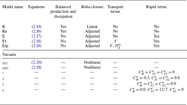

 yB
yB Rif
Rif Rif
Rif c=1.8
c=1.8 c=6.3
c=6.3 (au,av,aw)=(1.14,1.13,0.73)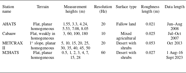

 ζ=z/Λ
ζ=z/Λ Rif
Rif yB
yB Φm
Φm −ζ<0.04
 −ζ=[0.12,1.2]
 −ζ>2
−ζ>2
 Rif
Rif Πwwtr
Πwwtr Rif
Rif
 u′2¯/e
 v′2¯/e
 w′2¯/e
 Rif
Rif Rif
Rif c=1.8
c=1.8 cu=5.42,cv=5.99,cw=−18.65
 [au,av,aw]=[1.15,1.6,0.25]
 cu=5.25,cv=7.88,cw=6.94
 [au,av,aw]=[1.22,1.12,0.66]
 u′2¯/e
 v′2¯/e
 w′2¯/e
 Rif
Rif −Rif=1
 ε
ε
 Rif
Rif TLC
TLC SSG
SSG 1
1 2
2 CBu=0.3
 CS1u=CS2u=0.6
 3
3 CBu=0.6,CS1u=CS2u=0.6
 4
4 CBu=0.6,CS1u=12/7,CS2u=0
 u′2¯/e
 v′2¯/e
 w′2¯/e
 zi/Λ
zi/Λ zi
zi Λ
Λ zi/Λ
zi/Λ −zi/Λ=3
 −zi/Λ=20
 z/Λ
z/Λ z=
z= z=
z= −ζ=[0,0.04]
 −ζ=[0.12,1.2]
 −ζ>2
−ζ>2
 λw/z
λw/z λu/Ls
λu/Ls w′3¯/w′2¯3/2
 βu
βu βuneu
βuneu βv
βv βvneu
βvneu τϵu∗l/κz
 z/Λ
z/Λ −ζ=[0,0.04]
 −ζ=[0.12,1.2]
 −ζ>2
−ζ>2
 kz
kz −ζ<0.04
 −ζ=[0.12,1.2]
 −ζ>2
−ζ>2 k=2πf/U¯
 zi/Λ
zi/Λ k−5/3
k−5/3 k−1
k−1 kz=1
kz=1 zsonic
 w′
w′ Rif
Rif
 u′2¯/e
 v′2¯/e
 w′2¯/e
 Rif
Rif kz<1/2
 kz>1
kz>1 c=1.8
c=1.8
 σdir
σdir Smv/ε
Smv/ε Co/ε
Co/ε Rif
Rif
 Rif
Rif (1/2)(εu+εv)
 εu
εu (1/2)(εucorr+εvcorr)
 εucorr
 corr
corr
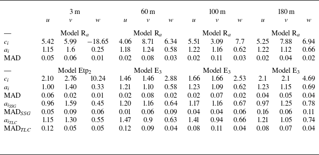
 ci
ci ai
ai a
a 2
2 CBu=0.3,CS1u=CS2u=0.6
 3
3 CBu=CS1u=CS2u=0.6


 Open access

