


1. Introduction
When there is slip in the streamwise direction at the wall, the boundary condition becomes
 \begin{equation} u-L_s\frac {\partial u}{\partial z}=0, \end{equation}
where $u$
is the streamwise velocity,
$u$
is the streamwise velocity, $L_s$
is the slip length, and
$L_s$
is the slip length, and $z$
is the wall-normal direction. The effect of wall slip on turbulent drag has been studied extensively. Min & Kim (Reference Min and Kim2004) performed direct numerical simulations (DNS) of fully developed turbulent channel flow at
$z$
is the wall-normal direction. The effect of wall slip on turbulent drag has been studied extensively. Min & Kim (Reference Min and Kim2004) performed direct numerical simulations (DNS) of fully developed turbulent channel flow at $\textit{Re}_{\tau }=180$
with Navier-slip boundary conditions. With streamwise slip only, they reported substantial drag reduction that increased with slip length, reaching approximately
$\textit{Re}_{\tau }=180$
with Navier-slip boundary conditions. With streamwise slip only, they reported substantial drag reduction that increased with slip length, reaching approximately $29\,\%$
at
$29\,\%$
at $L_s^+=3.566$
; with spanwise slip only, they observed drag increase accompanied by strengthened near-wall activity. Consistent with this, Busse & Sandham (Reference Busse and Sandham2012) showed that anisotropic slip can substantially alter drag: streamwise slip promotes drag reduction, whereas spanwise slip tends to increase drag, and they identified a threshold streamwise slip length beyond which drag is reduced irrespective of the spanwise slip. Park, Park & Kim (Reference Park, Park and Kim2013) emphasised that drag reduction correlates strongly with an effective slip length: the normalised drag decreases rapidly as the effective slip increases up to
$L_s^+=3.566$
; with spanwise slip only, they observed drag increase accompanied by strengthened near-wall activity. Consistent with this, Busse & Sandham (Reference Busse and Sandham2012) showed that anisotropic slip can substantially alter drag: streamwise slip promotes drag reduction, whereas spanwise slip tends to increase drag, and they identified a threshold streamwise slip length beyond which drag is reduced irrespective of the spanwise slip. Park, Park & Kim (Reference Park, Park and Kim2013) emphasised that drag reduction correlates strongly with an effective slip length: the normalised drag decreases rapidly as the effective slip increases up to $\lambda ^+\approx 30$
–
$\lambda ^+\approx 30$
– $40$
, after which it varies only weakly with further increases in slip. Yoon et al. (Reference Yoon, Hwang, Lee, Sung and Kim2016) reported that slip conditions elongate near-wall coherent structures, and at bulk Reynolds number
$40$
, after which it varies only weakly with further increases in slip. Yoon et al. (Reference Yoon, Hwang, Lee, Sung and Kim2016) reported that slip conditions elongate near-wall coherent structures, and at bulk Reynolds number $10{\,}333$
, yielded approximately a
$10{\,}333$
, yielded approximately a $35\,\%$
reduction in skin friction; they further estimated that large-scale structures and their near-wall imprints contribute a substantial fraction of this reduction. Finally, Ibrahim et al. (Reference Ibrahim, Gómez-de-Segura, Chung and García-Mayoral2021) proposed a unifying virtual-origin framework for turbulence over drag-altering surfaces under Robin-type constant-slip boundary conditions. A key element is the distinction between the apparent origin perceived by the mean flow,
$35\,\%$
reduction in skin friction; they further estimated that large-scale structures and their near-wall imprints contribute a substantial fraction of this reduction. Finally, Ibrahim et al. (Reference Ibrahim, Gómez-de-Segura, Chung and García-Mayoral2021) proposed a unifying virtual-origin framework for turbulence over drag-altering surfaces under Robin-type constant-slip boundary conditions. A key element is the distinction between the apparent origin perceived by the mean flow, $\ell _U$
, and that perceived by the turbulence,
$\ell _U$
, and that perceived by the turbulence, $\ell _T$
. By imposing slip in Fourier space, they showed that the streamwise slip applied to the mean mode (
$\ell _T$
. By imposing slip in Fourier space, they showed that the streamwise slip applied to the mean mode ( $k=0$
) and to the fluctuating modes (
$k=0$
) and to the fluctuating modes ( $k\neq 0$
) can be prescribed independently (i.e.
$k\neq 0$
) can be prescribed independently (i.e. $\ell _{x,m}$
versus
$\ell _{x,m}$
versus $\ell _{x,f}$
), enabling separate control of the mean flow shift and near-wall streamwise intensity within a time-invariant constant-slip setting. They also showed that
$\ell _{x,f}$
), enabling separate control of the mean flow shift and near-wall streamwise intensity within a time-invariant constant-slip setting. They also showed that $\ell _T$
is governed primarily by the cross-flow wall conditions (wall-normal and spanwise components), and that aligning the virtual origins leads to the collapse of turbulence statistics towards smooth-wall-like behaviour in appropriately shifted/scaled coordinates.
$\ell _T$
is governed primarily by the cross-flow wall conditions (wall-normal and spanwise components), and that aligning the virtual origins leads to the collapse of turbulence statistics towards smooth-wall-like behaviour in appropriately shifted/scaled coordinates.
Previous computational studies, including the ones cited above, have often modelled hydrodynamic slip as a constant parameter in the slip boundary condition. This is an oversimplification, as hydrodynamic slip is an interfacial phenomenon governed by complex interactions at the solid–liquid interface and the local wall shear stress (Thompson & Troian Reference Thompson and Troian1997; Martini et al. Reference Martini, Hsu, Patankar and Lichter2008a
; Kannam et al. Reference Kannam, Todd, Hansen and Daivis2011; Ramos-Alvarado, Kumar & Peterson Reference Ramos-Alvarado, Kumar and Peterson2016; Wagemann et al. Reference Wagemann, Oyarzua, Walther and Zambrano2017; Shuvo et al. Reference Shuvo, Paniagua-Guerra, Choi, Kim and Alvarado2025). Experimental investigations provide evidence that $L_s$
is shear-dependent. Craig, Neto & Williams (Reference Craig, Neto and Williams2001) measured hydrodynamic drainage forces in a Newtonian fluid using an atomic force microscope. Their results showed that
$L_s$
is shear-dependent. Craig, Neto & Williams (Reference Craig, Neto and Williams2001) measured hydrodynamic drainage forces in a Newtonian fluid using an atomic force microscope. Their results showed that $L_s$
increased linearly with shear rate. Choi, Westin & Breuer (Reference Choi, Westin and Breuer2003) conducted experiments on water flow in microchannels, and observed a comparable linear relationship between
$L_s$
increased linearly with shear rate. Choi, Westin & Breuer (Reference Choi, Westin and Breuer2003) conducted experiments on water flow in microchannels, and observed a comparable linear relationship between $L_s$
and shear rate. Further investigations by Li, Mo & Li (Reference Li, Mo and Li2014) revealed that
$L_s$
and shear rate. Further investigations by Li, Mo & Li (Reference Li, Mo and Li2014) revealed that $L_s$
increases linearly with shear rate once a critical shear rate is exceeded. At high shear rates,
$L_s$
increases linearly with shear rate once a critical shear rate is exceeded. At high shear rates, $L_s$
asymptotes to a constant value. This transition highlights the dual influence of solid–liquid affinity and shear rate on the development of hydrodynamic slip. While experimental techniques have advanced significantly, their resolution remains limited in capturing the full complexity of interfacial interactions. Consequently, molecular dynamics (MD) simulations have been increasingly employed to investigate atomic-scale mechanisms governing hydrodynamic slip. The behaviour of
$L_s$
asymptotes to a constant value. This transition highlights the dual influence of solid–liquid affinity and shear rate on the development of hydrodynamic slip. While experimental techniques have advanced significantly, their resolution remains limited in capturing the full complexity of interfacial interactions. Consequently, molecular dynamics (MD) simulations have been increasingly employed to investigate atomic-scale mechanisms governing hydrodynamic slip. The behaviour of $L_s$
varies significantly under different shear conditions, with reports of both bounded and unbounded growth at high shear rates. Thompson & Troian (Reference Thompson and Troian1997) performed non-equilibrium MD (NEMD) simulations of shear-driven flow, and observed that
$L_s$
varies significantly under different shear conditions, with reports of both bounded and unbounded growth at high shear rates. Thompson & Troian (Reference Thompson and Troian1997) performed non-equilibrium MD (NEMD) simulations of shear-driven flow, and observed that $L_s$
remained constant at low shear rates but exhibited rapid growth beyond a critical shear rate. Similar trends were reported in shear-driven MD simulations by Voronov, Papavassiliou & Lee (Reference Voronov, Papavassiliou and Lee2006, Reference Voronov, Papavassiliou and Lee2007) and Chen et al. (Reference Chen, Li, Jiang, Yang, Wang and Wang2006), where
$L_s$
remained constant at low shear rates but exhibited rapid growth beyond a critical shear rate. Similar trends were reported in shear-driven MD simulations by Voronov, Papavassiliou & Lee (Reference Voronov, Papavassiliou and Lee2006, Reference Voronov, Papavassiliou and Lee2007) and Chen et al. (Reference Chen, Li, Jiang, Yang, Wang and Wang2006), where $L_s$
increased sharply after exceeding a critical shear threshold. Conversely, Martini et al. (Reference Martini, Hsu, Patankar and Lichter2008a
) argued that the unbounded growth of
$L_s$
increased sharply after exceeding a critical shear threshold. Conversely, Martini et al. (Reference Martini, Hsu, Patankar and Lichter2008a
) argued that the unbounded growth of $L_s$
at high shear rates was an artefact of rigid wall models that neglect solid–liquid momentum exchange. Using NEMD simulations of Couette flow, they showed that while rigid walls yield unbounded
$L_s$
at high shear rates was an artefact of rigid wall models that neglect solid–liquid momentum exchange. Using NEMD simulations of Couette flow, they showed that while rigid walls yield unbounded $L_s$
, flexible walls accounting for atomic vibrations and viscous dissipation produce bounded
$L_s$
, flexible walls accounting for atomic vibrations and viscous dissipation produce bounded $L_s$
. Furthermore, other studies have reported a reduction in
$L_s$
. Furthermore, other studies have reported a reduction in $L_s$
at high shear rates (Alizadeh Pahlavan & Freund Reference Alizadeh Pahlavan and Freund2011; Ramos-Alvarado et al. Reference Ramos-Alvarado, Kumar and Peterson2016). Alizadeh Pahlavan & Freund (Reference Alizadeh Pahlavan and Freund2011) attributed this reduction to local viscous heating caused by an increase in solid–liquid collisions. These contrasting findings suggest that the dependence of
$L_s$
at high shear rates (Alizadeh Pahlavan & Freund Reference Alizadeh Pahlavan and Freund2011; Ramos-Alvarado et al. Reference Ramos-Alvarado, Kumar and Peterson2016). Alizadeh Pahlavan & Freund (Reference Alizadeh Pahlavan and Freund2011) attributed this reduction to local viscous heating caused by an increase in solid–liquid collisions. These contrasting findings suggest that the dependence of $L_s$
on shear rate and interfacial properties remains unclear.
$L_s$
on shear rate and interfacial properties remains unclear.
Despite extensive molecular-scale insights, few continuum-scale models have incorporated shear-dependent slip boundary conditions derived from MD simulations. In the present work, we performed NEMD simulations of shear-driven flow to characterise the behaviour of $L_s$
under different solid–liquid interactions, ranging from hydrophilic to hydrophobic conditions. Based on these findings, we formulated a shear- and interaction-dependent
$L_s$
under different solid–liquid interactions, ranging from hydrophilic to hydrophobic conditions. Based on these findings, we formulated a shear- and interaction-dependent $L_s$
model, and incorporated it into DNS of turbulent channel flows. The DNS framework enables us to investigate the impact of this molecular-level-informed slip boundary condition on near-wall turbulence structures and statistics. In addition, we developed a model for the mean momentum balance incorporating shear-dependent
$L_s$
model, and incorporated it into DNS of turbulent channel flows. The DNS framework enables us to investigate the impact of this molecular-level-informed slip boundary condition on near-wall turbulence structures and statistics. In addition, we developed a model for the mean momentum balance incorporating shear-dependent $L_s$
, aiming to predict velocity profiles and near-wall turbulence intensity. This multiscale approach offers a physically grounded framework that links molecular interfacial behaviour with continuum turbulence modelling, enabling a deeper understanding of slip effects in wall-bounded turbulent flows.
$L_s$
, aiming to predict velocity profiles and near-wall turbulence intensity. This multiscale approach offers a physically grounded framework that links molecular interfacial behaviour with continuum turbulence modelling, enabling a deeper understanding of slip effects in wall-bounded turbulent flows.
2. Computational details
2.1. The MD simulation set-up
The MD simulations provide a molecular-level framework capable of resolving interfacial phenomena beyond the continuum approximation of the Navier–Stokes equations (Thompson & Troian Reference Thompson and Troian1997; Martini et al. Reference Martini, Hsu, Patankar and Lichter2008a
; Alizadeh Pahlavan & Freund Reference Alizadeh Pahlavan and Freund2011; Ramos-Alvarado et al. Reference Ramos-Alvarado, Kumar and Peterson2016; Shuvo et al. Reference Shuvo, Gonzalez-Valle, Yang and Ramos-Alvarado2024a
, Reference Shuvo, Paniagua-Guerra, Choi, Kim and Alvarado2025). They solve Newton’s second law of motion ( $F=ma$
), where
$F=ma$
), where $F$
represents the force acting on an atom,
$F$
represents the force acting on an atom, $m$
is the atomic mass, and
$m$
is the atomic mass, and $a$
is its acceleration. In MD simulations,
$a$
is its acceleration. In MD simulations, $F$
is calculated using an empirical force field, which defines the potential energy landscape as a function of the relative distance between atoms (Rapaport Reference Rapaport2004; Frenkel & Smit Reference Frenkel and Smit2023). This classical framework captures the essential physics of bonded and non-bonded interactions, thereby facilitating the calculation of
$F$
is calculated using an empirical force field, which defines the potential energy landscape as a function of the relative distance between atoms (Rapaport Reference Rapaport2004; Frenkel & Smit Reference Frenkel and Smit2023). This classical framework captures the essential physics of bonded and non-bonded interactions, thereby facilitating the calculation of $L_s$
as a function of interfacial properties and operating conditions.
$L_s$
as a function of interfacial properties and operating conditions.
(a) Computational domain of an MD shear-driven flow model. (b) Computational domain for DNS with shear-dependent $L_s$
.
$L_s$
.

In our MD simulations, we investigated shear-driven water flow confined between two parallel graphite walls to elucidate the influence of solid–liquid affinity on $L_s$
; see figure 1(a). The MD simulations were conducted using the large-scale atomic/molecular massively parallel simulator (LAMMPS) (Plimpton Reference Plimpton1995), and the atomic trajectories were visualised using OVITO (Stukowski Reference Stukowski2009). To model shear-driven flow, we confined water molecules between two atomistically smooth graphite slabs. The simulation box was periodic in the
$L_s$
; see figure 1(a). The MD simulations were conducted using the large-scale atomic/molecular massively parallel simulator (LAMMPS) (Plimpton Reference Plimpton1995), and the atomic trajectories were visualised using OVITO (Stukowski Reference Stukowski2009). To model shear-driven flow, we confined water molecules between two atomistically smooth graphite slabs. The simulation box was periodic in the $x$
- and
$x$
- and $y$
-directions, while the
$y$
-directions, while the $z$
-direction, normal to the flow, was fixed and non-periodic. In this fixed boundary condition, atoms were not allowed to move across or interact with the opposite side of the simulation box along the z-direction. The outermost graphene layers were excluded from time integration to maintain a constant channel height throughout the simulation.
$z$
-direction, normal to the flow, was fixed and non-periodic. In this fixed boundary condition, atoms were not allowed to move across or interact with the opposite side of the simulation box along the z-direction. The outermost graphene layers were excluded from time integration to maintain a constant channel height throughout the simulation.
The carbon atoms in the graphene sheets were modelled with a Tersoff (Lindsay & Broido Reference Lindsay and Broido2010) force field, and the weak non-bonded graphene interlayer interactions were modelled with a Lennard-Jones (LJ) (Lindsay, Broido & Mingo Reference Lindsay, Broido and Mingo2011) force field. The LJ force field, commonly used to model non-bonded interactions, is expressed as
 \begin{equation} V(r) = 4\epsilon \left (\frac {\sigma ^{12}}{r^{12}}-\frac {\sigma ^{6}}{r^{6}}\right ), \end{equation}
where $V$
is the pairwise interaction energy as a function of the interatomic separation
$V$
is the pairwise interaction energy as a function of the interatomic separation $r$
,
$r$
, $\epsilon$
defines the depth of the potential well (energy scale), and
$\epsilon$
defines the depth of the potential well (energy scale), and $\sigma$
represents the finite distance at which the potential energy becomes zero (length scale). In our simulations, graphite was selected as the wall material due to its broadly characterised interactions with water. The simulation domain consisted of graphite slabs measuring 62
$\sigma$
represents the finite distance at which the potential energy becomes zero (length scale). In our simulations, graphite was selected as the wall material due to its broadly characterised interactions with water. The simulation domain consisted of graphite slabs measuring 62 $\unicode{x00C5}$ $\times$
54
$\times$
54 $\unicode{x00C5}$
in the
$\unicode{x00C5}$
in the $x{-}y$
plane, with thickness
$x{-}y$
plane, with thickness $20\ \unicode{x00C5}$
. A total of 5491 water molecules occupied the gap between these solid surfaces, and the extended simple point charge model (SPC/E) in Ryckaert, Ciccotti & Berendsen (Reference Ryckaert, Ciccotti and Berendsen1977) and Ciccotti & Ryckaert (Reference Ciccotti and Ryckaert1986) was used to model its molecular interactions. The initial separation between the confining surfaces was approximately 50
$20\ \unicode{x00C5}$
. A total of 5491 water molecules occupied the gap between these solid surfaces, and the extended simple point charge model (SPC/E) in Ryckaert, Ciccotti & Berendsen (Reference Ryckaert, Ciccotti and Berendsen1977) and Ciccotti & Ryckaert (Reference Ciccotti and Ryckaert1986) was used to model its molecular interactions. The initial separation between the confining surfaces was approximately 50 $\unicode{x00C5}$
. This distance was slightly adjusted to ensure that the bulk region of water, located sufficiently far from the solid–liquid interfaces, attained density
$\unicode{x00C5}$
. This distance was slightly adjusted to ensure that the bulk region of water, located sufficiently far from the solid–liquid interfaces, attained density $1.00\ \pm \ 0.02$ $\textrm{g cm}^{-3}$
at 300 K. Upon reaching the target density, the system was deemed to have achieved a compressibility-free state at the corresponding temperature and density; see figure 2(a). Three distinct solid–liquid interactions were studied, corresponding to varying degrees of surface wettability and interfacial affinity. The interfacial interactions were modelled using the LJ potential. Traditionally, cross-interaction parameters in LJ models are determined using the Lorentz–Berthelot mixing rules (Lorentz Reference Lorentz1881), where the energy scale is defined as the geometric mean
$\textrm{g cm}^{-3}$
at 300 K. Upon reaching the target density, the system was deemed to have achieved a compressibility-free state at the corresponding temperature and density; see figure 2(a). Three distinct solid–liquid interactions were studied, corresponding to varying degrees of surface wettability and interfacial affinity. The interfacial interactions were modelled using the LJ potential. Traditionally, cross-interaction parameters in LJ models are determined using the Lorentz–Berthelot mixing rules (Lorentz Reference Lorentz1881), where the energy scale is defined as the geometric mean $\epsilon _{\textit{ij}}=(\epsilon _{\textit{ii}}\epsilon _{\textit{jj}})^{1/2}$
, and the length scale as the arithmetic mean
$\epsilon _{\textit{ij}}=(\epsilon _{\textit{ii}}\epsilon _{\textit{jj}})^{1/2}$
, and the length scale as the arithmetic mean $\sigma _{\textit{ij}}=(\sigma _{\textit{ii}}+\sigma _{\textit{jj}})/2$
, of the LJ parameters optimised for the individual interface components. Although widespread in the literature, this practice has been deemed inadequate (Thompson & Troian Reference Thompson and Troian1997; Voronov et al. Reference Voronov, Papavassiliou and Lee2006, Reference Voronov, Papavassiliou and Lee2007; Petravic & Harrowell Reference Petravic and Harrowell2007). Alternatively, the solid–liquid LJ parameters can be optimised by fitting adsorption energy profiles obtained from first principles data such as Møller–Plesset perturbation theory of the second order (MP2) (Wu & Aluru Reference Wu and Aluru2013), density functional theory with symmetry-adapted perturbation theory (DFT–SAPT) (Jenness, Karalti & Jordan Reference Jenness, Karalti and Jordan2010), the random phase approximation (Ma et al. Reference Ma, Michaelides, Alfe, Schimka, Kresse and Wang2011), or coupled-cluster calculations with single and double excitations and perturbative triples (CCSD(T)) (Voloshina et al. Reference Voloshina, Usvyat, Schütz, Dedkov and Paulus2011). In this study, three distinct solid–liquid interfaces were considered, corresponding to strong, moderate and weak interaction strengths. The LJ parameters for the strong interaction case were optimised by Wu & Aluru (Reference Wu and Aluru2013) using CCSD(T)-based adsorption energy data, where both C–O and C–H interactions were parametrised by fitting to a single adsorption curve. The parameters for the moderate interaction case were adopted from Ramos-Alvarado (Reference Ramos-Alvarado2019), who optimised C–O and C–H LJ parameters by fitting two adsorption curves obtained from random phase approximation data reported by Ma et al. (Reference Ma, Michaelides, Alfe, Schimka, Kresse and Wang2011). Furthermore, the LJ parameters for the weak interaction case (C–O only) were obtained from Paniagua-Guerra et al. (Reference Paniagua-Guerra, Gonzalez-Valle and Ramos-Alvarado2020), who employed the wettability–binding energy relationship proposed by Ramos-Alvarado (Reference Ramos-Alvarado2019). This relationship provides an analytical connection between the LJ parameters and the equilibrium contact angle, verified through MD simulations, where the LJ parameters serve as input, and a size-independent contact angle emerges as the output. The corresponding LJ parameters for the three interface models are summarised in table 1. The resulting interfaces exhibited contact angles ranging from fully wetting (
$\sigma _{\textit{ij}}=(\sigma _{\textit{ii}}+\sigma _{\textit{jj}})/2$
, of the LJ parameters optimised for the individual interface components. Although widespread in the literature, this practice has been deemed inadequate (Thompson & Troian Reference Thompson and Troian1997; Voronov et al. Reference Voronov, Papavassiliou and Lee2006, Reference Voronov, Papavassiliou and Lee2007; Petravic & Harrowell Reference Petravic and Harrowell2007). Alternatively, the solid–liquid LJ parameters can be optimised by fitting adsorption energy profiles obtained from first principles data such as Møller–Plesset perturbation theory of the second order (MP2) (Wu & Aluru Reference Wu and Aluru2013), density functional theory with symmetry-adapted perturbation theory (DFT–SAPT) (Jenness, Karalti & Jordan Reference Jenness, Karalti and Jordan2010), the random phase approximation (Ma et al. Reference Ma, Michaelides, Alfe, Schimka, Kresse and Wang2011), or coupled-cluster calculations with single and double excitations and perturbative triples (CCSD(T)) (Voloshina et al. Reference Voloshina, Usvyat, Schütz, Dedkov and Paulus2011). In this study, three distinct solid–liquid interfaces were considered, corresponding to strong, moderate and weak interaction strengths. The LJ parameters for the strong interaction case were optimised by Wu & Aluru (Reference Wu and Aluru2013) using CCSD(T)-based adsorption energy data, where both C–O and C–H interactions were parametrised by fitting to a single adsorption curve. The parameters for the moderate interaction case were adopted from Ramos-Alvarado (Reference Ramos-Alvarado2019), who optimised C–O and C–H LJ parameters by fitting two adsorption curves obtained from random phase approximation data reported by Ma et al. (Reference Ma, Michaelides, Alfe, Schimka, Kresse and Wang2011). Furthermore, the LJ parameters for the weak interaction case (C–O only) were obtained from Paniagua-Guerra et al. (Reference Paniagua-Guerra, Gonzalez-Valle and Ramos-Alvarado2020), who employed the wettability–binding energy relationship proposed by Ramos-Alvarado (Reference Ramos-Alvarado2019). This relationship provides an analytical connection between the LJ parameters and the equilibrium contact angle, verified through MD simulations, where the LJ parameters serve as input, and a size-independent contact angle emerges as the output. The corresponding LJ parameters for the three interface models are summarised in table 1. The resulting interfaces exhibited contact angles ranging from fully wetting ( $0^\circ$
) to partially hydrophilic (
$0^\circ$
) to partially hydrophilic ( $64.4^\circ$
).
$64.4^\circ$
).
(a) Water density profiles for the difference interfacial models. (b) Schematic of the velocity profile in Couette flow. The shear rate is calculated from the slope of the velocity profile ${\textrm{d}}u/{\textrm{d}}z$
.
${\textrm{d}}u/{\textrm{d}}z$
.

In MD shear-driven flow, we applied shear by translating the top wall with a constant velocity ranging from 0.8 to 6 $\unicode{x00C5}$
ps
$\unicode{x00C5}$
ps $^{-1}$
, while keeping the bottom wall stationary. This approach for shear-driven flow in MD was adopted in previous literature (Thompson & Troian Reference Thompson and Troian1997; Voronov et al. Reference Voronov, Papavassiliou and Lee2006, Reference Voronov, Papavassiliou and Lee2007; Ho et al. Reference Ho, Papavassiliou, Lee and Striolo2011). The resulting shear rate in our simulation for each interfacial model was determined from the slope of the steady-state velocity profile, as illustrated in figure 2(b). Accordingly, the shear rate (
$^{-1}$
, while keeping the bottom wall stationary. This approach for shear-driven flow in MD was adopted in previous literature (Thompson & Troian Reference Thompson and Troian1997; Voronov et al. Reference Voronov, Papavassiliou and Lee2006, Reference Voronov, Papavassiliou and Lee2007; Ho et al. Reference Ho, Papavassiliou, Lee and Striolo2011). The resulting shear rate in our simulation for each interfacial model was determined from the slope of the steady-state velocity profile, as illustrated in figure 2(b). Accordingly, the shear rate ( $\dot \gamma _f$
) in the NEMD simulations varied between
$\dot \gamma _f$
) in the NEMD simulations varied between $0.001$
and
$0.001$
and $0.04$
ps
$0.04$
ps $^{-1}$
.
$^{-1}$
.
The LJ parameters used for the interface models. The weak interaction includes only C–O interactions, while the moderate and strong interactions incorporate both C–O and C–H interactions.

Previous studies (Kannam et al. Reference Kannam, Todd, Hansen and Daivis2011, Reference Kannam, Todd, Hansen and Daivis2012; Ramos-Alvarado et al. Reference Ramos-Alvarado, Kumar and Peterson2016) have also reported that in the low-shear regime, $L_s$
values obtained from NEMD simulations are consistent with those computed using equilibrium molecular dynamic (EMD), where the interfacial friction coefficient is evaluated through Green–Kubo relations derived from fluctuation–dissipation theory. In our simulations, we observe a similar level of consistency: the slip lengths obtained at low shear rates agree closely with the EMD results reported by Paniagua-Guerra et al. (Reference Paniagua-Guerra, Gonzalez-Valle and Ramos-Alvarado2020), as shown in supplementary figure S1.
$L_s$
values obtained from NEMD simulations are consistent with those computed using equilibrium molecular dynamic (EMD), where the interfacial friction coefficient is evaluated through Green–Kubo relations derived from fluctuation–dissipation theory. In our simulations, we observe a similar level of consistency: the slip lengths obtained at low shear rates agree closely with the EMD results reported by Paniagua-Guerra et al. (Reference Paniagua-Guerra, Gonzalez-Valle and Ramos-Alvarado2020), as shown in supplementary figure S1.
As MD simulations of flow require relatively high shear rates to produce noise-free data to bypass the short length scale and time scale compared to experimental conditions, the elevated shear rates induce significant viscous heating within the fluid, necessitating a means of thermal regulation. Several thermostating strategies exist, including applying a thermostat to all atoms (Thompson & Robbins Reference Thompson and Robbins1990; Khare, Keblinski & Yethiraj Reference Khare, Keblinski and Yethiraj2006; Voronov et al. Reference Voronov, Papavassiliou and Lee2006), only to fluid atoms (Voronov et al. Reference Voronov, Papavassiliou and Lee2007; Thomas & McGaughey Reference Thomas and McGaughey2008; Zhang, Zhang & Ye Reference Zhang, Zhang and Ye2009), or only to solid atoms (Nagayama & Cheng Reference Nagayama and Cheng2004; Martini et al. Reference Martini, Hsu, Patankar and Lichter2008a ; Hansen, Todd & Daivis Reference Hansen, Todd and Daivis2011; Kannam et al. Reference Kannam, Todd, Hansen and Daivis2011, Reference Kannam, Todd, Hansen and Daivis2012; Yong & Zhang Reference Yong and Zhang2013). Thermostating of the fluid atoms interrupts the natural flow dynamics by rescaling the velocity of the fluid particles, resulting in unphysical flow conditions (see Yong & Zhang Reference Yong and Zhang2013). In contrast, thermostating the solid wall provides a more physically consistent approach by mimicking heat transfer through a conductive boundary. In our simulations, a Nosè–Hoover (Hoover Reference Hoover1985) thermostat with time constant 0.1 ps was applied to the bottom graphite wall and maintained at 300 K to dissipate the excess heat generated by shear. The top wall was adiabatic, ensuring that heat was removed solely through the bottom surface, mimicking natural cooling.
The MD simulations were carried out in two stages: EMD and NEMD. In the EMD stage, the system was first equilibrated at 300 K for 1000 ps using the canonical ensemble (NVT), followed by an additional 1000 ps under the microcanonical ensemble (NVE) to verify the system’s stability without external thermal control. In the NEMD stage, shear was applied by translating the top wall at a constant velocity. Each simulation was first run for 2000 ps to reach a statistically steady state, followed by a 5000 ps production run for data collection, with sampling performed every 0.5 ps. During NEMD simulations, the water molecules were integrated using pure Newtonian dynamics (no thermostat). The time step for the simulations was 0.001 ps.
2.2. The DNS set-up
The computational domain for DNS is a half-channel configuration, as illustrated in figure 1(b). The coordinate system is defined with $x$
,
$x$
, $y$
and
$y$
and $z$
representing the streamwise, spanwise and wall-normal directions, respectively. Periodic boundary conditions are applied in the streamwise and spanwise directions. A stress-free boundary condition, defined as
$z$
representing the streamwise, spanwise and wall-normal directions, respectively. Periodic boundary conditions are applied in the streamwise and spanwise directions. A stress-free boundary condition, defined as ${\partial u}/{\partial z}={\partial v}/{\partial z}=0$
and
${\partial u}/{\partial z}={\partial v}/{\partial z}=0$
and $w=0$
, was applied at the top boundary, while an MD-informed shear-dependent slip condition was used at the bottom wall. In our DNS framework, a constant streamwise pressure gradient
$w=0$
, was applied at the top boundary, while an MD-informed shear-dependent slip condition was used at the bottom wall. In our DNS framework, a constant streamwise pressure gradient ${\textrm{d}}p/{\textrm{d}}x=1$
was applied. The mean wall shear stress was therefore
${\textrm{d}}p/{\textrm{d}}x=1$
was applied. The mean wall shear stress was therefore $\tau _m=1$
due to force balance. Accordingly, the friction velocity was 1 in all DNS. A detailed formulation and discussion of the shear-dependent slip condition is presented in § 4.
$\tau _m=1$
due to force balance. Accordingly, the friction velocity was 1 in all DNS. A detailed formulation and discussion of the shear-dependent slip condition is presented in § 4.
The computational domain spans $L_x = 8\pi \delta$
in the streamwise direction and
$L_x = 8\pi \delta$
in the streamwise direction and $L_y = 3\pi \delta$
in the spanwise direction (where
$L_y = 3\pi \delta$
in the spanwise direction (where $\delta =1$
is the channel half-height); the wall-normal extent is
$\delta =1$
is the channel half-height); the wall-normal extent is $\delta$
. Uniform grid spacing is employed in the homogeneous directions, with
$\delta$
. Uniform grid spacing is employed in the homogeneous directions, with $\Delta x^+ \approx 12$
and
$\Delta x^+ \approx 12$
and $\Delta y^+ \approx 6$
. The solver is pseudo-spectral in the streamwise and spanwise directions, for which grids slightly coarser than the conventional
$\Delta y^+ \approx 6$
. The solver is pseudo-spectral in the streamwise and spanwise directions, for which grids slightly coarser than the conventional $\Delta x^+ \approx 10$
and
$\Delta x^+ \approx 10$
and $\Delta y^+ \approx 5$
are generally adequate (Bernardini, Pirozzoli & Orlandi Reference Bernardini, Pirozzoli and Orlandi2014; Oliver et al. Reference Oliver, Malaya, Ulerich and Moser2014; Thompson et al. Reference Thompson, Sampaio, de Bragança, Felipe, Thais and Mompean2016; Chen et al. Reference Chen, Lv, Xu, Shi and Yang2022).
$\Delta y^+ \approx 5$
are generally adequate (Bernardini, Pirozzoli & Orlandi Reference Bernardini, Pirozzoli and Orlandi2014; Oliver et al. Reference Oliver, Malaya, Ulerich and Moser2014; Thompson et al. Reference Thompson, Sampaio, de Bragança, Felipe, Thais and Mompean2016; Chen et al. Reference Chen, Lv, Xu, Shi and Yang2022).
The wall-normal resolution is determined following the recommendations of Yang & Griffin (Reference Yang and Griffin2021) and Pirozzoli & Orlandi (Reference Pirozzoli and Orlandi2021). Accordingly, a non-uniform mesh is adopted to resolve the wall unit in the viscous sublayer, and the local Kolmogorov length scale in the logarithmic and outer regions. The minimum and maximum wall-normal spacings are $\Delta z_{\textit{min}}^+ \approx 0.34$
and
$\Delta z_{\textit{min}}^+ \approx 0.34$
and $\Delta z_{\textit{max}}^+ \approx 3.73$
for
$\Delta z_{\textit{max}}^+ \approx 3.73$
for $\textit{Re}_{\tau } = 180$
,
$\textit{Re}_{\tau } = 180$
, $\Delta z_{\textit{min}}^+ \approx 0.47$
and
$\Delta z_{\textit{min}}^+ \approx 0.47$
and $\Delta z_{\textit{max}}^+ \approx 5.17$
for
$\Delta z_{\textit{max}}^+ \approx 5.17$
for $\textit{Re}_{\tau } = 400$
, and
$\textit{Re}_{\tau } = 400$
, and $\Delta z_{\textit{min}}^+ \approx 0.59$
and
$\Delta z_{\textit{min}}^+ \approx 0.59$
and $\Delta z_{\textit{max}}^+ \approx 6.47$
for
$\Delta z_{\textit{max}}^+ \approx 6.47$
for $\textit{Re}_{\tau } = 1000$
, ensuring adequate near-wall resolution without over-resolving the channel core. The sampling duration in each case satisfies the heuristic requirement of approximately
$\textit{Re}_{\tau } = 1000$
, ensuring adequate near-wall resolution without over-resolving the channel core. The sampling duration in each case satisfies the heuristic requirement of approximately $10\delta /u_\tau$
(Pirozzoli, Bernardini & Orlandi Reference Pirozzoli, Bernardini and Orlandi2016), ensuring statistical convergence of the first- and second-order turbulence statistics. To validate our DNS code, simulations with constant
$10\delta /u_\tau$
(Pirozzoli, Bernardini & Orlandi Reference Pirozzoli, Bernardini and Orlandi2016), ensuring statistical convergence of the first- and second-order turbulence statistics. To validate our DNS code, simulations with constant $L_s=0.02\delta$
were performed, matching the configuration of Min & Kim (Reference Min and Kim2004). Very good agreement was observed between the present results and those of Min & Kim (Reference Min and Kim2004), as shown in supplementary figure S2.
$L_s=0.02\delta$
were performed, matching the configuration of Min & Kim (Reference Min and Kim2004). Very good agreement was observed between the present results and those of Min & Kim (Reference Min and Kim2004), as shown in supplementary figure S2.
The DNS are performed using LESGO, an open-source parallel pseudo-spectral large-eddy simulation code. It solves the filtered Navier–Stokes equations using pseudo-spectral discretisation in the streamwise and spanwise directions, and a second-order finite-difference scheme in the wall-normal direction. The LESGO code, along with its modified implementations, has been extensively utilised in numerous investigations of turbulent channel flows, as evidenced by prior studies (see Bou-Zeid, Meneveau & Parlange Reference Bou-Zeid, Meneveau and Parlange2005; Anderson & Meneveau Reference Anderson and Meneveau2011; Abkar & Porté-Agel Reference Abkar and Porté-Agel2012; Zhu et al. Reference Zhu, Iungo, Leonardi and Anderson2017; Yang et al. Reference Yang, Xu, Huang and Ge2019).
The MD results, showing the slip length $L_s$
as a function of shear rate. The boundary between the two shaded regions represents the critical shear rate. The dashed lines are the sigmoid fittings. The fitted parameters are listed in table 2.
$L_s$
as a function of shear rate. The boundary between the two shaded regions represents the critical shear rate. The dashed lines are the sigmoid fittings. The fitted parameters are listed in table 2.

3. The MD results
Figure 3 illustrates the variation of $L_s$
as a function of the shear stress for different interface affinity levels. We see that in all cases,
$L_s$
as a function of the shear stress for different interface affinity levels. We see that in all cases, $L_s$
exhibits a bimodal dependence on shear, characterised by two distinct regimes: a low-shear regime (LSR) and a high-shear regime (HSR), separated by a sharp transition. Furthermore, this bimodal behaviour can be captured by a sigmoid function. Accordingly,
$L_s$
exhibits a bimodal dependence on shear, characterised by two distinct regimes: a low-shear regime (LSR) and a high-shear regime (HSR), separated by a sharp transition. Furthermore, this bimodal behaviour can be captured by a sigmoid function. Accordingly, $L_s$
values for different interface models were fitted using the sigmoid expression
$L_s$
values for different interface models were fitted using the sigmoid expression $L_s = (L_{\textit{HSR}}-L_{\textit{LSR}})/(1+\textrm{exp}[-(\dot \gamma _f-\dot \gamma _c)/\dot \gamma _t])+L_{\textit{LSR}}$
, where
$L_s = (L_{\textit{HSR}}-L_{\textit{LSR}})/(1+\textrm{exp}[-(\dot \gamma _f-\dot \gamma _c)/\dot \gamma _t])+L_{\textit{LSR}}$
, where $\dot {\gamma }_c$
and
$\dot {\gamma }_c$
and $\dot {\gamma }_t$
are fitting parameters. Here,
$\dot {\gamma }_t$
are fitting parameters. Here, $\dot {\gamma }_c$
represents the transition point from LSR to HSR, and
$\dot {\gamma }_c$
represents the transition point from LSR to HSR, and $\dot {\gamma }_t$
determines the sharpness of the transition. The MD data showed good agreement with the sigmoid fits, as indicated by the dashed lines in figure 3. The corresponding
$\dot {\gamma }_t$
determines the sharpness of the transition. The MD data showed good agreement with the sigmoid fits, as indicated by the dashed lines in figure 3. The corresponding $R^2$
values for the weak, moderate and strong interaction cases were 0.83, 0.95 and 0.79, respectively. The fitted parameters are listed in table 2. This motivates the development of a phenomenological model for the DNS study, which is discussed in § 4.
$R^2$
values for the weak, moderate and strong interaction cases were 0.83, 0.95 and 0.79, respectively. The fitted parameters are listed in table 2. This motivates the development of a phenomenological model for the DNS study, which is discussed in § 4.
Fitted parameters ( $\dot {\gamma }_c$
and
$\dot {\gamma }_c$
and $\dot {\gamma }_t$
) for the sigmoid function describing the shear-dependent slip length (
$\dot {\gamma }_t$
) for the sigmoid function describing the shear-dependent slip length ( $L_s$
) obtained from MD simulations. Here,
$L_s$
) obtained from MD simulations. Here, $\dot {\gamma }_c$
represents the critical shear rate marking the transition from the LSR to HSR, and
$\dot {\gamma }_c$
represents the critical shear rate marking the transition from the LSR to HSR, and $\dot {\gamma }_t$
characterises the sharpness of the transition.
$\dot {\gamma }_t$
characterises the sharpness of the transition.

Note that previous studies have reported contrasting trends in the shear dependence of $L_s$
. Thompson & Troian (Reference Thompson and Troian1997), Kannam et al. (Reference Kannam, Todd, Hansen and Daivis2011, Reference Kannam, Todd, Hansen and Daivis2012) and Wagemann et al. (Reference Wagemann, Oyarzua, Walther and Zambrano2017) reported an unbounded growth of
$L_s$
. Thompson & Troian (Reference Thompson and Troian1997), Kannam et al. (Reference Kannam, Todd, Hansen and Daivis2011, Reference Kannam, Todd, Hansen and Daivis2012) and Wagemann et al. (Reference Wagemann, Oyarzua, Walther and Zambrano2017) reported an unbounded growth of $L_s$
with increasing shear rates. This unbounded growth of
$L_s$
with increasing shear rates. This unbounded growth of $L_s$
with shear can be attributed to the use of rigid/fixed wall atoms in earlier studies, which suppressed momentum transfer between the wall and liquid atoms. This was verified in Martini et al. (Reference Martini, Hsu, Patankar and Lichter2008a
), who conducted simulations with both fixed- and flexible-wall atoms. Their results showed that rigid walls led to an unbounded growth of
$L_s$
with shear can be attributed to the use of rigid/fixed wall atoms in earlier studies, which suppressed momentum transfer between the wall and liquid atoms. This was verified in Martini et al. (Reference Martini, Hsu, Patankar and Lichter2008a
), who conducted simulations with both fixed- and flexible-wall atoms. Their results showed that rigid walls led to an unbounded growth of $L_s$
at high shear rates, while flexible walls produced a bounded growth of
$L_s$
at high shear rates, while flexible walls produced a bounded growth of $L_s$
.
$L_s$
.
Schematic of rigid and flexible walls in MD simulations.

Figure 4 schematically illustrates the different wall conditions used in MD simulations. In the rigid- or fixed-wall configuration, the solid atoms are excluded from time integration, ensuring that their positions remain immobile throughout the simulation (left-hand panel). This approach is computationally cheap but neglects atomic vibrations and consequently the exchange of energy and momentum between the solid and the fluid (see Martini et al. Reference Martini, Hsu, Patankar and Lichter2008a ). At finite temperatures, however, solid atoms possess non-zero kinetic energy and vibrate around their equilibrium positions (middle panel). These thermal vibrations are essential for maintaining thermodynamic consistency, as they enable realistic coupling between the wall and the fluid. To prevent unphysical centre-of-mass drift of the solid wall – while still retaining natural thermal motion – an invisible tether was applied to each solid atom (right-hand panel). This tethering technique acts as an elastic spring that anchors atoms to their equilibrium lattice positions without freezing them. The tether constrains translational motion of the solid but allows atoms to vibrate freely within the potential well defined by the spring, thereby preserving the thermal motion and realistic energy exchange characteristic of a flexible-wall model. In our shear-driven flow simulations, the bottom solid wall was tethered to prevent unwanted drift arising from the high shear rates applied to the top wall.
The bimodal behaviour of $L_s$
with respect to shear has been interpreted through several theoretical frameworks. Martini et al. (Reference Martini, Roxin, Snurr, Wang and Lichter2008b
) employed the variable-density Frenkel–Kontorova model (Lichter, Roxin & Mandre Reference Lichter, Roxin and Mandre2004). At low shear rates, they identified a defect slip, where liquid molecules transition discretely by jumping from one equilibrium site to another. As the shear rate increases, this localised hopping mechanism gives way to a global slip in which the entire liquid layer moves collectively. Similarly, Babu & Sathian (Reference Babu and Sathian2012) described shear-dependent
$L_s$
with respect to shear has been interpreted through several theoretical frameworks. Martini et al. (Reference Martini, Roxin, Snurr, Wang and Lichter2008b
) employed the variable-density Frenkel–Kontorova model (Lichter, Roxin & Mandre Reference Lichter, Roxin and Mandre2004). At low shear rates, they identified a defect slip, where liquid molecules transition discretely by jumping from one equilibrium site to another. As the shear rate increases, this localised hopping mechanism gives way to a global slip in which the entire liquid layer moves collectively. Similarly, Babu & Sathian (Reference Babu and Sathian2012) described shear-dependent $L_s$
behaviour based on transition-state theory. They suggested that liquid molecules need to overcome an activation energy barrier to jump from one equilibrium position to another. The transition from the LSR to the HSR occurs when the applied shear stress overcomes the activation energy for momentum transfer. An experimental study by Li et al. (Reference Li, Mo and Li2014) provided additional support for the LSR-to-HSR transition. In their investigation of Poiseuille flow in silicon nanochannels, they observed a sharp increase in
$L_s$
behaviour based on transition-state theory. They suggested that liquid molecules need to overcome an activation energy barrier to jump from one equilibrium position to another. The transition from the LSR to the HSR occurs when the applied shear stress overcomes the activation energy for momentum transfer. An experimental study by Li et al. (Reference Li, Mo and Li2014) provided additional support for the LSR-to-HSR transition. In their investigation of Poiseuille flow in silicon nanochannels, they observed a sharp increase in $L_s$
when the applied pressure gradient matched the adhesive forces between the liquid and the wall. Beyond this threshold, further increases in shear rate resulted in a plateau in the measured
$L_s$
when the applied pressure gradient matched the adhesive forces between the liquid and the wall. Beyond this threshold, further increases in shear rate resulted in a plateau in the measured $L_s$
. More recently, Shuvo et al. (Reference Shuvo, Paniagua-Guerra, Yang and Ramos-Alvarado2024b
) explored the rheology of water and the friction coefficient at the interface to understand the bimodal response of
$L_s$
. More recently, Shuvo et al. (Reference Shuvo, Paniagua-Guerra, Yang and Ramos-Alvarado2024b
) explored the rheology of water and the friction coefficient at the interface to understand the bimodal response of $L_s$
. They indicate that while both the viscosity and the friction coefficient remain approximately constant at low shear, they decrease at higher shear rates. Notably, the friction coefficient declined more rapidly than the viscosity during the transition, resulting in an effective increase in slip length. In the HSR, the system reached a new steady state in which
$L_s$
. They indicate that while both the viscosity and the friction coefficient remain approximately constant at low shear, they decrease at higher shear rates. Notably, the friction coefficient declined more rapidly than the viscosity during the transition, resulting in an effective increase in slip length. In the HSR, the system reached a new steady state in which $L_s$
became approximately constant.
$L_s$
became approximately constant.
Density contours of water in (a) weak interaction, (b) moderate interaction, (c) strong interaction. The white gap is the complete repulsion region.

The LSR-to-HSR transition observed in our MD simulations occurs at different shear rates depending on the solid–liquid affinity strength, as shown in figure 3. The critical shear rate increases with increasing solid–liquid affinity. This shift can be attributed to two key interfacial properties: the equilibrium distance between liquid molecules and the solid wall, and the local concentration of liquid particles at the interface. Figure 5 illustrates the density contours of water near the solid surface for different interfacial affinities. It is observed that a stronger solid–liquid affinity results in a smaller solid–liquid equilibrium distance, as indicated by the small gap between the wall and the highest density layer. Additionally, stronger solid–liquid interactions yield a higher molecular concentration at the interface. The peak densities for the weak, moderate and strong interaction cases were approximately 2.67, 2.81 and 3.75 g cm− $^3$
, respectively (see figure 5). These observations suggest that as the interfacial interaction strengthens, the liquid molecules become more tightly bound to the wall, both spatially and structurally. Consequently, a higher shear stress is required to induce the transition to the HSR. Thus the increase in critical shear rate with increasing solid–liquid affinity arises from the combined effects of reduced equilibrium distance and the concentration of liquid molecules at the interface.
$^3$
, respectively (see figure 5). These observations suggest that as the interfacial interaction strengthens, the liquid molecules become more tightly bound to the wall, both spatially and structurally. Consequently, a higher shear stress is required to induce the transition to the HSR. Thus the increase in critical shear rate with increasing solid–liquid affinity arises from the combined effects of reduced equilibrium distance and the concentration of liquid molecules at the interface.
4. Shear-dependent slip boundary condition for DNS
The MD results presented in § 3 show a shear-dependent and bimodal slip behaviour, characterised by a transition from LSR to HSR. Based on this finding, we develop a shear-dependent slip boundary condition for use in DNS of turbulent channel flow. To incorporate the MD-informed slip dynamics into the continuum model, a phenomenological model is constructed in the form of a sigmoid function. This model captures the transition between LSR and HSR by smoothly varying $L_s^+$
as a function of wall shear stress
$L_s^+$
as a function of wall shear stress $\tau _w^+$
:
$\tau _w^+$
:
 \begin{equation} L_s^+=\frac {L_{\textit{HSR}}^+-L_{\textit{LSR}}^+}{1+\exp \left (-\dfrac {\tau _w^+-\tau _c^+}{b}\right )}+L_{\textit{LSR}}^+, \end{equation}
where $L_{\textit{HSR}}^+$
and
$L_{\textit{HSR}}^+$
and $L_{\textit{LSR}}^+$
denote the slip lengths at HSR and LSR, respectively, and
$L_{\textit{LSR}}^+$
denote the slip lengths at HSR and LSR, respectively, and $\tau _c^+$
is the critical wall shear stress. The parameter
$\tau _c^+$
is the critical wall shear stress. The parameter $b$
determines the steepness of the transition between LSR and HSR, with its value
$b$
determines the steepness of the transition between LSR and HSR, with its value $b=0.05$
based on MD simulations.
$b=0.05$
based on MD simulations.
Schematic representation of MD-informed shear-dependent $L_s$
used in the DNS solver.
$L_s$
used in the DNS solver.

The critical shear stress $\tau _c^+$
reflects the solid–liquid interaction, where a higher
$\tau _c^+$
reflects the solid–liquid interaction, where a higher $\tau _c^+$
corresponds to stronger solid–liquid affinity. Figure 6 illustrates the
$\tau _c^+$
corresponds to stronger solid–liquid affinity. Figure 6 illustrates the $L_s^+$
–shear stress relationship, showing the transition from the low plateau (
$L_s^+$
–shear stress relationship, showing the transition from the low plateau ( $L_{\textit{LSR}}^+$
) to the high plateau (
$L_{\textit{LSR}}^+$
) to the high plateau ( $L_{\textit{HSR}}^+$
). For this study, five critical wall shear stress values (
$L_{\textit{HSR}}^+$
). For this study, five critical wall shear stress values ( $\tau _c^+=0.8,0.9,1.0,1.1,1.2$
) were considered. Figure 7 compares the instantaneous slip length distributions for three representative cases: no-slip (see figure 7
a), shear-dependent
$\tau _c^+=0.8,0.9,1.0,1.1,1.2$
) were considered. Figure 7 compares the instantaneous slip length distributions for three representative cases: no-slip (see figure 7
a), shear-dependent $L_s$
(see figure 7
b), and constant slip length (see figure 7
c). Unlike the constant-slip case, the stress-dependent model produces a bimodal slip length distribution, shifting between
$L_s$
(see figure 7
b), and constant slip length (see figure 7
c). Unlike the constant-slip case, the stress-dependent model produces a bimodal slip length distribution, shifting between $L_{\textit{LSR}}$
and
$L_{\textit{LSR}}$
and $L_{\textit{HSR}}$
as the local wall shear stress fluctuates across the critical value
$L_{\textit{HSR}}$
as the local wall shear stress fluctuates across the critical value $\tau _c$
. This introduces a dynamic coupling absent in constant-slip models: the activation of slip is intermittent and governed by the proximity of the instantaneous wall shear stress to the critical stress,
$\tau _c$
. This introduces a dynamic coupling absent in constant-slip models: the activation of slip is intermittent and governed by the proximity of the instantaneous wall shear stress to the critical stress, $|\tau _w - \tau _c|$
.
$|\tau _w - \tau _c|$
.
Contours of slip length employed in DNS for (a) no-slip ( $L_s^+=0$
), (b) shear-dependent slip (Re180T3 in table 3), and (c) constant slip (
$L_s^+=0$
), (b) shear-dependent slip (Re180T3 in table 3), and (c) constant slip ( $L_s^+=5$
).
$L_s^+=5$
).

To ensure that $L_s$
values used in the DNS were comparable to previous works, we selected
$L_s$
values used in the DNS were comparable to previous works, we selected $L_{\textit{LSR}}^+=0.1$
and
$L_{\textit{LSR}}^+=0.1$
and $L_{\textit{HSR}}^+=5$
for the shear-dependent cases. Shuvo et al. (Reference Shuvo, Paniagua-Guerra, Yang and Ramos-Alvarado2024b
) reported that the
$L_{\textit{HSR}}^+=5$
for the shear-dependent cases. Shuvo et al. (Reference Shuvo, Paniagua-Guerra, Yang and Ramos-Alvarado2024b
) reported that the $L_{\textit{HSR}}/L_{\textit{LSR}}$
ratio remains constant and independent of the solid–liquid affinity. Thus the values of
$L_{\textit{HSR}}/L_{\textit{LSR}}$
ratio remains constant and independent of the solid–liquid affinity. Thus the values of $L_{\textit{LSR}}^+$
and
$L_{\textit{LSR}}^+$
and $L_{\textit{HSR}}^+$
were kept fixed in all shear-dependent
$L_{\textit{HSR}}^+$
were kept fixed in all shear-dependent $L_s$
cases in the DNS study. The MD results show that the transitions from
$L_s$
cases in the DNS study. The MD results show that the transitions from $L_{\textit{LSR}}$
to
$L_{\textit{LSR}}$
to $L_{\textit{HSR}}$
vary for different interface models, resulting in distinct critical shear rates for each interface model (see figure 3). To account for these effects in DNS,
$L_{\textit{HSR}}$
vary for different interface models, resulting in distinct critical shear rates for each interface model (see figure 3). To account for these effects in DNS, $\tau _c^+$
in the sigmoid function was varied, while the values of
$\tau _c^+$
in the sigmoid function was varied, while the values of $L_{\textit{LSR}}^+$
and
$L_{\textit{LSR}}^+$
and $L_{\textit{HSR}}^+$
remained fixed. In this study, the slip boundary condition was applied only in the streamwise direction. A summary of the simulation parameters is provided in table 3.
$L_{\textit{HSR}}^+$
remained fixed. In this study, the slip boundary condition was applied only in the streamwise direction. A summary of the simulation parameters is provided in table 3.
DNS details. For cases where $L_{\textit{HSR}}^+=L_{\textit{LSR}}^+$
, a uniform slip length is employed therefore
$L_{\textit{HSR}}^+=L_{\textit{LSR}}^+$
, a uniform slip length is employed therefore $\tau _c^+$
is not needed. Here, NS stands for no slip, CS stands for constant slip, and T1 to T5 represent various critical
$\tau _c^+$
is not needed. Here, NS stands for no slip, CS stands for constant slip, and T1 to T5 represent various critical $\tau _c^+$
values. The Re1000NS data (no-slip,
$\tau _c^+$
values. The Re1000NS data (no-slip, $\textit{Re}_\tau =1000$
) are from Lee & Moser (Reference Lee and Moser2015).
$\textit{Re}_\tau =1000$
) are from Lee & Moser (Reference Lee and Moser2015).

Finally, we note that in the present DNS, slip is applied exclusively to the streamwise velocity component, with impermeability and no-slip imposed on the wall-normal and spanwise components. This specification is not an arbitrary modelling choice; rather, it is a direct consequence of the MD-derived constitutive law and the stress levels characteristic of the flow. The MD results indicate that the interface transitions from a low-slip to a slip regime only when the local wall shear stress exceeds a critical threshold $\tau _c$
. In the present configuration, the mean spanwise velocity is zero; lacking a mean shear component, the instantaneous spanwise wall shear stress
$\tau _c$
. In the present configuration, the mean spanwise velocity is zero; lacking a mean shear component, the instantaneous spanwise wall shear stress $\tau _{w,z}$
remains well below
$\tau _{w,z}$
remains well below $\tau _c$
for the range of affinities considered here. Under the stress-conditioned law, the spanwise direction therefore remains effectively in a low-to-no-slip regime. Consequently, imposing
$\tau _c$
for the range of affinities considered here. Under the stress-conditioned law, the spanwise direction therefore remains effectively in a low-to-no-slip regime. Consequently, imposing $w=0$
at the wall is a physical implication of the stress-conditioned framework rather than a discretionary modelling simplification.
$w=0$
at the wall is a physical implication of the stress-conditioned framework rather than a discretionary modelling simplification.
5. The DNS results
We investigate the impact of a shear-dependent slip on the near-wall dynamics in a turbulent plane channel flow.
5.1. Mean flow
Figures 8(a–c) depict the mean streamwise velocity profiles normalised by the friction velocity $U^+=\langle u\rangle /u_{\tau }$
for
$U^+=\langle u\rangle /u_{\tau }$
for $\textit{Re}_{\tau }=180$
,
$\textit{Re}_{\tau }=180$
, $400$
,
$400$
, $1000$
. For the no-slip cases (NS), the velocity profile conforms to the classical structure of wall-bounded turbulence, showing a linear variation in the viscous sublayer (
$1000$
. For the no-slip cases (NS), the velocity profile conforms to the classical structure of wall-bounded turbulence, showing a linear variation in the viscous sublayer ( $z^+ \lt 5$
), and a logarithmic distribution in the log-law region (
$z^+ \lt 5$
), and a logarithmic distribution in the log-law region ( $z^+\gt 30$
). The introduction of hydrodynamic slip in the streamwise direction, whether constant (CS) or shear-dependent (T1–T5), does not significantly alter the shape of the velocity profiles; see figures 8(d–f). However, an upward shift is observed in both the constant and shear-dependent
$z^+\gt 30$
). The introduction of hydrodynamic slip in the streamwise direction, whether constant (CS) or shear-dependent (T1–T5), does not significantly alter the shape of the velocity profiles; see figures 8(d–f). However, an upward shift is observed in both the constant and shear-dependent $L_s$
cases, reflecting the reduced drag facilitated by hydrodynamic slip.
$L_s$
cases, reflecting the reduced drag facilitated by hydrodynamic slip.
Mean streamwise velocity profiles ( $U^+=\langle u\rangle /u_{\tau }$
) for (a)
$U^+=\langle u\rangle /u_{\tau }$
) for (a) $\textit{Re}_{\tau } =180$
, (b)
$\textit{Re}_{\tau } =180$
, (b) $\textit{Re}_{\tau }=400$
, (c)
$\textit{Re}_{\tau }=400$
, (c) $\textit{Re}_{\tau }=1000$
, and mean profiles
$\textit{Re}_{\tau }=1000$
, and mean profiles $U^+-U_s^+$
for (d)
$U^+-U_s^+$
for (d) $\textit{Re}_{\tau } =180$
, (e)
$\textit{Re}_{\tau } =180$
, (e) $\textit{Re}_{\tau }=400$
, (f)
$\textit{Re}_{\tau }=400$
, (f) $\textit{Re}_{\tau }=1000$
.
$\textit{Re}_{\tau }=1000$
.

The T1–T5 cases exhibit a systematic variation in the velocity profiles with respect to the critical wall shear stress parameter $\tau _c$
, in a manner consistent with our MD analysis. In the MD analysis, the transition from LSR to HSR depends on solid–liquid interactions, and the critical shear is highest for the most hydrophilic case. Consistently, the DNS cases with the weakest solid–liquid affinity (
$\tau _c$
, in a manner consistent with our MD analysis. In the MD analysis, the transition from LSR to HSR depends on solid–liquid interactions, and the critical shear is highest for the most hydrophilic case. Consistently, the DNS cases with the weakest solid–liquid affinity ( $\tau _c^+ = 0.8$
, T1) exhibit the highest slip velocity at the wall, while the cases with the strongest affinity (
$\tau _c^+ = 0.8$
, T1) exhibit the highest slip velocity at the wall, while the cases with the strongest affinity ( $\tau _c^+ = 1.2$
, T5) show the lowest slip velocity at the wall. This trend is further supported by the statistical behaviour of
$\tau _c^+ = 1.2$
, T5) show the lowest slip velocity at the wall. This trend is further supported by the statistical behaviour of $L_s$
, as shown in figure 9(a). We see that the mean
$L_s$
, as shown in figure 9(a). We see that the mean $L_s$
decreases monotonically with increasing
$L_s$
decreases monotonically with increasing $\tau _c^+$
, reflecting the growing dominance of the LSR in the flow field. A somewhat interesting observation is the behaviour of the root mean square (RMS) of
$\tau _c^+$
, reflecting the growing dominance of the LSR in the flow field. A somewhat interesting observation is the behaviour of the root mean square (RMS) of $L_s$
. We see from figure 9(b) that it has a non-monotonic trend. The RMS of
$L_s$
. We see from figure 9(b) that it has a non-monotonic trend. The RMS of $L_s$
is the highest for the T3 (
$L_s$
is the highest for the T3 ( $\tau _c^+=1$
) cases, and the lowest for the T1 and T5 cases. We attribute this to the broad distribution of
$\tau _c^+=1$
) cases, and the lowest for the T1 and T5 cases. We attribute this to the broad distribution of $L_s$
in the T3 cases. Unlike T3,
$L_s$
in the T3 cases. Unlike T3, $L_s$
is predominantly in the HSR and the LSR for T1 and T5, respectively. Furthermore, in the limiting cases where
$L_s$
is predominantly in the HSR and the LSR for T1 and T5, respectively. Furthermore, in the limiting cases where $\tau _c^+ \ll \tau _w$
or
$\tau _c^+ \ll \tau _w$
or $\tau _c^+ \gg \tau _w$
, the instantaneous wall shear stress rarely crosses the transition threshold. As a result,
$\tau _c^+ \gg \tau _w$
, the instantaneous wall shear stress rarely crosses the transition threshold. As a result, $L_s$
remains effectively confined to the HSR or the LSR, respectively. In these limits,
$L_s$
remains effectively confined to the HSR or the LSR, respectively. In these limits, $L_s$
becomes essentially constant in time, and its fluctuations vanish, leading to a near-zero RMS value. This behaviour corresponds to the effective constant-slip limit.
$L_s$
becomes essentially constant in time, and its fluctuations vanish, leading to a near-zero RMS value. This behaviour corresponds to the effective constant-slip limit.
(a) Mean slip length as a function of solid–liquid affinity. (b) Slip length RMS as a function of solid–liquid affinity.

5.2. Turbulence intensity
In this subsection, we report on the effect of a shear-dependent $L_s$
on turbulence intensity. Figure 10 illustrates
$L_s$
on turbulence intensity. Figure 10 illustrates $\langle u^{\prime}u^{\prime}\rangle$
,
$\langle u^{\prime}u^{\prime}\rangle$
, $\langle v^{\prime}v^{\prime}\rangle$
,
$\langle v^{\prime}v^{\prime}\rangle$
, $\langle w^{\prime}w^{\prime}\rangle$
for all cases for
$\langle w^{\prime}w^{\prime}\rangle$
for all cases for $\textit{Re}_{\tau }=180$
,
$\textit{Re}_{\tau }=180$
, $400$
and
$400$
and $1000$
. The wall-normal and spanwise velocity variances are not notably affected by the streamwise slip. The streamwise turbulence variance
$1000$
. The wall-normal and spanwise velocity variances are not notably affected by the streamwise slip. The streamwise turbulence variance $\langle u^{\prime}u^{\prime} \rangle$
shows an upward shift for CS and T1–T5 cases compared to the NS cases near the wall, indicating increased turbulence intensity near the wall; see figures 10(a–c). In contrast to the mean flow results, where the T1–T5 cases are bounded by the NS and CS cases, the T1–T5 results here lie outside the bounds defined by the NS and CS cases. This result suggests that compared to a constant
$\langle u^{\prime}u^{\prime} \rangle$
shows an upward shift for CS and T1–T5 cases compared to the NS cases near the wall, indicating increased turbulence intensity near the wall; see figures 10(a–c). In contrast to the mean flow results, where the T1–T5 cases are bounded by the NS and CS cases, the T1–T5 results here lie outside the bounds defined by the NS and CS cases. This result suggests that compared to a constant $L_s$
, shear-dependent
$L_s$
, shear-dependent $L_s$
leads to different turbulence dynamics near the wall.
$L_s$
leads to different turbulence dynamics near the wall.
Reynolds stress: (a) $\langle u^{\prime}u^{\prime}\rangle ^+$
at
$\langle u^{\prime}u^{\prime}\rangle ^+$
at $\textit{Re}_{\tau }=180$
, (b)
$\textit{Re}_{\tau }=180$
, (b) $\langle u^{\prime}u^{\prime}\rangle ^+$
at
$\langle u^{\prime}u^{\prime}\rangle ^+$
at $\textit{Re}_{\tau }=400$
, (c)
$\textit{Re}_{\tau }=400$
, (c) $\langle u^{\prime}u^{\prime}\rangle ^+$
at
$\langle u^{\prime}u^{\prime}\rangle ^+$
at $\textit{Re}_{\tau }=1000$
, (d)
$\textit{Re}_{\tau }=1000$
, (d) $\langle v^{\prime}v^{\prime}\rangle ^+$
at
$\langle v^{\prime}v^{\prime}\rangle ^+$
at $\textit{Re}_{\tau }=180$
, (e)
$\textit{Re}_{\tau }=180$
, (e) $\langle v^{\prime}v^{\prime}\rangle ^+$
at
$\langle v^{\prime}v^{\prime}\rangle ^+$
at $\textit{Re}_{\tau }=400$
, (f)
$\textit{Re}_{\tau }=400$
, (f) $\langle v^{\prime}v^{\prime}\rangle ^+$
at
$\langle v^{\prime}v^{\prime}\rangle ^+$
at $\textit{Re}_{\tau }=1000$
, (g)
$\textit{Re}_{\tau }=1000$
, (g) $\langle w^{\prime}w^{\prime}\rangle ^+$
at
$\langle w^{\prime}w^{\prime}\rangle ^+$
at $\textit{Re}_{\tau }=180$
, (h)
$\textit{Re}_{\tau }=180$
, (h) $\langle w^{\prime}w^{\prime}\rangle ^+$
at
$\langle w^{\prime}w^{\prime}\rangle ^+$
at $\textit{Re}_{\tau }=400$
, (i)
$\textit{Re}_{\tau }=400$
, (i) $\langle w^{\prime}w^{\prime}\rangle ^+$
at
$\langle w^{\prime}w^{\prime}\rangle ^+$
at $\textit{Re}_{\tau }=1000$
.
$\textit{Re}_{\tau }=1000$
.

Plot of $\langle u^{\prime}u^{\prime}\rangle ^+$
as a function of
$\langle u^{\prime}u^{\prime}\rangle ^+$
as a function of $L_{s,avg}$
at
$L_{s,avg}$
at $z^+ \approx 1$
.
$z^+ \approx 1$
.

Among the cases with a shear-dependent $L_s$
, the near-wall turbulence intensity does not vary monotonically with drag reduction. Instead, as shown in figure 11, the streamwise intensity attains a maximum in case T3, then decreases. This non-monotonic trend indicates that the mean slip length alone is insufficient to parametrise the near-wall turbulence response. The physical mechanism is illustrated in figure 12, which plots the amplification of streamwise intensity
$L_s$
, the near-wall turbulence intensity does not vary monotonically with drag reduction. Instead, as shown in figure 11, the streamwise intensity attains a maximum in case T3, then decreases. This non-monotonic trend indicates that the mean slip length alone is insufficient to parametrise the near-wall turbulence response. The physical mechanism is illustrated in figure 12, which plots the amplification of streamwise intensity $\Delta \langle u^{\prime}u^{\prime}\rangle ^+$
against the proximity of the mean wall shear stress to the critical stress,
$\Delta \langle u^{\prime}u^{\prime}\rangle ^+$
against the proximity of the mean wall shear stress to the critical stress, $|\tau _c-\langle \tau _w\rangle |^+$
. Peak amplification occurs when the mean stress lies close to the slip-activation threshold (
$|\tau _c-\langle \tau _w\rangle |^+$
. Peak amplification occurs when the mean stress lies close to the slip-activation threshold ( $\langle \tau _w\rangle \approx \tau _c$
). In this regime, instantaneous wall shear stress fluctuations frequently cross
$\langle \tau _w\rangle \approx \tau _c$
). In this regime, instantaneous wall shear stress fluctuations frequently cross $\tau _c$
, so the boundary condition switches intermittently between the low- and high-slip branches. This threshold-crossing intermittency introduces strong, stress-correlated perturbations in the wall layer, and maximises
$\tau _c$
, so the boundary condition switches intermittently between the low- and high-slip branches. This threshold-crossing intermittency introduces strong, stress-correlated perturbations in the wall layer, and maximises $\Delta \langle u^{\prime}u^{\prime}\rangle ^+$
. When
$\Delta \langle u^{\prime}u^{\prime}\rangle ^+$
. When $\langle \tau _w\rangle$
is far from
$\langle \tau _w\rangle$
is far from $\tau _c$
– either well below the threshold (effectively no-slip) or well above it (slip-saturated) – the switching is rare and the near-wall intensity approaches the constant-slip baseline. Finally, we observe a Reynolds number effect consistent with canonical wall-bounded flows: increasing Reynolds number increases near-wall turbulence intensity (Marusic et al. Reference Marusic, Monty, Hultmark and Smits2013), superposed on the slip-induced effects described above.
$\tau _c$
– either well below the threshold (effectively no-slip) or well above it (slip-saturated) – the switching is rare and the near-wall intensity approaches the constant-slip baseline. Finally, we observe a Reynolds number effect consistent with canonical wall-bounded flows: increasing Reynolds number increases near-wall turbulence intensity (Marusic et al. Reference Marusic, Monty, Hultmark and Smits2013), superposed on the slip-induced effects described above.
Amplification of $\Delta \langle u^{\prime}u^{\prime}\rangle ^+$
at
$\Delta \langle u^{\prime}u^{\prime}\rangle ^+$
at $z^+=1$
, relative to the constant-slip baseline, plotted as a function of the proximity of the mean wall shear stress to the critical stress,
$z^+=1$
, relative to the constant-slip baseline, plotted as a function of the proximity of the mean wall shear stress to the critical stress, $|\tau _c - \langle \tau _w \rangle |^+$
. The thin solid line is a linear fit of the data.
$|\tau _c - \langle \tau _w \rangle |^+$
. The thin solid line is a linear fit of the data.

5.3. Energy spectra
It is clear from $\langle u^{\prime}u^{\prime}\rangle$
that the near-wall turbulence does not solely depend on the mean of
$\langle u^{\prime}u^{\prime}\rangle$
that the near-wall turbulence does not solely depend on the mean of $L_s$
, and shear-dependent
$L_s$
, and shear-dependent $L_s$
significantly affects the near-wall turbulence. In this subsection, we investigate the impact from the perspective of the energy spectra. Here, considering that we did not see a significant impact of the streamwise shear-dependent
$L_s$
significantly affects the near-wall turbulence. In this subsection, we investigate the impact from the perspective of the energy spectra. Here, considering that we did not see a significant impact of the streamwise shear-dependent $L_s$
on the spanwise and wall-normal turbulence intensities, we focus on the streamwise velocity. Figure 13 and supplementary figure S3 present the pre-multiplied energy spectra of streamwise velocity fluctuations for
$L_s$
on the spanwise and wall-normal turbulence intensities, we focus on the streamwise velocity. Figure 13 and supplementary figure S3 present the pre-multiplied energy spectra of streamwise velocity fluctuations for $\textit{Re}_\tau=180$
and 400, respectively. The spectra highlight the energy contributions of different streamwise length scales (
$\textit{Re}_\tau=180$
and 400, respectively. The spectra highlight the energy contributions of different streamwise length scales ( $\lambda _x=2\pi /k_x$
) across the wall-normal distance. In figure 13 and supplementary figure S3, the contour plots reveal that the inner energy peak, associated with near-wall turbulence, remains fixed at
$\lambda _x=2\pi /k_x$
) across the wall-normal distance. In figure 13 and supplementary figure S3, the contour plots reveal that the inner energy peak, associated with near-wall turbulence, remains fixed at $z^+\approx 15$
, and
$z^+\approx 15$
, and $\lambda _x^+={\lambda _xu_{\tau }}/{\nu }\approx 1000$
for all cases. While the slip boundary condition does not alter the inner peak location, it leads to noticeable changes in the magnitude and distribution of streamwise near-wall energy. Both CS and T1–T5 cases exhibit an overall intensification of streamwise near-wall energy. Specifically, the spectra for T1–T5 cases exhibit slightly wider energy contours near the wall, which is attributed to enhanced intermittency in
$\lambda _x^+={\lambda _xu_{\tau }}/{\nu }\approx 1000$
for all cases. While the slip boundary condition does not alter the inner peak location, it leads to noticeable changes in the magnitude and distribution of streamwise near-wall energy. Both CS and T1–T5 cases exhibit an overall intensification of streamwise near-wall energy. Specifically, the spectra for T1–T5 cases exhibit slightly wider energy contours near the wall, which is attributed to enhanced intermittency in $L_s$
.
$L_s$
.
Pre-multiplied energy spectra of streamwise velocity with respect to wall normal direction for (a) Re180NS, (b) Re180T1, (c) Re180T2, (d) Re180T3, (e) Re180T4, (f) Re180T5, (g) Re180CS.

Variation of pre-multiplied energy spectra of streamwise velocity with $\lambda _x^+$
at
$\lambda _x^+$
at $z^+\approx 1$
for (a)
$z^+\approx 1$
for (a) $\textit{Re}_{\tau }=180$
, (b)
$\textit{Re}_{\tau }=180$
, (b) $\textit{Re}_{\tau }=400$
, (c) different
$\textit{Re}_{\tau }=400$
, (c) different $\textit{Re}_{\tau }$
for
$\textit{Re}_{\tau }$
for $\tau _c^+=1$
(T3 case).
$\tau _c^+=1$
(T3 case).

It is clear from the pre-multiplied energy spectra that shear-dependent $L_s$
affects the viscous sublayer the most. Here, we focus on
$L_s$
affects the viscous sublayer the most. Here, we focus on $k_xE_{\textit{uu}}(z^+=1)$
as a function of the streamwise wavelength; see figure 14. Similar to the Reynolds stress results, the spectra for the T1–T5 cases are not bounded by the NS and CS cases. For the NS case, there is not much energy in the streamwise velocity at
$k_xE_{\textit{uu}}(z^+=1)$
as a function of the streamwise wavelength; see figure 14. Similar to the Reynolds stress results, the spectra for the T1–T5 cases are not bounded by the NS and CS cases. For the NS case, there is not much energy in the streamwise velocity at $z^+=1$
. In contrast, the CS and T1–T5 cases exhibit enhanced energy across a wider range of wavelengths. While the T1–T5 spectra agree with the CS spectrum in the short-wavelength region (
$z^+=1$
. In contrast, the CS and T1–T5 cases exhibit enhanced energy across a wider range of wavelengths. While the T1–T5 spectra agree with the CS spectrum in the short-wavelength region ( $\lambda _x^+ \lt 1000$
), they exhibit peak shifts towards longer wavelengths. This trend suggests that the presence of shear-dependent
$\lambda _x^+ \lt 1000$
), they exhibit peak shifts towards longer wavelengths. This trend suggests that the presence of shear-dependent $L_s$
affects the large scales more than the small scales. Figure 14(c) compares the near-wall spectra at
$L_s$
affects the large scales more than the small scales. Figure 14(c) compares the near-wall spectra at $z^+ = 1$
for three Reynolds numbers (
$z^+ = 1$
for three Reynolds numbers ( $\textit{Re}_\tau = 180$
, 400 and 1000) under the same parametrisation of the interfacial interaction (
$\textit{Re}_\tau = 180$
, 400 and 1000) under the same parametrisation of the interfacial interaction ( $\tau _c^+ = 1$
). We observe that increasing the Reynolds number increases the small-scale spectral energy content, consistent with known finite-Reynolds-number effects (Wei & Willmarth Reference Wei and Willmarth1989).
$\tau _c^+ = 1$
). We observe that increasing the Reynolds number increases the small-scale spectral energy content, consistent with known finite-Reynolds-number effects (Wei & Willmarth Reference Wei and Willmarth1989).
5.4. Near-wall motions
In the previous subsections, we found that the shear-dependent $L_s$
substantially modifies the viscous sublayer dynamics, and affects the large scales more than the small scales. Here, we further examine the spatial organisation of the streamwise velocity fluctuations.
$L_s$
substantially modifies the viscous sublayer dynamics, and affects the large scales more than the small scales. Here, we further examine the spatial organisation of the streamwise velocity fluctuations.
To characterise large-scale motions in turbulent channel flow, Yoon et al. (Reference Yoon, Hwang, Lee, Sung and Kim2016) applied a two-dimensional Gaussian filter with cut-off wavelength $1\delta$
, and reported streamwise elongation of structures up to
$1\delta$
, and reported streamwise elongation of structures up to $20\delta$
under constant-slip boundary conditions. Motivated by their approach, we apply a Fourier spectral filter in the streamwise direction with cut-off wavelength
$20\delta$
under constant-slip boundary conditions. Motivated by their approach, we apply a Fourier spectral filter in the streamwise direction with cut-off wavelength $3\delta$
to separate large-scale motions from smaller near-wall structures. Any separation of the streamwise spectra into ‘small’ and ‘large’ scales depends on the choice of cut-off and is not unique. The results below should therefore be interpreted relative to this specific cut-off. Figure 15 shows instantaneous streamwise velocity fields at
$3\delta$
to separate large-scale motions from smaller near-wall structures. Any separation of the streamwise spectra into ‘small’ and ‘large’ scales depends on the choice of cut-off and is not unique. The results below should therefore be interpreted relative to this specific cut-off. Figure 15 shows instantaneous streamwise velocity fields at $z^+\approx 3$
together with the corresponding filtered fields. The filtered fields reveal elongated near-wall streaks under shear-slip-dependent
$z^+\approx 3$
together with the corresponding filtered fields. The filtered fields reveal elongated near-wall streaks under shear-slip-dependent $L_s$
conditions, although this qualitative view alone does not establish whether the large scales are more energetic.
$L_s$
conditions, although this qualitative view alone does not establish whether the large scales are more energetic.
Unfiltered instantaneous flow field for (a) Re180NS, (b) Re180T3, (c) Re180CS; and filtered flow field for (d) Re180NS, (e) Re180T3, (f) Re180CS. Supplementary figure S4 presents the unfiltered and filtered flow field for all cases with $\textit{Re}_{\tau }=180$
.
$\textit{Re}_{\tau }=180$
.

To quantify how different scales contribute to the streamwise turbulence intensity, we decompose the streamwise fluctuation into a large-scale component $u^{\prime}_L$
and a small-scale component
$u^{\prime}_L$
and a small-scale component $u^{\prime}_{\textit{sm}}$
obtained from the spectral filter. The streamwise intensity can then be written as
$u^{\prime}_{\textit{sm}}$
obtained from the spectral filter. The streamwise intensity can then be written as
 \begin{equation} \langle u^{\prime} u^{\prime} \rangle ^+ = \langle u^{\prime}_L u^{\prime}_L \rangle ^+ + \langle u^{\prime}_{\textit{sm}} u^{\prime}_{\textit{sm}} \rangle ^+ + 2\langle u^{\prime}_L u^{\prime}_{\textit{sm}} \rangle ^+ . \end{equation}
Figures 16(a–c) show this decomposition for $\textit{Re}_{\tau }=180$
, 400 and 1000. For a fixed Reynolds number, the small-scale contribution is similar across T1–T5, whereas the large-scale contribution varies appreciably among these cases. This supports the conclusion that shear-dependent
$\textit{Re}_{\tau }=180$
, 400 and 1000. For a fixed Reynolds number, the small-scale contribution is similar across T1–T5, whereas the large-scale contribution varies appreciably among these cases. This supports the conclusion that shear-dependent $L_s$
primarily modifies the large-scale component of the near-wall streamwise intensity, consistent with the trends discussed in figure 14. By contrast, increasing Reynolds number primarily increases the small-scale energy content, and the presence of shear-dependent
$L_s$
primarily modifies the large-scale component of the near-wall streamwise intensity, consistent with the trends discussed in figure 14. By contrast, increasing Reynolds number primarily increases the small-scale energy content, and the presence of shear-dependent $L_s$
does not qualitatively alter this known Reynolds number trend.
$L_s$
does not qualitatively alter this known Reynolds number trend.
Streamwise turbulence intensity decomposition in large- and small-scale structures at (a) $\textit{Re}_{\tau }=180$
, (b)
$\textit{Re}_{\tau }=180$
, (b) $\textit{Re}_{\tau }=400$
, and (c)
$\textit{Re}_{\tau }=400$
, and (c) $\textit{Re}_{\tau }=1000$
.
$\textit{Re}_{\tau }=1000$
.

5.5. Turbulent kinetic energy budget
To find what physical process is responsible for the enhanced turbulence in the wall layer, we analyse the turbulent kinetic energy (TKE) budget with a focus on the viscous sublayer ( $z^+ \lesssim 5$
). The TKE per unit mass is defined as
$z^+ \lesssim 5$
). The TKE per unit mass is defined as $k=( {1}/{2})\langle u^{\prime}_iu^{\prime}_i\rangle$
, and its budget equation is expressed as
$k=( {1}/{2})\langle u^{\prime}_iu^{\prime}_i\rangle$
, and its budget equation is expressed as
 \begin{equation} \scriptstyle { \frac {{\textrm D}k}{{\textrm D}t}=0=-\underbrace {\frac {1}{\rho }\frac {\partial \langle p^{\prime}u^{\prime}_i\rangle }{\partial x_i}}_{\text{pressure diffusion},\ \varPi } -\underbrace {\frac {1}{2}\frac {\partial \langle u^{\prime}_ju^{\prime}_ju^{\prime}_i\rangle }{\partial x_i}}_{\text{turbulent transport},\ T} -\underbrace {\langle u^{\prime}_iu^{\prime}_j\rangle \frac {\partial \langle u_i\rangle }{\partial x_j}}_{\text{production},\ P} +\underbrace {\nu \frac {\partial ^2k}{\partial x_i^2}}_{\text{molecular viscous transport},\ D} -\underbrace {\nu \left\langle \frac {\partial u^{\prime}_i}{\partial x_j}\frac {\partial u^{\prime}_i}{\partial x_j}\right\rangle }_{\text{dissipation},\ \epsilon}}. \end{equation}
The TKE budget terms for $\textit{Re}_{\tau }=180$
(a) pressure diffusion
$\textit{Re}_{\tau }=180$
(a) pressure diffusion $\varPi ^+$
, (b) turbulent transport
$\varPi ^+$
, (b) turbulent transport $T^+$
, (c) production
$T^+$
, (c) production $P^+$
, (d) molecular viscous transport
$P^+$
, (d) molecular viscous transport $D^+$
, (e) dissipation
$D^+$
, (e) dissipation $\epsilon ^+$
; and TKE terms for
$\epsilon ^+$
; and TKE terms for $\textit{Re}_{\tau }=400$
(f) pressure diffusion
$\textit{Re}_{\tau }=400$
(f) pressure diffusion $\varPi ^+$
, (g) turbulent transport
$\varPi ^+$
, (g) turbulent transport $T^+$
, (h) production
$T^+$
, (h) production $P^+$
, (i) molecular viscous transport
$P^+$
, (i) molecular viscous transport $D^+$
, (j) dissipation
$D^+$
, (j) dissipation $\epsilon ^+$
.
$\epsilon ^+$
.

Figure 17 illustrates the constituent terms of the TKE budget for both $\textit{Re}_{\tau}=180$
and
$\textit{Re}_{\tau}=180$
and $\textit{Re}_{\tau}=400$
. Beyond the viscous layer (
$\textit{Re}_{\tau}=400$
. Beyond the viscous layer ( $z^+\gt 5$
), all terms appear to be largely invariant under slip conditions. However, significant differences emerge within the viscous sublayer, especially in the dissipation and viscous diffusion terms. Figure 18 further illustrates the terms in the TKE equation at
$z^+\gt 5$
), all terms appear to be largely invariant under slip conditions. However, significant differences emerge within the viscous sublayer, especially in the dissipation and viscous diffusion terms. Figure 18 further illustrates the terms in the TKE equation at $z^+\approx 1$
. The dissipation rate
$z^+\approx 1$
. The dissipation rate $\epsilon$
is markedly reduced in the T1–T5 cases, with the lowest dissipation observed in case T3. As
$\epsilon$
is markedly reduced in the T1–T5 cases, with the lowest dissipation observed in case T3. As $\tau _c^+$
deviates from 1, the dissipation increases symmetrically: T1 and T5 exhibit the highest dissipation among the shear-dependent configurations, while T2 and T4 show intermediate levels. As the dissipation in the viscous sublayer is balanced by the viscous diffusion, a similar trend is observed in the viscous diffusion term (
$\tau _c^+$
deviates from 1, the dissipation increases symmetrically: T1 and T5 exhibit the highest dissipation among the shear-dependent configurations, while T2 and T4 show intermediate levels. As the dissipation in the viscous sublayer is balanced by the viscous diffusion, a similar trend is observed in the viscous diffusion term ( $D$
), which varies as the dissipation varies. This result suggests that it is the reduced dissipation that leads to the increased turbulence in the shear-dependent slip boundary condition.
$D$
), which varies as the dissipation varies. This result suggests that it is the reduced dissipation that leads to the increased turbulence in the shear-dependent slip boundary condition.
The TKE terms at $z^+\approx 1$
for (a)
$z^+\approx 1$
for (a) $\textit{Re}_{\tau }=180$
, (b)
$\textit{Re}_{\tau }=180$
, (b) $\textit{Re}_{\tau }=400$
.
$\textit{Re}_{\tau }=400$
.

6. A model for the mean flow
In this section, we develop a model for the mean velocity profile in turbulent channel flow with shear-dependent slip boundary conditions.
6.1. The mean momentum equation and the mixing-length closure
For fully developed turbulent channel flow, the mean momentum equation reads
 \begin{equation} \nu \frac {\partial ^2\langle u\rangle }{\partial z^2}+\frac {\partial \left (-\langle u^{\prime}w^{\prime}\rangle \right )}{\partial z}-\frac {1}{\rho }\frac {{\textrm{d}}P}{{\textrm{d}}x}=0, \end{equation}
where $-\langle u^{\prime}w^{\prime}\rangle$
is the Reynolds shear stress and is the only unclosed term. We introduce an eddy viscosity
$-\langle u^{\prime}w^{\prime}\rangle$
is the Reynolds shear stress and is the only unclosed term. We introduce an eddy viscosity $\nu _t$
and close the Reynolds shear stress as
$\nu _t$
and close the Reynolds shear stress as
 \begin{equation} -\langle u^{\prime}w^{\prime}\rangle =\nu _t\frac {\partial \langle u\rangle }{\partial z}. \end{equation}
We model $\nu _t$
using Prandtl’s mixing-length hypothesis (Prandtl Reference Prandtl1925):
$\nu _t$
using Prandtl’s mixing-length hypothesis (Prandtl Reference Prandtl1925):
 \begin{equation} \nu _t=l^2\left \lvert \frac {\partial \langle u\rangle }{\partial z}\right \rvert , \end{equation}
where $l$
is the mixing length. Following Yang et al. (Reference Yang, Chen, Zhang and Kunz2024), we set
$l$
is the mixing length. Following Yang et al. (Reference Yang, Chen, Zhang and Kunz2024), we set
 \begin{equation} l=\min \left [l_{\textit{IL}},\,l_{\textit{OL}}\right ], \end{equation}
with the inner-layer mixing length
 \begin{equation} l_{\textit{IL}}=\kappa z D, \end{equation}
where $\kappa =0.4$
is the von Kármán constant, and
$\kappa =0.4$
is the von Kármán constant, and $D$
is a van-Driest-type damping function (van Driest Reference van Driest1956):
$D$
is a van-Driest-type damping function (van Driest Reference van Driest1956):
 \begin{equation} D=1-\exp (-z^+/A_{VD}^+), \end{equation}
with $A_{VD}^+=26$
. The outer-layer mixing length is taken as
$A_{VD}^+=26$
. The outer-layer mixing length is taken as $l_{\textit{OL}}=0.085\delta$
(Kays, Crawford & Weigand Reference Kays, Crawford and Weigand2005).
$l_{\textit{OL}}=0.085\delta$
(Kays, Crawford & Weigand Reference Kays, Crawford and Weigand2005).
The PDFs of wall shear stress for (a) Re180T1, (b) Re180T2, (c) Re180T3, (d) Re180T4, (e) Re180T5. The solid red lines denote a skew-normal distribution, and the dashed blue lines are the PDFs obtained from DNS.

6.2. Modelling the slip velocity
To predict the mean flow, we also require the mean slip velocity at the wall. Since slip depends on $L_s$
, and
$L_s$
, and $L_s$
depends on the wall shear stress, we first model the wall shear stress statistics. The probability density functions (PDFs) of wall shear stress are skewed (figure 19). When the critical shear stress is smaller than the mean wall shear stress (e.g. T1 and T2), the PDFs exhibit positive skewness; when
$L_s$
depends on the wall shear stress, we first model the wall shear stress statistics. The probability density functions (PDFs) of wall shear stress are skewed (figure 19). When the critical shear stress is smaller than the mean wall shear stress (e.g. T1 and T2), the PDFs exhibit positive skewness; when $\tau _c\gt \tau _m$
(e.g. T4 and T5), they exhibit negative skewness. The variation of the skewness of wall shear stress across all cases is presented in supplementary figure S5. To capture this behaviour, we model the PDFs using a skew-normal distribution with
$\tau _c\gt \tau _m$
(e.g. T4 and T5), they exhibit negative skewness. The variation of the skewness of wall shear stress across all cases is presented in supplementary figure S5. To capture this behaviour, we model the PDFs using a skew-normal distribution with
 \begin{equation} {\textrm{PDF}}(\tau _w)=\frac {2}{\omega \sqrt {2\pi }}\exp \left [-\frac {(\tau _w-\tau _{\xi })^2}{2\omega ^2}\right ]\int _{-\infty }^{\alpha({\tau _w-\tau _{\xi }})/{\omega }}\frac {1}{\sqrt {2\pi }}\exp \left (-\frac {t^2}{2}\right ){\textrm{d}}t, \end{equation}
where $\tau _{\xi }$
,
$\tau _{\xi }$
, $\omega$
and
$\omega$
and $\alpha$
control the location, scale and shape, respectively. The location parameter is related to the mean
$\alpha$
control the location, scale and shape, respectively. The location parameter is related to the mean $\tau _m$
as
$\tau _m$
as
 \begin{equation} \tau _{\xi }=\tau _m-\omega \delta _1\sqrt {\frac {2}{\pi }}, \end{equation}
with $\delta _1=\alpha /\sqrt {1+\alpha ^2}$
.
$\delta _1=\alpha /\sqrt {1+\alpha ^2}$
.
A closed-form relation expressing $\alpha$
directly in terms of skewness is not available in general, except for the special case
$\alpha$
directly in terms of skewness is not available in general, except for the special case $\alpha = 0$
, which corresponds to the standard normal distribution. In the present work, we set
$\alpha = 0$
, which corresponds to the standard normal distribution. In the present work, we set $\alpha = 20$
for
$\alpha = 20$
for $\Delta \tau ^+ = \tau _c^+ - \tau _m^+ \gt 0$
, and
$\Delta \tau ^+ = \tau _c^+ - \tau _m^+ \gt 0$
, and $\alpha = -20$
for
$\alpha = -20$
for $\Delta \tau ^+ \lt 0$
, so that
$\Delta \tau ^+ \lt 0$
, so that $|\delta _1|$
approaches its maximal attainable value (
$|\delta _1|$
approaches its maximal attainable value ( $\delta _1 \approx \pm 1$
). Positive
$\delta _1 \approx \pm 1$
). Positive $\delta _1$
corresponds to a right-skewed distribution, while negative
$\delta _1$
corresponds to a right-skewed distribution, while negative $\delta _1$
produces a left-skewed distribution. The maximum theoretical skewness of a skew-normal distribution is obtained in the limit
$\delta _1$
produces a left-skewed distribution. The maximum theoretical skewness of a skew-normal distribution is obtained in the limit $\delta _1 \to \pm 1$
. Accordingly, the skewness in our model is given by
$\delta _1 \to \pm 1$
. Accordingly, the skewness in our model is given by
 \begin{equation} \gamma _1 = \frac {4 - \pi }{2} \frac {(\delta _1 \sqrt {2/\pi })^3} {\left (1 - {2\delta _1^2}/{\pi }\right )^2}, \quad \gamma _1 \in [-1,1]. \end{equation}
The scale parameter $\omega$
, which controls the spread of the distribution, is modelled as
$\omega$
, which controls the spread of the distribution, is modelled as
 \begin{equation} \omega =|\Delta \tau ^+|+c, \end{equation}
where $c=0.087$
is a model parameter. This constant is introduced to capture the finite variance of the wall shear stress fluctuations observed in the DNS data, and was determined by fitting the model variance to the DNS results. Figures 19(a–e) compare the modelled PDFs with the DNS data.
$c=0.087$
is a model parameter. This constant is introduced to capture the finite variance of the wall shear stress fluctuations observed in the DNS data, and was determined by fitting the model variance to the DNS results. Figures 19(a–e) compare the modelled PDFs with the DNS data.
With a model for ${\textrm{PDF}}(\tau _w)$
, we estimate the mean slip velocity at the wall. The instantaneous slip velocity is
${\textrm{PDF}}(\tau _w)$
, we estimate the mean slip velocity at the wall. The instantaneous slip velocity is
 \begin{equation} u_{z=0}=L_s\frac {\partial u}{\partial z} =\frac {1}{\nu }L_s\tau _w =\frac {1}{\nu }(L_s+L_s^\prime )(\tau _w+\tau _w^\prime ). \end{equation}
Taking the average yields
 \begin{equation} \langle u\rangle _{z=0}= \frac {1}{\nu }\left (\langle L_s\rangle \langle \tau _w\rangle +\langle L^{\prime}_s\tau ^{\prime}_w\rangle \right ), \end{equation}
where $\langle L^{\prime}_s\tau ^{\prime}_w\rangle$
is the covariance between
$\langle L^{\prime}_s\tau ^{\prime}_w\rangle$
is the covariance between $L_s$
and
$L_s$
and $\tau _w$
. Under the stress-conditioned relation
$\tau _w$
. Under the stress-conditioned relation $L_s=L_s(\tau _w)$
, it can be evaluated from the modelled PDF as
$L_s=L_s(\tau _w)$
, it can be evaluated from the modelled PDF as
 \begin{equation} \langle L^{\prime}_s\tau ^{\prime}_w\rangle = \int _{-\infty }^{\infty }L^{\prime}_s\tau ^{\prime}_w\,{\textrm{PDF}}(\tau _w)\,{\textrm{d}}\tau _w. \end{equation}
6.3. Results
Mean velocity profiles $U^+=\langle u\rangle /u_{\tau }$
using our model analysis at (a)
$U^+=\langle u\rangle /u_{\tau }$
using our model analysis at (a) $\textit{Re}_{\tau }=180$
, (b)
$\textit{Re}_{\tau }=180$
, (b) $\textit{Re}_{\tau }=400$
, (c)
$\textit{Re}_{\tau }=400$
, (c) $\textit{Re}_{\tau }=1000$
. The markers in the velocity profiles denote DNS data.
$\textit{Re}_{\tau }=1000$
. The markers in the velocity profiles denote DNS data.

The model predictions follow directly from the formulation above. For each case, the parameters $\delta$
,
$\delta$
, $u_{\tau }$
,
$u_{\tau }$
, $\nu$
,
$\nu$
, $\tau _m$
,
$\tau _m$
, $\tau _c$
,
$\tau _c$
, $L_{\textit{LSR}}$
and
$L_{\textit{LSR}}$
and $L_{\textit{HSR}}$
are taken from the corresponding DNS to enable a one-to-one comparison. These inputs define the modelled wall shear stress distribution, and through
$L_{\textit{HSR}}$
are taken from the corresponding DNS to enable a one-to-one comparison. These inputs define the modelled wall shear stress distribution, and through $L_s(\tau _w)$
, the corresponding mean slip condition at the wall. Figure 20 compares the resulting mean velocity profiles with the DNS data. Across
$L_s(\tau _w)$
, the corresponding mean slip condition at the wall. Figure 20 compares the resulting mean velocity profiles with the DNS data. Across $\textit{Re}_{\tau }=180$
, 400 and 1000, the model shows good agreement with the DNS, and captures the overall mean flow behaviour.
$\textit{Re}_{\tau }=180$
, 400 and 1000, the model shows good agreement with the DNS, and captures the overall mean flow behaviour.
7. Conclusions
This study integrates nanoscale insights from MD simulations with continuum-scale DNS to investigate turbulent channel flows with shear-dependent interfacial slip. The MD results show that the slip length is well described by a threshold-like constitutive relation: it remains approximately constant in low-slip and high-slip regimes, with a sharp transition near a critical wall shear stress that varies systematically with solid–liquid affinity. Guided by this constitutive behaviour, we impose a local, stress-conditioned slip boundary condition in DNS at $\textit{Re}_\tau =180$
, 400 and 1000. The DNS results show that the logarithmic region is largely preserved, aside from an approximately constant upward shift, and the mean velocity profiles remain bounded between the no-slip and constant-slip limits. Consistent with this, the mean response (mean drag/mean shift) is governed primarily by the mean level of slip implied by the constitutive relation. In contrast, the near-wall turbulence response cannot be parametrised by the mean slip alone. The streamwise Reynolds stress in the viscous sublayer exhibits a non-monotonic dependence on the slip-activation threshold: amplification is strongest when the mean wall shear stress lies close to the critical stress, and it weakens as the mean stress moves away from the threshold. This behaviour is consistent with threshold-crossing intermittency: when the instantaneous wall shear stress fluctuates across the critical value, the boundary condition switches intermittently between low- and high-slip branches, introducing strong stress-correlated perturbations in the near-wall region. Spectral filtering and spectra further indicate that the changes in streamwise intensity are carried predominantly by the large-scale component under the present cut-off, while the Reynolds number effect primarily increases small-scale energy as in canonical channel flows. The TKE budget analysis suggests that reduced viscous dissipation is a key contributor to the observed structural changes. Finally, we propose a mixing-length model that incorporates a skew-normal representation of the wall shear stress distribution together with the stress-conditioned slip law to predict the mean velocity profile, and the model shows good agreement with the DNS mean profiles. Overall, this work provides a multiscale framework that links interfacial molecular physics to continuum-scale wall-bounded turbulence, and highlights the central role of stress-conditioned slip – and its activation relative to wall-stress statistics – in controlling near-wall turbulence over drag-altering materials.
$\textit{Re}_\tau =180$
, 400 and 1000. The DNS results show that the logarithmic region is largely preserved, aside from an approximately constant upward shift, and the mean velocity profiles remain bounded between the no-slip and constant-slip limits. Consistent with this, the mean response (mean drag/mean shift) is governed primarily by the mean level of slip implied by the constitutive relation. In contrast, the near-wall turbulence response cannot be parametrised by the mean slip alone. The streamwise Reynolds stress in the viscous sublayer exhibits a non-monotonic dependence on the slip-activation threshold: amplification is strongest when the mean wall shear stress lies close to the critical stress, and it weakens as the mean stress moves away from the threshold. This behaviour is consistent with threshold-crossing intermittency: when the instantaneous wall shear stress fluctuates across the critical value, the boundary condition switches intermittently between low- and high-slip branches, introducing strong stress-correlated perturbations in the near-wall region. Spectral filtering and spectra further indicate that the changes in streamwise intensity are carried predominantly by the large-scale component under the present cut-off, while the Reynolds number effect primarily increases small-scale energy as in canonical channel flows. The TKE budget analysis suggests that reduced viscous dissipation is a key contributor to the observed structural changes. Finally, we propose a mixing-length model that incorporates a skew-normal representation of the wall shear stress distribution together with the stress-conditioned slip law to predict the mean velocity profile, and the model shows good agreement with the DNS mean profiles. Overall, this work provides a multiscale framework that links interfacial molecular physics to continuum-scale wall-bounded turbulence, and highlights the central role of stress-conditioned slip – and its activation relative to wall-stress statistics – in controlling near-wall turbulence over drag-altering materials.
Supplementary material
Supplementary material is available at https://doi.org/10.1017/jfm.2026.11309.
Funding
This research is supported by the National Science Foundation, USA (award no. 2241730).
Declaration of interests
The authors report no conflict of interest.
AI assistance statement
An AI-based language tool was used for minor language editing (grammar and clarity). All content was reviewed and verified by the authors.


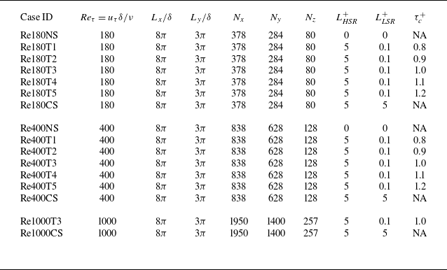


 Open access