


1. Introduction
The stability and transition of a high-speed boundary layer have been of great interest for more than half a century (Fedorov Reference Fedorov2011). Depending on the amplitude of environmental disturbances, there are multiple paths to turbulence in a boundary layer, e.g. eigenmode growth, transient growth and bypass mechanisms (Reshotko Reference Reshotko2008). However, in practical high-speed vehicles, the boundary layer on a surface frequently encounters shock waves generated by an adjacent or opposite surface (Gaitonde Reference Gaitonde2015). This shock-wave/boundary-layer interaction (SWBLI) can significantly alter the flow behaviour, e.g. causing boundary-layer separation. More importantly, the stability and transition mechanisms of the flow involving SWBLI can be essentially different to that of boundary-layer flows.
It is known that a separated flow has the potential to support self-excited instabilities (Theofilis Reference Theofilis2011). Therefore, for a strong SWBLI that undergoes boundary-layer separation, instabilities intrinsic to the separated flow may occur. The linear behaviour of the intrinsic instability can be described using global stability analysis (GSA). A flow is said to be globally unstable if a mode with positive temporal growth rate is found by the GSA. In this view, intrinsic instability and global instability are used interchangeably in the present paper to refer to the self-excited instability of a flow. As a canonical configuration involving SWBLI, compression-ramp flow serves as a suitable candidate for the study of the intrinsic instability of a separated flow.
Recently, Sidharth et al. (Reference Sidharth, Dwivedi, Candler and Nichols2017, Reference Sidharth, Dwivedi, Candler and Nichols2018) demonstrated the occurrence of intrinsic instability in supersonic flows over compression ramps by applying GSA. Beyond the stability boundary, the two-dimensional (2-D) separated flow was shown to bifurcate to stationary three-dimensional (3-D) perturbations taking the form of streamwise streaks (Sidharth et al. Reference Sidharth, Dwivedi, Candler and Nichols2018). Furthermore, when the instability is further enhanced by increasing the ramp angle, oscillatory unstable modes emerge (Sidharth et al. Reference Sidharth, Dwivedi, Candler and Nichols2018). By performing GSA for a compression-ramp flow at Mach 7.7, Cao et al. (Reference Cao, Hao, Klioutchnikov, Olivier and Wen2021b) revealed the existence of both stationary and oscillatory unstable modes in the separation bubble. They also conducted direct numerical simulations (DNS) and uncovered a low-frequency unsteadiness in the fully saturated flow. Furthermore, without introducing external disturbances in the DNS, Cao et al. (Reference Cao, Hao, Klioutchnikov, Wen, Olivier and Heufer2022) observed laminar–turbulent transition triggered by the intrinsic instability of a compression-ramp flow. It was shown that the intrinsic instability induces streamwise boundary-layer streaks and streamwise counter-rotating vortices downstream of reattachment, which then break down to turbulence. It should be mentioned that the self-excited instability has also been found in many separated flows associated with SWBLI, e.g. double-cone flow (Hao et al. Reference Hao, Fan, Cao and Wen2022), shock impingement on a flat plate (Robinet Reference Robinet2007; Hildebrand et al. Reference Hildebrand, Dwivedi, Nichols, Jovanović and Candler2018) and flow over a hollow cylinder/flare (Brown et al. Reference Brown, Boyce, Mudford and O'Byrne2009; Lugrin et al. Reference Lugrin, Beneddine, Garnier and Bur2021a).
Essentially, no matter whether an SWBLI is inherently unstable or stable, convective instabilities can play a role in destabilising the flow because external disturbances are usually present in ground experiments or during high-speed flights. Hence the transition paths applicable to boundary layers might be still valid in SWBLIs. For example, the propagation of second-mode disturbances in an incipiently separated flow over a double cone (Mach 6) was observed experimentally by Butler & Laurence (Reference Butler and Laurence2021). Lugrin et al. (Reference Lugrin, Beneddine, Leclercq, Garnier and Bur2021b) investigated numerically a transitional flow at Mach 5 over a hollow cylinder/flare, and found several possible transition paths, such as second mode, oblique mode and non-modal growth. Oblique transition in a hypersonic double-wedge flow was revealed by Dwivedi, Sidharth & Jovanović (Reference Dwivedi, Sidharth and Jovanović2022).
A remarkable phenomenon observed in compression-ramp experiments is the formation of streamwise heat-flux streaks on the ramp surface (Simeonides & Haase Reference Simeonides and Haase1995; Chuvakhov et al. Reference Chuvakhov, Borovoy, Egorov, Radchenko, Olivier and Roghelia2017; Roghelia et al. Reference Roghelia, Chuvakhov, Olivier and Egorov2017a,Reference Roghelia, Olivier, Egorov and Chuvakhovb; Chuvakhov & Radchenko Reference Chuvakhov and Radchenko2020). In addition to the intrinsic instability mentioned previously, convective mechanisms can also lead to the appearance of streamwise streaks. For instance, Roghelia et al. (Reference Roghelia, Chuvakhov, Olivier and Egorov2017a) reported two similar streak patterns obtained in the Aachen Shock Tunnel TH2 and the Ludwieg Wind Tunnel UT-1M under similar flow conditions. However, the compression-ramp flow studied in TH2 was shown to be intrinsically unstable (Cao et al. Reference Cao, Hao, Klioutchnikov, Olivier and Wen2021b), but the flow considered in UT-1M is dominated by convective instability (Dwivedi et al. Reference Dwivedi, Sidharth, Nichols, Candler and Jovanović2019). Therefore, one should pay attention to distinguishing the intrinsic and convective instabilities when explaining the observed streamwise streaks in a compression-ramp flow or other shock-induced separated flows.
Although the importance of convective instability in the formation of streamwise streaks has been confirmed, mechanisms responsible for the amplification of upstream disturbances are still under debate. The streamwise streaks are referred to conventionally as the footprint of Görtler-like vortices that are supported by the concave streamline curvature in the reattaching flow regions (Ginoux Reference Ginoux1971; de Luca et al. Reference de Luca, Cardone, de la Chevalerie and Fonteneau1995; de la Chevalerie et al. Reference de la Chevalerie, Fonteneau, de Luca and Cardone1997; Navarro-Martinez & Tutty Reference Navarro-Martinez and Tutty2005). However, recent studies (Zapryagaev, Kavun & Lipatov Reference Zapryagaev, Kavun and Lipatov2013; Dwivedi et al. Reference Dwivedi, Sidharth, Nichols, Candler and Jovanović2019) pointed out the importance of baroclinic effects. Dwivedi et al. (Reference Dwivedi, Sidharth, Nichols, Candler and Jovanović2019) examined the amplification of exogenous disturbances in a compression-ramp flow using a global input–output (I/O) analysis (also called resolvent analysis), and found that baroclinic effects arising from the interaction of upstream pressure perturbations with base-flow density gradients are responsible for the production of streamwise streaks.
Based on the above discussion, it is clear that in a compression-ramp experiment where external disturbances are present, there are usually two scenarios regarding flow instability. In the first circumstance, the compression-ramp flow is inherently stable (e.g. in an attached or weakly separated flow), and the convective instability makes the main contribution to destabilising the flow. Second, in an intrinsically unstable flow, both convective and intrinsic instabilities contribute to destabilising the flow. In our previous studies (Cao et al. Reference Cao, Hao, Klioutchnikov, Olivier and Wen2021b, Reference Cao, Hao, Klioutchnikov, Wen, Olivier and Heufer2022), it was shown that the intrinsic instability can lead independently to the formation of streamwise streaks and transition to turbulence. However, the influence of upstream disturbances on intrinsically unstable flows remains unknown. This is one of the motivations for the present study. In addition, the I/O analysis of Dwivedi et al. (Reference Dwivedi, Sidharth, Nichols, Candler and Jovanović2019) identified a low-pass frequency response feature (i.e. the dominant response is achieved for low-frequency inputs), although they studied mainly steady input perturbations. In the present work, we perform DNS and demonstrate that low-frequency streamwise streaks form on the ramp as a response to a white noise introduced upstream of the interaction region.
In order to study both the intrinsic and convective instabilities under the same flow conditions, it is convenient to modify the compression-ramp geometry. Instead of varying the ramp angle that changes the shock-induced pressure gradient, we propose to round the corner to alter directly the separation bubble flow while leaving the overall pressure gradient unchanged. In this work, stability analysis tools such as GSA, resolvent analysis and linear stability analysis are utilised to describe the stability of the considered flows. DNS are employed to study the two situations mentioned previously to gain a deeper understanding of the compression-ramp experiments.
The paper is organised as follows. Effects of corner rounding on the compression-ramp flow are presented in § 2. In § 3, GSA is conducted for the considered flows to identify the global stability. Then resolvent analysis is employed to examine the amplification of external disturbances for two selected cases in § 4. In § 5, DNS are performed to investigate the effects of external disturbances on intrinsically stable and unstable flows. A conclusion is provided in § 6.
2. Hypersonic flow over a curved compression ramp
2.1. Flow conditions and compression-ramp configuration
The flow considered in the present paper is based on the experimental work carried out at the Shock Wave Laboratory of RWTH Aachen University (Roghelia et al. Reference Roghelia, Chuvakhov, Olivier and Egorov2017a,Reference Roghelia, Olivier, Egorov and Chuvakhovb), which has been used widely in our previous studies (Cao et al. Reference Cao, Hao, Klioutchnikov, Olivier, Heufer and Wen2021a,Reference Cao, Hao, Klioutchnikov, Olivier and Wenb; Hao et al. Reference Hao, Cao, Wen and Olivier2021). As shown in table 1, the free-stream Mach number ( $M_\infty$) and unit Reynolds number ( $Re_{\infty }$) are 7.7 and $4.2\times 10^6$ m $^{-1}$, respectively. The total enthalpy $h_0$ is relatively low, allowing the use of the calorically perfect gas assumption. Owing to the short running time of the shock tunnel, the surface of the compression ramp is assumed isothermal, and the wall temperature ( $T_w$) is given as 293 K, which corresponds to a wall-to-total temperature ratio 0.18.
Flow conditions for the shock tunnel TH2 at RWTH Aachen University (Roghelia et al. Reference Roghelia, Olivier, Egorov and Chuvakhov2017b).
As mentioned previously, the intrinsic instability of a compression-ramp flow originates from the separation bubble. Hence it is viable to change the intrinsic instability by altering the separated flow. In the present study, we propose to use a curved corner to control the flow separation. Figure 1 demonstrates the geometry of a curved compression ramp. At the corner, a circular arc is used to connect the flat plate to the ramp, and it is tangential to both the flat plate and the ramp. With the turning angle of the compression ramp ( $\theta$) kept constant, the length of the circular arc (or the surface curvature) is determined by the tangent position. A reference case is introduced where the flat plate is connected to the ramp directly (i.e. without the circular arc). For this case, the length of the flat plate is set to $L = 100$ mm. For other cases, the distance from the leading edge of the flat plate to the tangent point is set to $L_t$. Five cases are considered here, namely $L_t/L = 1$, $0.9$, $0.8$, $0.77$ and $0.75$. For convenience, they are labelled as T100, T90, T80, T77 and T75, respectively, where T indicates the tangent point, and the number denotes the position of the tangent in mm. Obviously, case T100 corresponds to the reference case. For all cases, $\theta = 15^\circ$.
Geometry of a curved compression ramp.

2.2. Direct numerical simulations
The influence of corner rounding on the flow is investigated using DNS. The in-house DNS solver with shock-capturing ability features a finite-difference method of high-order accuracy in space and time. The Navier–Stokes equations for compressible flow are employed in a conservative form
 \begin{equation} \frac{\partial \boldsymbol{U}}{\partial t} + \frac{\partial \boldsymbol{F}}{\partial x} + \frac{\partial \boldsymbol{G}}{\partial y} + \frac{\partial \boldsymbol{H}}{\partial z} = \frac{\partial \boldsymbol{F}_\nu}{\partial x} + \frac{\partial \boldsymbol{G}_\nu}{\partial y} + \frac{\partial \boldsymbol{H}_\nu}{\partial z}, \end{equation}
where  $\boldsymbol{F}$, $\boldsymbol{G}$ and $\boldsymbol{H}$ are the inviscid fluxes, and $\boldsymbol{F}_\nu$, $\boldsymbol{G}_\nu$ and $\boldsymbol{H}_\nu$ denote the viscous fluxes. Here, $\boldsymbol{U} = (\rho, \rho u, \rho v, \rho w, \rho e)^{\rm T}$ is the vector of conservative variables, $\rho$ is the density, $u$,
$u$,  $v$ and $w$ are the flow velocities, and $e$ is the total energy per unit mass. The equation system is closed by the perfect gas law relating pressure, density and temperature (for the specific gas constant $R_{specific} = 287.1$ J ${\rm kg}^{-1}\ {\rm K}^{-1}$), as well as the following Sutherland's law for calculating the viscosity,
 \begin{equation} \mu = \mu_{ref} \left( \frac{T}{T_{ref}} \right)^{3/2} \frac{T_{ref} + S}{T + S},\end{equation}
where  $\mu _{ref} = 1.716 \times 10^{-5}$ kg ${\rm m}^{-1}\ {\rm s}^{-1}$, $T_{ref} = 273.15$ K, and $S = 110.4$ K. In addition, the specific heat ratio $\gamma$ and the Prandtl number $Pr$ used in the simulations are 1.4 and 0.72, respectively.
Regarding the numerical methods, time integration is performed by an explicit third-order total variation diminishing Runge–Kutta scheme. A weighted essentially non-oscillatory (WENO) scheme of fifth order is applied for the discretisation of the inviscid fluxes, based on the work of Jiang & Shu (Reference Jiang and Shu1996). A sixth-order central-difference scheme is used to approximate the viscous fluxes. Details about the numerical schemes may be found in Hermes, Klioutchnikov & Olivier (Reference Hermes, Klioutchnikov and Olivier2012), Cao et al. (Reference Cao, Hao, Klioutchnikov, Olivier and Wen2021b) and Cao (Reference Cao2021).
In 2-D simulations, the numbers of grid points in the streamwise ( $x$) and vertical ( $y$) directions are 1080 and 240, respectively. As shown in our previous studies for the same flow conditions (Cao Reference Cao2021; Cao et al. Reference Cao, Hao, Klioutchnikov, Olivier and Wen2021b), this mesh resolution is sufficient to capture the 2-D flow features. In terms of boundary conditions, free-stream parameters are prescribed at the inflow and upper boundaries. A zero-gradient extrapolation condition is used for the outflow boundary. For the no-slip wall, an isothermal condition is specified, with the temperature being 293 K.
Figure 2 shows the streamwise distribution of the skin friction coefficient ( $C_f$) for the considered cases. It is apparent that the separation and reattachment points are almost unchanged when the tangent point moves from $x/L = 1$ to $x/L = 0.77$. However, when the tangent point is located at
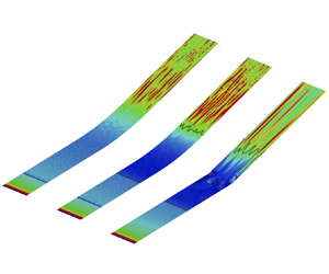
  $x/L = 0.75$, flow separation disappears, i.e. the boundary layer remains attached to the wall. The effects of surface curvature on the separation bubble flow are visualised in figure 3, which presents the Mach number contour for cases T100, T90, T77 and T75. Although the streamwise extent of the separation bubble is not affected as the tangent point moves from $x/L = 1$ to $x/L = 0.77$, the wall-normal extent is reduced. As a result, the recirculating flow in the separation bubble is altered.
Streamwise distribution of the skin friction coefficient for different cases.

Mach number contour for compression-ramp flow, for cases (a) T100, (b) T90, (c) T77, and (d) T75.

According to Hao et al. (Reference Hao, Cao, Wen and Olivier2021), global instability occurs prior to the appearance of secondary separation near the corner. As seen in figure 2, secondary separation is inhibited by the corner rounding. For example, secondary separation is present for case T100 but absent for cases T80 and T77. Therefore, it is conjectured that the intrinsic instability in the considered compression-ramp flow can be suppressed by using a properly curved surface at the corner. To verify this hypothesis, a GSA is employed to examine the intrinsic stability of the considered flows.
3. Global stability analysis
The current GSA considers the temporal stability of a 2-D base flow with respect to 3-D small-amplitude perturbations that are periodic in the spanwise direction. The linearised Navier–Stokes equations are given by
 \begin{equation} \frac{\partial \boldsymbol{U}'}{\partial t} + \frac{\partial \boldsymbol{F}'}{\partial x} + \frac{\partial \boldsymbol{G}'}{\partial y} + \frac{\partial \boldsymbol{H}'}{\partial z} = \frac{\partial \boldsymbol{F}'_\nu}{\partial x} + \frac{\partial \boldsymbol{G}'_\nu}{\partial y} + \frac{\partial \boldsymbol{H}'_\nu}{\partial z}, \end{equation}
where the prime represents perturbation variables. The governing equations can also be written in the operator form
 \begin{equation} \frac{\partial \boldsymbol{U}'}{\partial t} = \mathcal{A} \boldsymbol{U}',\end{equation}
where  $\mathcal{A}$ is the linearised Navier–Stokes operator. The perturbation $\boldsymbol{U}'$ is further assumed to be in the modal form
 \begin{equation} \boldsymbol{U}'(x,y,z,t) = \hat{\boldsymbol{U}}(x,y) \exp \left[ {\rm i}\,\frac{2{\rm \pi}}{\lambda}\,z - {\rm i}(\omega_r + {\rm i}\omega_i)t \right], \end{equation}
where  $\hat {\boldsymbol{U}}$ is the 2-D eigenfunction, $\lambda$ is the spanwise wavelength, $\omega _r$ is the angular frequency, and $\omega _i$ is the growth rate. Substituting (3.3) into (3.2) and discretising the result with the finite-volume method leads to the eigenvalue problem
 \begin{equation} \boldsymbol{\mathsf{A}} (\lambda)\hat{\boldsymbol{U}} ={-} {\rm i}(\omega_r + {\rm i}\omega_i)\hat{\boldsymbol{U}},\end{equation}
where  $\boldsymbol{\mathsf{A}}$ is the global Jacobian matrix, which is a function of $\lambda$. Note that the same symbol is used to denote both the eigenfunctions of operator $\mathcal {A}$ and the eigenvectors of matrix $\boldsymbol{\mathsf{A}}$.
In the discretisation, the inviscid fluxes are calculated using the modified Steger–Warming scheme (MacCormack Reference MacCormack2014) near discontinuities detected by a modified Ducros shock sensor (Hendrickson, Kartha & Candler Reference Hendrickson, Kartha and Candler2018) to suppress numerical noise, and using a central scheme in smooth regions to reduce numerical dissipation. The value of the shock sensor varies from 1 near shock waves to 0 elsewhere, and is used to evaluate an affine combination of the upwind and central fluxes. The viscous fluxes are computed with the second-order central difference. Specifically, a local transformation from Cartesian coordinates to the curvilinear coordinates is used to obtain the gradients of the velocity and temperature perturbations at the faces of a grid cell (Blazek Reference Blazek2015). A linear map from the primitive variables to the conservative variables is then applied. More computational details of the GSA solver can be found in Hao et al. (Reference Hao, Cao, Wen and Olivier2021).
The eigenvalue problem is solved using the implicitly restarted Arnoldi method implemented in ARPACK (Reference Sorensen, Lehoucq, Yang and MaschhoffSorensen et al. 1996–2008) for a given  $\lambda$ in the shift-invert mode. The inverse of matrix $\boldsymbol{\mathsf{A}}$ is obtained using the lower–upper decomposition implemented in SuperLU (Li et al. Reference Li, Demmel, Gilbert, Grigori, Shao and Yamazaki1999). The flow is globally unstable if an eigenvalue with $\omega _i > 0$ can be found.
Figure 4 compares the non-dimensional growth rates of the leading unstable mode as functions of  $\lambda$ for cases T100, T90, T80 and T77. The same grid resolution ( $700\times 300$ in the streamwise and wall-normal directions) is used for all the cases, which was verified to be sufficient in Hao et al. (Reference Hao, Cao, Wen and Olivier2021) for case T100. Note that the base flow of case T75 has no flow separation and thus supports no globally unstable mode. As reported in Hao et al. (Reference Hao, Cao, Wen and Olivier2021), the leading mode for case T100 has two peaks in growth rate that are stationary, that is, with zero $\omega _r$. As the corner is rounded, the short-wavelength peak is reduced significantly for case T90, and vanishes for cases T80 and T77. By contrast, the long-wavelength mode is first destabilised and then stabilised by corner rounding. For case T77, the maximum growth rate is close to that of the long-wavelength mode for case T100, although the flow is unstable over a wider range of $\lambda$. Due to the low growth rate, case T77 is believed to be more susceptible to convective instability than intrinsic instability, as seen later.
Growth rates of the leading unstable mode as functions of spanwise wavelength for cases T100, T90, T80 and T77.

4. Resolvent analysis
The current resolvent analysis considers the response of a 2-D globally stable base flow to external small-amplitude disturbances  $\boldsymbol{d}'$ that are periodic in time and in the spanwise direction. The corresponding linearised Navier–Stokes equations in operator form are given by
 \begin{equation} \frac{\partial \boldsymbol{U}'}{\partial t} = \mathcal{A} \boldsymbol{U}' + \mathcal{B} \boldsymbol{d}',\end{equation}
where operator  $\mathcal {B}$ constrains the forcing to a localised position, which is specified at $x/L = 0.2$ in accordance with the following DNS (see § 5), and $\boldsymbol{d}'$ is given by
 \begin{equation} \boldsymbol{d}'(x,y,z,t) = \hat{\boldsymbol{d}}(x,y) \exp \left( {\rm i}\,\frac{2{\rm \pi}}{\lambda}\,z - i \omega_r t \right). \end{equation}
Note that all initial perturbations imposed on a globally stable base flow decay to zero as time approaches infinity. In other words, the long-time solution of (4.1) takes the same form as the forcing, which is given by
 \begin{equation} \boldsymbol{U}'(x,y,z,t) = \hat{\boldsymbol{U}}(x,y) \exp \left( {\rm i}\,\frac{2{\rm \pi}}{\lambda}\,z - {\rm i} \omega_r t \right). \end{equation}
Substituting (4.2) and (4.3) into (4.1), and discretising the result in the same way as in the GSA, gives
 \begin{equation} \hat{\boldsymbol{U}} = \boldsymbol{\mathsf{R}}\boldsymbol{\mathsf{B}}\hat{\boldsymbol{d}},\quad \boldsymbol{\mathsf{R}} = (-{\rm i}\omega_r \boldsymbol{\mathsf{I}} - \boldsymbol{\mathsf{A}})^{{-}1},\end{equation}
where  $\boldsymbol{\mathsf{R}}$ is the resolvent matrix, $\boldsymbol{\mathsf{B}}$ is the constraint matrix, and $\boldsymbol{\mathsf{I}}$ is the identity matrix.
The resolvent analysis seeks the forcing and response pair that maximises the energy amplification defined by
 \begin{equation} \sigma^2(\lambda,\omega_r) = \max_{\hat{d}} \frac{\|\hat{\boldsymbol{U}}\|_E}{\|\boldsymbol{\mathsf{B}}\hat{d}\|_E}, \end{equation}
where  $\sigma$ is the optimal gain, and the energy norm is evaluated based on the Chu energy (Chu Reference Chu1965). Note that (4.5) holds only if the denominator is non-zero. According to Sipp & Marquet (Reference Sipp and Marquet2013), Bugeat et al. (Reference Bugeat, Chassaing, Robinet and Sagaut2019) and Dwivedi et al. (Reference Dwivedi, Sidharth, Nichols, Candler and Jovanović2019), the optimisation problem (4.5) can be converted to an eigenvalue problem as
 \begin{equation} \boldsymbol{\mathsf{B}}^* \boldsymbol{\mathsf{M}}^{{-}1} \boldsymbol{\mathsf{R}}^{*-1} \boldsymbol{\mathsf{M}}\boldsymbol{\mathsf{R}}^{{-}1} \boldsymbol{\mathsf{B}} \hat{\boldsymbol{d}} = \sigma^2 \hat{\boldsymbol{d}}, \end{equation}
where the superscript  $*$ denotes the complex conjugate, and $\boldsymbol{\mathsf{M}}$ is the weight matrix to calculate the Chu energy (Bugeat et al. Reference Bugeat, Chassaing, Robinet and Sagaut2019). Consistent with the GSA, the current resolvent analysis is formulated in terms of the conservative variables. One may refer to Karban et al. (Reference Karban, Bugeat, Martini, Towne, Cavalieri, Lesshafft, Agarwal, Jordan and Colonius2020) for an ambiguity in the results depending on whether the analysis is performed using the primitive or conservative variables, although they considered turbulent flow. The eigenvalue problem is solved using ARPACK in the regular mode. The largest eigenvalue and the corresponding eigenvector represent the square of the optimal gain and the optimal forcing, respectively. The optimal response is then obtained using (4.4).
Figure 5 compares the contours of the optimal gain in the space of  $\lambda$ and $\omega _r$ for cases T77 and T75. Here, $\lambda /L$ ranges from 0.00628 to 0.1, and $\omega _r L/U_\infty$ ranges from 0.1 ( $f$ = 278 Hz) to 100 ( $f$ = 278 kHz). As seen in figure 4, the base flows are globally stable in the considered range of $\lambda$. For both cases, the maximum optimal gain is achieved at $\lambda /L \approx 0.021$ as the forcing frequency approaches zero. In fact, the optimal gain is insensitive to the forcing frequency for $\omega _r L/U_\infty < 10$ ( $f < 27$ kHz). Such a low-pass feature was also observed in hypersonic compression-ramp flow (Dwivedi et al. Reference Dwivedi, Sidharth, Nichols, Candler and Jovanović2019) and shock impingement on a supersonic boundary layer (Bugeat et al. Reference Bugeat, Robinet, Chassaing and Sagaut2022). By comparing cases T77 and T75, flow separation is found to increase slightly the maximum optimal gain by a factor of 1.6, while the preferential spanwise wavelength is largely unchanged.
Contours of optimal gain in the space of  $\lambda$ and $\omega _r$ for cases (a) T77, and (b) T75.

Figure 6 presents the most amplified optimal forcing and response pairs at  $\lambda /L = 0.021$ and $\omega _r L/U_\infty = 0.1$ for cases T77 and T75. For both cases, the forcing is in the form of counter-rotating streamwise vortices ( $|u'| \ll |v'|$ and $|u'| \ll |w'|$), while the responses are streamwise streaks ( $|u'| \gg |v'|$ and $|u'| \gg |w'|$). Note that only the contours of $|u'|$ are shown for the responses. Such a componentwise energy transfer, also known as the lift-up mechanism (Landahl Reference Landahl1980), is responsible for the transient growth of the streamwise streaks over the flat plate. Further downstream, the streamwise streaks experience strong amplification in the shear layer above the separation bubble for case T77, and over the circular arc for case T75. Figure 7 shows the distributions of the Chu energy density (i.e. the Chu energy per unit volume) integrated in the wall-normal direction for cases T77 and T75. For case T75 with no flow separation, the spatial growth over the circular arc is nearly exponential, which indicates the well-known Görtler instability (Spall & Malik Reference Spall and Malik1989; Floryan Reference Floryan1991; Saric Reference Saric1994) due to wall curvature. By contrast, the effective wall shape of case T77 is altered by the separation bubble such that high streamline curvature is associated with the separation and reattachment processes. Therefore, the continuous growth over the circular arc as in case T75 is replaced by two separate stages. In short, the resolvent analysis confirms that the dynamics of cases T77 and T75 with respect to upstream disturbances are similar, and the separation bubble contributes little to the amplification of the streamwise streaks in the interaction region.
(a,b) Optimal forcings and (c,d) responses associated with the most amplified streamwise streaks at  $\lambda /L = 0.021$ and $\omega _r L/U_\infty = 0.1$ for cases T77 and T75. Open circles indicate separation and reattachment points, and tangent points; black dashed lines indicate the edge of the boundary layer at $x/L = 0.2$; black solid lines indicate dividing streamlines and solid wall.

Distributions of Chu energy density integrated in the wall-normal direction associated with the most amplified streamwise streaks at  $\lambda /L = 0.021$ and $\omega _r L/U_\infty = 0.1$ for cases T77 and T75. Open circles indicate separation and reattachment points, and points of tangency.

5. DNS of compression-ramp flows subject to external disturbances
As revealed by the resolvent analysis, for cases T77 and T75, the flow strongly amplifies low-frequency upstream disturbances and produces streamwise streaks on the ramp. Towards this end, 3-D simulations are first performed for cases T77 and T75 to demonstrate the presence of streamwise streaks and verify the predicted frequencies and wavelengths. Subsequently, upstream disturbances are introduced for the intrinsically unstable flow (case T100) to examine the combined effects of convective and intrinsic instabilities.
The initial 3-D flow field is generated by extending the 2-D solution in § 2 in the spanwise direction ( $z$). 120 grid points are equispaced in spanwise length 20 mm for cases T77 and T75, and 19.8 mm for case T100. Note that the resulting mesh resolution ( $1080\times 240\times 120$) is slightly higher than that used in our previous study for case T100 (Cao et al. Reference Cao, Hao, Klioutchnikov, Olivier and Wen2021b). Nevertheless, a grid-independence study for case T77 is carried out (see Appendix A). Periodic boundary conditions are applied at the spanwise boundaries.
Instead of imposing a ‘controlled’ mode with specific frequency and wavelength, a random forcing is introduced here to excite broadband upstream disturbances. As demonstrated by Hader & Fasel (Reference Hader and Fasel2018), this enables us to study the ‘natural’ transition process observed in wind tunnel experiments when detailed information regarding free-stream disturbances is not available. This idea is also considered by Lugrin et al. (Reference Lugrin, Beneddine, Leclercq, Garnier and Bur2021b) to study the transition scenario in an axisymmetrical compression-ramp flow. In the present study, the random forcing is introduced upstream of flow separation taking the form
 \begin{equation} w^{\prime}_{j,k}/U_\infty = A_{noise}(2r-1),\end{equation}
where the indices  $j$ and $k$ refer to the grid point indices in the $y$ and $z$ directions, respectively, $A_{noise}$ is the amplitude of perturbations, and $r$ represents a pseudo-random number (ranging from 0 to 1) generated by the rand() function in C. Specifically, random spanwise velocity perturbations with noise level $A_{noise} = 0.1$ are imposed on the $y$–
$y$– $z$ plane at $x/L = 0.2$ (i.e. for $1 \leqslant j \leqslant 240$ and $1 \leqslant k \leqslant 120$). This noise level was chosen for two reasons. First, the induced disturbances decay rapidly downstream on the flat plate, as shown later. Second, the chosen noise level makes the magnitude of the heat-flux streaks induced by convective instability comparable to that of the heat flux measured in experiments (see § 5.3). It should be noted that the resulting magnitude of the surface heat flux is highly dependent on the noise level. To ensure a sufficient time for the convection of disturbances through grid points, the perturbation is updated every 50 time steps, not at each time step. This yields a time interval $1.74 \times 10^{-7}$ s (or ${\rm \Delta} t\,U_\infty /L = 0.003$) for updating the spanwise velocity. Accordingly, the DNS data are sampled using the same time interval, leading to sampling frequency $f_s = 5.75$ MHz (or $f_sL/U_\infty = 333$).
In the following, spectral analysis is performed for the random forcing and the excited disturbances. Note that the forcing and the induced disturbances are statistically the same for all three cases. A time period 1 ms ( $tU_\infty /L = 18$) is monitored. It should be mentioned that the data were recorded after the initial transient flow has been convected out of the computational domain. Figure 8(a) shows the temporal history of $w'/U_\infty$ at a grid point ( $j = 60$, $k = 60$) inside the boundary layer at $x/L = 0.2$. As expected, random values ranging from $-$0.1 to 0.1 are introduced at this point. Figure 8(b) provides the frequency spectrum for this signal. Welch's method (Welch Reference Welch1967) is employed for the spectral estimation with three segments and 50 % overlap. A Hamming window is used for weighting the data on each segment prior to fast Fourier transform (FFT) processing. The resulting spectrum exhibits a broadband feature as intended. Figures 8(c) and 8(d) present the induced pressure disturbance ( $p' /p_\infty$) at $x/L = 0.2$ ( $j=1$, $k=60$) and the frequency spectrum of this wall pressure signal, respectively. Similar to the spanwise velocity, the induced pressure disturbances also have a broadband spectrum. Analogously, it is easy to prove that the forcing and the induced disturbances have a wide range of spanwise wavelengths. Therefore, while using the random forcing, we do not choose a mode with specific frequency and wavelength, but let the flow select the preferred mode from the disturbances. This is a suitable way to verify the resolvent analysis results, and represents a situation that is likely to happen in wind tunnel experiments.
(a) Temporal history of spanwise velocity at  $x/L = 0.2$ ( $j = 60$, $k = 60$). (b) Power spectral density (PSD) of the signal in (a). (c) Temporal history of pressure perturbation at $x/L = 0.2$ ( $j=1$, $k = 60$). (d) PSD of the signal in (c).

As the disturbances are convected downstream, they decay rapidly. Figure 9 shows the temporal history of the spanwise velocity and pressure perturbations at  $x/L = 0.3$. It is apparent that the amplitude of both disturbances drops dramatically. For instance, the root-mean-square value of the spanwise velocity signal reduces from 0.058 at $x/L = 0.2$ (figure 8a) to 0.002 at $x/L = 0.3$ (figure9a). Furthermore, in the spanwise velocity signal, the low-frequency component is more energetic than the high-frequency component, which is common in flat plate boundary layer flows (Ran et al. Reference Ran, Zare, Hack and Jovanović2019). Interestingly, the PSD of pressure signal peaks at $f \approx 400$ kHz (see figure 9d). This frequency compares well with the dominant frequency of the second-mode instability for the boundary-layer profile at $x/L = 0.3$, as demonstrated in Appendix B by using linear stability theory (LST).
(a) Temporal history of spanwise velocity at  $x/L = 0.3$ ( $j = 60$, $k = 60$). (b) PSD of the signal in (a). (c) Temporal history of pressure perturbation at $x/L = 0.3$ ( $j=1$, $k = 60$). (d) PSD of the signal in (c). The dashed line in (d) represents the dominant frequency of the second-mode instability for the local boundary layer, which is obtained using linear stability theory (LST).

5.1. Effects of external disturbances on an attached flow
Next, the emergence of streamwise streaks for case T75 is examined. As shown in § 2, flow separation is absent for this case. However, streamwise heat-flux streaks are captured by DNS while adopting the above random forcing. Figure 10 shows instantaneous wall Stanton number distributions at  $tU_\infty / L = 12$ and 18. The wall Stanton number is defined as
 \begin{equation} St = \frac{q_w}{\rho_\infty U_\infty c_p (T_{aw}-T_w)}, \end{equation}
where  $q_w$ denotes the surface heat flux, $c_p$ is the specific heat capacity, and $T_{aw}$ is the adiabatic wall temperature. Streamwise heat-flux streaks can be observed on the ramp surface. However, their spatial distributions are not identical at the two instants, indicating an unsteady streak pattern over the ramp.
Instantaneous distributions of wall Stanton number for case T75 at (a)  $tU_\infty / L = 12$, and (b) $tU_\infty / L = 18$.

To further examine the unsteadiness of the streamwise streaks, the  $St$ signal at $(x/L, z/L) = (1.5, 0.1)$ together with its frequency spectrum are provided in figure 11. While a local peak corresponding to the second-mode instability exists at $f \approx 800$ kHz (see Appendix B), low-frequency components dominate the signal. The above facts confirm the previous resolvent analysis results that the optimal response takes the form of low-frequency streamwise streaks, and the optimal gain is nearly the same for forcing frequencies less than 27 kHz.
(a) Temporal history of wall Stanton number at  $(x/L, z/L) = (1.5, 0.1)$ for case T75. (b) PSD of the signal in (a).

In terms of the spanwise wavelength of the streaks, figure 12 presents the PSD of the spanwise distribution of  $St$ at $x/L = 1.3$ for case T75. Note that the plot is obtained by averaging the FFT results at all time instants. The preferential wavelength of the heat-flux streaks is in the range $\lambda /L = 0.02\unicode{x2013}0.03$, which covers the wavelength for the most amplified streamwise streaks predicted by the resolvent analysis.
PSD of the spanwise variation of  $St$ at $x/L = 1.3$ for case T75.

5.2. Effects of external disturbances on a separated flow
Subsequently, the influence of external disturbances on case T77 is discussed. As revealed by the GSA, case T77 does not support the short-wavelength unstable mode (see figure 4). Although there exists a long-wavelength unstable mode, its temporal growth rate is extremely low, indicating a long simulation time and huge computational cost. Preliminary simulation showed that for a time period  $tU_\infty /L = 30$, the initial flow field remains 2-D in the absence of external disturbances. Owing to the short width of the physical domain (20 mm) and the short simulation time, case T77 can be viewed as a globally stable flow. In other words, the long-wavelength global mode is not considered in the present numerical simulation. This allows us to study the individual role of convective instability.
By introducing the random forcing at  $x/L = 0.2$, and after the initial transient is convected out, the DNS capture streamwise streaks downstream of reattachment. Figure 13 shows the distribution of wall Stanton number at two time instants for case T77. Like case T75, unsteady heat-flux streaks can be observed on the ramp surface. Note that the meandering reattachment line is caused by the distorted reattaching shear layer (Cao, Klioutchnikov & Olivier Reference Cao, Klioutchnikov and Olivier2019).
Instantaneous distributions of wall Stanton number for case T77 at (a)  $tU_\infty / L = 12$, and (b) $tU_\infty / L = 18$. Black solid lines denote iso-lines of $C_f = 0$.

Figure 14(a) presents the wall Stanton number signal at  $(x/L, z/L) = (1.5, 0.1)$. The corresponding frequency spectrum is given in figure 14(b). Consistent with previous resolvent analysis, the surface heat flux is characterised by a low-frequency unsteadiness, and the dominant amplitude is found for $f < 27$ kHz. Additionally, a local peak can be found at approximately 800 kHz, which is close to the dominant frequency of the second-mode instability at this position (see Appendix B for more details).
(a) Temporal history of wall Stanton number at  $(x/L, z/L) = (1.5, 0.1)$ for case T77. (b) PSD of the signal in (a).

The spanwise wavelength of the heat-flux streaks is then examined by performing an FFT for the spanwise distribution of  $St$ near reattachment (at $x/L = 1.3$). Figure 15 presents the time-averaged PSD as a function of spanwise wavelength. Similar to case T75, the heat-flux streaks have a dominant spanwise wavelength for $\lambda /L = 0.02\unicode{x2013}0.03$. Therefore, it seems that the presence of a separation bubble does not alter the selected spanwise wavelength, which is consistent with the previous resolvent analysis and in contrast to the result of Dwivedi et al. (Reference Dwivedi, Sidharth, Nichols, Candler and Jovanović2019).
PSD of the spanwise variation of  $St$ at $x/L = 1.3$ for case T77.

In short, the above DNS results corroborate that in an intrinsically stable compression-ramp flow, the amplification of the disturbances generated by a random forcing leads to low-frequency streamwise streaks with a specific spanwise wavelength. On the other hand, in some compression-ramp experiments, both intrinsic and convective instabilities may play a role in the formation of streamwise streaks owing to the presence of environmental noise (e.g. free-stream turbulence). Towards this end, the effects of external disturbances on an intrinsically unstable flow are investigated in the following.
5.3. Effects of external disturbances on an intrinsically unstable flow
According to § 3 and Cao et al. (Reference Cao, Hao, Klioutchnikov, Olivier and Wen2021b), case T100 is characterised by the intrinsic instability that triggers low-frequency streamwise streaks downstream of reattachment. To examine the influence of external disturbances on the streamwise streaks triggered by the intrinsic instability, the same random forcing as used for cases T75 and T77 is introduced for case T100. The numerical simulation process is as follows.
In the 3-D simulation for case T100, the spanwise length of the physical domain is set to 19.8 mm, which is three times the wavelength of the most unstable global mode. Owing to the intrinsic instability, the initial flow bifurcates to three-dimensionality and then saturates to a quasi-steady state. Hence the first step is to run a simulation up to  $tU_\infty /L = 60$ to obtain a saturated flow in the absence of external disturbances. Based on our previous results (Cao et al. Reference Cao, Hao, Klioutchnikov, Olivier and Wen2021b), this intrinsically unstable flow can reach a quasi-steady state prior to $tU_\infty /L = 60$. Then two simulations are performed simultaneously. In the first case, the simulation without external disturbances is continued. The obtained flow is used for comparison. In the second simulation, the random forcing is imposed at $x/L = 0.2$. After some flow-through time, a fully developed flow subject to both intrinsic and convective instabilities is obtained. It should be mentioned that the timing of introducing external disturbances has no significant influence on the behaviour of heat-flux streaks in the fully saturated flow because both convective and intrinsic instabilities induce low-frequency streamwise streaks downstream of reattachment.
The unsteadiness of these two flows is compared below. Figure 16 shows the instantaneous wall Stanton number distributions (at  $tU_\infty /L = 75$) in the absence and presence of external disturbances. It seems that the spanwise wavelength of the heat-flux streaks is reduced after introducing upstream disturbances. In addition to the large-scale streaks, small-scale heat-flux variation in the streamwise direction can be observed in figure 16(b), which resembles the heat-flux distribution for case T77 (figure 13).
Instantaneous ( $tU_\infty /L = 75$) distributions of wall Stanton number for case T100 in (a) the absence and (b) the presence of external disturbances.

Figure 17(a) presents the wall Stanton number signal (at  $tU_\infty /L = 66 \sim 84$) for the flows with and without external disturbances. The corresponding frequency spectra are shown in figure 17(b). Although both flows are unsteady, the surface heat flux exhibits a broader frequency spectrum after introducing upstream disturbances. Specifically, in the flow without forcing, the dominant frequency is in the range 0–8 kHz. However, in the presence of external disturbances, the dominant amplitude can be found for $f < 30$ kHz. It is noted that although resolvent analysis is not applicable for case T100, the flow structure upstream and downstream of the separation bubble is nearly the same in the base flow for cases T77 and T100. As a result, when external disturbances are introduced, the frequency spectrum of $St$ for case T100 resembles that for case T77 (see figures 14b and 17b).
(a) Temporal history of wall Stanton number at  $(x/L, z/L) = (1.5, 0.1)$ for case T100. (b) PSD of the signal in (a). Solid and dashed lines correspond to the flow with and without external disturbances, respectively.

The spanwise wavelength of heat-flux streaks is then compared for the two flows in figure 18. In the absence of external disturbances, the dominant wavelengths are concentrated around  $\lambda /L = 0.045$. However, the dominant wavelengths extend to a lower range when external disturbances are introduced. Although resolvent analysis is not applicable for case T100, the preferential wavelength selected by the convective instability is expected to be close to that of case T77, namely, $\lambda /L \approx 0.021$. Therefore, a combination of intrinsic and convective instabilities tends to make a wider wavelength range for the streamwise streaks.
PSD of the spanwise variation of  $St$ at $x/L = 1.3$ for case T100. Solid and dashed lines correspond to the flow with and without external disturbances, respectively.

Next, the evolution of surface heat flux induced by the instabilities is discussed. Figure 19 plots the streamwise distributions of  $St$ for case T100 obtained from both 2-D and 3-D simulations. Also shown are the experimental data from Roghelia et al. (Reference Roghelia, Olivier, Egorov and Chuvakhov2017b). Note that the uncertainty of heat-flux measurement in the shock tunnel experiment is 10 % (Roghelia et al. Reference Roghelia, Olivier, Egorov and Chuvakhov2017b). When external disturbances are absent, i.e. only intrinsic instability takes effect, the heat flux on the ramp surface is larger than the 2-D result owing to the occurrence of streamwise streaks, but it is smaller than the experimental result. After introducing upstream disturbances, the surface heat flux is elevated further. For instance, the heat transfer rises by approximately 34 % at $x/L = 1.5$ compared to the flow without forcing. More importantly, a better comparison to the experimental result is achieved in the presence of upstream disturbances. Hence the DNS results indicate that both convective and intrinsic instabilities play a role in destabilising the experimentally studied compression-ramp flow. This is reasonable because environmental noise usually exists in experiments conducted in supersonic wind tunnels (Laufer Reference Laufer1961).
Streamwise distributions of  $St$ for case T100 in comparison with experimental result (Roghelia et al. Reference Roghelia, Olivier, Egorov and Chuvakhov2017b). The black and red lines correspond to the spanwise-averaged value at $tU_\infty /L = 75$.

In summary, the above numerical simulations represent two typical scenarios that could be encountered in experiments: (1) a compression-ramp flow dominated by convective instability (cases T75 and T77); (2) a compression-ramp flow affected by both convective and intrinsic instabilities (case T100). In both scenarios, the flows are characterised by low-frequency streamwise streaks. On the one hand, the similar flow pattern may bring difficulties in explaining experimental results, as discussed in the Introduction. On the other hand, although the streamwise streaks in the two scenarios resemble each other, their magnitude, frequency and spanwise wavelength are dependent on the associated instabilities, which complicates the transition process.
6. Conclusion
In this work, the stability of hypersonic flow over a curved compression ramp was investigated using several stability analysis tools as well as DNS. The free-stream Mach number and the Reynolds number based on the flat plate length are 7.7 and  $4.2 \times 10^5$, respectively. A circular arc that is tangent to both the flat plate and the ramp was used to alter the intrinsic stability of the compression-ramp flow.
GSA was first performed to identify the stability intrinsic to the considered flows. As the tangent point moves upstream, the size of the separation bubble reduces, and the flow tends to be more stable. At a critical corner curvature, the separation bubble disappears. Consequently, the intrinsic instability is inhibited by the corner rounding.
Subsequently, resolvent analysis was employed to examine the response of intrinsically stable flows to external disturbances. It was shown that for cases T77 and T75, the flow strongly amplifies low-frequency streamwise streaks with a preferential spanwise wavelength. Moreover, the streamwise streaks arise from the transient growth over the flat plate, and experience significant amplification in regions with large streamline curvature.
The resolvent analysis results were then verified using DNS. While imposing a random forcing (white noise) at  $x/L = 0.2$ for cases T77 and T75, unsteady streamwise heat-flux streaks were observed on the ramp surface. Consistent with the resolvent analysis results, the streamwise streaks exhibit a low-frequency feature and have a specific spanwise wavelength. In addition, both the resolvent analysis and DNS confirmed that the separation bubble contributes little to the selection of the spanwise wavelength of the streaks.
The influence of external disturbances on an intrinsically unstable flow was also studied using DNS. Introducing the random forcing for case T100 results in a broader frequency spectrum and a wider wavelength range for the streamwise streaks. However, a better comparison to the experimental data regarding the surface heat flux downstream of reattachment is achieved in the presence of external disturbances, which indicates that both convective and intrinsic instabilities may play a role in destabilising the compression-ramp flow in the experiment.
As environmental noise is usually present in experiments conducted in wind tunnels, convective instability can be dominant in an intrinsically stable flow. On the other hand, an intrinsically unstable flow can also be subject to convective instability. Their combined effects may enhance the transition process. Therefore, the present study contributes to understanding these two scenarios that can promote transition to turbulence in a hypersonic compression-ramp flow. It should be noted that the forcing amplitudes are chosen arbitrarily in this work. A thorough and precise comparison between numerical simulation and experiment requires accurate information of the wind tunnel noise.
Funding
This work was supported by the Hong Kong Research Grants Council (no. 25203721) and the National Natural Science Foundation of China (no. 12102377).
Declaration of interests
The authors report no conflict of interest.
Appendix A. Grid-independence study for case T77
A grid-independence study is conducted for case T77. Two mesh resolutions,  $1080 \times 240 \times 120$ and $1890 \times 320 \times 200$, are considered. A random forcing in the form of (5.1) is introduced at $x/L = 0.2$ to excite upstream disturbances. As a consequence, streamwise heat-flux streaks form on the ramp surface downstream of reattachment. Figure 20(a) shows the streamwise distribution of spanwise-averaged $St$ at a time instant. The spanwise distribution of $St$ at $x/L = 1.5$ is given in figure 20(b). It is obvious that the length of the separation bubble and the heat-flux level both inside and downstream of the separation bubble are nearly the same for the two mesh resolutions. Moreover, the spanwise wavelength of the heat-flux streaks is approximately 2 mm for both mesh resolutions. Therefore, the mesh resolution $1080 \times 240 \times 120$ is shown to be sufficient to capture the streamwise streaks triggered by the convective instability.
(a) Streamwise distribution of spanwise-averaged  $St$, and (b) spanwise distribution of $St$ at $x/L = 1.5$, for case T77 with two mesh resolutions: $1080 \times 240 \times 120$ (black) and $1890 \times 320 \times 200$ (red).

Appendix B. LST analysis
The present linear stability analysis considers the convective instability problem in a compressible boundary layer induced by a small-amplitude disturbance. The form of disturbance is assumed as
 \begin{equation} \boldsymbol{\phi}' (x,y,z,t) = \boldsymbol{\varphi}(y)\,{\rm e}^{\text{i}(\alpha x + \beta z - \omega t)} + \text{c.c.}, \end{equation}
where  $\boldsymbol{\varphi} = (\hat \rho,\hat u,\hat v,\hat w,\hat T)^{\rm {T}}$ is the eigenfunction, and $\alpha = \alpha _r + \text {i} \alpha _i$, with ${\alpha }_r$ the streamwise wavenumber, and $-{\alpha }_i$ the spatial growth rate. The symbols $\beta$ and $\omega$ denote the spanwise wavenumber and the angular frequency, respectively, and c.c. refers to the complex conjugate. With the introduction of the parallel-flow assumption, the linearised Navier–Stokes equations are transformed into an LST eigenvalue problem. This is subsequently solved by a Chebyshev pseudo-spectral method to obtain the global eigenvalue spectrum and an iterative compact fourth-order difference scheme to improve the accuracy of the eigenvalue and eigenfunction (Malik Reference Malik1990). The present LST code has been validated by calculating a series of benchmark cases (Guo et al. Reference Guo, Gao, Jiang and Lee2020, Reference Guo, Gao, Jiang and Lee2021). The base flow is provided by the present DNS solver, and the wall-normal pressure gradient of the base flow is included in the LST analysis. For the calculation of the most unstable second mode, the spanwise wavenumber is set to zero. Figure 21 shows the spatial growth rate varying with the frequency at three different positions. The corresponding most pronounced frequencies are used for the comparisons with the DNS energy spectra (see figures 9d, 11b and 14b). In addition to the analysis for the second Mack mode ( $\beta = 0$), LST analysis with non-zero spanwise wavenumber is also performed for the boundary-layer profiles at $x/L = 0.3$ and 0.5. It is found that the Mach 7.7 cold-wall boundary layer does not support the first Mack mode.
Variation of the spatial growth rate with the frequency for the most unstable second mode.


 Open access