3. Results and discussion

We begin by presenting the lift fluctuation for the $G=2$ case in the laminar and turbulent regimes. In figure 2 $(a)$ , the light and dark red lines represent the lift histories for ${\textit{Re}}=600$ and 10 000, respectively. The lift coefficient is defined as $C_L=F_L/(( {1}/{2}) \rho u_\infty ^2 bc)$ , where $F_L$ is the lift force on the wing, $\rho$ is the fluid density and $b$ is the span length. Before the gust vortex is introduced in the flowfield, the flow is steady at ${\textit{Re}}=600$ with $C_{L,{base}}=0.22$ , while it is unsteady at ${\textit{Re}}=$ 10 000 with a time-averaged lift coefficient of $\bar {C}_{L,{base}}=0.32$ . As the gust vortex approaches the wing, the wing experiences a substantial lift increase, which peaks at $\tau =\tau _1$ for both ${\textit{Re}}=600$ and 10 000. After the positive peak, the lift drops and reaches its negative peak at $\tau =\tau _2$ . Subsequent to these lift fluctuations, the lift recovers to the baseline values.

Figure 2. (a) Lift history for the $G=2$ case at ${\textit{Re}}=600$ (light red) and 10 000 (dark red). (b) Top-port view of the Q-criterion isosurface $Q=10$ , coloured in grey, at $\tau =\tau _1$ and $\tau _2$ noted in panel (a). The Q-criterion isosurface $Q=10$ of the large-scale structures extracted by the scale decomposition analysis with $\sigma /c=0.05$ in the ${\textit{Re}}=$ 10 000 case is superposed in green.

The time evolution of the vortex cores is presented in figure 2 $(b)$ , where we visualise the Q-criterion isosurface at ${\textit{Re}}=600$ and 10 000 in grey. For the ${\textit{Re}}=$ 10 000 case, the Q-criterion isosurface of large-scale structures extracted through scale decomposition (Motoori & Goto Reference Motoori and Goto2019; Fujino et al. Reference Fujino, Motoori and Goto2023) is also visualised in green, where we decompose a velocity component $u_i$ into the large-scale $\widetilde {u}_{i_L}$ and the small-scale $\widetilde {u}_{i_S}$ by applying a Gaussian filter $K$ in three spatial directions such that

(3.1) \begin{align} &\widetilde {u}_{i_L}(x,y,z; \sigma ) = \sum _{x_p}\sum _{y_p}\sum _{z_p} u_i(x_p,y_p,z_p) K(x_p,y_p,z_p;x,y,z), \end{align}

(3.2) \begin{align} &\widetilde {u}_{i_S}(x,y,z; \sigma ) = u_i - \widetilde {u}_{i_L}(x,y,z; \sigma ). \end{align}

Here, $x_p$ , $y_p$ and $z_p$ are the coordinates of grid points. The Gaussian kernel is

(3.3) \begin{equation} K(x_p,y_p,z_p;x,y,z)= C(x,y,z) \exp { \left [\!-\frac {(x_p-x)^2+(y_p-y)^2+(z_p-z)^2}{2\sigma ^2}\!\right ]} \Delta x \Delta y \Delta z \end{equation}

and the coefficient $C(x,y,z)$ is selected to ensure the sum of the kernel is unity;

(3.4) \begin{equation} \sum _{x_p}\sum _{y_p}\sum _{z_p} K(x_p,y_p,z_p;x,y,z)=1. \end{equation}

Parameter $\sigma$ is the effective size of the Gaussian filter, where information approximately smaller than $\sigma$ is smoothed out in the filtered velocity $\widetilde {u_i}_{|L}$ (Motoori & Goto Reference Motoori and Goto2019). Here, $\sigma /c=0.05$ is chosen to uncover the large-scale vortical structures that are primarily responsible for the lift peaks, shown in figure 2 $(b)$ . The influence of $\sigma /c$ is examined later.

As shown in figure 2 $(b)$ , the large-scale flow structures between the laminar and turbulent flows are strikingly similar. At the first lift peak $\tau =\tau _1$ , we observe the development of a large leading-edge vortex (LEV) for both ${\textit{Re}}=600$ and 10 000. This results from a substantial amount of gust-induced wall-normal vorticity production at the leading edge (Taira Reference Taira2026). Notably, these accentuated vorticity production levels at the leading edge are directly related to the enhanced surface pressure gradients caused by the incoming gust vortex (Lopez-Doriga, Jones & Taira Reference Lopez-Doriga, Jones and Taira2025). During the gust–leading-edge interaction, which is up until the impingement, viscous effects are not prominent (Peng & Gregory Reference Peng and Gregory2015) and similar large-scale topological features are observed across the two Reynolds numbers. Even at ${\textit{Re}}=$ 10 000, the locally accelerated flow near the leading edge experiences stabilising effects (Linot, Schmid & Taira Reference Linot, Schmid and Taira2024), producing large-scale, laminar flow structures.

Furthermore, the tip vortices (TiVs) grow in size near the leading edge for both Reynolds-number flows during the encounter. This is because the impacting gust vortex induces a large vorticity flux at the tip near the leading edge while increasing the pressure difference between the two sides of the wing (Odaka et al. Reference Odaka, Smith and Taira2025). Similar to the LEV, the large-scale features of the TiVs are shared across the Reynolds numbers since the formation of the vortices is pressure-driven. Around the negative lift peak $\tau =\tau _2$ , we observe the LEV transforms into an arch vortex and a large trailing-edge vortex (TEV) shed for both ${\textit{Re}}=600$ and 10 000. Despite the presence of finer-scale vortical structures at ${\textit{Re}}=$ 10 000, the large-scale structures are remarkably similar to those observed at ${\textit{Re}}=600$ .

Next, let us examine the negative gust vortex case with $G=-2$ . During the encounter, the wing experiences a sharp lift decrease with its negative peak at $\tau =\tau _1$ followed by a rapid increase with its positive peak around $\tau =\tau _2$ , as shown in figure 3 $(a)$ . Lift gradually recovers to its baseline value afterward. These trends are shared across the laminar and turbulent flow cases.

Figure 3. Same plot as figure 2 for the negative gust vortex case with $G=-2$ .

In figure 3 $(b)$ , we visualise the Q-criterion isosurface for the $G=-2$ cases at ${\textit{Re}}=600$ and 10 000. At $\tau =\tau _1$ , an LEV develops below the wing due to a large vorticity flux at the leading edge induced by the approaching negative gust vortex. Furthermore, the impacting gust vortex increases the pressure on the upper surface while decreasing it below the wing, inverting the suction and pressure sides of the wing. This causes the TiVs to weaken and even reverse their orientation (Odaka et al. Reference Odaka, Smith and Taira2025). As discussed in the positive gust vortex case, the gust-induced, large wall-normal vorticity production and flow acceleration near the leading edge lead to these similar core vortical structures across the Reynolds numbers.

Over time, the LEV below the wing forms an arch vortex, while the gust vortex convects above the wing. At the positive lift peak around $\tau =\tau _2$ , the legs of the arch vortex are pushed towards the wing root, transforming into a hairpin vortex (Odaka et al. Reference Odaka, Smith and Taira2025). Although there is an increased number of finer structures around the wing in the turbulent flow, the hairpin vortex is clearly observed in the large-scale structures at ${\textit{Re}}=$ 10 000. Again, we observe strong similarities in large-scale vortical structures across the two Reynolds numbers throughout the encounter.

Furthermore, we confirm strong similarity in the pressure fields at ${\textit{Re}}=600$ and 10 000 influenced by their respective large-scale vortical structures. In figure 4, we show the spanwise slices of the pressure coefficient $C_p \equiv {(p-p_{\infty })}/{(({1}/{2}) \rho u_\infty ^2) }$ and the spanwise vorticity $\omega _z$ along the wing root $z/c=0$ and near the tip $z/c=0.48$ , where $p_{\infty }$ is the farfield pressure. For the $G=2$ case (figure 4 a), the LEV carries a low-pressure core around the leading edge at $\tau =\tau _1$ at both ${\textit{Re}}$ . Moreover, the stronger spanwise vorticity of the gust vortex at $\tau =\tau _1$ for the ${\textit{Re}}=$ 10 000 case is observed in the denser contour lines of $\omega _z$ , because there is lower viscous diffusion at the higher Reynolds number, enabling the gust vortex to retain higher intensity in the spanwise vorticity. This leads to a higher first lift peak at $\tau =\tau _1$ for the ${\textit{Re}}=$ 10 000 case than that for the ${\textit{Re}}=600$ case, as shown in figure 2 $(a)$ .

Figure 4. Spanwise slices of $C_p$ (colour contours) with $\omega _z$ (line contours) along the root $z/c=0$ and near the tip $z/c=0.48$ at $\tau =\tau _1$ and $\tau _2$ for (a) $G=2$ and (b) $G=-2$ . Dashed line contours indicate negative $\omega _z$ .

At $\tau =\tau _2$ for the $G=2$ case, the lowest-pressure regions are above the wing near the tips for both laminar and turbulent flows, as shown in figure 4 $(a)$ . These regions correspond to the TiVs and the gust vortex near the wingtips, as seen in the visualised Q-criterion at $\tau =\tau _2$ in figure 2 $(b)$ . The ${\textit{Re}}=$ 10 000 case exhibits lower-pressure regions above the wing near the tips, resulting in a smaller negative lift peak compared with the ${\textit{Re}}=600$ case, as seen in figure 2 $(a)$ . At ${\textit{Re}}=$ 10 000, fine-scale structures are present over a broad region above the wing, but are absent below it at $\tau =\tau _2$ , as seen in the contour lines of $\omega _z$ in figure 4 $(a)$ . This is due to the flow below the wing having been accelerated by the lower portion of the gust vortex. As discussed previously, accelerated flows have the tendency to be stabilised with coherent, laminar features, whereas decelerated flows tend to trigger instabilities with flow structures broken into finer structures (Linot et al. Reference Linot, Schmid and Taira2024).

For the negative gust vortex case with $G=-2$ shown in figure 4 $(b)$ , the LEV below the wing at $\tau =\tau _1$ and the gust vortex convecting above the wing at $\tau =\tau _2$ create low-pressure cores at both Reynolds numbers. At $\tau =\tau _2$ , the intensity of the gust vortex convecting above the wing is larger in the turbulent case than in the laminar case, due to lower vortex diffusion at the higher Reynolds number. This leads to lower-pressure regions above the wing for the ${\textit{Re}}=$ 10 000 flow compared with the ${\textit{Re}}=600$ flow at $\tau =\tau _2$ (figure 4 b), contributing to the larger second lift peak seen in figure 3 $(a)$ . These findings suggest that the effects of extreme gusts are pressure-dominated, driven by large-scale vortices, whose primary dynamics is similar across laminar and turbulent regimes.

Next, let us extract the vortical structures responsible for the large lift change during the encounters. To identify vortical structures responsible for the lift, we use the force element analysis (Chang Reference Chang1992). An auxiliary potential $\phi _y$ is defined for a boundary condition of $-\boldsymbol{n}\boldsymbol{\cdot }\boldsymbol{\nabla }\phi _y=\boldsymbol{n}\boldsymbol{\cdot }\boldsymbol{e}_y$ on the wing surface. Here, $\boldsymbol{e_y}$ is the unit vector in the $y$ direction. Integrating the inner product of the Navier–Stokes equations with the gradient of the auxiliary potential over the fluid domain, the lift force can be expressed as

(3.5) \begin{equation} F_L=\int _V\boldsymbol{\omega }\times \boldsymbol{u}\boldsymbol{\cdot }\boldsymbol{\nabla }\phi _y \,{\rm d}V + \frac {1}{Re}\int _S \boldsymbol{\omega }\times \boldsymbol{n}\boldsymbol{\cdot }\left ( \boldsymbol{\nabla }\phi _y+\boldsymbol{e}_y \right )\,{\rm d}S. \end{equation}

The first and second integrands represent volume and surface lift elements, respectively. The unsteady lift force is primarily attributed to the volume lift elements for the present flows at ${\textit{Re}} = 600$ and 10 000 (Ribeiro et al. Reference Ribeiro, Neal, Burtsev, Amitay, Theofilis and Taira2023; Odaka et al. Reference Odaka, Smith and Taira2025). As such, the volume lift element is hereafter referred to as lift element $L_e$ .

We can further decompose the lift element field for the ${\textit{Re}}=$ 10 000 case such that

(3.6) \begin{align} \boldsymbol{\omega }\times \boldsymbol{u}\boldsymbol{\cdot }\boldsymbol{\nabla }\phi _y&= \left (\widetilde {\boldsymbol{\omega }}_{L}+\widetilde {\boldsymbol{\omega }}_{S}\right ) \times \left (\widetilde {\boldsymbol{u}}_{L}+\widetilde {\boldsymbol{u}}_{S}\right )\boldsymbol{\cdot }\boldsymbol{\nabla }\phi _y \notag\\ &= \underbrace {\widetilde {\boldsymbol{\omega }}_{L}\times \widetilde {\boldsymbol{u}}_{L}\boldsymbol{\cdot }\boldsymbol{\nabla }\phi _y}_{{L}_{e_{L,L}}} + \underbrace {(\widetilde {\boldsymbol{\omega }}_{S}\times \widetilde {\boldsymbol{u}}_{L})\boldsymbol{\cdot }\boldsymbol{\nabla }\phi _y}_{{L}_{e_{S,L}}} + \underbrace {(\widetilde {\boldsymbol{\omega }}_{L}\times \widetilde {\boldsymbol{u}}_{S})\boldsymbol{\cdot }\boldsymbol{\nabla }\phi _y}_{{L}_{e_{L,S}}} + \underbrace {\widetilde {\boldsymbol{\omega }}_{S}\times \widetilde {\boldsymbol{u}}_{S}\boldsymbol{\cdot }\boldsymbol{\nabla }\phi _y}_{{L}_{e_{S,S}}}, \end{align}

where $\widetilde {\boldsymbol{\omega }}_{L}=\boldsymbol{\nabla }\times \widetilde {\boldsymbol{u}}_{L}$ and $\widetilde {\boldsymbol{\omega }}_{S}=\boldsymbol{\nabla }\times \widetilde {\boldsymbol{u}}_{S}$ . The terms of ${L_e}_{L,L}$ , ${L_e}_{S,L}$ , ${L_e}_{L,S}$ and ${L_e}_{S,S}$ represent the lift contribution from interactions between (i) large-scale vorticity and large-scale velocity, (ii) small-scale vorticity and large-scale velocity, (iii) large-scale vorticity and small-scale velocity, and (iv) small-scale vorticity and small-scale velocity, respectively. Here, we expect dominance of ${L_e}_{L,L}$ over ${L_e}_{S,S}$ , since large-scale vortices are the primary structures. In addition, we expect the contribution of ${L_e}_{S,L}$ (small-scale vorticity and large-scale velocity) to be larger than that of ${L_e}_{L,S}$ (large-scale vorticity and small-scale velocity) because the vorticity distribution is more spatially compact than the velocity profile.

In figure 5, the spanwise slices of $L_e$ and $\omega _z$ at ${\textit{Re}}=600$ and ${L_e}_{L,L}$ and $\widetilde {{\omega }}_{z_L}$ extracted with $\sigma /c=0.05$ at ${\textit{Re}}=$ 10 000 along the wing root $z/c=0$ and near the tip $z/c=0.48$ are shown for $G=2$ and $-2$ . For the positive gust vortex case shown in figure 5 $(a)$ , the LEV and TiVs are responsible for lift generation at $\tau =\tau _1$ in both laminar and turbulent flows. Similar to the discussion in our previous work (Odaka et al. Reference Odaka, Smith and Taira2025), the enhanced TiVs at $\tau =\tau _1$ have large low-pressure cores above the wing, contributing to lift near the tips. At the negative lift peak around $\tau =\tau _2$ , the bottom-surface boundary layer strongly contributes to negative lift.

Figure 5. Spanwise slices of $L_e$ (colour contours) with $\omega _z$ (line contours) at ${\textit{Re}}=600$ and ${L_e}_{L,L}$ with $\widetilde {{\omega }}_{z_L}$ extracted with $\sigma /c=0.05$ in the ${\textit{Re}}=$ 10 000 flow along the root $z/c=0$ and near the tip $z/c=0.48$ at $\tau =\tau _1$ and $\tau _2$ for (a) $G=2$ and (b) $G=-2$ . Dashed contour lines indicate negative $\omega _z$ and $\widetilde {{\omega }}_{z_L}$ .

We further examine the dominant structures in terms of lift production for the negative gust vortex case shown in figure 5 $(b)$ . The LEV below the wing contributes to the negative lift peak at $\tau =\tau _1$ . However, the positive lift peak around $\tau =\tau _2$ is attributed to the vortical structure generated from the leading edge and the gust vortex convecting above the wing. These coherent large-scale structures responsible for the lift peaks are similar between the low- and high-Reynolds-number flows.

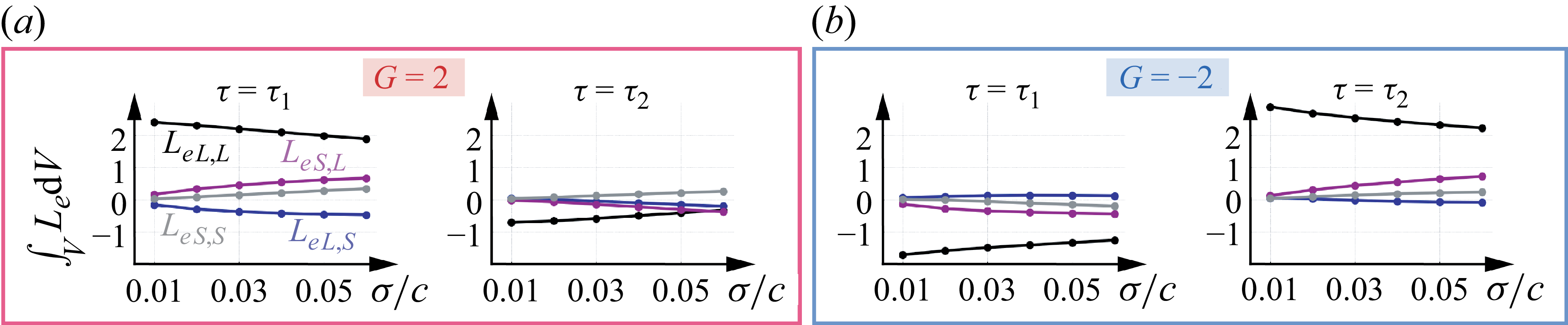
Let us also note that the extracted large-scale vortical structures at ${\textit{Re}}=$ 10 000 are primarily responsible for the significant lift peaks during the gust encounters. In figure 6, we present the volume integral of each term in (3.6) at $\tau =\tau _1$ and $\tau _2$ for $G=2$ and $-2$ with varying $\sigma /c$ . Here, the lift contribution from ${L_e}_{L,L}$ accounts for the majority of the lift peak values at $\tau =\tau _1$ and $\tau _2$ for both $G=2$ and $-2$ . Note that, for the minimum lift peaks at $\tau =\tau _2$ for $G=2$ and at $\tau =\tau _1$ for $G=-2$ , the total lift values are negative, to which ${L_e}_{L,L}$ contributes the most. This means that the extracted large-scale structures are the main contributors to the significant lift changes during the extreme gust encounters in the turbulent flow.

Figure 6. Volume integral of ${L_e}_{L,L}$ , ${L_e}_{S,L}$ , ${L_e}_{L,S}$ and ${L_e}_{S,S}$ at $\tau =\tau _1$ and $\tau _2$ over $\sigma /c$ for (a) $G=2$ and (b) $G=-2$ at ${\textit{Re}}=$ 10 000.

As $\sigma$ increases, a wider range of scales is incorporated as ‘small-scale’ structures, while the coverage of ‘large-scale’ structures decreases. Consequently, as $\sigma$ increases, the contribution of ${L_e}_{L,L}$ decreases, while that of ${L_e}_{S,S}$ increases, as seen for both gust ratios at $\tau =\tau _1$ and $\tau _2$ in figure 6. Furthermore, the contribution of ${L_e}_{S,L}$ rises as $\sigma$ increases. This term holds components based on the spatially compact vorticity field with spatially non-compact velocity field. With increased value of $\widetilde {\boldsymbol{\omega }}_{S}$ for a larger $\sigma$ , the contribution of ${L_e}_{S,L}$ increases slowly, even with more components being smoothed out for $\widetilde {\boldsymbol{u}}_{L}$ . For instance, at $\tau =\tau _2$ for the $G=2$ case (figure 6 a), while ${L_e}_{L,L}$ remains the largest contributor among the four terms for $\sigma /c \lesssim 0.05$ , ${L_e}_{S,L}$ becomes the most dominant past $\sigma /c \approx 0.06$ . In contrast, the contribution of ${L_e}_{L,S}$ does not grow as much with $\sigma$ . The larger $\sigma$ is, the less local motion of the fluid is contained in $\widetilde {\boldsymbol{u}}_{L}$ , causing $\widetilde {\boldsymbol{\omega }}_{L}$ to decrease significantly. Physically speaking, there cannot be a non-compact vorticity field producing a compact velocity field. As a result, the lift contribution of ${L_e}_{L,S}$ remains low.

Based on the observation of ${L_e}_{L,L}$ being the most responsible for the lift peaks at $\sigma /c \lesssim 0.05$ with both gust ratios, we have visualised the flowfield evaluated on $\widetilde {\boldsymbol{u}}_{L}$ with $\sigma /c=0.05$ in figures 2, 3 and 5. These findings show that the large-scale vortical structures in extreme gust encounters in turbulent regimes of at least $\sim \mathcal{O}(10^4)$ are not only similar to those observed in the laminar regimes, but also primarily responsible for the substantial transient lift changes, suggesting that studies in extreme aerodynamics at low Reynolds numbers can provide critical insights into those at higher Reynolds numbers.

Next, to mathematically quantify the similarity between these large-scale structures, we assess the similarity in the velocity field between the flows at ${\textit{Re}}=600$ and 10 000. Here, we use the cosine similarity in $L^2$ between velocity fields $\boldsymbol{u}_A$ and $\boldsymbol{u}_B$ defined as

(3.7) \begin{equation} S_c(\boldsymbol{u}_A,\boldsymbol{u}_B) = \frac {\int _V\boldsymbol{u}_A \boldsymbol{\cdot }\boldsymbol{u}_B\, {\rm d}V}{({\int _V||\boldsymbol{u}_A||^2\,{\rm d}V})^{1/2} ({\int _V||\boldsymbol{u}_B||^2\,{\rm d}V})^{1/2}}. \end{equation}

In this study, $V=[0,3]\times [-1,1]\times [-0.8,0.8]$ and we set $\boldsymbol{u}_A=\boldsymbol{u}-\boldsymbol{u_\infty }$ in the ${\textit{Re}}=600$ flow. We present the time history of $S_c(\boldsymbol{u}_A,\boldsymbol{u}_B)$ in figure 7 with $\boldsymbol{u}_B={\boldsymbol{u}}-\boldsymbol{u_\infty }$ , $\boldsymbol{u}_B=\widetilde {\boldsymbol{u}}_{L}-\boldsymbol{u_\infty }$ and $\boldsymbol{u}_B=\widetilde {\boldsymbol{u}}_{S}$ for the ${\textit{Re}}=$ 10 000 flow with $\sigma /c=0.05$ when filtering is considered.

Figure 7. Time history of $S_c$ for (a) $G=2$ and (b) $G=-2$ . The Q-criterion isosurface of the ${\textit{Re}}=600$ case (grey) and extracted large-scale structures of the ${\textit{Re}}=$ 10 000 case with $\sigma /c=0.05$ (green) at $\tau =\tau _3$ are visualised on the right of each panel.

High level of quantitative similarity $S_c$ of the ${\textit{Re}}=$ 10 000 case to the ${\textit{Re}}=600$ case is presented for both $G=2$ and $-2$ in figure 7. As shown, the similarity is attributed to the large-scale structures in the ${\textit{Re}}=$ 10 000 flow, and not the small-scale structures. Here, $S_c$ with $\boldsymbol{u}_B={\boldsymbol{u}}-\boldsymbol{u_\infty }$ or $\boldsymbol{u}_B=\widetilde {\boldsymbol{u}}_{L}-\boldsymbol{u_\infty }$ rises towards approximately $\tau =0$ . This is due to an increasing level of shared large-scale topological features, e.g. LEV, towards the initial interaction, where the incoming gust vortex mainly interacts with the leading edge of the wing. Past $\tau \approx 0$ , we notice that $S_c$ with $\boldsymbol{u}_B={\boldsymbol{u}}-\boldsymbol{u_\infty }$ and $\boldsymbol{u}_B=\widetilde {\boldsymbol{u}}_{L}-\boldsymbol{u_\infty }$ begin to decrease. This is caused by the differences in the evolution of the large-scale structures at different Reynolds numbers, as shown on the right of each panel in figure 7 that visualises the Q-criterion isosurface at ${\textit{Re}}=600$ and 10 000 (for $\sigma /c=0.05$ ) at $\tau =\tau _3$ . For instance, in the case with $G=2$ (figure 7 a), the TEV is located further downstream at $\tau =\tau _3$ for the ${\textit{Re}}=$ 10 000 case compared with that for ${\textit{Re}}=600$ . Nevertheless, the quantitative similarity remains high with $S_c$ above 0.6 even at $\tau =2$ . The resemblance of the large-scale structures identified at higher Reynolds numbers to those observed at lower Reynolds numbers underscores the importance of laminar flow analysis for deepening our fundamental understanding of the dominant dynamics in extreme aerodynamic flows. We note that the cosine similarity is a strict measure, since even the slightest difference in vortex position can significantly reduce the similarity. Other approaches such as the optimal transport analysis (Tran, Yeh & Taira Reference Tran, Yeh and Taira2026) can also be considered for convective physics highlighting similarities in a more generalised manner.