


1. Introduction
Non-spherical particles that interact through purely repulsive forces have been used for a long time as the simplest model of liquid crystals (Onsager Reference Onsager1949; De Gennes & Prost Reference De Gennes and Prost1993). Continuum theories of nematic liquid crystals describe the local orientation of particles through either a unit vector (Ericksen Reference Ericksen1961; Leslie Reference Leslie1968), called the director, or a tensor field, commonly known as the $\unicode{x1D64C}$
-tensor (De Gennes & Prost Reference De Gennes and Prost1993; Mottram & Newton Reference Mottram and Newton2014). The advantage of the
$\unicode{x1D64C}$
-tensor (De Gennes & Prost Reference De Gennes and Prost1993; Mottram & Newton Reference Mottram and Newton2014). The advantage of the $\unicode{x1D64C}$
-tensor formalism is that it can naturally deal with various levels of alignment and the possibility of orientation with two preferred directions (biaxial alignment, Mottram & Newton Reference Mottram and Newton2014). In both cases, an evolution equation for the orientation must be provided and coupled to the momentum and perhaps the mass balances to obtain a full set of differential equations to reproduce the dynamics of liquid crystals (Jenkins Reference Jenkins1978; Xu Reference Xu2022).
$\unicode{x1D64C}$
-tensor formalism is that it can naturally deal with various levels of alignment and the possibility of orientation with two preferred directions (biaxial alignment, Mottram & Newton Reference Mottram and Newton2014). In both cases, an evolution equation for the orientation must be provided and coupled to the momentum and perhaps the mass balances to obtain a full set of differential equations to reproduce the dynamics of liquid crystals (Jenkins Reference Jenkins1978; Xu Reference Xu2022).
In the last 15 years, there has been a growing interest in the granular physics community towards the collective behaviour of non-spherical grains, both through experiments and discrete element (DEM) numerical simulations (Börzsönyi et al. Reference Börzsönyi, Szabó, Törös, Wegner, Török, Somfai, Bien and Stannarius2012a , Reference Börzsönyi, Szabó, Wegner, Harth, Török, Somfai, Bien and Stannariusb ; Guo et al. Reference Guo, Wassgren, Ketterhagen, Hancock, James and Curtis2012; Wegner et al. Reference Wegner, Börzsönyi, Bien, Rose and Stannarius2012; Guo et al. Reference Guo, Wassgren, Hancock, Ketterhagen and Curtis2013; Szabó et al. Reference Szabó, Török, Somfai, Wegner, Stannarius, Böse, Rose, Angenstein and Börzsönyi2014; Guo & Curtis Reference Guo and Curtis2015; Buettner, Guo & Curtis Reference Buettner, Guo and Curtis2017; Harth et al. Reference Harth, Trittel, Wegner and Stannarius2018; Hidalgo et al. Reference Hidalgo, Szabó, Gillemot, Börzsönyi and Weinhart2018; Yang et al. Reference Yang, Guo, Buettner and Curtis2019; Pol et al. Reference Pol, Artoni, Richard, Nunes Da Conceição and Gabrieli2022, Reference Pol, Artoni and Richard2023). The interest stems from the vast amount of industrial applications of non-spherical particulates, and also from the progress in DEM simulations, that nowadays permits the simulation of thousands of particles in non-trivial geometries at a reasonable computational cost.
In the context of granular physics, attempts have been made to phenomenologically incorporate particle orientation in the rheological response, using both inertial rheology (Nagy et al. Reference Nagy, Claudin, Börzsönyi and Somfai2017, Reference Nagy, Claudin, Börzsönyi and Somfai2020) and kinetic theory of granular gases (Berzi et al. Reference Berzi, Thai-Quang, Guo and Curtis2016, Reference Berzi, Thai-Quang, Guo and Curtis2017, Reference Berzi, Buettner and Curtis2022). Inertial rheology (MiDi Reference MiDi2004) ignores the role of particle agitation, which is instead the main ingredient in the kinetic theory of granular gases (Jenkins & Savage Reference Jenkins and Savage1983; Lun Reference Lun1991; Garzó & Dufty Reference Garzó and Dufty1999). Recently, inertial rheology has been shown to be a special case of kinetic theory (Berzi Reference Berzi2024).
A further improvement has been achieved by describing the alignment through an orientational tensor, de facto the $\unicode{x1D64C}$
-tensor of liquid crystals, although no connection was explicitly established. An evolution equation for the tensor has been expressed and coupled with inertial rheology (Nadler, Guillard & Einav Reference Nadler, Guillard and Einav2018; Nadler Reference Nadler2021) or kinetic theory (Vescovi et al. Reference Vescovi, Nadler and Berzi2024b
) to describe orientation and stresses in steady and homogeneous shear flows of ellipsoids and cylinders. The possibility of diffusion of orientation originating from the interaction between a shear flow of uniaxial grains and solid boundaries has also been incorporated (Amereh & Nadler Reference Amereh and Nadler2022).
$\unicode{x1D64C}$
-tensor of liquid crystals, although no connection was explicitly established. An evolution equation for the tensor has been expressed and coupled with inertial rheology (Nadler, Guillard & Einav Reference Nadler, Guillard and Einav2018; Nadler Reference Nadler2021) or kinetic theory (Vescovi et al. Reference Vescovi, Nadler and Berzi2024b
) to describe orientation and stresses in steady and homogeneous shear flows of ellipsoids and cylinders. The possibility of diffusion of orientation originating from the interaction between a shear flow of uniaxial grains and solid boundaries has also been incorporated (Amereh & Nadler Reference Amereh and Nadler2022).
In this paper, we will attempt to unify the $\unicode{x1D64C}$
-tensor theory of liquid crystals and the kinetic theory of granular gases. We will phrase and solve a system of differential equations, with appropriate boundary conditions, governing the velocity fluctuations and the orientation, under steady conditions and in the absence of gravity and shearing, of both rod-like and disk-like grains. The particles are contained in a quasi-2D square box within two vibrating and two non-vibrating flat walls. We will show that the agitation injected through the wall vibration causes inhomogeneities in the density of the system, which in turn induces gradients in the orientational tensor and permits the transition from an isotropic (random alignment) to a nematic (preferential alignment) phase to take place inside the domain. We will also show that the theory can qualitatively and quantitatively reproduce the fields of velocity fluctuations and elements of the orientational tensor against DEM simulations performed with ellipsoids of different length-to-diameter ratio.
$\unicode{x1D64C}$
-tensor theory of liquid crystals and the kinetic theory of granular gases. We will phrase and solve a system of differential equations, with appropriate boundary conditions, governing the velocity fluctuations and the orientation, under steady conditions and in the absence of gravity and shearing, of both rod-like and disk-like grains. The particles are contained in a quasi-2D square box within two vibrating and two non-vibrating flat walls. We will show that the agitation injected through the wall vibration causes inhomogeneities in the density of the system, which in turn induces gradients in the orientational tensor and permits the transition from an isotropic (random alignment) to a nematic (preferential alignment) phase to take place inside the domain. We will also show that the theory can qualitatively and quantitatively reproduce the fields of velocity fluctuations and elements of the orientational tensor against DEM simulations performed with ellipsoids of different length-to-diameter ratio.
2. Theory and simulations
We consider uniaxial particles of mass density $\rho _p$
that can be characterised by two dimensions, axial length,
$\rho _p$
that can be characterised by two dimensions, axial length, $l$
, and transverse size,
$l$
, and transverse size, $d$
. The grains can be represented by the equivalent diameter
$d$
. The grains can be represented by the equivalent diameter $d_v$
of a sphere of equal volume (e.g.
$d_v$
of a sphere of equal volume (e.g. $d_v= ((3/2)d^2l )^{1/3}$
in the case of cylinders and
$d_v= ((3/2)d^2l )^{1/3}$
in the case of cylinders and $d_v= (d^2l )^{1/3}$
in the case of ellipsoids), and their aspect ratio, which we measure through the shape factor
$d_v= (d^2l )^{1/3}$
in the case of ellipsoids), and their aspect ratio, which we measure through the shape factor $r_g=(l-d)/(l+d)$
, with
$r_g=(l-d)/(l+d)$
, with $0\lt r_g\lt 1$
for
$0\lt r_g\lt 1$
for $l/d\gt 1$
(prolate particles) and
$l/d\gt 1$
(prolate particles) and $-1\lt r_g\lt 0$
for
$-1\lt r_g\lt 0$
for $l/d\lt 1$
(oblate particles). The volume of the particles over the total volume is the solid volume fraction,
$l/d\lt 1$
(oblate particles). The volume of the particles over the total volume is the solid volume fraction, $\nu$
, and we characterise their agitation through the granular temperature
$\nu$
, and we characterise their agitation through the granular temperature $T$
, one-third of the mean square of the particle velocity fluctuations.
$T$
, one-third of the mean square of the particle velocity fluctuations.
2.1. $\unicode{x1D64C}$
-tensor theory
$\unicode{x1D64C}$
-tensor theory

The orientation of a particle $i$
is defined by the dyad
$i$
is defined by the dyad $({\boldsymbol{k}}{_i}\otimes {\boldsymbol{k}}{_i})$
, where
$({\boldsymbol{k}}{_i}\otimes {\boldsymbol{k}}{_i})$
, where ${\boldsymbol{k}}{_i}$
is a unit vector aligned with the grain symmetry axis. For an assembly of
${\boldsymbol{k}}{_i}$
is a unit vector aligned with the grain symmetry axis. For an assembly of $N$
particles, orientation is defined by the traceless, symmetric tensor
$N$
particles, orientation is defined by the traceless, symmetric tensor
 \begin{equation} {\unicode{x1D64C}} = \frac {1}{N}\sum _{i=1}^N \left ( {\boldsymbol{k}}_i \otimes {\boldsymbol{k}}_i\right )-\dfrac {1}{3}\unicode{x1D644}, \end{equation}
where $\unicode{x1D644}$
is the identity matrix. This tensor was first introduced in the context of liquid crystals (Mottram & Newton Reference Mottram and Newton2014; Liu & Wang Reference Liu and Wang2016), and has all eigenvalues in
$\unicode{x1D644}$
is the identity matrix. This tensor was first introduced in the context of liquid crystals (Mottram & Newton Reference Mottram and Newton2014; Liu & Wang Reference Liu and Wang2016), and has all eigenvalues in $[-1/3,2/3]$
.
$[-1/3,2/3]$
.
The orientational tensor is assumed to be governed by a balance law of the form (Xu Reference Xu2022)
 \begin{equation} \dot {{\unicode{x1D64C}}} = \unicode{x1D64E} +\varGamma {\unicode{x1D643}}, \end{equation}
where $\dot {{\unicode{x1D64C}}}$
is the material time derivative of the orientational tensor,
$\dot {{\unicode{x1D64C}}}$
is the material time derivative of the orientational tensor, $\unicode{x1D64E}$
accounts for the co-rotation and stretching effect of the flow and
$\unicode{x1D64E}$
accounts for the co-rotation and stretching effect of the flow and $\unicode{x1D643}$
, proportional to
$\unicode{x1D643}$
, proportional to $\rho _p\nu T$
, is responsible for the relaxation to the minimum of the free energy density. The coefficient
$\rho _p\nu T$
, is responsible for the relaxation to the minimum of the free energy density. The coefficient $\varGamma$
, which is proportional to
$\varGamma$
, which is proportional to $1/ (\rho _p\nu T^{1/2} d_v )$
, represents rotational diffusion and is actually the inverse of a rotational viscosity (Mottram & Newton Reference Mottram and Newton2014; Liu & Wang Reference Liu and Wang2016).
$1/ (\rho _p\nu T^{1/2} d_v )$
, represents rotational diffusion and is actually the inverse of a rotational viscosity (Mottram & Newton Reference Mottram and Newton2014; Liu & Wang Reference Liu and Wang2016).
The expression for $\unicode{x1D64E}$
in the liquid crystal literature (Xu Reference Xu2022), which was also formulated in Vescovi et al. (Reference Vescovi, Nadler and Berzi2024b
) for steady-state homogeneous shear flows of cylinders, reads
$\unicode{x1D64E}$
in the liquid crystal literature (Xu Reference Xu2022), which was also formulated in Vescovi et al. (Reference Vescovi, Nadler and Berzi2024b
) for steady-state homogeneous shear flows of cylinders, reads
 \begin{equation} \unicode{x1D64E} = \left ({\boldsymbol{\varOmega }}+ \phi {\unicode{x1D63F}}\right )\left ({\unicode{x1D64C}}+\dfrac {1}{3}\unicode{x1D644}\right ) -\left ({\unicode{x1D64C}}+\dfrac {1}{3}\unicode{x1D644}\right )\left ({\boldsymbol{\varOmega }}-\phi {\unicode{x1D63F}}\right ) - 2\phi \left ( {\unicode{x1D64C}} : {\unicode{x1D63F}} \right ) \left ({\unicode{x1D64C}}+\dfrac {1}{3}\unicode{x1D644}\right )\!, \end{equation}
where ${\boldsymbol{\varOmega }}=(\boldsymbol{\nabla }{\boldsymbol{v}} - \boldsymbol{\nabla }{\boldsymbol{v}}^{\textrm{T}})/2$
is the spin tensor,
${\boldsymbol{\varOmega }}=(\boldsymbol{\nabla }{\boldsymbol{v}} - \boldsymbol{\nabla }{\boldsymbol{v}}^{\textrm{T}})/2$
is the spin tensor, ${\unicode{x1D63F}}=(\boldsymbol{\nabla }{\boldsymbol{v}} + \boldsymbol{\nabla }{\boldsymbol{v}}^{\textrm{T}})/2$
is the deformation rate of the velocity field
${\unicode{x1D63F}}=(\boldsymbol{\nabla }{\boldsymbol{v}} + \boldsymbol{\nabla }{\boldsymbol{v}}^{\textrm{T}})/2$
is the deformation rate of the velocity field $\boldsymbol{v}$
, and the flow alignment parameter
$\boldsymbol{v}$
, and the flow alignment parameter $\phi$
was determined by fitting to discrete simulations (Vescovi et al. Reference Vescovi, Nadler and Berzi2024b
).
$\phi$
was determined by fitting to discrete simulations (Vescovi et al. Reference Vescovi, Nadler and Berzi2024b
).
The usual assumption is that the free energy density, $\mathcal{F}$
, of the particles is (Mottram & Newton Reference Mottram and Newton2014)
$\mathcal{F}$
, of the particles is (Mottram & Newton Reference Mottram and Newton2014)
 \begin{equation} \mathcal{F} = \dfrac {a}{2}{\textrm{tr}} ({\unicode{x1D64C}\,}^2)-\dfrac {b}{3}{\textrm{tr}} ({\unicode{x1D64C}\,}^3)+\dfrac {c}{4}{\textrm{tr}}^2\big ({\unicode{x1D64C}}^2\big )+\dfrac {L}{2}\big \lvert \boldsymbol{\nabla }{\unicode{x1D64C}}\big \rvert ^2. \end{equation}
The first three terms, which contain the coefficients $a$
,
$a$
, $b$
and
$b$
and $c$
, represent the Landau–de Gennes form for the bulk free energy density (Mottram & Newton Reference Mottram and Newton2014, a fourth-order degree polynomial). They ensure that
$c$
, represent the Landau–de Gennes form for the bulk free energy density (Mottram & Newton Reference Mottram and Newton2014, a fourth-order degree polynomial). They ensure that $\mathcal{F}$
has two minima: one is
$\mathcal{F}$
has two minima: one is
![]() , the isotropic state; and one is
, the isotropic state; and one is
![]() , the nematic state. The last term on the right-hand side of (2.4) instead represents the (entropic) elastic component of the free energy density and is introduced to penalise the distortion of the alignment. Here,
, the nematic state. The last term on the right-hand side of (2.4) instead represents the (entropic) elastic component of the free energy density and is introduced to penalise the distortion of the alignment. Here, $L$
is the Frank coefficient in the one-constant approximation of the Oseen–Frank (entropic) elastic energy (Heymans & Schilling Reference Heymans and Schilling2017).
$L$
is the Frank coefficient in the one-constant approximation of the Oseen–Frank (entropic) elastic energy (Heymans & Schilling Reference Heymans and Schilling2017).
The variational principle implies that ${\unicode{x1D643}}=-\partial \mathcal{F}/\partial {\unicode{x1D64C}}+\boldsymbol{\nabla }\boldsymbol{\cdot } (\partial \mathcal{F}/\partial \boldsymbol{\nabla \!}{\unicode{x1D64C}} )$
is the term responsible for driving
${\unicode{x1D643}}=-\partial \mathcal{F}/\partial {\unicode{x1D64C}}+\boldsymbol{\nabla }\boldsymbol{\cdot } (\partial \mathcal{F}/\partial \boldsymbol{\nabla \!}{\unicode{x1D64C}} )$
is the term responsible for driving $\unicode{x1D64C}$
to equilibrium. From (2.4),
$\unicode{x1D64C}$
to equilibrium. From (2.4),
 \begin{equation} \dfrac {{\unicode{x1D643}}}{\rho _p\nu T} = - \tilde {a} {\unicode{x1D64C}}+\tilde {b}\left [{\unicode{x1D64C}}^2-\dfrac {1}{3}{\textrm{tr}} ({\unicode{x1D64C}\,}^2)\unicode{x1D644}\right ]- \tilde {c}{\unicode{x1D64C}}\, {\textrm{tr}} ({\unicode{x1D64C}\,}^2 )+\dfrac {1}{ T}\boldsymbol{\nabla }\boldsymbol{\cdot }\big ( \tilde Ld_v^2 T \boldsymbol{\nabla }{\unicode{x1D64C}}\big ). \end{equation}
The parameters $\tilde a$
,
$\tilde a$
, $\tilde b$
and
$\tilde b$
and $\tilde c$
are the dimensionless form of the corresponding parameters
$\tilde c$
are the dimensionless form of the corresponding parameters $a$
,
$a$
, $b$
and
$b$
and $c$
in the bulk free energy. The parameter
$c$
in the bulk free energy. The parameter $\tilde L=L/ ( \rho _p\nu T d_v^2 )$
is the dimensionless form of the Frank elastic coefficient and depends on the shape factor. Unlike the common assumption of the Beris–Edwards model (Xu Reference Xu2022) that
$\tilde L=L/ ( \rho _p\nu T d_v^2 )$
is the dimensionless form of the Frank elastic coefficient and depends on the shape factor. Unlike the common assumption of the Beris–Edwards model (Xu Reference Xu2022) that $L$
is spatially homogeneous, here we account for the possible spatial variations of at least the temperature in the expression for
$L$
is spatially homogeneous, here we account for the possible spatial variations of at least the temperature in the expression for $L$
, and write the elastic term as the divergence of a flux of
$L$
, and write the elastic term as the divergence of a flux of $\unicode{x1D64C}$
.
$\unicode{x1D64C}$
.
In the case of liquid crystals composed of hard particles, $\tilde b$
and
$\tilde b$
and $\tilde c$
are positive functions of the shape factor and independent of the solid volume fraction. On the other hand,
$\tilde c$
are positive functions of the shape factor and independent of the solid volume fraction. On the other hand, $\tilde a=\tilde \alpha (\nu ^*-\nu )$
, where
$\tilde a=\tilde \alpha (\nu ^*-\nu )$
, where $\tilde \alpha \gt 0$
depends on the shape factor and
$\tilde \alpha \gt 0$
depends on the shape factor and $\nu ^*$
is the specific volume fraction at which
$\nu ^*$
is the specific volume fraction at which $\tilde a$
changes sign (a necessary condition for the isotropic–nematic transition to take place (Mottram & Newton Reference Mottram and Newton2014). Given that the difference between
$\tilde a$
changes sign (a necessary condition for the isotropic–nematic transition to take place (Mottram & Newton Reference Mottram and Newton2014). Given that the difference between $\nu ^*$
and the volume fraction at which the isotropic–nematic transition actually takes place is small (Mottram & Newton Reference Mottram and Newton2014), we can confuse
$\nu ^*$
and the volume fraction at which the isotropic–nematic transition actually takes place is small (Mottram & Newton Reference Mottram and Newton2014), we can confuse $\nu ^*$
with the latter and fit the data obtained in Monte Carlo simulations of hard ellipsoids (Odriozola Reference Odriozola2012) with the following function of the shape factor (see Appendix A):
$\nu ^*$
with the latter and fit the data obtained in Monte Carlo simulations of hard ellipsoids (Odriozola Reference Odriozola2012) with the following function of the shape factor (see Appendix A):
 \begin{equation} \nu ^* \approx -0.77r_g^2+0.04r_g+0.71. \end{equation}
2.2. DEM simulations and kinetic theory
We have performed DEM simulations, using MercuryDPM (www.mercurydpm.org, Weinhart et al. Reference Weinhart2019), of a densely packed assembly of $N$
identical frictionless ellipsoids of mass density
$N$
identical frictionless ellipsoids of mass density $\rho _p$
and restitution coefficient
$\rho _p$
and restitution coefficient $e_n=0.95$
(the negative of the ratio of post- to pre-collisional relative velocity normal to the plane of contact). Particles interact through linear spring-dashpots. More details about the contact force model are provided in Appendix B. The ellipsoids are contained in a box cell with four solid flat frictionless walls, in the absence of gravity. Two parallel walls perpendicular to the
$e_n=0.95$
(the negative of the ratio of post- to pre-collisional relative velocity normal to the plane of contact). Particles interact through linear spring-dashpots. More details about the contact force model are provided in Appendix B. The ellipsoids are contained in a box cell with four solid flat frictionless walls, in the absence of gravity. Two parallel walls perpendicular to the $y$
-direction vibrate with constant amplitude
$y$
-direction vibrate with constant amplitude $\lambda =0.1d_v$
and constant angular frequency
$\lambda =0.1d_v$
and constant angular frequency $\omega$
, while the other two parallel walls perpendicular to the
$\omega$
, while the other two parallel walls perpendicular to the $x$
-direction do not move. Periodic boundary conditions are used in the
$x$
-direction do not move. Periodic boundary conditions are used in the $z$
-direction. The dimensions of the box along the three directions are
$z$
-direction. The dimensions of the box along the three directions are $l_x=l_y=10 d_v$
and
$l_x=l_y=10 d_v$
and $l_z=5 d_v$
.
$l_z=5 d_v$
.
We initially placed the ellipsoids at random in the box and let the system evolve. Unless otherwise stated, the average solid volume fraction is $\bar \nu = N\pi d_v^3/ (6l_xl_yl_z )=0.4$
. With this, we anticipate that the local solid volume fraction is in the range 0.28–0.58 everywhere in the box cell, well below the critical value at which we expect the presence of rate-independent components of stresses (Berzi, Buettner & Curtis Reference Berzi, Buettner and Curtis2022) and below the value at which ellipsoids such as those employed in the present simulations experience a nematic–smectic transition (Odriozola Reference Odriozola2012). In this condition, the only velocity scale of the system is
$\bar \nu = N\pi d_v^3/ (6l_xl_yl_z )=0.4$
. With this, we anticipate that the local solid volume fraction is in the range 0.28–0.58 everywhere in the box cell, well below the critical value at which we expect the presence of rate-independent components of stresses (Berzi, Buettner & Curtis Reference Berzi, Buettner and Curtis2022) and below the value at which ellipsoids such as those employed in the present simulations experience a nematic–smectic transition (Odriozola Reference Odriozola2012). In this condition, the only velocity scale of the system is $\lambda \omega$
. Hence, without loss of generality, we have set
$\lambda \omega$
. Hence, without loss of generality, we have set $\rho _p$
,
$\rho _p$
, $d_v$
and
$d_v$
and $\lambda \omega$
equal to one in the simulations.
$\lambda \omega$
equal to one in the simulations.
If the system reaches a steady state with zero mean velocity, ![]() and the balance of orientation (2.2) takes the simple form
and the balance of orientation (2.2) takes the simple form
 \begin{equation} -\boldsymbol{\nabla }\boldsymbol{\cdot }\big (-\tilde {L}d_v^2T\boldsymbol{\nabla }{\unicode{x1D64C}}\big ) = T \left \{\tilde {a} {\unicode{x1D64C}}-\tilde {b}\left [{\unicode{x1D64C}}^2-\dfrac {1}{3}{\textrm{tr}} ({\unicode{x1D64C}\,}^2)\unicode{x1D644}\right ]+ \tilde {c}{\unicode{x1D64C}}\, {\textrm{tr}} ({\unicode{x1D64C}\,}^2 )\right \}\!. \end{equation}
The left-hand side of (2.7) is the negative of the divergence of the orientational flux.
Similarly, the granular temperature is governed by the balance of kinetic energy associated with the fluctuations in translational velocity (Garzó & Dufty Reference Garzó and Dufty1999), which, in the absence of shearing and in the steady state, reduces to a balance between the diffusion of energy and its dissipation via inelastic collisions:
 \begin{equation} -\!\boldsymbol{\nabla }\boldsymbol{\cdot } \big (- {\unicode{x1D646}}\, \boldsymbol{\nabla }T\big ) = \dfrac {6\big (1-e_n\big )p}{\pi ^{1/2}d_v}f\big (r_g\big )T^{1/2}, \end{equation}
where $p$
is the pressure. The left-hand side of (2.8) is the negative of the divergence of the fluctuation energy flux, in which
$p$
is the pressure. The left-hand side of (2.8) is the negative of the divergence of the fluctuation energy flux, in which $\unicode{x1D646}$
is the diffusivity tensor. The right-hand side of (2.8) is the rate of collisional dissipation and includes a function of the shape factor,
$\unicode{x1D646}$
is the diffusivity tensor. The right-hand side of (2.8) is the rate of collisional dissipation and includes a function of the shape factor, $f (r_g )$
, that modifies the classical expression for spherical grains to account for the additional dissipation induced by particle rotation. An explicit expression,
$f (r_g )$
, that modifies the classical expression for spherical grains to account for the additional dissipation induced by particle rotation. An explicit expression,
 \begin{equation} f\big (r_g\big )=\left (0.65\dfrac {1+\lvert r_g\rvert }{1-\lvert r_g\rvert }+1.39\right ) \end{equation}
has been proposed in the case of elongated cylinders by Buettner et al. (Reference Buettner, Guo and Curtis2017). With respect to the expression proposed by Buettner et al. (Reference Buettner, Guo and Curtis2017), here we use the absolute value of the shape factor to deal with both prolate and oblate grains. Notice that we expect (2.9) to overestimate dissipation in the case of ellipsoids: cylinders have a larger excluded volume with respect to ellipsoids, leading to higher frequency of collisions and larger dissipation; also, the presence of sharp ends and flat sides should lead to more abrupt collisions in the case of cylinders, and a stronger coupling between rotational and translational motion. Also notice that modifications of the collisional dissipation rate to deal with frictional rather than frictionless particles are available (Buettner, Guo & Curtis Reference Buettner, Guo and Curtis2020).
In the case of spheres, the diffusivity is isotropic and $\unicode{x1D646}$
can be written as
$\unicode{x1D646}$
can be written as
 \begin{equation} {\unicode{x1D646}} = \dfrac {2M_\infty d_v p}{\pi ^{1/2}\left (1+e_n\right )T^{1/2}}\unicode{x1D644}. \end{equation}
Here, with respect to the expression derived by Garzó & Dufty (Reference Garzó and Dufty1999), we have made use of the fact that, in the dense limit, the dependence of the diffusivity on the solid volume fraction can be equivalently expressed as $p/ [2 (1+e_n )T ]$
, (Berzi Reference Berzi2024), and
$p/ [2 (1+e_n )T ]$
, (Berzi Reference Berzi2024), and
 \begin{equation} M_\infty = 4.5\left [\dfrac {1+e_n}{2}+\dfrac {9\pi }{8}\dfrac {\left (1+e_n\right )^3\left (2e_n-1\right )}{16\left (1+e_n\right )-7\left (1-e_n^2\right )}\right ]\!. \end{equation}
Note that we have introduced a prefactor equal to 4.5 with respect to the usual expression for $M_\infty$
, otherwise the diffusivity would be underestimated even in the case of spheres. This underestimation was already noticed in Vescovi et al. (Reference Vescovi, de Wijn, Cross and Berzi2024a
) in the case of steady, homogeneous shearing of frictionless spheres between bumpy walls.
$M_\infty$
, otherwise the diffusivity would be underestimated even in the case of spheres. This underestimation was already noticed in Vescovi et al. (Reference Vescovi, de Wijn, Cross and Berzi2024a
) in the case of steady, homogeneous shearing of frictionless spheres between bumpy walls.
In the case of uniaxial grains with some preferential orientation, the anisotropy implies that the fluctuation energy can diffuse more efficiently along some directions. Similarly to what we have done for the shear viscosity in the case of shearing flows of uniaxial grains (Vescovi et al. Reference Vescovi, Nadler and Berzi2024b ), we introduce a linear dependence of the diffusivity tensor on the orientational tensor,
 \begin{equation} {\unicode{x1D646}} = \dfrac {2M_\infty d_v p}{\pi ^{1/2}\left (1+e_n\right )T^{1/2}}\big (\unicode{x1D644}+\varphi {\unicode{x1D64C}}\big ). \end{equation}
The coefficient $\varphi$
must depend on the shape of the particle and the surface friction and accounts for the anisotropy in the thermal diffusivity between the direction parallel and perpendicular to the alignment. Previous experimental and theoretical work in the context of liquid crystals showed that the diffusivity is enhanced in the direction parallel (perpendicular) to the alignment for prolate (oblate) particles, i.e.
$\varphi$
must depend on the shape of the particle and the surface friction and accounts for the anisotropy in the thermal diffusivity between the direction parallel and perpendicular to the alignment. Previous experimental and theoretical work in the context of liquid crystals showed that the diffusivity is enhanced in the direction parallel (perpendicular) to the alignment for prolate (oblate) particles, i.e. $\varphi$
is positive (negative) (Simões et al. Reference Simões, Palangana, Steudel, Kimura and Gómez2008). It also showed that
$\varphi$
is positive (negative) (Simões et al. Reference Simões, Palangana, Steudel, Kimura and Gómez2008). It also showed that $\varphi$
should be of order unity.
$\varphi$
should be of order unity.
Assuming that the pressure $p$
in steady state is homogeneous, (2.7) and (2.8) simplify to
$p$
in steady state is homogeneous, (2.7) and (2.8) simplify to
 \begin{equation} \delta ^2 \boldsymbol{\nabla }\boldsymbol{\cdot } (T\boldsymbol{\nabla }{\unicode{x1D64C}})= T\left \{ (\nu ^*-\nu ) {\unicode{x1D64C}}-\dfrac {\tilde {b}}{\tilde {\alpha }}\left [{\unicode{x1D64C}\,}^2-\dfrac {1}{3}{\textrm{tr}} ({\unicode{x1D64C}\,}^2)\unicode{x1D644}\right ]+ \dfrac {\tilde {c}}{\tilde {\alpha }}{\unicode{x1D64C}}\, {\textrm{tr}} ({\unicode{x1D64C}\,}^2)\right \} \end{equation}
and
 \begin{equation} \epsilon ^2 \boldsymbol{\nabla }\boldsymbol{\cdot } \big [\big (\unicode{x1D644}+\varphi {\unicode{x1D64C}}\big )\boldsymbol{\nabla }T^{1/2}\big ] = T^{1/2}, \end{equation}
respectively, where $\delta = d_v (\tilde L/\tilde \alpha )^{1/2}$
and
$\delta = d_v (\tilde L/\tilde \alpha )^{1/2}$
and
 \begin{equation} \epsilon = d_v \left [\dfrac {2M_\infty }{3\big (1-e_n^2\big )f (r_g)}\right ]^{1/2} \end{equation}
are two characteristic lengths for the diffusion of orientation and velocity fluctuations.
In the context of liquid crystals, the Beris–Edwards model (Beris & Edwards Reference Beris and Edwards1994; Xu Reference Xu2022) assumes incompressibility and therefore treats the solid volume fraction $\nu$
in (2.13) as a constant. Here, we will show that allowing for variations in the solid volume fraction permits the reproduction of striking features of the numerical simulations, such as the isotropic–nematic transition taking place inside the domain, at some distance from the boundaries. To account for compressibility, we must introduce an equation of state.
$\nu$
in (2.13) as a constant. Here, we will show that allowing for variations in the solid volume fraction permits the reproduction of striking features of the numerical simulations, such as the isotropic–nematic transition taking place inside the domain, at some distance from the boundaries. To account for compressibility, we must introduce an equation of state.
Explicit expressions for the equation of state in the isotropic phase of hard convex bodies have been proposed in the literature (Vega, Lago & Garzon Reference Vega, Lago and Garzon1994; Vega Reference Vega1997), without including the role of the coefficient of restitution. Recently, it has been shown that the particle shape has only a small influence on the equation of state in DEM simulations of cylinders under simple shearing (Berzi et al. Reference Berzi, Thai-Quang, Guo and Curtis2016), and that the Carnahan & Starling (Reference Carnahan and Starling1969) expression,
 \begin{equation} p = \rho _p T \dfrac {\nu +\nu ^2+\nu ^3-\nu ^4}{\left (1-\nu \right )^3}, \end{equation}
is sufficiently accurate up to moderate volume fractions, at least if the coefficient of restitution is not too far from one. To facilitate the numerical integration of the differential equations, here we expand this expression around the average volume fraction $\bar \nu$
and express
$\bar \nu$
and express $\nu$
in (2.13) as
$\nu$
in (2.13) as
 \begin{equation} \nu =\bar \nu + \left [\dfrac {p}{\rho _p T } - \dfrac {\bar \nu +\bar \nu ^2+\bar \nu ^3-\bar \nu ^4}{\left (1-\bar \nu \right )^3}\right ]\dfrac {\left (1-\bar \nu \right )^4}{\bar \nu ^4-4\bar \nu ^3+4\bar \nu ^2+4\bar \nu +1}. \end{equation}
It is worth mentioning that the equation of state (2.16) is not valid in the nematic phase (Frenkel & Mulder Reference Frenkel and Mulder1985), but we claim that it is still sufficiently accurate if the solid volume fraction is not too far from the value at the isotropic–nematic transition.
2.3. Boundary conditions
For the granular temperature, the balance of fluctuation energy phrased at the boundary prescribes that the component of the fluctuation energy flux normal to the wall and directed inward must be equal to $I-D$
where
$I-D$
where $I\approx (\lambda \omega )^2 p/ T_w^{1/2}$
is the energy input from a vibrating wall (Soto Reference Soto2004), and
$I\approx (\lambda \omega )^2 p/ T_w^{1/2}$
is the energy input from a vibrating wall (Soto Reference Soto2004), and $D= (2/\pi )^{1/2} (1-e_w) p T_w^{1/2}$
is the energy dissipation from the impacts of particles on a wall (Richman Reference Richman1988; Jenkins Reference Jenkins2007), where
$D= (2/\pi )^{1/2} (1-e_w) p T_w^{1/2}$
is the energy dissipation from the impacts of particles on a wall (Richman Reference Richman1988; Jenkins Reference Jenkins2007), where $e_w$
is the coefficient of restitution between the wall and the particles. The subscript
$e_w$
is the coefficient of restitution between the wall and the particles. The subscript $w$
indicates quantities evaluated at the walls. Here we consider
$w$
indicates quantities evaluated at the walls. Here we consider $e_w = e_n = 0.95$
.
$e_w = e_n = 0.95$
.
With the flux of fluctuation energy given in (2.8), the boundary condition for the square root of the granular temperature at the walls is, then,
 \begin{equation} {\boldsymbol{n}}\boldsymbol{\cdot } \big [(\unicode{x1D644}+\varphi {\unicode{x1D64C}}) \boldsymbol{\nabla }T^{1/2}\big ] \big \rvert _w = \left [1 -\dfrac {\beta }{\zeta }\dfrac {(\lambda \omega )^2}{ T_w} \right ] \dfrac {T_w^{1/2}}{\beta }, \end{equation}
where $\boldsymbol{n}$
is the unit inward normal to the boundary. Here,
$\boldsymbol{n}$
is the unit inward normal to the boundary. Here,
 \begin{equation} \zeta = d_v \dfrac {4M_\infty } {\left (2\pi \right )^{1/2}\left (1+e_n\right )} \end{equation}
and
 \begin{equation} \beta = d_v \dfrac {4M_\infty } {2^{1/2}\left (1-e_w\right )\left (1+e_n\right )} \end{equation}
are two characteristic lengths associated with the energy input from vibrating walls and the energy dissipated in wall collisions, respectively. The factor $2^{1/2}$
in the denominator of (2.19) allows us to better fit the results of discrete simulations in the case of spheres.
$2^{1/2}$
in the denominator of (2.19) allows us to better fit the results of discrete simulations in the case of spheres.
For the boundary condition on the orientation, we adopt the usual assumption that the normal inward flux of $\unicode{x1D64C}$
at the boundary is proportional to the jump in
$\unicode{x1D64C}$
at the boundary is proportional to the jump in $\unicode{x1D64C}$
there. This is known as weak anchoring in the context of liquid crystals (Mottram & Newton Reference Mottram and Newton2014). Then, with the flux of orientation given in (2.7),
$\unicode{x1D64C}$
there. This is known as weak anchoring in the context of liquid crystals (Mottram & Newton Reference Mottram and Newton2014). Then, with the flux of orientation given in (2.7),
 \begin{equation} {\boldsymbol{n}}\boldsymbol{\cdot }\big ( \tilde L d_v^2T\boldsymbol{\nabla }{\unicode{x1D64C}}\big )\big \rvert _w = \dfrac {W}{\rho _p\nu _w } [\![\! {\unicode{x1D64C}} ]\!]_w , \end{equation}
where $[\![\! {\unicode{x1D64C}} ]\!]_w = {\unicode{x1D64C}}_w - {\unicode{x1D64C}}_b$
is the jump in the orientational tensor at the boundary,
$[\![\! {\unicode{x1D64C}} ]\!]_w = {\unicode{x1D64C}}_w - {\unicode{x1D64C}}_b$
is the jump in the orientational tensor at the boundary, ${\unicode{x1D64C}}_b$
is the preferred orientation at the boundary, and
${\unicode{x1D64C}}_b$
is the preferred orientation at the boundary, and $W$
is the anchoring strength (Mottram & Newton Reference Mottram and Newton2014). Here, we assume that
$W$
is the anchoring strength (Mottram & Newton Reference Mottram and Newton2014). Here, we assume that
 \begin{equation} W = \rho _p\nu T_w\dfrac {T_w}{\left (\lambda \omega \right )^2}\tilde W d_v, \end{equation}
that is, the anchoring strength is an Onsager-like term due to loss of entropy near the wall (proportional to $\rho _p\nu _w T_w d_v$
, Poniewierski & Hoiyst Reference Poniewierski and Hoiyst1988) dynamically weakened in case of wall vibration (the correction is the ratio of
$\rho _p\nu _w T_w d_v$
, Poniewierski & Hoiyst Reference Poniewierski and Hoiyst1988) dynamically weakened in case of wall vibration (the correction is the ratio of $\rho _p\nu T_w$
over the average kinetic energy of particles moving with the wall,
$\rho _p\nu T_w$
over the average kinetic energy of particles moving with the wall, $\rho _p\nu (\lambda \omega )^2$
). The dimensionless coefficient
$\rho _p\nu (\lambda \omega )^2$
). The dimensionless coefficient $\tilde W$
is a function of the particle shape. Then, (2.21) becomes
$\tilde W$
is a function of the particle shape. Then, (2.21) becomes
 \begin{equation} {\boldsymbol{n}}\boldsymbol{\cdot } \big (T\boldsymbol{\nabla }{\unicode{x1D64C}}\big )\big \rvert _w = \dfrac {T_w^2}{\left (\lambda \omega \right )^2}\dfrac {[\![\! {\unicode{x1D64C}} ]\!]_w}{\gamma } \end{equation}
where $\gamma = d_v (\tilde L/\tilde W )$
is another characteristic length which depends on the particle shape. It should be noted that at the non-moving walls, the Neumann boundary condition (2.23) reduces to a Dirichlet boundary condition, i.e. zero orientational jump at the boundary.
$\gamma = d_v (\tilde L/\tilde W )$
is another characteristic length which depends on the particle shape. It should be noted that at the non-moving walls, the Neumann boundary condition (2.23) reduces to a Dirichlet boundary condition, i.e. zero orientational jump at the boundary.
The preferred orientation ${\unicode{x1D64C}}_b$
on flat walls is different for oblate and prolate particles. Oblate particles (
${\unicode{x1D64C}}_b$
on flat walls is different for oblate and prolate particles. Oblate particles ( $r_g \lt 0$
) prefer to orient normal to flat walls (homeotropic anchoring, Poniewierski & Hoiyst Reference Poniewierski and Hoiyst1988). Hence,
$r_g \lt 0$
) prefer to orient normal to flat walls (homeotropic anchoring, Poniewierski & Hoiyst Reference Poniewierski and Hoiyst1988). Hence, ${\unicode{x1D64C}}_b ={\boldsymbol{n}}\otimes {\boldsymbol{n}}-\unicode{x1D644}/3$
and the orientational jump is
${\unicode{x1D64C}}_b ={\boldsymbol{n}}\otimes {\boldsymbol{n}}-\unicode{x1D644}/3$
and the orientational jump is
 \begin{equation} [\![\! {\unicode{x1D64C}} ]\!]_{w,r_g\lt 0} = {\unicode{x1D64C}}_w - {\boldsymbol{n}} \otimes {\boldsymbol{n}}+\dfrac {1}{3}\unicode{x1D644} . \end{equation}
Prolate particles ( $r_g \gt 0$
) prefer to orient tangent to flat walls, with no preferential direction there. This is known as degenerate planar anchoring (Mottram & Newton Reference Mottram and Newton2014). Here, we propose a modification of previous expressions (Fournier & Galatola Reference Fournier and Galatola2005) and set
$r_g \gt 0$
) prefer to orient tangent to flat walls, with no preferential direction there. This is known as degenerate planar anchoring (Mottram & Newton Reference Mottram and Newton2014). Here, we propose a modification of previous expressions (Fournier & Galatola Reference Fournier and Galatola2005) and set ${\unicode{x1D64C}}_b={\unicode{x1D64C}\,}^\perp -{\textrm{tr}} ({\unicode{x1D64C}\,}^\perp ){\unicode{x1D64B}}/2$
, where
${\unicode{x1D64C}}_b={\unicode{x1D64C}\,}^\perp -{\textrm{tr}} ({\unicode{x1D64C}\,}^\perp ){\unicode{x1D64B}}/2$
, where ${\unicode{x1D64C}\,}^\perp ={\unicode{x1D64B}} ({\unicode{x1D64C}}_w+\unicode{x1D644}/3 ){\unicode{x1D64B}}-\unicode{x1D644}/3$
is the projection of the orientational tensor onto the plane tangent to the wall and
${\unicode{x1D64C}\,}^\perp ={\unicode{x1D64B}} ({\unicode{x1D64C}}_w+\unicode{x1D644}/3 ){\unicode{x1D64B}}-\unicode{x1D644}/3$
is the projection of the orientational tensor onto the plane tangent to the wall and ${\unicode{x1D64B}}=\unicode{x1D644}-{\boldsymbol{n}} \otimes {\boldsymbol{n}}$
is the projection operator. This expression has the advantage with respect to that proposed by Fournier & Galatola (Reference Fournier and Galatola2005) that it allows for both uniaxial and biaxial ordering at the boundary, without constraining the order parameters, and that
${\unicode{x1D64B}}=\unicode{x1D644}-{\boldsymbol{n}} \otimes {\boldsymbol{n}}$
is the projection operator. This expression has the advantage with respect to that proposed by Fournier & Galatola (Reference Fournier and Galatola2005) that it allows for both uniaxial and biaxial ordering at the boundary, without constraining the order parameters, and that ${\unicode{x1D64C}}_b$
is symmetric, traceless and with all eigenvalues in
${\unicode{x1D64C}}_b$
is symmetric, traceless and with all eigenvalues in $[-1/3,2/3]$
. The orientational jump, then, reads
$[-1/3,2/3]$
. The orientational jump, then, reads
 \begin{equation} [\![\! {\unicode{x1D64C}} ]\!]_{w,r_g\gt 0} = {\unicode{x1D64C}}_w-{\unicode{x1D64B}}{\unicode{x1D64C}}_w{\unicode{x1D64B}}+\dfrac {1}{2}{\textrm{tr}}\big ({\unicode{x1D64B}}{\unicode{x1D64C}}_w{\unicode{x1D64B}}\,\big ){\unicode{x1D64B}}-\dfrac {1}{2}{\unicode{x1D64B}}+\dfrac {1}{3}\unicode{x1D644}. \end{equation}
The two second-order differential equations (2.13) and (2.14), complemented with the boundary conditions (2.18) and (2.23), with (2.24) or (2.25), are fully determined once the two dimensionless ratios, $\tilde b/\tilde \alpha$
and
$\tilde b/\tilde \alpha$
and $\tilde c/\tilde \alpha$
, the critical volume fraction
$\tilde c/\tilde \alpha$
, the critical volume fraction $\nu ^*$
, the orientation-enhanced diffusivity parameter
$\nu ^*$
, the orientation-enhanced diffusivity parameter $\varphi$
, the pressure
$\varphi$
, the pressure $p$
, and the five characteristic lengths,
$p$
, and the five characteristic lengths, $\zeta$
,
$\zeta$
, $\beta$
,
$\beta$
, $\gamma$
,
$\gamma$
, $\delta$
and
$\delta$
and $\epsilon$
are given.
$\epsilon$
are given.
Both $\tilde b/\tilde \alpha$
and
$\tilde b/\tilde \alpha$
and $\tilde c/\tilde \alpha$
depend on the particle shape and are evaluated by fitting the results of DEM simulations in a different flow configuration (simple shearing of true cylinders, as detailed in Appendix A).
$\tilde c/\tilde \alpha$
depend on the particle shape and are evaluated by fitting the results of DEM simulations in a different flow configuration (simple shearing of true cylinders, as detailed in Appendix A).
As mentioned, the dependence of $\nu ^*$
on the shape factor has been determined in Monte Carlo simulations of hard ellipsoids (Odriozola Reference Odriozola2012).
$\nu ^*$
on the shape factor has been determined in Monte Carlo simulations of hard ellipsoids (Odriozola Reference Odriozola2012).
We have verified that the orientation-enhanced diffusivity parameter has no discernible influence on the results. This is because one needs both spatial variations of the granular temperature and alignment to observe anisotropy in the diffusion of fluctuation kinetic energy. We will show that the gradients of $T$
are significant along the direction perpendicular to the vibrating walls, but the vibration greatly weakens the alignment, while the non-moving walls promote alignment, but act as adiabatic boundaries. Then, here, for simplicity, we set
$T$
are significant along the direction perpendicular to the vibrating walls, but the vibration greatly weakens the alignment, while the non-moving walls promote alignment, but act as adiabatic boundaries. Then, here, for simplicity, we set $\varphi =0$
, with the understanding that it could play a more significant role in alternative configurations.
$\varphi =0$
, with the understanding that it could play a more significant role in alternative configurations.
We adjust the value of $p$
so that the spatial average of the solid volume fraction given by (2.17) in terms of the temperature field matches the value
$p$
so that the spatial average of the solid volume fraction given by (2.17) in terms of the temperature field matches the value $\bar \nu$
imposed in the simulations.
$\bar \nu$
imposed in the simulations.
Finally, the five characteristic lengths scale with the equivalent particle diameter $d_v$
, and three of them (
$d_v$
, and three of them ( $\zeta$
,
$\zeta$
, $\beta$
and
$\beta$
and $\epsilon$
) are known functions of
$\epsilon$
) are known functions of $e_n$
,
$e_n$
, $e_w$
and
$e_w$
and $r_g$
from previous studies. Only
$r_g$
from previous studies. Only $\delta$
and
$\delta$
and $\gamma$
need to be fitted with the current DEM simulations. The list of material parameters, together with their units and their physical interpretation, is summarised in table 1.
$\gamma$
need to be fitted with the current DEM simulations. The list of material parameters, together with their units and their physical interpretation, is summarised in table 1.
List of material parameters in the governing equations.

Even if this work focuses on systems composed of identical particles, we expect that poly-dispersity would only quantitatively change the results, by affecting the values of the parameters in the balance of the $\unicode{x1D64C}$
-tensor and the solid volume fraction at the isotropic–nematic transition, but not the qualitative behaviour of the system.
$\unicode{x1D64C}$
-tensor and the solid volume fraction at the isotropic–nematic transition, but not the qualitative behaviour of the system.
We use a routine implemented in Matlab to solve the system. Unless stated otherwise, the results of the DEM simulations shown in the plots are temporal means once the system reaches a steady state.
3. Comparisons
Figure 1 shows that (2.14) with (2.18) can reproduce the time-averaged distribution of the granular temperature along the midsections of the box cell in the case of DEM simulations of spheres (figure 1
a), when
![]() . In the DEM simulations, changing the average solid volume fraction
. In the DEM simulations, changing the average solid volume fraction $\bar \nu$
from 0.4 to 0.5 does not affect the granular temperature, thus assessing the validity of the dense limit expression for the diffusivity (2.10). As expected, hot zones with large particle agitation develop near vibrating walls (figure 1
b). With
$\bar \nu$
from 0.4 to 0.5 does not affect the granular temperature, thus assessing the validity of the dense limit expression for the diffusivity (2.10). As expected, hot zones with large particle agitation develop near vibrating walls (figure 1
b). With $e_n=e_w=0.95$
, the characteristic lengths are
$e_n=e_w=0.95$
, the characteristic lengths are $\epsilon = 5.2d_v$
,
$\epsilon = 5.2d_v$
, $\zeta = 6.4d_v$
and
$\zeta = 6.4d_v$
and $\beta = 228d_v$
. The latter value indicates that the dissipation at the non-vibrating walls is small, so that, as mentioned, they act as adiabatic boundaries (figure 1
c). In contrast, vibrating walls act as sources of agitation, and the granular temperature decreases away from them (figure 1
d). Notice that, without the prefactor 4.5 in (2.11), the characteristic length for the diffusion of velocity fluctuations,
$\beta = 228d_v$
. The latter value indicates that the dissipation at the non-vibrating walls is small, so that, as mentioned, they act as adiabatic boundaries (figure 1
c). In contrast, vibrating walls act as sources of agitation, and the granular temperature decreases away from them (figure 1
d). Notice that, without the prefactor 4.5 in (2.11), the characteristic length for the diffusion of velocity fluctuations, $\epsilon$
, would be only
$\epsilon$
, would be only $2.5d_v$
, that is, the granular temperature predicted by the theory would drop to zero at a distance of approximately three diameters from the walls, in stark contrast with the results of the numerical simulations.
$2.5d_v$
, that is, the granular temperature predicted by the theory would drop to zero at a distance of approximately three diameters from the walls, in stark contrast with the results of the numerical simulations.
(a) Snapshot of the instantaneous positions of spheres from the DEM simulations. (b) Colour-graded granular temperature field $T/(\lambda \omega )^2$
in the box cell obtained from the solution of the differential equation (2.14) in the case of spheres. Comparisons between the solution of the differential equation (2.14) (lines) and the results of discrete simulations (with
$T/(\lambda \omega )^2$
in the box cell obtained from the solution of the differential equation (2.14) in the case of spheres. Comparisons between the solution of the differential equation (2.14) (lines) and the results of discrete simulations (with $\bar \nu =0.4$
, squares, and
$\bar \nu =0.4$
, squares, and $\bar \nu =0.5$
, circles) in terms of distribution of dimensionless granular temperature along the midsections of the box in the direction perpendicular to (c) the non-vibrating walls (at
$\bar \nu =0.5$
, circles) in terms of distribution of dimensionless granular temperature along the midsections of the box in the direction perpendicular to (c) the non-vibrating walls (at $y=l_y/2$
) and (d) the vibrating walls (at
$y=l_y/2$
) and (d) the vibrating walls (at $x=l_x/2$
). The standard deviation of the measured granular temperature is approximately 0.1
$x=l_x/2$
). The standard deviation of the measured granular temperature is approximately 0.1 $\lambda ^2\omega ^2$
.
$\lambda ^2\omega ^2$
.

Prolate ellipsoids with shape factor $r_g=+1/3$
(
$r_g=+1/3$
( $l/d=2$
) show no preferential orientation, except for the tendency to align tangent to the flat walls, as expected (figure 2
a). In fact, with this shape factor, the nematic phase is ruled out (Odriozola Reference Odriozola2012).
$l/d=2$
) show no preferential orientation, except for the tendency to align tangent to the flat walls, as expected (figure 2
a). In fact, with this shape factor, the nematic phase is ruled out (Odriozola Reference Odriozola2012).
(a) Snapshot of the instantaneous positions and orientations of agitated prolate ellipsoids with shape factor $r_g=+1/3$
from the DEM simulations. (b) Colour-graded field of granular temperature
$r_g=+1/3$
from the DEM simulations. (b) Colour-graded field of granular temperature $T/(\lambda \omega )^2$
obtained from the solution of the differential equations (2.13) and (2.14). Also shown in (b) are ellipses whose axes are proportional to the magnitudes of the corresponding elements of the
$T/(\lambda \omega )^2$
obtained from the solution of the differential equations (2.13) and (2.14). Also shown in (b) are ellipses whose axes are proportional to the magnitudes of the corresponding elements of the $\unicode{x1D64C}$
-tensor (circles indicate isotropic alignment in
$\unicode{x1D64C}$
-tensor (circles indicate isotropic alignment in $x$
-
$x$
- $y$
plane). Colour-graded fields of order parameter
$y$
plane). Colour-graded fields of order parameter $S$
(c) measured in the DEM simulations and (d) obtained from the solution of the differential equations. (e, f ) Comparisons between the solutions of the differential equations (2.13) and (2.14) (lines) and the results of discrete simulations (with
$S$
(c) measured in the DEM simulations and (d) obtained from the solution of the differential equations. (e, f ) Comparisons between the solutions of the differential equations (2.13) and (2.14) (lines) and the results of discrete simulations (with $\bar \nu =0.4$
, symbols) in terms of distribution of
$\bar \nu =0.4$
, symbols) in terms of distribution of $T/(\lambda \omega )^2$
,
$T/(\lambda \omega )^2$
, $Q_{xx}$
and
$Q_{xx}$
and $Q_{yy}$
along the midsections of the box in the direction perpendicular to (e) the non-vibrating walls (at
$Q_{yy}$
along the midsections of the box in the direction perpendicular to (e) the non-vibrating walls (at $y=l_y/2$
) and (f) the vibrating walls (at
$y=l_y/2$
) and (f) the vibrating walls (at $x=l_x/2$
). We have used
$x=l_x/2$
). We have used $\tilde b/\tilde \alpha =\tilde c/\tilde \alpha =0$
,
$\tilde b/\tilde \alpha =\tilde c/\tilde \alpha =0$
, $p=0.4\rho _p(\lambda \omega )^2$
,
$p=0.4\rho _p(\lambda \omega )^2$
, $\delta =0.4 d_v$
and
$\delta =0.4 d_v$
and $\gamma =0.1 d_v$
to solve the system of differential equations. Error bars are smaller than symbols.
$\gamma =0.1 d_v$
to solve the system of differential equations. Error bars are smaller than symbols.

We solved the system of differential equations using the following: $p=0.4\rho _p(\lambda \omega )^2$
;
$p=0.4\rho _p(\lambda \omega )^2$
; $\tilde b/\tilde \alpha =\tilde c/\tilde \alpha =0$
, since the isotropic phase is the only one admissible;
$\tilde b/\tilde \alpha =\tilde c/\tilde \alpha =0$
, since the isotropic phase is the only one admissible; $\delta =0.4 d_v$
and
$\delta =0.4 d_v$
and $\gamma =0.1 d_v$
, which provide a good fit to the DEM simulations. The remaining three characteristic lengths, determined by the corresponding explicit expressions, are
$\gamma =0.1 d_v$
, which provide a good fit to the DEM simulations. The remaining three characteristic lengths, determined by the corresponding explicit expressions, are $\epsilon = 3.2d_v$
, smaller than the value for spheres, and
$\epsilon = 3.2d_v$
, smaller than the value for spheres, and $\zeta = 6.4d_v$
and
$\zeta = 6.4d_v$
and $\beta = 228d_v$
, as for spheres.
$\beta = 228d_v$
, as for spheres.
The resulting temperature field confirms that the regions near the vibrating walls are hotter than those adjacent to the non-moving walls (figure 2
b). However, the temperature is lower than that in the case of spheres as a result of the additional dissipation of the translational kinetic energy associated with the particle rotation. We use ellipses to visualise the relative magnitude of the elements of the $\unicode{x1D64C}$
-tensor in the
$\unicode{x1D64C}$
-tensor in the $x$
-
$x$
- $y$
plane, and show that the alignment of the particle axes is in fact isotropic in most of the domain, but near the flat walls the direction perpendicular to the walls is the least favourable (figure 2
b).
$y$
plane, and show that the alignment of the particle axes is in fact isotropic in most of the domain, but near the flat walls the direction perpendicular to the walls is the least favourable (figure 2
b).
As a measure of the alignment of the particles, we consider the order parameter, $S$
, equal to
$S$
, equal to $3/2$
of the largest eigenvalue of
$3/2$
of the largest eigenvalue of $\unicode{x1D64C}$
(Mottram & Newton Reference Mottram and Newton2014). Figures 2(c) and (d) show the field of
$\unicode{x1D64C}$
(Mottram & Newton Reference Mottram and Newton2014). Figures 2(c) and (d) show the field of $S$
measured in the DEM simulations and predicted by the theory, respectively. The order parameter is zero almost everywhere, except for the corners where there is a strong alignment in the
$S$
measured in the DEM simulations and predicted by the theory, respectively. The order parameter is zero almost everywhere, except for the corners where there is a strong alignment in the $z$
-direction, in excellent agreement with what is measured in the DEM simulations.
$z$
-direction, in excellent agreement with what is measured in the DEM simulations.
Figure 2(e, f ) show that the present theory can quantitatively reproduce the profiles of granular temperature and the diagonal elements of the $\unicode{x1D64C}$
-tensor measured in the DEM simulations along the midsections of the cell. The gradients of the orientational tensor are located in boundary layers of thickness of approximately
$\unicode{x1D64C}$
-tensor measured in the DEM simulations along the midsections of the cell. The gradients of the orientational tensor are located in boundary layers of thickness of approximately $2d_v$
adjacent to the walls. The temperature is slightly underestimated by the theory, indicating that ellipsoids are in fact less dissipative than cylinders.
$2d_v$
adjacent to the walls. The temperature is slightly underestimated by the theory, indicating that ellipsoids are in fact less dissipative than cylinders.
In the DEM simulations, more elongated ellipsoids $r_g=+3/5$
(
$r_g=+3/5$
( $l/d=4$
) strongly align in the direction perpendicular to the
$l/d=4$
) strongly align in the direction perpendicular to the $x$
-
$x$
- $y$
plane at sufficient distance from the vibrating walls, where the orientation is instead more randomly distributed (figure 3
a).
$y$
plane at sufficient distance from the vibrating walls, where the orientation is instead more randomly distributed (figure 3
a).
(a) Snapshot of the instantaneous positions and orientations of agitated prolate ellipsoids with shape factor $r_g=+3/5$
from the DEM simulations. (b) Colour-graded field of granular temperature
$r_g=+3/5$
from the DEM simulations. (b) Colour-graded field of granular temperature $T/(\lambda \omega )^2$
obtained from the solution of the differential equations (2.13) and (2.14). Also shown in (b) are ellipses whose axes are proportional to the magnitudes of the corresponding elements of the
$T/(\lambda \omega )^2$
obtained from the solution of the differential equations (2.13) and (2.14). Also shown in (b) are ellipses whose axes are proportional to the magnitudes of the corresponding elements of the $\unicode{x1D64C}$
-tensor (circles indicate isotropic alignment in
$\unicode{x1D64C}$
-tensor (circles indicate isotropic alignment in $x$
-
$x$
- $y$
plane; the smaller the circle, the stronger the alignment in the direction perpendicular to the plane). Colour-graded fields of order parameter
$y$
plane; the smaller the circle, the stronger the alignment in the direction perpendicular to the plane). Colour-graded fields of order parameter $S$
(c) measured in the DEM simulations and (d) obtained from the solution of the differential equations. (e, f ) Comparisons between the solutions of the differential equations (2.13) and (2.14) (lines) and the results of discrete simulations (with
$S$
(c) measured in the DEM simulations and (d) obtained from the solution of the differential equations. (e, f ) Comparisons between the solutions of the differential equations (2.13) and (2.14) (lines) and the results of discrete simulations (with $\bar \nu =0.4$
, symbols) in terms of distribution of
$\bar \nu =0.4$
, symbols) in terms of distribution of $T/(\lambda \omega )^2$
,
$T/(\lambda \omega )^2$
, $Q_{xx}$
,
$Q_{xx}$
, $Q_{yy}$
and
$Q_{yy}$
and $Q_{zz}$
along the midsections of the box in the direction perpendicular to (e) the non-vibrating walls (at
$Q_{zz}$
along the midsections of the box in the direction perpendicular to (e) the non-vibrating walls (at $y=l_y/2$
) and ( f ) the vibrating walls (at
$y=l_y/2$
) and ( f ) the vibrating walls (at $x=l_x/2$
). We have used
$x=l_x/2$
). We have used $\tilde b/\tilde \alpha =1.35$
,
$\tilde b/\tilde \alpha =1.35$
, $\tilde c/\tilde \alpha =1$
,
$\tilde c/\tilde \alpha =1$
, $p=0.18\rho _p(\lambda \omega )^2$
,
$p=0.18\rho _p(\lambda \omega )^2$
, $\delta =0.3 d_v$
and
$\delta =0.3 d_v$
and $\gamma =0.1 d_v$
to solve the system of differential equations. Error bars are smaller than symbols.
$\gamma =0.1 d_v$
to solve the system of differential equations. Error bars are smaller than symbols.

The orientation field predicted by the differential equations is remarkably similar to that of the simulations (figure 3
b–d), with trapezoidal regions near the vibrating walls where the orientation is isotropic in the plane parallel to the walls and a core region where there is a nematic phase aligned in the $z$
-direction.
$z$
-direction.
We solved the system of differential equations using the following: $p=0.18\rho _p(\lambda \omega )^2$
;
$p=0.18\rho _p(\lambda \omega )^2$
; $\tilde b/\tilde \alpha =1.35$
and
$\tilde b/\tilde \alpha =1.35$
and $\tilde c/\tilde \alpha =1$
, as appropriate for cylinders with the same shape factor (see Appendix A);
$\tilde c/\tilde \alpha =1$
, as appropriate for cylinders with the same shape factor (see Appendix A); $\delta =0.3 d_v$
and
$\delta =0.3 d_v$
and $\gamma =0.1 d_v$
, which provide a good fit to the DEM simulations. The remaining three characteristic lengths, determined by the corresponding explicit expressions, are
$\gamma =0.1 d_v$
, which provide a good fit to the DEM simulations. The remaining three characteristic lengths, determined by the corresponding explicit expressions, are $\epsilon = 2.6d_v$
,
$\epsilon = 2.6d_v$
, $\zeta = 6.4d_v$
and
$\zeta = 6.4d_v$
and $\beta = 228d_v$
.
$\beta = 228d_v$
.
The temperature distribution (figure 3
b) is qualitatively similar to the case $r_g=+1/3$
, but the particle agitation is greatly damped. The solid volume fraction is lower where the temperature is higher (see figure 5
a).
$r_g=+1/3$
, but the particle agitation is greatly damped. The solid volume fraction is lower where the temperature is higher (see figure 5
a).
The quantitative agreement between the theory and the simulations is good (figure 3
e, f ). In particular, the theory is able to reproduce the non-monotonic behaviour of the $\unicode{x1D64C}$
-tensor elements along the direction perpendicular to the vibrating walls (figure 3
f). The peaks in the profile of the element
$\unicode{x1D64C}$
-tensor elements along the direction perpendicular to the vibrating walls (figure 3
f). The peaks in the profile of the element $Q_{yy}$
(corresponding to the minima in the profile of
$Q_{yy}$
(corresponding to the minima in the profile of $Q_{zz}$
) are located where the solid volume fraction reaches the value
$Q_{zz}$
) are located where the solid volume fraction reaches the value $\nu ^*$
at the isotropic–nematic transition. As mentioned, the coexistence of isotropic regions near the vibrating walls and a core nematic region extended to the non-moving walls could not be predicted without considering the compressibility of the granular material.
$\nu ^*$
at the isotropic–nematic transition. As mentioned, the coexistence of isotropic regions near the vibrating walls and a core nematic region extended to the non-moving walls could not be predicted without considering the compressibility of the granular material.
Good agreement between theory and simulations (figure 4
c–f) is obtained also in the case of oblate ellipsoids of $r_g=-3/5$
(
$r_g=-3/5$
( $l/d=1/4$
), which strongly align in the direction perpendicular to the non-moving walls at sufficient distance from the vibrating walls (figure 4
a).
$l/d=1/4$
), which strongly align in the direction perpendicular to the non-moving walls at sufficient distance from the vibrating walls (figure 4
a).
(a) Snapshot of the instantaneous positions and orientations of agitated oblate ellipsoids with shape factor $r_g=-3/5$
from the DEM simulations. (b) Colour-graded field of granular temperature
$r_g=-3/5$
from the DEM simulations. (b) Colour-graded field of granular temperature $T/(\lambda \omega )^2$
obtained from the solution of the differential equations (2.13) and (2.14). Also shown in (b) are ellipses whose axes are proportional to the magnitudes of the corresponding elements of the
$T/(\lambda \omega )^2$
obtained from the solution of the differential equations (2.13) and (2.14). Also shown in (b) are ellipses whose axes are proportional to the magnitudes of the corresponding elements of the $\unicode{x1D64C}$
-tensor (the more eccentric the ellipses, the stronger the alignment). Colour-graded fields of order parameter (c) measured in the DEM simulations and (d) obtained from the solution of the differential equations. (e, f ) Comparisons between the solutions of the differential equations (2.13) and (2.14) (lines) and the results of discrete simulations (with
$\unicode{x1D64C}$
-tensor (the more eccentric the ellipses, the stronger the alignment). Colour-graded fields of order parameter (c) measured in the DEM simulations and (d) obtained from the solution of the differential equations. (e, f ) Comparisons between the solutions of the differential equations (2.13) and (2.14) (lines) and the results of discrete simulations (with $\bar \nu =0.4$
, symbols) in terms of distribution of
$\bar \nu =0.4$
, symbols) in terms of distribution of $T/(\lambda \omega )^2$
,
$T/(\lambda \omega )^2$
, $Q_{xx}$
,
$Q_{xx}$
, $Q_{yy}$
and
$Q_{yy}$
and $Q_{zz}$
along the midsections of the box in the direction perpendicular to (e) the non-vibrating walls (at
$Q_{zz}$
along the midsections of the box in the direction perpendicular to (e) the non-vibrating walls (at $y=l_y/2$
) and (f) the vibrating walls (at
$y=l_y/2$
) and (f) the vibrating walls (at $x=l_x/2$
). We have used
$x=l_x/2$
). We have used $\tilde b/\tilde \alpha =0.15$
,
$\tilde b/\tilde \alpha =0.15$
, $\tilde c/\tilde \alpha =0.43$
,
$\tilde c/\tilde \alpha =0.43$
, $p=0.18\rho _p(\lambda \omega )^2$
,
$p=0.18\rho _p(\lambda \omega )^2$
, $\delta =0.3 d_v$
and
$\delta =0.3 d_v$
and $\gamma =0.1 d_v$
to solve the system of differential equations. Error bars are smaller than symbols.
$\gamma =0.1 d_v$
to solve the system of differential equations. Error bars are smaller than symbols.

Once again, the orientation predicted by the differential equations is remarkably similar to that of the simulations (figure 4
b). In fact, the order parameter field is very similar in the case of prolate and oblate grains (figures 3
c–d and 4
c–d), with again two trapezoidal regions near the vibrating walls where the orientation is more isotropic and a core region where there is a nematic phase aligned, in this case, in the $x$
-direction.
$x$
-direction.
We solved the system of differential equations using the following: $p=0.18\rho _p(\lambda \omega )^2$
, as for prolate grains with the same absolute value of the shape factor;
$p=0.18\rho _p(\lambda \omega )^2$
, as for prolate grains with the same absolute value of the shape factor; $\tilde b/\tilde \alpha =0.155$
and
$\tilde b/\tilde \alpha =0.155$
and $\tilde c/\tilde \alpha =0.43$
, as appropriate for cylinders with the same shape factor (see Appendix A);
$\tilde c/\tilde \alpha =0.43$
, as appropriate for cylinders with the same shape factor (see Appendix A); $\delta =0.3 d_v$
and
$\delta =0.3 d_v$
and $\gamma =0.1 d_v$
, as for prolate grains with the same absolute value of the shape factor. The remaining three characteristic lengths, determined by the corresponding explicit expressions, are
$\gamma =0.1 d_v$
, as for prolate grains with the same absolute value of the shape factor. The remaining three characteristic lengths, determined by the corresponding explicit expressions, are $\epsilon = 2.6d_v$
,
$\epsilon = 2.6d_v$
, $\zeta = 6.4d_v$
and
$\zeta = 6.4d_v$
and $\beta = 228d_v$
.
$\beta = 228d_v$
.
Temperature (figure 4
b) and solid volume fraction (figure 5
b) are qualitatively and quantitatively similar to the case $r_g=+3/5$
. The non-monotonic behaviour of the
$r_g=+3/5$
. The non-monotonic behaviour of the $Q_{zz}$
element of the orientational tensor (figure 4
f) still points to the isotropic–nematic transition taking place at a certain distance from the vibrating walls.
$Q_{zz}$
element of the orientational tensor (figure 4
f) still points to the isotropic–nematic transition taking place at a certain distance from the vibrating walls.
Colour-graded field of solid volume fraction, $\nu$
, obtained from the solution of the differential equation (2.14) for (a) prolate ellipsoids with
$\nu$
, obtained from the solution of the differential equation (2.14) for (a) prolate ellipsoids with $r_g=+3/5$
and (b) oblate ellipsoids with
$r_g=+3/5$
and (b) oblate ellipsoids with $r_g=-3/5$
.
$r_g=-3/5$
.

(a) Subset of the temporal evolution of the elements of the $\unicode{x1D64C}$
-tensor in the centre of the square box from DEM simulations of oblate ellipsoids with
$\unicode{x1D64C}$
-tensor in the centre of the square box from DEM simulations of oblate ellipsoids with $r_g=-3/5$
:
$r_g=-3/5$
: $Q_{xx}$
(orange line);
$Q_{xx}$
(orange line); $Q_{yy}$
(blue line);
$Q_{yy}$
(blue line); $Q_{zz}$
(green line);
$Q_{zz}$
(green line); $Q_{xy}$
(purple line);
$Q_{xy}$
(purple line); $Q_{xz}$
(yellow line); and
$Q_{xz}$
(yellow line); and $Q_{yz}$
(light blue line). (b) Corresponding colour-graded vorticity field,
$Q_{yz}$
(light blue line). (b) Corresponding colour-graded vorticity field, $w_zd_v/\lambda \omega$
, along the direction perpendicular to the
$w_zd_v/\lambda \omega$
, along the direction perpendicular to the $x$
-
$x$
- $y$
plane.
$y$
plane.

Given the symmetry of the geometry and the boundary conditions that we employ, the $\unicode{x1D64C}$
-tensor obtained from the solution of the differential equation (2.13) is diagonal everywhere. However, the temporal evolution of the elements of the
$\unicode{x1D64C}$
-tensor obtained from the solution of the differential equation (2.13) is diagonal everywhere. However, the temporal evolution of the elements of the $\unicode{x1D64C}$
-tensor measured in the DEM simulations in the case of, for example,
$\unicode{x1D64C}$
-tensor measured in the DEM simulations in the case of, for example, $r_g=-3/5$
reveals that the off-diagonal terms can be instantaneously non-zero (figure 6
a). In addition, a large scale variability characterises the evolution of all elements of the orientational tensor. The dominant frequency of these fluctuations, that should be distinguished from the stochastic component that we used to evaluate the uncertainty in the measurements, is of order
$r_g=-3/5$
reveals that the off-diagonal terms can be instantaneously non-zero (figure 6
a). In addition, a large scale variability characterises the evolution of all elements of the orientational tensor. The dominant frequency of these fluctuations, that should be distinguished from the stochastic component that we used to evaluate the uncertainty in the measurements, is of order $10^{-3}\lambda \omega /d_v$
, close to the typical value of the vorticity along the direction perpendicular to the
$10^{-3}\lambda \omega /d_v$
, close to the typical value of the vorticity along the direction perpendicular to the $x$
-
$x$
- $y$
plane. The vorticity field indeed shows the presence of non-symmetric convection cells induced by the asymmetry between the vibrating and the non-vibrating walls (figure 6
b). The present system of differential equations cannot describe this dynamics without introducing some symmetry-breaking mechanisms, even if (2.2) is used rather than (2.13). However, if the simulation time is sufficiently long, the time-averaged values of the off-diagonal terms are small, and, as shown, the agreement between the present theory and the DEM simulations is notable. We postpone to future work a more comprehensive analysis of the aforementioned dynamic instabilities associated with the coupling between vorticity and alignment (Kramer & Pesch Reference Kramer and Pesch1995).
$y$
plane. The vorticity field indeed shows the presence of non-symmetric convection cells induced by the asymmetry between the vibrating and the non-vibrating walls (figure 6
b). The present system of differential equations cannot describe this dynamics without introducing some symmetry-breaking mechanisms, even if (2.2) is used rather than (2.13). However, if the simulation time is sufficiently long, the time-averaged values of the off-diagonal terms are small, and, as shown, the agreement between the present theory and the DEM simulations is notable. We postpone to future work a more comprehensive analysis of the aforementioned dynamic instabilities associated with the coupling between vorticity and alignment (Kramer & Pesch Reference Kramer and Pesch1995).
4. Conclusions
We have merged the $\unicode{x1D64C}$
-tensor theory of liquid crystals and the kinetic theory of inelastic granular gases to phrase a system of differential equations capable of describing the steady state of an assembly of ellipsoids shaken inside a quasi-2D square box composed of flat walls, two of which vibrate at constant amplitude and frequency. The system is fully described by the granular temperature, which measures agitation, and the orientational tensor, which measures collective alignment of the grains. Unlike the classical Beris–Edwards model of liquid crystals, we have accounted for the compressibility of the granular system in an approximate way, by linearising the equation of state of granular gases around the average volume fraction in the system, to facilitate the numerical solution of the equations.
$\unicode{x1D64C}$
-tensor theory of liquid crystals and the kinetic theory of inelastic granular gases to phrase a system of differential equations capable of describing the steady state of an assembly of ellipsoids shaken inside a quasi-2D square box composed of flat walls, two of which vibrate at constant amplitude and frequency. The system is fully described by the granular temperature, which measures agitation, and the orientational tensor, which measures collective alignment of the grains. Unlike the classical Beris–Edwards model of liquid crystals, we have accounted for the compressibility of the granular system in an approximate way, by linearising the equation of state of granular gases around the average volume fraction in the system, to facilitate the numerical solution of the equations.
We have implemented existing expressions for the fluctuation kinetic energy input from vibrating walls and its dissipation through collisions into a boundary condition for particle agitation. We have adopted weak anchoring as a boundary condition for particle orientation, based on the particle shape factor: classically, we have included the tendency of oblate particles to align perpendicular to flat walls, but we have proposed a novel expression for degenerate planar anchoring in the case of prolate particles, which ensures that the orientational tensor at the boundaries is traceless and that the direction perpendicular to the flat walls is the least favourable. We have also proposed a simple modification to further weaken the anchoring if the walls vibrate.
The shaking provided by the vibration of the walls induces spatial inhomogeneities in the solid volume fraction. This leads to non-trivial and non-monotonic spatial distributions of the elements of the orientational tensor, with the possibility of an isotropic–nematic transition, governed by the solid volume fraction in the case of lyotropic liquid crystals, taking place inside the domain for sufficiently elongated or flatten particles.
We have performed DEM simulations of frictionless ellipsoids, ranging from spheres to rod-like and disk-like particles of axial length-to-diameter ratio equal to 4 and $1/4$
(shape factor
$1/4$
(shape factor $r_g=\pm 3/5$
), respectively. The quantitative agreement between the results of the theory and the measurements in the simulations is remarkable. There are a total of eight dimensionless parameters in the theory, which depends on the particle–particle and wall–particle coefficients of collisional restitution and the particle shape. However, we have provided explicit expressions for six of them, based on previous theoretical and numerical studies. That means that only two parameters were not previously known and needed to be fitted to the simulations: they are both associated with the resistance to alignment distortion due to entropic elasticity. It turned out that one of them is a constant, whereas the other depends weakly on the shape of the particles.
$r_g=\pm 3/5$
), respectively. The quantitative agreement between the results of the theory and the measurements in the simulations is remarkable. There are a total of eight dimensionless parameters in the theory, which depends on the particle–particle and wall–particle coefficients of collisional restitution and the particle shape. However, we have provided explicit expressions for six of them, based on previous theoretical and numerical studies. That means that only two parameters were not previously known and needed to be fitted to the simulations: they are both associated with the resistance to alignment distortion due to entropic elasticity. It turned out that one of them is a constant, whereas the other depends weakly on the shape of the particles.
Future extensions of this work could explore unsteady or inhomogeneous configurations, where the complex interplay between particle agitation, mean flow and alignment dynamics critically shapes the overall particle behaviour.
Declaration of interests
The authors report no conflict of interest.
Data availability
The code and data used in the paper are available at Zenodo at: https://doi.org/10.5281/zenodo.17342192.
Appendix A.
The solid volume fraction at the isotropic–nematic transition, $\nu _{\textit{IN}}$
, is obtained from the minimisation of the free energy in homogeneous conditions, which gives two minima at the isotropic,
$\nu _{\textit{IN}}$
, is obtained from the minimisation of the free energy in homogeneous conditions, which gives two minima at the isotropic, $S=0$
, and nematic,
$S=0$
, and nematic, $S\gt 0$
, phases. From equating the corresponding minimum values of the free energy, we obtain (Mottram & Newton Reference Mottram and Newton2014)
$S\gt 0$
, phases. From equating the corresponding minimum values of the free energy, we obtain (Mottram & Newton Reference Mottram and Newton2014)
 \begin{equation} \nu _{\textit{IN}}=\nu ^*-\dfrac {\tilde b^2}{27\tilde \alpha \tilde c}\approx \nu ^*, \end{equation}
given that $\tilde b/\tilde \alpha$
and
$\tilde b/\tilde \alpha$
and $\tilde c/\tilde \alpha$
are of order unity (see later). The comparisons between the values of
$\tilde c/\tilde \alpha$
are of order unity (see later). The comparisons between the values of $\nu _{\textit{IN}}$
obtained in Monte Carlo simulations of hard ellipsoids of different shape factor (Odriozola Reference Odriozola2012) against our proposed fitting (2.6) is shown in figure 7(a).
$\nu _{\textit{IN}}$
obtained in Monte Carlo simulations of hard ellipsoids of different shape factor (Odriozola Reference Odriozola2012) against our proposed fitting (2.6) is shown in figure 7(a).
(a) Dependence of the solid volume fraction at the isotropic–nematic transition on the shape ratio (circles, data from Odriozola Reference Odriozola2012) and our proposed fitting (solid line, (2.6)). (b) Dependence of the flow alignment parameter on the solid volume fraction from DEM simulations (Berzi et al. Reference Berzi, Thai-Quang, Guo and Curtis2016) of simple shearing of frictionless cylinders with $e_n=0.95$
and
$e_n=0.95$
and $r_g=-7/9$
(green solid pentagrams);
$r_g=-7/9$
(green solid pentagrams); $r_g=-5/7$
(blue solid lower triangles);
$r_g=-5/7$
(blue solid lower triangles); $r_g=-3/5$
(orange solid upper triangles);
$r_g=-3/5$
(orange solid upper triangles); $r_g=+3/5$
(orange hollow upper triangles);
$r_g=+3/5$
(orange hollow upper triangles); $r_g=+5/7$
(blue hollow lower triangles);
$r_g=+5/7$
(blue hollow lower triangles); $r_g=+7/9$
(green hollow pentagrams). The solid line represents (A6).
$r_g=+7/9$
(green hollow pentagrams). The solid line represents (A6).

The DEM simulations of simple shearing of cylinders (Berzi et al. Reference Berzi, Thai-Quang, Guo and Curtis2016; Vescovi et al. Reference Vescovi, Nadler and Berzi2024b
) can be employed to obtain the values of the coefficients in the expression for $\varGamma\! {\unicode{x1D643}}$
to be employed in (2.2). Under steady-state conditions and in the absence of gradients of
$\varGamma\! {\unicode{x1D643}}$
to be employed in (2.2). Under steady-state conditions and in the absence of gradients of $\unicode{x1D64C}$
, (2.2) indeed reduces to
$\unicode{x1D64C}$
, (2.2) indeed reduces to
 \begin{eqnarray} \left ({\boldsymbol{\varOmega }}+\phi {\unicode{x1D63F}}\right )\left ({\unicode{x1D64C}}+\dfrac {1}{3}\unicode{x1D644}\right ) -\left ({\unicode{x1D64C}}+\dfrac {1}{3}\unicode{x1D644}\right )\left ({\boldsymbol{\varOmega }}-\phi {\unicode{x1D63F}}\right ) - 2\phi ( {\unicode{x1D64C}} : {\unicode{x1D63F}} ) \left ({\unicode{x1D64C}}+\dfrac {1}{3}\unicode{x1D644}\right ) \nonumber \\ =\dfrac {T^{1/2}}{d_v} \left \{\tilde \varGamma \tilde \alpha \left (\nu ^*-\nu \right ) {\unicode{x1D64C}}-\tilde \varGamma \tilde {b}\left [{\unicode{x1D64C}}^2-\dfrac {1}{3}\,{\textrm{tr}} ({\unicode{x1D64C}\,}^2)\unicode{x1D644}\right ]+ \tilde \varGamma \tilde {c}{\unicode{x1D64C}}\, {\textrm{tr}}\big ({\unicode{x1D64C}}^2\big )\right \}\!, \end{eqnarray}
where $\tilde \varGamma$
is the dimensionless rotational diffusion coefficient. We take
$\tilde \varGamma$
is the dimensionless rotational diffusion coefficient. We take $x$
,
$x$
, $y$
and
$y$
and $z$
to be the flow, gradient and vorticity directions, respectively, and focus on the case of uniaxial alignment of the grains with order parameter
$z$
to be the flow, gradient and vorticity directions, respectively, and focus on the case of uniaxial alignment of the grains with order parameter $S$
in which the director forms an angle
$S$
in which the director forms an angle $\theta$
with respect to the flow direction (Berzi et al. Reference Berzi, Thai-Quang, Guo and Curtis2016). In the frame of reference in which the
$\theta$
with respect to the flow direction (Berzi et al. Reference Berzi, Thai-Quang, Guo and Curtis2016). In the frame of reference in which the $\unicode{x1D64C}$
-tensor is diagonal,
$\unicode{x1D64C}$
-tensor is diagonal, ${\unicode{x1D64C}}=\mbox{diag} (2S/3,-S/3,-S/3 )$
, which is rotated counterclockwise by an angle
${\unicode{x1D64C}}=\mbox{diag} (2S/3,-S/3,-S/3 )$
, which is rotated counterclockwise by an angle $\theta$
around the
$\theta$
around the $z$
-axis, the strain rate tensor and the spin tensor read
$z$
-axis, the strain rate tensor and the spin tensor read
 \begin{equation} {\unicode{x1D63F}} = \dfrac {\dot \gamma }{2}\begin{bmatrix} \sin \left (2\theta \right ) & \cos \left (2\theta \right ) & 0 \\ \cos \left (2\theta \right ) & {-}\sin \left (2\theta \right ) & 0 \\ 0 & 0 & 0 \end{bmatrix} \end{equation}
and
 \begin{equation} {\boldsymbol{\varOmega }} = \dfrac {\dot \gamma }{2}\begin{bmatrix} 0 & 1 & 0 \\ -1 & 0 & 0 \\ 0 & 0 & 0 \end{bmatrix}\! , \end{equation}
respectively, where $\dot \gamma$
is the shear rate. The only non-zero off-diagonal element of the tensorial equation (A2) gives
$\dot \gamma$
is the shear rate. The only non-zero off-diagonal element of the tensorial equation (A2) gives
 \begin{equation} \phi \cos \left (2\theta \right )=\dfrac {3S}{S+2}. \end{equation}
This relation can be employed to obtain the flow alignment parameter $\phi$
from measurements of
$\phi$
from measurements of $S$
and
$S$
and $\theta$
in DEM simulations, similar to what we have done in our previous work (Vescovi et al. Reference Vescovi, Nadler and Berzi2024b
), but with greater accuracy. We have used data from DEM simulations of frictionless cylinders with coefficient of restitution
$\theta$
in DEM simulations, similar to what we have done in our previous work (Vescovi et al. Reference Vescovi, Nadler and Berzi2024b
), but with greater accuracy. We have used data from DEM simulations of frictionless cylinders with coefficient of restitution $e_n=0.95$
and shape factor
$e_n=0.95$
and shape factor $r_g=\pm 7/9,\pm 5/7$
and
$r_g=\pm 7/9,\pm 5/7$
and $\pm 3/5$
and explicitly shown, for the first time to our knowledge, that the flow alignment parameter depends on the solid volume fraction. We propose a universal fit in the form of
$\pm 3/5$
and explicitly shown, for the first time to our knowledge, that the flow alignment parameter depends on the solid volume fraction. We propose a universal fit in the form of
 \begin{equation} \phi =\phi _\infty \left [1-\exp \left (-1.8\dfrac {\nu }{\nu ^*}\right )\right ]\!, \end{equation}
where
 \begin{equation} \phi _\infty = \dfrac {2r_g}{1+r_g^2} \end{equation}
is the flow alignment parameter of a rigid spheroidal suspension in a viscous solvent (Jeffery Reference Jeffery1922). Notice that (A7) closely matches our previous fit for the flow alignment parameter, $\phi = 2/ [1+\exp (-5r_g ) ]-1$
, which did not account for the influence of the solid volume fraction. The comparisons of (A6) with the measurements in DEM simulations of cylinders is depicted in figure 7(b).
$\phi = 2/ [1+\exp (-5r_g ) ]-1$
, which did not account for the influence of the solid volume fraction. The comparisons of (A6) with the measurements in DEM simulations of cylinders is depicted in figure 7(b).
The first diagonal element of the tensorial equation (A2) reads
 \begin{equation} \dfrac {\phi \left (2S+1\right )\left (1-S\right )}{3}\sin \left (2\theta \right )= \dfrac {T^{1/2}}{\dot \gamma d_v} \left [\tilde \varGamma \tilde \alpha (\nu ^*-\nu ) \dfrac {2}{3}S-\tilde \varGamma \tilde {b}\dfrac {2}{9}S^2+ \tilde \varGamma \tilde {c}\dfrac {4}{9}S^3\right ]\!. \end{equation}
If, for simplicity, we take $\phi \approx \phi _\infty$
in the neighbourhood of
$\phi \approx \phi _\infty$
in the neighbourhood of $\nu ^*$
, we can use the measurements of
$\nu ^*$
, we can use the measurements of $S$
,
$S$
, $\theta$
,
$\theta$
, $T$
and
$T$
and $\nu$
from the DEM simulations of simple shearing (Berzi et al. Reference Berzi, Thai-Quang, Guo and Curtis2016) and perform a linear regression to obtain the coefficients in the expression of
$\nu$
from the DEM simulations of simple shearing (Berzi et al. Reference Berzi, Thai-Quang, Guo and Curtis2016) and perform a linear regression to obtain the coefficients in the expression of $\varGamma\! {\unicode{x1D643}}$
. The values are reported in table 2. With these values, we can solve (A2) and obtain the behaviour of the order parameter as a function of the solid volume fraction depicted in figure 8. Notice that we only consider simulation data in the range of solid volume fraction for which the system was either in the isotropic or in the nematic phase. It is known that above a certain volume fraction (Frenkel, Mulder & McTague Reference Frenkel, Mulder and McTague1984; Bolhuis & Frenkel Reference Bolhuis and Frenkel1997) hard ellipsoids experience a transition to a smectic phase, where the
$\varGamma\! {\unicode{x1D643}}$
. The values are reported in table 2. With these values, we can solve (A2) and obtain the behaviour of the order parameter as a function of the solid volume fraction depicted in figure 8. Notice that we only consider simulation data in the range of solid volume fraction for which the system was either in the isotropic or in the nematic phase. It is known that above a certain volume fraction (Frenkel, Mulder & McTague Reference Frenkel, Mulder and McTague1984; Bolhuis & Frenkel Reference Bolhuis and Frenkel1997) hard ellipsoids experience a transition to a smectic phase, where the $\unicode{x1D64C}$
-tensor is not sufficient to determine the free energy. Unfortunately, the smectic parameter was not measured in DEM simulations of cylinders. Close inspection of the equation of state, relating the particle pressure to the solid volume fraction and the granular temperature, reveals clues about the value of the solid volume fraction at which the smectic phase appears (presence of kinks in the curves, Bolhuis & Frenkel Reference Bolhuis and Frenkel1997). This upper bound in the solid volume fraction was so low in the case
$\unicode{x1D64C}$
-tensor is not sufficient to determine the free energy. Unfortunately, the smectic parameter was not measured in DEM simulations of cylinders. Close inspection of the equation of state, relating the particle pressure to the solid volume fraction and the granular temperature, reveals clues about the value of the solid volume fraction at which the smectic phase appears (presence of kinks in the curves, Bolhuis & Frenkel Reference Bolhuis and Frenkel1997). This upper bound in the solid volume fraction was so low in the case $r_g=\pm 7/9$
that there was not enough data to fit the three coefficients in (A8) with sufficient robustness.
$r_g=\pm 7/9$
that there was not enough data to fit the three coefficients in (A8) with sufficient robustness.
Coefficients in expression of $\varGamma\! {\unicode{x1D643}}$
from DEM simulations of simple shearing of frictionless cylinders.
$\varGamma\! {\unicode{x1D643}}$
from DEM simulations of simple shearing of frictionless cylinders.

Dependence of the order parameter on the solid volume fraction measured in DEM simulations of simple shearing of frictionless cylinders (symbols, after Berzi et al. Reference Berzi, Thai-Quang, Guo and Curtis2016) and obtained by solving (A2) with the coefficients of table 2 (lines) for $r_g=-5/7$
(blue solid lower triangles and solid line);
$r_g=-5/7$
(blue solid lower triangles and solid line); $r_g=-3/5$
(orange solid upper triangles and solid line);
$r_g=-3/5$
(orange solid upper triangles and solid line); $r_g=+3/5$
(orange hollow upper triangles and dashed line);
$r_g=+3/5$
(orange hollow upper triangles and dashed line); $r_g=+5/7$
(blue hollow lower triangles and dashed line).
$r_g=+5/7$
(blue hollow lower triangles and dashed line).

Appendix B.
In the case of two contacting ellipsoids, the contact point $\boldsymbol{X}_c$
and the contact direction
$\boldsymbol{X}_c$
and the contact direction $\boldsymbol{n}_{\textit{ij}}$
define the contact line between two contacting particles
$\boldsymbol{n}_{\textit{ij}}$
define the contact line between two contacting particles $i$
and
$i$
and $j$
(with centre at points [
$j$
(with centre at points [ $\boldsymbol{r}_i$
,
$\boldsymbol{r}_i$
, $\boldsymbol{r}_j$
], masses [
$\boldsymbol{r}_j$
], masses [ $m_i$
,
$m_i$
, $m_j$
], translational velocities [
$m_j$
], translational velocities [ $\boldsymbol{v}_i$
,
$\boldsymbol{v}_i$
, $\boldsymbol{v}_j$
], and angular velocities [
$\boldsymbol{v}_j$
], and angular velocities [ $\boldsymbol{\omega }_i$
,
$\boldsymbol{\omega }_i$
, $\boldsymbol{\omega }_j$
]). At each time step, the nearest (with respect to
$\boldsymbol{\omega }_j$
]). At each time step, the nearest (with respect to $\boldsymbol{X}_c$
) intersection points between the contact line and the particles’ surfaces,
$\boldsymbol{X}_c$
) intersection points between the contact line and the particles’ surfaces, $\boldsymbol{X}_i$
and
$\boldsymbol{X}_i$
and $\boldsymbol{X}_j$
, must be found (Podlozhnyuk, Pirker & Kloss Reference Podlozhnyuk, Pirker and Kloss2017). Then, for frictionless particles, the interparticle contact force acting from particle
$\boldsymbol{X}_j$
, must be found (Podlozhnyuk, Pirker & Kloss Reference Podlozhnyuk, Pirker and Kloss2017). Then, for frictionless particles, the interparticle contact force acting from particle $i$
on particle
$i$
on particle $j$
is purely normal and equal to
$j$
is purely normal and equal to $\boldsymbol{f}_{\textit{ij}}^n= k\boldsymbol{\delta } - \gamma _n \boldsymbol{v}_n$
, where
$\boldsymbol{f}_{\textit{ij}}^n= k\boldsymbol{\delta } - \gamma _n \boldsymbol{v}_n$
, where $k$
is the spring constant,
$k$
is the spring constant, $\gamma _{n}$
is the damping coefficient,
$\gamma _{n}$
is the damping coefficient, $\boldsymbol{\delta }=\boldsymbol{X}_i-\boldsymbol{X}_j$
is the normal overlap vector, and
$\boldsymbol{\delta }=\boldsymbol{X}_i-\boldsymbol{X}_j$
is the normal overlap vector, and $\boldsymbol{v}_n = ( ( \boldsymbol{v}_{c,j}-\boldsymbol{v}_{c,i} )\boldsymbol{\cdot }\boldsymbol{n}_{\textit{ij}} ) \boldsymbol{n}_{\textit{ij}}$
is the normal component of the relative velocity, with
$\boldsymbol{v}_n = ( ( \boldsymbol{v}_{c,j}-\boldsymbol{v}_{c,i} )\boldsymbol{\cdot }\boldsymbol{n}_{\textit{ij}} ) \boldsymbol{n}_{\textit{ij}}$
is the normal component of the relative velocity, with $\boldsymbol{n}_{\textit{ij}} = (\boldsymbol{X}_j-\boldsymbol{X}_i )/|\boldsymbol{X}_j-\boldsymbol{X}_i|$
. The relative velocities of the contact points are
$\boldsymbol{n}_{\textit{ij}} = (\boldsymbol{X}_j-\boldsymbol{X}_i )/|\boldsymbol{X}_j-\boldsymbol{X}_i|$
. The relative velocities of the contact points are $\boldsymbol{v}_{c,i}= \boldsymbol{v}_{i} + \boldsymbol{\omega }_i \times ( \boldsymbol{X}_c - \boldsymbol{r}_i )$
and
$\boldsymbol{v}_{c,i}= \boldsymbol{v}_{i} + \boldsymbol{\omega }_i \times ( \boldsymbol{X}_c - \boldsymbol{r}_i )$
and $\boldsymbol{v}_{c,j}= \boldsymbol{v}_{j} + \boldsymbol{\omega }_j \times ( \boldsymbol{X}_c - \boldsymbol{r}_j )$
. Finally, damping is used to obtain an inelastic collision and is related to
$\boldsymbol{v}_{c,j}= \boldsymbol{v}_{j} + \boldsymbol{\omega }_j \times ( \boldsymbol{X}_c - \boldsymbol{r}_j )$
. Finally, damping is used to obtain an inelastic collision and is related to $e_n$
and
$e_n$
and $k$
according to
$k$
according to $\gamma _n=\sqrt {({4 m_{\textit{ij}} k (\log {e_n})^2}/{\pi ^2+(\log {e_n})^2})}$
, where
$\gamma _n=\sqrt {({4 m_{\textit{ij}} k (\log {e_n})^2}/{\pi ^2+(\log {e_n})^2})}$
, where $m_{\textit{ij}}=m_{i}m_{j}/(m_{i}+m_{j})$
is the effective mass. Note that for ellipsoids, the rotational motion must also be solved, even for frictionless particles, since the normal contact force
$m_{\textit{ij}}=m_{i}m_{j}/(m_{i}+m_{j})$
is the effective mass. Note that for ellipsoids, the rotational motion must also be solved, even for frictionless particles, since the normal contact force $\boldsymbol{f}_{\textit{ij}}^n$
does not necessarily act through the particle centre and thus generates a torque.
$\boldsymbol{f}_{\textit{ij}}^n$
does not necessarily act through the particle centre and thus generates a torque.


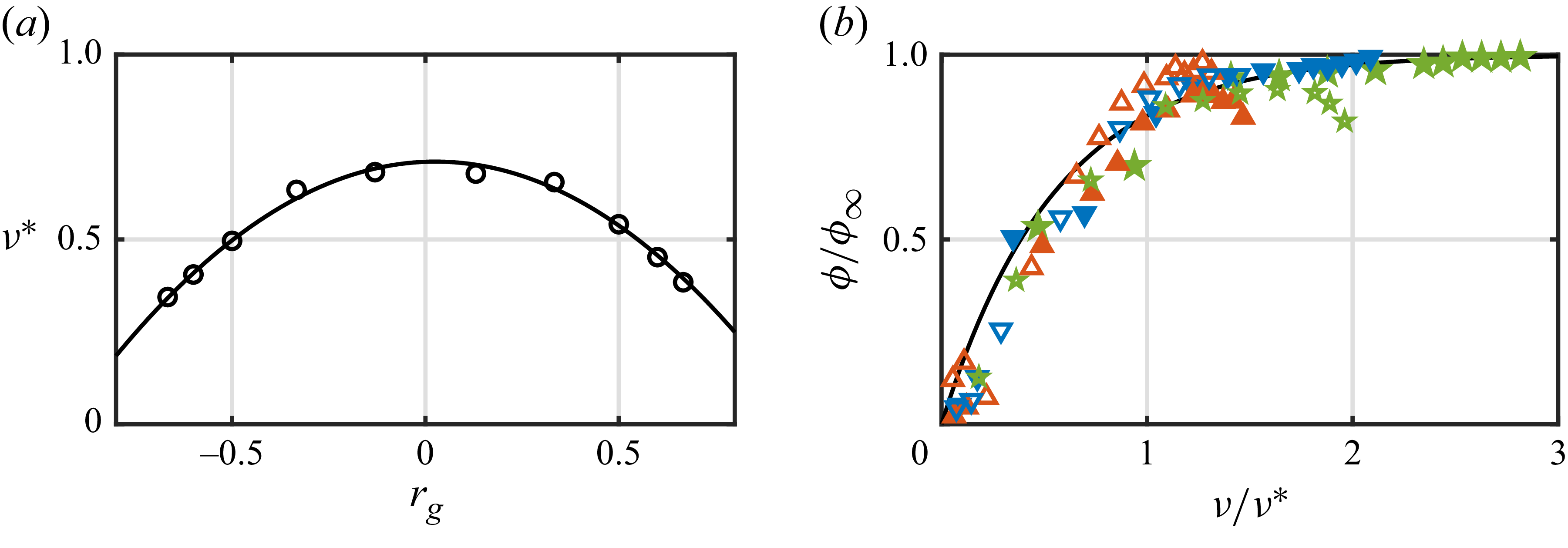


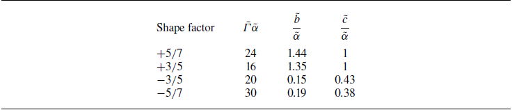

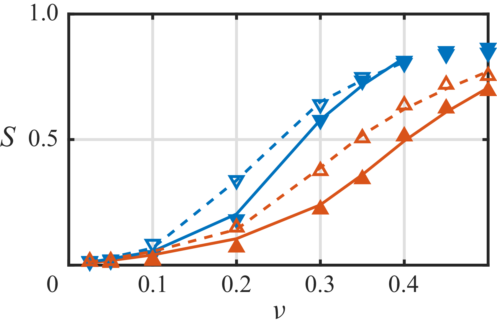


 Open access