


The optimal design of central bank intervention in the face of economic and financial crises has been debated since at least Thornton (Reference Thornton1802) and Bagehot (Reference Bagehot1873). Recent theory and policy discussions have paid some attention to the beneficial role of broad access to central bank operations and a broad definition of eligible assets, see, among others, Cúrdia and Woodford (Reference Cúrdia and Woodford2011) and BIS (2013). We empirically show that granting broad and direct access to the central bank better stabilizes the economy compared with a counterfactual situation in which the central bank intervenes through a small number of eligible counterparties or allows only a restricted subset of financial assets to be used as collateral in its liquidity operations.
Our empirical setup overcomes the three factors that usually impede the quantitative assessment of eligibility frameworks, namely the fact that crises are rare events, potential reverse causality, and confounding factors. We exploit the spread of phylloxera, a pandemic that devastated French vineyards during the nineteenth century. The pandemic amounted to a negative supply shock in agriculture and consequently caused a negative demand shock in the other sectors of the economy (Guerrieri et al. Reference Guerrieri, Lorenzoni, Straub and Werning2022), triggering an increase in the default rates of non-agricultural firms. Against this background, we show that the Bank of France reduced the number of defaults in districts where it de facto extended its liquidity support to more agents and more assets, compared to districts in which it allowed a smaller proportion of agents and assets to access its liquidity facility.
In order to isolate the effect of eligibility on economic outcomes, an empirical test requires a negative shock that is not explained by agents taking more risks in expectation of having access to the lender of last resort facility (thus excluding moral hazard). In addition, the shock must hit several economies that differ with respect to the degree of eligibility to the central bank but otherwise are all subject to identical monetary and fiscal policies. We claim that a quasi-natural experiment in nineteenth-century France combines these ingredients.
Starting in 1863, France was hit by a series of negative productivity and capital shocks that affected French départements (districts), each being of a size equivalent to an average U.S. county, at different points in time. The shock was brought about by an agricultural disease caused by the insect phylloxera. Phylloxera killed nearly all of the vines in an economy in which wine production was both important and widespread (Banerjee et al. Reference Banerjee, Duflo, Postel-Vinay and Watts2010). Wine production decreased significantly. The agricultural productivity shock translated into an aggregate shock on local banking systems as well as services and industry (Postel-Vinay Reference Postel-Vinay, Grantham and Leonard1989).
To identify the effects of eligibility for central bank operations, we exploit a peculiarity of nineteenth-century central bank operations, where eligibility was tied to geographical criteria and thus differed across districts. As the arrival and spread of phylloxera was an exogenous event, we can rule out that the crisis was triggered by moral hazard behavior linked to expectations of eligibility extensions. Finally, we can exclude a potential counter-cyclical impact of fiscal and monetary policy as neither the French government nor the central bank intervened (Bignon, Caroli, and Galbiati Reference Bignon, Caroli and Galbiati2017).
Our analysis uses a uniquely rich set of hand-collected administrative data documenting the number of defaults and the stock of non-agricultural firms in each of the 85 districts, as recorded by the ministries of justice and finance. We also have information on the inclusiveness of the eligibility rule at the district level. Our panel includes yearly data spanning the period 1851 to 1913. We run two types of panel regressions. First, we show that the crises of local economies triggered by phylloxera significantly increased defaults of non-agricultural firms. Second, we regress the default rate of non-agricultural local firms on the depth of the local economic crisis, a measure of the inclusiveness of the eligibility for central bank operations, and an interaction term.
The results show that districts with broader eligibility for central bank operations experienced a less marked increase in the default rate of non-agricultural firms than did districts with stricter eligibility rules. The preferred specification suggests that phylloxera triggered an increase of about 20 percent in the default rate of non-agricultural companies, but this effect was partially dampened when the Bank of France operated a wider discount window. The results are robust across various specifications and to the correction for spatial autocorrelation in the error terms. We rule out that eligibility was endogenous by showing that variations in eligibility at the district level were uncorrelated with the spread of the disease, measures of the economic crisis triggered by phylloxera, or variations in the district default rate. Finally, we show that the central bank did not make losses on its extended discount operations. The observed decrease in the default rate was due solely to central bank eligibility rather than a quasi-fiscal subsidy by the central bank.
Our results inform first about the importance of the design of central bank liquidity injections in times of crisis, in addition to and independently of the amount of liquidity provided. Following Friedman and Schwartz (Reference Friedman and Schwartz1963), the literature on central bank intervention has focused on the quantity of monetary injections. Richardson and Troost (Reference Richardson and Troost2009) show that the generous liquidity provision by the Atlanta Fed during the Great Depression stabilized the economy better than the restrictive discount window policy of St. Louis; see Ziebarth (Reference Ziebarth2013) and Jalil (Reference Jalil2014). Carlson, Mitchener, and Richardson (Reference Carlson, Mitchener and Richardson2011) exploit a real negative shock on the Florida economy to show that liquidity provision can halt bank failures. Compared to those papers, ours adds two features of an ideal research design: we exploit a real shock to the economy to study a negative demand shock and use variations in policy implementation to make visible the non-monetary effect of central bank intervention, which is related to the eligibility for those injections and not to the quantity of money provided. In other words, the paper identifies the positive effect of a change in the composition of the monetary injections into the economy.
Another contribution of the paper is the evidence on the economic significance of being eligible to the central bank. Starting with White (Reference White1983), the economic history literature has had a long-standing interest in the reasons why U.S. banks joined the Federal Reserve System or, possibly more puzzling, why many decided not to. The trade-off highlighted in this literature is between, on the one hand, the potential regulatory cost for banks when becoming a member of the Fed (instead of remaining under more lenient state regulations) and, on the other hand, the benefits of access to the discount window (i.e., the shadow price of liquidity in crises times), see Mitchener and Richardson (Reference Mitchener and Richardson2018) and Anderson et al. (Reference Anderson, Calomiris, Jaremski and Richardson2018) for recent contributions. Those studies highlight the financial stability consequences of narrow eligibility and reduced lending that follows bank failures. Our research design allows us to overcome the empirical challenge of self-selection inherent to the U.S. case. Unlike in the United States, there was no banking regulation in France during the period of our study, and entry into banking was free. This allows showing that eligibility for the central bank mattered for the economy as a whole, as default risk was reduced.
Our paper also sheds light on the recent debate in macroeconomics on the respective role of fiscal versus monetary policy when an economy is hit by a negative supply shock. Triggered by COVID, this literature highlighted how a negative supply shock in some sectors induced a negative demand shock in others (Guerrieri et al. Reference Guerrieri, Lorenzoni, Straub and Werning2022; Woodford Reference Woodford2022). Both models advocate for targeted fiscal transfers, and Woodford (Reference Woodford2022) shows that interest rate policy is not an effective tool for stabilization. In contrast, our paper provides empirical evidence that, when faced with negative externalities between sectors, monetary policy can play a positive role. In particular, in a context in which fiscal policy was inactive, we show that eligibility to the central bank potentially relieved part of the burden of adjustment.
Our unique setup is characterized by the long duration of the economic slump and by an equivalently long central bank intervention. This may seem at odds with a standard view on liquidity provision by the central bank. In this view, lender-of-last-resort policy is understood as being necessarily short-lived. Our empirical setup stresses another aspect of lending-of-last-resort, namely the general knowledge that a broad discount window is available, which agents can use in times of stress to convert part of their wealth into currency. Already, Bagehot (Reference Bagehot1873) argued that the firm commitment of the central bank to continuously operate its discount window will dampen financial panics or prevent them from even arising. Our paper adds empirical evidence that this commitment was more effective when eligibility was defined more broadly.
Finally, our results contribute to the economic history of France. We add to Banerjee et al. (Reference Banerjee, Duflo, Postel-Vinay and Watts2010) and Bignon, Caroli, and Galbiati (Reference Bignon, Caroli and Galbiati2017) by showing the macroeconomic shock that phylloxera had on the local French economy. We are also the first to show that central bank branches played an important role in stabilizing local macroeconomies, contrary to the traditional views that underline the political or competitive motives in the building of the branch network, see Pose (Reference Pose1942) and Bouvier (Reference Bouvier1973).
HISTORICAL BACKGROUND
We describe how phylloxera induced local economic crises before discussing the difficulties that private agents faced when using the financial system to smooth income shocks and explain how a peculiarity of the debt contracts purchased by the central bank can be exploited in our empirical strategy.
Crises: Phylloxera, the Bug That Shocked Local Economies
The first ingredient in our quasi-experimental setting is the sizeable negative productivity shock brought about by the arrival of an agricultural disease in an economy dominated by agriculture. Once the disease arrived in a district, it started destroying the vineyards, reducing local wine production, and making wine growers poorer (Banerjee et al. Reference Banerjee, Duflo, Postel-Vinay and Watts2010; Bignon, Caroli, and Galbiati Reference Bignon, Caroli and Galbiati2017).
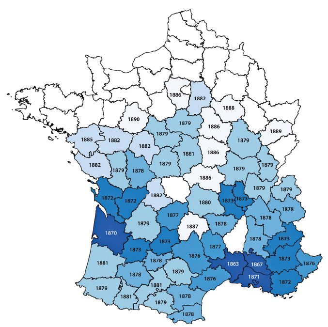
The disease was caused by the near microscopic aphid Phylloxera vastatrix—literally the killer of the vineyard—which sinks its pointed snout into the roots of the vine and sucks out the sap. Its saliva infects the roots, preventing the wound from healing. In this way, phylloxera not only causes yields to fall to zero, but also kills the entire plant within a short period of time. The approximate length of time between the arrival of the pest and the death of the plant was about a year (Pouget Reference Pouget1990). Phylloxera started infecting French vineyards in 1863 near the Rhône River in the south of France and soon thereafter in the Bordeaux region (Gale Reference Gale2011, p. 18). It then spread gradually but irregularly across the territory (Figure 1). Even within districts, the speed of destruction was not uniform across time and space. For example, between 1871 and 1879, the southeastern district of Gard lost 83 percent of its vineyards, while neighboring Hérault lost 59 percent—nonetheless, a substantial number (Lachiver Reference Lachiver1988, p. 416).
THE SPREADING OF PHYLLOXERA ACROSS FRENCH DÉPARTEMENTS
Source: Galet (Reference Galet1957).

Figure 1 Long description
The map of France illustrates the spread of phylloxera across various departments, with each department labeled with the year it was affected. The map uses different shades of blue to indicate the progression of the infestation over time, with darker shades representing later years. Key departments such as those in the south and southeast show earlier years like 1863 and 1871, while northern and eastern departments show later years like 1882 and 1889. This visual representation highlights the chronological spread of phylloxera across the country.
Regressions that identify the dynamic effect of phylloxera over time, along the lines of Wolfers (Reference Wolfers2006) show that, on average, phylloxera started to have a significant negative effect on wine production four years after the first sighting of the aphid in a district.Footnote 1 The coefficients imply that, after controlling for time and district fixed effects, wine production declined by about 37 percent after five years and by 66 percent after ten years, relative to the last year before phylloxera.
It took a long time to understand why the vines were dying and even longer to understand what could be done about it. The insect was first hypothesized as an explanation for the dying vines in 1868, after the study of a dead vineyard near the Rhône by botany professor Jules E. Planchon. Following identification, a debate raged for seven years before the scientific community agreed that the appearance of the bug was, in fact, the cause and not merely a consequence of the disease. None of the various treatments to fight the pest proved helpful (Pouget Reference Pouget1990). It was only in 1890 that a cure was found and popularized. The solution involved grafting European vines onto phylloxera-resistant American stock.
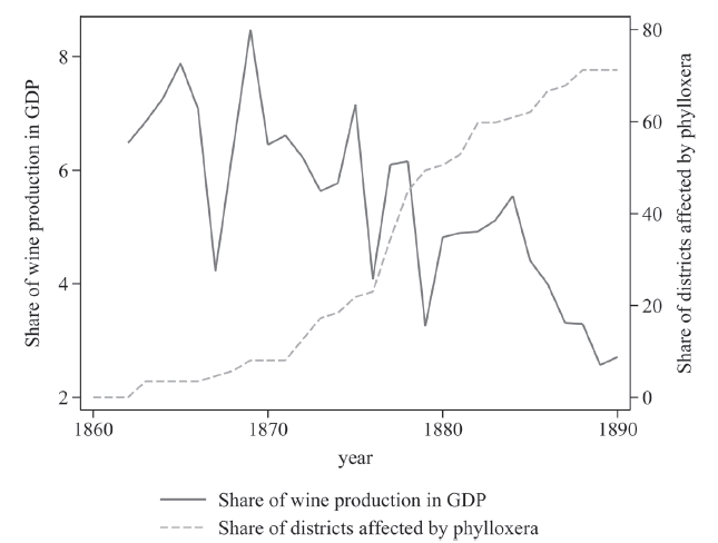
Phylloxera caused a sharp drop in revenues. The share of wine production amounted to 6.4 percent of pre-aphid 1862 French GDP, declining to 2.75 percent of GDP in 1890 (see Figure 2). While wine represented a source of income for 21 percent of the population in 1870 (Millardet Reference Millardet1877, p. 82), its importance and therefore the impact of phylloxera varied across districts. On average, wine production represented 9.2 percent of GDP in wine-producing districts, but it could reach up to 54 percent in some.Footnote 2 In those regions, the impact of the aphid on local economies was disastrous (Postel-Vinay Reference Postel-Vinay, Grantham and Leonard1989), even more so as price increases did not compensate for the fall in quantity.Footnote 3 The fall in revenues caused local economic distress. Using regressions again to estimate the dynamic effect of phylloxera, this time on default rates, we see a significant increase five years after the first spotting of phylloxera.Footnote 4 Calculated at the average size of the phylloxera shock, the coefficients imply an increase in the default rate of 2.5 percent five years and 6.8 percent ten years after the first spotting of phylloxera (thus one and six years respectively after the illness had led to a significant decrease in the wine production of the infected district). Note that this magnitude is the average of districts with and without access to the mitigating facilities of the Bank of France.Footnote 5
REVENUES FROM WINE PRODUCTION AS PERCENT OF GDP AND THE SHARE OF WINE-PRODUCING DÉPARTEMENTS INFECTED BY PHYLLOXERA, 1860–1890
Source: Authors’ representation based on Bignon, Caroli, and Galbiati (Reference Bignon, Caroli and Galbiati2017).

Figure 2 Long description
A two line graph shows the share of wine production in GDP and the share of districts affected by phylloxera from 1860 to 1890. The x axis represents the years from 1860 to 1890. The left y axis represents the share of wine production in GDP, ranging from 0 to 8. The right y axis represents the share of districts affected by phylloxera, ranging from 0 to 80. The solid line represents the share of wine production in GDP, which fluctuates significantly over the years, peaking around 1870 and then declining sharply around 1880 before stabilizing at a lower level. The dashed line represents the share of districts affected by phylloxera, which starts low around 1860, gradually increases, and then rises sharply around 1880, continuing to increase until 1890. All values are approximated.
The length of the episode made it impossible for farmers to maintain consumption by drawing on their savings and very unlikely that farmers were able to increase their savings in advance. This would have required a clear understanding of how the disease would spread and of its cause, an issue not settled before 1875 (Gale Reference Gale2011). Even then, historical evidence shows that the newly reached agreement on the cause of the disease did not make French peasants any wiser when it came to anticipating future losses.
In 1881, the inspector of the Bank of France visiting the branch in Perpignan, at the heart of the wine region Roussillon, was still boasting with optimism: “The country is rich: since 1869 wine production has tripled in spite of the progress of phylloxera. […] Fortunes are growing by the day, one lives simply and inventories of 100 to 150 thousand francs are not rare.” Note that the inspector mentioned phylloxera, but did not recognize the looming catastrophe, in spite of examples like the nearby district of Hérault. Barely a year later, the report read entirely differently: “This land […] sees bad years coming. Out of a total of 75,000 hectares of wine, 10,000 have been destroyed in 1881, 15,000 in 1882 and 50,000 are attacked by phylloxera. The disappearance of wine […] is just a question of time and production will seize.”Footnote 6 Historiography identifies two reasons for this lack of foresight. Some peasants believed that the disease would be confined by nature to certain regions, while others simply denied its existence, arguing that the disease could be avoided by taking good care of the vines (Gale Reference Gale2011, p. 52). Loubere (Reference Loubere1978, p. 158) traces the blindness to the policy of uprooting the diseased vines as a means of safeguarding those that remain intact.
The impact of phylloxera on farmers and agriculture was countered neither by fiscal nor monetary policy. Before 1898, the central bank was prohibited from purchasing any assets that originated in the agricultural sector (Baubeau 2011). Fiscal policy was of little help either: at the apex of the disease in the 1880s, the state spent a million francs a year on phylloxera—the equivalent of 0.7 percent of France’s 1862 wine production—and this little money was directed toward scientific research (Loubere Reference Loubere1978, p. 172). No welfare programs, such as unemployment or turnover-loss benefits, existed to absorb revenue losses.
The Financial System in the Face of Phylloxera
During the first years, farmers smoothed the shock by borrowing from local credit markets intermediated by notaries (Postel-Vinay Reference Postel-Vinay1998). But the failures of farmers and wine growers fed back to notaries and to the savers who had entrusted funds to them. Some notaries failed, and savers shied away from investing in assets originating in the agricultural sector (Postel-Vinay Reference Postel-Vinay1998, pp. 286–87). In addition, the liquidity of mortgages and other long-term debts was hit, as defaults on interest payments limited the possibility of reselling them on the secondary market (Postel-Vinay Reference Postel-Vinay1998, pp. 325–26). Farmers turned to other financial intermediaries, such as local banks, to borrow, but these were impacted by the crisis as well (Postel-Vinay Reference Postel-Vinay, Grantham and Leonard1989). As a result, the shock created by phylloxera in agriculture was transmitted to other economic sectors and decreased revenues there.
Firms outside agriculture were also affected by the declining availability of notarial credit. The main alternative was bills of exchange, which were negotiable and could be re-discounted at the central bank, making them especially liquid. The business of discounting bills was not regulated and was open to everybody (Kaufmann Reference Kaufmann1914; Plessis Reference Plessis1991). Bills of exchange were considered very safe, as the legal framework imposed high costs in case of failure, meaning that strategic default was hardly an option.Footnote 7 Yet, what was an advantage in normal times also created a mechanism that could amplify the consequences of defaults in times of crisis and might lead to a sudden drying up of liquidity in the bills market (Bignon and Flandreau Reference Bignon and Flandreau2018). Indeed, the double liability rule associated with the discounting of bills could trigger, in times of stress, a chain of defaults. The risk for such an outcome was aggravated by the absence of a preferential treatment for bills in the failure procedure, forcing guarantors of the bill to pay immediately while having to wait until the end of the procedure to recuperate (most) of their claims (Percerou Reference Percerou1935). Given the normal length of such procedures of about two years, any exogenous increase in defaults increased the share of illiquid debts and hence the likelihood of being unable to pay debts in due time.
Anecdotal evidence abounds that when payment incidents started, it was difficult to interrupt the chain because of the stay of creditors in a lengthy procedure and the impossibility of exiting it before its legal termination (Cameron Reference Cameron1967). As bills of exchange also served as a means of payment, cascades of defaults threatened the payment system as well. Gille (Reference Gille1959) provides evidence that in times of financial stress, local market discount rates skyrocketed in small towns where no discount facility was operated by the Bank of France. These rates, which measured the price of converting short-term credit instruments into coins or banknotes, occasionally attained levels as high as 18 to 30 percent (Gille Reference Gille1959, pp. 145–48).
The Bank of France as Provider of Liquidity
When the payment system was threatened by this type of difficulty, bankers and traders could turn to the standing facilities operated by the Bank of France. The Bank purchased bills of exchange outright (Leclercq Reference Leclercq2010).Footnote 8 As banking was not legally defined, the Bank of France could not restrict discounting to “banks,” and all firms active in banking, services, and industry could, in principle, submit bills to the Bank of France. The only sector excluded was farming until the rules were amended in 1898, well after the end of the phylloxera crisis (Baubeau 2011).
The Bank of France did not buy bills on a market through open-market operations. Rather, discounting was organized as a standing facility open in all its offices. Its incorporation law restricted the Bank to buying bills maturing within three months following their purchase. The price was determined by the bill’s face value minus the discount rate times the residual maturity. By law, the discount rate was uniform across France and could not be adjusted to local conditions or the risk profile of counterparties.
The Bank’s policy during crises was to accommodate any increase in demand for refinancing from sound traders (Juglar Reference Juglar1889; Bouvier Reference Bouvier1973). From the 1850s, the Bank implemented Bagehot’s rule of free lending against collateral considered to be of good quality in normal times (Bignon, Flandreau, and Ugolini Reference Bignon, Flandreau and Ugolini2012). Due to its sizeable gold and silver reserves, the requirement to convert banknotes on demand did not constrain the aggregate volume of refinancing (Flandreau Reference Flandreau1996; Contamin and Denise Reference Contamin and Denise1999).Footnote 9 Refinancing volumes and the discount rate were set by the Bank’s governing body, in which private shareholders enjoyed a two-thirds majority over the representatives of the government (Plessis Reference Plessis1985). Finally, in the period under consideration, eligibility rules at the discount window were severe in terms of both screening and monitoring of the Bank’s counterparties (Avaro and Bignon Reference Avaro and Bignon2019). Moreover, the Bank of France did not hesitate—in case of a failure of counterparties—to sue the defaulters in court and enforce full repayment.
Geographical Constraints on the Eligibility of Assets at the Bank of France
In this section, we detail the specifics of discount window operations to derive the exogenous measure of eligibility used in the regression analyses later. In this regard, the most interesting feature of the discount window was the legal requirement for the owner of the bill to physically go to the debtor’s door and collect payment. The possibility of buying and holding bills to maturity was thus constrained by the size of the area that could be reached by payment collectors.Footnote 10 It followed that only bills payable in towns in which the Bank of France maintained a team of collectors were potentially eligible for its discount window. As a result, the share of local traders eligible for the discount window varied across districts.
As this technology did not change significantly over the whole of the nineteenth century, the extension of assets eligible for discounting was directly tied to the establishment of new local collection facilities. Between 1815 and 1836, the only office operated by the Bank of France was in Paris, which restricted discounting to bills payable in Paris. In the following decades, the Bank successively opened more and more offices across France. Starting in 1882, the Bank complemented the existing succursales (subsidiaries) with a second type of branch, the bureau auxiliaire (auxiliary office), see Brouilhet (Reference Brouilhet1899) and Leclercq (Reference Leclercq2010). Auxiliary offices were subordinated to the succursales and did not enjoy the same leeway when it came to discounting. According to the hearing of then Governor Pallain before the U.S. National Monetary Commission, “the auxiliary offices are subjected to the same regime as the branches, except as concerns discount” (Aldrich Reference Aldrich1910, p. 192). Regarding eligibility, only subsidiaries could decide which bills qualified for a discount. Moreover, it was only the subsidiaries that were organized to collect payments on due day on any working day of the week.Footnote 11 In the following, we therefore focus on the subsidiaries.
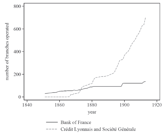
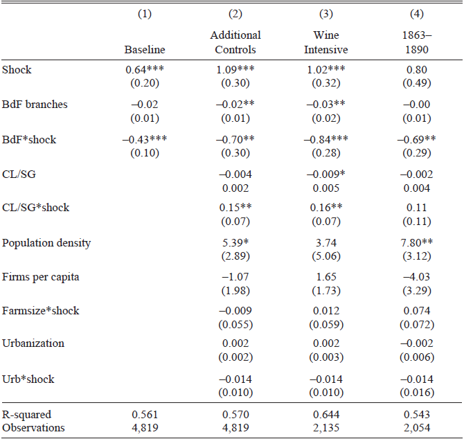
Figure 3 presents the evolution of the number of subsidiaries operated by the Bank of France between 1851 and 1913. The gradual extension of the branch network not only allowed more agents to become eligible as a counterparty of the Bank but also made more bills eligible, thereby extending the share of assets—among all assets—against which central bank money could be obtained. At the same time, certain districts had to wait a long time for a branch office, and many towns never obtained one, as the fixed cost of setting up and operating branches prevented the Bank from opening them everywhere. In 1913, the number of branches in each district varied between one (in mostly agricultural districts) and nine (in the highly industrial “Nord” district). The uneven distribution of branch offices across France—it was only in 1877 that the Bank of France was present in every French district—creates variations in eligibility over both time and space.
NUMBER OF BRANCHES OF THE BANK OF FRANCE AND THE TWO MAIN NATIONAL DEPOSIT BANKS, 1830–1913
Source: Banque de France, Comptes rendus.

Figure 3 Long description
A line graph showing the number of branches operated by the Bank of France and two main national deposit banks from 1830 to 1913. The x-axis represents the years from 1840 to 1920, and the y-axis represents the number of branches operated, ranging from 0 to 800. The solid line represents the Bank of France, while the dashed line represents Credit Lyonnais and Societe Generale. The graph shows a gradual increase in the number of branches for the Bank of France from around 1840 to 1920, with a noticeable rise starting around 1880. The dashed line, representing Credit Lyonnais and Societe Generale, shows a more rapid increase starting around 1860, with a significant rise after 1900, reaching close to 800 branches by 1920. All values are approximated.
The only other type of financial institution that had the organization and technology to potentially smooth regionally concentrated illiquidity-driven defaults by redistributing liquidity across districts was the two deposit banks that operated on a national level, that is, the Crédit Lyonnais and the Société Générale. From the 1860s onward, these two banks developed extensive networks of branches, with the aim of collecting deposits and attracting prime bills at their discount windows, see Bouvier (Reference Bouvier1973) and Lescure (Reference Lescure, Feiertag and Margairaz2003), though their networks only came to match the Bank of France by the early 1880s. Technically, both were capable of increasing discounting in branches located in districts affected by a crisis using the deposits from unaffected districts, very much like the Bank of France could resort to issuing banknotes.Footnote 12 In the regression analysis, we therefore control for the presence of national deposit banks.Footnote 13
To sum up, the shock brought about by phylloxera provides an ideal setting for analyzing the effects of variations in central bank eligibility. (i) Phylloxera was a sizable real productivity shock on the agricultural sector and was transmitted to other sectors. (ii) The fact that phylloxera arrived in different districts at different points in time allows us to analyze the effects of the crisis at a district level, thereby increasing the number of observations and helping us to circumvent the small sample problem typical of other lending of last resort studies. (iii) It is reasonable to regard the disease as a temporary income shock on banks, services, and industry, as a cure to the disease was finally found. (iv) The setting properly singles out the role of eligibility, while fiscal policy and other aspects of monetary policy were not changed in response to the shock. (v) The clearly external nature of the shock allows us to rule out reverse causality between eligibility and the economic crises caused by the disease.
EMPIRICAL STRATEGY
Our goal is to determine whether variations in the proportion of assets or agents eligible for the central bank discount window had an impact on the variation in the default rate of banks, services, and industry at the district level when the economy was hit by the phylloxera crisis. We estimate this relation using a difference-in-differences approach. Our main equation is the following:

where DR it stands for the default rate in district i during year t of banks and firms operating in services or industry. The explanatory variables are Shock it, which measures whether the district was hit by the phylloxera shock in district i during year t, Elig it BoF, which measures the exposure of district i to the treatment during year t, and the interacted term Shock it ∗ Elig it BoF, which is the product of the variable Shock it with variable Elig it BoF. Moreover, because the Bank of France was not the only potential local provider of liquidity, we include Elig it FIs, which is a measure of eligibility for national deposit banks, as an alternative source of funding through which the impact of the shock could have been smoothed. The coefficient on the interaction term γ therefore pins down the specific effect of the lending of last resort services through greater eligibility, even after taking the refinancing activities of other financial intermediaries into account. A vector of controls, Controls it, is added to account for other determinants of the default rate in district i during year t. It includes the population density of the district, the urbanization rate, the density of firms in services and industry in the district, and the average size of the individual vineyard in the district, as all of these can individually impact the default rate of the district during year t. All residuals are clustered at the district level.
We are interested in knowing whether the γ coefficient in front of the interacted term Shock it ∗Elig it BoF is significant and negative or insignificant. Our identification assumption is that, in the absence of any friction, the eligibility framework should not have any impact on the default rate of firms since everybody can trade their holdings of non-eligible assets for assets eligible at the discount window at no cost. This follows from the theories developed by Wallace (Reference Wallace1981) and Goodfriend and King (Reference Goodfriend and King1988), who show that it is necessary and sufficient for the central bank to provide the appropriate quantity of money through open-market operations, leaving to the market the task to distribute it to individual banks.
Conversely, if there are some externalities on the money or payment market, like in Flannery (Reference Flannery1996), Acharya, Gromb, and Yorulmazer (Reference Acharya, Gromb and Yorulmazer2012) or Heider, Hoerova, and Holthausen (Reference Heider, Hoerova and Holthausen2015), we expect γ to be negative and significant, since some agents holding non-eligible assets are unable to exchange them for money, and hence may have to default. To show the non-neutrality of the way money is injected in the economy, Flannery (Reference Flannery1996), Acharya, Gromb, and Yorulmazer (Reference Acharya, Gromb and Yorulmazer2012), Shleifer and Vishny (Reference Shleifer and Vishny2010) and Heider, Hoerova, and Holthausen (Reference Heider, Hoerova and Holthausen2015)—among many others—depart from a frictionless model and consider some form of imperfect competition to show that some form of discount policy can be a very effective tool to stabilize financial crises. Notice that this type of effect comes only from a composition effect—a change of eligibility—and does not require an increase in the quantity of money injected in the economy. In macroeconomics, this refers to the debate on the effect of quantitative easing vs. credit-easing policy, see Cúrdia and Woodford (Reference Cúrdia and Woodford2011).
The spatial structure of the data might raise concerns about the correlation of the error terms between districts, which, in turn, might bias the estimated coefficients or change the standard errors. For example, there might be determinants of the dependent variable that were omitted from the model but that are spatially autocorrelated, meaning that the error term is correlated between nearby districts. To show the robustness of our result to spatial autocorrelation, we estimate the following model:

Equation (2) is identical to Equation (1) with the difference that the error term λW·µ t + ε it allows for spatial correlation between error terms. W denotes a spatial weights matrix based on the distance between the administrative centers of the districts, where we assume a declining impact of errors from districts that are further away. λ measures the extent of spatial correlation, where zero means that there is no spatial correlation, and a higher λ means stronger spatial spillovers.
DATA
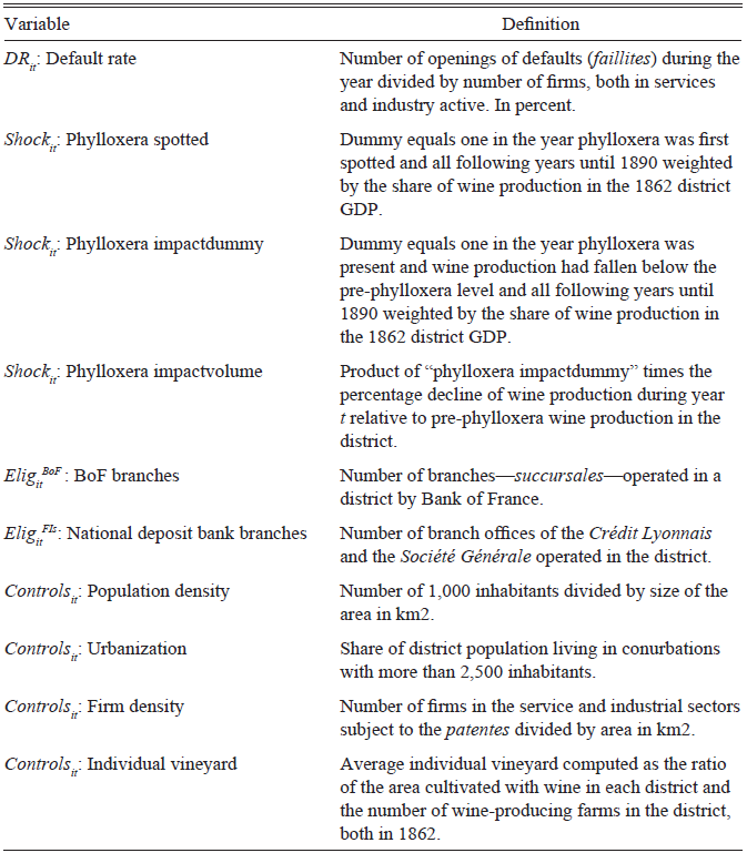
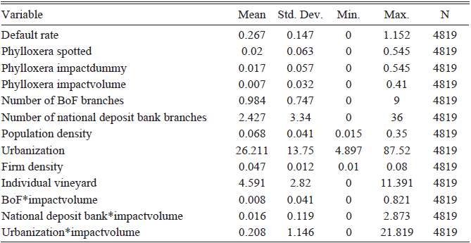
The dataset contains yearly observations on the variables of the equation: the default rate, yearly measures of the magnitude of the shock triggered by the spread of phylloxera in each district, and measures of eligibility for the central bank and the two main deposit banks (Table 1). Online Appendix B provides further details on the construction of the database.
DEFINITION OF VARIABLES

Table 1 Long description
The table presents definitions for various variables used in a dataset. It includes columns for variable names and their corresponding definitions. The variables cover default rates, phylloxera impact measures, and the presence of bank branches. Each variable is described in detail, explaining how it is calculated or determined. The table provides a clear and structured overview of the variables used in the analysis.
Source: Authors’ compilation.
Default Rate
The default rate is computed by dividing the number of defaults by the stock of firms in services and industry that are active during each year in each district. For each district and each year, the number of defaults on debt repayment is known from the number of openings of a judicial procedure called faillites (failures). Its legal definition has two convenient features for our empirical design.
First, the opening of a failure procedure was tied to illiquidity and not to insolvency, as the law stated that it could be opened only after the observable recognition of a default. This was to prevent anti-competitive behavior or political interference with the running of businesses. Legal scholars made it clear that a presumed state of insolvency, in itself, could not be taken as a motive for the opening of such a procedure since insolvency could only be decided after a proper screening of assets and liabilities of the firm (Percerou Reference Percerou1935). As a consequence, the number of openings of failure procedures identifies the number of defaults in a given location during a given year. Second, the number provides a clean measure of defaults in services and industry, including banks, while workers and other non-traders, such as lawyers and—importantly—farmers, were subject to different legal procedures.Footnote 14
Measures of the Shock Triggered by the Spread of Phylloxera
To account for the size of the crisis at the district level, we construct different specifications of the variable Shock it in Equation (1). They aim to measure the size of the local economic crisis triggered by the disease in district i during year t. The extent of the crisis varied with the importance of wine in the local GDP as well as the spread of the disease within the district. As the speed at which the bug spread within each district varied across districts and time, no single lag structure can account for it, as will be analyzed empirically. To rule out that results are driven by a particular choice of lag structure, we use three alternative variables to measure the size of the phylloxera shock when estimating Equations (1) and (2).
The simplest specification of Shock it is labeled Spotted it. It is the product of two terms. The first term is a dummy that is set to one for all years between the first year the aphid was spotted in the district and the year of the implementation of the cure for the disease in 1890. In any year before the aphid arrived in the district and after the implementation of the treatment in 1890, we set the dummy to zero. In order to account for the varying importance of wine for an economy i, the dummy is multiplied by a second term, which is equal to the share of wine production in the 1862 GDP. As a result, Spotted it is equal to a constant term during the years phylloxera was present in district i and zero otherwise. Table 2 presents the descriptive statistics.
SUMMARY STATISTICS

Table 2 Long description
The table presents summary statistics for multiple variables, including default rate, phylloxera spotted, phylloxera impact dummy, phylloxera impact volume, number of Bank of France branches, number of national deposit bank branches, population density, urbanization, firm density, individual vineyard, and interactions of these variables with impact volume. The table consists of seven columns: Variable, Mean, Standard Deviation, Minimum, Maximum, and N. Each row provides statistical data for a specific variable. For example, the default rate has a mean of 0.267, a standard deviation of 0.147, a minimum of 0, a maximum of 1.152, and a sample size of 4819. The phylloxera spotted variable has a mean of 0.02, a standard deviation of 0.063, a minimum of 0, a maximum of 0.545, and a sample size of 4819. The table provides a comprehensive overview of the statistical distribution of these variables.
Source: Authors’ calculations. For the underlying data, see Bignon and Jobst (2026).
A second measure of the size of the local economic crisis is the variable labeled impactdummy it that controls for the time that could have passed between the first spotting of the aphid in the district and the moment at which it led to widespread devastation of vineyards. We use a dummy variable constructed by Banerjee et al. (Reference Banerjee, Duflo, Postel-Vinay and Watts2010), which is set to one if the following two conditions are fulfilled. First, the aphid is present in the district. Second, wine production has fallen below the level reached during the last year before the arrival of phylloxera. In the absence of direct information on the spread of the aphid within each district, this condition aims to capture that phylloxera must have spread sufficiently widely to have had an impact on wine output. Again, the dummy is set equal to 0 after the implementation of the treatment in 1890. As in the case of Spotted it, the dummy is multiplied by the share of wine production in 1862 GDP. As a result, impactdummy it is equal to a constant term during the years when both phylloxera was present in district i and after wine production had declined relative to the pre-phylloxera benchmark level before 1890, and is zero otherwise.
A third alternative, which is our preferred variable, is labeled impactvolume it, which is constructed as a continuous version of impactdummy it by taking into account the actual decline of wine production during the period when phylloxera affected wine production. To construct the measure, we again use a variable constructed by Banerjee et al. (Reference Banerjee, Duflo, Postel-Vinay and Watts2010); this time, however, multiplied by the percentage decline in wine production relative to the level in the last year before the phylloxera was spotted in a district. Therefore, impactvolume it varies with the actual decline in wine production during each year between the arrival of the disease in the district and 1890 and can thus take best account of the district-specific speed with which phylloxera propagated. The advantage of this last specification is that, due to climatic and geographical factors, wine production in some districts may have been more affected by phylloxera than in others. Moreover, impactvolume it accounts better than the other two specifications for the instantaneous impact of phylloxera on local income. The following baseline regressions thus use impactvolume it as the explanatory variable, while spotted it and impactdummy it are employed to check the robustness of the results.
Measuring the Eligibility for Central Bank Lending
To measure the extent of access of local agents to the facilities offered by the Bank of France and the two national deposit banks elig it, we use the number of branches branches#it operated by the Bank of France and the national deposit banks within each district i during year t. Taking the simple number of branches is justified, given that French districts were roughly equal in size and had been designed in 1790 so that every place within the district was within a one-day horse ride from the district’s administrative center.
BRANCHING DECISIONS OF THE BANK OF FRANCE
As discussed previously, a central ingredient of the empirical strategy for identifying the real effects of central bank eligibility is that extensions in eligibility are exogeneous to the economic shock brought by phylloxera. This section now shows that the decision of the Bank of France to open new branch offices (the eligibility variable) was not driven by the concern to alleviate the effects of phylloxera, nor that the Bank hesitated to open branches in districts hit by the phylloxera crisis. We provide both narrative and econometric evidence that branching can be considered exogeneous.
Historians explain the gradual extension of the branch network of the Bank of France, shown in Figure 4, as the outcome of both political and competitive pressures (Pose Reference Pose1942; Bouvier Reference Bouvier1973; Plessis Reference Plessis1985). Having taken over all provincial note-issuing banks in 1848 (Gille Reference Gille1970), the Bank of France enjoyed a monopoly on note issuance in the towns in which it operated a branch. This monopoly was only briefly contested by the Pereires brothers in the 1860s (Cameron Reference Cameron1961; Domin Reference Domin2007). From the 1860s onward, however, some commercial deposit banks, most notably Société Générale and Crédit Lyonnais, created their own large networks, covering the entire territory of France by the early 1880s (Bouvier Reference Bouvier1973; Pose Reference Pose1942). These banks collected significant amounts of deposits that they employed in local discounting, thereby draining business away from the Bank of France (Lescure Reference Lescure, Feiertag and Margairaz2003, pp. 136–37). As competition for good bills was fierce in the larger cities, the Bank of France reacted by expanding its own network and refinancing banks in more remote places (Nishimura Reference Nishimura1995).
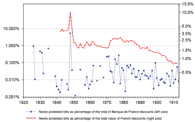
UNPAID BILLS AT MATURITY IN THE ECONOMY AT LARGE AND IN THE DISCOUNT PORTFOLIO OF THE BANK OF FRANCE, 1820–1913 (LOGARITHMIC SCALES)
Sources: Banque de France, Comptes rendus and Roulleau (Reference Roulleau1914) for the entire economy.

Figure 4 Long description
A two line graph depicting newly protested bills as a percentage of the total of Banque de France discounts and the total value of French discounts from 1820 to 1913. The x axis represents the years from 1820 to 1913. The left y axis represents the percentage of newly protested bills as a portion of the total of Banque de France discounts, ranging from 0.001 percent to 10 percent. The right y axis represents the percentage of newly protested bills as a portion of the total value of French discounts, ranging from 0.5 percent to 15 percent. The blue line with dots shows the percentage of newly protested bills as a portion of the total of Banque de France discounts, while the red line shows the percentage of newly protested bills as a portion of the total value of French discounts. The blue line fluctuates significantly, with notable peaks around 1840 and 1870. The red line shows a general decline over time, with a sharp peak around 1850. All values are approximated.
A second motive for the opening of branches was politics. The charter—in particular, the note-issuing monopoly—was granted to the Bank for specified periods of time (Ramon Reference Ramon1929). Whenever the charter came up for renewal, the Bank needed political support from the government and lawmakers (Dauphin-Meunier Reference Dauphin-Meunier1936). Extending services at existing branches or opening new branches was a good way of buying support at the local level. As a consequence, all renewals included clauses that led the Bank to extend its network. The renewal of the privilege of 1857 required the Bank to open at least one branch in every district without setting a deadline. The deadline was added in 1873, when the Bank was instructed to cover all districts by 1877 at the latest (Plessis Reference Plessis1985, pp. 199–201). The charters of 1897 and 1911 again contained clauses requiring the opening of further branches (Pose Reference Pose1942). In addition, according to Lescure (Reference Lescure, Feiertag and Margairaz2003), from the 1880s onward, a new generation of bank officers saw the role of the Bank as being at the service of the public and, hence, with an obligation to ensure equal access to its services for all citizens.
The opening of a branch was costly. In the 1890s, the Bank estimated the set-up costs to be about 160,000 francs, and the annual operating costs at 36,000 francs for a small branch, at a time when the hourly wage of a qualified blue-collar worker rarely exceeded one franc. Given the high set-up costs, the Bank had to seriously consider the long-run viability of a new branch by obtaining information on the likely volume and risk characteristics of the local demand for (re)discounting. The opening of a branch also took time. The Bank had to find a building and recruit a director and staff, as well as the members of the committee that examined the bills submitted for discounting. Opening a branch office typically required a lead time of one year and could hardly be used to address an acute crisis.
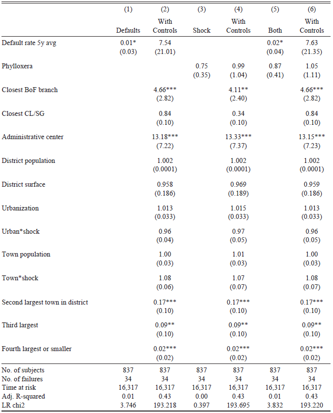
The network expanded gradually until the mid-1880s and was then extended significantly after 1897 and 1911, see Figure 3. This pattern aligns well with both mounting competition from commercial banks in the 1860s and the political economy of rechartering. We estimate a duration model to check this interpretation. The model studies all urban conurbations in France with at least 2,500 inhabitants to estimate which characteristics were significantly associated with the opening of a branch by the Bank of France. The goal is to explain the time it took for the opening of a branch office. Duration analysis is appropriate, as the Bank never closed a branch; in other words, the status of a town can only change from not having a branch to having one. This gives 837 potential cities, among which the Bank of France chose 34 to open a branch during the phylloxera years between 1862 and 1890.
The regression model reads as follows:

Equation (3) explains the opening of a branch in a town j of district i during year t, where opening ijt = 1 if a branch was opened in the town during year t and otherwise is set equal to 0. Previous historical research summarized earlier suggests the inclusion of both political and economic factors as explanatory variables. In addition, we include both an indicator for the presence of phylloxera and the default rate to see whether the spread of the disease and its economic consequences affected the Bank’s behavior. Because it took at least a year between the decision to open a branch and its opening to the public, all right-hand side variables are lagged by one year.
The following economic factors accounted for the attractiveness of establishing a branch in a given town. First, population Pop ijt−1 of the city is a proxy for the size of the local economy. The population of the district Popdistrict ijt−1 measures economic activity in the wider catchment area of a potential branch office, while the inclusion of the surface of the district surface ij corrects for low or high population density. Urbanization is included to account for the economic structure of the district. Competitive pressure is measured by the distance to the closest branch of a national deposit bank branch during the previous year Bank ijt−1, the variable being zero if there is a branch in the very town where the Bank is contemplating opening an office.
The political variables capture the pressure coming from the need for a regular renewal of the charter. The 1857 charter, reinforced in 1873, required the Bank to open at least one branch in every district. As a consequence, the probability of a branch opening should be higher in those districts where the Bank has no branch office yet. The dummy variable BoFpresent jt−1 is zero if the Bank of France has no branch office in this town or in any other town of the district and one otherwise. Given that the 1857 charter of the Bank of France forced the Bank to open a branch in every district before 1878, it is likely that the bank would do so in the economically most important town of the district. This is accounted for by the variables poprank1, …, poprank3, which are set to one for the largest to the third largest, and poprank4 to the fourth largest or smaller city in the district. Dummy CapCity ij indicates whether the town is the administrative center of the prefecture (district).Footnote 15 It accounts for the possibility that political pressure would lead to the opening of a branch office in a politically important town.
Finally, we include two variables that look at the impact of local economic shocks and phylloxera in particular. Shock jt−1 is a dummy indicating whether the district was contaminated by phylloxera during the previous year. The default rate DR it−5t−1 is included to check whether local economic crises increased or decreased the Bank’s willingness to operate a local facility. To smooth year-on-year variations, the default rate was averaged over the last five years from t−5 to t−1. Due to a lack of data at the town level, the default rate and the shock variable are measured at the district level. In addition, town population Pop ijt−1 and urbanization are interacted with the shock variable Shock jt−1 to allow for the possibility that larger towns and more urbanized districts could either do better or worse when faced with phylloxera, thereby affecting the Bank’s calculus for opening a branch office.
Table 3 presents the results of the estimations. Coefficients larger than one imply that the variable increases the probability of a branch being opened. Importantly for our argument, the district default rate and the phylloxera crisis variable are not significant, regardless of whether they are included alone or together, and whether further controls are added or not. In terms of economic factors, the coefficients on population and urbanization, as measures of local economic development, are larger than one, as expected, but not significant. What matters is competition, as places closer to existing deposit bank branches are more likely to receive an office of the Bank of France. The coefficient on the absolute population of the town itself is not significant; population rank, however, is. The probability of a branch being opened in the second or third largest town of a district is less than a third of that in the largest city and declines rapidly when we get to the fourth largest conurbation or smaller. The significance of rank reflects the tendency of the Bank of France to open branches in the biggest city in the district, given the constraint that the Bank had to open at least one branch in every district. As soon as one branch had been opened, the probability of further branches being created nearby declined significantly, as evidenced by the coefficient on BoFdist jt−1 being larger than one (and thus yielding a smaller factor as distance declines). Lastly, being a district’s administrative center increases the probability of a branch opening by a factor of about ten.
BANK OF FRANCE BRANCHING EXOGENOUS TO PHYLLOXERA AND DEFAULTS, 1862–1890

Table 3 Long description
The table presents the results of estimations on the factors influencing the opening of Bank of France branches from 1862 to 1890. It includes six columns with different models: Defaults, With Controls, Shock, With Controls, Both, and With Controls. Key variables include the default rate over five years, phylloxera, proximity to the closest Bank of France branch, proximity to the closest credit and savings institution, administrative center status, district population, district surface area, urbanization, urban shock, town population, town shock, and the rank of the town in the district. The table shows that the default rate and phylloxera are not significant factors. Economic factors like population and urbanization are not significant either. Competition from existing branches is a significant factor, with closer proximity increasing the likelihood of a new branch. The population rank of the town matters, with the largest towns being more likely to receive a branch. Being an administrative center significantly increases the probability of a branch opening.
Notes: The table presents the estimate of a Cox regression where the dependent variable is the opening of a branch by Bank of France in city i during year t. The main regressors are the average default rate over the last five years and the presence of phylloxera in the district. District population and surface and urbanization are also measured at the district level. The other regressors are at the city level and include whether it is a district capital, the town population, and the rank of the city population among the cities of the district. We also include the geodesic distance between the city and the closest branch of Bank of France and of the closest national deposit bank, as well as the interacted term between the town population and the urbanization rate multiplied by the shock—measured as the presence of phylloxera in the district. We report exponentiated coefficients and standard deviations. Note that standard deviations cannot be compared to the exponentiated coefficients in the usual way to determine statistical significance.
* p<0.1, ** p<0.05, *** p<0.01
Source: Authors’ calculations.
All in all, the results are consistent with the historical narrative that the decisions by the Bank of France to open branch offices were unrelated to the default rate or the spread of phylloxera. The high cost of setting up branches and the difficulty in monitoring the local discounting activity were strong motivations for the Bank of France to avoid opening branches with the sole goal of mitigating temporary shocks.
RESULTS
Table 4 presents the baseline estimation result of Equation (1). The first column reports the baseline estimate for the period 1851 to 1913, including year and district fixed effects, as well as district-specific time trends. The second column adds control variables.
BASELINE ESTIMATIONS WITH SHOCK VARIABLE phylloxera impactvolume

Table 4 Long description
The table presents baseline estimation results of Equation 1 for the period 1851 to 1913. It includes year and district fixed effects, district-specific time trends, and various control variables. The first column reports the baseline estimate, the second column adds control variables, the third column focuses on wine-intensive regions, and the fourth column covers the period 1863 to 1890. Key variables include Shock, BdF branches, BdF*shock, CL/SG, CL/SG*shock, Population density, Firms per capita, Farmsize*shock, Urbanization, and Urb*shock. Notable trends include significant shock impacts in the baseline and additional controls columns, with varying effects of BdF branches and CL/SG across different columns. Population density shows significant positive effects in some columns, while urbanization-related variables generally show non-significant impacts.
Notes: The table presents the coefficients and standard deviations of a regression where the dependent variable is the default rate of non-agricultural firms in 79 districts. All variables are at the district level. Columns (1) to (3) are estimated using yearly data between 1851 and 1913. Column (4) restricts the estimation to the phylloxera period, which is between 1863 and 1890. The key regressor is the size of the demand shock at the district level Shock interacted with BdF branches the number of branches operated by Bank of France during the year. Shock, defined as phylloxera impactvolume in Table 1, is a product of the share of wine production in the 1862 district GDP and a dummy for phylloxera having caused a drop in wine production in the district times the percentage decline in production compared to the last pre-phylloxera year. Column (1) includes only those three variables. Column (2) includes additional controls. First, the terms Shock interacted with the number of branches of the national deposit banks National deposit banks, the average size of individual vineyards and the urbanization rate. Second, Population density is the district population in thousands divided by the district surface. Third, Firms per capita is the ratio of the number of non-agricultural firms divided by the total population of the district. All specifications include year and district fixed effects as well, as district specific time trends. Residuals are clustered at the district level.
* p<0.1, ** p<0.05, *** p<0.01
Source: Authors’ calculations.
The key variable of interest is the interaction between the depth of the crisis and eligibility for the central bank. In Column (1), it is negative and statistically significant at the 1 percent level. This implies that an increase in eligibility for the central bank significantly limited the increase in the default rate when the phylloxera crisis hurt the district. The phylloxera crisis variable itself is positive and significant, meaning that phylloxera increased the default rate in the industrial, financial, and services sectors. The eligibility variable is usually negative, which is plausible given that the Bank of France operated the payment system of bills also in normal times. However, the coefficient is typically non-significant, suggesting that it was primarily in times of crisis that eligibility mattered.
Adding controls in Column (2) does not alter these results. National rediscounting banks such as Crédit Lyonnais and Société Générale have no impact on the level of the default rate, and when phylloxera arrived, they even appeared to have restricted lending, thereby increasing the default rate in the industrial, financial, and service sectors. This is in line with the literature that branch offices of national deposit banks were run as individual profit centers linked through internal capital markets, in which branches located in districts with high liquidity demand had to borrow any funds they needed to discount bills from branches in districts with excess deposits (Billoret Reference Billoret1969). Branch offices of the national deposit banks thus faced much higher opportunity costs than the branch offices of the Bank of France, which could create central bank money in the form of banknotes or deposits independently of local economic conditions, introducing procyclicality in local lending.
Urbanization, firm density, and population density proxy for local economic development and differences in the evolution of economic structures across districts (structural differences that do not change over time are already captured by the district fixed effects in the baseline regression). While increases in population density are correlated with increasing default rates, the other variables are not statistically significant. This is also true for the interaction term between urbanization and the shock variable, implying that the impact of phylloxera didn’t differ systematically between more and less urbanized districts.Footnote 16
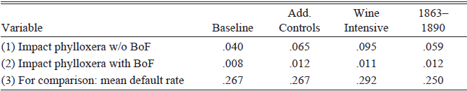
The results are therefore consistent with the view that eligibility for central bank operations to some extent prevented the agricultural crisis from spilling over to solvent but liquidity-constrained firms in the rest of the economy. To assess the magnitude of the effect, we look at the impact of the average phylloxera shock on the default rate by multiplying the coefficient on phylloxera by the average size of the phylloxera shock, as well as adding the value of the interaction terms at the respective mean values of the interacted variable. Table 5 gives the results for the four regression specifications in Table 4. For every specification, the table distinguishes two cases: the first row gives the effect of phylloxera on the default rate, assuming that the Bank of France is not present in the district (Elig it BoF = 0). The resulting numbers can then be compared with the general level of the default rate in the economy in the third row. Column (1) shows that, according to the simplest specification, the average phylloxera shock leads to an increase of 0.040 percentage points in the default rate relative to an average default rate of 0.267 percent, or about 15 percent. Adding additional controls in Column (2), the effect increases to a plus of 0.058 percentage points, or an increase of slightly above 24 percent in the district default rate. This confirms the economically significant impact of phylloxera, which seems reasonable given the importance of wine in the economic structure of France; see Figure 2. The result is basically unchanged when the sample is restricted to 1862–1890. When restricting the sample to the wine-intensive districts, the effect increases, which seems reasonable as well.
ESTIMATED EFFECTS OF PHYLLOXERA ON THE DEFAULT RATE

Table 5 Long description
The table presents data on the estimated effects of phylloxera on default rates, comparing baseline and additional controls across different time periods. It has three rows and four columns. The rows are labeled as Impact phylloxera without Bank of France, Impact phylloxera with Bank of France, and mean default rate for comparison. The columns are labeled as Baseline, Add Controls, and Wine Intensive 1863-1890. Row 1: Impact phylloxera without Bank of France, Baseline 0.040, Add Controls 0.065, Wine Intensive 1863-1890 0.095. Row 2: Impact phylloxera with Bank of France, Baseline 0.008, Add Controls 0.012, Wine Intensive 1863-1890 0.011. Row 3: mean default rate for comparison, Baseline 0.267, Add Controls 0.267, Wine Intensive 1863-1890 0.250. The table shows how phylloxera impacts default rates under different conditions and time frames.
Notes: The table shows the impact of the average phylloxera shock on the district default rates by multiplying the coefficients on phylloxera for the different regression specifications given in Table 3 with the average size of the phylloxera shock, as well as adding the value of the interaction terms at the respective mean values of the interacted variable. In line (1), the number of branches of the BoF is set to zero. In line (2), the number of branches of the BoF is set to the average number of branches in the sample, conditional on at least one branch being open.
Source: Authors’ calculations.
Moving on the second row, the same exercise is done assuming that the Bank of France was present. To account for the bank’s branches, Elig it BoF is set equal to its mean value conditional on at least one branch being present, and the interaction term with phylloxera is evaluated accordingly (the conditional mean number of branches is 1.20 for the full sample, 1.13 for the wine-intensive districts, and 1.08 for the restricted period 1863–1890). As can be seen across all specifications, given an average presence of the Bank of France, the effect of an average phylloxera shock is still positive (i.e., the default rate increases), but much smaller—roughly 4 percent, for instance, for wine-intensive districts. Note that this does not mean that phylloxera had a small effect; the direct consequences for agriculture were dramatic. However, this result confirms the hypothesis that the liquidity backstop offered by the Bank of France largely prevented the agricultural shock from spilling over to the secondary and tertiary sectors.
Next, we run several robustness checks, for which tables are reported in Online Appendix D. First, the results are similar when alternative measures of shock it are used. Table D2 gives the results when the economic effects of phylloxera are measured using impactdummy it; Table D3 when using spotted it. Again, the signs of all the relevant variables are unaffected, both in the most parsimonious specification in Column (1) and the specification including additional controls in Column (2). The main difference with the specification using impactvolume it and reported in Table 4 is that the coefficient on the shock measures, while correctly signed, is now sometimes not statistically significant. This result is not surprising given that both spotted it and impactdummy it are less precise measures for the impact of phylloxera than impactvolume it. Importantly for the argument on the role of the Bank of France in mitigating the negative effects of phylloxera, however, the interaction term is correctly signed and highly significant with both alternative shock measures.
A second robustness check restricts the sample to wine-intensive districts only. In all Tables 4, D2, and D3, Column (3) presents a specification excluding districts with below-average wine production. Wine-intensive districts are defined as districts where wine accounts for more than 15 percent of the total agricultural production. Again, the main results are unchanged. The coefficients in front of the shock variable and the interaction term do not change or increase slightly, and their level of significance remains unaffected or even increases somewhat.
In the next step, we look only at the years from the arrival of phylloxera in 1863 until the identification of a cure in 1890. With a drastic reduction in the number of observations, the coefficients reported in Column (4) of all tables are correctly signed, and the significance of the interacted term is maintained.
A last set of robustness checks concerns potential spatial correlation. The results of the estimation of Equation (2) are given in Table D4. We focus on the different eligibility and shock measures in the parsimonious specification and include additional controls only when estimating the baseline model with impactvolume it as the shock and branches as eligibility variables. The inclusion of a spatial error term does not change the magnitude and statistical significance of the coefficients. A comparison of the coefficients in Table D4 with those in the corresponding specifications without a spatial error term in Tables 4, D2, and D3 shows that most of the coefficients and standard errors remain completely unchanged. Spatial correlation has, thus, no bearing on the results presented.
CENTRAL BANK LENDING, MORAL HAZARD, AND THE ABSENCE OF A BAILOUT
We now show that the decrease in the default rates due to a higher number of Bank branch offices cannot be explained by a central bank bailout of insolvent borrowers. We have already seen that farmers had no access to the discount facility and that therefore moral hazard concerns do not apply. The situation could have potentially been different for industrial or service firms. Here, it is necessary to distinguish between a geographic extension of eligibility, offering more agents the possibility to obtain liquidity under given conditions, and a loosening of lending criteria, making borrowing easier for all agents who have access to the central bank.
The section on the “BRANCHING DECISIONS OF THE BANK OF FRANCE” has already discussed at length that the Bank of France did not expand the geographic reach of its network as a response to phylloxera. To see whether the Bank maintained or loosened its lending criteria during the pandemic, we construct a measure of the risk taken by the Bank in its discounting. To that end, we have collected the number of protested bills, where protested means that the bills were not paid when due. Figure 4 plots the percentage of the Bank’s portfolio and compares it to the percentage of protested bills at the economy-wide level. The proportion of bills unpaid at maturity in the Bank of France portfolio stands at 0.015 percent during the period between 1820 and 1913. This level was much lower than the ratio at the economy-wide level, which averaged 2.18 percent during the period from 1842 to 1912. Also, there is no correlation between the spread of phylloxera and the provisions for losses in the portfolio. If there is a trend over time, it is downward. Apparently, the Bank did not become more lenient over time.
This is no surprise given the monitoring of counterparty risks by the Bank of France. As the discount decision consists of the outright purchase of a bill of exchange, any default on payment at due date has a direct impact on the earnings and thus the dividend of the Bank. As a privately owned company traded on the Paris Stock Exchange, the Bank of France had a keen interest in screening the bills carefully in order to minimize its exposure to defaults. As a result, the Bank of France applied strict rules.
The strict rules described in Avaro and Bignon (Reference Avaro and Bignon2019) explain why the Bank suffered an order of magnitude less from non-payments than the average discounter in the economy (see Figure 4). Even then, the losses suffered by the Bank when discounting were much lower than the volume of protested bills in its portfolio. By putting his signature on the back of the bill, every endorser became liable to pay the bill at maturity if the drawee was in default.Footnote 17 The guarantee was easy and quite cheap to call on.Footnote 18 The percentage share of unpaid bills plotted in Figure 4 relates to the cases where a guarantee was called, not to the share of bills to be written off. While the procedure could take a couple of weeks, ultimately, almost all protested bills were paid by the guarantors, and losses were close to zero.
CONCLUSION
This article provides an empirical analysis of the beneficial effects of broad access to the central bank as a lender of last resort. Our goal is quantitative and aims to provide support for theories emphasizing the beneficial effects of credit-easing policies. Our analysis is based on a newly assembled dataset tracing the economic evolution of all French districts during the period from 1851 to 1913. We exploit a quasi-natural experiment that occurred in France in the nineteenth century.
To test for the consequences of access to central bank lending, we study a negative productivity shock triggered by an agricultural disease. In our set-up, the positive effect of the eligibility to the central bank discount window stems not primarily from actual lending but from agents’ understanding that they can turn to the Bank whenever liquidity falls short. The dampening effect of the central bank discount did not stem from lending to distressed agents on favorable terms. Rather, by discounting, the central bank liquefied the wealth of private agents, that is, transformed assets that could not be traded, or only at a high cost, into liquid banknotes that allowed borrowers to pay their bills.
Our paper, therefore, contributes to the policy debate on eligibility rules of central banks. We show that, when a crisis hits, eligibility must move center stage, as having access to the central bank and holding the required collateral can determine the survival of many firms. If there is any lesson to be drawn from this past experience in terms of today’s monetary policy, our results stress the importance of the framework in which the central bank implements its monetary policy in times of crisis.


 Open access