





1. Introduction
The use of porosity as an adaptation to traditional rigid impermeable aerofoils is a commonplace area of interest for minimising aerofoil–turbulence interaction noise (Geyer, Sarradj & Giesler Reference Geyer, Sarradj and Giesler2012; Roger, Schram & De Santana Reference Roger, Schram and De Santana2013; Ayton Reference Ayton2016; Chaitanya et al. Reference Chaitanya, Joseph, Chong, Priddin and Ayton2020). Both leading-edge noise, generated by upstream turbulence impinging on the aerofoil, and trailing-edge noise (also known as self-noise), generated by boundary layer turbulence scattering off the trailing edge can be reduced by replacing an impermeable aerofoil with a fully porous aerofoil (Geyer, Sarradj & Fritzsche Reference Geyer, Sarradj and Fritzsche2010), or partially porous aerofoil (Geyer & Sarradj Reference Geyer and Sarradj2019).
To date, these investigations, theoretical (Ayton Reference Ayton2016), numerical (Cavalieri, Wolf & Jaworski Reference Cavalieri, Wolf and Jaworski2016; Bae & Moon Reference Bae and Moon2011) and experimental (Geyer et al. Reference Geyer, Sarradj and Fritzsche2010; Geyer & Sarradj Reference Geyer and Sarradj2019), focus on using one uniform material to impose the porosity, with chordwise variations achieved only through the use of partially porous aerofoils wherein there is an unavoidable and instantaneous variation of the boundary from impermeable to permeable. At this junction, additional noise is generated by edge scattering (Rienstra & Peake Reference Rienstra and Peake2005; Ayton Reference Ayton2016). However, the benefit of a partially porous aerofoil is in its aerodynamics rather than its acoustics; fully porous aerofoils, whilst acoustically beneficial, have significant aerodynamic penalties (Geyer et al. Reference Geyer, Sarradj and Fritzsche2010); on the other hand, partially porous aerofoils have lessened aerodynamic penalties but produce more noise than fully porous aerofoils (Iosilevskii Reference Iosilevskii2011; Geyer & Sarradj Reference Geyer and Sarradj2019). The steady aerodynamics of partially porous aerofoils have previously been predicted theoretically by Iosilevskii (Reference Iosilevskii2011), which has been extended to aerofoils with porosity gradients by Hajian & Jaworski (Reference Hajian and Jaworski2017).
This paper, therefore, investigates the effect of porosity gradients on the noise generated by aerofoil–turbulence interaction. We also implement the Riemann–Hilbert solution of Hajian & Jaworski (Reference Hajian and Jaworski2017) to determine the lift coefficient, and thus a measure of the aerodynamic performance of the plates. In these models we allow an arbitrary variation in porosity along a finite perforated flat plate, modelling a thin permeable aerofoil.
The acoustic response will be achieved through a Mathieu collocation method (Colbrook & Priddin Reference Colbrook and Priddin2020). This method restricts us to solving for the acoustics in zero-lift configurations (zero angle of attack in uniform mean flow). The combined aeroacoustic and aerodynamic results will, therefore, indicate the qualitative trends of performance as we vary the porosity along the plate although, since the acoustics are restricted to the zero-lift configuration, they will not be quantitatively comparable.
Throughout this paper, we pay particular attention to monotonic porosity distributions as inspired by two species of birds: barn owls (tyto alba), known for their silent flight (Graham Reference Graham1934; Lilley Reference Lilley1998), and common buzzards (buteo buteo). We recreate these chordwise-varying porosity distributions in our flat-plate model as an initial study into the effects of porosity distributions on both aerofoil–turbulence interaction noise and potential lift, before considering more general monotonic distributions. Porosity is a known feature that promotes the silent flight of owls. Therefore, we expect the owl-like distribution to outperform the buzzard-like distribution acoustically, although we note there are many other features we do not consider in our model, such as serrations and canopies (Jaworski & Peake Reference Jaworski and Peake2020), which aid the owl's silent flight. We also note these two species have different flight speeds; the owl flies at speeds  $6\text {--}10\ \mathrm {ms}^{-1}$ (Neuhaus, Bretting & Schweizer Reference Neuhaus, Bretting and Schweizer1973) and the buzzard at a mean speed of $11.6\ \mathrm {ms}^{-1}$ (Alerstam et al. Reference Alerstam, Rosén, Bäckman, Ericson and Hellgren2007). Mean flow is accounted for in our model, but we apply a low Mach number approximation throughout which, particularly for trailing-edge noise, eliminates the difference in flight speed.
The layout of this paper is as follows. In § 2, we discuss the set-up of the acoustic mathematical model and the Mathieu collocation method for solving the acoustic problem. In § 3, we review the aerodynamic model from Hajian & Jaworski (Reference Hajian and Jaworski2017), which we shall use to calculate lift coefficients. In § 4, we discuss the measurements taken from birds’ wings and how we relate these to the mathematical model of porosity on a flat plate. In § 5, we present results and discuss general monotonic porosity variations. Finally, our conclusions are given in § 6.
2. Mathematical model for the acoustics
We consider an incident field impinging on a flat plate situated at  $-1\leq x\leq 1$ and $y=0$, where lengths have been non-dimensionalised by semi-chord. The plate is in uniform horizontal flow, with velocities non-dimensionalised by the far-upstream mean flow velocity. The incident field will have velocity potential denoted by $\phi _{{I}}$ and the scattered field by $\phi$. The incident pressure field is given by $p_{{I}}=-\rho _f({\textrm {D}\phi }/{\textrm {D}t})$, where $\rho _f$ is the mean fluid density and ${\textrm {D}\phi }/{\textrm {D}t}$ denotes the material derivative. Pressure shall henceforth be non-dimensionalised by $\rho _{f}c_{0}^{2}$ with $c_{0}$ denoting the speed of sound, so that throughout we deal with dimensionless fields $\phi _{{I}}$ and $\phi$.
We assume that  $\phi$ has the usual time dependence $\textrm {e}^{-\textrm {i}\omega t}$ (which will be omitted throughout), and hence for low Mach number flow, $\phi$ satisfies the Helmholtz equation
 \begin{equation} \left(\frac{\partial^2}{\partial x^2}+\frac{\partial^2}{\partial y^2} +k_0^2 \right) \phi=0 , \end{equation}
where  $k_0=\omega /c_0$ is the acoustic wavenumber for angular frequency $\omega$.
We apply an impedance boundary condition given by
 \begin{equation} \frac{\partial \phi}{\partial y}+\frac{\partial \phi_{I} }{\partial y} = \mu(x) \left(\phi_{u}-\phi_{l}\right)= \mu(x) [\phi](x), \end{equation}
to model the effects of the porous plate, where  $\mu =\alpha _{H}K_{R}/({\rm \pi} r^{2})$ is the porosity parameter (Howe, Scott & Sipcic Reference Howe, Scott and Sipcic1996; Jaworski & Peake Reference Jaworski and Peake2013). Here $K_{R}$ is the Rayleigh conductivity (Rayleigh Reference Rayleigh1945), which for evenly spaced circular apertures of radius $r$, is given by $K_{R}=2r$. The fractional open area is $\alpha _{H}$ (Howe Reference Howe1998). Such a model is valid for $\alpha _{H}^{2}\ll 1$, and $k_{0}r\ll 1$. We use the notation $\phi _{u}$ and $\phi _{l}$ to denote the values of the field just above and just below the plate respectively, and the jump in $\phi$ across the plate is denoted by $[\phi ]$. Finally, the scattered field is required to satisfy the Sommerfeld radiation condition for outgoing waves at infinity.
Note that, unlike previous theoretical models (Jaworski & Peake Reference Jaworski and Peake2013; Ayton Reference Ayton2016), we allow the porosity parameter  $\mu (x)$ to vary along the plate. This could be achieved in a number of practical ways; we could link its variation to a variation in $\alpha _{H}$, keeping $r$ and $K_{R}$ constant along the plate. Thus the number of apertures in the plate per unit area varies along the chord, but the size of the apertures remains constant. An identical porosity distribution, i.e. an identical variable $\mu (x)$, could alternatively be achieved through variation of the aperture radius, or a combination of both varying radius and open area. Any such variation presents itself in our model as a fundamental variation in acoustic impedance, governed by the single parameter $\mu (x)$. A specification of how one practically implements the variation of impedance is not required. Nevertheless, throughout this paper, for simplicity, we shall describe the porosity (impedance) distribution as arising due to variation of aperture spacing, $\alpha _{H}$, rather than a full variation of $\alpha _{H}K_{R}/r^{2}$. This, therefore, provides immediate instruction as to how one would practically manufacture a plate corresponding to our model for testing. It may be helpful to the reader to consider our variation of porosity through a change in hole spacing as similar to the variation of acoustic impedance in traditional liners through a change of resonator depth (Jones et al. Reference Jones, Nark, Watson and Howerton2017). We note, however, this choice may lead to unphysical values of $\alpha _{H}>1$ and in such a case, to design a corresponding practical experiment, variations of $r$ and $K_{R}$ would be necessary to achieve the same $\mu (x)$ values. We stress, it is only the overall porosity (impedance) variation of $\mu (x)$ that truly matters in this model, and, as a whole parameter, this always permits a physically relevant perforated surface. Our set-up is illustrated in figure 1.
Schematic of the variable-porosity plate with edges at  $x=-1$ and $x=1$. The plate extends infinitely in the spanwise ( $z$) direction.

2.1. Mathieu function expansion
Here, we now solve the problem using the Mathieu function collocation method of Colbrook & Priddin (Reference Colbrook and Priddin2020) which provides an expansion of  $\phi$ in Mathieu functions using separation of variables in elliptic coordinates. A full discussion of this method can be found in Colbrook & Priddin (Reference Colbrook and Priddin2020), and user-friendly code for the method can be found at https://github.com/MColbrook/MathieuFunctionCollocation.
When using elliptic coordinates,  $x=\cosh (\nu )\cos (\tau ),y=\sinh (\nu )\sin (\tau )$, the appropriate domain becomes $\nu \geq 0$ and $\tau \in [0,{\rm \pi} ]$. The Helmholtz equation with homogeneous Dirichlet boundary condition (the continuity condition) along $\{(x,y):y=0,|x|>1\}$ and the Sommerfeld condition at infinity become
 \begin{equation} \left.\begin{gathered} \frac{\partial^2{\phi}}{\partial \tau^2}+\frac{\partial^2{\phi}}{\partial \nu^2}+\frac{\cosh(2\nu)-\cos(2\tau)}{2}k_0^2{\phi}=0,\\ \phi|_{\tau=0}=\phi|_{\tau={\rm \pi}}\equiv 0,\\ \lim_{\nu\rightarrow\infty}\nu^{1/2}\left(\frac{\partial}{\partial\nu}-\textrm{i} k_0\right){\phi}(\nu,\tau)=0. \end{gathered}\right\} \end{equation}
This set of equations does not currently impose the porosity (impedance) condition along the plate and so provides a general solution for any boundary condition on the plate. We shall discuss the application of our particular boundary condition shortly in § 2.2. To simplify the formulae, we let  $\kappa =k_0^2/4$. Separation of variables for solutions of the form $V(\nu )W(\tau )$ leads to the regular Sturm–Liouville eigenvalue problem
 \begin{equation} \left.\begin{gathered} W''(\tau)+\left(\lambda-2\kappa\cos(2\tau)\right)W(\tau)=0,\\ W(0)=W({\rm \pi})=0. \end{gathered}\right\} \end{equation}
The solutions of this are sine-elliptic functions, denoted by  $\mathrm {se}_n$ with eigenvalue $\lambda _n$, which we expand in a sine series as
 \begin{equation} \mathrm{se}_n(\kappa;\tau)=\mathrm{se}_n(\tau)=\sum_{l=1}^\infty B_{l}^{(n)}\sin(l\tau). \end{equation}
This series converges absolutely and uniformly on all compact sets of the complex plane (Olver et al. Reference Olver, Lozier, Boisvert and Clark2010). The eigenfunctions are orthogonal, and we choose the normalisation
 \begin{equation} \int_0^{\rm \pi} \mathrm{se}_m(\tau)\mathrm{se}_n(\tau)\,\textrm{d}\tau=\frac{\rm \pi}{2}\delta_{mn}. \end{equation}
We find the coefficients  $B_l^{n}$ via a simple Galerkin method. The corresponding $V(\nu )$ with the appropriate radiation condition at infinity are given by the Mathieu–Hankel functions
 \[ \mathrm{Hse}_{n}(\kappa;\nu)=\mathrm{Hse}_{n}(\nu)=\mathrm{Jse}_{n}(\nu)+\textrm{i} \mathrm{Yse}_{n}(\nu). \]
These Mathieu–Hankel functions can be expanded in a series using Bessel functions (McLachlan Reference McLachlan1964; Olver et al. Reference Olver, Lozier, Boisvert and Clark2010)
 \begin{equation} \mathrm{Hse}_{n}(\nu)=\sum_{l=1}^\infty\frac{(-1)^{l+n}B_l^{(n)}}{C_n}\left[{J}_{l-1}(\textrm{e}^{-\nu}\sqrt{\kappa}){H}_{l+p_n}^{(1)}(\textrm{e}^{\nu}\sqrt{\kappa})- {J}_{l+p_n}(\textrm{e}^{-\nu}\sqrt{\kappa}){H}_{l-1}^{(1)}(\textrm{e}^{\nu}\sqrt{\kappa})\right], \end{equation}
where  $p_n=(1+(-1)^n)/2$. Here, $J_n$ denotes the Bessel function of the first kind of order $n$ and $H_n^{(1)}$ denotes the Hankel function of the first kind of order $n$. The series in (2.7) converges absolutely and uniformly on all compact sets of the complex plane (Olver et al. Reference Olver, Lozier, Boisvert and Clark2010). We choose the normalisation constants $C_n$ so that $\mathrm {Hse}_{n}'(0)=1$.
The full general solution can then be written as
 \begin{equation} {\phi}(\nu,\tau)=\sum_{n=1}^\infty a_n \mathrm{se}_{n}(\tau)\mathrm{Hse}_{n}(\nu), \end{equation}
where  $a_{n}$ are unknown coefficients. These coefficients are determined by applying the appropriate boundary condition along the plate, which we do so in § 2.2.
Given the Bessel function expansion of  $\mathrm {Hse}_{n}(\nu )$ in (2.7), we can directly compute the far-field directivity $D(\theta )$ from (2.8) using asymptotics of Bessel functions. In the appropriate limit, $\tau$ becomes the polar angle $\theta$, whereas $\nu$ becomes $\cosh ^{-1}(r)$ (where $(r,\theta )$ denote the usual polar coordinates). This leads to
 \begin{equation} D(\theta)=\sqrt{\frac{2}{{\rm \pi} k_0}}\sum_{n=1}^\infty \frac{a_nB_1^{(n)}}{C_n} \exp\left(\frac{(2p_n-3){\rm \pi}}{4}\textrm{i}\right)\mathrm{se}_{n}(\theta). \end{equation}
An advantage of our approach is that we implicitly compute a sine series for the far-field directivity  $D(\theta )$ through the sine-elliptic functions $\mathrm {se}_{n}(\theta )$ given by (2.5).
Finally, we define the total far-field noise, measured in dB, as
 \begin{equation} P = 10\log_{10}\left(\int_{0}^{\rm \pi}|D(\theta)|^{2}\,\textrm{d}\theta\right), \end{equation}
which may be computed numerically from the series expansion for  $D(\theta )$.
2.2. Employing the boundary conditions
Here, we now determine the unknown coefficients  $a_{n}$ in the expansion (2.8), as required for our particular boundary condition (2.2). We do so by adopting a spectral collocation method to calculate their approximate value. Throughout, we denote the approximate coefficients by $\tilde a_n$.
We take our general solution (2.8) and substitute into (2.2), written in original  $(x,y)$ coordinates. We truncate the expansion at $N$ terms to obtain the approximate condition
 \begin{equation} \sum_{n=1}^N \tilde a_n \mathrm{se}_{n}\left(\cos^{-1}\left({x}\right)\right)\left[1-2\,\mathrm{Hse}_{n}(0) \mu(x)\sqrt{1-x^2}\right]=-\sqrt{1-x^2}\cdot\frac{\partial \phi_{{I}} }{\partial y}(x). \end{equation}
We now evaluate this at chosen collocation points,
 \begin{equation} x=\cos\left(\frac{2j-1}{2N}{\rm \pi}\right),\quad j=1,\ldots,N, \end{equation}
which correspond to Chebyshev points in Cartesian coordinates and equally spaced points in elliptic coordinates (Trefethen Reference Trefethen2000; Boyd Reference Boyd2001). This gives rise to an  $N\times N$ linear system for the unknown coefficients $\{\tilde a_n\}_{n=1}^N$, which we precondition by rescaling to ensure that each row of the resulting matrix has a constant $l^1$ vector norm.
2.3. Avoiding numerical cancellations
The terms in the series (2.7) can easily be evaluated for small  $l$. However, for large $l$, the terms in the series suffer from underflow and overflow associated with cancellations between the Bessel and Hankel functions. For large $l$ and fixed $x\in \mathbb {R}_{>0}$ we use the asymptotics
 \begin{equation} \left.\begin{gathered} {J}_{l}(x)= \sum_{j=0}^m\frac{(-1)^j}{j!(\,j+l)!}\left(\frac{x}{2}\right)^{2j+l}+{O}\left(\frac{1}{(m+l+1)!}\right),\\ {H}_{l}^{(1)}(x)=\frac{-\textrm{i}}{\rm \pi}\left(\frac{2}{x}\right)^{l}\sum_{j=0}^m\frac{(l-j-1)!}{j!}\left(\frac{x}{2}\right)^{2j}+{O}\left((l-(m+2))!\right), \end{gathered}\right\} \end{equation}
valid as  $l\rightarrow \infty$. For fixed $a,b\in \mathbb {Z}$, this gives the asymptotic form
 \begin{align} &{J}_{l+a}(\textrm{e}^{-\nu}\sqrt{\kappa}){H}_{l+b}^{(1)}(\textrm{e}^{\nu}\sqrt{\kappa})\nonumber\\ &\quad=\frac{-\textrm{i}}{\rm \pi}\left(\frac{\sqrt{\kappa}}{2}\right)^{a-b}\exp({-\nu(2l+a+b)})\left[{\sum_{j=0}^m\frac{(-1)^j(l+a)!}{j!(\,j+l+a)!}\left(\frac{\textrm{e}^{-\nu}\sqrt{\kappa}}{2}\right)^{2j}}\right]\nonumber\\ &\qquad\times\left[\sum_{j=0}^m\frac{(l+b-j-1)!}{j!(l+a)!}\left(\frac{\textrm{e}^{\nu}\sqrt{\kappa}}{2}\right)^{2j}\right]+{O}\left(l^{-(m+2)}\right). \end{align}
 We found this to be an excellent approximation for large  $l$. It can also be accurately evaluated for moderate $m$ since the terms $(l+a)!/(\,j+l+a)!$ and $(l+b-j-1)!/(l+a)!$ can be evaluated as products of $j$ and $|\,j+1+a-b|$ terms respectively. In what follows, we typically used this asymptotic form when $l>100$ and took up to $m=5$ terms. When plotting errors of our method, we were careful to compare against converged computations for which the series (2.7) was evaluated directly using extended precision (such checks were the only place where we made use of extended precision).
3. Theoretical calculation of lift
Here, we briefly review the theory of Hajian & Jaworski (Reference Hajian and Jaworski2017) to calculate the lift coefficient of a porous plate, where the porosity is permitted to vary along the chord. Note, this does not account for the full aerodynamics since we are not calculating drag.
We suppose a flat-plate aerofoil is placed in uniform upstream flow of speed  $U_{inf}{\boldsymbol {e}}_{x}$, where ${\boldsymbol {e}}_{x}$ denotes the horizontal direction. We let $z_{a}(x)$ denote the camber line of the plate, which for our case of a flat plate at fixed angle of attack $\alpha$ ensures $\textrm {d}z_{a}/\textrm {d}x = -\alpha$. Under the assumption of small disturbance (neglecting $O(\alpha ^{2})$), the plate lies in the region $-1\leq x\leq 1$ where, once again, lengths are non-dimensionalised by semi-chord.
Assuming a Darcy-type boundary condition, we may connect the pressure jump to the local normal flow rate through the plate,  $w_{s}$:
 \begin{equation} w_{s}=-C \mathcal{R}(x) (p_{u}-p_{l}), \end{equation}
where  $C$ is defined as a porosity coefficient, and $\mathcal {R}(x)=\alpha _{H}(x)$ is the porosity distribution (Hajian & Jaworski Reference Hajian and Jaworski2017, (2.9)). The integral equation linking the pressure jump to the camber line and porosity distribution in thence given by
 \begin{equation} \rho_{f}U_{inf}C\mathcal{R}(x)p(x)-\frac{1}{2}\int\kern-10pt ---_{-1}^{1}\frac{p(t)}{t-x}\,\textrm{d}t = 2\frac{\textrm{d}z_{a}}{\textrm{d}x}, \end{equation}
where pressure is non-dimensionalised by  $(\rho _{f}U_{inf}^2)/{2}$. (Note this is different to the non-dimensionalisation for the acoustics where pressure is non-dimensionalised with respect to speed of sound). This equation is solved to yield
 \begin{align} p(x)&=\frac{4\psi(x)}{1+\psi^{2}(x)}\frac{\textrm{d}z_{a}}{\textrm{d}x}- \frac{4}{{\rm \pi} \sqrt{1+\psi^{2}(x)}}\exp\left({\int\kern-10pt ---_{-1}^{1}\frac{k(\psi(t))}{t-x}\,\textrm{d}t}\right) \nonumber\\ &\quad \times \int\kern-10pt ---_{-1}^{1}\frac{\textrm{d}z_{a}/\textrm{d}t}{\sqrt{1+\psi^{2}(t)} \exp\left(\displaystyle{\int\kern-10pt ---_{-1}^{1}\dfrac{k(\psi(\xi))}{\xi-t}\,\textrm{d}\xi}\right)(x-t)}\,\textrm{d}t, \end{align}
where  $\psi (x)=2\rho _{f}U_{inf}C\mathcal {R}(x)$, and $k(y)={\rm \pi} ^{-1}\cot ^{-1}(y)$. Implementation and validation by comparison with Hajian & Jaworski (Reference Hajian and Jaworski2017) is discussed shortly.
4. Flow resistivity through wings
To provide an initial porosity distribution along a flat plate, we consider the distributions that appear in nature, in particular for barn owns and common buzzards.
4.1. Experimental measurements
In order to obtain quantitative data on the permeability of owl wings compared to the wings of other, non-silently flying birds of prey, measurements of the flow resistance were conducted on a set of prepared wing specimen. For measurements on porous materials according to ISO 9053 (1991), the materials have to be cut into cylindrical samples of constant thickness and tightly fitted into a sample holder. Since that is obviously not possible for prepared bird wings, which may consist of only a single layer of feathers especially close to the trailing edge (see, for example, the work of Nachtigall & Klimbingat (Reference Nachtigall and Klimbingat1985) and Bachmann, Mühlenbruch & Wagner (Reference Bachmann, Mühlenbruch and Wagner2011)), a special measurement head was constructed. It can be pressed onto the surface of the wings with a defined force, allowing one to seal off the area of contact between the planar measuring head and the feather surface. With the help of this measurement head, a defined air flow with a volumetric airflow rate  $q$ (in $\textrm {m}^3\,\textrm {s}^{-1}$) is conducted through the prepared wing (see figure 2). The air flow resistance $R$ at this position of the wing is then calculated from the resulting static pressure difference across the wing
 \begin{equation} R = \frac{p_u - p_l}{q}. \end{equation}
Set-up used to measure the wing air flow resistance  $R$ (4.1).

Such measurements were conducted at each chosen wing location for seven different volume flows. According to ISO 9053 (1991), the resulting value of the air flow resistance was then obtained by linear extrapolation of the results to a low flow speed of  ${5 \times 10^{-4}\ \mathrm {ms}^{-1}}$.
4.2. Theoretical modelling
We must relate the experimentally recovered values of flow resistance,  $R$, to both the aeroacoustic porosity parameter $\mu$, and the aerodynamic parameter, $C$. We begin with the aeroacoustic parameter $\mu$. Recall that $\mu (x)=\alpha _{H}(x)K_{R}/({\rm \pi} r^{2})$, where we assume the porosity is created by circular apertures of constant radius, $r$, and, for a plate with circular apertures, the Rayleigh conductivity of the plate, $K_{R}=2r$. However, for an arbitrary material, $K_{R}$ is defined as $K_{R}=Q/(\phi _{u}-\phi _{l})$, where $Q=\textrm {d}q/\textrm {d}t$ is the volume flux through the plate. Hence for the wing in harmonic flow, $K_{R}=\omega ^{2} \rho _{f}/R$. We thus have two ways of calculating $\mu (x)$
 \begin{equation} \mu(x) = \alpha_{H}(x)\frac{2}{{\rm \pi} r}, \quad \mu_{{\textit{exp}}}(x) = \alpha^{{\textit{exp}}}_{H} \omega^{2} \rho_{f}\frac{1}{R}\frac{1}{{\rm \pi} r_{{\textit{exp}}}^{2}}, \end{equation}
where  $\alpha _{H}$ denotes the open area ratio of circular apertures or radius $r$ in a flat plate, $\alpha ^{{exp}}_{H}$ denotes the open area ratio of pores of typical radius $r_{{exp}}$ in a wing, and $R$ is the measured flow air flow resistance. We may thus equate the two to provide values for $\alpha _{H}(x)$ to input into our model
 \begin{equation} \alpha_H(x)=\frac{\omega^{2}\rho_{f}r\alpha_{H}^{{exp}}}{2Rr_{{exp}}^{2}}. \end{equation}
We shall assume that the chordwise variation in (4.3) arises only due to the air flow resistance,  $R$, and that $\alpha _{H}^{{exp}}$ and $r_{{exp}}$ are constant. According to Jaworski & Peake (Reference Jaworski and Peake2013) we take the value $\alpha _{H}^{{exp}}=0.0014$. This value arises from the trailing-edge brush experiment of Herr (Reference Herr2007) wherein polypropylene fibres with physical properties similar to the feather keratin of owl wings are used to investigate noise reduction. The fibres which exhibited the best noise reduction were converted to the equivalent open area ratio parameter of $\alpha _{H}^{{exp}}=0.0014$ by Jaworski & Peake (Reference Jaworski and Peake2013). Since in Jaworski & Peake (Reference Jaworski and Peake2013) lengths are non-dimensionalised by a bending wave number (which does not feature in our analysis since our plate is not flexible), it is more difficult to determine the corresponding value of $r_{{exp}}$. We, therefore, turn to detailed measurements made on the wings of barn owls by Bachmann, Wagner & Tropea (Reference Bachmann, Wagner and Tropea2012), which results in a value of $r_{{exp}}=5.5\times 10^{-4}\ \mathrm {m}$. This arises from supposing for a given barn owl feather there are two fringes per mm (Bachmann et al. Reference Bachmann, Wagner and Tropea2012) (and thus two gaps between the fringes per mm) and the total length of the vane of the feather is between $12.5$ and $15$ cm (Bachmann, Klän & Baumgartner Reference Bachmann, Klän, Baumgartner, Klass, Schroder and Wagner2007). Therefore each feather has between $250$ and $300$ apertures in the chordwise direction. We select $r_{{exp}}$ as the mid-value, supposing each aperture is $1/275$ of our fixed $15$ cm chord.
For the theoretical model, we shall suppose a manufactured flat plate has holes with radius  $r=1\ \mathrm {mm}$, which is practical to construct, and we use a typical frequency of $\omega =500\ \textrm {Hz}$ to complete our relationship between $R$ and $\alpha _{H}(x)$ since we wish to focus on low-frequency noise reductions. Assuming the area of measurement over the wing was $1\ \mathrm {cm}^{2}$, we obtain a value of $C=0.016$ for the porosity coefficient required in the lift calculations. We shall use the same value of the parameter group $\alpha _{H}^{{exp}}/({\rm \pi} r_{{exp}}^{2})$ (which can be viewed as the closed area of the wing) for the owl and buzzard as input to obtain our model, $\alpha _{H}(x)$. Whilst this is unlikely to be true for the buzzard, it provides an upper bound on the value of $\alpha _{H}$ to input to our model, as it is clear from detailed wing pictures (Chen et al. Reference Chen, Liu, Liao, Yang, Ren, Yang and Chen2012) that the closed area of the buzzard's wing is greater than that for the owl.
5. Results
5.1. Bio-inspired distributions
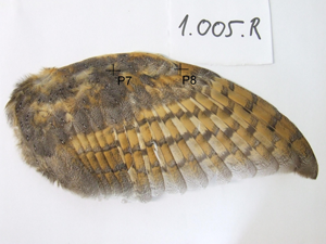
In this section, the results from the air flow resistance measurements on the prepared wings are summarised and converted to their corresponding  $\alpha _{H}$ values. Overall, five wings of the barn owl (tyto alba) and nine wings of the common buzzard (buteo buteo) were investigated to obtain the data used in the present study. For each wing, measurements were made at up to eight different positions, from which the first four were located in the region of the primary and secondary remiges, and hence closer to the trailing edge, while the last four were located closer to the leading edge, on the primary and secondary coverts. Figure 3 illustrates the locations at which samples were taken for Wing 3 of the barn owl. Table 1 summarises the results for the barn owl wings and table 2 those of the buzzard wings.
Upper and lower side of Wing 3 of the barn owl samples, showing the positions at which air flow resistance was measured.

Air flow resistance of the barn owl wings.

Air flow resistance of the buzzard wings.

We plot the variation in  $\alpha _{H}$ along the chord of each wing in figure 4, as calculated from experimental measurements and using (4.3). For microphones close to the wing tips (typically microphone position P1 as seen in figure 3), where the chord length is substantially different to the main wing, we have neglected those results, since our two-dimensional model cannot capture any spanwise variation in either wing shape or morphology. The chord length is measured from the photographic microphone locations using Matlab's image viewer app, as illustrated in figure 5. There is an outlier in the porosity data from the owl at a chord of ${\sim }60\,\%$. This outlier is due to the fact that these wings are biological systems and as such, not perfectly homogeneous. As mentioned before, this is especially true close to the trailing edge, where the wings consist only of one or two layers of feathers.
Porosity,  $\alpha _{H}$, as calculated from (4.3) from the measurement data for owls (blue, circles) and buzzards (black, crosses). Best fit curves are given according to Matlab's fit command.

Chord locations are measured from photographs using Matlab's image viewer app. Lengths are given in terms of the number of pixels.

Lines of best fit are produced using Matlab's fit command; both polynomial and exponential fitting were considered, and the best-fitting lines from each reproduced in figure 4. From these we shall take the variation which appears most likely in the owl wing to be
 \begin{equation} \alpha_{H}^{{owl}}=0.037+0.48\left(\frac{x}{2}+\frac{1}{2}\right), \end{equation}
and for the buzzard
 \begin{equation} \alpha_{H}^{{buzz}}=0.22\left(\frac{x}{2}+\frac{1}{2}\right)^{0.48}, \end{equation}
recalling that our chord lies in the region  $x\in [-1,1]$.
5.2. Numerical convergence and validation of methods
5.2.1. Acoustic calculations
To demonstrate convergence for the acoustic solution, in figure 6 we have plotted the relative errors against  $N$ (the number of basis functions used) for the values of $\alpha _H^{{owl}}$ and $\alpha _H^{{buzz}}$. These errors were estimated by comparing with values computed for larger $N$. We have plotted the relative error in the $L^2$ norm of $[\phi ]$ (the jump in the field across the plate) and the $P$ values for a quadrupole source. This shows convergence for a wide range of frequencies and also shows that we can easily gain several digits of relative accuracy.
Relative errors for  $[\phi ]$ (a, $L^2$ norm error over $[-1,1]$) and SPL (b). The method has a high order of algebraic convergence, allowing us to compute physical values to several significant figures.

To validate the acoustic calculations, we recreate figure 7(b) from Cavalieri et al. (Reference Cavalieri, Wolf and Jaworski2016) for a uniformly porous plate in figure 7, which shows excellent agreement. Note, our non-dimensionalisation of length is by semi-chord, whereas Cavalieri et al. (Reference Cavalieri, Wolf and Jaworski2016) use chord, therefore the values of  $k_{0}$ and $\alpha _{H}/R$ which we use are half the values from Cavalieri et al. (Reference Cavalieri, Wolf and Jaworski2016). For this figure, we place a quadrupole at $(1,0.008)$, corresponding to the non-dimensional location of $(1,0.004)$ used by Cavalieri et al. (Reference Cavalieri, Wolf and Jaworski2016).
Directivity,  $|D(\theta )|$, for $k_{0}=5$ for uniformly porous plates. This shows excellent agreement with figure 7(b) from Cavalieri et al. (Reference Cavalieri, Wolf and Jaworski2016).

5.2.2. Aerodynamic calculations
We recall that the pressure jump is given by (3.3), and the (non-dimensionalised) lift is then given by the integral
 \begin{equation} L=-\int_{-1}^1p(x)\,\textrm{d}x, \end{equation}
where the minus sign corresponds to the pressure jump being taken to be  $p_u-p_l$. To calculate this, we need an accurate and efficient method to compute iterates of the Hilbert transform. We used two approaches, which enables us to estimate the accuracy of our estimate through comparison. To ease the exposition, we only discuss the computation of the integral
 \begin{equation} g(x)=\int\kern-10pt ---_{-1}^{1}\frac{f(t)}{t-x}\,\textrm{d}t, \end{equation}
for  $x\in (-1,1)$ and sufficiently regular $f$ (e.g. integrable and locally Hölder continuous in $(0,1)$).
For the first method, we use a standard subtraction technique and consider the function
 \begin{equation} h(x,t):=\frac{f(t)-f(x)}{t-x}. \end{equation}
We use the fact that, for sufficiently regular  $f$ and for $x\in (-1,1)$, $h(x,t)$ is integrable over $t\in [-1,1]$ with
 \begin{equation} g(x)=\int_{-1}^1h(x,t)\,\textrm{d}t+f(x)\log\left(\frac{1-x}{1+x}\right). \end{equation}
We compute the integral of  $h$ using global adaptive quadrature through MATLAB's integral command, keeping track of the tolerances when iterating the procedure.
Our second approach is to make use of spectral methods based on Chebyshev polynomials, conveniently handled via the Chebfun software package (Driscoll, Hale & Trefethen Reference Driscoll, Hale and Trefethen2014). We first expand the function  $f(t)\sqrt {1-t^2}$ in Chebyshev polynomials of the first kind, $T_n(\cdot )$. These have the useful property that
 \begin{equation} \int\kern-10pt ---_{-1}^{1}\frac{T_n(t)}{(t-x)\sqrt{1-t^2}}\,\textrm{d}t={\rm \pi} U_{n-1}(x), \end{equation}
where  $U_n(\cdot )$ denote Chebyshev polynomials of the second kind (see (18.17.42) of Olver et al. Reference Olver, Lozier, Boisvert and Clark2010). We can thus compute an expansion of $g$ in Chebyshev polynomials of the second kind. We can iterate this procedure, taking advantage of rapid algorithms for computing the Chebyshev coefficients of $g(x)\sqrt {1-x^2}$ given the expansion of $g$.
$g$.
To verify our approach, we reproduce the results of Hajian & Jaworski (Reference Hajian and Jaworski2017), where
 \begin{equation} \psi(x)=\frac{5}{2}\left(1+\tanh\left(\nu_1\left(x+\frac{1}{2}\right)\right)\right),\quad \frac{\textrm{d}z_{a}}{\textrm{d}x}=\nu_2, \end{equation}
for constants  $\nu _1,\nu _2$. Figure 8 shows the results for $\nu _1=10$ and $\nu _1=1000$, with excellent agreement with figure 2 of Hajian & Jaworski (Reference Hajian and Jaworski2017).
Pressure distribution for  $\nu _1=10$ and $\nu _1=1000$, showing excellent agreement with the results of Hajian & Jaworski (Reference Hajian and Jaworski2017).

5.3. Bio-inspired results
Having validated our numerical methodology and shown results in agreement with previous work, we now present the acoustic results for the bio-inspired spanwise variations. In figure 9 we show the difference in far-field noise,  ${\rm \Delta} P=P^{{owl}}-P^{{buzz}}$ for $P$ defined by (2.10), generated for a near-field quadrupole source located at $(x_0,y_0)$ which models a turbulent trailing-edge source. The incident potential is therefore given by
 \begin{equation} \phi_{{I}} = \frac{\textrm{i} k_{0}^{2}}{4 r_{0}^{2}}(x-x_{0})(y-y_{0})H_{2}^{(1)}(k_{0}r_{0}), \end{equation}
where  $r_{0}=\sqrt {(x-x_0)^2+(y-y_0)^2}$, and $H_{n}^{(1)}$ are Hankel functions of the first kind.
Value of  ${\rm \Delta} P$ for a near-field quadrupole source at $x_{0}=0.95$ and various $y_{0}$. Negative values indicate the owl is quieter than the buzzard by that many dB.

It is perhaps no surprise to see that, via this model, the owl is predicted to produce less trailing-edge noise than the buzzard given that the trailing edge of the owl's wing is far more porous (has a higher  $\alpha _{H}$ value) than that of the buzzard's. This is particularly true for low frequencies which are known to be significantly reduced by porosity (Jaworski & Peake Reference Jaworski and Peake2013), however, the total level of low-frequency noise reduction is intrinsically linked to the vertical location of the quadrupole source. At higher frequencies, the owl is predicted to produce only $7$ dB less trailing-edge noise, and this is similar across all quadrupole locations. We cannot currently extend this analysis to frequencies much higher than $k_{0}=O(10)$ since outside of this range the asymptotic requirements for the homogenised boundary condition may not hold (Howe Reference Howe1998).
We first compare our theoretical model to the noise reduction achieved by uniformly porous aerofoils in Geyer & Sarradj (Reference Geyer and Sarradj2014, figure 8, lowest panel); there a low-frequency noise reduction of up to  ${\sim }10$ dB is reported for a porous aerofoil with low resistivity (high porosity) versus a porous aerofoil with high resistivity (low porosity). As frequency increases, the noise reduction diminishes, and in some cases, a noise increase is observed (largely due to surface roughness). This is in broad agreement with our theoretical results comparing the owl (low resistivity at the trailing edge) to the buzzard (comparatively higher resistivity at the trailing edge), although it does not account for any features of continuously varying porosity.
Next, we compare our predicted noise reduction to that measured experimentally for owl and buzzard wings in Geyer, Sarradj & Fritzsche (Reference Geyer, Sarradj and Fritzsche2013), and Sarradj, Fritzsche & Geyer (Reference Sarradj, Fritzsche and Geyer2010). The measurements from Geyer et al. (Reference Geyer, Sarradj and Fritzsche2013) were performed in an anechoic wind tunnel using microphone array techniques and acoustic beamforming (the same set-up as used in Geyer & Sarradj (Reference Geyer and Sarradj2014) for the uniformly porous aerofoils). As an example, figure 10 shows a schematic of the experimental set-up used by Geyer et al. (Reference Geyer, Sarradj and Fritzsche2013) as well as the sound pressure level difference between the results obtained for a buzzard wing and a barn owl wing of similar size (wings numbers 2 and 10 from Geyer et al. Reference Geyer, Sarradj and Fritzsche2013). For low to moderate frequencies, the measured noise reduction is between  $4$ and $12$ dB, whilst for higher frequencies, the noise reduction can exceed $20$ dB. In the flyover measurements on living birds (Sarradj et al. Reference Sarradj, Fritzsche and Geyer2010), however, smaller noise reductions between 3 dB at medium frequencies (around 1.6 kHz, $k_{0}\approx 2$) to 8 dB at higher frequencies (6.3 kHz, $k_{0}\approx 8.5$) have been obtained for the gliding flight noise from a barn owl compared to that from a Harris's hawk and a common kestrel (Sarradj et al. Reference Sarradj, Fritzsche and Geyer2010).
Schematic of the experimental set-up (a) and resulting  ${\rm \Delta} {SPL}$ between a buzzard wing and a barn owl wing at a flow speed of approximately $13\ \mathrm {ms}^{-1}$ (b) Geyer et al. (Reference Geyer, Sarradj and Fritzsche2013). Negative values indicate the owl is quieter than the buzzard by that many dB.

These results differ greatly from the porous aerofoil results in Geyer & Sarradj (Reference Geyer and Sarradj2014), particularly at high frequencies since there are numerous other silent-flight designs on the owl's wing which are not modelled by porosity alone, such as leading-edge combs, serrations and canopies, all of which may alter the owl's noise reduction at different frequencies (Jaworski & Peake Reference Jaworski and Peake2020). At high frequencies, serrations are particularly effective for noise reduction, with Moreau & Doolan (Reference Moreau and Doolan2013) observing up to  $13$ dB of noise reduction. Thus we anticipate the divergence of the theoretical predictions and the experimental results to be at least in part due to the serrated feature of the owl's wing. In addition, acoustic absorption by the owl's downy coat may play a role at high frequencies.
For comparison to owl wing noise, we therefore only concern ourselves with the low-to-moderate-frequency behaviour. Our theory overpredicts the noise reduction versus the realistic wing experimental measurements by up to  $7$ dB. This discrepancy at low frequencies may be due to the distortion of the flow over the wings (the three-dimensional behaviour) which has a significant effect on owl-generated noise since their leading-edge comb deflects the surface flow towards the wing tips. Geometric features such as the specific camber and thickness of the wing may also play a role. These features, which are lacking in our model, are also not taken account of in the porous aerofoil noise measurements in Geyer & Sarradj (Reference Geyer and Sarradj2014), which similarly disagree with the realistic wing measurements. We, therefore, believe our results correctly predict the effects of porosity along on aerofoil noise, but cannot represent the true total noise reduction of realistic wings due to a number of additional noise-reduction features present on realistic owl wings.
In figure 11 we consider the effects of the owl versus buzzard distributions on leading-edge noise, and see surprisingly that the owl distribution also would produce less leading-edge noise despite the two wings having similar leading-edge porosity values. We consider an incident gust by selecting a potential satisfying  $\partial \phi _{{I}}/\partial {y}|_{y=0} = -\textrm {e}^{\textrm {i}\delta x}$, where $\delta = k_{1}/\sqrt {1-M^{2}}$, and $k_{1}=\sqrt {1-M^{2}}k_{0}/M$ thus the Helmholtz number, $k_{0}$, is $\delta M$, such that the gust convects from upstream with the mean flow with Mach number $M$. Full details of why this is the case may be found readily in the literature for leading-edge noise (Tsai Reference Tsai1992; Ayton & Kim Reference Ayton and Kim2018). We assume the same impedance style boundary condition, (2.2), noting that here the low Mach number approximation has been used. The difference in leading-edge noise levels is given in figure 11, for $M=0.05$. We notice that, again, the owl is quieter than the buzzard for low frequencies, however, now the reduction is only approximately $3.5$ dB. Note the frequency range difference between the trailing-edge noise and the leading-edge noise; trailing-edge noise is a high-frequency phenomenon, whilst leading-edge noise is more dominant at lower frequencies. The lowest-frequency flyover noise reductions (Sarradj et al. Reference Sarradj, Fritzsche and Geyer2010) of $3$ dB are in agreement with our leading-edge noise-reduction predictions. However, it is unclear how much noise produced during the flyover tests can be attributed to each edge.
Value of  ${\rm \Delta} P$ for an incident gust. Negative values indicate the owl is quieter than the buzzard by that many dB.

We now turn to the steady pressure distribution along the flat plates with prescribed porosity (5.1) and (5.2), which can be seen in figure 12. At an angle of attack  $5.7^{\circ }=0.1\ \text {rad}$, the corresponding lift coefficients are 1.131 for the buzzard type, and 1.031 for the owl type, which are obtained by integrating the surface pressure given by (3.3). This is, of course, not the whole story for the actual owl and the buzzard, as they will have wings of different camber which significantly influences lift. Geyer et al. (Reference Geyer, Sarradj and Fritzsche2013) have measured the mean lift coefficient of barn owls, $\bar {C}_{L}=0.185$, and buzzards, $\bar {C}_{L}=0.084$ at zero angle of attack and a flow speed of approximately $13\ \mathrm {ms}^{-1}$, indicating the camber of the wing greatly enhances the lift for the owl. The effect of camber of the owl's wing, therefore, may mitigate the aerodynamic penalty from the more porous trailing edge. It is, however, beyond the scope of the current paper to include camber in our models.
Steady pressure along the plate, divided by angle of attack, for the owl and buzzard porosity distributions.

5.4. Monotonic distributions
Here we investigate the effect of the precise distribution of porosity in the interior of the plate on trailing-edge noise. We consider varying porosity along a flat plate through the model
 \begin{equation} \alpha_{H}(x)=\alpha_{L}+(\alpha_{T}-\alpha_{L})\left(\frac{x}{2}+\frac{1}{2}\right)^{\gamma}, \end{equation}
where  $\alpha _{L,T}$ denote the open area ratios at the leading and trailing edge, respectively. We consider only the case $\alpha _{T}\geq \alpha _{L}$, whereby the trailing edge has the same or greater porosity than the leading edge, as is observed from our wing measurements. We vary $\gamma$ from $\gamma =0.1$, where the porosity very rapidly changes at the leading edge, to $\gamma =4$, where the porosity changes slowly at the leading edge. Sample variations are illustrated in figure 13 for $\alpha _{L}=0$ and $\alpha _{T}=0.3$. Note that this choice of variation means the average porosity for the whole wing is greater for a lower value of $\gamma$ than a higher value of $\gamma$.
Monotonic porosity distributions  $\alpha _{H}(x)=0.3({x}/{2}+{1}/{2})^{\gamma }$ for various values of $\gamma$, corresponding to $\alpha _{L}=0$ and $\alpha _{T}=0.3$.

We focus on trailing-edge noise, using the same quadrupole source as (5.9) with  $x_0=0.95$ and $y_0=0.05$ unless otherwise specified, and $M=0.05$. We plot the varying lift and sound in figure 14 for $\alpha _{L}=0$ and $\alpha _{T}=0.3$; the acoustics show the effects at different frequencies. The acoustic results have been normalised by $P_{TE}$, corresponding to the value $P$ would take if the whole plate had a constant porosity of $\alpha _{T}$, i.e. when $\gamma =0$. Thus a positive value indicates allowing for a monotonic reduction of porosity along the chord from the trailing-edge results in additional noise than if the porosity remained consistently at the trailing-edge value for the entire chord. The level of radiated noise is influenced by both frequency and distribution of porosity, whilst the lift coefficient, $L=-\int _{-1}^{1} p(x)\,\textrm {d}x$, increases monotonically with increasing $\gamma$: the lower the average porosity of the wing, the greater the lift, as would be anticipated.
Effect of different monotonic variations of porosity from  $\alpha _{H}=0$ to $0.3$ on lift coefficient at $0.1$ rad angle of attack (a) and on trailing-edge noise (b).

Given the seemingly complicated frequency dependence of the scattered noise, we now consider two further cases in figures 15 and 16. In figure 15 we vary  $\alpha _{H}$ from $0$ to $0.1$ and see a similar variation in noise as the previous case of figure 14; the lowest frequencies (0.2,0.5) have values of $\gamma$ which permit a noise reduction (negative values) whilst the higher frequencies (5,10) give consistent noise increases for all values of $\gamma$. As the frequency is increased further (50), the variation with $\gamma$ tends to zero simply because porosity is ineffective, thus varying it has little effect.
Effect of different monotonic variations of porosity from  $\alpha _{H}=0$ to $0.1$ on trailing-edge noise. Legend is identical to that for figure 14.

Effect of different monotonic variations of porosity from  $\alpha _{H}=0.1$ to $0.3$ on trailing-edge noise.

Figure 16 shows that when the leading edge is porous ( $\alpha _{L}=0.1$), the trend for all frequencies is that increasing $\gamma$ increases noise in contrast to our previous result. This, however, is perhaps the simplest case to interpret first; each different value of $\gamma$ describes a plate with a different average porosity ( $0.5\int _{-1}^{1}\alpha _{H}(x)\,\textrm {d}x$). The larger the value of $\gamma$, the lower the average porosity, particularly in the vicinity of the quadrupole at the trailing edge, thus the more noise will radiate from the interaction of the acoustic source with the plate on comparison to a plate with a constant, higher porosity, of $\alpha _{T}$ throughout.
This theory holds for the high-frequency cases in figures 14 and 15, however, at low frequencies, we see very different behaviour. The fact that the leading edge is specifically impermeable,  $\alpha _{L}=0$, must play a key role in the acoustic scattering, and peculiarly, by introducing a less porous region of the plate, we find values of $\gamma$ at which the noise significantly reduces. We, therefore, consider the effect of varying the leading-edge porosity value, $\alpha _{L}$, for fixed $\gamma =2$ and fixed $\alpha _{T}=0.3$ in figure 17. If $\alpha _{L}\neq 0$, the effect of increasing the porosity at the leading edge is to uniformly reduce the noise across all frequencies, due to the increasing average porosity of the total plate. However, specifically $\alpha _{L}=0$ opposes this trend at low frequencies, where the noise is reduced versus even a plate with a constant higher porosity of $\alpha _{T}=0.3$.
Effect of varying  $\alpha _{L}$ on trailing-edge noise over a range of frequencies. In all cases the porosity at the trailing edge is fixed at $\alpha _{T}=0.3$.

The fact that this trend alters at low frequencies where the plate is acoustically compact is not unexpected. For impermeable plates, back scattering from the leading edge (Moreau & Roger Reference Moreau and Roger2009) is a significant contributor to the total far-field noise. This back scattering arises because a non-zero jump in pressure across the plate at the leading edge must be smoothly reduced to zero upstream of the plate. If the leading edge is porous,  $\alpha _{L}>0$, the back scattering is much weaker than if $\alpha _{L}=0$, since there is communication between the upper and lower surfaces of the plate and the pressure jump across the plate at the (porous) leading edge is dampened (Chaitanya et al. Reference Chaitanya, Joseph, Chong, Priddin and Ayton2020). This gives rise to two possible reasons for noise reduction at low frequencies as we vary $\gamma$; increased average plate porosity and back scattering effects result in edge-to-edge interference.
Recently, Chaitanya et al. (Reference Chaitanya, Joseph, Chong, Priddin and Ayton2020) proposed source-cutoff and edge-to-edge interference as the two main noise-reduction mechanisms for fully and partially porous flat plates, when in the porous section the porosity is uniformly distributed. A possible alternative explanation for the source cutoff is due to the presence of evanescent surface waves of the form  $\exp ({\mathrm {i} \alpha k_0 x \pm \sqrt {1-\alpha ^2}y})$ by the impedance-type boundary condition of the form $\mathrm {i} k_0 p=Z ({\partial p}/{\partial y})$, as previously observed by Rienstra & Hirschberg (Reference Rienstra and Hirschberg2004) (where $\alpha =\pm \sqrt {1-Z^{-2}}$). For our porous plate model, $Z=-\textrm {i} \mu /k_0$ thus is purely imaginary, and these surface waves may be induced. For variable-porosity plates, any surface wave structure will be more complex and is not focussed on in this current study any further.
For our variable-porosity plate, in all cases of  $\alpha _{L}>0$ the back scattering and hence edge-to-edge interference may be neglected since the leading-edge porosity dampens the jump in surface pressure, and we hypothesise that the overall acoustic behaviour depends only on the relative average porosity, thus mimics the high-frequency behaviour. For a plate with an impermeable leading edge, the back scattering cannot be neglected, and thus generates an additional acoustic source at the leading edge. Depending on the relative source strength of these sources, at a given frequency when the two sources are out of phase they will destructively interfere to result in a lower total amount of far-field noise. Similarly, if the back scattering is in phase, additional noise will be created. We illustrate this feature by considering the jump in surface pressure along the plate in figure 18. There is a clear pressure jump induced near the leading edge for $\alpha _{L}=0$, which is not present for porous leading edges even when the porosity is very small.
Effect of varying  $\alpha _{L}$ on the jump in (real) surface pressure, $[p]$ for $k_{0}=0.5$. In all cases the porosity at the trailing edge is fixed at $\alpha _{T}=0.3$, and $\gamma =2$.

We investigate the effect of  $\gamma$ on this pressure jump near the leading edge in figures 19 and 20 for low and high frequencies. Both real and imaginary parts of the pressure jump are now given. At low frequencies for small $\gamma$, the pressure jump near the leading edge is dominated by a negative real part. However, as $\gamma$ increases the imaginary part near the leading edge increases. Therefore, the relative phase difference between the fields alters, and an optimal $\gamma$ value should exist whereby the fields are in optimal destructive interference with each other. This is in contrast to the back scattering for a fully impermeable plate, whereby the respective pressure jump across the plate is always positive for low frequency $k_{0}=0.5$, as illustrated in figure 21, and only a fixed interference can be achieved. The ability of the variably porous plate to induce a destructively interfering leading-edge field is echoed by the minimum feature in figure 13, which illustrates a value of $\gamma$ exists for which the total scattered noise is minimal.
Effect of varying  $\gamma$ on the jump in surface pressure, $[p]$, for $k_{0}=0.5$. (a) Shows the real part of $[p]$, (b) the imaginary part. In all cases the porosity at the trailing edge is fixed at $\alpha _{T}=0.3$, and at the leading edge at $\alpha _{L}=0$.

Effect of varying  $\gamma$ on the jump in surface pressure, $[p]$, for $k_{0}=5$. (a) Shows the real part of $[p]$, (b) the imaginary part. In all cases the porosity at the trailing edge is fixed at $\alpha _{T}=0.3$, and at the leading edge at $\alpha _{L}=0$.

Jump in surface pressure,  $[p]$, for $k_{0}=0.5,5$ in the case of an impermeable plate, $\alpha _{H}=0$.

At the higher frequency,  $k_{0}=5$, the real and imaginary parts of $[p]$ in figures 19 and 20 are both oscillatory and similar in magnitude across all values of $\gamma$. This is very similar to the case for the impermeable plate in figure 21. We, therefore, expect that at high frequencies any back scattering effects for a variable porous plate with an impermeable leading edge are similar to those observed for a fully impermeable plate, namely that the magnitude of the back scattering is significantly reduced (Moreau & Roger Reference Moreau and Roger2009) and does not play a key role in the overall far-field noise.
Our results, therefore, corroborate the hypothesis that low-frequency behaviour is dominated by back scattering when the leading edge is rigid, and high-frequency behaviour is dominated by average plate porosity. This neglects the possibility of surface wave source cutoff, for which a more detail numerical study would be required to fully validate our hypothesis in case these surface waves may also play a role.
Finally, we consider the far-field directivities at different frequencies for various porosity distributions to again illustrate the hypothesised noise-reduction mechanisms. These two mechanisms which operate as we alter the porosity distribution by varying  $\gamma$ are the change in average porosity, and the relative interference of the main trailing-edge acoustic field and the back scattered leading-edge field. Due to the importance of this back scattered field at low frequencies, the interference feature should overpower the effect of average plate porosity at values of $\gamma$ where the two fields are out of phase. This is illustrated in figure 22; if we take a plate with constant porosity (right) and decrease that porosity, the far-field noise uniformly increases (recall $\alpha _{TE}>\gamma _{1}^{{ave}}>\gamma _{2}^{{ave}}>\gamma _{3}^{{ave}}$). However, if we take a plate and alter the porosity through the variable $\alpha _{H}(x)$ (left), we see completely different behaviour; now the noise may reduce even though average plate porosity has decreased ( $\gamma$ has increased). The reduction here is due to the tuned phase difference between the main trailing-edge field and the back scattered field. This cannot be achieved for a plate with constant porosity, since in that case an insufficiently strong back scattered field is generated.
Directivity,  $|D(\theta )|$, for a quadrupole near the trailing edge with $k_{0}=0.2$, when $\alpha _{L}=0$ and $\alpha _{T}=0.3$. $P_{TE}$ denotes the directivity if $\alpha _{H}=\alpha _{T}$ throughout, and $\alpha _{H}=\gamma _{i}^{{ave}}$ denotes the directivity if $\alpha _{H}$ takes a constant value equal to the average porosity when $\gamma =i$.

In figure 23 we repeat the results from figure 22, but now change the leading-edge value of the variable porosity cases to  $\alpha _{L}=0.1$. The leading-edge back scattered field is now heavily reduced since the surface pressure jump is dampened, and correspondingly altering the value of $\gamma$ results in an identical trend to altering the average porosity of the plate. The overall magnitudes of the directivities for constant or variable porosity differ since each variable-porosity case, $\gamma =1,2,3$, has a higher porosity at the trailing edge than the average cases.
Directivity,  $|D(\theta )|$, for a quadrupole near the trailing edge with $k_{0}=0.2$, when $\alpha _{L}=0.1$ and $\alpha _{T}=0.3$. $P_{TE}$ denotes the directivity if $\alpha _{H}=\alpha _{T}$ throughout, and $\alpha _{H}=\gamma _{i}^{ {ave}}$ denotes the directivity if $\alpha _{H}$ takes a constant value equal to the average porosity when $\gamma =i$.

At higher frequencies, where the plate is non-compact, the overwhelming noise source becomes dominated by the trailing edge. The far-field acoustic behaviour, therefore, returns to a dependence on just average porosity of the plate, regardless of whether the leading edge of the variable plate has zero porosity or not. This can be seen in figure 24; the same increasing noise trend is seen as  $\gamma$ increases as when the average plate porosity decreases. This is true for both the zero-porosity leading edge and the non-zero-porosity leading edge. We note, however, the variation in the directivity shape between constant and variable-porosity cases when the leading-edge is impermeable (left). The directivity is more oscillatory when $\alpha _{L}=0$ but not when the leading edge is porous. The oscillations in the impermeable leading-edge case are caused by the small, $O(k_{0}^{-1/2})$, back scattering effects which are still present at high frequencies albeit are less crucial to the overall magnitude of the directivity. When the leading edge is porous, similar to at low frequencies, the back scattering is reduced, and the oscillations become much less pronounced.
Directivity,  $|D(\theta )|$, for a quadrupole near the trailing edge with $k_{0}=5$, when $\alpha _{L}=0$ (a) and $\alpha _{L}=0.1$ (b). For both, $\alpha _{T}=0.3$, $P_{TE}$ denotes the directivity if $\alpha _{H}=\alpha _{T}$ throughout, and $\alpha _{H}=\gamma _{i}^{{ave}}$ denotes the directivity if $\alpha _{H}$ takes a constant value equal to the average porosity when $\gamma =i$.

6. Conclusions
This paper has considered the aeroacoustic effects of plates with chordwise-varying porosity distributions. We have measured the distributions from two species of bird; the barn owl and the common buzzard, and matched their chordwise-varying air flow resistance to an effective open area ratio as arises in the acoustic theoretical modelling of perforated plates. A plate with a porosity mimicking that of the buzzard's is seen to be more aerodynamically efficient, whilst one modelling the owl's produces much less noise than the buzzard. The additional camber of the owl's wing, which is not included in the results here, may mitigate the adverse aerodynamic effects of porosity. The aeroacoustic effect of camber is known to be small (Devenport, Staubs & Glegg Reference Devenport, Staubs and Glegg2010), particularly in comparison to the effect of surface porosity. Therefore we would not expect including camber in our acoustic model to significantly alter those results. The noise reduction observed is in agreement with previous experimental results for uniformly porous plates, and is shown to be similar to that measured during flyover tests. However, the theory over-predicts that seen in laboratory tests. This is most likely due to additional features on the owl's wing that promote silent flight such as serrations and a downy upper coat. These features have not been modelled here.
A further study of the effects of general monotonic streamwise distributions was then undertaken. It is seen that for low frequencies, a monotonic variation from a porous trailing edge to an impermeable leading edge can be more acoustically beneficial than if the plate remained at the constant trailing-edge porosity. This is attributed to the leading-edge back scattered field (Moreau & Roger Reference Moreau and Roger2009); an impermeable leading edge has a strong back scattered field which is able to destructively interfere with the trailing-edge field. At high frequencies, the back scattered field is both weaker and of much higher frequency, therefore inducing oscillations in the far-field directivity rather than a global reduction (or increase) of noise.
This model cannot capture the effects of finite wing span or roughness-induced noise, both of which will affect the noise generated by a realistic wing. Nevertheless, we hope the theoretical acoustic model developed here, combined with a previous aerodynamic model (Hajian & Jaworski Reference Hajian and Jaworski2017), may be useful for future simultaneous studies of the effects of porosity on aerodynamic and aeroacoustic efficiency, and may aid in the design of new quiet aerofoils. The particular route of interest highlighted here is in varying the porosity of a plate in such a way as to induce a destructively interfering acoustic field. This has the potential to benefit both the acoustics and the aerodynamics.
Acknowledgements
The work here has been funded by EPSRC Early Career Fellowship EP/P015980/1 (L.J.A.), and EPSRC grant EP/L016516/1 (M.J.C.). P.C. would like to acknowledge the financial support of the Royal Academy of Engineering (RF/201819/18/194). The authors also acknowledge the help of C. Fritzsche, Thomas Windisch and T. Drescher with the acquisition of the wings and the air flow resistivity measurements as well as Dr M. Päckert and J. Ziegler of the Senckenberg Naturhistorische Sammlungen Dresden for the preparation of the wings. Finally, the authors thank the anonymous reviewers for their keen questions and suggestions that greatly enhanced this paper.
Declaration of interests
The authors report no conflict of interest.


 Open access

