








1 Introduction
Under conditions with extreme density and pressure, matter transitions into a degenerate plasma state, where macroscopic behaviors present quantum mechanical effects. Such plasma exists in compact astrophysical objects such as brown and white dwarfs[ Reference Marshak1], neutron stars[ Reference lattimer and Prakash2], giant planets and stellar cores[ Reference eggleton3]. The collision of degenerate plasmas produces intense shock waves and has been proposed as a mechanism driving astrophysical transient phenomena, including explosion of the type Ia supernovae[ Reference Rosswog, Kasen, Guillochon and Ramirez-Ruiz4] and gamma-ray bursts[ Reference Huth, Pang, Tews, Dietrich, Le Fèvre, Schwenk, Trautmann, Agarwal, Bulla, Coughlin and Van Den Broeck5, Reference Rruffert and Janka6]. With advances in high-power lasers, the laboratory generation of small-scale degenerate plasmas has become feasible, particularly in inertial confinement fusion (ICF)-related experiments[ Reference Glenzer, MacGowan, Michel, Meezan, Suter, Dixit, Kline, Kyrala, Bradley, Callahan, Dewald, Divol, Dzenitis, Edwards, Hamza, Haynam, Hinkel, Kalantar, Kilkenny, Landen, Lindl, LePape, Moody, Nikroo, Parham, Schneider, Town, Wegner, Widmann, Whitman, Young, Van Wonterghem, Atherton and Moses7, Reference Kritcher, Swift, Döppner, Bachmann, Benedict, Collins, DuBois, Elsner, Fontaine, Gaffney and Hamel8]. Recently, the double-cone ignition (DCI) scheme[ Reference Zhang, Wang, Yang, Wu, Ma, Jiao, Zhang, Wu, Yuan, Li and Zhu9] has offered a novel approach for investigating the formation and property measurements of well-isolated warm dense plasmas. The well-isolated plasmas have the advantages of avoiding signal blurriness by the low-density and high-temperature plasmas surrounding the similar degenerate plasmas achieved in direct or indirect driving configurations of ICF experiments.
In DCI experiments, two electron-degenerate plasmas from the two cones collide with each other, producing the shock waves that dissipate the kinetic energy of the compressed plasma via Coulomb interactions and heat electrons to temperatures possibly exceeding the system’s Fermi temperature. Recent DCI experiments at the Shenguang-II Upgrade facility[
Reference Zhu10] have demonstrated that colliding plasmas reach temperatures of several hundred electron volts (~ $300\;\mathrm{eV}$
) and densities of several tens of grams per cubic centimeter (
$300\;\mathrm{eV}$
) and densities of several tens of grams per cubic centimeter ( $15.5\;\mathrm{g}\;{\mathrm{cm}}^{-3}$
)[
Reference Fang, Zhang, Dong, Zhang, Zhang, Yuan, Li and Zhang11]. These results suggest that the collision of high-Mach-number jets efficiently converts kinetic energy into thermal energy[
Reference Zhang, Yuan, Zhang, Liu, Fang, Zhang, Liu, Zhao, Dong, Liu, Dai, Gu, Li, Zheng, Zhong and Zhang12], leading to the formation of a well-isolated hot dense plasma.
$15.5\;\mathrm{g}\;{\mathrm{cm}}^{-3}$
)[
Reference Fang, Zhang, Dong, Zhang, Zhang, Yuan, Li and Zhang11]. These results suggest that the collision of high-Mach-number jets efficiently converts kinetic energy into thermal energy[
Reference Zhang, Yuan, Zhang, Liu, Fang, Zhang, Liu, Zhao, Dong, Liu, Dai, Gu, Li, Zheng, Zhong and Zhang12], leading to the formation of a well-isolated hot dense plasma.
For the significance of the DCI scheme, the colliding plasma’s properties need detailed measurement in all aspects, particularly that of the edge region. This measurement is important because in the fast ignition stage, the energetic electrons must cross the edge region before reaching the very high-density region[ Reference Atzeni, Schiavi, Honrubia, Ribeyre, Schurtz, Nicolai, Olazabal-Loumé, Bellei, Evans and Davies13]. Given that the characteristic temperature of the colliding plasma reaches several hundred electron volts, its self-emission radiation predominantly lies in the soft X-rays, which offers valuable means to probe the plasma’s key properties.
Soft X-ray spectrometry serves as a powerful diagnostic tool in laser-driven ICF research[ Reference Denus, Fiedorowicz, Jeziak, Parys, Pawłowicz and Wołowski14, Reference Rubery, Kemp, Jones, Pelepchan, Stolte and Heinmiller15], alongside its broad applications in astrophysics[ Reference Young16] and laser–matter interactions[ Reference Liang, Zhao, Zhong, Li, Liu, Dong, Yuan, Jin and Zhang17]. For instance, Kline et al. [ Reference Kline, Glenzer, Olson, Suter, Widmann, Callahan, Dixit, Thomas, Hinkel, Williams, Moore, Celeste, Dewald, Hsing, Warrick, Atherton, Azevedo, Beeler, Berger, Conder, Divol, Haynam, Kalantar, Kauffman, Kyrala, Kilkenny, Liebman, Le Pape, Larson, Meezan, Michel, Moody, Rosen, Schneider, Van Wonterghem, Wallace, Young, Landen and MacGowan18] and Liu et al. [ Reference Liu, Mu, Liu, Xie, Che, Xu, Wang, Chen, Li, Shi and Ding19] successfully used soft X-ray spectrometry to measure the radiation temperature in a hohlraum.
The utilized soft X-ray diagnostic in the DCI experiments is a flat-field grating spectrometer capable of measuring spectra in the 1–6 nm range. By analyzing carbon soft X-ray spectra, which exhibit both emission and absorption line profiles, we determine the density and effective temperature of the colliding plasma. The analysis of experimental data supported by radiation hydrodynamics simulations reveals that photons emitted from the hot inner region with optically thick plasma undergo repeated absorption and re-emission processes. This thermalizes the radiation into a blackbody spectrum with an effective temperature of $45.53\pm 0.44\;\mathrm{eV}$
. The continuum self-emission from the inner region is absorbed by carbon ions in the outer region of optically thin and colder plasma with the electron number density and temperature estimated to be
$45.53\pm 0.44\;\mathrm{eV}$
. The continuum self-emission from the inner region is absorbed by carbon ions in the outer region of optically thin and colder plasma with the electron number density and temperature estimated to be ${10}^{23}\;{\mathrm{cm}}^{\hbox{--} 3}$
and
${10}^{23}\;{\mathrm{cm}}^{\hbox{--} 3}$
and $34.26\pm 2.12\;\mathrm{eV}$
, respectively, forming distinct absorption line structures. Using an analytical model and the peak temperature derived for the inner region, we estimate the scale length of the edge region to be less than 20 μm.
$34.26\pm 2.12\;\mathrm{eV}$
, respectively, forming distinct absorption line structures. Using an analytical model and the peak temperature derived for the inner region, we estimate the scale length of the edge region to be less than 20 μm.
2 Experiment setup
The soft X-ray flat-field spectrometer was implemented at the Shenguang-II Upgrade laser facility for the DCI campaign[ Reference Zhang, Yuan, Zhang, Liu, Fang, Zhang, Liu, Zhao, Dong, Liu, Dai, Gu, Li, Zheng, Zhong and Zhang12]. In the DCI scheme, the target consists of two hollow cones aligned tip-to-tip along their common axis with the two bases sealed with part of a spherical shell containing fusion elements such as deuterium. The laser beams, with specifically designed spatial and temporal profiles, irradiate the fusion fuel shells with the thickness deliberately controlled, and drive the shell inside the two gold cones within which the plasmas are compressed isentropically to a partially electron-degenerate state and accelerated. The two plasma jets experience a head-on collision against each other between the two open tips after being ejected out. The colliding plasma is then heated with fast electrons expecting to reach the ignition conditions. The consequent hot dense plasma in quantum degeneracy is the subject of our study.
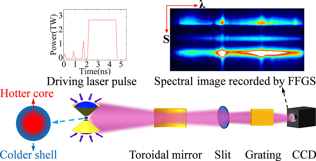
Figure 1 gives the schematic diagram of the flat-field grazing incident spectrometer, showing positions of the optics with respect to the two tip-to-tip cones. In the experiment, eight driving laser pulses at the wavelength of $0.351\;\mu \mathrm{m}$
carry total energy of
$0.351\;\mu \mathrm{m}$
carry total energy of $14\;\mathrm{kJ}$
in the duration of
$14\;\mathrm{kJ}$
in the duration of $4.7\;\mathrm{ns}$
to compress the spherical shell originally sealing each gold cone at its respective bases. The features of each optic element in the flat-field spectrometer are given in Appendix A. From Wien’s displacement law, the peak wavelength λ of the blackbody spectrum is given by
$4.7\;\mathrm{ns}$
to compress the spherical shell originally sealing each gold cone at its respective bases. The features of each optic element in the flat-field spectrometer are given in Appendix A. From Wien’s displacement law, the peak wavelength λ of the blackbody spectrum is given by $\lambda =b/T$
, where
$\lambda =b/T$
, where $b\simeq 250\;\mathrm{nm}\;{\mathrm{eV}}^{-1}$
is called Wien’s displacement constant and T is the temperature. For the temperature range of
$b\simeq 250\;\mathrm{nm}\;{\mathrm{eV}}^{-1}$
is called Wien’s displacement constant and T is the temperature. For the temperature range of $40\hbox{--} 200\;\mathrm{eV}$
, the corresponding wavelength range is
$40\hbox{--} 200\;\mathrm{eV}$
, the corresponding wavelength range is $1.25\hbox{--} 6.25\;\mathrm{nm}$
, which is the present measurement window. Outside this region, the radiation intensity gradient is small, and not distinguishable by a spectrometer for the given response efficiency.
$1.25\hbox{--} 6.25\;\mathrm{nm}$
, which is the present measurement window. Outside this region, the radiation intensity gradient is small, and not distinguishable by a spectrometer for the given response efficiency.
Schematic diagram of the flat-field grating spectrometer and the experimental setup. Also shown are the temporal profile of the eight laser pulses, the measured image of the soft X-ray spectra and a cartoon drawing of the hot dense plasma.

3 Main results
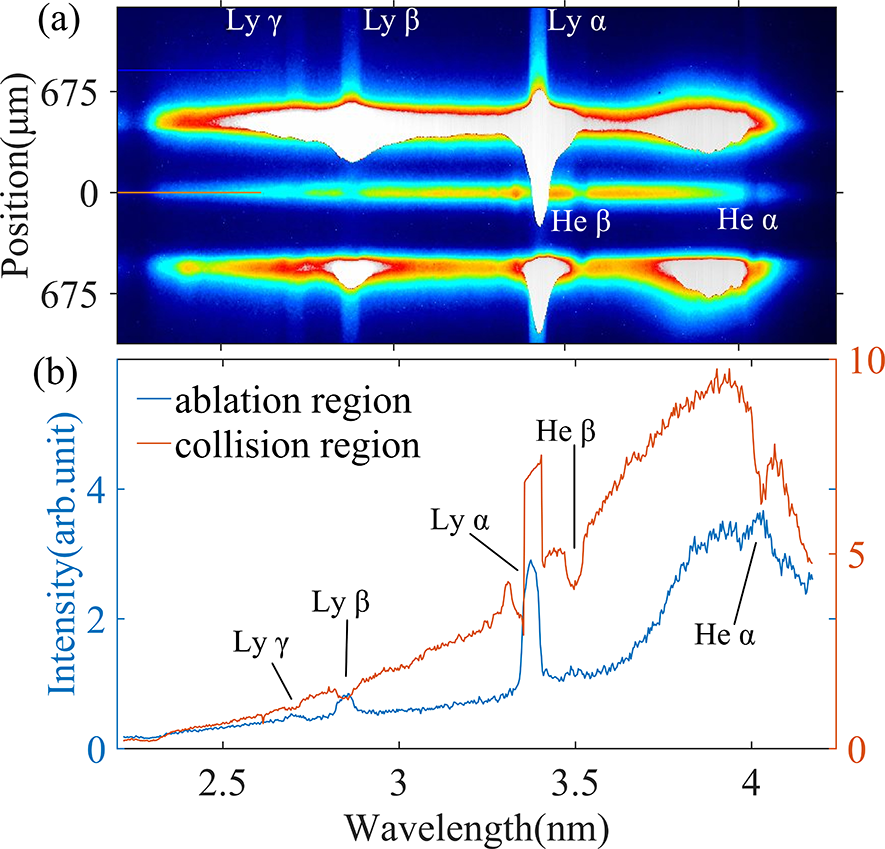
Figure 2 presents the measured spectra (Figure 2(a)) and the instrument efficiency-corrected spectra (Figure 2(b)) of carbon–deuterium (CD) plasma emissions. Figure 2(a) shows three characterized parts along the vertical direction. The top and the bottom parts are from the coronal plasma emissions generated by direct irradiation of the laser pulses on the CD shell. The distance between the lower edge of the top part and the upper edge of the bottom part corresponds to the separation between the open tips of two cones well aligned along their common axes. The separations are measured as 770 μm in Figure 2(a). From the corona of the laser-ablated plasma at the top and the bottom parts, three distinct emission lines are measured and identified as H-like carbon emissions. They are carbon’s Ly γ (2.69896 and 2.6990 nm), Ly β (2.84651 and 2.84663 nm) and Ly α (3.37341 and 3.37395 nm). The emission is weaker at the middle part of the spectral image in Figure 2(a). This emission part originates from the colliding compressed CD plasma ejected out with high velocity from the two cones’ open tip ends. By considering the sagittal magnification of the spectrometer and the size of the image area, the vertical length of the colliding plasma can be determined as $H=155\pm 6.75\;\mu \mathrm{m}$
. In Figure 2(a), the spectra at the middle present absorption lines of carbon’s He α (4.0268 nm), He β (3.4973 nm) and all the carbon’s H-like spectra. Figure 2(b) shows two efficiency-corrected spectra from the laser-ablated plasma region and the colliding plasma region in the experiment, respectively.
$H=155\pm 6.75\;\mu \mathrm{m}$
. In Figure 2(a), the spectra at the middle present absorption lines of carbon’s He α (4.0268 nm), He β (3.4973 nm) and all the carbon’s H-like spectra. Figure 2(b) shows two efficiency-corrected spectra from the laser-ablated plasma region and the colliding plasma region in the experiment, respectively.
Images of plasma emissions (a), as well as the wavelength calibrated carbon plasma spectra (b) after correction with the efficiencies of optics and a CCD. The blue solid line corresponds to the spectrum from the laser-ablated region. The orange solid line corresponds to the compressed and colliding plasma between two cone tips.

4 Data analysis
We employ four complementary methods to analyze the measured spectra, depending on different spectral features. For the coronal plasma, only emission lines from H-like carbon ions are observed, and the corresponding electron temperature and density are inferred from spectral line broadening. In the colliding region, the temperature and density of the outer shell are determined using both line-intensity ratios and line broadening, while the effective temperature of the hot core is obtained by fitting the continuum radiation with a Planckian function. Radiative hydrodynamics simulations and synthetic spectra are used to investigate the underlying physics in detail.
4.1 Analysis of the coronal region
The genetic algorithm (GA) provides a robust solution for navigating complex search regimes and mitigating the issue of local minima, and has been employed in the field of ICF experiments for the analysis of spectral data and other issues[ Reference Mukoyama20, Reference Wu, Yang, Ma, Zhang, Zhang, Yuan, Liu, Liu, Zhong, Zheng, Li and Zhang21].
The GA method helps in obtaining reliable plasma parameters from fitting the theoretical line profile ${I}_i^{\mathrm{theor}}$
of carbon’s Lyman series to the experimental line profile
${I}_i^{\mathrm{theor}}$
of carbon’s Lyman series to the experimental line profile ${I}_i^{\mathrm{exp}}$
. The individual fitness is defined as
${I}_i^{\mathrm{exp}}$
. The individual fitness is defined as ${\chi}^2=\sum \limits_{i=1}^N{\left({I}_i^{\mathrm{exp}}-{I}_i^{\mathrm{theor}}\right)}^2$
, where
${\chi}^2=\sum \limits_{i=1}^N{\left({I}_i^{\mathrm{exp}}-{I}_i^{\mathrm{theor}}\right)}^2$
, where $N$
is the number of experimental spectral data.
$N$
is the number of experimental spectral data.
To accurately compare the analytical results with the experimental data, we have already deconvoluted the experimental spectra to account for artificial factors such as the instrumental broadening of the synthetic profile. Among the three physical mechanisms contributing to spectral line broadening, that is, natural broadening, Doppler broadening and Stark broadening, the first two are calculated to be negligible. The Stark broadening ${\Gamma}_\mathrm{s}$
emerges as the primary cause of the spectral line broadening in plasmas[
Reference Man, Dong, Liu, Wei, Zhang, He and Wang22,
Reference Gigosos23] as the Coulomb collisions between electrons and emitting ions are of high occurrence. Here,
${\Gamma}_\mathrm{s}$
emerges as the primary cause of the spectral line broadening in plasmas[
Reference Man, Dong, Liu, Wei, Zhang, He and Wang22,
Reference Gigosos23] as the Coulomb collisions between electrons and emitting ions are of high occurrence. Here, ${\Gamma}_\mathrm{s}$
is calculated using the modified semi-empirical (MSE) formula[
Reference Dimitrijevic and Konjevic24,
Reference Dimitrijević25].
${\Gamma}_\mathrm{s}$
is calculated using the modified semi-empirical (MSE) formula[
Reference Dimitrijevic and Konjevic24,
Reference Dimitrijević25].
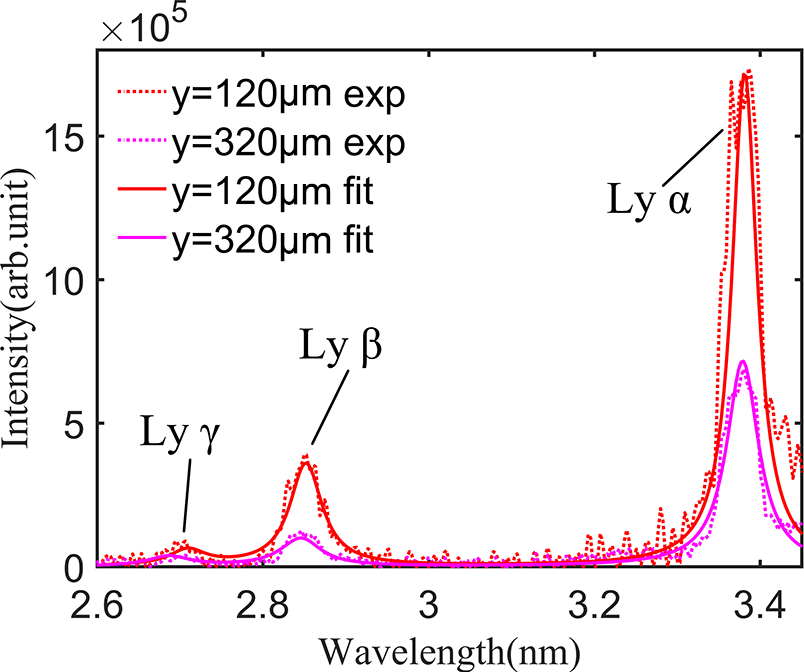
Figure 3 depicts the efficiency-corrected spectra at distances of $y=120\;\mathrm{and}\;320\;\mu \mathrm{m}$
, respectively, above the corona shell. The red and magenta solid lines are obtained through the GA’s fitting of the measured spectral profiles to the Lorentz type, with the width calculated by the MSE formula[
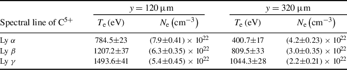
Reference Mossé, Génésio, Bonifaci and Calisti26]. The plasma properties obtained from C5+ Ly α, Ly β and Ly γ lines respectively are shown in Table 1. The maximum coronal temperature is given by
$y=120\;\mathrm{and}\;320\;\mu \mathrm{m}$
, respectively, above the corona shell. The red and magenta solid lines are obtained through the GA’s fitting of the measured spectral profiles to the Lorentz type, with the width calculated by the MSE formula[
Reference Mossé, Génésio, Bonifaci and Calisti26]. The plasma properties obtained from C5+ Ly α, Ly β and Ly γ lines respectively are shown in Table 1. The maximum coronal temperature is given by ${T}_{\mathrm{max}}\approx 1.1{I}_\mathrm{L}^{6/9}{\lambda}_\mathrm{L}^{4/9}{r}_\mathrm{f}^{4/9}\;(\mathrm{in\ keV})$
[
Reference Atzeni and Meyer-Ter-Vehn27], where
${T}_{\mathrm{max}}\approx 1.1{I}_\mathrm{L}^{6/9}{\lambda}_\mathrm{L}^{4/9}{r}_\mathrm{f}^{4/9}\;(\mathrm{in\ keV})$
[
Reference Atzeni and Meyer-Ter-Vehn27], where ${I}_\mathrm{L}$
represents the laser intensity in units of
${I}_\mathrm{L}$
represents the laser intensity in units of ${10}^{13}\;\mathrm{W}\;{\mathrm{cm}}^{-2}$
,
${10}^{13}\;\mathrm{W}\;{\mathrm{cm}}^{-2}$
, ${\lambda}_\mathrm{L}$
denotes the laser wavelength and
${\lambda}_\mathrm{L}$
denotes the laser wavelength and ${r}_\mathrm{f}$
corresponds to the focal spot size in millimeters. For the corresponding experimental laser parameters, it is approximately
${r}_\mathrm{f}$
corresponds to the focal spot size in millimeters. For the corresponding experimental laser parameters, it is approximately $1.68\;\mathrm{keV}$
. Since the measured signal is a time-integrated spectral signal, at a certain distance above the corona shell, the induced temperature and electron density ranges are relatively broad, although both fall within acceptable limits. The effective temperatures (density) determined from carbon’s Ly β and Ly γ are slightly higher (lower) than that from carbon’s Ly α, because plasmas of higher effective temperature have more C5+ ions with electron configurations of 1d and 1f. Since hot plasmas expand much faster, carbon’s Ly β and Ly γ emissions are mostly from the plasma edge. The electron effective temperature range is quite broad as the spectra are time-integrated. The electron density continues to decrease as the measured plasma moves far from the cone.
$1.68\;\mathrm{keV}$
. Since the measured signal is a time-integrated spectral signal, at a certain distance above the corona shell, the induced temperature and electron density ranges are relatively broad, although both fall within acceptable limits. The effective temperatures (density) determined from carbon’s Ly β and Ly γ are slightly higher (lower) than that from carbon’s Ly α, because plasmas of higher effective temperature have more C5+ ions with electron configurations of 1d and 1f. Since hot plasmas expand much faster, carbon’s Ly β and Ly γ emissions are mostly from the plasma edge. The electron effective temperature range is quite broad as the spectra are time-integrated. The electron density continues to decrease as the measured plasma moves far from the cone.
The measured spectra and the genetic algorithm fitting curves at 120 and 320 μm above the corona region.

Parameters of the ablated plasma at different distances from the corona.

4.2 Analysis of the colliding region
Figure 2(b) shows a comparison between spectra of the compressed plasma and the laser-direct-ablated plasma. It is reasonable to figure that the continuum comes from a hotter inner plasma region where electron density is larger than ${10}^{24}\;{\mathrm{cm}}^{-3}$
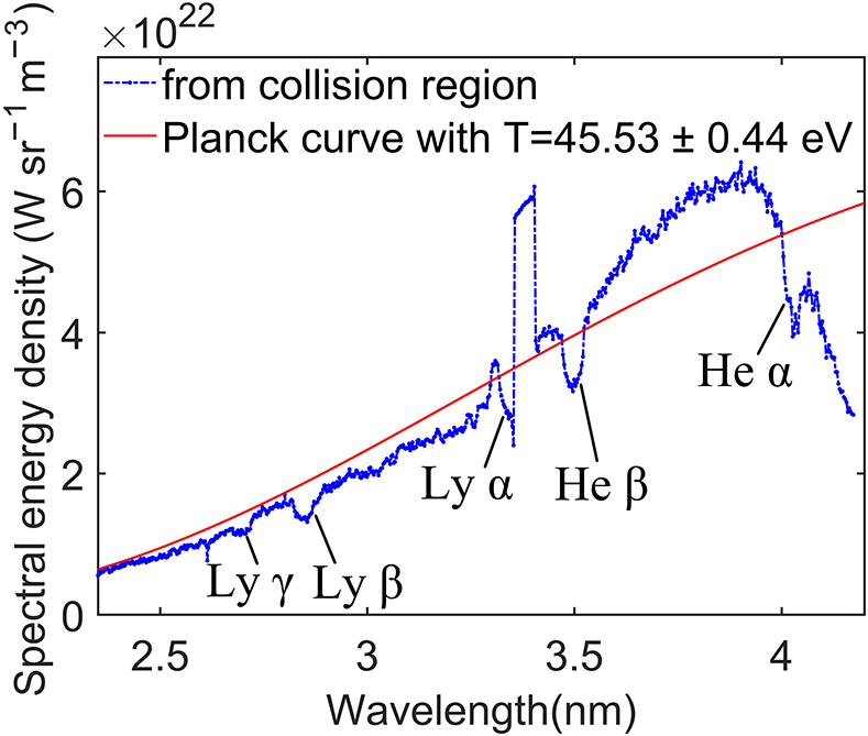
since the spectral lines disappear. The continuum propagates outward through a colder outer plasma region where ground-state C5+ ions still exist and absorb the continuum at corresponding frequencies. As will be shown in the theoretical model below, photons in the optically thick colliding plasma undergo multiple absorption and re-emission processes, and thermalize into a blackbody spectrum, which can be characterized by Planck’s law. At an absolute effective temperature
${10}^{24}\;{\mathrm{cm}}^{-3}$
since the spectral lines disappear. The continuum propagates outward through a colder outer plasma region where ground-state C5+ ions still exist and absorb the continuum at corresponding frequencies. As will be shown in the theoretical model below, photons in the optically thick colliding plasma undergo multiple absorption and re-emission processes, and thermalize into a blackbody spectrum, which can be characterized by Planck’s law. At an absolute effective temperature ${T}_{\mathrm{eff}}$
, the spectral radiation of an object at wavelength
${T}_{\mathrm{eff}}$
, the spectral radiation of an object at wavelength $\lambda$
is given by the following:
$\lambda$
is given by the following:
 $$\begin{align}{B}_\mathrm{It}=\frac{2{hc}^2}{\lambda^5}\frac{1}{\exp \left( hc/\lambda {kT}_{\mathrm{eff}}-1\right)},\end{align}$$
where $k$
is the Boltzmann constant,
$k$
is the Boltzmann constant, $h$
is the Planck constant,
$h$
is the Planck constant, $c$
is the speed of light in vacuum and the unit of
$c$
is the speed of light in vacuum and the unit of ${B}_{\mathrm{It}}$
is
${B}_{\mathrm{It}}$
is $\mathrm{W}\cdot {\mathrm{sr}}^{\hbox{--} 1}\cdot {\mathrm{m}}^{\hbox{--} 3}$
.
$\mathrm{W}\cdot {\mathrm{sr}}^{\hbox{--} 1}\cdot {\mathrm{m}}^{\hbox{--} 3}$
.
In the measured experimental spectrum, the absolute number of photons ${N}_{\mathrm{total}}$
within the wavelength range between 2.2 and 4.2 nm can be obtained. By taking into account the observed solid angle
${N}_{\mathrm{total}}$
within the wavelength range between 2.2 and 4.2 nm can be obtained. By taking into account the observed solid angle ${\varOmega}_{\mathrm{FFS}}=5.625\times {10}^{\hbox{--} 5}\;\mathrm{sr}$
covered by the flat-field spectrometer, the duration of the self-emission plasmas
${\varOmega}_{\mathrm{FFS}}=5.625\times {10}^{\hbox{--} 5}\;\mathrm{sr}$
covered by the flat-field spectrometer, the duration of the self-emission plasmas ${t}_\mathrm{d}=500\;\mathrm{ps}$
for the collision process, the surface area
${t}_\mathrm{d}=500\;\mathrm{ps}$
for the collision process, the surface area ${S}_{\mathrm{thermal}}=8.4496\times {10}^{-8}\;{\mathrm{m}}^2$
of the observed hotter core and the wavelength increment
${S}_{\mathrm{thermal}}=8.4496\times {10}^{-8}\;{\mathrm{m}}^2$
of the observed hotter core and the wavelength increment $\Delta \lambda$
, the radiation can be calculated:
$\Delta \lambda$
, the radiation can be calculated:
 $$\begin{align}{B}_\mathrm{Ie}=({N}_{\mathrm{total}}\cdot hc)/({\varOmega}_{\mathrm{FFS}} \cdot {t}_\mathrm{d} \cdot {S}_{\mathrm{thermal}} \cdot \lambda \cdot \varDelta \lambda) .\end{align}$$
Figure 4 depicts the fitting results of the theoretical Planck radiation distribution ${B}_{\mathrm{It}}$
and the experimental data
${B}_{\mathrm{It}}$
and the experimental data ${B}_\mathrm{Ie}$
of the compressed plasmas between the two cone tips. The blue dot-dot-dashed line represents the efficiency-corrected spectral radiation. The red solid line corresponds to the blackbody radiation spectra at the given electron effective temperature, that is,
${B}_\mathrm{Ie}$
of the compressed plasmas between the two cone tips. The blue dot-dot-dashed line represents the efficiency-corrected spectral radiation. The red solid line corresponds to the blackbody radiation spectra at the given electron effective temperature, that is, $45.53\pm 0.44\;\mathrm{eV}$
.
$45.53\pm 0.44\;\mathrm{eV}$
.
Fitting of the continuous spectra with the blackbody radiation formula.

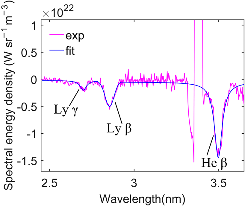
In Figure 5, the magenta line presents the absorption features after subtraction of the fitted blackbody radiation curve of the measured spectra from the dense plasma emission. The blue line represents the optimal fit achieved using the GA. Combined with the MSE formula[
Reference Dimitrijevic and Konjevic24,
Reference Dimitrijević25], the electron effective temperature is determined to be $32.35\pm 4.15\;\mathrm{eV}$
, and the electron density is
$32.35\pm 4.15\;\mathrm{eV}$
, and the electron density is $(1.45\pm 0.35)\times {10}^{23}\;{\mathrm{cm}}^{\hbox{--} 3}$
.
$(1.45\pm 0.35)\times {10}^{23}\;{\mathrm{cm}}^{\hbox{--} 3}$
.
The GA fitted to the absorption spectral lines.

By using the relationship between the spectral integration intensity and the ground-state particle number density, the number densities of the electron configuration of 1s (C5+) and 1s2 (C4+) ground states can be obtained. Taking into consideration Ly-β1 and He-β as an example, the intensity ratio computed using the Saha equation is as follows:
 $$\begin{align}\frac{I_{\mathrm{saha},\mathrm{Ly}\hbox{-} \beta 1}}{I_{\mathrm{saha},\mathrm{He}\hbox{-} \beta}}&=\frac{f_\mathrm{abs}\cdot {N}_{1\mathrm{s}}\cdot {{g}}_{1\mathrm{s}}}{{f^{\hbox{'}}}_\mathrm{abs}\cdot {N}_{1{\mathrm{s}}^2}\cdot {{g}}_{1{\mathrm{s}}^2}}\nonumber\\&=\left(\frac{\frac{{{g}}_{1\mathrm{s}}}{{{g}}_{3\mathrm{p}}}\cdot \frac{{{m}}_\mathrm{e}c{\varepsilon}_0}{2\pi {e}^2}\cdot {A}_{\mathrm{Ly}\hbox{-} \beta 1}}{\frac{{{g}}_{1{\mathrm{s}}^2}}{{{g}}_{3{\mathrm{p}}^2}}\cdot \frac{{\mathrm{m}}_\mathrm{e}c{\varepsilon}_0}{2\pi {e}^2}\cdot {A}_{\mathrm{He}\hbox{-} \beta}}\right)\cdot \frac{{{g}}_{1\mathrm{s}}\cdot {\lambda^2}_{\mathrm{Ly}\hbox{-} \beta 1}\cdot {N}_{1\mathrm{s}}}{{{g}}_{1{\mathrm{s}}^2}\cdot {\lambda^2}_{\mathrm{He}\hbox{-} \beta}\cdot {N}_{1{\mathrm{s}}^2}},\end{align}$$
where ${{g}}_{1\mathrm{s}}$
and
${{g}}_{1\mathrm{s}}$
and ${{g}}_{1\mathrm{s}^2}$
represent the statistical weights of the ground state for Lyman-β1 and He-β, while
${{g}}_{1\mathrm{s}^2}$
represent the statistical weights of the ground state for Lyman-β1 and He-β, while ${{g}}_{3\mathrm{p}}$
and
${{g}}_{3\mathrm{p}}$
and ${{g}}_{3\mathrm{p}^2}$
are the corresponding excited states. Here,
${{g}}_{3\mathrm{p}^2}$
are the corresponding excited states. Here, ${A}_{\mathrm{Ly}\hbox{-} \beta 1}$
and
${A}_{\mathrm{Ly}\hbox{-} \beta 1}$
and ${A}_{\mathrm{He}\hbox{-} \beta}$
are the spontaneous transition probabilities for
${A}_{\mathrm{He}\hbox{-} \beta}$
are the spontaneous transition probabilities for ${\lambda}_{\mathrm{Ly}\hbox{-} \beta 1}=2.84651\;\mathrm{nm}$
and
${\lambda}_{\mathrm{Ly}\hbox{-} \beta 1}=2.84651\;\mathrm{nm}$
and ${\lambda}_{\mathrm{He}\hbox{-} \beta}=3.4973\;\mathrm{nm}$
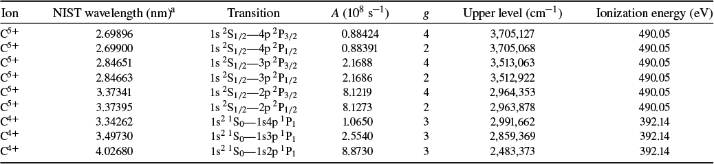
, respectively. These statistical weights and transition probabilities are listed in Table 1. Further
${\lambda}_{\mathrm{He}\hbox{-} \beta}=3.4973\;\mathrm{nm}$
, respectively. These statistical weights and transition probabilities are listed in Table 1. Further ${f}_{\mathrm{abs}}$
and
${f}_{\mathrm{abs}}$
and ${f^{\hbox{'}}}_{\mathrm{abs}}$
denote the absorption oscillator strengths for Ly-β1 and He-β, respectively,
${f^{\hbox{'}}}_{\mathrm{abs}}$
denote the absorption oscillator strengths for Ly-β1 and He-β, respectively, ${N}_{1\mathrm{s}}$
and
${N}_{1\mathrm{s}}$
and ${N}_{1{\mathrm{s}}^2}$
are the number densities of the ground state,
${N}_{1{\mathrm{s}}^2}$
are the number densities of the ground state, ${{m}}_\mathrm{e}$
is the electron mass,
${{m}}_\mathrm{e}$
is the electron mass, ${\varepsilon}_0$
is the vacuum permittivity and
${\varepsilon}_0$
is the vacuum permittivity and $e$
is the elementary charge. The used atomic data are given in Appendix B.
$e$
is the elementary charge. The used atomic data are given in Appendix B.
The number ratio of C5+ and C4+ is determined to be ${N}_{1\mathrm{s}}$
:
${N}_{1\mathrm{s}}$
: ${N}_{1\mathrm{s}^2}\sim 0.180$
based on the ratio of integrated intensities of carbon’s Ly-β1 to that of carbon’s He-β. The ionization state distribution is also calculated using the ratio of integrated intensities of carbon’s Ly-γ1 to carbon’s He-β, resulting in
${N}_{1\mathrm{s}^2}\sim 0.180$
based on the ratio of integrated intensities of carbon’s Ly-β1 to that of carbon’s He-β. The ionization state distribution is also calculated using the ratio of integrated intensities of carbon’s Ly-γ1 to carbon’s He-β, resulting in ${N}_{1\mathrm{s}}$
:
${N}_{1\mathrm{s}}$
: ${N}_{1\mathrm{s}^2}\sim 0.178$
, which is consistent with the former calculation. Combining the Saha–Boltzmann equation and the GA for adjacent ionization states, the electron effective temperature of the colder carbon shell is determined to be
${N}_{1\mathrm{s}^2}\sim 0.178$
, which is consistent with the former calculation. Combining the Saha–Boltzmann equation and the GA for adjacent ionization states, the electron effective temperature of the colder carbon shell is determined to be $34.26\pm 2.12\;\mathrm{eV}$
, and the electron density is
$34.26\pm 2.12\;\mathrm{eV}$
, and the electron density is $(1.03\pm 0.21)\times {10}^{23}\;{\mathrm{cm}}^{-3}$
, which are close to the plasma parameters obtained by combining the GA and MSE methods.
$(1.03\pm 0.21)\times {10}^{23}\;{\mathrm{cm}}^{-3}$
, which are close to the plasma parameters obtained by combining the GA and MSE methods.
4.3 Simulations
To get a better understanding of the physics underlying the experimental phenomena, we carried out radiation hydrodynamics simulations with the open-source code FLASH[ Reference Fryxell, Olson, Ricker, Timmes, Zingale, Lamb, Macneice, Rosner, Truran and Tufo28– Reference Tzeferacos, Fatenejad, Flocke, Graziani, Gregori, Lamb, Lee, Meinecke, Scopatz and Weide30]. The Eulerian hydrodynamic equations of the three-temperature model in two-dimensional (2D) cylindrical geometry are solved with the radiation transport approximated by the multi-group diffusion model. The tabulated equations of state (EOSs) and opacities are generated by PROPACEOS code. The ray tracing method of three dimensions in two dimensions (3D-in-2D) is employed to calculate the laser energy deposition.
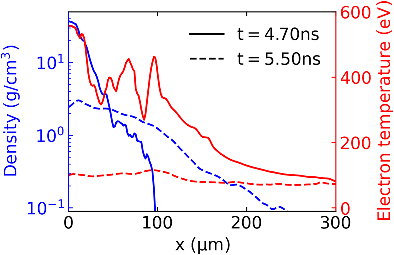
The density and temperature slices of the simulation are given in Appendix C. The simulation assumes optimized conditions, utilizing the theoretically optimized laser pulse shape depicted in Figure 1. Nanosecond laser pulses ablate the target, ionizing part of the shell target in the laser-focal spot and generating a corona plasma layer above the shell. The rest of the target shells are accelerated to an average velocity of several hundred kilometers per second within the gold cone configuration. At the moment of collision, the stagnated and shocked plasma (∼ $100\;\mu \mathrm{m}$
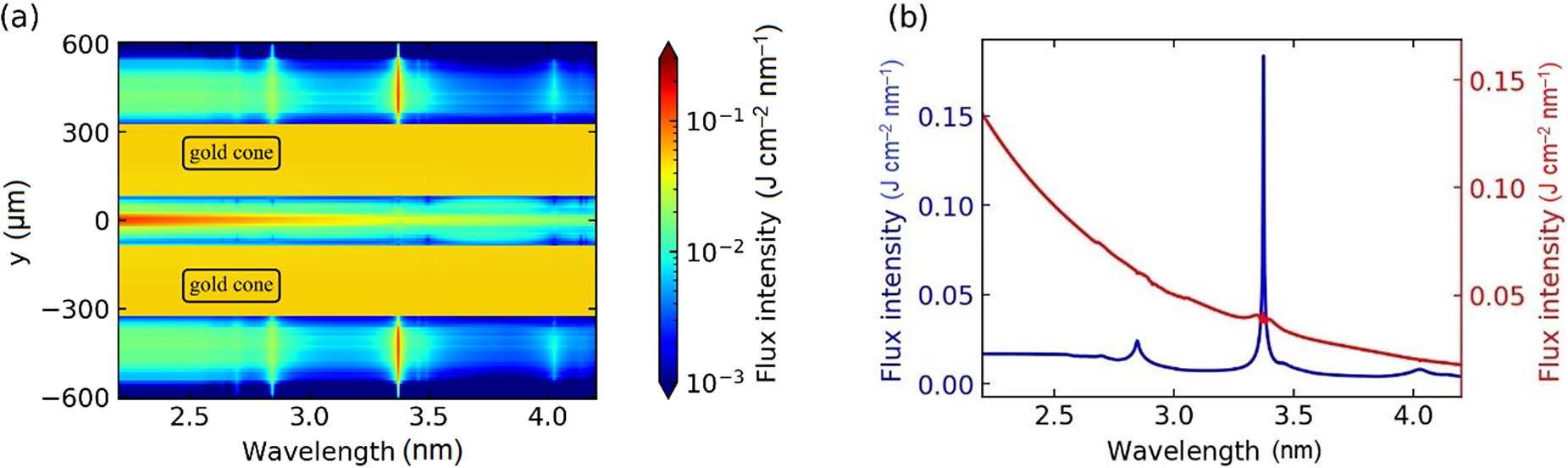
) exhibits a sharp density gradient in the equatorial plane, and a gradual temperature decline along the radial direction, as shown by the solid line in Figure 6. The plasma density under these conditions is sufficiently high, rendering the shocked plasma highly opaque to soft X-rays, consistent with experimental measurements. This means photons originally from the deep inner part of the plasma experience multiple cycles of absorption and re-emission before escaping, thermalizing the spectra into a Planck one. This behavior starkly contrasts with the corona plasma, where optically thin conditions restrict energy exchange processes, and allow discrete emission lines to dominate the spectra, as shown in Figures 7 and 2.
$100\;\mu \mathrm{m}$
) exhibits a sharp density gradient in the equatorial plane, and a gradual temperature decline along the radial direction, as shown by the solid line in Figure 6. The plasma density under these conditions is sufficiently high, rendering the shocked plasma highly opaque to soft X-rays, consistent with experimental measurements. This means photons originally from the deep inner part of the plasma experience multiple cycles of absorption and re-emission before escaping, thermalizing the spectra into a Planck one. This behavior starkly contrasts with the corona plasma, where optically thin conditions restrict energy exchange processes, and allow discrete emission lines to dominate the spectra, as shown in Figures 7 and 2.
The collision plasma’s ( $y=0\;\mu \mathrm{m}$
) radial density (blue line) and electron temperature (red line) at collision time
$y=0\;\mu \mathrm{m}$
) radial density (blue line) and electron temperature (red line) at collision time $t=4.7\;\mathrm{ns}$
(solid line) and late time
$t=4.7\;\mathrm{ns}$
(solid line) and late time $t=5.5\;\mathrm{ns}$
(dashed line).
$t=5.5\;\mathrm{ns}$
(dashed line).

The spectral calculations matching experimental measurements were performed using the collisional-radiative code Spect3D[
Reference Macfarlane, Golovkin, Wang, Woodruff and Pereyra31]. Under the local thermal equilibrium (LTE) assumption, we computed the electron population and derived free–free, free–bound, bound–bound opacities. The one-dimensional (1D) radiative transfer equation was then solved along each line of sight (LOS). To replicate experimental conditions, the intensity was integrated horizontally. Figure 7 displays the synthetic time-integrated flux intensity as a function of vertical position and wavelength. Gold cones are represented as masks to illustrate their strong attenuation effects. The results reveal prominent absorption and emission lines superimposed on a continuum blackbody spectrum, closely resembling experimental observations. Notably, the primary flux contribution in the collision region occurs precisely at the collision time. The calculated blackbody temperature at the collision region’s edge (where density falls below 0.1 g cm–3) approximates 182 eV, with minor variations depending on grid resolution and spatial position. As illustrated in Figure 6, this temperature corresponds to the optical depth $\tau =1$
, which is also used in our analytical model. To directly compare the results of the simulations with experiments, critical caveats must be noted. First, the calculation omitted the opacity of water components still existing in the chamber, which obscures the radiation around 1 and 6 nm. Second, detector response effects are not included in the calculation. Third, there is gold plasma contamination at the plasma edge. Previous simulations[
Reference Zhang, Wu, Yang, Ma, Cui, Jiang and Zhang32] indicate that gold migrates to the colliding plasma’s edge, forming a high-opacity layer that attenuates X-ray transmission – a phenomenon corroborated by Cu-Kα diagnostics[
Reference Zhang, Yuan, Zhang, Liu, Fang, Zhang, Liu, Zhao, Dong, Liu, Dai, Gu, Li, Zheng, Zhong and Zhang12]. This contamination likely alters radiative transport pathways and suppresses the measured temperatures.
$\tau =1$
, which is also used in our analytical model. To directly compare the results of the simulations with experiments, critical caveats must be noted. First, the calculation omitted the opacity of water components still existing in the chamber, which obscures the radiation around 1 and 6 nm. Second, detector response effects are not included in the calculation. Third, there is gold plasma contamination at the plasma edge. Previous simulations[
Reference Zhang, Wu, Yang, Ma, Cui, Jiang and Zhang32] indicate that gold migrates to the colliding plasma’s edge, forming a high-opacity layer that attenuates X-ray transmission – a phenomenon corroborated by Cu-Kα diagnostics[
Reference Zhang, Yuan, Zhang, Liu, Fang, Zhang, Liu, Zhao, Dong, Liu, Dai, Gu, Li, Zheng, Zhong and Zhang12]. This contamination likely alters radiative transport pathways and suppresses the measured temperatures.
(a) Calculated time-integrated, spatially resolved spectrum and (b) time-integrated intensity of corona plasma (blue line, $y=400\;\mu \mathrm{m}$
) and collision plasma (red line,
$y=400\;\mu \mathrm{m}$
) and collision plasma (red line, $y=0\;\mu \mathrm{m}$
).
$y=0\;\mu \mathrm{m}$
).

4.4 Analytical model
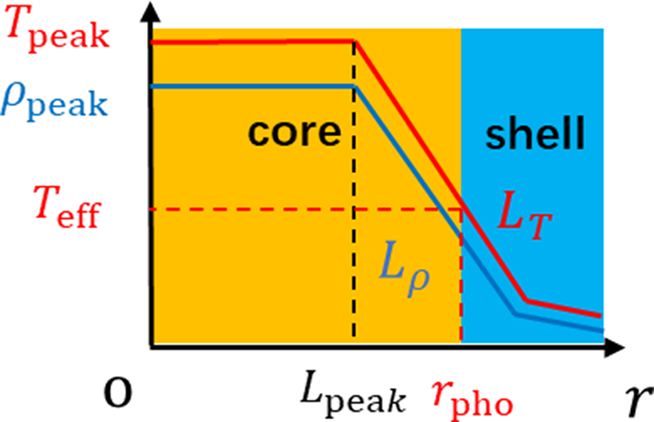
To estimate the edge scale length of the colliding plasma and show the rationality of the Planck law’s application in plasma determination, we give a simple analytic model, which assumes that the density and temperature decay exponentially in scale lengths ${L}_{\rho }$
and
${L}_{\rho }$
and ${L}_T$
, respectively, as shown in Figure 8. The scale length is defined as
${L}_T$
, respectively, as shown in Figure 8. The scale length is defined as ${L}_a\equiv a/\left|\frac{\mathrm{d}a}{\mathrm{d}r}\right|=1/\left|\frac{\mathrm{d}\ln a}{\mathrm{d}r}\right|$
, where
${L}_a\equiv a/\left|\frac{\mathrm{d}a}{\mathrm{d}r}\right|=1/\left|\frac{\mathrm{d}\ln a}{\mathrm{d}r}\right|$
, where $a$
denotes density
$a$
denotes density $\rho$
or temperature
$\rho$
or temperature $T$
. The optical depth is given by the following:
$T$
. The optical depth is given by the following:
 $$\begin{align}\mathrm{d}\tau =\rho \kappa \mathrm{d}r,\end{align}$$
The radial density and temperature profiles for the colliding plasma. The y-axis is on a logarithmic scale.

where $\kappa$
is the opacity, which is dominated by the free–free opacity, related to the inverse-bremsstrahlung absorption process for the plasma parameters of the colliding plasma. We stay agnostic about the opacity components and assume they are a function of density and temperature, for example,
$\kappa$
is the opacity, which is dominated by the free–free opacity, related to the inverse-bremsstrahlung absorption process for the plasma parameters of the colliding plasma. We stay agnostic about the opacity components and assume they are a function of density and temperature, for example, $\kappa ={{C}}_{\kappa}{\rho}^{\alpha}{{T}}^{\beta}$
, where
$\kappa ={{C}}_{\kappa}{\rho}^{\alpha}{{T}}^{\beta}$
, where ${{C}}_{\kappa}$
is a constant that depends only on the components of the plasma, for instance, the averaged atomic numbers
${{C}}_{\kappa}$
is a constant that depends only on the components of the plasma, for instance, the averaged atomic numbers $\overline{A},\ \mathrm{and} \ \alpha\;\mathrm{and}\;\beta$
are real numbers. By substituting
$\overline{A},\ \mathrm{and} \ \alpha\;\mathrm{and}\;\beta$
are real numbers. By substituting $\kappa$
, we get the following:
$\kappa$
, we get the following:
 $$\begin{align}\mathrm{d}\tau &={C}_{\kappa }{\rho}^{\alpha +1}{T}^{\beta}\mathrm{d}r\nonumber\\&={C}_{\kappa, \mathrm{peak}}\exp \left(-\left(\frac{\alpha +1}{L_{\rho }}+\frac{\beta }{L_T}\right)\left(r-{L}_{\mathrm{peak}}\right)\right)\mathrm{d}r,\end{align}$$
where ${C}_{\kappa, \mathrm{peak}}={C}_{\kappa }{\rho}_{\mathrm{peak}}^{\alpha +1}{T}_{\mathrm{peak}}^{\beta }=1/{\lambda}_{\mathrm{peak}}$
is the absorption coefficient and
${C}_{\kappa, \mathrm{peak}}={C}_{\kappa }{\rho}_{\mathrm{peak}}^{\alpha +1}{T}_{\mathrm{peak}}^{\beta }=1/{\lambda}_{\mathrm{peak}}$
is the absorption coefficient and ${\lambda}_{\mathrm{peak}}$
is the mean free path of the photon of colliding plasma in the peak region. Integrate the above equation, with the assumption that
${\lambda}_{\mathrm{peak}}$
is the mean free path of the photon of colliding plasma in the peak region. Integrate the above equation, with the assumption that $\left(\frac{\alpha +1}{L_\rho}+\frac{\beta }{L_T}\right)>0$
. Otherwise, the edge is unphysically more opaque than the peak region and tends to diverse toward infinity, and therefore truncations of radial profiles are needed. Then, the optical depth of the edge region is as follows:
$\left(\frac{\alpha +1}{L_\rho}+\frac{\beta }{L_T}\right)>0$
. Otherwise, the edge is unphysically more opaque than the peak region and tends to diverse toward infinity, and therefore truncations of radial profiles are needed. Then, the optical depth of the edge region is as follows:
 $$\begin{align}{\tau}_{\mathrm{edge}}(r)&=\underset{r-{L}_{\mathrm{peak}}}{\overset{\infty }{\int }}\mathrm{d}\tau\nonumber\\& ={C}_{\kappa, \mathrm{peak}}\frac{\exp \left(-\left(\frac{\alpha +1}{L_{\rho }}+\frac{\beta }{L_T}\right)\left(r-{L}_{\mathrm{peak}}\right)\right)}{\frac{\alpha +1}{L_{\rho }}+\frac{\beta }{L_T}}.\end{align}$$
The total optical depth of plasma at the center is as follows:
 $$\begin{align}{\tau}_{\mathrm{peak}}&={C}_{\kappa, \mathrm{peak}}{L}_{\mathrm{peak}}+{\tau}_{\mathrm{edge}}\left({L}_{\mathrm{peak}}\right)\nonumber\\ &={C}_{\kappa, \mathrm{peak}}\left({L}_{\mathrm{peak}}+1/\left(\frac{\alpha +1}{L_{\rho }}+\frac{\beta }{L_T}\right)\right).\end{align}$$
The inner region $\left(r<{L}_{\mathrm{peak}}\right)$
is a plateau with constant peak density
$\left(r<{L}_{\mathrm{peak}}\right)$
is a plateau with constant peak density ${\rho}_{\mathrm{peak}}$
and temperature
${\rho}_{\mathrm{peak}}$
and temperature ${T}_{\mathrm{peak}}$
. In the edge region
${T}_{\mathrm{peak}}$
. In the edge region $\left({L}_{\mathrm{peak}}<r<{L}_{\mathrm{peak}}+{L}_{\rho/T}\right)$
, density and temperature exponentially decay in scale lengths
$\left({L}_{\mathrm{peak}}<r<{L}_{\mathrm{peak}}+{L}_{\rho/T}\right)$
, density and temperature exponentially decay in scale lengths ${L}_{\rho }$
and
${L}_{\rho }$
and ${L}_T$
, respectively. The effective temperature of the colliding plasma in the edge region is indicated with red dashed lines.
${L}_T$
, respectively. The effective temperature of the colliding plasma in the edge region is indicated with red dashed lines.
The Planckian-like continuum spectrum can only be obtained when the colliding plasma is optically thick. That gives a constraint on the validity of Planck’s law application in temperature estimation. In our model, this happens when ${\lambda}_{\mathrm{peak}}\ll {L}_{\mathrm{peak}}$
. Similar to a stellar (e.g., white dwarf) photosphere, the effective temperature of the colliding plasma is the temperature where the optical depth equals unity
${\lambda}_{\mathrm{peak}}\ll {L}_{\mathrm{peak}}$
. Similar to a stellar (e.g., white dwarf) photosphere, the effective temperature of the colliding plasma is the temperature where the optical depth equals unity $\left(\tau \left({r}_{\mathrm{pho}}\right)=1\right)$
or
$\left(\tau \left({r}_{\mathrm{pho}}\right)=1\right)$
or ${T}_{\mathrm{eff}}=T\left({r}_{\mathrm{pho}}\right)$
. Then we finally arrive at the following:
${T}_{\mathrm{eff}}=T\left({r}_{\mathrm{pho}}\right)$
. Then we finally arrive at the following:
 $$\begin{align}{T}_{\mathrm{eff}}={T}_{\mathrm{peak}}{\left(\left(\frac{\alpha +1}{L_{\rho }}+\frac{\beta }{L_T}\right){\lambda}_{\mathrm{peak}}\right)}^{\frac{1}{\left(\alpha +1\right){L}_T/{L}_{\rho }+\beta }}.\end{align}$$
The formula indicates that the effective temperature of colliding plasma is related to the temperature of the peak region and is sensitive to the scale length of the edge region and the opacity components. As an illustration, we consider a simple case where the opacity is dominated by free–free opacity for the given frequency of photons, $\alpha =1,\beta =-0.5$
, the scale length of density and temperature is the same,
$\alpha =1,\beta =-0.5$
, the scale length of density and temperature is the same, ${L}_{\rho }={L}_T\sim 20\;\mu \mathrm{m}$
, the mean free path of the photon in the peak region is
${L}_{\rho }={L}_T\sim 20\;\mu \mathrm{m}$
, the mean free path of the photon in the peak region is ${\lambda}_{\mathrm{peak}}\sim {10}^{-4}\;\mathrm{cm}$
and the ratio of the effective temperature over peak temperature is
${\lambda}_{\mathrm{peak}}\sim {10}^{-4}\;\mathrm{cm}$
and the ratio of the effective temperature over peak temperature is ${T}_{\mathrm{eff}}/{T}_{\mathrm{peak}}\sim 1/6$
. Considering the case with a peak temperature of
${T}_{\mathrm{eff}}/{T}_{\mathrm{peak}}\sim 1/6$
. Considering the case with a peak temperature of $300\;\mathrm{eV}$
[
Reference Fang, Zhang, Dong, Zhang, Zhang, Yuan, Li and Zhang11], the effective temperature from our estimate is roughly
$300\;\mathrm{eV}$
[
Reference Fang, Zhang, Dong, Zhang, Zhang, Yuan, Li and Zhang11], the effective temperature from our estimate is roughly $50\;\mathrm{eV}$
by using the chosen values of the length scale and model of opacity. This yields a peak-to-effective temperature ratio of 6, which is close to the measured value.
$50\;\mathrm{eV}$
by using the chosen values of the length scale and model of opacity. This yields a peak-to-effective temperature ratio of 6, which is close to the measured value.
In general, the ionization degree for the plasma varies drastically in the edge region, and the leading component of opacity may change from free–free opacity to opacity related to atomic bound states due to recombination with plasma cooling. Thus, a more reliable calculation of effective temperature needs more accurate modeling of opacity.
4.5 Discussion
To interpret the measured effective temperature, in Section 4.4, we assume the isolated colliding plasma to have a core of flat distributions of density and temperature with exponentially decaying edges. This model is supported by two main physical considerations. The first is that the shock dynamics tend to flatten strong density gradients. The second is that in degenerate plasma interiors, efficient thermal conduction acts to reduce strong temperature gradients. The density and temperature profiles derived from axis-symmetric inversion further support this structure[ Reference Fang, Zhang, Dong, Zhang, Zhang, Yuan, Li and Zhang11, Reference Zhang, Yuan, Zhang, Liu, Fang, Zhang, Liu, Zhao, Dong, Liu, Dai, Gu, Li, Zheng, Zhong and Zhang12]. In addition, the collision of jets forms a plasma–vacuum interface where the edge is determined by rarefaction wave propagation, while simulations confirm that shock fronts propagating outward from the collision region define the plasma boundary. However, the realistic spatial distribution depends on multiple factors including collision symmetry, entropy transport through conduction and radiation processes and the expansion dynamics of the plasma itself. This highlights the need for future work involving detailed spatially and temporally resolved diagnostics to properly characterize the degenerate plasma in a very small volume and a very short time interval.
In dense plasmas, the atomic ionization potentials are reduced compared to the case of a single atom, an effect known as the ionization potential depression (IPD)[ Reference Kritcher, Swift, Döppner, Bachmann, Benedict, Collins, DuBois, Elsner, Fontaine, Gaffney and Hamel8, Reference Kraus, Chapman, Kritcher, Baggott, Bachmann, Collins, Glenzer, Hawreliak, Kalantar, Landen and Ma33, Reference Hoarty, Allan, James, Brown, Hobbs, Hill, Harris, Morton, Brookes, Shepherd and Dunn34]. Another factor that affects atomic ionization is Pauli blocking, when free electrons fill all available states below the Fermi energy. Both effects can induce shifts in spectral line series and bound-free transitions. These effects appear negligible in our current measurements. The measured radiation primarily originates from the lower-density edge region, but the forementioned quantum effects should become significant for the degenerate inner region and unshocked jets[ Reference Young16]. The absorption features in our spectra occur mostly for the low-energy photons, suggesting that extending our measurements to higher energy bands could reveal radiation from the inner plasma regions. Furthermore, adapting our diagnostic approach to include time resolution while maintaining focus on the colliding plasma would improve the signal-to-noise ratios and enable more detailed investigation of the collision’s spatiotemporal evolution. Of course, all of these prospects require the realization of a bright and large degenerate plasma as the signal emission source.
5 Summary
The DCI scheme provides a promising approach to produce and study well-isolated dense plasma systems in quantum degeneracy. The soft X-ray spectrometry showed that the experimentally achieved plasma at present has a structure consisting of a hotter core and a colder shell. The core is in a state of high effective temperature of $45.53\pm 0.44\;\mathrm{eV}$
. The outer colder shell has a density around
$45.53\pm 0.44\;\mathrm{eV}$
. The outer colder shell has a density around ${10}^{23}\;{\mathrm{cm}}^{\hbox{--} 3}$
and an effective temperature of
${10}^{23}\;{\mathrm{cm}}^{\hbox{--} 3}$
and an effective temperature of $34.26\pm 2.12\;\mathrm{eV}$
. The FLASH simulations predict a higher temperature, indicating the existence of the non-ideal effects in the realistic measurements. It is believed that researches based on the DCI’s hot dense plasmas can make significant potential contributions to studies of the properties of matters inside giant planets and brown and white dwarfs[
Reference Fortov35].
$34.26\pm 2.12\;\mathrm{eV}$
. The FLASH simulations predict a higher temperature, indicating the existence of the non-ideal effects in the realistic measurements. It is believed that researches based on the DCI’s hot dense plasmas can make significant potential contributions to studies of the properties of matters inside giant planets and brown and white dwarfs[
Reference Fortov35].
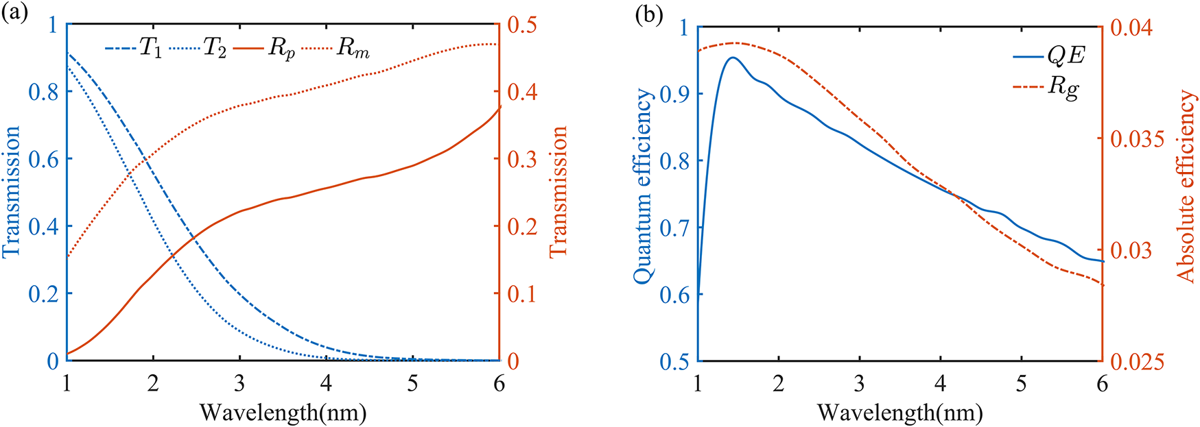
The efficiencies of the spectrometer’s components. (a) The dash-dot blue line is the transmission of 0.5 μm Al ${T}_1\left(\lambda \right)$
, the dotted blue line is the transmission of 0.75 μm Al
${T}_1\left(\lambda \right)$
, the dotted blue line is the transmission of 0.75 μm Al ${T}_2\left(\lambda \right)$
, the dotted brown line is the reflectivity of the plane mirror
${T}_2\left(\lambda \right)$
, the dotted brown line is the reflectivity of the plane mirror ${R}_\mathrm{p}\left(\lambda \right)$
and the solid brown line is the reflectivity of the toroidal mirror
${R}_\mathrm{p}\left(\lambda \right)$
and the solid brown line is the reflectivity of the toroidal mirror ${R}_\mathrm{m}\left(\lambda \right)$
. (b) The solid blue line is the quantum efficiency of the CCD
${R}_\mathrm{m}\left(\lambda \right)$
. (b) The solid blue line is the quantum efficiency of the CCD $\mathrm{QE}\left(\lambda \right)$
and the dash-dot brown line is the absolute efficiency of the grating
$\mathrm{QE}\left(\lambda \right)$
and the dash-dot brown line is the absolute efficiency of the grating ${R}_\mathrm{g}\left(\lambda \right)$
.
${R}_\mathrm{g}\left(\lambda \right)$
.

Measured spectral lines and the corresponding atomic structure information.

aNIST, National Institute of Standards and Technology.
Appendix A: The spectrometer parameters
The related efficiencies can be obtained at the beginning of the spectrometer design, as shown in Figure 9, including the reflection efficiency of the plane mirror ${R}_\mathrm{p}\left(\lambda \right)$
and the toroidal mirror
${R}_\mathrm{p}\left(\lambda \right)$
and the toroidal mirror ${R}_{\mathrm{m}}\left(\lambda \right)$
, the transmittance of the aluminum (Al) film
${R}_{\mathrm{m}}\left(\lambda \right)$
, the transmittance of the aluminum (Al) film $T\left(\lambda \right)$
and the diffraction efficiency of the grating
$T\left(\lambda \right)$
and the diffraction efficiency of the grating ${R}_\mathrm{g}\left(\lambda \right)$
. The charge-coupled device (CCD) used to record the number of photoelectrons
${R}_\mathrm{g}\left(\lambda \right)$
. The charge-coupled device (CCD) used to record the number of photoelectrons ${N}_\mathrm{pe}$
is an Andor Newton DO940P series. Its quantum detection efficiency
${N}_\mathrm{pe}$
is an Andor Newton DO940P series. Its quantum detection efficiency $\mathrm{QE}\left(\lambda \right)$
and the conversion relationship
$\mathrm{QE}\left(\lambda \right)$
and the conversion relationship $\eta \left(\lambda \right)$
between the number of photoelectrons and X-ray photons of different energies are also shown. The absolute number of photons emitted by the plasma can then be calculated as follows:
$\eta \left(\lambda \right)$
between the number of photoelectrons and X-ray photons of different energies are also shown. The absolute number of photons emitted by the plasma can then be calculated as follows:
 $$N=\frac{N_{\mathrm{p}\mathrm{e}}}{\mathrm{QE}\left(\lambda \right)\cdot \eta \left(\lambda \right)\cdot {R}_\mathrm{p}\left(\lambda \right)\cdot {R}_\mathrm{m}\left(\lambda \right)\cdot {R}_\mathrm{g}\left(\lambda \right)\cdot T\left(\lambda \right)}.$$
Based on the absolute number of photons, the absolute intensity of radiation emission $I\left(\lambda \right)$
from the plasma is deduced from the spectral emissivity per unit time, per unit area, per unit solid angle and per unit wavelength for specific wavelengths:
$I\left(\lambda \right)$
from the plasma is deduced from the spectral emissivity per unit time, per unit area, per unit solid angle and per unit wavelength for specific wavelengths:
 $$I\left(\lambda \right)=\frac{N\cdot hv}{\varOmega_{\mathrm{FFS}}\cdot \varDelta t\cdot S\cdot \varDelta \lambda},$$
where ${\varOmega}_{\mathrm{FFS}}$
is the solid acceptance angle of the spectrometer,
${\varOmega}_{\mathrm{FFS}}$
is the solid acceptance angle of the spectrometer, $\varDelta t$
is the emission time of the matter under investigation,
$\varDelta t$
is the emission time of the matter under investigation, $S$
is the surface area of the measured material,
$S$
is the surface area of the measured material, $\varDelta \lambda$
is the wavelength interval and
$\varDelta \lambda$
is the wavelength interval and $hv$
is the energy of a single photon.
$hv$
is the energy of a single photon.
Appendix B: The atomic structure information
In the analysis, the plasma is approximated as optically thin for the related lines and in the local thermodynamic equilibrium (LTE)[
Reference Aguilera and Aragón36]. In the case with carbon’s Ly β, Ly γ and He β lines, the limited spectral resolution of the spectrometer only allows the measurement of a blended peak intensity. For example, the line peak H-
$\beta$
actually contains two transitions $1\mathrm{s}\;{{}^2\mathrm{S}}_{1/2}\hbox{---} 3\mathrm{p}\;{{}^2\mathrm{P}}_{3/2}$
and
$1\mathrm{s}\;{{}^2\mathrm{S}}_{1/2}\hbox{---} 3\mathrm{p}\;{{}^2\mathrm{P}}_{3/2}$
and $1\mathrm{s}\;{{}^2\mathrm{S}}_{1/2}\hbox{---} 3\mathrm{p}\;{{}^2\mathrm{P}}_{1/2}$
, corresponding to
$1\mathrm{s}\;{{}^2\mathrm{S}}_{1/2}\hbox{---} 3\mathrm{p}\;{{}^2\mathrm{P}}_{1/2}$
, corresponding to ${\lambda}_{\mathrm{Ly}\hbox{-} \alpha 1}=2.84651\;\mathrm{nm}$
and
${\lambda}_{\mathrm{Ly}\hbox{-} \alpha 1}=2.84651\;\mathrm{nm}$
and ${\lambda}_{\mathrm{Ly}\hbox{-} \alpha 2}=2.84663\;\mathrm{nm}$
, respectively. Their relative intensity ratio can be calculated based on the data in Table 2.
${\lambda}_{\mathrm{Ly}\hbox{-} \alpha 2}=2.84663\;\mathrm{nm}$
, respectively. Their relative intensity ratio can be calculated based on the data in Table 2.
Appendix C: The density and temperature slices of the simulation
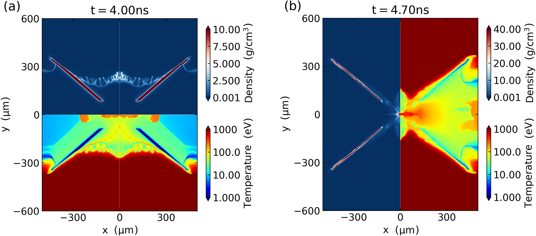
Figure 10 shows the density and temperature slices of the simulation at early time ( $t=4.0\;\mathrm{ns}$
) and collision time (
$t=4.0\;\mathrm{ns}$
) and collision time ( $t=4.7\;\mathrm{ns}$
). Our target and laser pulse shape are the same as in the experiment. The CD plasma is compressed in the cones and collides at the spherical center. Since the Mach number of the compressed plasma is approximately 4[
Reference Liu, Wu, Zhang, Yuan, Zhang, Xu, Xue, Tian, Zhong and Zhang37], a strong shock is launched at the collision region and propagates outwards. The shock would dissipate the kinetic energy of the plasma and convert it to internal energy to reach a high temperature in the shocked region (∼550 eV). This temperature is a little higher than the measured core temperature of a Kirkpatrick–Baez (KB) microscope (340–390 eV) with the same nanosecond laser energy[
Reference Fang, Zhang, Dong, Zhang, Zhang, Yuan, Li and Zhang11]. Our simulated peak density of shocked CD plasma is roughly 37 g cm–3, lower than the detected density (
$t=4.7\;\mathrm{ns}$
). Our target and laser pulse shape are the same as in the experiment. The CD plasma is compressed in the cones and collides at the spherical center. Since the Mach number of the compressed plasma is approximately 4[
Reference Liu, Wu, Zhang, Yuan, Zhang, Xu, Xue, Tian, Zhong and Zhang37], a strong shock is launched at the collision region and propagates outwards. The shock would dissipate the kinetic energy of the plasma and convert it to internal energy to reach a high temperature in the shocked region (∼550 eV). This temperature is a little higher than the measured core temperature of a Kirkpatrick–Baez (KB) microscope (340–390 eV) with the same nanosecond laser energy[
Reference Fang, Zhang, Dong, Zhang, Zhang, Yuan, Li and Zhang11]. Our simulated peak density of shocked CD plasma is roughly 37 g cm–3, lower than the detected density ( $46\pm 24\;\mathrm{g}\;{\mathrm{cm}}^{-3}$
)[
Reference Zhang, Yuan, Zhang, Liu, Fang, Zhang, Liu, Zhao, Dong, Liu, Dai, Gu, Li, Zheng, Zhong and Zhang12], and well above
$46\pm 24\;\mathrm{g}\;{\mathrm{cm}}^{-3}$
)[
Reference Zhang, Yuan, Zhang, Liu, Fang, Zhang, Liu, Zhao, Dong, Liu, Dai, Gu, Li, Zheng, Zhong and Zhang12], and well above ${10}^{24}\;{\mathrm{cm}}^{-3}$
as indicated by the absence of spectral lines.
${10}^{24}\;{\mathrm{cm}}^{-3}$
as indicated by the absence of spectral lines.
Density and electron temperature slices of the FLASH simulation at (a) early time ( $t=4.0\;\mathrm{ns}$
) and (b) collision time (
$t=4.0\;\mathrm{ns}$
) and (b) collision time ( $t=4.7\;\mathrm{ns}$
).
$t=4.7\;\mathrm{ns}$
).

Acknowledgements
This work is supported by the Strategic Priority Research Program of the Chinese Academy of Sciences (Grant Nos. XDA25030300, XDA25051200 and XDA25010100), the Natural Science Foundation of Shandong Province (Grant No. ZR2019ZD44) and the National Natural Science Foundation of China (Grant Nos. 12034020 and 12205185).








 Open access

