OBSERVATIONAL CONSTRAINTS AND MODEL MOTIVATION

Observations indicate that a rising ocean tide causes grounding line retreat and lifts the ice shelf away from sub-shelf bathymetric pinning points, decreasing resistance to the flow of the ice shelf (Schmeltz and others, Reference Schmeltz, Rignot and MacAyeal2001; Doake and others, Reference Doake2002; Minchew and others, Reference Minchew, Simons, Riel and Milillo2017). Conversely, a rising tide also increases hydrostatic stresses in the ice shelf, which increases the resistance to ice flow (e.g. Anandakrishnan and Alley, Reference Anandakrishnan and Alley1997; Gudmundsson, Reference Gudmundsson2007; Rosier and Gudmundsson, Reference Rosier and Gudmundsson2016). In this section, we analyze observations of tidally-modulated ice shelf flow variations at two West Antarctic ice streams and discuss which physical processes might play a role in causing these variations.

At RIS, horizontal ice shelf displacement (blue line in Fig. 1a) varies primarily at fortnightly periods, with smaller semidiurnal variations in displacement that are nearly in phase with tidal height (calculated to be 15° phase lag, though not necessarily discernible in Fig. 1a). At BIS (Fig. 1b), horizontal ice displacement varies at fortnightly and diurnal periods with nearly equal amplitude, with diurnal variations completely out of phase with tidal height (210° phase lag). At both ice streams, there is a significant low-frequency signal in horizontal displacement downstream of the grounding line. However, the variations in displacement occurring at high tidal frequencies have different phase with respect to tidal height. We aim to explain the causes of these similarities and differences between the tidally-induced ice shelf flow variations at these two ice streams.

Fig. 1.

Observations and model simulations of the tidal response to forcing near and downstream from the grounding lines of two ice streams. (a) Blue line is detrended horizontal along-flow displacement measured at a GPS station downstream of RIS grounding line over one spring-neap cycle (R-20 in Gudmundsson, Reference Gudmundsson2006, coordinates in Table 1). Red line is detrended vertical displacement measured at this same station. Data from Gudmundsson (Reference Gudmundsson2006). (b) Same as (a), but for GPS station downstream of BIS grounding line (DFLT station in Brunt and others, Reference Brunt, King, Fricker and MacAyeal2010, coordinates in Table 1). Data from personal communication with R. Bindschadler and K. Brunt. (c) Relationship between strain (y-axis) and tidal height (x-axis) just downstream of the RIS grounding line. Grey dots indicate GPS observations. Strain is calculated between the R-20 station, which is 20 km downstream of the grounding line of RIS and the R + 00 station, which is on the time-averaged RIS grounding line (as named in Gudmundsson, Reference Gudmundsson2006). Tidal height is measured at the R-20 station on the ice shelf. Solid black line indicates the least squares estimate, written in functional form in the inset box. Dashed black lines indicate the two standard deviation estimates for least-squares parameters (with exponent α = 1.54 ± 0.06). Measurements of detrended displacement more than two standard deviations different from the mean are removed, followed by smoothing with a 30-minute Gaussian filter. (d) Same as (c), but for strain calculated between the DFLT station, ~15 km downstream of the BIS grounding line, and the D010 station, ~10 km upstream of the time-averaged BIS grounding line (as named in Brunt and others, Reference Brunt, King, Fricker and MacAyeal2010, with exponent α = 2.53 ± 0.19). Greater measurement error at RIS causes the larger spread in intercept of least squares estimates. (e) Simulated ice shelf flow in a simple viscoelastic model (Eqns (4)–(10)) for a Rutford-like parameter set. Blue line is detrended horizontal displacement and red line is tidal height, as in panels (a, b). In the model, strain is calculated and then integrated over a horizontal length scale corresponding to the distance between GPS stations on an ice stream, 20 km in the case of RIS and 25 km in the case of BIS. (f) Same as in (e), but for a Bindschadler-like parameter set.

Table 1.

Locations of GPS stations (at beginning of observation period of data used in this study) referenced in text and used to calculate ice shelf flow in Fig. 1

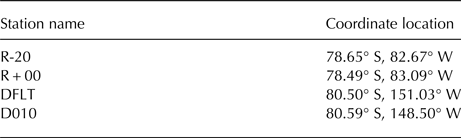
Data from Gudmundsson (Reference Gudmundsson2006) and personal communication from R. Bindschadler and K. Brunt.

We first discuss different ways in which tides cause variations in the stress applied on an ice shelf. To do so, we analyze observations of the relationship between horizontal strain and tidal height at RIS and BIS (Figs. 1c and d, respectively). Strain is measured over a baseline distance between stations near and downstream of the grounding lines of RIS and BIS (with the understanding that ice stream grounding line locations vary with tidal height and measurements of grounding line position are subject to significant errors, see Rignot and others, Reference Rignot, Mouginot and Scheuchl2011). Observations are indicated by grey circles, and the least squares fit of the relationship between tidal height and ice shelf strain is indicated by the black solid line (black dashed lines indicate the ±2σ least squares fits), with the functional form written explicitly in the inset boxes. For elastic deformations, strain is proportional to the imposed stress. If viscous deformation is small compared with elastic deformation, then the phase of high-frequency variations in observed strain with respect to tidal height are expected to be close to either 0° or 180° (see the section ‘Parameter exploration of tidal influence on ice shelf flow’, below). In such a scenario, measured variations in strain can be used as indicators of variations in stress. In the floating portion of RIS (Fig. 1c), strain is positively correlated (close to 0° in phase) and nonlinear with respect to tidal height. This nonlinearity indicates that strain is more sensitive to changing tides at high tide than at low tide. In contrast, strain in the floating portion of BIS (Fig. 1d) is negatively correlated (close to 180° out of phase) and nonlinear with respect to tidal height, with higher sensitivity to changing tides at low tide.

Variations in hydrostatic (and flexural) stresses within an ice shelf are linearly proportional to local tidal height (Holdsworth, Reference Holdsworth1969; Anandakrishnan and Alley, Reference Anandakrishnan and Alley1997; Gudmundsson, Reference Gudmundsson2007; Rosier and Gudmundsson, Reference Rosier and Gudmundsson2016). Thus, our primary goal in this study is to determine mechanisms which can plausibly produce the observed nonlinear relationships between ice shelf strain and tidal height in the ice shelves at RIS and BIS. Spatially-resolved InSAR observations indicate that these tidal strain variations are localized in nature (Minchew and others, Reference Minchew, Simons, Riel and Milillo2017), suggesting that the mechanism causing ice shelf flow variations is unrelated to large-scale processes including either changes in ice shelf slopes and driving stresses (Makinson and others, Reference Makinson, King, Nicholls and Hilmar Gudmundsson2012) or changes in the velocity of the grounded ice stream, which advect downstream to the ice shelf (Gudmundsson, Reference Gudmundsson2011). We argue that beyond hydrostatic, flexural and driving stresses, the only way for tides to cause localized variations in ice shelf strain is through variations in resistance from localized contact at the lower and lateral ice shelf surfaces. The total of the stresses exerted back on the grounded ice stream by all different contact points on these pinned ice shelf surfaces is typically referred to as the ‘buttressing stress’ (Goldberg and others, Reference Goldberg, Holland and Schoof2009).

We consider the locations of ‘final contact points’ where ice goes afloat and loses contact with the bed because the weight of ice is approximately equal (or exactly equal in the hydrostatic limit) to the hydrostatic pressure of ocean water. These final contact points occur at (what is conventionally called) the grounding line, and also at pinning points within the ice shelf where local maxima in bathymetry come into contact with the lower ice shelf surface (see schematic example in Fig. 2). Tidal variations in hydrostatic pressure lead to migration of these final contact points and change the total area where ice-bed contact occurs (as previously argued by Anandakrishnan and Alley, Reference Anandakrishnan and Alley1997). By simply considering where hydrostatic equilibrium occurs near the grounding line and in ice shelves, it has been shown (Tsai and Gudmundsson, Reference Tsai and Gudmundsson2015) that final contact points (either a grounding line or pinning point) migrate ~10 times further upstream from mean to high tide than from low to mean tide. This asymmetry arises because spatial variations in ice thickness are set by slow viscous deformation of the ice sheet. However, on the typical timescale of tidal hydrostatic pressure variations (12–24 h), viscous deformation is too slow to adjust ice thickness in the vicinity of the final contact points in response to the accumulation of hydrostatic stresses.

Fig. 2.

Explanatory schematic for the mechanisms of tidal modulation of ice shelf buttressing stresses. Tides modulate the location of ice contact with the bed, which occurs at the grounding line and sub-shelf pinning points. The migration of the grounding line and pinning point locations is asymmetric with respect to tidal height (Tsai and Gudmundsson, Reference Tsai and Gudmundsson2015). Colored lines are positions of ice shelf at different location in the tidal cycle: red is low tide, black dashed is mean tide and blue is high tide. Black triangles correspond to two GPS stations, which would record the change in ice shelf horizontal strain with changing tidal height.

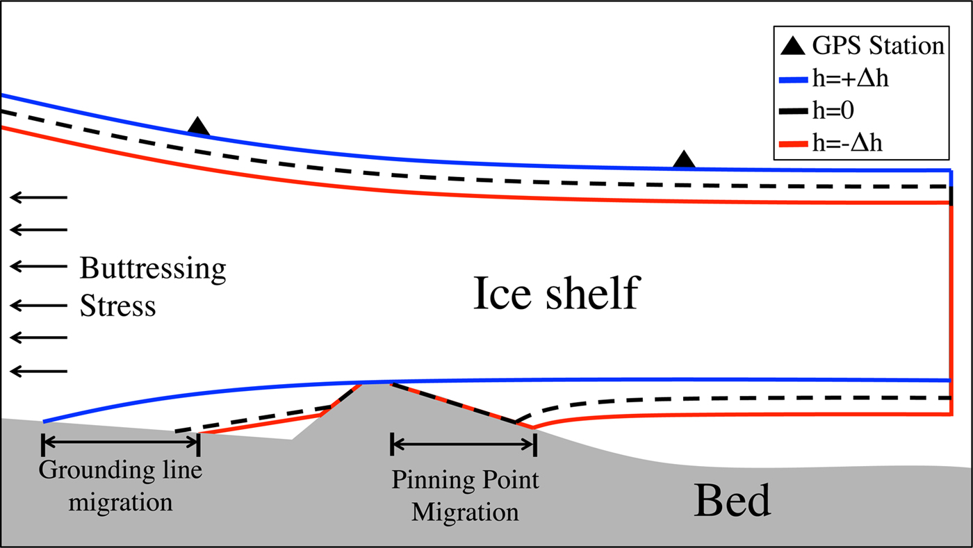
An explanatory schematic (Fig. 2) shows the asymmetric migration of the grounding line and a pinning point from low to mean to high tide. The precise functional dependence of the total contact area on tidal height will depend on the particulars of local bathymetry. However, if there is non-zero basal shear stress that is approximately spatially uniform over all locations of ice contact, the decrease in the spatially-integrated basal shear stress associated with grounding line retreat will be greater in going from mean to high tide than from low to mean tide. The consequence of this asymmetry is a nonlinear relationship between tidal height and the total buttressing stress within the ice shelf. Indeed, at at both RIS and BIS, ice shelf strain is a nonlinear function of tidal height (Figs. 1c and d). To capture this asymmetry, we formulate (in the next section) a very general empirical parameterization for total ice shelf buttressing stress as an increasing function of tidal height with arbitrary shape. We then use observations of the relationship between tidal height and ice shelf strain (e.g. Figs. 1c and d) to constrain the shape of this function, and explore the consequences of this nonlinearity on the observed ice shelf strain using a lumped viscoelastic ice shelf model.

VISCOELASTIC ICE SHELF MODEL

To determine the relative importance of variations in hydrostatic and buttressing stresses in generating the period, phase and amplitude of observed ice shelf flow variability, we use a lumped viscoelastic model. For simplicity, the normalized tidal height is assumed to be composed of two high-frequency components of equal amplitude

(1) $$\hat h(t) = \displaystyle{1 \over 2}(\sin \omega _{h1} t + \sin \omega _{h2} t).$$

By only forcing the model at high frequencies, we can isolate the effect of nonlinearities in the ice shelf dynamics in producing a low-frequency ice shelf response. Also, in reality, high-frequency tidal constituents may have different amplitudes. Regardless, simulations forced directly by tidal heights observed in ice shelves of interest (e.g. red lines in Figs.1a and 1b) do not produce a qualitatively different ice flow response than simulations forced by the simpler tidal height in Eqn (1).

Considering the ice shelf as a simple elastic beam, tidal variations in water level will cause stress variations within the ice shelf through hydrostatic pressure and ice flexure. Changes in hydrostatic stresses within the ice shelf are proportional to tidal height

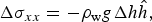(2) $$\Delta \sigma _{xx} = - \rho _{\rm w} g\Delta h\hat h,$$

where Δh is the tidal range, ρ _w is the density of ocean water, g is the acceleration due to gravity and negative values denote horizontal compression of the ice shelf (Rosier and others, Reference Rosier, Gudmundsson and Green2014). Changes in longitudinal stress associated with ice shelf flexure at the lower ice surface around a non-migrating grounding line are proportional to tidal height

(3) $$\Delta \sigma _{xx} (z = 0) \propto - \Delta h\hat he^{ - L_x x} \left( {\cos L_x x - \sin L_x x} \right),$$

where $L_x^{ - 1} $ is a flexure length scale dependent on ice shelf rheology (Holdsworth, Reference Holdsworth1969). However, flexural stresses quickly drop off within the ice shelf (Rosier and Gudmundsson, Reference Rosier and Gudmundsson2016), and average to zero when integrated over the ice shelf thickness. Since we consider such a depth-integrated, lumped representation of an ice shelf in this study, flexural stresses are negligible and thus we only consider hydrostatic stresses,

(4) $$\sigma _h = - \sigma _{h0} \hat h,$$

where σ _h0 is the magnitude of tidal variations in hydrostatic stress within the ice shelf, which cause compression of the ice shelf at high tide and extension of the ice shelf at low tide.

Downstream of the grounding lines of RIS and BIS, measured ice shelf strain varies nonlinearly with tidal height (Fig. 1), likely as a consequence of tidal asymmetries in grounding line migration and the contact between the ice shelf and sub-shelf bathymetry (as discussed in the section ‘Observational constraints and model motivation’). Thus, we can use the shape of the measured relationship between ice shelf strain and tidal height, captured by the (black line) nonlinear least squares estimates in Figs. 1c and d, as an empirical measure of the shape of this asymmetry. The equivalent buttressing stress (which as we argue above, is proportional to strain for elastic deformations) is parameterized as an increasing function with arbitrary shape

(5) $$\sigma _b = \beta \sigma _{h0} \left[ {2^{1 - \alpha} (1 + \hat h)^\alpha - 1} \right],$$

where α is a shape parameter indicating the strength of the asymmetry in buttressing stress with respect to tidal height (the same shape parameter that is fit in Figs. 1c and d), and

(6) $$\beta = \displaystyle{{\sigma _{b0}} \over {\sigma _{h0}}}, $$

is a non-dimensional parameter measuring the relative importance of the magnitude of changes in buttressing stress (σ _b0) to the magnitude of changes in hydrostatic stress (σ _h0). The value of β cannot be determined strictly from the strain/height relationship in Figs. 1c and d, since measured strains include the effect of hydrostatic stress variations. The bracketed term in Eqn (5) varies between −1 to 1 regardless of the value chosen for α. It should be noted that this parameterized buttressing equation could just as easily have taken other forms, such as a polynomial. Here, we choose this particular functional form of Eqn (5) in order to easily parameterize the magnitude (β) and shape (α) of buttressing stress variations with a minimum of parameters and without introducing other potential sources of nonlinearity or asymmetry with respect to tidal height. It is not necessarily the case that the buttressing relationship will be nonlinear (as this form permits the possibility that α = 1), but rather, we use the observations of nonlinearities in ice shelf strain as a guide for setting the value of α. In the section ‘Parameter exploration of tidal influence on ice shelf flow’, we further explore the sensitivity of the modeled ice flow response to the values of α and β.

We simulate the tidal variations in local ice shelf deformation using a lumped Maxwell model (Tsai and others, Reference Tsai, Rice and Fahnestock2008) for a viscoelastic beam unconfined in the y and z direction and driven by tidal variations in stress in the x direction

(7) $${\rm \varepsilon} _{xx} = \displaystyle{1 \over E}(\sigma _{\rm b} + \sigma _{\rm h} ) + \int_0^t \displaystyle{1 \over {3\eta _e}} (\sigma _{\rm b} + \sigma _{\rm h} ){\rm d}t,$$

where ε _xx is the longitudinal strain, E is the Young's modulus of ice and η _e is the effective viscosity within the ice shelf (MacAyeal and others, Reference MacAyeal, Sergienko and Banwell2015). The model is ‘lumped’ in that it is forced by the average stresses in a section of the ice stream that includes the grounding line and some part of the ice shelf. The effective viscosity in this section of the ice stream is a function of the time-averaged (indicated by overbar) second invariant of the deviatoric stress tensor

(8) $$\bar I_2 = \displaystyle{1 \over 2}(\bar \sigma _{xx}^2 + \bar \sigma _{yy}^2 + \bar \sigma _{zz}^2 ) + \bar \sigma _{xy}^2 + \bar \sigma _{xz}^2 + \bar \sigma _{yz}^2, $$

where we expect that the longitudinal and lateral shear stresses will dominate for ice shelves (as in Goldberg and others, Reference Goldberg, Schoof and Sergienko2014). We separate tidally-driven variations in hydrostatic (σ _h) and buttressing stresses (σ _b) from the sum of the squares of the time-averaged deviatoric stresses ( $\bar I_2 $ ,) giving an effective viscosity

(9) $$\eqalign{\eta _{\rm e} = & \displaystyle{1 \over 2}A^{ - 1} \left[ {\displaystyle{1 \over 2}\sigma _{\rm b} (t)^2 + \displaystyle{1 \over 2}\sigma _{\rm h} (t)^2 + \bar I_2} \right]^{\textstyle{{1 - n} \over 2}} \cr = & \displaystyle{1 \over 2}A^{ - 1} \sigma _{h0}^{1 - n} \left[ {\displaystyle{{\beta ^2} \over 2}\left[ {2^{1 - \alpha} (\hat h + 1)^\alpha - 1} \right]^2 + \displaystyle{{\hat h^2} \over 2} + \gamma ^2} \right]^{\textstyle{{1 - n} \over 2}},} $$

where A and n are the rate factor and exponent in the Nye–Glen constitutive law (Cuffey and Paterson, Reference Cuffey and Paterson2010), respectively, and

(10) $$\gamma ^2 = \displaystyle{{\bar I_2} \over {\sigma _{h0}^2}} $$

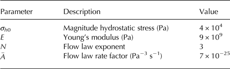
is a non-dimensional parameter measuring the relative importance of the magnitude of total time-averaged stresses in the ice shelf (such as driving and lateral shear stresses, which determine the time-averaged ice flow) to the magnitude of tidal variations in hydrostatic stress. The driving and other background stresses within the ice shelf are only included in the effective viscosity and nowhere else in the Maxwell model, as we intend to simulate the tidal anomalies in ice shelf deformation, but not the time-averaged ice flow. We choose to separate tidally-varying from time-averaged terms in the effective viscosity in order to simplify the effective viscosity terms, but this choice has no significant quantitative effect on the results discussed hereafter. The parameterizations and the lumped nature of this viscoelastic model enable straightforward parameter exploration, but would be made unnecessary by a fully 3-D viscoelastic ice-stream model with realistic sub-shelf bathymetry. However, the bathymetry and many other parameters that would be required for such a model are generally poorly constrained. We therefore leave such a modeling approach to future studies (Table 2).

Table 2.

Parameters used in lumped Maxwell ice shelf model (as described in the section ‘Viscoelastic ice shelf model’) unless otherwise indicated in text

MODELED TIDAL ICE FLOW VARIATIONS AT RUTFORD AND BINDSCHADLER ICE STREAMS

The lumped Maxwell model we have described can explain why glaciers respond differently to tides. In this section, we focus on the two cases of RIS and BIS where the phase, amplitude and period of tidally-driven ice flow variations are considerably different. We use the lumped Maxwell model to calculate the detrended displacement calculated for parameter regimes similar to these two cases. We have plotted the results in Figs. 1e and f for easy comparison with observations (Figs. 1a and b).

In a Rutford-like case (Fig. 1e, with α = 1.54, β = 1.4 and γ = 2.9), the ice shelf is forced by tidal variation at M ₂ and S ₂ periods, with hydrostatic stress variations of 55 kPa amplitude (consistent with combined M ₂ and S ₂ tidal height variations of ~6 m). In this case, β > 1 and γ is large, corresponding to a situation where changes in hydrostatic stresses are smaller than changes in both buttressing stresses and background stresses in the ice shelf. Variations in simulated displacement are nearly in phase with semidiurnal variations in tidal height. These semidiurnal variations in displacement are smaller in amplitude than the dominant low-frequency signal at the M _sf tidal period, which arises from the buttressing nonlinearity (as α > 1 in this case). We can understand this low-frequency ice-stream response by noting that a nonlinear power of the tidal height as it appears in Eqn (5) can be expanded as

(11) $$(1 + \hat h)^\alpha = 1 + \alpha \hat h + \displaystyle{{\alpha (\alpha - 1)} \over 2}\hat h^2 + \ldots $$

(12) $$\eqalign{ = 1 \,+&\; \displaystyle{\alpha \over 2}\left[ {\sin (\omega _{h1} t) + \sin (\omega _{h2} t)} \right] + \displaystyle{{\alpha (\alpha - 1)} \over 8}[ {\mathop {\sin} \nolimits^2 (\omega _{h1} t) }\cr +&\; {\mathop {\sin} \nolimits^2 (\omega _{h2} t) + 2\sin (\omega _{h1} t)\sin (\omega _{h2} t)}] + \ldots,} $$

which can be rewritten using the double angle and product to sum of sinusoidal functions

(13) $$\eqalign{(1 + \hat h)^\alpha &= 1 + \displaystyle{\alpha \over 2}\left[ {\sin (\omega _{h1} t) + \sin (\omega _{h2} t)} \right] + \displaystyle{{\alpha (\alpha - 1)} \over 8} \cr &\quad \times \left[ 1 - \displaystyle{1 \over 2}\cos (2\omega _{h1} t) - \displaystyle{1 \over 2}\cos (2\omega _{h2} t) \right. \cr &\quad \left. \vphantom{1 - \displaystyle{1 \over 2}\cos (2\omega _{h1} t) - \displaystyle{1 \over 2}\cos (2\omega _{h2} t)} + \cos \left( {(\omega _{h1} - \omega _{h2} )t} \right) - \cos \left( {(\omega _{h1} + \omega _{h2} )t} \right) \right] + \ldots} $$

which includes power at a low beat frequency ω _L  = ω _h1 − ω _h2. The ‘frequency mixing’ of Eqn (13) is a mathematical property of any system with nonlinearities, which is forced at more than one frequency. In this case, the nonlinearity arises through processes occurring in the ice shelf. By providing a nonlinear mechanism that produces a low-frequency ice flow response in the ice shelf, we can explain InSAR observations that show that the low-frequency signal at RIS originates in the ice shelf (Minchew and others, Reference Minchew, Simons, Riel and Milillo2017). More broadly, with these parameters, the model quantitatively reproduces the characteristic phase, amplitude and frequency of observed flow variations in the ice shelf downstream of RIS (Fig. 1a).

In a Bindschadler-like case (Fig. 1f, with α = 2.53, β = 0.3 and γ = 4), the ice shelf is forced by tidal variation at O ₁ (25.92 h) and K ₁ (24.00 h) periods, with hydrostatic stress variations of 30 kPa amplitude (consistent with combined O ₁ and K ₁ tidal height variations of ~3.2 meters). In this case, β < 1 and γ is large, indicating a scenario where changes in hydrostatic stresses are large compared with changes in buttressing stresses and small compared with background stresses in the ice shelf. Consequently, diurnal variations in horizontal displacement are close to 180° out of phase with the prescribed diurnal variations in tidal height. Although the dominant variations in hydrostatic stress are linear with tidal height, nonlinear changes in buttressing stresses (α > 1 also in this case) and effective viscosity are sufficiently important to introduce a significant low-frequency component into the tidal response that is comparable with the amplitude of the diurnal response. This case quantitatively reproduces the phase, amplitude and frequency of ice flow variations at BIS, which are close to 180° out of phase with tidal height and comparable in amplitude with the low-frequency response (Fig. 1b).

Comparison of the two cases of RIS and BIS shows that even though the dominant tidal periods in the Weddell and Ross Seas are quite different, the existence of an asymmetry in buttressing stresses with respect to tidal height produces an ice stream response that includes variation on long spring-neap timescales for both ice streams. However, there are also important differences in the flow response of BIS and RIS. In particular, there are significant differences in the phasing of the high-frequency ice shelf flow response relative to the dominant tidal forcing and the amplitude of the high-frequency ice shelf flow response relative to the low-frequency flow response.

PARAMETER EXPLORATION OF TIDAL INFLUENCE ON ICE SHELF FLOW

In this section, we systematically explore the parameter space of the lumped Maxwell model. We explore how the high-frequency phase and dominant period of the modeled variations in ice shelf displacement are functions of parameters α, β and γ. We show that it is the relative importance of tidal variations in hydrostatic and buttressing stresses (β in Eqn (5)), and to a lesser extent the strength of the viscous ice shelf response to tides (γ in Eqn (9)), that cause differences in the tidally-driven ice flow variation at different ice streams. We start by analyzing the phase of high-frequency variations in horizontal ice displacement with respect to tidal height, as a function of β and γ (Figs. 3a and b) for two values of α that are similar to those for RIS and BIS (see Figs. 1c and d). When β < 1, changes in hydrostatic stresses dominate changes in buttressing stresses and displacement is close to 180° out of phase with tidal height. Conversely, when β > 1, changes in buttressing stresses dominate and the displacement is nearly in phase with tidal height. There is a sharp transition between these two regimes at β = 1, suggesting that the observed phase lag between high-frequency variations in ice displacement and tidal height (and whether it is near 0° or 180°) is a strong indicator of whether hydrostatic stress variations or buttressing stress variations dominate the tidal modulation of ice shelf flow. Furthermore, increasing γ decreases the effective viscosity, therefore increasing the amplitude of the viscous deformation response to forcing, leading to an increase in the phase lag of horizontal displacement with respect to tidal forcing.

Fig. 3.

Parameter space exploration of the response of ice shelf displacement to tidal forcing in the viscoelastic ice shelf model. All panels include variations in β, the ratio of changes in buttressing stress to hydrostatic stress, on the x-axis and γ, the ratio of time-averaged background stresses in the ice shelf to variations in hydrostatic stress, on the y-axis. Black circles indicate parameter set associated with Rutford-like simulation plotted in Fig. 1e. (a, b) Phase lag of M ₂ component of detrended ice shelf displacement with respect to tidal height. (c, d) Difference between the log of power spectral density (S) of detrended horizontal ice displacement at low frequencies (M _sf) and high frequencies (M ₂) of tidal forcing. White shading indicates equal power at low and high frequencies.

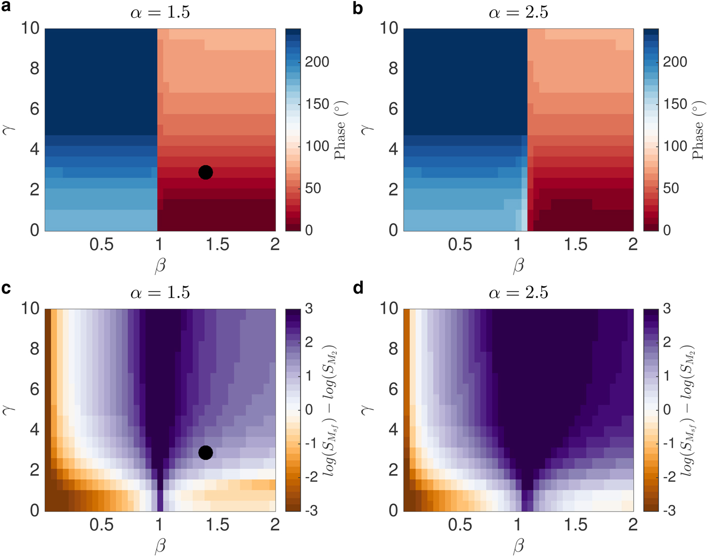
To determine the dominant timescale of the ice shelf response to tides, we examine (Figs. 3c and d) the difference between the logarithm of power spectral density (S) for detrended horizontal ice displacement at low frequencies (M _sf) and the high frequencies of tidal forcing (M ₂ and S ₂ in Fig. 3), as a function of β and γ for the same two values of α as in Figs. 3a and b. Where values are large, the low-frequency response of ice flow to tidal forcing dominates over the high-frequency ice flow response (at the same frequency as the forcing). Changes in γ cause two opposite effects in the ice flow response to tidal forcing. When γ increases, the time-averaged deviatoric stresses in the nonlinear effective viscosity ( $\bar I_2 $ in Eqn (9)) become larger relative to the tidally-varying terms (σ _h and σ _b). The result is that tidal forcing causes proportionately less change in effective viscosity and the nonlinearity of effective viscosity in the Nye-Glen flow law for ice becomes less important. In addition, increasing γ decreases the overall magnitude of effective viscosity (through the dependence of viscosity on deviatoric stresses in ice, see Eqn (9)). When the ice shelf strain varies on periods longer than the Maxwell time (the characteristic relaxation timescale for a Maxwell material: τ _m = η _e/E), the corresponding deformation will primarily be viscous. At lower viscosity, the amplitude of the resulting variations in viscous deformation will be larger, while the high-frequency elastic deformations are largely unchanged (Lakes, Reference Lakes1998). Consequently, this second effect leads to an increase in the amplitude of low-frequency variations in ice flow relative to high-frequency variations with increasing γ. Figs. 3c and d show that in a range of parameters relevant to ice shelves, increasing γ generally leads to an increase in the amplitude of low-frequency components relative to high-frequency components. Thus, we conclude that the second effect is generally more important than the first, except when α and γ are low and β is very high (like in the bottom right corner of Fig. 3c). We also find that, even when the magnitude of linear changes in hydrostatic stresses dominate nonlinear changes in buttressing stresses (β < 1), low-frequency variations in ice flow can be significant (as long as γ is sufficiently large). Even in the Bindschadler-like case shown in Fig. 1f, there is a significant component of the variation in ice shelf flow occurring at M _sf periods.

As argued in the section ‘Modeled tidal ice flow variations at Rutford and Bindschadler ice streams’, when α ≠ 1, the nonlinearity in buttressing stress with respect to tidal height causes mixing of high-frequency forcings to produce a low-frequency response in ice flow. Thus, increasing α leads to an expansion in the range of parameter space over which the low-frequency ice-shelf response dominates (in Fig. 3, white regions demarcate where this ratio is near one). In the marginal case where variations in buttressing stresses are exactly linear with respect to tidal height (α = 1; not shown), we find that no amount of viscous nonlinearity is able to produce power at low frequencies. This lack of low-frequency response is similar to previous studies (Gudmundsson, Reference Gudmundsson2007, Reference Gudmundsson2011), which found that the nonlinearity of the Nye-Glen flow law is insufficient on its own to reproduce the low-frequency response of RIS to high-frequency tidal forcing. Other nonlinearities, which come from asymmetries in buttressing in our model (and sliding relations for grounded ice in other studies) are necessary, though not strictly sufficient, to produce a dominantly low-frequency response in horizontal ice displacement. Given that γ is large in most ice streams, we expect there generally to be some detectable ice flow variation at the tidal beat frequency if tides cause variations in ice shelf buttressing stress with magnitude greater than ~25% of the magnitude of hydrostatic stress variations (with the specific number depending on precise values of γ and α).