


1. Introduction
The aviation industry has made remarkable strides in addressing the multifaceted challenges associated with aircraft noise emissions. This persistent concern arises from the profound impact of aircraft noise emissions on both the environment and the communities surrounding airports. As air traffic continuously grows and noise regulations become more stringent, more significant reductions in aircraft noise emissions will be required. Traditionally, the aerospace community has predominantly focused on mitigating noise emissions originating from the propulsion system such as jet engines. However, advancements in turbofan technologies have substantially reduced engine-related noise and prompted a shift in research focus, with airframe noise also becoming a limiting factor in the overall noise reduction of aircraft, especially in its approach and landing configurations where the engines are throttled down (Peake & Parry Reference Peake and Parry2012). As a result, there has been an increased scientific interest in understanding and modelling the noise-generation mechanisms at landing gears and high-lift devices (e.g. flaps and slats) (Dobrzynski Reference Dobrzynski2010; Nicolas Reference Nicolas2019), which are identified as primary sources of airframe noise (Horne et al. Reference Horne, James, Arledge, Soderman, Burnside and Jaeger2005; Khorrami et al. Reference Khorrami, Lockard, Humphreys, Choudhari and Van de Ven2008).
Of various geometries studied, wing-tip noise has drawn considerable attention in academia and industry, since it is a key element in the study of more complex flow structures that are seen in modern aeroacoustic problems. For example, a wing-tip model has frequently been used to gain insights into the aeroacoustics of the flap side edge (McInerny, Meecham & Sodermant Reference McInerny, Meecham and Soderman1989; Rossignol Reference Rossignol2013; Giraldo et al. Reference Giraldo, Botero, Pereira, Catalano, Reis and Coelho2018) and fan blades with tip gap (Camussi et al. Reference Camussi, Grilliat, Caputi-Gennaro and Jacob2010; Decaix et al. Reference Decaix, Balarac, Dreyer, Farhat and Münch2015). Previous investigations employing experimental (Dobrzynski et al. Reference Dobrzynski, Nagakura, Gehlhar and Buschbaum1998; Guo Reference Guo1999; Guo & Joshi Reference Guo and Joshi2003; Yamamoto et al. Reference Yamamoto2018) and computational (Lockard et al. Reference Lockard, Choudhari, O’Connell, Duda and Fares2017) approaches have agreed that the flap side edge is a prominent contributor to aircraft high-lift noise. The noise from tip leakage flow on fan blades is also part of the broadband component that accounts for 50 % of the overall aircraft noise during the landing phase (Camussi et al. Reference Camussi, Grilliat, Caputi-Gennaro and Jacob2010). These studies show that the baseline flow topology for all these cases is common with that of the wing tip, comprised of a vortex system generated from the convective flow around the wing-tip geometry.
Among the flow features that exist at the wing-tip geometry, the most prominent and common one is the formation of a dual-vortex structure. This is a flow phenomenon extensively studied both numerically and experimentally for wing tip (McInerny et al. Reference McInerny, Meecham and Soderman1989; Rossignol Reference Rossignol2011; Imamura, Enomoto & Yamamoto Reference Imamura, Enomoto and Yamamoto2012; Giraldo et al. Reference Giraldo, Botero, Pereira, Catalano, Reis and Coelho2018) and flap side edge (Khorrami, Singer & Takallu Reference Khorrami, Singer and Takallu1997; Meadows et al. Reference Meadows, Brooks, Humphreys, Hunter and Gerhold1997; Radeztsky, Singer & Khorrami Reference Radeztsky, Singer and Khorrami1998; Khorrami & Singer Reference Khorrami and Singer1999; Khorrami, Singer & Radeztsky Reference Khorrami, Singer and Radeztsky1999; Choudhari et al. Reference Choudhari2002; Angland Reference Angland2008; Buffo et al. Reference Buffo, Wolf, Dufhaus, Hoernschemeyer and Stumpf2012; Casalino et al. Reference Casalino, Fares, Duda, Hazir and Khorrami2015). The formation of this flow structure is mainly driven by the pressure difference between the pressure and suction surfaces, which results in the separation of the spanwise crossflow along the corner between the pressure surface and the tip surface. The shear layer then rolls up to form the primary vortex. The outer flow reattaching on the tip surface results in the formation of a second shear layer at the suction surface edge, which rolls up to form the secondary vortex on the suction surface. The intensity of the circumferential velocity in these vortices is comparable to the freestream velocity (McAlister & Takahashi Reference McAlister and Takahashi1991). The two vortices grow in strength and size along the streamwise direction. Giuni & Green (Reference Giuni and Green2013) showed that for the NACA 0012 wing-tip geometry, the vortices grow from $x/c=0.2$
to
$x/c=0.2$
to $x/c=0.5$
. Eventually, the primary vortex ‘crosses over’ from the wing-tip surface to the suction surface, interacting and merging with the secondary vortex into a single dominant vortex (Khorrami & Singer Reference Khorrami and Singer1999; Rossignol Reference Rossignol2013). The dual-vortex system is continuously fed with vorticity from the shear layer, resulting in the development of a strong jet-like flow in the vortex core, where streamwise velocities can be more than twice the freestream velocity (Streett Reference Streett1998; Choudhari et al. Reference Choudhari2002). Near the trailing edge, the dual-vortex system detaches from the wing surface and aligns itself towards the freestream direction. Past this point, the region around the vortex core is dominated by the wing wake being rolled up around the wing-tip vortex (Devenport et al. Reference Devenport, Rife, Liapis and Follin1996). The kinematics of these vortex structures has been documented extensively by Ben-Gida et al. (Reference Ben-Gida, Baba, Stalnov, Moreau and Lavoie2024), where the primary vortex was observed to have a larger wandering amplitude than the secondary vortex. This relatively higher instability level in the primary vortex compared to the secondary vortex was also observed in the computational simulation by Deng et al. (Reference Deng, Baba, Ben-Gida, Lavoie and Moreau2024
a). The wandering motion of a tip vortex was found to deform the vortex core line instead of it being displaced rigidly around its equilibrium position (Casalino et al. Reference Casalino, Fares, Duda, Hazir and Khorrami2015).
$x/c=0.5$
. Eventually, the primary vortex ‘crosses over’ from the wing-tip surface to the suction surface, interacting and merging with the secondary vortex into a single dominant vortex (Khorrami & Singer Reference Khorrami and Singer1999; Rossignol Reference Rossignol2013). The dual-vortex system is continuously fed with vorticity from the shear layer, resulting in the development of a strong jet-like flow in the vortex core, where streamwise velocities can be more than twice the freestream velocity (Streett Reference Streett1998; Choudhari et al. Reference Choudhari2002). Near the trailing edge, the dual-vortex system detaches from the wing surface and aligns itself towards the freestream direction. Past this point, the region around the vortex core is dominated by the wing wake being rolled up around the wing-tip vortex (Devenport et al. Reference Devenport, Rife, Liapis and Follin1996). The kinematics of these vortex structures has been documented extensively by Ben-Gida et al. (Reference Ben-Gida, Baba, Stalnov, Moreau and Lavoie2024), where the primary vortex was observed to have a larger wandering amplitude than the secondary vortex. This relatively higher instability level in the primary vortex compared to the secondary vortex was also observed in the computational simulation by Deng et al. (Reference Deng, Baba, Ben-Gida, Lavoie and Moreau2024
a). The wandering motion of a tip vortex was found to deform the vortex core line instead of it being displaced rigidly around its equilibrium position (Casalino et al. Reference Casalino, Fares, Duda, Hazir and Khorrami2015).
The complex flow phenomenon developing on the wing-tip geometry described above is inherently unsteady, offering multiple potential sources of pressure fluctuations on the wing surface, and producing acoustic emissions to the far field (Bai, Lin & Li Reference Bai, Lin and Li2022). The wing-tip noise dominates over trailing edge noise in the high-frequency range at high angles of attack (Moreau et al. Reference Moreau, Doolan, Alexander, Meyers and Devenport2015). Generally, a wing-tip geometry has five key sources of flow unsteadiness attributed to it (Khorrami & Singer Reference Khorrami and Singer1999; Choudhari et al. Reference Choudhari2002; Drobietz & Borchers Reference Drobietz and Borchers2006; Rossignol Reference Rossignol2013): (i) shear layer unsteadiness, (ii) wing-tip vortex unsteadiness and wandering, (iii) vortex crossover from the tip to the suction surface, (iv) vortex merging, and (v) vortex breakdown. From the above mechanisms, shear layer and vortex unsteadiness are considered the two primary mechanisms responsible for generating most of the audible tip noise (Streett Reference Streett1998; Khorrami & Singer Reference Khorrami and Singer1999; Choudhari et al. Reference Choudhari2002; Guo Reference Guo2011; Rossignol Reference Rossignol2013), and vortex merging and vortex breakdown are deemed fairly low-frequency phenomena, not as important in the audible spectrum as the other mechanisms (Khorrami & Singer Reference Khorrami and Singer1999). Of these flow features, numerous investigations have been conducted to identify the source of noise. For example, Khorrami & Singer (Reference Khorrami and Singer1999) have observed that the noise source from the tip of a part-span flap moves inboard from the leading edge to the trailing edge, which coincides with the streamwise path of the vortex as described for wing tips (McInerny et al. Reference McInerny, Meecham and Soderman1989) and flap side edge (Angland Reference Angland2008). The spectral feature in these flow structures and the resultant noise are commonly documented to be a broadband hump. In their recent study on wing-tip vortex formation noise, Zhang et al. (Reference Zhang, Moreau, Doolan, de Silva, Fischer, Tan, Ding and Jiang2022) observed a single hump in the surface pressure fluctuations at the tip around 50 % chord, which was associated with the flow convection around the wing tip.
It is also of interest for the purpose of aeroacoustic study to investigate the mechanisms of noise generation from the flow structures. Meadows et al. (Reference Meadows, Brooks, Humphreys, Hunter and Gerhold1997), through experimental studies with a multi-element wing model, showed that the impingement of the flap side edge vortex onto the suction side is the primary noise source. Brooks & Humphreys (Reference Brooks and Humphreys2003) concluded that the shear layer and the resultant pressure fluctuation contribute the most to the flap side edge noise. Although substantial knowledge has been established on the wing-tip flow structures and their noise-generating mechanisms, there remains a lack of evidence for the relationship between the kinematics of the flow structures and the resultant noise. An earlier computational study by Streett (Reference Streett1998) showed that the wing-tip vortex that is excited by broadband pressure perturbation has the highest pressure fluctuations along the upper corner of the tip surface around the mid-chord region, which provides an estimate of the location of the noise source. Rossignol’s analytical model of tip noise (Rossignol Reference Rossignol2013) is based on the assumption that the noise is generated from two flow kinematics: (i) unsteady vorticity fluctuations from the pressure surface shear layer crossing over to the upper tip edge; and (ii) flow unsteadiness near the tip vortex on the suction surface. Although these results provided insights, the evidence of relationship between the wing-tip flow structure kinematics and the far-field noise is tenuous. The present study provides strong evidence of this relationship.
The current study consists of a unique combined experimental and computational efforts to analyse the wing-tip flow field and related noise emissions. In §§ 4.1 and 4.2, the topology of the wing-tip flow structures is discussed. The spectral features of their unsteadiness are discussed in § 4.3. In § 4.4, the location of the leading noise source is found by identifying where on the wing-tip surface has the pressure fluctuations with the highest coherence with the far-field noise. These results are confirmed through the computational analysis by locating the centre of the acoustic wavefronts visualised in the dilatation field. In § 4.5, the correlations are calculated between surface pressure fluctuations and proper orthogonal decomposition (POD) modes of the flow field to identify which of the vortex kinematics generates the surface pressure fluctuations. The discussion will be centred around the flow conditions at $10^\circ$
angle of attack and chord-based Reynolds number
$10^\circ$
angle of attack and chord-based Reynolds number $ \textit{Re}_c=0.6\times 10^6$
, corresponding to Mach number
$ \textit{Re}_c=0.6\times 10^6$
, corresponding to Mach number $M=0.087$
. A brief analysis of the consistency in the experimental results at a higher Reynolds number
$M=0.087$
. A brief analysis of the consistency in the experimental results at a higher Reynolds number $ \textit{Re}_c=1.0\times 10^6$
will also be provided in § 4.6 to assess the effect of flow speed on the identified noise-generation mechanism.
$ \textit{Re}_c=1.0\times 10^6$
will also be provided in § 4.6 to assess the effect of flow speed on the identified noise-generation mechanism.
2. Experimental set-up
The experiments were conducted in the hybrid anechoic wind tunnel at the University of Toronto Institute for Aerospace Studies (Okoronkwo et al. Reference Okoronkwo, Alsaif, Haklander, Baba, Eburn, Lu, Arafa, Stalnov, Ekmekci and Lavoie2025). The test section of the tunnel has cross-section 83 cm $\times$
83 cm and length 3.5 m (see figure 1), and is convertible between a Kevlar-walled configuration used for acoustic measurements of wings and high-lift devices (Devenport et al. Reference Devenport, Burdisso, Borgoltz, Ravetta, Barone, Brown and Morton2013) and a hard-walled configuration with glass windows for particle image velocimetry (PIV) measurements. The two side walls of the Kevlar-walled test section are made of a single sheet of Kevlar fabric, and the ceiling and the floor are comprised of sound-absorbing anechoic panels to dampen the noise reflection. The structure of the test section depicted in figure 1 is covered with acoustic damper foam blocks and placed inside a 3 m
$\times$
83 cm and length 3.5 m (see figure 1), and is convertible between a Kevlar-walled configuration used for acoustic measurements of wings and high-lift devices (Devenport et al. Reference Devenport, Burdisso, Borgoltz, Ravetta, Barone, Brown and Morton2013) and a hard-walled configuration with glass windows for particle image velocimetry (PIV) measurements. The two side walls of the Kevlar-walled test section are made of a single sheet of Kevlar fabric, and the ceiling and the floor are comprised of sound-absorbing anechoic panels to dampen the noise reflection. The structure of the test section depicted in figure 1 is covered with acoustic damper foam blocks and placed inside a 3 m $\times$
4 m
$\times$
4 m $\times$
6 m anechoic chamber with cut-off frequency 160 Hz.
$\times$
6 m anechoic chamber with cut-off frequency 160 Hz.
Schematics of the wind tunnel test section configurations: (a) Kevlar-walled test section; (b) hard-walled test section.

The wing-tip model tested herein is a straight, untapered cantilever wing with a supercritical aerofoil profile of 13.5 % thickness-to-chord ratio. The chord and span of the wing-tip model are $c=304.8$
mm and
$c=304.8$
mm and $b=560$
mm, respectively. The wing aspect ratio is
$b=560$
mm, respectively. The wing aspect ratio is $AR = b/c = 1.83$
. To reduce the laminar boundary layer feedback noise, the wing-tip model was tripped on both suction and pressure surfaces at
$AR = b/c = 1.83$
. To reduce the laminar boundary layer feedback noise, the wing-tip model was tripped on both suction and pressure surfaces at $0.04c$
from the leading edge with 220 grit particles, attached to the surface with a tape 6 mm wide and 0.2 mm thick. The far-field noise measurements were taken with and without the trip to confirm that no additional tonal or broadband spectral features are introduced with the installation of the trip. An aluminium panel with optical access windows was installed on the floor of the test section, where the model is mounted. The wing-tip model was mounted on a slew drive actuated with a stepper motor. A right-handed Cartesian coordinate system is defined to present the results in the current paper, which originates at the leading edge of the wing on the tip surface. The
$0.04c$
from the leading edge with 220 grit particles, attached to the surface with a tape 6 mm wide and 0.2 mm thick. The far-field noise measurements were taken with and without the trip to confirm that no additional tonal or broadband spectral features are introduced with the installation of the trip. An aluminium panel with optical access windows was installed on the floor of the test section, where the model is mounted. The wing-tip model was mounted on a slew drive actuated with a stepper motor. A right-handed Cartesian coordinate system is defined to present the results in the current paper, which originates at the leading edge of the wing on the tip surface. The $x$
,
$x$
, $y$
and
$y$
and $z$
directions correspond to the chordwise, normal and spanwise directions, respectively.
$z$
directions correspond to the chordwise, normal and spanwise directions, respectively.
The wing-tip model has 113 pressure taps on the pressure and suction surfaces at three spanwise positions: $0.016c$
,
$0.016c$
, $0.082c$
and
$0.082c$
and $0.542c$
from the wing tip (see figure 2). In addition, ten pressure taps are positioned on the tip surface. The steady pressure was measured at these positions using ZOC22b pressure scanners with full-scale reading range 1 Psi (6895 Pa). In addition to the steady pressure measurements, 20 of the pressure taps were equipped with remote microphone probes (RMPs) to measure the unsteady surface pressure fluctuations (marked in red in figure 2). Knowles FG23329-P07 microphones were used for the RMPs, with their signal amplified with an in-house signal conditioner. Since these microphones were connected to the pressure taps through a capillary tube, a calibration was done to measure the signal attenuation and phase lag. This was done by placing a reference microphone next to a pressure tap and simultaneously measuring reference acoustic signals from a speaker (Jaiswal et al. Reference Jaiswal, Moreau, Avalonne, Ragni and Pröbsting2020). The calibration was done in situ. The angle of attack of the wind tunnel model in the Kevlar test section was corrected to that in the hard-walled test section by matching the lift coefficient (
$0.542c$
from the wing tip (see figure 2). In addition, ten pressure taps are positioned on the tip surface. The steady pressure was measured at these positions using ZOC22b pressure scanners with full-scale reading range 1 Psi (6895 Pa). In addition to the steady pressure measurements, 20 of the pressure taps were equipped with remote microphone probes (RMPs) to measure the unsteady surface pressure fluctuations (marked in red in figure 2). Knowles FG23329-P07 microphones were used for the RMPs, with their signal amplified with an in-house signal conditioner. Since these microphones were connected to the pressure taps through a capillary tube, a calibration was done to measure the signal attenuation and phase lag. This was done by placing a reference microphone next to a pressure tap and simultaneously measuring reference acoustic signals from a speaker (Jaiswal et al. Reference Jaiswal, Moreau, Avalonne, Ragni and Pröbsting2020). The calibration was done in situ. The angle of attack of the wind tunnel model in the Kevlar test section was corrected to that in the hard-walled test section by matching the lift coefficient ( $C_L$
) at a spanwise location
$C_L$
) at a spanwise location $0.016c$
from the tip surface, calculated from the pressure coefficient (
$0.016c$
from the tip surface, calculated from the pressure coefficient ( $C_p$
) distribution (
$C_p$
) distribution ( $\alpha$
will hereon represent the corrected angle of attack).
$\alpha$
will hereon represent the corrected angle of attack).
Schematic of the pressure taps and the PIV planes.
![]() Black dots indicate steady pressure measurements.
Black dots indicate steady pressure measurements.
![]() Red dots indicate steady+unsteady pressure measurements. The PIV plane locations are indicated in green. The RMP grouping nomenclatures are P for pressure surface (
Red dots indicate steady+unsteady pressure measurements. The PIV plane locations are indicated in green. The RMP grouping nomenclatures are P for pressure surface ( $z/c=-0.016$
), T for tip surface, SO for suction surface, outboard (
$z/c=-0.016$
), T for tip surface, SO for suction surface, outboard ( $z/c=-0.016$
), and SI for suction surface, inboard (
$z/c=-0.016$
), and SI for suction surface, inboard ( $z/c=-0.082$
).
$z/c=-0.082$
).

To measure the far-field noise, a free-field GRAS 46BF-1 1/4 inch LEMO microphone was placed 1.5 m away from the mid-chord of the wing-tip surface along the flyover direction. The microphone was connected to a GRAS type 12AA power module and calibrated using a GRAS 42AA pistonphone prior to taking measurements. The microphone and RMP measurements were synchronised, and the data were taken over 30 s at sampling frequency $f_s=200$
kHz. A phased microphone array was used for obtaining the far-field noise source map, positioned facing the pressure surface of the model, centred at the same location as the single microphone. The aperture diameter of the array was 1.5 m, and it was equipped with 63 PCB 130F20 microphones in a multi-spiral arm pattern to reduce side lobes (Lu, Alsaif & Ekmekci Reference Lu, Alsaif and Ekmekci2023). The data were sampled for 60 s at
$f_s=200$
kHz. A phased microphone array was used for obtaining the far-field noise source map, positioned facing the pressure surface of the model, centred at the same location as the single microphone. The aperture diameter of the array was 1.5 m, and it was equipped with 63 PCB 130F20 microphones in a multi-spiral arm pattern to reduce side lobes (Lu, Alsaif & Ekmekci Reference Lu, Alsaif and Ekmekci2023). The data were sampled for 60 s at $f_s=2^{16}$
. The resultant data were processed with conventional beamforming, followed by a deconvolution using CLEAN-SC (Sijtsma et al. Reference Sijtsma, Merino-Martinez, Malgoezar and Snellen2017) with 16th octave spectral resolution.
$f_s=2^{16}$
. The resultant data were processed with conventional beamforming, followed by a deconvolution using CLEAN-SC (Sijtsma et al. Reference Sijtsma, Merino-Martinez, Malgoezar and Snellen2017) with 16th octave spectral resolution.
The surface pressure spectra and far-field spectra were calculated using Welch’s periodogram method (Welch Reference Welch1967) with Hanning window. The data were divided into segments with length $1.0\times 10^4$
with a 50 % overlap. This resulted in frequency resolution
$1.0\times 10^4$
with a 50 % overlap. This resulted in frequency resolution $\Delta f = 4$
Hz for the power spectral density (PSD) of the measured signal.
$\Delta f = 4$
Hz for the power spectral density (PSD) of the measured signal.
The oil flow technique was employed to visualise the surface flow separation, impingement and streaklines on the wing-tip model. An oil mixture of 50 % motor oil, 25 % kerosene and 25 % TiO $_2$
by mass was applied on the model surface with a brush. The tunnel was started within two minutes after the oil was applied to the wing-tip model surface, and was run for five minutes until the kerosene dried. The resultant separation lines and streaklines were manually digitised from the photographs. The perspective errors in the photo were corrected by dewarping the images before digitisation.
$_2$
by mass was applied on the model surface with a brush. The tunnel was started within two minutes after the oil was applied to the wing-tip model surface, and was run for five minutes until the kerosene dried. The resultant separation lines and streaklines were manually digitised from the photographs. The perspective errors in the photo were corrected by dewarping the images before digitisation.
A stereoscopic PIV (stereo-PIV) set-up was utilised to measure the three-component velocity field around the wing-tip model in three planes at $x/c=0.58$
,
$x/c=0.58$
, $0.78$
and
$0.78$
and $1.05$
, oriented perpendicular to the freestream direction. These PIV planes were positioned to capture the growth of the wing-tip vortices. Figure 3 shows a schematic of the stereo-PIV set-up. The flow was illuminated with a dual-pulse Nd:YAG laser (Quantel EverGreen200) operating at 5 Hz with 200 mJ pulse−1 and a wavelength of 532 nm. The laser beam passed through a
$1.05$
, oriented perpendicular to the freestream direction. These PIV planes were positioned to capture the growth of the wing-tip vortices. Figure 3 shows a schematic of the stereo-PIV set-up. The flow was illuminated with a dual-pulse Nd:YAG laser (Quantel EverGreen200) operating at 5 Hz with 200 mJ pulse−1 and a wavelength of 532 nm. The laser beam passed through a $f=50$
mm concave cylindrical lens followed by a
$f=50$
mm concave cylindrical lens followed by a $f=1000$
mm convex cylindrical lens, creating a laser sheet with 2 mm nominal thickness at the location of the PIV field of view (FOV). The seeding particles were generated using a water-based fog machine with a 60–80 % dipropylene glycol solution that was injected upstream of the inlet of the wind tunnel contraction. Two LaVision Imager sCMOS PIV cameras (
$f=1000$
mm convex cylindrical lens, creating a laser sheet with 2 mm nominal thickness at the location of the PIV field of view (FOV). The seeding particles were generated using a water-based fog machine with a 60–80 % dipropylene glycol solution that was injected upstream of the inlet of the wind tunnel contraction. Two LaVision Imager sCMOS PIV cameras ( $2560\times 2160\,\mathrm{pixels^2}$
, 16-bit) were positioned at approximately
$2560\times 2160\,\mathrm{pixels^2}$
, 16-bit) were positioned at approximately $90^\circ$
angle to each other, facing the suction surface of the wing-tip model. The cameras had a Tamron B01E SP telephoto lens with 180 mm focal length. The Scheimpflug adapter was mounted between the lens and the camera to correct the disparity in the angle between the image plane and the FOV. The model was partially coated with a mixture of rhodamine and clear acrylic paint to change the wavelength of the reflected light from the wing surface. This was combined with the use of a 532 nm bandpass filter on the camera lenses, which effectively filters out the reflection from the model surface. The PIV set-up was controlled with the Lavision FlowMaster set-up. The data acquisition and processing were performed using DaVis 8.4 software. The raw PIV images were analysed using an iterative multigrid scheme with 50 % interrogation window overlap. Two passes of
$90^\circ$
angle to each other, facing the suction surface of the wing-tip model. The cameras had a Tamron B01E SP telephoto lens with 180 mm focal length. The Scheimpflug adapter was mounted between the lens and the camera to correct the disparity in the angle between the image plane and the FOV. The model was partially coated with a mixture of rhodamine and clear acrylic paint to change the wavelength of the reflected light from the wing surface. This was combined with the use of a 532 nm bandpass filter on the camera lenses, which effectively filters out the reflection from the model surface. The PIV set-up was controlled with the Lavision FlowMaster set-up. The data acquisition and processing were performed using DaVis 8.4 software. The raw PIV images were analysed using an iterative multigrid scheme with 50 % interrogation window overlap. Two passes of $64\times 64$
pixels window size were followed by two passes of
$64\times 64$
pixels window size were followed by two passes of $32\times 32$
and
$32\times 32$
and $24\times 24$
pixels, resulting in spatial resolution
$24\times 24$
pixels, resulting in spatial resolution $\approx0.54$
mm for all planes. For each case of PIV, 3000 PIV image pairs were collected. The PIV images with non-uniform seeding (approximately 25 % of the images acquired) were removed from the dataset. Sporadic velocity vectors were removed in the instantaneous snapshots when they deviated either from time-averaged statistics or from their neighbouring vectors. The rejected vectors were replaced with interpolation.
$\approx0.54$
mm for all planes. For each case of PIV, 3000 PIV image pairs were collected. The PIV images with non-uniform seeding (approximately 25 % of the images acquired) were removed from the dataset. Sporadic velocity vectors were removed in the instantaneous snapshots when they deviated either from time-averaged statistics or from their neighbouring vectors. The rejected vectors were replaced with interpolation.
Schematics of the stereo-PIV set-up: (a) camera and laser set-up; (b) stereo-PIV plane positions with respect to the wing-tip model.

In addition to the aerofoil coordinate system $(x,y,z)$
, coordinate systems for the PIV FOV
$(x,y,z)$
, coordinate systems for the PIV FOV $(X,{Y},{Z})$
were defined (figure 3
b). The
$(X,{Y},{Z})$
were defined (figure 3
b). The ${X}$
direction is aligned with the streamwise direction, while
${X}$
direction is aligned with the streamwise direction, while ${Y}$
and
${Y}$
and ${Z}$
are in the plane of the PIV FOV. The estimation of uncertainties in the experimental data was performed following the approaches documented in Sanjose et al. (Reference Sanjose, Towne, Jaiswal, Moreau, Lele and Mann2019) and Jaiswal et al. (Reference Jaiswal, Pasco, Yakhina and Moreau2021). The results are summarised in table 1.
${Z}$
are in the plane of the PIV FOV. The estimation of uncertainties in the experimental data was performed following the approaches documented in Sanjose et al. (Reference Sanjose, Towne, Jaiswal, Moreau, Lele and Mann2019) and Jaiswal et al. (Reference Jaiswal, Pasco, Yakhina and Moreau2021). The results are summarised in table 1.
Estimated measurement uncertainties in the experimental data.

3. Computational set-up
The simulation features three-dimensional compressible Navier–Stokes large-eddy simulations (LES) of the wing-tip model (Deng et al. Reference Deng, Baba, Ben-Gida, Lavoie and Moreau2024a
). The computational domain measures $11.7\,c\times 2.72\,c\times 0.98\,c$
(figure 4) with
$11.7\,c\times 2.72\,c\times 0.98\,c$
(figure 4) with $182\times 10^6$
hybrid unstructured cells. The aerofoil surface grid measures
$182\times 10^6$
hybrid unstructured cells. The aerofoil surface grid measures $2051 \times 751$
cells in the streamwise (
$2051 \times 751$
cells in the streamwise ( $x$
) and spanwise (
$x$
) and spanwise ( $z$
) directions. The wall resolution in wall units is within the range
$z$
) directions. The wall resolution in wall units is within the range $X^{+}\lt 18$
,
$X^{+}\lt 18$
, $Z^{+}\lt 18$
,
$Z^{+}\lt 18$
, $Y^{+}\lt 1.5$
, with 85 % of cells at below
$Y^{+}\lt 1.5$
, with 85 % of cells at below $y^{+}=1$
, and the maximum
$y^{+}=1$
, and the maximum $y^{+}_{\textit{max}}$
being
$y^{+}_{\textit{max}}$
being $1.18$
occurring in the turbulent region on the wing suction surface, therefore meeting the criteria for a wall-resolved simulation (Garnier, Adams & Sagaut Reference Garnier, Adams and Sagaut2009; Vinuesa et al. Reference Vinuesa, Negi, Atzori, Hanifi, Henningson and Schlatter2018). The current surface mesh resolution is comparable to, or finer than, those used in previous high-fidelity LES studies of tip-gap flows (You et al. Reference You, Mittal, Wang and Moin2004; Koch, Sanjosé & Moreau Reference Koch, Sanjosé and Moreau2021), aerofoils near stall (Tamaki & Kawai Reference Tamaki and Kawai2023), and trailing-edge noise prediction (Wang et al. Reference Wang, Moreau, Iaccarino and Roger2009; Wolf, Azevedo & Lele Reference Wolf, Azevedo and Lele2012). To reduce computational cost, both the wing span and the tip gap (defined as the distance from the wing-tip surface to the upper wall of the test section) were reduced to 40 % of the experimental configuration. To assess the effect of the truncation on the flow field, an additional Reynolds-averaged Navier–Stokes simulation was conducted on the full-span geometry. Figure 4 shows the comparison of the spanwise
$1.18$
occurring in the turbulent region on the wing suction surface, therefore meeting the criteria for a wall-resolved simulation (Garnier, Adams & Sagaut Reference Garnier, Adams and Sagaut2009; Vinuesa et al. Reference Vinuesa, Negi, Atzori, Hanifi, Henningson and Schlatter2018). The current surface mesh resolution is comparable to, or finer than, those used in previous high-fidelity LES studies of tip-gap flows (You et al. Reference You, Mittal, Wang and Moin2004; Koch, Sanjosé & Moreau Reference Koch, Sanjosé and Moreau2021), aerofoils near stall (Tamaki & Kawai Reference Tamaki and Kawai2023), and trailing-edge noise prediction (Wang et al. Reference Wang, Moreau, Iaccarino and Roger2009; Wolf, Azevedo & Lele Reference Wolf, Azevedo and Lele2012). To reduce computational cost, both the wing span and the tip gap (defined as the distance from the wing-tip surface to the upper wall of the test section) were reduced to 40 % of the experimental configuration. To assess the effect of the truncation on the flow field, an additional Reynolds-averaged Navier–Stokes simulation was conducted on the full-span geometry. Figure 4 shows the comparison of the spanwise $C_p$
at
$C_p$
at $x/c=0.5$
from the two simulations, along with spanwise locations of the pressure taps. The comparison indicates that the aerodynamic performance of the wing up to
$x/c=0.5$
from the two simulations, along with spanwise locations of the pressure taps. The comparison indicates that the aerodynamic performance of the wing up to $z/c=-0.542$
is not affected significantly by the truncation.
$z/c=-0.542$
is not affected significantly by the truncation.
Simulation domain for the LES: (a) geometry of the flow domain; (b) comparison of the spanwise $C_p$
at
$C_p$
at $x/c=0.5$
with and without the span truncation. The spanwise locations of the pressure taps are indicated by dashed lines.
$x/c=0.5$
with and without the span truncation. The spanwise locations of the pressure taps are indicated by dashed lines.

The compressible Navier–Stokes equations are solved with the finite-element-based code AVBP v7.9 developed at CERFACS (Schönfeld & Rudgyard Reference Schönfeld and Rudgyard1999). For spatial–temporal discretisation, the explicit two-step Taylor–Galerkin TTG4A scheme (Colin & Rudgyard Reference Colin and Rudgyard2000) was used, providing third-order spatial and fourth-order temporal accuracy. A fixed time step $ \Delta t = 1.59 \times 10^{-8} \ \text{s}$
was used to maintain a Courant–Friedrichs–Lewy (CFL) number below 0.8 for numerical stability.
$ \Delta t = 1.59 \times 10^{-8} \ \text{s}$
was used to maintain a Courant–Friedrichs–Lewy (CFL) number below 0.8 for numerical stability.
The wall-adapting local eddy-viscosity model (Nicoud & Ducros Reference Nicoud and Ducros1999) was used to simulate subgrid-scale turbulence, ensuring accurate turbulence behaviour near the wall. To mitigate spurious wave reflections at the domain boundaries, Navier–Stokes characteristic non-reflective boundary conditions (Odier et al. Reference Odier, Sanjosé, Gicquel, Poinsot, Moreau and Duchaine2019) and sponge layers were applied at both the inlet and outlet, following the guidelines of Moreau (Reference Moreau2022) and the approach detailed in Rudy & Strikwerda (Reference Rudy and Strikwerda1981). No-slip, adiabatic boundary conditions were applied on the aerofoil surfaces, while the test section walls were treated as free-slip and adiabatic. A complete analysis of the numerical set-up and the analysis of aerodynamic and aeroacoustic features are documented in Deng et al. (Reference Deng, Baba, Moreau and Lavoie2024b ).
4. Results and discussion
4.1. Mean flow structures at the wing tip
The mean wall-pressure coefficient distributions $C_p=(p-p_t)/(1/2\rho _\infty U_\infty ^2)$
around the wing-tip model at four spanwise positions (
$C_p=(p-p_t)/(1/2\rho _\infty U_\infty ^2)$
around the wing-tip model at four spanwise positions ( $z/c= -0.542$
,
$z/c= -0.542$
, $-0.082$
,
$-0.082$
, $-0.016$
, 0) are shown in figure 5. The figure includes the experimental and computational results. The discrepancy between the experimental and computational results is at maximum 0.23, showing adequate agreement between them. The mean
$-0.016$
, 0) are shown in figure 5. The figure includes the experimental and computational results. The discrepancy between the experimental and computational results is at maximum 0.23, showing adequate agreement between them. The mean $C_p$
profile shape at
$C_p$
profile shape at $z/c=-0.542$
in figure 5(a) is typical of supercritical aerofoils (Harris Reference Harris1990). The kink in the
$z/c=-0.542$
in figure 5(a) is typical of supercritical aerofoils (Harris Reference Harris1990). The kink in the $C_p$
distribution at
$C_p$
distribution at $x/c\approx 0.05$
is attributed to the presence of the boundary layer trip. For the mean
$x/c\approx 0.05$
is attributed to the presence of the boundary layer trip. For the mean $C_p$
measurements closer to the wing tip in figure 5(c), the suction hump around
$C_p$
measurements closer to the wing tip in figure 5(c), the suction hump around $0.2\lt x/c\lt 0.7$
is attributed to the accelerated flow in the secondary vortex and the one at
$0.2\lt x/c\lt 0.7$
is attributed to the accelerated flow in the secondary vortex and the one at $0.7\lt x/c\lt 1$
to the primary vortex.
$0.7\lt x/c\lt 1$
to the primary vortex.
Mean wall-pressure coefficient distribution $C_p(x/c)$
around the wing-tip model at various spanwise distances from the tip, as measured experimentally and solved computationally: (a)
$C_p(x/c)$
around the wing-tip model at various spanwise distances from the tip, as measured experimentally and solved computationally: (a) $z/c=-0.542$
, (b)
$z/c=-0.542$
, (b) $z/c=-0.082$
, (c)
$z/c=-0.082$
, (c) $z/c=-0.016$
, (d) tip surface (
$z/c=-0.016$
, (d) tip surface ( $z/c=0$
).
$z/c=0$
).

Figure 6 shows the mean vorticity field around the wing tip, as measured experimentally by the stereo-PIV system (figure 6
a) and computed with LES (figure 6
b) at three streamwise planes ( $x/c=0.58$
,
$x/c=0.58$
, $0.78$
,
$0.78$
, $1.05$
). Contours show the mean streamwise vorticity field
$1.05$
). Contours show the mean streamwise vorticity field $\varOmega _{_{\mathrm{X}}}\,=\,\partial w/\partial \mathrm{Y}-\partial v/\partial \mathrm{Z}$
normalised by a constant
$\varOmega _{_{\mathrm{X}}}\,=\,\partial w/\partial \mathrm{Y}-\partial v/\partial \mathrm{Z}$
normalised by a constant $c/U_\infty$
, and the arrows show the local in-plane velocity vectors. The experimental and computational results show excellent agreement in resolving the flow structures and their positions. The result visualises the triple vortex system evolving around the wing tip. At
$c/U_\infty$
, and the arrows show the local in-plane velocity vectors. The experimental and computational results show excellent agreement in resolving the flow structures and their positions. The result visualises the triple vortex system evolving around the wing tip. At $x/c=0.58$
, a shear layer with negative vorticity is observed on the wing-tip corners, generated by the convective flow around the tip. The shear layer subsequently rolls up to form the primary (V1) and secondary (V2) vortices, and a recirculation region with positive vorticity forms between the primary vortex and the shear layer. At
$x/c=0.58$
, a shear layer with negative vorticity is observed on the wing-tip corners, generated by the convective flow around the tip. The shear layer subsequently rolls up to form the primary (V1) and secondary (V2) vortices, and a recirculation region with positive vorticity forms between the primary vortex and the shear layer. At $x/c=0.78$
, the primary vortex has been convected towards the suction surface, and the secondary vortex towards the root of the model. In addition, a tertiary vortex (V3) is formed at the corner between the pressure and tip surface. The large camber past
$x/c=0.78$
, the primary vortex has been convected towards the suction surface, and the secondary vortex towards the root of the model. In addition, a tertiary vortex (V3) is formed at the corner between the pressure and tip surface. The large camber past $x/c=0.67$
of the aerofoil, and the resultant circulation around the tip, likely play a role in forming the tertiary vortex. The tertiary vortex continues to grow downstream, where at
$x/c=0.67$
of the aerofoil, and the resultant circulation around the tip, likely play a role in forming the tertiary vortex. The tertiary vortex continues to grow downstream, where at $x/c=1.05$
, the sizes of all three vortices become comparable. No vortex merging was observed up to this point.
$x/c=1.05$
, the sizes of all three vortices become comparable. No vortex merging was observed up to this point.
Normalised mean streamwise vorticity contours ( $\varOmega _{{{X}}}c/U_\infty$
) at three streamwise planes, with superimposed velocity vectors. Here, TS, PS and SS refer to the tip, pressure and suction surface. (a) Experimental results (stereo-PIV). (b) Computational results. The velocity vectors are plotted every
$\varOmega _{{{X}}}c/U_\infty$
) at three streamwise planes, with superimposed velocity vectors. Here, TS, PS and SS refer to the tip, pressure and suction surface. (a) Experimental results (stereo-PIV). (b) Computational results. The velocity vectors are plotted every $0.014c$
.
$0.014c$
.

The path of the wing-tip vortices along the surface of the wing can be discerned from surface flow-separation lines (Angland Reference Angland2008; Lu Reference Lu2010), visualised through surface oil flow visualisations. The separation lines identified for the current experiment are shown in figure 7(a) (thick solid lines), along with a few streaklines indicating the local flow direction (thin solid lines). The surface flow profile was also visualised from the computational data (figure 7
b). The separation line on the tip surface suggests that the primary vortex (V1) originates from the leading edge and is convected downstream until it crosses over to the suction surface at $x/c\sim 0.76$
. Above the primary vortex separation line is an impingement line generated by the flow around the primary vortex impinging on the wing-tip surface. The comparison between the experimental and computational results shows excellent agreement. The exception is the existence of ‘impingement line 2’ in figure 7(b), and the accompanying recirculation zone, which can be attributed to the low spatial resolution in the experimental result.
$x/c\sim 0.76$
. Above the primary vortex separation line is an impingement line generated by the flow around the primary vortex impinging on the wing-tip surface. The comparison between the experimental and computational results shows excellent agreement. The exception is the existence of ‘impingement line 2’ in figure 7(b), and the accompanying recirculation zone, which can be attributed to the low spatial resolution in the experimental result.
Digitised surface flow visualisation results. Colours indicate the primary (red) and secondary (green) vortices. Thick solid lines indicate separation lines along the wing-tip vortices. Thin solid lines indicate streaklines showing the surface flow directions. Dashed lines indicate flow impingement lines. (a) Experimental results (surface oil flow visualisation). (b) Computational results.

The mean three-dimensional topology of the triple vortex system at the wing tip is shown in figure 8 using the normalised mean streamwise vorticity fields at the three streamwise planes, and the vortex mean trajectories computed by connecting the vortex centroids. The $\lambda _2$
criterion of Jeong & Hussain (Reference Jeong and Hussain1995) was employed to compute the centroid of each vortex. For the current study, connected regions in the flow field in which the threshold
$\lambda _2$
criterion of Jeong & Hussain (Reference Jeong and Hussain1995) was employed to compute the centroid of each vortex. For the current study, connected regions in the flow field in which the threshold $\lambda _2\lt -250$
is met were treated as vortex cores, and the centroid of each vortex core was taken as the corresponding vortex centroid. The threshold
$\lambda _2\lt -250$
is met were treated as vortex cores, and the centroid of each vortex core was taken as the corresponding vortex centroid. The threshold $\lambda _2\lt -250$
was manually tuned until it isolated the main wing-tip vortices from the substructures across all planes. For the experimental results in figure 8(a), the vortex centroids were calculated at three streamwise PIV planes from the mean velocity field. The resultant centre positions of the vortices at the three PIV planes were connected using a second-order polynomial interpolation to depict the path of the vortices. For the computational results shown in figure 8(b), the vortex centres in the mean flow field were calculated at multiple streamwise planes spaced at
$\lambda _2\lt -250$
was manually tuned until it isolated the main wing-tip vortices from the substructures across all planes. For the experimental results in figure 8(a), the vortex centroids were calculated at three streamwise PIV planes from the mean velocity field. The resultant centre positions of the vortices at the three PIV planes were connected using a second-order polynomial interpolation to depict the path of the vortices. For the computational results shown in figure 8(b), the vortex centres in the mean flow field were calculated at multiple streamwise planes spaced at $\Delta x/c=0.05$
. The paths of the vortices show that as the triple vortex system convects downstream towards the trailing edge, it begins co-rotating around a common axis, forming a helical profile.
$\Delta x/c=0.05$
. The paths of the vortices show that as the triple vortex system convects downstream towards the trailing edge, it begins co-rotating around a common axis, forming a helical profile.
Visualisation of the mean vortical flow structures around the wing-tip model. The contours shown are of the normalised mean streamwise vorticity $\varOmega _{{{X}}}c/U_\infty$
. The lines indicate the path of the primary (red), secondary (green) and tertiary (yellow) vortices in the mean sense. (a) Experimental results (stereo-PIV). The vortex trajectories are approximated by second-order polynomial interpolations of the vortex centroid positions. (b) Computational results. The vortex centroids were computed every
$\varOmega _{{{X}}}c/U_\infty$
. The lines indicate the path of the primary (red), secondary (green) and tertiary (yellow) vortices in the mean sense. (a) Experimental results (stereo-PIV). The vortex trajectories are approximated by second-order polynomial interpolations of the vortex centroid positions. (b) Computational results. The vortex centroids were computed every $\Delta x/c=0.05$
along the chord.
$\Delta x/c=0.05$
along the chord.

4.2. Vortex wandering
The instantaneous velocity fields were used for the statistical vortex wandering motion analysis at each PIV plane, with the vortex centre identified with the $\lambda _2$
criterion (as described in § 4.1). Figure 9 shows the distributions of the instantaneous vortex centre positions, overlaid onto the normalised mean streamwise vorticity field. The distributions indicate that the wandering amplitude levels vary between vortices and their streamwise positions. Some vortex centre distributions are skewed into an elliptic shape, which is especially the case for the tertiary vortex at
$\lambda _2$
criterion (as described in § 4.1). Figure 9 shows the distributions of the instantaneous vortex centre positions, overlaid onto the normalised mean streamwise vorticity field. The distributions indicate that the wandering amplitude levels vary between vortices and their streamwise positions. Some vortex centre distributions are skewed into an elliptic shape, which is especially the case for the tertiary vortex at $x/c=0.78$
. Comparing the vortex wandering statistics from the experimental and computational results in figures 9(a) and 9(b), the behaviours of the primary and secondary vortices appear consistent. However, there is a notable difference for the wandering of the tertiary vortex at
$x/c=0.78$
. Comparing the vortex wandering statistics from the experimental and computational results in figures 9(a) and 9(b), the behaviours of the primary and secondary vortices appear consistent. However, there is a notable difference for the wandering of the tertiary vortex at $x/c=0.78$
, where the computational result indicates a smaller wandering amplitude in the horizontal direction. This is despite the experimental and computational results showing only a minor discrepancy in the mean profile (see figure 7).
$x/c=0.78$
, where the computational result indicates a smaller wandering amplitude in the horizontal direction. This is despite the experimental and computational results showing only a minor discrepancy in the mean profile (see figure 7).
Distributions of the instantaneous vortex centre positions of the primary, secondary and tertiary vortices, overlaid onto the normalised mean streamwise vorticity field, as measured at the three streamwise planes. Here, TS, PS and SS refer to the tip, pressure and suction surface. (a) Experimental results (stereo-PIV). (b) Computational results.

The magnitude of the instantaneous displacement of the vortex centre, $r_c$
, was computed via
$r_c$
, was computed via
 \begin{equation} \begin{aligned} r_c(n)&=\sqrt {\big (Y_c(n)-\overline {Y_c}\big )^2+\big (Z_c(n)-\overline {Z_c}\big )^2}, \end{aligned} \end{equation}
where $\overline {Y_c}$
and
$\overline {Y_c}$
and $\overline {Z_c}$
give the mean position of the vortex centre in time. The results are illustrated with histograms in figure 10. The mean magnitude of the vortex wandering normalised by the aerofoil chord length,
$\overline {Z_c}$
give the mean position of the vortex centre in time. The results are illustrated with histograms in figure 10. The mean magnitude of the vortex wandering normalised by the aerofoil chord length, $\overline {r_c(n)}/c$
, is also included. The histograms show that the broad distribution shape of the wandering in the primary vortex remains almost constant from
$\overline {r_c(n)}/c$
, is also included. The histograms show that the broad distribution shape of the wandering in the primary vortex remains almost constant from $x/c=0.58$
to
$x/c=0.58$
to $x/c=1.05$
. Given that the distribution shapes for the primary vortex in figure 9 are somewhat similar for all three PIV planes, the kinematics of the primary vortex wandering is likely to have been fully developed before
$x/c=1.05$
. Given that the distribution shapes for the primary vortex in figure 9 are somewhat similar for all three PIV planes, the kinematics of the primary vortex wandering is likely to have been fully developed before $x/c=0.58$
. This is in contrast to the secondary vortex, which starts with a smaller-amplitude wandering motion at
$x/c=0.58$
. This is in contrast to the secondary vortex, which starts with a smaller-amplitude wandering motion at $x/c=0.58$
that grows as the vortex evolves downstream (see figure 10). The wandering amplitudes presented here are consistent with an existing report by Awasthi et al. (Reference Awasthi, Zhang, Moreau, de Silva and Baidya2022), in which the wandering in the trailing vortex
$x/c=0.58$
that grows as the vortex evolves downstream (see figure 10). The wandering amplitudes presented here are consistent with an existing report by Awasthi et al. (Reference Awasthi, Zhang, Moreau, de Silva and Baidya2022), in which the wandering in the trailing vortex $0.02c$
past the trailing edge is shown to be approximately
$0.02c$
past the trailing edge is shown to be approximately $0.005c$
–
$0.005c$
– $0.006c$
in amplitude for a supercritical wing tip, at
$0.006c$
in amplitude for a supercritical wing tip, at $\alpha =10^\circ$
and
$\alpha =10^\circ$
and $ \textit{Re}=156\,000$
.
$ \textit{Re}=156\,000$
.
The most notable difference in the wandering profiles between the experimental and computational results in figures 9 and 10 appears in the tertiary vortex at $x/c=0.78$
, where the computational results indicate a much smaller wandering amplitude. In addition, there is a slight difference in the mean displacement magnitude
$x/c=0.78$
, where the computational results indicate a much smaller wandering amplitude. In addition, there is a slight difference in the mean displacement magnitude $\overline {r_c}/c$
for the secondary vortex
$\overline {r_c}/c$
for the secondary vortex $x/c=0.78$
. This is despite the experimental and computational results showing only a minor discrepancy in the mean vorticity profile. These differences were deemed acceptable, as it will later be shown that the leading source of noise from the wing tip is the primary vortex, which shows consistent wandering between the experimental and computational results.
$x/c=0.78$
. This is despite the experimental and computational results showing only a minor discrepancy in the mean vorticity profile. These differences were deemed acceptable, as it will later be shown that the leading source of noise from the wing tip is the primary vortex, which shows consistent wandering between the experimental and computational results.
Histograms of the vortices’ motions from their mean positions normalised by the aerofoil chord, $r_c/c$
. The mean of the vortex centre normalised displacement magnitude,
$r_c/c$
. The mean of the vortex centre normalised displacement magnitude, $\overline {r_c}/c$
, is also included. (a) Experimental results (stereo-PIV). (b) Computational results.
$\overline {r_c}/c$
, is also included. (a) Experimental results (stereo-PIV). (b) Computational results.

4.3. Tip flow unsteadiness
The investigation into the influence of the wing-tip vortices on the far-field noise begins by characterising the surface pressure fluctuations. This is of a particular interest, since according to Curle’s acoustic analogy (Curle Reference Curle1955), the pressure fluctuations on the surface are the most efficient noise sources given the present low Mach number. The wall-pressure spectra measured on the wing-tip model using the RMPs are shown in figure 11. The spectra are plotted as functions of the chord-based Strouhal number, defined as $ \textit{St}_c = \textit{fc}/U_\infty$
. The figure also includes spectra from the LES. Due to the short sampling time, the LES spectra below
$ \textit{St}_c = \textit{fc}/U_\infty$
. The figure also includes spectra from the LES. Due to the short sampling time, the LES spectra below $ \textit{St}_c=8$
with low spectral resolution are cropped. The figure shows that many of the experimental wall-pressure spectra have a hump at
$ \textit{St}_c=8$
with low spectral resolution are cropped. The figure shows that many of the experimental wall-pressure spectra have a hump at $ \textit{St}_c=9$
. Here, the spectral levels are the highest on the wing-tip surface (figure 11
b), followed by the suction surface outboard area (figure 11
c,d). These locations correspond to where the primary and secondary vortices are on the surface, as discussed in § 4.1. The surface map of the wall-pressure level at
$ \textit{St}_c=9$
. Here, the spectral levels are the highest on the wing-tip surface (figure 11
b), followed by the suction surface outboard area (figure 11
c,d). These locations correspond to where the primary and secondary vortices are on the surface, as discussed in § 4.1. The surface map of the wall-pressure level at $ \textit{St}_c=9$
from the LES results (figure 12) supports this observation. The surface map also shows that there is a local hotspot in the pressure fluctuations where the primary vortex crosses over from the tip to the suction surface. These results suggest that the primary vortex has pressure fluctuations primarily centred around frequency
$ \textit{St}_c=9$
from the LES results (figure 12) supports this observation. The surface map also shows that there is a local hotspot in the pressure fluctuations where the primary vortex crosses over from the tip to the suction surface. These results suggest that the primary vortex has pressure fluctuations primarily centred around frequency $ \textit{St}_c=9$
. The other notable spectral hump in both experiment and LES at
$ \textit{St}_c=9$
. The other notable spectral hump in both experiment and LES at $ \textit{St}_c=20$
is only seen at RMPs SO1 and P1, suggesting its source being located near the leading edge.
$ \textit{St}_c=20$
is only seen at RMPs SO1 and P1, suggesting its source being located near the leading edge.
Figure 11 also includes reference lines to show the slopes of the autospectra. It has been shown by Bradshaw (Reference Bradshaw1967) that in zero pressure gradient, the boundary layer has spectral slope $f^{-1}$
. This occurs at mid-frequency range, above which the slope is
$f^{-1}$
. This occurs at mid-frequency range, above which the slope is $f^{-5}$
for any two- and three-dimensional boundary layers. Such is observed for a few RMPs in group P in figure 11. These locations are where the surface flow is least perturbed by the wing-tip vortices, shielded by the wing-tip corner. In addition to these slopes, Moreau & Roger (Reference Moreau and Roger2005) have documented the slopes of
$f^{-5}$
for any two- and three-dimensional boundary layers. Such is observed for a few RMPs in group P in figure 11. These locations are where the surface flow is least perturbed by the wing-tip vortices, shielded by the wing-tip corner. In addition to these slopes, Moreau & Roger (Reference Moreau and Roger2005) have documented the slopes of $f^{0}$
and
$f^{0}$
and $f^{-2}$
on the controlled-diffusion aerofoil. They observed that the slope will approach
$f^{-2}$
on the controlled-diffusion aerofoil. They observed that the slope will approach $-2$
where the flow was experiencing adverse pressure gradient. For the current result, most of the spectra have a change in slope at
$-2$
where the flow was experiencing adverse pressure gradient. For the current result, most of the spectra have a change in slope at $ \textit{St}_c=9$
, where the spectra above that frequency have slope between
$ \textit{St}_c=9$
, where the spectra above that frequency have slope between $-1$
and
$-1$
and $-2$
. In addition to the pressure, autospectra for the streamwise vorticity fluctuations at the mean vortex centre positions were calculated for the primary and secondary vortices using the LES (figure 13). These two functions have spectral shapes that are comparable to those of the pressure fluctuations from RMP groups T and SO that are near the wing-tip vortices. The similarity includes the frequency of the hump and the slope of the roll-off at the higher frequency range.
$-2$
. In addition to the pressure, autospectra for the streamwise vorticity fluctuations at the mean vortex centre positions were calculated for the primary and secondary vortices using the LES (figure 13). These two functions have spectral shapes that are comparable to those of the pressure fluctuations from RMP groups T and SO that are near the wing-tip vortices. The similarity includes the frequency of the hump and the slope of the roll-off at the higher frequency range.
Autospectra of the surface pressure fluctuations. (a) Pressure surface. (b) Tip surface. (c,d) Suction surface, outboard. (e,f) Suction surface, inboard. Thick lines indicate experimental data. Thin lines indicate computational data. For each RMP, the frequency range where the coherence with the reference microphone was below 0.9 during calibration was cropped out. The legend at the bottom shows the position of the RMPs.

Surface contour of the pressure fluctuations PSD computed with the LES at $ \textit{St}_c=9.6$
with the bandwidth
$ \textit{St}_c=9.6$
with the bandwidth $\Delta {\textit{St}}=1.27$
. The overlaid red and green lines show the surface flow separation lines from figure 7 along the primary and secondary vortices, respectively.
$\Delta {\textit{St}}=1.27$
. The overlaid red and green lines show the surface flow separation lines from figure 7 along the primary and secondary vortices, respectively.

Autospectra of the streamwise vorticity at the mean vortex centre positions at $x/c=0.78$
for the primary and secondary vortices.
$x/c=0.78$
for the primary and secondary vortices.

To show how the unsteadiness is convected along the wing-tip vortices, magnitude-squared coherence spectra were calculated between pairs of RMP measurements along the primary and secondary vortices (figures 14(a) and 15(a), respectively). A high coherence level between two RMPs implies the presence of a coherent flow structure over the two RMPs, and the frequency of a coherence hump would correspond to the characteristic frequency of that flow structure. The experimental data were used for the calculation of coherence, given the longer sample times available compared to the simulations. For the primary vortex in figure 14(a), notable spectral features include a hump at ${\textit{St}}\approx 9$
, which was also seen in the surface pressure spectra in figure 11. The phase delay between the RMP pairs
${\textit{St}}\approx 9$
, which was also seen in the surface pressure spectra in figure 11. The phase delay between the RMP pairs $\phi _{\textit{ij}}$
is also shown in figure 14(b), in which the constant positive slope shows downstream propagation of the surface pressure fluctuations. From the slope of the phase delay spectra, the convection velocities were calculated using the equation
$\phi _{\textit{ij}}$
is also shown in figure 14(b), in which the constant positive slope shows downstream propagation of the surface pressure fluctuations. From the slope of the phase delay spectra, the convection velocities were calculated using the equation $U_c=\Delta \omega\, \Delta \eta /\Delta \phi _{\textit{ij}}$
, where
$U_c=\Delta \omega\, \Delta \eta /\Delta \phi _{\textit{ij}}$
, where $\Delta \eta$
is the minimum distance between two RMPs along the surface of the wing-tip model, and
$\Delta \eta$
is the minimum distance between two RMPs along the surface of the wing-tip model, and $\Delta \phi _{\textit{ij}}/\Delta \omega$
is the slope of the phase delay spectra. The convection velocities along the primary and secondary vortices (figures 14(c) and 15(c), respectively) show that the speed is of the order of the freestream velocity, suggesting the propagation of pressure fluctuations to be hydrodynamic in nature rather than acoustic. In summary, the coherence plots show that the pressure fluctuation in the primary vortex is coherent over its length at the frequency
$\Delta \phi _{\textit{ij}}/\Delta \omega$
is the slope of the phase delay spectra. The convection velocities along the primary and secondary vortices (figures 14(c) and 15(c), respectively) show that the speed is of the order of the freestream velocity, suggesting the propagation of pressure fluctuations to be hydrodynamic in nature rather than acoustic. In summary, the coherence plots show that the pressure fluctuation in the primary vortex is coherent over its length at the frequency $\textit{St}_{c}\approx 9$
, and the positive convection speeds indicate that the turbulent eddies and structures in the vortex are transported downstream within the wing-tip vortices.
$\textit{St}_{c}\approx 9$
, and the positive convection speeds indicate that the turbulent eddies and structures in the vortex are transported downstream within the wing-tip vortices.
Magnitude-squared coherence and phase spectra of RMP pairs near the path of the primary vortex. (a) Coherence spectra. (b) Phase spectra over the frequency range in which the coherence was high. (c) Convection velocities calculated from the phase spectra.

Magnitude-squared coherence and phase spectra of RMP pairs near the path of the secondary vortex. (a) Coherence spectra. (b) Phase spectra over the frequency range in which the coherence was high. (c) Convection velocities calculated from the phase spectra.

Similarly, the spectral features in the secondary vortex were analysed by calculating the coherence between RMPs along its path. The coherence spectra in figure 15(a) all show a distinct broadband hump peaked at ${\textit{St}_{c}}\approx 10$
, suggesting it to be the dominant frequency of the pressure fluctuations induced by the secondary vortex. Similar to the primary vortex, the positive convection speeds in figure 15(b) indicate that the unsteady surface pressure fluctuations induced by the secondary vortex propagate downstream, and the convection velocities in figure 15(c) show the propagation mechanism to be hydrodynamic.
${\textit{St}_{c}}\approx 10$
, suggesting it to be the dominant frequency of the pressure fluctuations induced by the secondary vortex. Similar to the primary vortex, the positive convection speeds in figure 15(b) indicate that the unsteady surface pressure fluctuations induced by the secondary vortex propagate downstream, and the convection velocities in figure 15(c) show the propagation mechanism to be hydrodynamic.
Given that the pressure fluctuations in the primary and the secondary vortices are at similar frequencies, one may postulate that there is some correlation between the pressure fluctuations in the two vortices. The interactions of the two vortices were investigated by calculating the coherence spectra between two RMPs near the primary and secondary vortices at the same chordwise positions (figure 16). The two upstream RMP pairs (T1-SO1 and T2-SO2) show negligible coherence, suggesting that the pressure fluctuations in the primary and secondary vortices are not correlated. The high coherence in the downstream RMP pair T3-SO4 at $x/c=0.71$
is likely due to the proximity of the two RMPs measuring a single source, and does not suggest that the unsteadiness in the primary and secondary vortices is correlated. The lack of coherence between the two vortices is consistent with the observation made by McInerny et al. (Reference McInerny, Meecham and Soderman1989) using a NACA 0012 wing-tip model.
$x/c=0.71$
is likely due to the proximity of the two RMPs measuring a single source, and does not suggest that the unsteadiness in the primary and secondary vortices is correlated. The lack of coherence between the two vortices is consistent with the observation made by McInerny et al. (Reference McInerny, Meecham and Soderman1989) using a NACA 0012 wing-tip model.
The magnitude-squared coherence spectra of RMP pairs placed at various chordwise positions.

4.4. Localisation of the major tip noise source
Figure 17 shows the far-field noise spectrum measured at distance $1.5$
m from the mid-chord of the wing-tip surface along the flyover direction. The background noise spectrum measured without the wing-tip model is also plotted, which shows that the background noise dominates beyond
$1.5$
m from the mid-chord of the wing-tip surface along the flyover direction. The background noise spectrum measured without the wing-tip model is also plotted, which shows that the background noise dominates beyond $ \textit{St}_c=20$
. The measured noise below
$ \textit{St}_c=20$
. The measured noise below $ \textit{St}_c=20$
appears to be broadband for the most part, which is a well-documented characteristic of wing-tip noise (Rossignol Reference Rossignol2013; Awasthi et al. Reference Awasthi, Zhang, Moreau, de Silva and Baidya2022).
$ \textit{St}_c=20$
appears to be broadband for the most part, which is a well-documented characteristic of wing-tip noise (Rossignol Reference Rossignol2013; Awasthi et al. Reference Awasthi, Zhang, Moreau, de Silva and Baidya2022).
Far-field noise spectra measured $1.5$
m away from the mid-chord of the wing-tip surface
$1.5$
m away from the mid-chord of the wing-tip surface $90^\circ$
below the wing tip.
$90^\circ$
below the wing tip.

The magnitude-squared coherence spectra between the RMPs and far-field noise measurement are shown in figure 18, which quantifies the relative contribution of the pressure fluctuations at various positions to the far-field noise generation. The coherence levels are low ( $\gamma _{\textit{ij}}^2\lt 0.3$
) due to the expected low coherence of the wing-tip broadband noise. These spectra reveal that RMP SO5 has the highest coherence with the far-field microphone at
$\gamma _{\textit{ij}}^2\lt 0.3$
) due to the expected low coherence of the wing-tip broadband noise. These spectra reveal that RMP SO5 has the highest coherence with the far-field microphone at $ \textit{St}_c\approx 9$
. This RMP is positioned near the primary vortex crossover, where there was a hotspot in surface pressure fluctuations at
$ \textit{St}_c\approx 9$
. This RMP is positioned near the primary vortex crossover, where there was a hotspot in surface pressure fluctuations at $ \textit{St}_c\approx 9$
(figure 12). The source map of the far-field noise at
$ \textit{St}_c\approx 9$
(figure 12). The source map of the far-field noise at $ \textit{St}_c=9$
in figure 19(a) confirms that there indeed is a strong source of noise towards the aft chord of the wing tip. These results substantiate two claims: (i) the primary vortex is the most significant source of far-field noise; and (ii) the noise generation from the primary vortex is the highest at the location of its crossover from the tip to the suction surface.
$ \textit{St}_c=9$
in figure 19(a) confirms that there indeed is a strong source of noise towards the aft chord of the wing tip. These results substantiate two claims: (i) the primary vortex is the most significant source of far-field noise; and (ii) the noise generation from the primary vortex is the highest at the location of its crossover from the tip to the suction surface.
Magnitude-squared coherence spectra between the measurements from the RMPs and the far-field microphone for $ \textit{Re}_c=0.6\times 10^6$
. (a) Pressure surface. (b) Tip surface. (c) Suction surface, outboard. (d) Suction surface, inboard. Refer to figure 2 for the pressure tap nomenclatures.
$ \textit{Re}_c=0.6\times 10^6$
. (a) Pressure surface. (b) Tip surface. (c) Suction surface, outboard. (d) Suction surface, inboard. Refer to figure 2 for the pressure tap nomenclatures.

Far-field noise source maps in the flyover direction: (a) $ \textit{Re}_c=0.6\times 10^6$
,
$ \textit{Re}_c=0.6\times 10^6$
, $ \textit{St}_c=9$
; (b)
$ \textit{St}_c=9$
; (b) $ \textit{Re}_c=1.0\times 10^6$
,
$ \textit{Re}_c=1.0\times 10^6$
, $ \textit{St}_c=8$
.
$ \textit{St}_c=8$
.

Figure 18(b) shows the coherence between the far-field noise and the RMPs on the tip surface. These RMPs are positioned along the primary vortex before the crossover. Although the coherence levels are lower, their spectral shapes are similar to the coherence functions of RMP SO5 in figure 18(c); the coherence hump spans from $ \textit{St}_c\approx 5$
to
$ \textit{St}_c\approx 5$
to $ \textit{St}_c\approx 15$
, and the peak occurs at
$ \textit{St}_c\approx 15$
, and the peak occurs at $ \textit{St}_c\approx 8.5$
. Since the pressure fluctuations are convected downstream along the primary vortex (figure 14
b), it can be discerned that the coherence in figure 18(b) is not from the RMPs and far-field microphone picking up the acoustic waves from the crossover located downstream, but rather from pressure fluctuations on the wing-tip surface propagating to the far-field as noise. Hence it is suggested that the aeroacoustic mechanism at the crossover location of the primary vortex is strictly amplification and conversion of the hydrodynamic pressure fluctuations in the vortex to acoustic waves.
$ \textit{St}_c\approx 8.5$
. Since the pressure fluctuations are convected downstream along the primary vortex (figure 14
b), it can be discerned that the coherence in figure 18(b) is not from the RMPs and far-field microphone picking up the acoustic waves from the crossover located downstream, but rather from pressure fluctuations on the wing-tip surface propagating to the far-field as noise. Hence it is suggested that the aeroacoustic mechanism at the crossover location of the primary vortex is strictly amplification and conversion of the hydrodynamic pressure fluctuations in the vortex to acoustic waves.
The resultant noise emission from the crossover is visible in the instantaneous dilatation field $-1/\rho \times \partial \rho /\partial t$
from the LES (figure 20) at
$-1/\rho \times \partial \rho /\partial t$
from the LES (figure 20) at $z/c=-0.016$
. The turbulent fluctuations appearing as granular black and white patterns along the suction surface are attributed to the secondary vortex and the primary vortex that has crossed over. The circular acoustic wavefronts propagating away to the far field (highlighted with white dashed lines) show prominent sources at the leading edge, at the trailing edge and on the suction surface. The noise source at the wing-tip leading edge can be observed experimentally as well, and its frequency was documented by Baba et al. (Reference Baba, Ben-Gida, Deng, Stalnov, Moreau and Lavoie2024) to be approximately
$z/c=-0.016$
. The turbulent fluctuations appearing as granular black and white patterns along the suction surface are attributed to the secondary vortex and the primary vortex that has crossed over. The circular acoustic wavefronts propagating away to the far field (highlighted with white dashed lines) show prominent sources at the leading edge, at the trailing edge and on the suction surface. The noise source at the wing-tip leading edge can be observed experimentally as well, and its frequency was documented by Baba et al. (Reference Baba, Ben-Gida, Deng, Stalnov, Moreau and Lavoie2024) to be approximately $ \textit{St}_c=20{-}30$
. From the suction surface, there are three prominent acoustic wavefronts emanating near the location of the primary vortex crossover. The source locations were determined by fitting a spherical profile to the propagated wavefront, and locating its centre. This was also found by Deng et al. (Reference Deng, Baba, Moreau and Lavoie2024b
) using a dynamic mode decomposition of the pressure field that showed acoustic waves being emanated from the wing-tip vortices.
$ \textit{St}_c=20{-}30$
. From the suction surface, there are three prominent acoustic wavefronts emanating near the location of the primary vortex crossover. The source locations were determined by fitting a spherical profile to the propagated wavefront, and locating its centre. This was also found by Deng et al. (Reference Deng, Baba, Moreau and Lavoie2024b
) using a dynamic mode decomposition of the pressure field that showed acoustic waves being emanated from the wing-tip vortices.
Instantaneous dilatation field at the plane $z/c=-0.016$
computed with the LES. Solid lines indicate the vortex core positions.
$z/c=-0.016$
computed with the LES. Solid lines indicate the vortex core positions.

4.5. Correlations between the vortex kinematics and surface pressure fluctuations
The Pearson correlation coefficients between the POD modes of the flow field and the surface pressure fluctuations, along with their statistical significance, were calculated using the method documented by Henning et al. (Reference Henning, Käpernick, Ehrenfried, Koop and Dillmann2008). The confidence intervals were calculated using the method documented by Bonett & Wright (Reference Bonett and Wright2000). These steps are outlined in Appendix A. For the current analysis, the stereo-PIV data at $x/c=0.78$
are used for proximity to RMP SO5 and the primary vortex crossover location. Figure 21 shows the turbulent kinetic energy distribution in the POD modes. For
$x/c=0.78$
are used for proximity to RMP SO5 and the primary vortex crossover location. Figure 21 shows the turbulent kinetic energy distribution in the POD modes. For $ \textit{Re}_c=0.6\times 10^6$
, the first eight modes shown in figures 22 and 23 cumulatively contain 31 % of the total energy, with the first mode constituting 8.8 %. The broadband nature of the energy distribution is a sign that there is no single high-energy mode that could dominate the pressure fluctuations. To visualise the flow kinematics in each POD mode, the vorticity field of the negative and positive extrema of the POD modes were calculated as
$ \textit{Re}_c=0.6\times 10^6$
, the first eight modes shown in figures 22 and 23 cumulatively contain 31 % of the total energy, with the first mode constituting 8.8 %. The broadband nature of the energy distribution is a sign that there is no single high-energy mode that could dominate the pressure fluctuations. To visualise the flow kinematics in each POD mode, the vorticity field of the negative and positive extrema of the POD modes were calculated as
 \begin{equation} \varOmega _{{{X}}}^{j,\textit{max}}=\langle \varOmega _{{{X}}}(\boldsymbol{{X}},n)\rangle +\max _n\{a_j(n)\}\boldsymbol{\cdot }\varOmega _{{{X}}}^j(\boldsymbol{{X}}) \end{equation}
and
 \begin{equation} \varOmega _{{{X}}}^{j,\textit{min}}=\langle \varOmega _{{{X}}}(\boldsymbol{{X}},n)\rangle +\min _n\{a_j(n)\}\boldsymbol{\cdot }\varOmega _{{{X}}}^j(\boldsymbol{{X}}), \end{equation}
where $\langle \varOmega _{{{X}}}(\boldsymbol{{X}},n)\rangle$
is the ensemble-averaged streamwise vorticity,
$\langle \varOmega _{{{X}}}(\boldsymbol{{X}},n)\rangle$
is the ensemble-averaged streamwise vorticity, $\varOmega _{{{X}}}^j(\boldsymbol{{X}})$
is the streamwise vorticity calculated from the POD mode
$\varOmega _{{{X}}}^j(\boldsymbol{{X}})$
is the streamwise vorticity calculated from the POD mode $\varPhi ^j(\boldsymbol{{X}})$
, and
$\varPhi ^j(\boldsymbol{{X}})$
, and $\max _n\{a^j(n)\}$
and
$\max _n\{a^j(n)\}$
and $\min _n\{a^j(n)\}$
are the extrema of the temporal coefficient for POD mode
$\min _n\{a^j(n)\}$
are the extrema of the temporal coefficient for POD mode $j$
. Figures 22 and 23 show the extrema of POD modes 1–4 and 5–8, respectively. The FOV is zoomed into the primary vortex, as its kinematics is the focus of the current analysis. One can notice that each POD mode in figures 22 and 23 represents wandering motion and deformation of the primary vortex. The wandering is primarily along a path crossing the mean vortex centroid position (corresponds to
$j$
. Figures 22 and 23 show the extrema of POD modes 1–4 and 5–8, respectively. The FOV is zoomed into the primary vortex, as its kinematics is the focus of the current analysis. One can notice that each POD mode in figures 22 and 23 represents wandering motion and deformation of the primary vortex. The wandering is primarily along a path crossing the mean vortex centroid position (corresponds to $a_j=0$
), with some degree of curvature in its path.
$a_j=0$
), with some degree of curvature in its path.
Relative (black) and cumulative (red) turbulent kinetic energy contribution of the POD modes obtained at $x/c=0.78$
.
$x/c=0.78$
.

The POD modes 1–4 of the flow field measured at $x/c=0.78$
. The two leftmost columns show the streamwise vorticity computed from the extrema of the modes. The rightmost column includes schematics to visualise the displacement and deformation of the primary vortex. The crosses indicate the vortex centre positions for the mean vorticity (red) and the POD extrema (green). The arrows in the schematics indicate the vortex deformation (
$x/c=0.78$
. The two leftmost columns show the streamwise vorticity computed from the extrema of the modes. The rightmost column includes schematics to visualise the displacement and deformation of the primary vortex. The crosses indicate the vortex centre positions for the mean vorticity (red) and the POD extrema (green). The arrows in the schematics indicate the vortex deformation (
![]() ) and wandering (
) and wandering (
![]() ). The bottom row shows the mean streamwise vorticity field.
). The bottom row shows the mean streamwise vorticity field.

The POD modes 5–8 of the flow field measured at $x/c=0.78$
. The two leftmost columns show the streamwise vorticity computed from the extrema of the modes. The rightmost column includes schematics to visualise the displacement and deformation of the primary vortex. The crosses indicate the vortex centre positions for the mean vorticity (red) and the POD extrema (green). The arrows in the schematics indicate the vortex deformation (
$x/c=0.78$
. The two leftmost columns show the streamwise vorticity computed from the extrema of the modes. The rightmost column includes schematics to visualise the displacement and deformation of the primary vortex. The crosses indicate the vortex centre positions for the mean vorticity (red) and the POD extrema (green). The arrows in the schematics indicate the vortex deformation (
![]() ) and wandering (
) and wandering (
![]() ). The bottom row shows the mean streamwise vorticity field.
). The bottom row shows the mean streamwise vorticity field.

The extrema of the vorticity field in POD mode 1 show that the centroid of the primary vortex translates along the ${Y}$
direction. For the current study, the terms ‘stretching’ and ‘compression’ are used to represent the deformation in the cross-sectional shape of the vortex, discerned from the extrema of the POD modes in figures 22 and 23. Given that the positive and negative extrema in vortex displacement coincide with the maximum and minimum of the temporal coefficient
${Y}$
direction. For the current study, the terms ‘stretching’ and ‘compression’ are used to represent the deformation in the cross-sectional shape of the vortex, discerned from the extrema of the POD modes in figures 22 and 23. Given that the positive and negative extrema in vortex displacement coincide with the maximum and minimum of the temporal coefficient $a_1$
, the wandering is considered to be ‘in phase’ with the temporal coefficient. This behaviour in wandering is consistent for all POD modes shown in figures 22 and 23, each having a particular direction of vortex wandering. In contrast, the relationship between the vortex deformation and the POD temporal coefficient is not necessarily in phase. For POD modes 2, 3, 4, 6 and 7, the vortex is stretched for one extremum of
$a_1$
, the wandering is considered to be ‘in phase’ with the temporal coefficient. This behaviour in wandering is consistent for all POD modes shown in figures 22 and 23, each having a particular direction of vortex wandering. In contrast, the relationship between the vortex deformation and the POD temporal coefficient is not necessarily in phase. For POD modes 2, 3, 4, 6 and 7, the vortex is stretched for one extremum of $a_j$
, and compressed for the other, thus implying that the vortex deformations are in phase with the temporal coefficient and, in turn, with the vortex wandering. However, for modes 1 and 5, the primary vortex is compressed from its mean shape on both extrema.
$a_j$
, and compressed for the other, thus implying that the vortex deformations are in phase with the temporal coefficient and, in turn, with the vortex wandering. However, for modes 1 and 5, the primary vortex is compressed from its mean shape on both extrema.
Before calculating the correlations between these POD modes and the pressure fluctuations, the raw RMP signal was filtered with a bandpass filter with cut-off frequencies 800 Hz and 1200 Hz ( $ \textit{St}_c\approx 8$
–
$ \textit{St}_c\approx 8$
– $12$
) and a filter order of 160. Forward–backward Butterworth filtering (Gustafsson Reference Gustafsson1996) was used to minimise the phase delay from the filtering. It is noteworthy that in addition to the digital filtering applied in the post-processing, RMPs have an inherent bandpass filtering property (Zawodny, Liu & Cattafesta Reference Zawodny, Liu and Cattafesta2017). The two filtering effects combined, the peak frequency of the RMP measurement response to the surface pressure fluctuation is at
$12$
) and a filter order of 160. Forward–backward Butterworth filtering (Gustafsson Reference Gustafsson1996) was used to minimise the phase delay from the filtering. It is noteworthy that in addition to the digital filtering applied in the post-processing, RMPs have an inherent bandpass filtering property (Zawodny, Liu & Cattafesta Reference Zawodny, Liu and Cattafesta2017). The two filtering effects combined, the peak frequency of the RMP measurement response to the surface pressure fluctuation is at $ \textit{St}_c=9.14$
(
$ \textit{St}_c=9.14$
( $f=898$
Hz), which is sufficiently close to the peak frequency in the RMP to far-field microphone coherence spectrum shown in figure 18. The combined response for RMP SO5 is shown in figure 24(a).
$f=898$
Hz), which is sufficiently close to the peak frequency in the RMP to far-field microphone coherence spectrum shown in figure 18. The combined response for RMP SO5 is shown in figure 24(a).
(a) Transfer function from the surface pressure fluctuations to the voltage measurement from the microphones. The individual contributions from the RMP and the bandpass filter are also plotted. (b) Correlation coefficients between the filtered RMP SO5 measurement at $ \textit{St}_c\approx 9$
and the first 20 POD modes of the PIV plane
$ \textit{St}_c\approx 9$
and the first 20 POD modes of the PIV plane ${X}/c=0.78$
. The error bars represent 95 % confidence intervals.
${X}/c=0.78$
. The error bars represent 95 % confidence intervals.

Figure 24(b) shows the correlation coefficient $R_{\textit{ap}'}(j)$
between the bandpassed surface pressure fluctuations at SO5 and the first 20 POD modes at
$R_{\textit{ap}'}(j)$
between the bandpassed surface pressure fluctuations at SO5 and the first 20 POD modes at $x/c=0.78$
. The POD modes 4 and 7 have the highest correlations with the pressure fluctuations at
$x/c=0.78$
. The POD modes 4 and 7 have the highest correlations with the pressure fluctuations at $ \textit{St}_c\approx 9$
, which show vortex wandering that is grazing the wing-tip corner, accompanied by vortex deformation that is in-phase with the wandering (figures 22 and 23). The motion in POD modes 4 and 7 is therefore more efficient in generating surface pressure fluctuations at the location of vortex crossover than the vortex wandering in other directions. Even though mode 8 shows vortex wandering similar to that in modes 4 and 7, it has a significantly lower correlation and only vortex compression at both extrema of the wandering motion, stressing the importance of in-phase vortex wandering and deformation to amplify pressure fluctuations and to consequently contribute to far-field broadband noise.
$ \textit{St}_c\approx 9$
, which show vortex wandering that is grazing the wing-tip corner, accompanied by vortex deformation that is in-phase with the wandering (figures 22 and 23). The motion in POD modes 4 and 7 is therefore more efficient in generating surface pressure fluctuations at the location of vortex crossover than the vortex wandering in other directions. Even though mode 8 shows vortex wandering similar to that in modes 4 and 7, it has a significantly lower correlation and only vortex compression at both extrema of the wandering motion, stressing the importance of in-phase vortex wandering and deformation to amplify pressure fluctuations and to consequently contribute to far-field broadband noise.
4.6. Reynolds number dependency
In this subsection, the effect of Reynolds number is considered by comparing key results at $ \textit{Re}_c=1.0\times 10^6$
to those presented in the previous subsections. For brevity, only the data relevant to showing the correlation between the vortex wandering and the far-field noise will be presented. The mean flow features do not appreciably change with Reynolds number, and the crossover point of the primary vortex remains within
$ \textit{Re}_c=1.0\times 10^6$
to those presented in the previous subsections. For brevity, only the data relevant to showing the correlation between the vortex wandering and the far-field noise will be presented. The mean flow features do not appreciably change with Reynolds number, and the crossover point of the primary vortex remains within $0.01c$
of the
$0.01c$
of the $ \textit{Re}_c=0.6\times 10^6$
case.
$ \textit{Re}_c=0.6\times 10^6$
case.
The coherence functions of the surface pressure fluctuations along the path of the primary vortex are shown in figure 25(a). The spectral shapes are generally consistent with the $ \textit{Re}_c=0.6\times 10^6$
case (figure 14), albeit with a minor decrease in the frequency of the peak of the hump (P1-T1) associated with the primary vortex by
$ \textit{Re}_c=0.6\times 10^6$
case (figure 14), albeit with a minor decrease in the frequency of the peak of the hump (P1-T1) associated with the primary vortex by $\Delta \textit{St}_c\approx 1$
. The coherence functions between the surface pressure fluctuations and the far-field noise are also similar for the two Reynolds numbers (figure 26
b). However, there is a smaller coherence peak that appears at
$\Delta \textit{St}_c\approx 1$
. The coherence functions between the surface pressure fluctuations and the far-field noise are also similar for the two Reynolds numbers (figure 26
b). However, there is a smaller coherence peak that appears at $ \textit{St}_c\approx 5$
that did not exist for
$ \textit{St}_c\approx 5$
that did not exist for $ \textit{Re}_c=0.6\times 10^6$
. The highest coherence between the surface pressure fluctuations and the far-field noise is at RMP SO5, which corresponds to the vortex crossover position. The far-field noise source map in figure 19(b) also suggests the existence of a dominant noise source at the wing tip in the aft chord, which is where the primary vortex crossover occurs.
$ \textit{Re}_c=0.6\times 10^6$
. The highest coherence between the surface pressure fluctuations and the far-field noise is at RMP SO5, which corresponds to the vortex crossover position. The far-field noise source map in figure 19(b) also suggests the existence of a dominant noise source at the wing tip in the aft chord, which is where the primary vortex crossover occurs.
Magnitude-squared coherence and phase spectra of RMP pairs near the path of the primary vortex for $ \textit{Re}_c=1.0\times 10^6$
. (a) Coherence spectra. (b) Phase spectra over the frequency range in which the coherence was high. (c) Convection velocities calculated from the phase spectra.
$ \textit{Re}_c=1.0\times 10^6$
. (a) Coherence spectra. (b) Phase spectra over the frequency range in which the coherence was high. (c) Convection velocities calculated from the phase spectra.

Magnitude-squared coherence between the measurements from the RMPs and the far-field microphone for $ \textit{Re}_c=1.0\times 10^6$
. (a) Pressure surface. (b) Tip surface. (c) Suction surface, outboard. (d) Suction surface, inboard. Refer to figure 2 for the pressure tap nomenclatures.
$ \textit{Re}_c=1.0\times 10^6$
. (a) Pressure surface. (b) Tip surface. (c) Suction surface, outboard. (d) Suction surface, inboard. Refer to figure 2 for the pressure tap nomenclatures.

The energy distribution in the POD modes of the PIV velocity field at $x/c=0.78$
and
$x/c=0.78$
and $ \textit{Re}_c=1.0\times 10^6$
is shown in figure 21. Cumulatively, the first eight modes contain 32 % of the total energy, with the first mode constituting 9.3 %. The RMP signals were filtered with the bandpass frequencies set between 1100 Hz to 2000 Hz. The resulting correlation coefficients
$ \textit{Re}_c=1.0\times 10^6$
is shown in figure 21. Cumulatively, the first eight modes contain 32 % of the total energy, with the first mode constituting 9.3 %. The RMP signals were filtered with the bandpass frequencies set between 1100 Hz to 2000 Hz. The resulting correlation coefficients $R_{\textit{ap}'}$
for the first 20 modes are shown in figure 27, with the POD mode with the highest correlation with the filtered surface pressure fluctuations shown in figure 28. The POD mode 4, which has the highest correlation to the filtered surface pressure fluctuations, appears to have the same vortex kinematics as mode 4 for the low-speed
$R_{\textit{ap}'}$
for the first 20 modes are shown in figure 27, with the POD mode with the highest correlation with the filtered surface pressure fluctuations shown in figure 28. The POD mode 4, which has the highest correlation to the filtered surface pressure fluctuations, appears to have the same vortex kinematics as mode 4 for the low-speed $ \textit{Re}_c=0.6\times 10^6$
case. Again, this mode shows the grazing motion of the vortex wandering, accompanied by vortex deformation that is in-phase with the wandering.
$ \textit{Re}_c=0.6\times 10^6$
case. Again, this mode shows the grazing motion of the vortex wandering, accompanied by vortex deformation that is in-phase with the wandering.
Correlation coefficients between the RMP SO5 measurement filtered at $ \textit{St}_c\approx 8$
and the first 20 POD modes of the PIV plane
$ \textit{St}_c\approx 8$
and the first 20 POD modes of the PIV plane $x/c=0.78$
for
$x/c=0.78$
for $ \textit{Re}_c=1.0\times 10^6$
. The error bars represent 95 % confidence intervals.
$ \textit{Re}_c=1.0\times 10^6$
. The error bars represent 95 % confidence intervals.

The POD mode 4 of the PIV measurement at the $x/c=0.78$
plane for
$x/c=0.78$
plane for $ \textit{Re}_c=1.0\times 10^6$
. The two leftmost columns show the streamwise vorticity computed from the extrema of the modes. The rightmost column includes a schematic to visualise the displacement and deformation of the primary vortex. The crosses indicates the vortex centre positions for the mean vorticity (red) and the POD extrema (green). The arrows in the schematic indicate the vortex deformation (
$ \textit{Re}_c=1.0\times 10^6$
. The two leftmost columns show the streamwise vorticity computed from the extrema of the modes. The rightmost column includes a schematic to visualise the displacement and deformation of the primary vortex. The crosses indicates the vortex centre positions for the mean vorticity (red) and the POD extrema (green). The arrows in the schematic indicate the vortex deformation (
![]() ) and wandering (
) and wandering (
![]() ). The bottom row shows the mean streamwise vorticity field.
). The bottom row shows the mean streamwise vorticity field.

5. Conclusions
An investigation into wing-tip noise and its generation mechanism was carried out with experimental and computational approaches at moderate Reynolds number $ \textit{Re}_c=0.6\times 10^6$
and angle of attack
$ \textit{Re}_c=0.6\times 10^6$
and angle of attack $\alpha =10^\circ$
. The system of three tip vortices measured experimentally with stereo-PIV matched remarkably well with the LES results. The convection paths of the vortices from their inception near the leading edge to the trailing edge, along with the wandering statistics, are consistent between the experimental and computational results for the primary, secondary and tertiary vortices at the wing tip.
$\alpha =10^\circ$
. The system of three tip vortices measured experimentally with stereo-PIV matched remarkably well with the LES results. The convection paths of the vortices from their inception near the leading edge to the trailing edge, along with the wandering statistics, are consistent between the experimental and computational results for the primary, secondary and tertiary vortices at the wing tip.
The pressure fluctuation associated with the primary vortex has a broadband hump peaked at $ \textit{St}_c\approx 9$
, and the secondary vortex at
$ \textit{St}_c\approx 9$
, and the secondary vortex at $ \textit{St}_c\approx 10$
. Fluctuations in these flow structures are not coherent with each other. Of the pressure fluctuations measured on the surface, the highest coherence with the far-field noise occurs at the crossover position of the primary vortex at
$ \textit{St}_c\approx 10$
. Fluctuations in these flow structures are not coherent with each other. Of the pressure fluctuations measured on the surface, the highest coherence with the far-field noise occurs at the crossover position of the primary vortex at $ \textit{St}_c\approx 9$
. This indicates that the conversion of vortical fluctuations in the primary vortex to the surface pressure fluctuation and subsequently to the acoustic waves is most active at the wing-tip corner. A dilatation field around the wing tip obtained through the LES also shows acoustic wavefronts centred at the primary vortex crossover position.
$ \textit{St}_c\approx 9$
. This indicates that the conversion of vortical fluctuations in the primary vortex to the surface pressure fluctuation and subsequently to the acoustic waves is most active at the wing-tip corner. A dilatation field around the wing tip obtained through the LES also shows acoustic wavefronts centred at the primary vortex crossover position.
The correlations between the primary vortex kinematics modes and the surface pressure fluctuations at the vortex crossover were calculated with the approach documented by Henning et al. (Reference Henning, Käpernick, Ehrenfried, Koop and Dillmann2008). The result gives compelling evidence that the grazing motion of the primary vortex along the wing-tip corner and its associated vortex deformation is the leading source of far-field noise. The surface pressure fluctuations show high correlation with the vortex kinematics when the wandering is in phase with the vortex deformation. This noise-generation mechanism was the leading source for the two Reynolds number concerned in this study, showing the same $ \textit{St}_c$
range for the wing-tip noise generation and the identical vortex wandering mode being the leading source of surface pressure fluctuations at this frequency.
$ \textit{St}_c$
range for the wing-tip noise generation and the identical vortex wandering mode being the leading source of surface pressure fluctuations at this frequency.
Acknowledgements
The authors thank S. Colavincenzo and M. Huising of Bombardier for their support and insights. The authors would also like to thank the National Research Council of Canada for providing access to some instrumentation used in this project.
Funding
The authors would like to acknowledge the financial support of Bombardier, the Natural Sciences and Engineering Research Council of Canada, the Ontario Research Fund, and the Digital Research Alliance of Canada.
Declaration of interests
The authors report no conflict of interest.
Appendix A. Correlation between the POD and surface pressure fluctuations
The correlation between the flow structures and the surface pressure fluctuations was calculated using the equation
 \begin{equation} R_{\boldsymbol{u}'p'}(\boldsymbol{{X}},\tau )=\frac {\big\langle \boldsymbol{u}'(\boldsymbol{{X}},t)\boldsymbol{\cdot }p'(t+\tau )\big\rangle }{\sigma _{\boldsymbol{u}'}(\boldsymbol{{X}})\boldsymbol{\cdot }\sigma _{p'}}, \end{equation}
documented by Henning et al. (Reference Henning, Käpernick, Ehrenfried, Koop and Dillmann2008) in the analysis of slat cove aeroacoustics. Here, $\boldsymbol{u}'$
is the three-component velocity fluctuations vector
$\boldsymbol{u}'$
is the three-component velocity fluctuations vector $(u',v',w')$
measured at position
$(u',v',w')$
measured at position $\boldsymbol{{X}}=[{X},{Y},{Z}]$
with stereo-PIV, and
$\boldsymbol{{X}}=[{X},{Y},{Z}]$
with stereo-PIV, and $p'$
is the pressure fluctuations measured with RMP. The correlation is normalised by the standard deviations of the velocity
$p'$
is the pressure fluctuations measured with RMP. The correlation is normalised by the standard deviations of the velocity $\sigma _{\boldsymbol{u}'}$
and pressure
$\sigma _{\boldsymbol{u}'}$
and pressure $\sigma _{p'}$
. Henning proposed an approach where the velocity fluctuations
$\sigma _{p'}$
. Henning proposed an approach where the velocity fluctuations $\boldsymbol{u}'$
are substituted by their POD reconstruction,
$\boldsymbol{u}'$
are substituted by their POD reconstruction, $\sum _j a_j(t)\,\varPhi _j({X})$
:
$\sum _j a_j(t)\,\varPhi _j({X})$
:
 \begin{equation} \begin{aligned} R_{\boldsymbol{u}'p'}(\boldsymbol{{X}},\tau ) &=\frac {\big\langle \sum _j a_j(t)\,\varPhi _j(\boldsymbol{{X}})\boldsymbol{\cdot }p'(t+\tau )\big\rangle }{\sigma _{\boldsymbol{u}'}\sigma _{p'}}. \end{aligned} \end{equation}
This effectively separates the spatial and temporal dependency of the velocity fluctuations into the time coefficients $a_j(t)$
and spatial modes
$a_j(t)$
and spatial modes $\varPhi _j(\boldsymbol{{X}})$
, which allows the POD mode shapes and the mode summation to be taken out of the temporal mean:
$\varPhi _j(\boldsymbol{{X}})$
, which allows the POD mode shapes and the mode summation to be taken out of the temporal mean:
 \begin{equation} \begin{aligned} R_{\boldsymbol{u}'p'}(\boldsymbol{{X}},\tau ) &=\frac {\sum _j\big\langle a_j(t)\boldsymbol{\cdot }p'(t+\tau ) \big\rangle \varPhi _j}{\sigma _{\boldsymbol{u}'}\sigma _{p'}}. \end{aligned} \end{equation}
From this, it is possible to define the correlation between the pressure fluctuations and the temporal coefficient of individual POD mode $j$
:
$j$
:
 \begin{equation} \begin{aligned} R_{\textit{ap}'}(j,\tau ) &=\left \langle \frac {a_j(t)}{\sigma _{a_j}}\boldsymbol{\cdot }\frac {p'(t+\tau )}{\sigma _{p'}} \right \rangle , \end{aligned} \end{equation}
where $\sigma _{a_j}$
is the standard deviation of the temporal coefficient of POD mode
$\sigma _{a_j}$
is the standard deviation of the temporal coefficient of POD mode $j$
. This correlation represents the contribution of eigenmode
$j$
. This correlation represents the contribution of eigenmode $j$
of the flow field to the surface pressure fluctuations
$j$
of the flow field to the surface pressure fluctuations $p'$
, and the mode shape
$p'$
, and the mode shape $\varPhi _j$
represents the associated flow kinematics. The causality correlation allows a quantification of the contribution of each mode to the surface pressure fluctuations.
$\varPhi _j$
represents the associated flow kinematics. The causality correlation allows a quantification of the contribution of each mode to the surface pressure fluctuations.
Student’s $t$
test was used to calculate the statistical significance of the correlations between the RMP and the POD modes (Henning et al. Reference Henning, Käpernick, Ehrenfried, Koop and Dillmann2008), where
$t$
test was used to calculate the statistical significance of the correlations between the RMP and the POD modes (Henning et al. Reference Henning, Käpernick, Ehrenfried, Koop and Dillmann2008), where
 \begin{equation} \begin{aligned} t_N=\frac {\sqrt {N-2}}{\sqrt {1-R_{\textit{ap}'}^2}}R_{\textit{ap}'} \end{aligned} \end{equation}
represents the confidence in the calculated correlations to not be an artefact of chance alone. Given the current sample size, the correlation level $R_{\textit{ap}'}=0.053$
will provide confidence level 99.9 %. This correlation level covers all of the
$R_{\textit{ap}'}=0.053$
will provide confidence level 99.9 %. This correlation level covers all of the $R_{\textit{ap}'}$
values presented in this paper.
$R_{\textit{ap}'}$
values presented in this paper.
In addition to the statistical significance, the confidence intervals of the correlations were calculated. Using the approach documented by Bonett & Wright (Reference Bonett and Wright2000), the upper and lower limits of the confidence interval were defined as
 \begin{equation} \begin{aligned} &\mathrm{upper\ limit }\quad \frac {[\mathrm{exp}(2U)-1]}{[\mathrm{exp}(2U)+1]},\\ &\mathrm{lower\ limit }\quad \frac {[\mathrm{exp}(2L)-1]}{[\mathrm{exp}(2L)+1]}, \end{aligned} \end{equation}
where $U$
and
$U$
and $L$
are defined as
$L$
are defined as
 \begin{equation} \begin{aligned} L&=\frac {1}{2}\left [\mathrm{ln}\frac {1+R_{\textit{ap}'}}{1-R_{\textit{ap}'}}\right ]-\frac {z}{\sqrt {N-3}},\\ U&=\frac {1}{2}\left [\mathrm{ln}\frac {1+R_{\textit{ap}'}}{1-R_{\textit{ap}'}}\right ]+\frac {z}{\sqrt {N-3}}. \end{aligned} \end{equation}
For a 95 % confidence interval, the critical value $z$
is equal to 1.96.
$z$
is equal to 1.96.

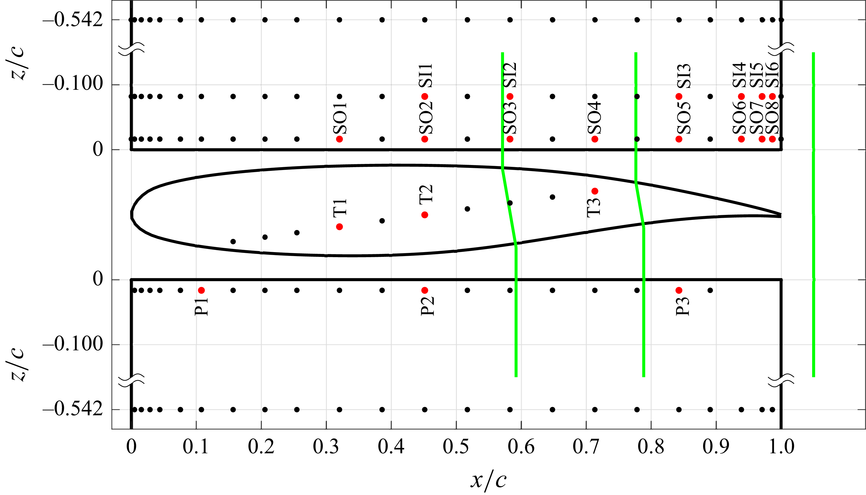


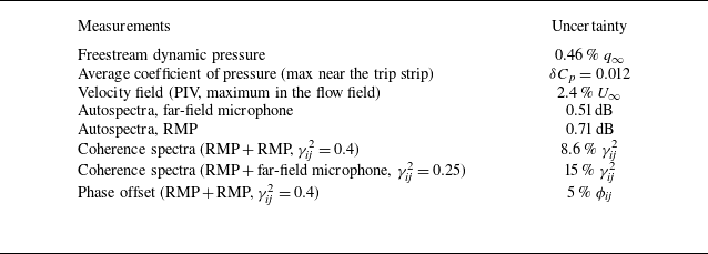


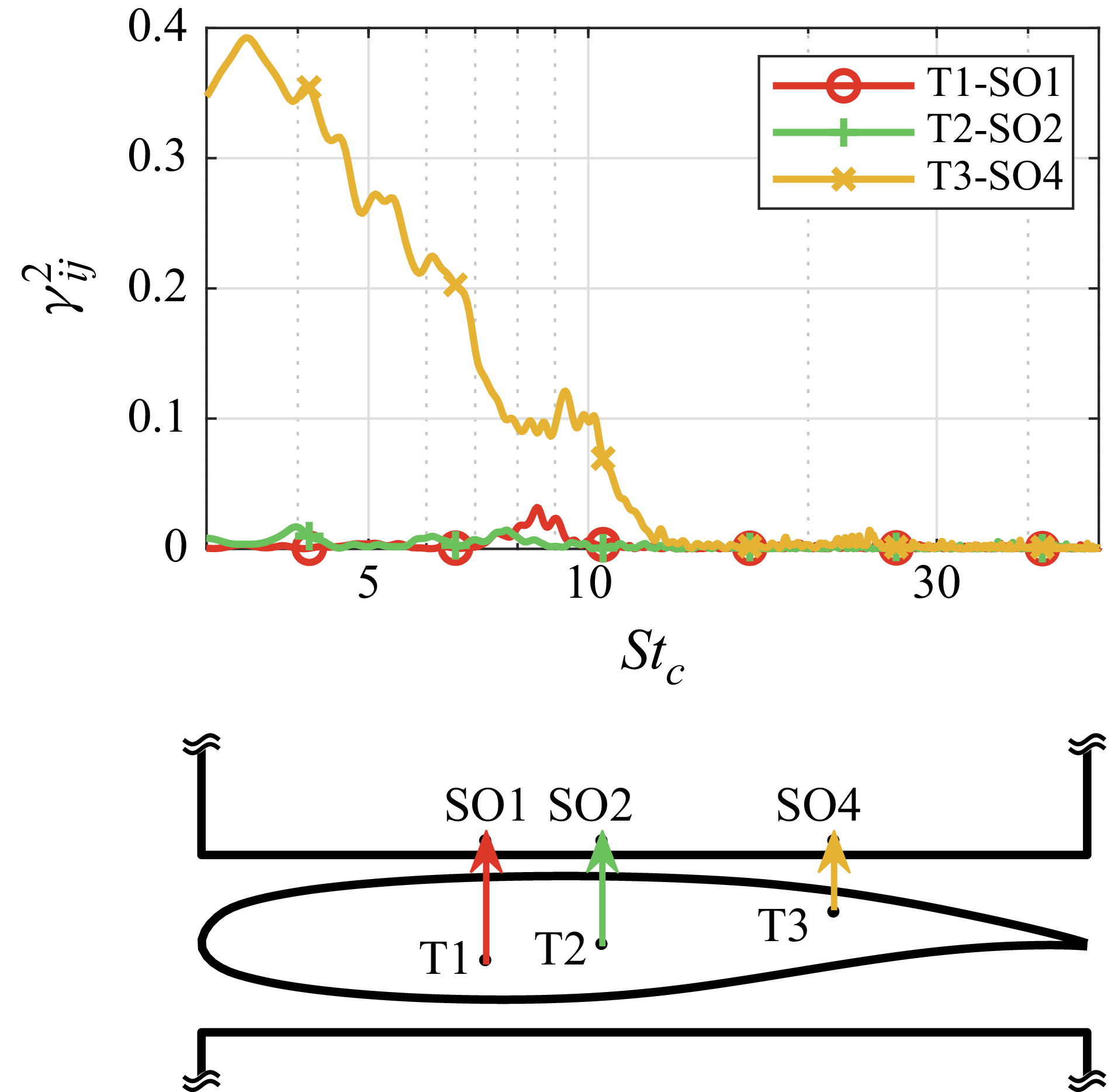
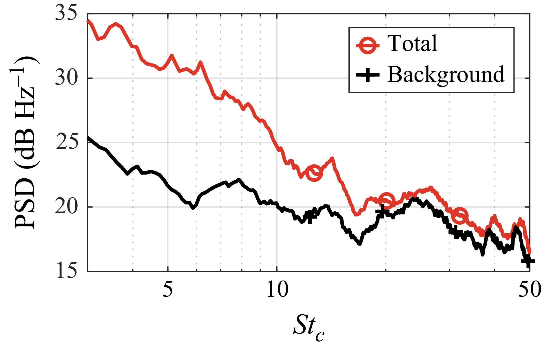


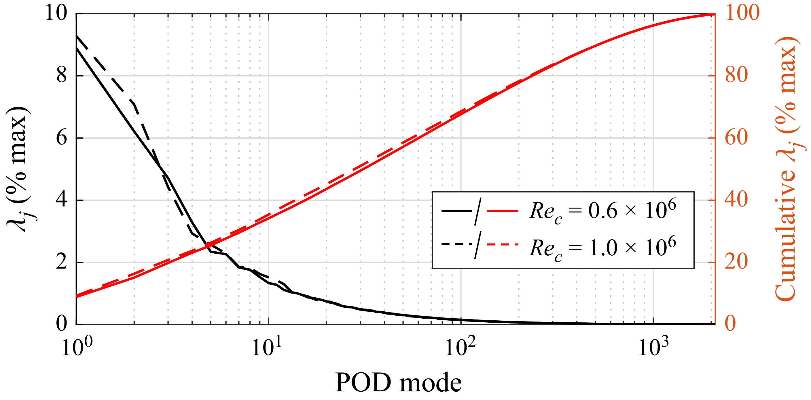


 Open access