1. Introduction
Often, the mean free path for a binary Coulomb interaction between two charged particles in the plasma that makes up the vast majority of the luminous universe is not small compared to the dynamical scales of the astrophysical system. The infrequency of collisions in these astrophysical systems necessitates a kinetic description. Kinetic equations are thus of critical importance to our understanding of astrophysical phenomena. However, the numerical integration of kinetic equations presents a significant challenge, because we require a representation of the solution in a six-dimensional phase space, three position and three velocity variables, as well as in time.
It is unequivocally true that the most common numerical techniques for the solution of kinetic equations are Monte Carlo methods. For the plasma kinetic equation, or Vlasov equation, this approach discretizes the particle distribution function as ‘macroparticles’, particles with some shape function. These macroparticles are then advanced along their characteristics and sampled to construct the required velocity moments to couple the plasma dynamics to the electromagnetic fields via Maxwell's equations (Dawson Reference Dawson1962; Langdon & Birdsall Reference Langdon and Birdsall1970; Dawson Reference Dawson1983; Birdsall & Langdon Reference Birdsall and Langdon1990; Lapenta Reference Lapenta2012). This numerical method is traditionally called the particle-in-cell (PIC) method, since the results of the velocity moment computations are deposited onto the grid that discretizes Maxwell's equations.
The PIC method has been historically very fruitful and the core method of several production-level computational tools for simulating kinetic plasmas (e.g. Fonseca et al. Reference Fonseca, Martins, Silva, Tonge, Tsung and Mori2008; Bowers et al. Reference Bowers, Albright, Yin, Daughton, Roytershteyn, Bergen and Kwan2009; Germaschewski et al. Reference Germaschewski, Fox, Abbott, Ahmadi, Maynard, Wang, Ruhl and Bhattacharjee2016). However, because of its Monte Carlo nature, the PIC method introduces counting noise into the solution of the kinetic equation. This numerical noise can manifest as a combination of numerical collisions and heating of the underlying distribution of particles and has been quantified in a number of studies (Hockney Reference Hockney1968; Okuda & Birdsall Reference Okuda and Birdsall1970; Hockney Reference Hockney1971; Okuda Reference Okuda1972; Langdon Reference Langdon1979; Krommes Reference Krommes2007).
While numerical heating can be quantified and controlled, the pollution of the solution with noise can have larger effects on the dynamics of the plasma. For example, Camporeale et al. (Reference Camporeale, Delzanno, Bergen and Moulton2016) have demonstrated that a large number of particles per cell is required to correctly identify wave–particle resonances and compare well with the wave damping rates obtained from linear theory. More egregious examples include the counting noise induced transport found to be the source of disagreement between PIC models of turbulent transport in nuclear-fusion relevant simulations and corresponding continuum models of the same flavour of turbulence (Nevins et al. Reference Nevins, Hammett, Dimits, Dorland and Shumaker2005). Here, a continuum model refers to a numerical model of a kinetic equation which directly discretizes the quantity of interest, the particle distribution function, on a phase space grid, directly solving a six-dimensional partial differential equation in time.
There are many means of reducing this noise. The simplest strategy is to use more particles, but the counting noise decreases like  $1/\sqrt {N_{\textrm {ppc}}}$, where $N_{\textrm {ppc}}$ is the number of particles per grid cell, and this slow convergence with increasing particle count can make the desired phase space accuracy prohibitively expensive computationally. Other techniques explicitly modify the algorithm, such as the delta-f PIC method (Parker & Lee Reference Parker and Lee1993; Hu & Krommes Reference Hu and Krommes1994; Denton & Kotschenreuther Reference Denton and Kotschenreuther1995; Belova, Denton & Chan Reference Belova, Denton and Chan1997; Cheng et al. Reference Cheng, Parker, Chen and Uzdensky2013; Kunz, Stone & Bai Reference Kunz, Stone and Bai2014), very high order and more sophisticated particle shape functions, e.g. particle in wavelets (van yen Nguyen et al. Reference van yen Nguyen, del Castillo-Negrete, Schneider, Farge and Chen2010, Reference van yen Nguyen, Sonnendrücker, Schneider and Farge2011) and von Mises distributions based on Kernel density estimation theory (Wu & Qin Reference Wu and Qin2018) and time-dependent deformable shape functions for the particles (Coppa et al. Reference Coppa, Lapenta, Dellapiana, Donato and Riccardo1996), the latter of which is an active area of research for the N-body Monte Carlo method applied to gravitational systems (Abel, Hahn & Kaehler Reference Abel, Hahn and Kaehler2012; Hahn & Angulo Reference Hahn and Angulo2015) and has recently been extended to PIC (Julian et al. Reference Julian, Samuel, Jonathan and Tom2016).
However, many of these modifications have their own deficiencies. The delta-f PIC method can break down if the distribution function deviates significantly from its initial value, and the modifications to the particle shape introduce significant computational complexity to the algorithm. This additional computational complexity makes application of these techniques to general kinetic systems more challenging, and preliminary work is focused on lower-dimensional systems (van yen Nguyen et al. Reference van yen Nguyen, Sonnendrücker, Schneider and Farge2011) and post-processing analysis (Totorica, Fiuza & Abel Reference Totorica, Fiuza and Abel2018). While the application of advanced particle shapes to even just the analysis of simulations pays dividends in reducing the noise in the solution (Totorica et al. Reference Totorica, Fiuza and Abel2018), any issues due to noise that arise during the course of a simulation are not mitigated.
In this paper, we document an instance of disagreement in the underlying dynamics of competing plasma instabilities when studied with a PIC simulation and continuum kinetic simulation, and trace the origin of the disagreement to the counting noise introduced to the solution by the PIC algorithm. We emphasize that the disagreement stemming from particle noise manifests not simply as numerical heating, but as a fundamental difference in the final state of the plasma's nonlinear evolution. The noise inherent to the PIC method leads to a sampling error in the computation of the current density, particularly for small numbers of particles per cell, and thus artificially introduces saturated small-scale magnetic field structure, while continuum simulations find that the magnetic field is strongly damped. Particle noise is confirmed as the result of this disagreement with a combination of larger particle count simulations and post-process filtering of the saturated state.
We are inspired by the recently reported disagreement between the continuum kinetic simulations performed in Skoutnev et al. (Reference Skoutnev, Hakim, Juno and TenBarge2019) and past PIC calculations in a similar parameter regime (Kato & Takabe Reference Kato and Takabe2008) of the competition of a class of Weibel-type instabilities driven by counter-streaming beams of plasmas (Weibel Reference Weibel1959; Bornatici & Lee Reference Bornatici and Lee1970; Davidson et al. Reference Davidson, Hammer, Haber and Wagner1972). These Weibel-type instabilities are an interesting class of plasma instabilities, serving as a possible explanation for the observed magnetic fields in gamma ray bursts (Medvedev & Loeb Reference Medvedev and Loeb1999) and pulsar wind outflows (Kazimura etal. Reference Kazimura, Sakai, Neubert and Bulanov1998), and as a potential source of the seed magnetic field in a cosmological context (Schlickeiser & Shukla Reference Schlickeiser and Shukla2003; Lazar et al. Reference Lazar, Schlickeiser, Wielebinski and Poedts2009). Importantly, while these Weibel-type instabilities robustly grow a magnetic field in the relativistic context, Skoutnev et al. (Reference Skoutnev, Hakim, Juno and TenBarge2019) found that the non-relativistic limit of these instabilities was more complex, with a spectrum of unstable modes all having comparable growth rates vying for dominance. While these Weibel-type instabilities are generally driven by counter-streaming beams of both protons and electrons, in this paper we will focus on the electron-driven variants of these instabilities.
In this regard, for the electron-driven, equal beam density and equal beam temperature, variants of these instabilities, two ratios primarily affect which mode grows the fastest:  $u_d/c$, how non-relativistic the drift velocity of the beams is, and $v_{th_e}/u_d$, how much of the initial beam energy is internal energy versus kinetic energy. Here, $u_d$ is the drift speed of each beam of electrons, $c$ is the speed of light and $v_{th_e} = \sqrt {k_B T_e/m_e}$ is the electron thermal velocity, where k B is Boltzmann's constant, T e is the electron temperature, and m e is the electron mass. In the relativistic case, $u_d \approx c$, the filamentation instability (Fried Reference Fried1959) is the fastest-growing mode and previous studies find robust magnetic field growth and saturation (Fonseca et al. Reference Fonseca, Silva, Tonge, Mori and Dawson2003; Nishikawa et al. Reference Nishikawa, Hardee, Richardson, Preece, Sol and Fishman2003, Reference Nishikawa, Hardee, Richardson, Preece, Sol and Fishman2005; Silva et al. Reference Silva, Fonseca, Tonge, Dawson, Mori and Medvedev2003; Kumar, Eichler & Gedalin Reference Kumar, Eichler and Gedalin2015; Takamoto, Matsumoto & Kato Reference Takamoto, Matsumoto and Kato2018). Likewise, as the drift velocity becomes non-relativistic, so long as the beams are ‘hot’, i.e. $v_{th_e} \approx u_d$, the disruption of the fast-growing two-stream instability leads to a secondary Weibel instability. The disruption of the saturated two-stream modes by the more slowly growing filamentation instability leads to energy conversion dominantly in only one velocity dimension, since the two-stream instability is one-dimensional, and this temperature anisotropy provides another source of free energy for the Weibel instability and thus a means of supporting a saturated magnetic field (Schlickeiser & Shukla Reference Schlickeiser and Shukla2003; Kato & Takabe Reference Kato and Takabe2008). The saturated magnetic field from the disruption of two-stream modes leads to the same levels of magnetization as previous studies of the Weibel instability and filamentation instability in isolation, in either one dimension or two dimensions (Morse & Nielson Reference Morse and Nielson1971; Califano, Pegoraro & Bulanov Reference Califano, Pegoraro and Bulanov1997; Califano et al. Reference Califano, Prandi, Pegoraro and Bulanov1998; Cagas et al. Reference Cagas, Hakim, Scales and Srinivasan2017).
These results stand in stark contrast to the findings of Skoutnev et al. (Reference Skoutnev, Hakim, Juno and TenBarge2019) as the ratio of  $v_{th_e}/u_d$ is decreased further and the inter-penetrating beams are made ‘colder’. As the temperature of the beams is reduced, the growth rates of a spectrum of oblique modes increase, modes which arise due to perturbations between parallel (two-stream) and perpendicular (filamentation) to the drift direction (Bret Reference Bret2009). These hybrid two-stream–filamentation modes begin to have comparable growth rates to the two-stream instability – see figure 1 in Skoutnev et al. (Reference Skoutnev, Hakim, Juno and TenBarge2019). These fast-growing oblique modes rapidly deplete the free energy in the inter-penetrating flows, eliminating the channel for magnetic field growth via a combination of the more slowly growing filamentation instability and secular Weibel instability from the residual temperature anisotropy of saturated two-stream modes studied in, e.g. Kato & Takabe (Reference Kato and Takabe2008).
With the free energy depleted, the oblique modes are then able to collisionlessly damp on the electrons. This collisionless damping converts the electromagnetic energy from the saturated oblique modes to electron thermal energy, leaving little residual magnetic energy in the system, along with a highly structured distribution function in phase space due to the mixing of nonlinearly saturated oblique modes. This additional phase space structure serves as an added marker for the collapse of the magnetic field via damping of the oblique modes.
The collapse of the magnetic field in the non-relativistic, cold limit in the continuum kinetic simulations presented in Skoutnev et al. (Reference Skoutnev, Hakim, Juno and TenBarge2019) had not been previously reported, and in fact disagreed with the PIC results of Kato & Takabe (Reference Kato and Takabe2008) in the ‘cold’ parameter regime,  $u_d/c = 0.1$, $v_{th_e}/u_d = 0.1$. Skoutnev et al. (Reference Skoutnev, Hakim, Juno and TenBarge2019) identified a number of potential explanations for this disagreement, such as the shock geometry – Kato & Takabe (Reference Kato and Takabe2008) performed Weibel-mediated collisionless shock simulations while Skoutnev et al. (Reference Skoutnev, Hakim, Juno and TenBarge2019) considered only perturbations to an initially unstable system and not a driven system such as a collisionless shock. In addition, Skoutnev et al. (Reference Skoutnev, Hakim, Juno and TenBarge2019) focused solely on the electron dynamics with the protons forming a neutralizing background while Kato & Takabe (Reference Kato and Takabe2008) included the dynamics of the protons in their collisionless shock simulations. We consider the effect of the difference in numerical method in this paper and perform identical simulations to Skoutnev et al. (Reference Skoutnev, Hakim, Juno and TenBarge2019) with a PIC method, focusing on the electron-only variants of these Weibel-type instabilities with an initial-value problem.
2. Methods and results
We concern ourselves with the evolution of the Vlasov equation of a species  $s$,
$s$,
 \begin{equation} \frac{\partial f_s}{\partial t} + \boldsymbol{v} \boldsymbol{\cdot} \boldsymbol{\nabla} f_s + \frac{q_s}{m_s}\left( \boldsymbol{E} + \boldsymbol{v} \times \boldsymbol{B} \right) \boldsymbol{\cdot} \boldsymbol{\nabla}_{\boldsymbol{v}} \,f_s = 0, \end{equation}
coupled to Maxwell's equations via self-consistent currents. Here, f s is the particle distribution for species s, q s and m s are the charge and mass of species $s$ respectively, and E and B are the electric and magnetic fields respectively. The Vlasov–Maxwell system of equations is numerically integrated with the PIC code p3d (Zeiler et al. Reference Zeiler, Biskamp, Drake, Rogers, Shay and Scholer2002) and the Gkeyll simulation framework, which contains a continuum Vlasov–Maxwell solver (Juno et al. Reference Juno, Hakim, TenBarge, Shi and Dorland2018). Note that the Gkeyll simulation framework also contains a Fokker–Planck collision operator, and can thus numerically integrate the Vlasov–Maxwell–Fokker–Planck system of equations (Hakim et al. Reference Hakim, Francisquez, Juno and Hammett2019).
We initialize an electron–proton plasma in two spatial dimensions and two velocity dimensions (2X2V), with two, uniform, equal density, counter-streaming, Maxwellian beams of electrons,
 \begin{equation} f_{0,e}(v_x,v_y)=\frac{n_0}{2{\rm \pi} v_{th_e}^2}\,\textrm{e}^{-{v_x^2}/{2v_{th_e}^2}}[\textrm{e}^{-{(v_y-u_d)^2}/{2v_{th_e}^2}}+\textrm{e}^{-{(v_y+u_d)^2}/{2v_{th_e}^2}}]. \end{equation}
The protons form a stationary, neutralizing background. Here,  $n_0 = 1$ is a density normalization. To excite the zoo of instabilities, two stream, filamentation (Fried Reference Fried1959) and electromagnetic oblique (Bret Reference Bret2009), a collection of electric and magnetic fluctuations are initialized,
 \begin{equation} B_z(t=0) = \sum_{n_x, n_y = 0}^{16, 16} \tilde{B} \sin\left( \frac{2 {\rm \pi}n_x x}{L_x} + \frac{2 {\rm \pi}n_y y}{L_y} + \tilde{\phi}\right ), \end{equation}
with equivalent perturbations in  $E_x$ and $E_y$. Here, $\tilde {B}$ and $\tilde {\phi }$ are random amplitudes and phases, with the random amplitudes chosen such that all three fields have equal initial average energy densities, $\langle \epsilon _0 E_x^2/2 \rangle = \langle \epsilon _0 E_y^2/2 \rangle = \langle B_z^2/2\mu _0 \rangle \approx 10^{-7} E_K$, where $E_K$ is the total initial energy of the two counter-streaming beams of electrons and $\epsilon_0$ and $\mu_0$ are the permittivity and permeability of free space respectively.
Further details of the simulations are as follows. For all simulations, the box size is chosen based on the  $u_d/c = 0.1$, $v_{th_e}/u_d = 0.1$ simulation in Skoutnev et al. (Reference Skoutnev, Hakim, Juno and TenBarge2019), $L_x = 2.7 d_e$, $L_y = 3.1 d_e$, where $d_e = c/\omega _{\textrm {pe}}$ is the electron inertial length and $\omega _{\textrm {pe}} = \sqrt {e^2 n_e/\epsilon _0 m_e}$ is the electron plasma frequency. This box size is chosen to fit the faster-growing filamentation mode, $k_{\textrm {max}}^{\textrm {FI}} = 2 {\rm \pi}/L_x$, and an integer number of two-stream modes $k_{\textrm {max}}^{\textrm {TS}} = 2 {\rm \pi}n/L_y$, while keeping the box size roughly square $L_x \approx L_y$. The Gkeyll continuum Vlasov–Maxwell simulation is run with $N_x = N_y = 48$ grid points in configuration space, $v_{\textrm {max}} = [-3 u_d, 3 u_d]$ velocity space extents, $N_v = 64^2$ in the two velocity dimensions and piecewise quadratic Serendipity elements (Arnold & Awanou Reference Arnold and Awanou2011) – see Juno et al. (Reference Juno, Hakim, TenBarge, Shi and Dorland2018) for details on the discontinuous Galerkin discretization of the Vlasov–Maxwell system of equations. The p3d simulations are run with configuration space resolution ${\rm \Delta} x = {\rm \Delta} y = 0.014 d_e$, and the number of particles per cell is varied according to $N_{\textrm {ppc}} = [12, 120, 1200, 12\,000]$, with both linear and quadratic particle shapes. In addition, the p3d simulations employ Marder's correction (Marder Reference Marder1987) via a multigrid method to enforce charge conservation. Periodic boundary conditions are employed in configuration space, and for only the continuum Gkeyll simulation, zero-flux boundary conditions are used in velocity space, along with a small number of collisions, $\nu _{ee} = 4 \times 10^{-5} \omega _{\textrm {pe}}$, for velocity space regularization – see Hakim et al. (Reference Hakim, Francisquez, Juno and Hammett2019) for details of the collision operator implementation in Gkeyll.
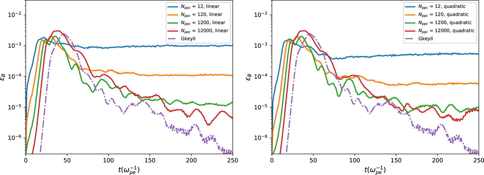
The evolution of the box-integrated magnetic energy from this suite of simulations is shown in figure 1. We can clearly identify the collapse of the magnetic field observed in Skoutnev et al. (Reference Skoutnev, Hakim, Juno and TenBarge2019) in both the continuum Gkeyll simulations and the high particle count p3d simulations. However, as the number of particles per cell is decreased, the magnetic field attains a particle-per-cell-dependent saturated state. The saturation level has some sensitivity to the particle shape, with the quadratic spline particles saturating at a lower level than the linear spline particles. But even the modestly high particle counts saturate at a still higher amplitude than what we expect from the continuum calculation and more resolved PIC calculations.
Evolution of the box-integrated magnetic field energy,  $\epsilon _B = 1/(2 \mu _0) \int B_z^2$, normalized to the initial electron energy for a sequence of p3d calculations varying particle number and particle shape and compared to a fiducial Gkeyll calculation. While there is initial growth of the magnetic field due to the electromagnetic component of the oblique modes, the oblique modes quickly damp the electrons, leading to the decay of the magnetic field energy in the continuum Gkeyll simulation and high particle count p3d simulations. With the free energy of the counter-streaming electron beams depleted by the fast-growing oblique modes, the continuum and more highly resolved PIC calculations cannot support any saturated magnetic field structure. However, with reduced particle count, the magnetic field energy saturates to a fixed value. Modest increases in the number of particles per cell and higher-order particle shapes reduce the magnitude of the saturated magnetic field, but only with more substantial increases in particle count do we observe similar late time behaviour between the p3d PIC and Gkeyll continuum simulations.

To understand this pseudo-saturation of the magnetic field, we show the phase space structure from the Gkeyll simulation and a subset of the p3d simulations in figures 2 and3. We plot the results from the Gkeyll simulation (left column), along with the  $N_{\textrm {ppc}} = 12$ and $N_{\textrm {ppc}} = 12\,000$, quadratic spline particle shape, p3d simulations (middle and right columns) in $y-v_y$ (figure 2) and $v_x-v_y$ (figure 3). The three rows denote the beginning of the simulation, $t = 0 \omega _{\textrm {pe}}^{-1}$ (top row), peak of the magnetic field energy, $t = 45 \omega _{\textrm {pe}}^{-1}$ for the Gkeyll simulation and $t = 35 \omega _{\textrm {pe}}^{-1}$ for the p3d simulations (middle row) and end of the simulation, $t = 250 \omega _{\textrm {pe}}^{-1}$ (bottom row). These distribution function cuts are generated from the full 2X2V phase space by integrating over the interior $0.1 d_e$ in the $x$ dimension, i.e. the middle two grid cells in $x$ in the Gkeyll simulation, and the equivalent $x$ extents in the p3d simulations, along with an integration in the entirety of $v_x$ for the $y-v_y$ cut in figure 2, and the entirety of $y$ for the $v_x-v_y$ cut in figure 3. We note that to generate the velocity space representation in the p3d simulations, the particles are binned into 101 equally spaced bins from $-20 v_{th_e}$ to $20 v_{th_e}$ in $v_y$ for figure 2 and both $v_x$ and $v_y$ for figure 3.
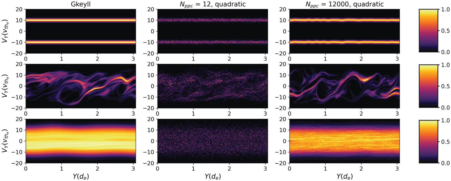
Evolution of the electron distribution function from Gkeyll (left column) and  $N_{\textrm {ppc}}=12$ and $N_{\textrm {ppc}} = 12\,000$, quadratic spline, p3d (middle and right column) simulations in $y-v_y$. The rows show the evolution of the distribution function in time, $t = 0 \omega _{\textrm {pe}}^{-1}$ (top row), the peak of the magnetic field energy, $t = 45 \omega _{\textrm {pe}}^{-1}$ for the Gkeyll simulation and $t = 35 \omega _{\textrm {pe}}^{-1}$ for the p3d simulations (middle row) and the end of the simulation $t = 250 \omega _{\textrm {pe}}^{-1}$ (bottom row). These distribution function cuts are generated by integrating over a narrow slice of the interior of $L_x$ and all of $v_x$. Specifically, we integrate the Gkeyll simulation over the middle two grid cells, ${\rm \Delta} x = 0.1 d_e$, and sample particles from the corresponding extent in the p3d simulations. In addition, to generate the velocity space representation in $v_y$ of the p3d simulations, the particles are binned into 101 equally space bins from $-20 v_{th_e}$ to $20 v_{th_e}$. All three simulations begin with good phase space resolution, as the initial particle distribution function can be sampled precisely even with only $N_{\textrm {ppc}} = 12$. However, we can see that the evolution of phase space is much less well resolved with very few particles per cell, and because the nonlinear dynamics of the saturated instabilities leads to a phase space filling electron distribution function, the effective phase space resolution of the $N_{\textrm {ppc}} = 12$ calculation has decreased significantly by the end of the simulation.

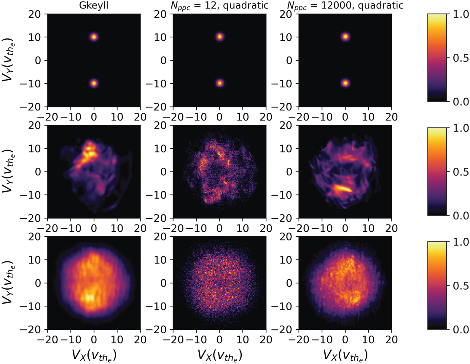
The same evolution of the electron distribution function shown in figure 2 from Gkeyll (left column) and  $N_{\textrm {ppc}}=12$ and $N_{\textrm {ppc}} = 12\,000$, quadratic spline, p3d (middle and right column) simulations, but now in $v_x-v_y$. The rows show the evolution of the distribution function in time, $t = 0 \omega _{\textrm {pe}}^{-1}$ (top row), the peak of the magnetic field energy, $t = 45 \omega _{\textrm {pe}}^{-1}$ for the Gkeyll simulation and $t = 35 \omega _{\textrm {pe}}^{-1}$ for the p3d simulations (middle row) and the end of the simulation $t = 250 \omega _{\textrm {pe}}^{-1}$ (bottom row). These distribution function cuts are generated by integrating over a narrow slice of the interior of $L_x$ and all of $y$. As in figure 2, we integrate the Gkeyll simulation over the middle two grid cells, ${\rm \Delta} x = 0.1 d_e$, and sample particles from the corresponding extent in the p3d simulations. In addition, to generate the velocity space representation in $v_x$ and $v_y$ of the p3d simulations, the particles are binned into 101 equally space bins from $-20 v_{th_e}$ to $20 v_{th_e}$ for both velocity dimensions. Again, the phase space resolution at the beginning of the simulation is acceptable, even with only $N_{\textrm {ppc}} = 12$, because we can sample particles efficiently for the cold distribution. However, because the unstable oblique modes efficiently convert this free energy into electromagnetic energy and then back into electron thermal energy, the final electron distribution fills a much larger volume of phase space and the effective phase space resolution has plummeted by the end of the simulation.

We observe that, regardless of the ‘coarseness’ of our particle resolution, the simulations begin with good phase space resolution. Although the beams are cold and the drift speed is large,  $u_d \gg v_{th_e}$, even with $N_{\textrm {ppc}} = 12$, we can concentrate phase space resolution in the initial distribution function for the p3d calculations. However, as the instabilities evolve and lead to the electrons filling phase space, the low particle count simulation in figures 2 and 3 becomes much less well resolved, with an inability to distinguish the features observed at saturation in the Gkeyll and $N_{\textrm {ppc}} = 12\,000$ simulations, and the steady-state isotropic distribution becoming poorly sampled.
To understand the effect this decreased effective phase space resolution can have on the dynamics of the plasma in the  $N_{\textrm {ppc}} = 12$ p3d simulation, consider Ampère's law in steady state,
 \begin{equation} \boldsymbol{\nabla}_{\boldsymbol{x}} \times \boldsymbol{B} = \mu_0 \boldsymbol{J} = \mu_0 \sum_s q_s \int \boldsymbol{v} f_s \,\textrm{d}\boldsymbol{v}, \end{equation}
where we have assumed  $\partial \boldsymbol {E}/\partial t \rightarrow 0$ and substituted the charge-weighted sum over each species’ first velocity moment for the current density. While this computation of the current is straightforward for the grid-based continuum method in Gkeyll, for the p3d PIC calculations this velocity moment is given by the sum over each individual macroparticle's velocity
 \begin{equation} \sum_s q_s \int \boldsymbol{v} f_s \, \textrm{d}\boldsymbol{v} = \sum_s q^{\textrm{PIC}}_s \sum_{j=1}^N \boldsymbol{V}_{s,j} S (\boldsymbol{x} - \boldsymbol{X}_{s,j}), \end{equation}
where  $\boldsymbol {X}_{s,j}$ and $\boldsymbol {V}_{s,j}$ are the $j$ macroparticle positions and velocities for species $s$,
$s$,  $q^{\textrm {PIC}}_s$ is the charge of the macroparticle of species $s$ and $S(\boldsymbol {x})$ is the shape function in configuration space.
Because the current density is computed from discrete macroparticles, if any fluctuations in the current density are uncorrelated on some spatial scale, we expect these fluctuations can give rise to a magnetic field. This behaviour would be akin to the ‘quasi-thermal’, electrostatic noise which arises from uncorrelated density fluctuations in a plasma, both in real plasma systems (Meyer-Vernet et al. Reference Meyer-Vernet, Couturier, Hoang, Perche, Steinberg, Fainberg and Meetre1986) and in PIC calculations (Langdon Reference Langdon1979). We expect, in analogy with the Debye length for electrostatic shielding and density fluctuations, the electron skin depth,  $d_e$, is the scale below which current density fluctuations will not be effectively shielded by the magnetic field. Since these fluctuations are uncorrelated, their ensemble average, i.e. their average over many realizations of the plasma system, will be zero, but their root-mean-square (r.m.s.) average might not be zero. In other words, the current density computed from the collection has zero ensemble average,
 \begin{equation} \left \langle \boldsymbol{J}^{\textrm{PIC}} \right \rangle = \sum_s q^{\textrm{PIC}}_s \left \langle \sum_j \boldsymbol{V}_{s,j} S (\boldsymbol{x} - \boldsymbol{X}_{s,j}) \right \rangle = 0, \end{equation}
where  $\langle \cdot \rangle$ denotes the ensemble average, but the squared r.m.s.,
 \begin{equation} \left |\boldsymbol{J}_{\textrm{ rms}}^{\textrm{PIC}} \right |^2 = \sum_s \frac{1}{N^{\textrm{PIC}}}\left (q^{\textrm{PIC}}_s \right)^2 \sum_j \sum_k \boldsymbol{V}_{s,j} S (\boldsymbol{x} - \boldsymbol{X}_{s,j}) \boldsymbol{V}_{s,k} S (\boldsymbol{x} - \boldsymbol{X}_{s,k}), \end{equation}
where  $N^{\textrm {PIC}}$ is the number of PIC particles being summed over, may have non-zero ensemble average,
 \begin{equation} \left \langle \left | \boldsymbol{J}_{\textrm{ rms}}^{\textrm{PIC}} \right |^2 \right \rangle = \sum_s \frac{1}{N^{\textrm{PIC}}} \left ( q^{\textrm{PIC}}_s \right)^2 \left \langle \sum_j \sum_k \boldsymbol{V}_{s,j} S (\boldsymbol{x} - \boldsymbol{X}_{s,j}) \boldsymbol{V}_{s,k} S (\boldsymbol{x} - \boldsymbol{X}_{s,k}) \right \rangle \neq 0. \end{equation}
 If we assume the current is carried solely by the electrons and consider a volume of  $\sim d_e^2$ in two dimensions, we can make a back-of-the-envelope calculation for the size of the r.m.s. current density,
 \begin{align} \left \langle \left | \boldsymbol{J}_{\textrm{ rms}}^{\textrm{PIC}} \right |^2 \right \rangle & \sim \frac{ \left (e^{\textrm{PIC}} \right )^2}{ \left ( d_e^{\textrm{PIC}} \right )^4} \frac{1}{N^{\textrm{PIC}}} \sum_j \left \langle |\boldsymbol{V}_j|^2 \right \rangle \nonumber\\ & \sim \frac{ \left (e^{\textrm{PIC}} \right )^2}{ \left ( d_e^{\textrm{PIC}} \right )^4} N^{\textrm{PIC}} \left (v^{\textrm{PIC}}_{th_e} \right )^2, \end{align}
where we have added the superscript  $PIC$ to all quantities, charge, $e^{\textrm {PIC}}$, electron inertial length, $d_e^{\textrm {PIC}}$ and electron thermal velocity $v_{th_e}^{\textrm {PIC}}$ to emphasize these are the macroparticle quantities.
In general, because a macroparticle represents many particles in the real plasma system, all intrinsic properties, e.g. the mass and charge, must be scaled by the appropriate macroparticle factor when comparing a quantity computed with the PIC method to the actual physical quantity. Comparing the r.m.s. current density from the PIC method to the physical r.m.s. current density from a fiducial plasma, we have
 \begin{equation} \frac{\left \langle \left | \boldsymbol{J}_{\textrm{rms}}^{\textrm{PIC}} \right |^2 \right \rangle}{\left \langle \left | \boldsymbol{J}_{\textrm{rms}} \right |^2 \right \rangle} = \frac{\dfrac{\left (e^{\textrm{PIC}} \right )^2}{\left ( d_e^{\textrm{PIC}} \right )^4} N^{\textrm{PIC}} \left (v^{\textrm{PIC}}_{th_e} \right )^2}{\dfrac{e^2}{d_e^4} N v_{th_e}^2}, \end{equation}
where  $N$ is the number of particles in the real plasma system being modelled. Since every charge is a macroparticle charge, the difference between the macroparticle charge and the elementary charge is
 \begin{equation} \frac{e^{\textrm{PIC}}}{e} = \frac{F^{\textrm{macro}} e}{e} = \frac{N}{N_{\textrm{ppc}} N_{\textrm{cells}}}, \end{equation}
where  $F^{\textrm {macro}}$ is the scaling factor for the number of particles a macroparticle represents and $N_{\textrm {cells}}$ is the number of grid cells we have summed over to construct our $d_e^2$ volume. In other words, when $N_{\textrm {ppc}} N_{\textrm {cells}} < N$, the charge in the PIC method must be scaled by the appropriate factor since the macroparticle is representing some (potentially large) number of particles.
We can proceed in a similar fashion for the other terms. We note that the electron plasma frequency,  $\omega _{\textrm {pe}} = \sqrt {e^2 n/\epsilon _0 m_e}$, is macroparticle independent because the macroparticle factors cancel in the charge, density and mass. Therefore, the electron inertial length, $d_e = c/\omega _{\textrm {pe}}$, is also macroparticle independent. To determine the factor for the electron thermal velocity, we note that substitution of one factor of $d_e^2$ reveals that
 \begin{equation} \frac{\left (v_{th_e}^{\textrm{PIC}} \right )^2}{d_e^2} = \frac{\left (v_{th_e}^{\textrm{PIC}} \right )^2}{c^2} \omega_{\textrm{pe}}^2, \end{equation}
and since the ratio of the electron thermal velocity to the speed of light is independent of macroparticle size, we have no additional factor from the electron thermal velocity. We are thus left with
 \begin{equation} \frac{\left \langle \left |\boldsymbol{J}_{\textrm{rms}}^{\textrm{PIC}} \right |^2 \right \rangle}{\left \langle \left | \boldsymbol{J}_{\textrm{rms}} \right |^2 \right \rangle} = \frac{N}{N_{\textrm{ppc}} N_{\textrm{cells}}}, \end{equation}
after substitution of  $N^{\textrm {PIC}} = N_{\textrm {ppc}} N_{\textrm {cells}}$. We can then massage (2.9) to a more general form with the appropriate scaling factor,
 \begin{equation} \left \langle \left |\boldsymbol{J}_{\textrm{ rms}}^{\textrm{PIC}} \right |^2 \right \rangle \sim \left (\frac{N}{N_{\textrm{cells}} N_{\textrm{ppc}}} \right ) \frac{e^2}{d_e^2} n v^2_{th_e}, \end{equation}
where  $n$ is the number density of the plasma. In the limit that every macroparticle represents a single charged particle in the real plasma system, (2.14) would reduce to the estimate of the continuum r.m.s. current density spectrum from uncorrelated current density fluctuations.
Substitution of the estimate in (2.14) into Ampère's law gives us
 \begin{align} \frac{1}{2\mu_0} \left \langle \left |\boldsymbol{B}_{\textrm{ rms}}^{\textrm{PIC}} \right |^2 \right \rangle & \sim \frac{d^2_e \mu_0}{2} \left \langle \left | \boldsymbol{J}_{\textrm{rms}}^{\textrm{PIC}} \right |^2 \right \rangle \nonumber\\ & \sim \left (\frac{N}{N_{\textrm{cells}} N_{\textrm{ppc}}} \right ) \frac{d^2_e \mu_0}{2} \frac{e^2}{d_e^2} n v^2_{th_e}, \end{align}
which, upon rearrangement of the expression using the fact that  $c^2 = 1/\epsilon _0 \mu _0$ and our definitions of the electron thermal velocity, $v_{th_e}$, the electron plasma frequency, $\omega _{\textrm {pe}}$, and electron skin depth, $d_e$, we obtain
 \begin{align} \frac{1}{2\mu_0} \left \langle \left | \boldsymbol{B}_{\textrm{ rms}}^{\textrm{PIC}} \right |^2 \right \rangle & \sim \frac{1}{2} \frac{N}{N_{\textrm{cells}} N_{\textrm{ppc}}} \frac{T}{d_e^2}\nonumber\\ & \sim \frac{1}{2} \frac{n T}{N_{\textrm{cells}} N_{\textrm{ppc}}}. \end{align}
This estimate is similar to Tajima et al. (Reference Tajima, Cable, Shibata and Kulsrud1992) for the continuum noise spectrum of current fluctuations, but with the additional  $N_{\textrm {cells}} N_{\textrm {ppc}}$ term for how the fluctuation spectrum scales with the number of particles per cell. However, this calculation is fundamentally different from the Tajima et al. (Reference Tajima, Cable, Shibata and Kulsrud1992) computation of the continuum noise spectra because we expect the fluctuation spectrum to decrease with increasing $N_{\textrm {ppc}}$, as we are estimating an anomalous source of fluctuations. The PIC method is still a numerical discretization of the Vlasov equation, which in the absence of true discrete particle effects such as collisions should not have a fluctuation spectrum due to uncorrelated current density fluctuations.
We note that the magnitude of the magnetic field fluctuations in (2.16) inversely depends on the number of particles per cell, as we expect from the scaling of the saturated magnetic field amplitude in figure 1, where we observe the saturation level decreasing by roughly an order of magnitude when we increase the number of particles by a factor of ten. Importantly, the magnitude of the magnetic field fluctuations also depends on the temperature, thus explaining the observed saturated magnetic field state in the smaller  $N_{\textrm {ppc}}$ p3d simulations. Despite a reasonable sampling accuracy at the beginning of the simulation for the initially cold beams, the large electron temperature increase from the oblique mode dynamics leads to a larger noise floor of magnetic field fluctuations. In other words, the number of particles per cell, $N_{\textrm {ppc}}$, is fixed, so increases in the temperature of the distribution being sampled inevitably increases the fluctuation amplitude arising from noise. By the end of the simulation, we are much more poorly sampling the saturated electron distribution function because of the distribution's increased temperature, and we thus obtain a saturated magnetic field from the resulting r.m.s. fluctuations in the current density. The final, much hotter, electron distribution would require higher phase space resolution, i.e. a larger number of particles per cell, to effectively represent and reduce the r.m.s. current density fluctuations which arise from the noise inherent to the PIC method.
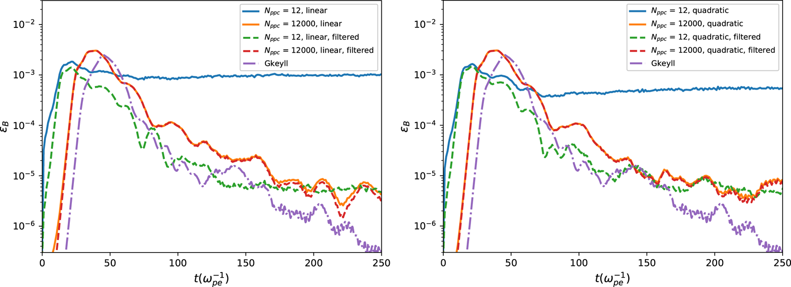
It is natural to ask if this noise-generated magnetic field can be filtered in some fashion to restore the solution to the results found in the continuum Gkeyll simulation and converged p3d simulations. We plot in figure 4 the result of a boxcar smoothing on a  $3 \times 3$ stencil in configuration space, i.e. a spatial average over the smallest scales in the p3d simulation. Clearly, the averaging over the small spatial scales assists in the restoration of the collapse of the magnetic field, even if the p3d calculations still do not reproduce the exact quantitative level of collapse as the Gkeyll simulations. We emphasize that the filtering procedure performed here is done in post-processing, and while this post-processing procedure works here for this initial-value problem, we caution that for a driven system such as a Weibel-mediated collisionless shock, in situ filtering may be required to restore the results of instability collapse, lest a pseudo-saturated magnetic field pollute the dynamics of the driven system. But, aggressive in situ filtering should also be employed with caution, as it is the saturated oblique modes that lead to the magnetic field collapse, and filtering in situ may average over the oblique mode dynamics and prevent the collisionless damping of the electromagnetic fluctuations.
Evolution of the box-integrated magnetic field energy,  $\epsilon _B = 1/(2 \mu _0) \int B_z^2$, normalized to the initial electron energy, with a $3 \times 3$ spatial boxcar filter applied in post-processing to the $N_{\textrm {ppc}} = 12$ and $N_{\textrm {ppc}} = 12\,000$ p3d simulations, with the corresponding unfiltered p3d data and the Gkeyll simulation for reference. The use of a filter on small spatial scales assists in the smoothing of the noise-generated magnetic field for this initial-value problem, although the magnitude of the magnetic field collapse still does not agree with the fiducial Gkeyll simulation.

3. Discussion and summary
We conclude having demonstrated the role particle noise can play in the dynamics of the electron-only variants of Weibel-type instabilities. In the non-relativistic, cold limit, we should find no net magnetization from the free energy of the initial counter-streaming electron beams due to the dynamically important electromagnetic oblique modes depleting this free energy and then damping the magnetic field, but a particle-per-cell-dependent saturated magnetic field can arise in underresolved PIC simulations due to noise-generated fluctuations in the current density. This result on its own suggests a re-examination of some Weibel-relevant calculations may be necessary to accurately assess the role of these electromagnetic oblique modes. The noise-driven saturated magnetic field in the low  $N_{\textrm {ppc}}$ simulations is motivating for collisionless shock simulations with the PIC method, which often employ $N_{\textrm {ppc}} = 10\text {--}100$ (see, e.g. Spitkovsky Reference Spitkovsky, Bulik, Rudak and Madejski2005; Kato & Takabe Reference Kato and Takabe2008; Fiuza et al. Reference Fiuza, Fonseca, Tonge, Mori and Silva2012; Huntington et al. Reference Huntington, Fiuza, Ross, Zylstra, Drake, Froula, Gregori, Kugland, Kuranz and Levy2015). Beyond a re-exploration of Weibel-mediated collisionless shocks in the parameter regime considered here, studies of the Biermann battery (Biermann Reference Biermann1950), another candidate for the development of a magnetic field in the very early universe, have found the presence of the electron Weibel instability as one pushes to larger system size (Schoeffler et al. Reference Schoeffler, Loureiro, Fonseca and Silva2014, Reference Schoeffler, Loureiro, Fonseca and Silva2016; Schoeffler, Loureiro & Silva Reference Schoeffler, Loureiro and Silva2018). Thus, a study of the Biermann battery in this ‘cold’ parameter regime is both timely due to the discovery of the importance of the oblique mode dynamics by Skoutnev et al. (Reference Skoutnev, Hakim, Juno and TenBarge2019) and likely requires care given the results presented here on the sensitivity of the oblique mode dynamics to phase space resolution.
We do not wish to appear antagonistic towards the PIC method. There are applications which historically have used fewer particles per cell, and our study suggests the physics of oblique modes requires higher effective phase space resolution. In general, the phase space resolution required for a kinetic simulation to adequately represent the physics of interest is difficult to know a priori (see, e.g. Barnes, Dorland & Tatsuno Reference Barnes, Dorland and Tatsuno2010). It is not necessarily surprising that certain phenomena may require higher phase space resolution. In this regard, the continuum method employed here should be viewed as a complementary approach to the general task of modelling kinetic plasmas because of the high resolution the method provides in phase space at an acceptable computational cost – the  $N_{\textrm {ppc}} = 1200$ linear spline p3d simulation has roughly the same cost as the $48^2 \times 64^2$, piecewise quadratic Serendipity element Gkeyll simulation. We believe the power of this complementary continuum kinetic approach is made manifest by the results of this study, in addition to previous studies of similar phenomena in the unmagnetized regime, such as collisionless shocks (Pusztai et al. Reference Pusztai, TenBarge, Csapó, Juno, Hakim, Yi and Fülöp2018; Sundström et al. Reference Sundström, Juno, TenBarge and Pusztai2019), the one-dimensional Weibel instability (Cagas et al. Reference Cagas, Hakim, Scales and Srinivasan2017), and the plasma dynamo (Pusztai et al. Reference Pusztai, Juno, Brandenburg, TenBarge, Hakim, Francisquez and Sundström2020).
We wish to emphasize that the results of this study alone do not yet answer the question of the source of disagreement between Skoutnev et al. (Reference Skoutnev, Hakim, Juno and TenBarge2019) and Kato & Takabe (Reference Kato and Takabe2008) in the non-relativistic, cold parameter regime. On one hand, particle noise appears to be a possible component of the disagreement, with the potential for a noise-generated magnetic field to modify the dynamics in a driven system such as a Weibel-mediated collisionless shock. On the other hand, this comparison is incomplete until the effects of the protons and shock geometry are also considered. A recent study (Matteucci et al. Reference Matteucci, Fox, Bhattacharjee, Schaeffer, Germaschewski, Fiksel, Peery and Hu2019), found that the growth of the magnetic field in laser ablation simulations matched solely the ion Weibel theory, as opposed to the combined ion–electron Weibel theory. In this non-relativistic parameter regime, it is possible that the protons, or more generally any ion species, are solely responsible or magnetic field growth, and the protons receive no assistance from the electron Weibel instability due to the oblique mode dynamics of the electrons. A further study of the phase space dynamics of the proton Weibel instability will be the focus of a future study.
Finally, we end with a note that the results of this study prompt an additional inquiry analogous to the original studies of quasi-thermal noise in PIC codes, such as the numerical fluctuation–dissipation relation derived in Langdon (Reference Langdon1979). All of the previous work in quantifying noise in the PIC method has focused on the uncorrelated charge density fluctuations and the corresponding noise-driven electrostatic field from these fluctuations. While uncorrelated charge density fluctuations lead to uncorrelated current density fluctuations via the equation of charge continuity, and violations of charge continuity are themselves a source of noise which can be mitigated via additional improvements to the particle-in-cell method such as energy-conserving methods (Markidis & Lapenta Reference Markidis and Lapenta2011), we note that the p3d simulations considered here employ Marder's correction (Marder Reference Marder1987) to the charge density to mitigate such errors. Thus, we take as motivation this observed noise-driven magnetic field to propose an extension of the previous work quantifying noise in the PIC method, rederiving the modern results for the continuum magnetic field spectra of real plasmas (Yoon Reference Yoon2007; Schlickeiser & Yoon Reference Schlickeiser and Yoon2012; Yoon, Schlickeiser & Kolberg Reference Yoon, Schlickeiser and Kolberg2014) but using particles with finite shape. In much the same way as the results of Langdon (Reference Langdon1979) permit PIC codes to carefully filter and control electrostatic noise (Haggerty et al. Reference Haggerty, Parashar, Matthaeus, Shay, Yang, Wan, Wu and Servidio2017) by providing precise predictions of the noise generated by density fluctuations of the macroparticles, a similar prediction could be calculated from a fluctuation–dissipation relation on the magnitude of magnetic field fluctuations generated by current density fluctuations of the macroparticles.
Acknowledgements
The authors wish to thank G. W. Hammett and W. Dorland for enlightening conversations on estimating particle noise, as well as the insights of the entire Gkeyll team. This work used the Extreme Science and Engineering Discovery Environment (XSEDE), which is supported by National Science Foundation grant number ACI-1548562, and resources of the National Energy Research Scientific Computing Center (NERSC), a U.S. Department of Energy Office of Science User Facility operated under Contract No. DE-AC02-05CH11231. J.J. was supported by a NASA Earth and Space Science Fellowship (Grant No. 80NSSC17K0428). M.S. was supported by NASA Grant No. 80NSSC19K039. J.M.T. was supported by NSF SHINE award AGS-1622306. V.S. was supported by Max-Planck/Princeton Center for Plasma Physics (NSF grant PHY-1804048). A.H. is supported by the High-Fidelity Boundary Plasma Simulation SciDAC Project, part of the DOE Scientific Discovery Through Advanced Computing (SciDAC) program, through the U.S. Department of Energy contract No. DE-AC02-09CH11466 for the Princeton Plasma Physics Laboratory and by Air Force Office of Scientific Research under Grant No. FA9550-15-1-0193.