2. Governing equations and numerical simulation approach

To obtain the baseflow solution, the CNSE are solved in conservative form for an ideal, Newtonian, non-reactive gas and written in vector form as a system of time evolving partial differential equations

(2.1)\begin{equation} \frac{\partial \boldsymbol{W}}{\partial t} + \frac{\partial \boldsymbol{E}}{\partial x} + \frac{\partial \boldsymbol{F}}{\partial y} + \frac{\partial \boldsymbol{G}}{\partial z} = 0, \end{equation}

where $\boldsymbol {W}=[\rho,\rho u, \rho v, \rho w, \rho E_t]^{\rm T}$ is the conservative state vector, $\rho,u, v, w$ and $E_t$ are the density, $x$, $y$ and $z$ components of the velocity and total energy, respectively. Total energy can be written in the form

(2.2)\begin{equation} E_t = \frac{R_gT}{\gamma -1} + \frac{u^2 + v^2 + w^2}{2}. \end{equation}

Here $\boldsymbol {E}$, $\boldsymbol {F}$ and $\boldsymbol {G}$ are the combined convective and viscous flux vectors that can be written as

(2.3)\begin{gather} \boldsymbol{E}= \left[ \begin{array}{@{}c@{}} \rho u \\ \rho u^2 + p -\tau_{xx} \\ \rho u v -\tau_{xy} \\ \rho u w -\tau_{xz} \\ (\rho E_t + p)u -u \tau_{xx} - v\tau_{xy} - w\tau_{xz} + q_x \end{array} \right], \end{gather}

(2.4)\begin{gather} \boldsymbol{F}= \left[ \begin{array}{@{}c@{}} \rho v \\ \rho uv -\tau_{xy} \\ \rho v^2 +p -\tau_{yy} \\ \rho vw -\tau_{yz} \\ (\rho E_t + p)v -u \tau_{xy} - v\tau_{yy} -w \tau_{yz} + q_y \end{array} \right], \end{gather}

(2.5)\begin{gather} \boldsymbol{G}= \left[ \begin{array}{@{}c@{}} \rho w \\ \rho uw -\tau_{xz} \\ \rho vw -\tau_{yz} \\ \rho w^2 + p -\tau_{zz} \\ (\rho E_t + p)w -u \tau_{xz} - v\tau_{yz} -w \tau_{zz} + q_z \end{array} \right], \end{gather}

where $\tau _{ij}$ are the stress tensor components and $q_i$ are the heat flux vector components in the $x$, $y$ and $z$ directions. The viscosity $\mu$ is calculated utilizing Sutherland's law with a low temperature correction

(2.6)\begin{equation} \mu = \begin{cases} S_1 T_1, & \text{for }T < T_1, \\ S_1 T, & \text{for }T_1 \leq T \leq T_2, \text{and} \\ \dfrac{S_2 T^{3/2}}{T+T_2}, & \text{for }T > T_2, \\ \end{cases} \end{equation}

where $S_1=6.93873\times 10^{-8}\,\text {Ns}\,(\text {m}^{2}\,\text {K})^{-1}, S_2 = 1.458\times 10^{-6}\,\text {Ns}\,(\text {m}^{2}\,{\rm K}^{1/2})^{-1}$, $T_1 = 40\,{\rm K}$, $T_2=110.4$ K and $T$ is the dimensional temperature. The fluid is treated as a perfect gas following the ideal gas law, $p=\rho R_{g} T$, used for closing the set of equations for the thermodynamic variables, where $p$ denotes pressure and $R_{g}=287.15\,{\rm J}\,({\rm kg}\,{\rm K})^{-1}$ is the specific gas constant for air. The ratio of specific heat is considered as $\gamma =1.4$ and the Prandtl number is $Pr=0.71$.

2.1. Nonlinear disturbance flow formulation

The nonlinear disturbance flow equations (NLDE) are based on the CNSE in (2.1) and they are used to efficiently investigate the interaction of a particle with a high-speed boundary layer, including the initial particle collision and the subsequent evolution of a wavepacket. The NLDE are obtained by decomposing the total state vector ${\boldsymbol W}({\boldsymbol x},t)$ into a steady base state (or mean flow) ${\boldsymbol {\bar {W}}}({\boldsymbol x})$ and an unsteady disturbance state vector ${\boldsymbol {\tilde {W}}}({\boldsymbol x},t)$ in the following manner:

(2.7) \begin{equation} {\boldsymbol W} ({\boldsymbol x},t)= {\boldsymbol{\bar{W}}} ({\boldsymbol x})+ {\boldsymbol{\tilde{W}}}({\boldsymbol x},t) = \underbrace{\begin{bmatrix} {\bar \rho} \\ {\bar \rho}{\bar u} \\ {\bar \rho}{\bar v} \\ {\bar \rho}{\bar w} \\ {\bar \rho}{\bar E_t} \end{bmatrix}}_{\textit{baseflow}} + \underbrace{\begin{bmatrix} {\tilde \rho} \\ {\tilde \rho}{\bar u}+{\bar \rho}{\tilde u} \\ {\tilde \rho}{\bar v}+{\bar \rho}{\tilde v} \\ {\tilde \rho}{\bar w}+{\bar \rho}{\tilde w} \\ {\bar \rho}{\tilde E_t} + {\tilde \rho}{\bar E_t} \end{bmatrix}}_{\textit{linear disturbance}} + \underbrace{\begin{bmatrix} 0\\ {\tilde \rho}{\tilde u}\\ {\tilde \rho}{\tilde v} \\ {\tilde \rho}{\tilde w} \\ {\tilde \rho}{\tilde E_t} \\ \end{bmatrix}.}_{\textit{nonlinear disturbance}} \end{equation}

Here ${\boldsymbol {\tilde {W}}}({\boldsymbol x},t) = {\boldsymbol {\tilde {W}}_{\boldsymbol {L}}}({\boldsymbol x},t)+{\boldsymbol {\tilde {W}}_{\boldsymbol {NL}}}({\boldsymbol x},t)$ is comprised of the linear (${\boldsymbol {\tilde {W}}_{\boldsymbol {L}}}({\boldsymbol x},t)$) and nonlinear (${\boldsymbol {\tilde {W}}_{\boldsymbol {NL}}}({\boldsymbol x},t)$) disturbance flow components. The nonlinear disturbance terms can be neglected when considering small disturbance amplitudes.

Similar to the state vector, the total fluxes in the CNSE are decomposed in the form

(2.8a–c)\begin{equation} \boldsymbol{E} = \boldsymbol{\bar E} + \boldsymbol{\tilde E}, \quad \boldsymbol{F} = \boldsymbol{\bar F} + \boldsymbol{\tilde F} \quad\text{and}\quad \boldsymbol{G} = \boldsymbol{\bar G} + \boldsymbol{\tilde G}. \end{equation}

After substituting the decompositions in (2.7) and (2.8a–c) into (2.1) and subtracting out the mean flow contribution assuming a converged (to machine round-off) steady baseflow residual (see Browne et al. (Reference Browne, Hasnine and Brehm2021) for more details), the NLDE are obtained in the form

(2.9)\begin{equation} \frac{\partial \boldsymbol{\tilde{W}}}{\partial t} + \frac{\partial \boldsymbol{\tilde{E}}}{\partial x} + \frac{\partial \boldsymbol{\tilde{F}}}{\partial y} + \frac{\partial \boldsymbol{\tilde{G}}}{\partial z} = 0. \end{equation}

The disturbance flow state vector and disturbance fluxes are functions of the baseflow state and its gradients. For linear analysis, the nonlinear disturbance terms can be ‘switched off’ and the linear disturbance equations can be obtained. In this work the full form of the nonlinear disturbance equations (NLDE) is employed. It should be noted that the solutions of the NLDE in its full form can be considered as a DNS, given that sufficient grid resolution is applied, since no assumption has been made with respect to the disturbance type or its spatio-temporal evolution, i.e. all linear and nonlinear stages of the transition process can be accurately simulated (see Browne et al. (Reference Browne, Hasnine and Brehm2021) for detailed validation efforts).

2.2. Particle-source-in-cell simulation approach

The effect of the particle on the surrounding flow field can be modelled by adding a source term to the right-hand side of the NLDE. The particle, moving through the fluid, is experiencing a drag force that decelerates the particle. To locate the particle position in the flow field a system of equations describing the motion of the particle is solved. The basic equations of motion of the particle can be written in the form

(2.10a,b)\begin{equation} \frac{{\rm d}\boldsymbol{x}_p}{{\rm d}t} = \boldsymbol{v}_p \quad \text{and}\quad m_p \frac{{\rm d}\boldsymbol{v}_p}{{\rm d}t} = \boldsymbol{D}_p, \end{equation}

where the subscript $p$ denotes the particle properties and quantities without any subscript are assumed to be related to the fluid. The position vector is denoted by $\boldsymbol {x_p} = (x,y,z)^{\rm T}$ and $\boldsymbol {v_p} =(u,v,w)^{\rm T}$ is the velocity vector. The particle mass is given by $m_p = 4/3 ({\rm \pi} R^3_p \rho _p)$, where $R_p$ is the particle radius and $\rho _p$ is the particle density. The flow past the particle was treated as quasi-steady and the drag force, $\boldsymbol {D}_p$, acting on the particle can be modelled as

(2.11)\begin{equation} \boldsymbol{D}_p={-} \tfrac{1}{2}C_D\rho\left\vert\boldsymbol{v}_p - \boldsymbol{v}\right\vert (\boldsymbol{v}_p - \boldsymbol{v}){\rm \pi} R^2_p, \end{equation}

where $C_D$ is the drag coefficient and $\rho$ is the fluid density. It should be noted that, for high-speed flows, Basset history, a pressure gradient and an added mass effect may also govern the particle dynamics (Regele et al. Reference Regele, Rabinovitch, Colonius and Blanquart2014). These forces are found to be less dominant for the current study (see Browne et al. (Reference Browne, Hasnine and Brehm2021) for details). As stated in Chuvakhov et al. (Reference Chuvakhov, Fedorov and Obraz2019), the assumption of quasi-steady interaction is valid for $\rho _p \gg c_D \rho$, which is the case for the current simulations except during the impingement phase. The drag coefficient $C_D$ was calculated from the Crowe model (Crowe Reference Crowe1967) and the particle is assumed to be in thermal equilibrium with the fluid. The effect of the particle on the flow was considered by adding momentum and energy source terms to the right-hand side of the governing equations. Combining the source term with (2.9) gives the final form of the governing equations in the disturbance flow formulation as

(2.12)\begin{equation} \frac{\partial \boldsymbol{\tilde{W}}}{\partial t} + \frac{\partial \boldsymbol{\tilde{E}}(\boldsymbol{\bar{W}},\boldsymbol{\tilde{W}})}{\partial x} + \frac{\partial \boldsymbol{\tilde{F}}(\boldsymbol{\bar{W}},\boldsymbol{\tilde{W}})}{\partial y} + \frac{\partial \boldsymbol{\tilde{G}}(\boldsymbol{\bar{W}},\boldsymbol{\tilde{W}})}{\partial z} ={-} {\boldsymbol S}(\boldsymbol{\bar{W}},\boldsymbol{\tilde{W}}), \end{equation}

where ${\boldsymbol S}(\boldsymbol {\bar {W}},\boldsymbol {\tilde {W}})$ contains the contributions from the momentum and energy source terms in the form

(2.13)$$\begin{gather} {\boldsymbol S_m} = \tfrac{1}{2} C_D \rho \left\vert\boldsymbol{v}_p - \boldsymbol{v}\right\vert (\boldsymbol{v}_p - \boldsymbol{v}){\rm \pi} R^2_p \boldsymbol{\delta} (\boldsymbol{x} - \boldsymbol{x_p}) \end{gather}$$

and

(2.14) $$\begin{gather} S_e = \tfrac{1}{2} C_D \rho \left\vert\boldsymbol{v}_p - \boldsymbol{v}\right\vert ((\boldsymbol{v}_p - \boldsymbol{v})\boldsymbol{\cdot} \boldsymbol{v}_p) {\rm \pi}R^2_p \boldsymbol{\delta} (\boldsymbol{x} - \boldsymbol{x_p}),\quad\text{or}\quad S_e=\boldsymbol{S}_m\boldsymbol{\cdot} \boldsymbol{v}_p. \end{gather}$$

The delta function, $\boldsymbol {\delta } (\boldsymbol {x} - \boldsymbol {x_p})$, is approximated with a Gaussian distribution function in the form

(2.15)\begin{equation} \boldsymbol{\delta} (\boldsymbol{x} - \boldsymbol{x_p}) = \begin{cases} \dfrac{1}{(\sigma \sqrt{2{\rm \pi}})^3}\exp\left({\left[-\dfrac{\left\vert\boldsymbol{x} - \boldsymbol{x}_p\right\vert^2}{2 \sigma ^2 }\right]}\right), & \left\vert\boldsymbol{x} - \boldsymbol{x}_p\right\vert < 4 \sigma,\text{ and}\\ 0, & \left\vert\boldsymbol{x} - \boldsymbol{x}_p\right\vert\geq 4 \sigma, \end{cases} \end{equation}

where for the current simulations, the Gaussian half-width was set to $\sigma = 5 R_p$. In prior simulations, see, for example, Chuvakhov et al. (Reference Chuvakhov, Fedorov and Obraz2019), the sensitivity of the results with respect to the value of $\sigma$ was investigated and it was determined that $\sigma = 5 R_p$ provides accurate simulation results that agree with results for $\sigma < 5 R_p$. For more details about this approach and validation results, see Browne et al. (Reference Browne, Hasnine and Brehm2021). The simulation approach has also been validated by Hasnine et al. (Reference Hasnine, Russo, Browne, Tumin and Brehm2020) and Browne et al. (Reference Browne, Hasnine and Brehm2019b, Reference Browne, Hasnine, Russo and Brehm2020b, Reference Browne, Hasnine and Brehm2021).

3. Local EVP

Particle impingement generates a complicated disturbance flow field that consists of a combination of discrete and continuous modes. The decomposition of the flow field into normal modes by projecting onto the discrete and continuous spectra (see figure 2a) can provide detailed insight into the receptivity mechanisms. As shown below, BOD can retrieve the amplitude of a normal mode from the velocity, temperature, pressure disturbances and their derivatives. These quantities are available from the DNS and can be used to carry out multimode decomposition and providing insight into the receptivity and primary instability stages of the transition process. The BES can be expanded based on the temporal or spatial stability theory. In temporal analysis the streamwise wavenumber, $\alpha = \alpha _r$, is considered real and the complex frequency, $\omega = \omega _r+{\rm i}\omega _i$, is determined. In spatial analysis the frequency is real, $\omega = \omega _r$, and the complex wavenumber, $\alpha =\alpha _r+{\rm i}\alpha _i$, is determined. For solving an EVP, in this study the latter approach has been adopted for the decomposition of the disturbance flow field by identifying the eigenvalue, $\alpha \in \mathbb {C}$, and corresponding eigenfunctions for a particular frequency, $\omega \in \mathbb {R}$, Reynolds number, $Re$, and spanwise wavenumber, $\beta$, in the 3-D framework.

Figure 2.

(a) Eigenvalue spectrum with complex streamwise wavenumber, $\alpha = \alpha _r+{\rm i}\alpha _i$, and (b) eigenfunctions (continuous spectra parameter, $k=1$ for continuous modes) normalized by the maximum value for a Mach 5.35 flat plate boundary layer with $Re=1500$, $F=10^{-4}$ and ${\beta =10^{-7}}$.

A 3-D spatio-temporal disturbance flow field following the disturbance flow ansatz from § 1 was considered inside a compressible boundary layer. The BES is based on the linearized Navier–Stokes equations that after applying a Fourier transformation in time, can be written as

(3.1) \begin{equation} \frac{\partial}{\partial y}\left(\boldsymbol{\mathsf{L}}_0\frac{\partial \boldsymbol{A}}{\partial y} \right)+\boldsymbol{\mathsf{L}}_1\frac{\partial \boldsymbol{A}}{\partial y} = \boldsymbol{\mathsf{H}}_1\boldsymbol{A}+ \boldsymbol{\mathsf{H}}_2\frac{\partial \boldsymbol{A}}{\partial x}+\boldsymbol{\mathsf{H}}_3\frac{\partial \boldsymbol{A}}{\partial z}, \end{equation}

where the vector $\boldsymbol {A}$ contains 16 spatially varying components defined by

(3.2)$$\begin{align} \boldsymbol{A}(x,y,z) &= ({\tilde u},\partial {\tilde u}/\partial y,{\tilde v},{\tilde p},{\tilde T},\partial {\tilde T}/\partial y, {\tilde w},\partial {\tilde w}/\partial y,\partial {\tilde u}/\partial x,\partial {\tilde v}/\partial x, \nonumber\\ &\quad \partial {\tilde T}/\partial x, \partial {\tilde w}/\partial x, \partial {\tilde u}/\partial z, \partial {\tilde v}/\partial z, \partial {\tilde T}/\partial z,\partial {\tilde w}/\partial z)^{\rm T}, \end{align}$$

with the boundary conditions at the wall and free stream in the form

(3.3)$$\begin{gather} y = 0: \tilde{u}=\tilde{v}=\tilde{w}=\tilde{T}=0, \end{gather}$$

(3.4)$$\begin{gather}y \rightarrow\infty: |A_m|\rightarrow 0, \quad m\in[1,16], \end{gather}$$

and $\boldsymbol{\mathsf{L}}_0,\boldsymbol{\mathsf{L}}_1,\boldsymbol{\mathsf{H}}_1,\boldsymbol{\mathsf{H}}_2$ and $\boldsymbol{\mathsf{H}}_3$ are 16$\times$16 matrices and the superscript ${\rm T}$ denotes the transpose of the vector. More details about the exact form of these matrices can be found in Hasnine et al. (Reference Hasnine, Russo, Browne, Tumin and Brehm2020) and Tumin (Reference Tumin2007).

The following non-dimensional parameters are used throughout: the Reynolds number as ${Re}=U_\infty H/\nu _\infty$, dimensionless frequency parameter as $F= \varOmega \nu _\infty /U^{2}_\infty$, dimensional angular frequency as $\varOmega =2{\rm \pi} {f}$ ($\,f$ is frequency in Hz) and the dimensionless angular frequency as $\omega = F \,{Re}$ or $\omega = \varOmega \tau$. Here $H$ is the length scale, $H=(\mu _\infty x/(\rho _\infty U_\infty ))^{0.5}$, $\tau$ is the time scale defined as $\tau = (\nu _\infty x)^{0.5}/U^{1.5}_\infty$ and $\nu _\infty = \mu _\infty /\rho _\infty$ is the free-stream kinematic viscosity of the fluid. The decomposition of the disturbance flow field is introduced in § 6.

4. Spectral properties of 3-D disturbance flow field

The disturbance flow field generated inside the boundary layer during particle impingement consists of different spectral components that can be associated with the local eigenvalue spectrum of the mean flow. The eigenvalue spectrum in the complex wavenumber plane consists of the continuous and discrete eigensolutions (see figure 2a) whose eigenmodes are not orthogonal to each other as the eigenvalue system is not self-adjoint.

In three dimensions the branch structure of the continuous branches is similar to two dimensions. There exist four branches of the continuous spectra of downstream modes in two dimensions (Tumin Reference Tumin2007). They are known as the slow acoustic (SA) and fast acoustic (FA) branches, entropy and vorticity branches. The first two are associated to acoustic modes and are denoted in figure 2(a) as SA and FA branches, respectively. In three dimensions two vorticity branches exist, here denoted as branches A and B. Even if the vorticity and entropy branches overlap each other and look similar, they are in fact distinct (Tumin Reference Tumin2007). Figure 2(a,b) illustrates the eigenvalue spectrum and the pressure mode shapes for the Mach 5.35 boundary-layer flow considered in this study for $\beta =10^{-7}$, respectively. In two dimensions the SA modes have a phase speed of $c_r^+=1-1/\mathrm {M}$ and the FA modes travel at $c_r^-=1+1/\mathrm {M}$ at zero angle of incidence (Fedorov & Tumin Reference Fedorov and Tumin2011). However, in three dimensions the phase speed is calculated as $c_r^{\pm } = 1\pm (\sqrt {1+\beta ^2/\alpha ^2_r})/{M}$.

For higher Mach numbers and large enough $Re$, pairs of discrete eigenvalues appear in the spectrum that can be stable or unstable. In order to follow a physics-based naming convention for the discrete modes it has been established that the unstable mode that synchronizes with the SA branch at low frequency and low $Re$ is commonly referred to as the slow mode or mode S. Similarly, the stable mode synchronizes with the FA branch at low frequency and low $Re$, that is why it is referred to as the fast mode or mode F. Figure 2(b) illustrates the S and F discrete mode shapes for the Mach 5.35 boundary-layer flow for 2-D perturbations. When the synchronization of S and F modes occurs at a high enough Reynolds number or frequency, a branching of the spectrum occurs for 2-D perturbations. A pair of stable and unstable modes emerges, which for the current flow conditions, gives rise to an unstable mode S often referred to as the second mode or Mack's second mode. This scenario is typically true for high Mach number flows with an adiabatic wall (Tumin Reference Tumin2007) while the emergence of an unstable S or F mode depends on the nature of the baseflow, in particular, the type of boundary condition being applied. In Tumin (Reference Tumin2006) it was shown that for a Mach 5.6 flow, in the limit of $\omega \rightarrow 0$, there is synchronism between the 3-D mode F and FA branch; which is absent between 3-D mode S and SA branches. Similar observations were made for a flat plate in the vicinity of the leading edge (${Re} \rightarrow 0$). It is particularly important to understand how modes F and S couple (synchronize) with the other branches of the spectrum (SA, FA, entropy and vorticity waves) because it can lead to the emergence of unstable modes that play a major role in triggering the transition of the boundary-layer flow. Mode coupling can occur, for example, due to non-parallel mean flow effects (Tumin Reference Tumin2020; Saikia et al. Reference Saikia, Al Hasnine and Brehm2022).

5. Disturbance flow features generated by particle impingement

The current analysis of the particle-induced transition process is based on the DNS previously presented in Browne et al. (Reference Browne, Haas, Fasel and Brehm2022) for an isothermal flat plate with a wall temperature of 300 K. The free-stream conditions are provided in table 1. As discussed in § 4, mode S dominates downstream of the particle impingement location for the flow conditions considered.

Table 1.

Parameters used in particle impingement simulation considering a Mach 5.35 flat plate boundary-layer flow.

A particle with radius $R_p/H_{pc}=0.1$ ($H_{pc}$ is based on the impingement location, $\boldsymbol {x_{pc}}$) and $\sigma /R_p=5$ is considered for the particle impingement simulation. The particle is introduced in the computational domain at ${\boldsymbol {x}}/H \approx (810.3,180.6,0)^{\rm T}$ with an initial velocity of ${{\boldsymbol v}_{p}(t= 0)=U_\infty (\cos \theta _p,\sin \theta _p)^{\rm T}}$ and at an angle of $\theta _p=-7^{\circ }$ relative to the free-stream velocity vector. The particle impinges on the flat plate at ${\boldsymbol x_{pc}}/H=(1374,0,0)^{\rm T}$, upstream of the neutral curve (for the frequencies with maximum N factors in the current domain). The collision of the particle with the wall was assumed to be fully elastic. The simulation is conducted for $z>0$ assuming a symmetry boundary condition at $z/H=0$. The computational domain extends over $[0,2865H]$ in the $x$ direction, $[0,477H]$ in the $y$ direction as well as $[0,2865H]$ in the $z$ direction. The domain size is chosen large enough such that the reflections at the domain boundaries can be avoided. The smallest grid spacing with $\Delta y/H = 0.0234$ ($H$ is based on the domain end in the $x$ direction) and $\Delta x=\Delta z=10\Delta y$ on the highest AMR grid with nine levels is used around the particle. Point probes are placed in the domain to record the unsteady time signal of the relevant flow quantities and their derivatives that are required to conduct analysis via BOD. Point probes are sampling points to gather flow field information by recording the flow states at these points. Fast Fourier transform (FFT) of the flow field data is performed in time as well as in the spanwise direction to analyse the particle-induced disturbance flow field in the frequency and spanwise wavenumber domain.

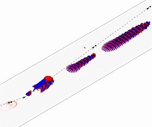
Isovolume pressure disturbance contours are shown in figure 3(a) to illustrate the particle-induced flow field at five time instances I–V, which relate to before, near and after particle impingement. It was previously demonstrated in Browne et al. (Reference Browne, Hasnine, Russo and Brehm2020b) that the PSIC approach in combination with an appropriate particle drag model used here is able to capture the main features of the disturbance flow field. The particle travels with relatively constant velocity in the free stream. Once it enters the boundary layer, the flow regime changes from subsonic to supersonic around the particle and the relative Mach number reaches a peak value of ${M}_{max}\approx 2.5$ as shown in figure 3(b). A shock forms ahead of the particle with high pressure in front as well as a low pressure region in the wake. Figure 4 shows the total drag force, $D_p$, and the drag coefficient, $C_d$, together with snapshots of the disturbance pressure field at four time instances during the time the particle is entering and leaving the boundary layer. The drag force was obtained from the local flow conditions and drag coefficient correlations as described in § 2.2. As the particle enters the boundary layer the drag coefficient, drag force and relative Mach number (see figure 3b) of the particle increase substantially. Around the peak value in the drag coefficient the particle breaks through the sound speed barrier and the sonic boom impinges on the wall as highlighted in figure 5(a). The shock structure around the particle can be seen in figure 4(c,d). The drag force reaches its peak value by the time the particle touches the wall. The particle impingement generates disturbances in the boundary layer with a large spectral content. A region of acoustic waves forms downstream of the particle impingement location, which decays rapidly. Away from the impingement region, a wavepacket is formed that propagates in the downstream direction, experiencing exponential growth. The aim of the current work is to study the modal contributions of the discrete and continuous branches to the overall development of the disturbance flow field.

Figure 3.

(a) Contours of pressure disturbance ($p/\rho _\infty U_\infty ^{2}$) flow field for a Mach 5.35 flat plate boundary layer at five time instances: (I) before impingement, (II) near the impingement location and (III, IV, V) after impingement. (b) Particle Reynolds number and Mach number. Vertical solid line and dashed lines mark the position when the particle enters and leaves the boundary layer and (c) the pressure field in the cut plane. (Particle size not to scale and $\tau$ is based on the particle position.)

Figure 4.

(a) Drag coefficient, $C_d$, and drag force, $D_p$, of the particle, and (b–e) pressure disturbance flow field at four time instances marked as vertical green dashed lines in figure (a). The vertical red solid line marks the position of the particle entering and the red dashed line marks the particle leaving the boundary layer, respectively. The red lines in figures (b–e) mark the boundary-layer edge.

Figure 5.

Space–time diagram of wall pressure amplitude ($|p_w|/(\rho _\infty U^{2}_{\infty })$) at different $\beta$ (non-dimensionalized by $H(x=0.138\,{\rm m})$) in time. Vertical dashed lines mark the particle impingement location; horizontal solid lines, from bottom towards top, mark the time when the particle enters the boundary layer (BL), collides at the wall and leaves the boundary layer (BL), respectively. The symbol $\bigcirc$ marks the shock wave reaching the wall, $\oplus$ marks the flow feature generated through mean flow distortion and $\otimes$ marks the acoustic wave reaching the wall. The solid lines in plot (a) correspond to the minimum phase speed with $C_{r_{min}}=0.82$ (blue line), the maximum phase speed with $C_{r_{max}}=0.95$ (green line), the minimum group velocity with $C_{g_{min}}=0.5$ (red line) and the maximum group velocity with $C_{g_{max}}=0.63$ (yellow line). Results are shown for (a) $\beta =0$, (b) $\beta _{x/H=1374}=0.28$.

To analyse the temporal and spatial evolution of the wall pressure signature, the unsteady wall pressure signal is Fourier transformed in the spanwise direction. Figure 5(a,b) shows space–time diagrams of the wall pressure amplitude for $\beta =0$ and $\beta =0.28$. The times (on the vertical axis) when the particle enters the boundary layer, collides with the wall and leaves the boundary layer are marked as black horizontal solid lines. Already before the particle enters the boundary layer an acoustic wave travelling upstream of the particle generates a pressure disturbance on the wall (marked as $\otimes$). The acoustic wave was introduced when the particle was released in the flow. Similarly a wave field would be generated as a particle travels through a shock front upstream of a hypersonic vehicle. As the particle enters deeper into the boundary layer, the flow around it becomes supersonic that leads to the formation of a shock front. The shock wave extends all the way to the wall where it reflects and generates large wall pressure fluctuations even before the particle impinges on the wall (marked as $\bigcirc$). It has also been noted in additional simulations not shown here that even when smaller particles do not impinge on the wall and they barely graze the boundary-layer edge, a pressure disturbance field can be generated inside the boundary layer. This type of receptivity mechanisms is, however, beyond the scope of the current work. The particle traversing through the boundary layer and impinging on the surface causes a mean flow distortion of the boundary layer with a relaxation time that is several times larger than it takes the particle to enter and exit the boundary layer. In figure 5(a) the associated flow feature in the $x-t$ diagram extends vertically from the impingement location into the free stream (marked as $\oplus$). The wall pressure disturbance plot for a spanwise wavenumber of $\beta =0.28$ in figure 5(b) shows non-negligible amplitude levels at spanwise wavelengths significantly larger than the size of the particle. This means that the spanwise extent of the pressure field generated in the vicinity of the impingement location is many times larger than the size of the particle itself. This low wavenumber content decays, however, rapidly in the downstream direction. This behaviour is expected as the following LST analysis results will show that disturbances at these wavelengths are generally damped for the current flow conditions. The pressure field emanating away from the impingement region travels with different propagation speeds following different dispersion relationships based on the nature of the wave field. The envelope of the pressure disturbance field can be bounded by the FA speed with $C^+_r = 1+1/{M}$. The maximum and minimum phase speeds are $C_{r_{max}}=0.95$ and $C_{r_{min}}=0.82$ and they are marked by green and blue solid lines, respectively. The second-mode dominated wavepacket dictating the flow field further downstream of the impingement location will propagate with the group velocity. The line for $C_r=1-1/M=0.81$ is slightly offset to distinguish it from the $C_{r_{min}}=0.82$ line. The maximum and minimum group velocities at the maximum amplification rate (throughout the domain) are $C_{g_{max}}=0.63$ and $C_{g_{min}}=0.5$, respectively. The yellow and red solid lines in figure 5(a) mark the maximum and minimum group velocities, respectively. The region with high fluctuation amplitudes seem to closely follow the group velocity that was predicted with LST. Moreover, the hump of the wavepacket from the simulation is compared with the LST calculations in figure 6. In LST the trajectory of the wavepacket hump is obtained by calculating the group velocity, $C_g$, following the $C_g={{\rm d} x}/{\rm d}t$ relation. The hump trajectory extracted from the DNS and the trajectory calculated with the group velocity obtained from the LST analysis are in close agreement.

Figure 6.

Wave-hump trajectory extracted from the DNS and LST prediction.

Next, we analyse the characteristics of the disturbance field introduced through particle impingement and what fractions of the disturbance energy will arrive in the second-mode dominated wavepacket. Figure 7(a) shows the development of the $\beta =0$ disturbance amplitude in the downstream direction. As the wavepacket propagates further downstream, the high pressure amplitude region shifts from higher to lower frequencies following an inverse proportional relationship to the boundary-layer height. Far from the particle impingement location, the pressure amplitude plot is in agreement with the LST results (figure  7b). The neutral curves are included as blue solid lines for the unstable mode S (here, the second Mack mode). It should be noted here that the LST predictions are based on the parallel flow assumption; thus, may not perfectly match the DNS results. The peak values of the wall pressure amplitude is within the second-mode frequency range as predicted by LST with the maximum pressure amplitude occurring near the second branch of the neutral curve at the downstream locations. The LST analysis shows that both first and second instability modes are expected in the flow field, as shown in figure 7(c). To compare the pressure amplitude development in the downstream direction, pressure amplitude curves are plotted at three distinct frequencies $F=7.543\times 10^{-5}, 7.023\times 10^{-5}$ and $6.502\times 10^{-5}$ and compared with the LST computations in figure 7(d). In the unstable flow region there is good agreement between the DNS and LST results. The first-mode contribution is not noticeable in the amplitude plots in figure 7(a). This also suggests that far from the particle impingement location the flow field is dominated by the discrete unstable second mode S. The discrepancies near the particle impingement location indicate that the contributions from other discrete modes and continuous branches are not negligible at upstream locations and these contributions can influence the downstream development of the flow field.

Figure 7.

(a) Wall pressure FFT amplitude plot at $\beta =0$. The horizontal dashed lines mark the frequencies at which amplitude curves are extracted for comparison, blue lines mark the neutral curves for the second mode. The vertical red dashed line marks the particle impingement location, (b) amplitude plot obtained from LST, (c) growth rate at $\beta =0$ and (d) amplitude development for different frequencies for numerical simulation and LST. Symbols and lines, which respectively represent FFT and LST data, denote the following: ($\square$, solid line) $F=7.543\times 10^{-5}$, ($\bigcirc$, dashed line) $7.023\times 10^{-5}$ and ($\Diamond$, dashed-dotted line) $6.502\times 10^{-5}$.

A more detailed overview of the pressure field in the vicinity of the particle impingement location can be obtained from the wall pressure amplitudes in the $F$-$\beta$ spectra as shown in figure 8(a–d) for four streamwise locations, $x/H$. The $F$-$\beta$ spectrum right at the particle impingement location is shown in figure 8(a). The neutral curves for the second mode are again included as blue solid lines. A wide range of frequencies and wavenumbers are introduced by the particle impingement with a large pressure amplitude within the range $0\leq \beta <0.5$ and up to $F\approx 2\times 10^{-4}$. The largest amplitudes are introduced for $\beta =0$ at very low frequencies around $F\approx 2\times 10^{-5}$ and higher frequencies around $F \approx 16 \times 10^{-5}$ as well as a strong oblique contribution at around $F\approx 15 \times 10^{-5}$ and $\beta =0.32$. The higher frequency content persists near the impingement location at $x/H=1432$ with main contributions from around four regions marked (with 1, 2, 3/4 and 5) in figure 8(b) that will be analysed in more detail employing BOD. Further downstream the 2-D mode with $\beta =0$ dominates and amplitude peaks can be found at frequencies that would be expected from LST predictions in figure 8(c,d). Furthermore, the peak shifts from the lower branch of the neutral curve towards the upper branch (as is expected from LST) in the downstream direction as disturbances are exponentially amplified.

Figure 8.

Wall pressure amplitude ($|p_w|/(\rho _\infty U^{2}_{\infty })$) in $F-\beta$ diagram. Here ‘+, red’ marks the cases considered for reconstruction in § 6.3. Blue lines mark the neutral curves for the second mode. Results are shown for (a) $x_{pc}/H=1374$, (b) $x/H=1432$, (c) $x/H=1525$, (d) $x/H=2517$.

The wall-normal amplitude distributions of pressure, streamwise velocity, wall-normal velocity and temperature of the 3-D disturbance flow field are shown at three downstream locations, $x/H=1374$, $1432$ and $2517$ in figure 9(a–l) for $\beta =0$. The first two locations ($x/H=1374$ and $1432$) are selected to provide an overview of the disturbance flow features in the vicinity of the impingement location and the location further downstream ($x/H=2517$) shows the flow field in a region dominated by mode S. At the impingement location ($x_{pc}/H=1374$), the largest pressure amplitudes are introduced at low frequencies ($F<9\times 10^{-5}$) extending throughout the boundary layer. Interestingly, the largest pressure peak is not obtained at the wall right at the impingement location. At the impingement location, no consistent trends among the different flow quantities with respect to the dominant frequency ranges can be observed. The four chosen flow quantities can be divided into two groups based on their spectral content where pressure and wall-normal velocity display similar frequency characteristics and streamwise velocity and temperature form the other group. Roughly only a three boundary-layer thickness away from the particle impingement location at $x/H=1432$ (figure 9e–h), a second region with large amplitudes in pressure appears around $F\approx 1\times 10^{-4}$ below the sonic line ($x/H=5.3$) (marked as a dashed dotted line in the plots). For the streamwise velocity component and the temperature field, the peak values are contained within the boundary layer while the wall-normal velocity and pressure distribution show a low frequency peak outside of the boundary layer at $x/H=1374$ and $1432$. This peak is associated with acoustic waves travelling outside the boundary layer as will be demonstrated when reconstructing the flow field. In the vicinity of the impingement location at $x/H=$1374 and 1432, the streamwise velocity and temperature disturbances are dominated by low frequency content mainly inside the boundary layer. A possible explanation for this could be a transient growth-like mechanism that is active and manifests itself in the streamwise velocity and temperature disturbances. Similar observations with a more prominent non-modal growth mechanism was observed for particle impingement on a blunt cone in Russo et al. (Reference Russo, Hasnine and Brehm2021) consistent with optimal growth results obtained in Paredes et al. (Reference Paredes, Choudhari, Li, Jewell and Kimmel2019). The disturbance flow field spectra at $x/H=2517$, further downstream of the particle impingement location, are very different from those closer to the impingement location. The spectra for all flow quantities are dominated by a narrow frequency band that appears to be associated with the exponentially amplified mode S in this region marked with blue dashed lines. Furthermore, as expected from the LST theory, the pressure distribution peaks right at the wall and the temperature distribution peaks right below the boundary-layer edge. Interestingly, the largest pressure peak is not obtained at the wall right at the impingement location.

Figure 9.

Disturbance flow frequency spectra in the wall-normal direction at $\beta =0$ for (a,e,i) pressure, (b, f,j) streamwise velocity, (c,g,k) wall-normal velocity and (d,h,l) temperature at three streamwise positions. The vertical dashed red line marks the boundary-layer height, the vertical dashed-dotted red line marks the position of the sonic line and horizontal blue dashed lines mark the second-mode frequency range. Results are shown for (a) $|p|$, $x_{pc}/H=1374$; (b) $|u|$, $x_{pc}/H=1374$; (c) $|v|$, $x_{pc}/H=1374$; (d) $|T|$, $x_{pc}/H=1374$; (e) $|p|$, $x/H=1432$; ( f) $|u|$, $x/H=1432$. (g) $|v|$, $x/H=1432$; (h) $|T|$, $x/H=1432$; (i) $|p|$, $x/H=2517$; (j) $|u|$, $x/H=2517$; (k) $|v|$, $x/H=2517$; (l) $|T|$, $x/H=2517$.

Next, instead of considering different components of the state vector where these components provide widely different distributions, a scalar quantity weighing the individual contributions based on a consistent energy norm will be used. In order to measure the energy contained within the disturbance flow field several energy norms are available. Here, the energy norm by Chu (Reference Chu1965) for perturbations within temporal stability analysis has been adopted in the form

(5.1)\begin{equation} E_{dist} = \frac{1}{2}{\bar \rho}(\langle\,{\breve u},{\breve u}\rangle+\langle\,{\breve v},{\breve v}\rangle+\langle\,{\breve w},{\breve w}\rangle)+\frac{1}{2}\frac{{\bar a^2 \langle\,{\breve \rho},{\breve \rho}\rangle}}{\gamma {\bar \rho}}+\frac{1}{2}\frac{{\bar \rho c_v \langle\,{\breve T},{\breve T}\rangle}}{\bar T}, \end{equation}

where ${\bar a}^2 = {\bar T}/{\mathrm {M}^2}$ and $c_v = [\gamma (\gamma -1) \mathrm {M}^2]^{-1}$, ${\bar \rho }$ and ${\bar T}$ are the mean flow density and temperature, $({\breve u},{\breve v}, {\breve \rho },{\breve T}) \in \mathbb {C}$ are the Fourier transformed spectra for disturbance streamwise velocity, wall-normal velocity, density and temperature, the inner product is given by $\langle \,{\breve u},{\breve u}\rangle \equiv ({\breve u}^*{\breve u} + {\breve u}{\breve u}^*)/2$, $(\boldsymbol {\cdot })^*$ stands for the complex conjugate and $\gamma =1.4$ is the specific heat ratio. All flow parameters are non-dimensionalized by free-stream quantities ($U_\infty,\rho _\infty, T_\infty$). It is also known as ‘Mack norm’ because it was used in Mack's comprehensive report (Mack Reference Mack1969) on the stability of boundary layers. (The energy norm (5.1) was independently derived also in Hanifi, Schmid & Henningson (Reference Hanifi, Schmid and Henningson1996).) This norm is also used for spatially growing perturbations in spite of an absence of reasoning for its use.

The disturbance energy spectra are shown in figure 10(a–f) for three downstream locations $x/H=1374,1432$ and $2517$ as well as two spanwise wavenumbers $\beta$. At the impingement location $x_{pc}/H=1374$, the two main peaks of the disturbance energy are found just above the wall and below the boundary-layer edge, similar to the peaks in the temperature and wall-normal velocity of the disturbance flow field for $\beta =0$ and $\beta =0.055$. The low frequency peak extends throughout the boundary layer which suggests its association with mean flow distortion. Shortly downstream of the impingement location at $x/H=1432$ the spectra look already distinctly different from the spectra at $x_{pc}/H=1374$. The local maxima in the disturbance energy spectra are spatially localised such that they will dominate only parts of the boundary layer. Moreover, the disturbance energy peaks outside the boundary layer at $y/H=33$, suggesting that a considerable amount of the disturbance energy introduced by the particle impingement is carried away by acoustic waves. For the downstream location at $x/H=2517$, the energy peak is found to occur at a higher frequency (between $5\times 10^{-5}<{F}<1\times 10^{-4}$) for $\beta =0$ falling within the second-mode dominated frequency range. An additional low frequency peak appears at a higher spanwise wavenumber $\beta =0.058$ in figure 10( f), suggesting a considerable low frequency contribution from oblique waves. These low frequency peaks are associated with the presence of the first mode as indicated by frequency ranges marked in figure 10( f).

Figure 10.

Frequency spectra of disturbance energy at three different streamwise locations and two spanwise wavenumbers. The vertical dashed red line marks the boundary-layer height, the vertical dashed-dotted red line marks the position of the sonic line, horizontal blue dashed lines mark the second-mode frequency range and horizontal green dashed lines mark the first-mode frequency range. Results are shown for (a) $x_{pc}/H = 1374, \beta = 0$; (b) $x/H = 1432, \beta =0$; (c) $x/H = 2517, \beta =0$; (d) $x_{pc}/H = 1374, \beta = 0.055$; (e) $x/H = 1432, \beta =0.05$; ( f) $x/H = 2517, \beta =0.058$.

Figure 11(a–c) shows the peak values of disturbance energy in the wall-normal direction at three streamwise locations $x/H=1374, 1432$ and $2517$, which is defined as

(5.2)\begin{equation} E_{max}(x,F) = \max_{0\le y\le L_y} \left( E(x,y,F) \right). \end{equation}

Figure 11.

Maximum disturbance energy, $E_{max}(x,F)$ as in (5.2), in the wall-normal direction. The blue lines mark the neutral curves for the second mode. Results are shown for (a) $x_{pc}/H=1374$, (b) $x/H=1432$, (c) $x/H=2517$.

It was observed that an L2 integral based norm provides a nearly identical distribution as the maximum energy norm used here. At the impingement location, the disturbance energy peak is contained in the lower frequency range $0< F<2\times 10^{-5}$ and within $0 \leq \beta \leq 0.6$. A lower amplitude region can be detected within the ($F$,$\beta$) range associated with the second mode. Similarly, just a few boundary-layer thicknesses downstream, at $x/H=1432$, the low frequency range is still dominant and no significant peaks can be detected in the second-mode ($F,\beta$) range. Far from the particle impingement region, the disturbance energy peak is found close to the second-mode neutral curves ($6.45\times 10^{-5} < F < 7.57\times 10^{-5}$) as well as for spanwise wavenumber and frequency ranges associated with the first mode. Hence, the disturbance energy at this location is contributed by the first and second modes. It is important to note that the presence of the first mode could not be detected in the wall pressure spectra in figure 8(b) because the wall pressure signature highlights the second mode more than the first mode due to its inherent eigenmode structure.

Although the introduced disturbance flow field is highly three dimensional in nature near the impingement location, the 2-D mode ($\beta =0$) dominates in the region further downstream. Near the impingement location, the frequency–wavenumber spectra indicate the presence of a wide range of modes from both the discrete and continuous spectra; most of which, however, decay rapidly in the downstream directions or affect the flow field outside the boundary layer. The disturbance energy spectra follow the trend as seen in the frequency–wavenumber spectra, i.e. the disturbance energy is concentrated at a lower frequency region near the impingement location and the peak disturbance energy region shifts to higher frequencies in the downstream direction. Lower magnitudes of disturbance energy are observed at larger $\beta$ due to the presence of weak oblique waves that are amplified due to first-mode growth as verified in figure 7(c).

6. Projection of the 3-D disturbance flow field onto LST eigenmodes

In order to project the disturbance flow field onto the eigenmodes, the BES requires the solution of the direct and adjoint EVPs. The BES can be written as

(6.1) \begin{gather} \left. \begin{gathered} \frac{\partial}{\partial y}\left(\boldsymbol{\mathsf{L}}_0\frac{\partial \boldsymbol{A}_{\alpha\beta}}{\partial y} \right)+\boldsymbol{\mathsf{L}}_1\frac{\partial \boldsymbol{A}_{\alpha\beta}}{\partial y} - \boldsymbol{\mathsf{H}}_1\boldsymbol{A}_{\alpha\beta}- {\rm i}\alpha\boldsymbol{\mathsf{H}}_2{\boldsymbol{A}_{\alpha\beta}}-{\rm i} \beta \boldsymbol{\mathsf{H}}_3 \boldsymbol{A}_{\alpha\beta}=0,\\ \text{y} = 0: \ A_{\alpha\beta 1}=A_{\alpha\beta 3}=A_{\alpha\beta 5}=A_{\alpha\beta 7}=0,\\ y \rightarrow \infty : \ |A_{\alpha\beta i}| < \infty, \text{ and} \end{gathered} \right\} \end{gather}

(6.2) \begin{gather} \left. \begin{gathered} \frac{\partial}{\partial y}\left(\boldsymbol{\mathsf{L}}^T_0\frac{\partial \boldsymbol{B}_{\alpha\beta}}{\partial y} \right)-\boldsymbol{\mathsf{L}}^T_1\frac{\partial \boldsymbol{B}_{\alpha\beta}}{\partial y} - \boldsymbol{\mathsf{H}}^T_1\boldsymbol{B}_{\alpha\beta}- {\rm i}\alpha\boldsymbol{\mathsf{H}}^T_2{\boldsymbol{B}_{\alpha\beta}}-{\rm i} \beta \boldsymbol{\mathsf{H}}^T_3 \boldsymbol{B}_{\alpha\beta}=0,\\ \text{y} = 0: \ B_{\alpha\beta 2}=B_{\alpha\beta 4}=B_{\alpha\beta 6}=B_{\alpha\beta 8}=0,\\ y \rightarrow \infty : \hskip 5pt |B_{\alpha\beta i}| < \infty, \end{gathered} \right\} \end{gather}

where ${\boldsymbol {A}}_{\alpha \beta }$ and ${\boldsymbol {B}}_{\alpha \beta }$ are the solutions to the direct and adjoint EVPs. The orthogonality relation between the eigenfunctions ${\boldsymbol {A}}_{\alpha \beta }$ and ${\boldsymbol {B}}_{\alpha \beta }$ is given by

(6.3) \begin{equation} \langle \boldsymbol{\mathsf{H}}_2{\boldsymbol{A}}_{\alpha\beta},{\boldsymbol{B}}_{\alpha^* \beta}\rangle\equiv \int^\infty_0(\boldsymbol{\mathsf{H}}_2{\boldsymbol{A}}_{\alpha\beta},{\boldsymbol{B}}_{\alpha^* \beta})\,\text{d}y=\varGamma \Delta_{\alpha\alpha*}, \end{equation}

where $\varGamma$ is a normalization constant and $\Delta _{\alpha \alpha ^*}$ is the Kronecker delta if any of $\alpha$ or $\alpha ^*$ is a discrete mode. However, $\Delta _{\alpha \alpha ^*}$ is the Dirac delta if $\alpha$ and $\alpha ^*$ are from the continuous spectra. When ${\boldsymbol {A}}_{\alpha \beta }$ and ${\boldsymbol {B}}_{\alpha \beta }$ are determined, the projection of the disturbance flow field on discrete $\alpha$ can be determined, given that $\boldsymbol {A}(x,y,z)$ is known, from the following relation:

(6.4) \begin{equation} \hat{\boldsymbol{A}} =\frac{\langle \boldsymbol{\mathsf{H}}_2\boldsymbol{A},{\boldsymbol{B}}_{\alpha\beta}\rangle}{\langle \boldsymbol{\mathsf{H}}_2{\boldsymbol{A}}_{\alpha\beta}, {\boldsymbol{B}}_{\alpha\beta}\rangle}{\boldsymbol{A}}_{\alpha\beta}. \end{equation}

Here ${\langle \boldsymbol{\mathsf{H}}_2\boldsymbol {A},{\boldsymbol {B}}_{\alpha \beta }\rangle }/{\langle \boldsymbol{\mathsf{H}}_2{\boldsymbol {A}}_{\alpha \beta },{\boldsymbol {B}}_{\alpha \beta }\rangle }$ is referred to as the amplitude of mode $\alpha$ or coefficient of projection (COP) (Gaydos & Tumin Reference Gaydos and Tumin2004). The projections on continuous modes are carried out by first projecting the FFT of the disturbance flow on different modes within a range of continuous spectra parameter, $k$. Then the projected profile is constructed by performing an integration over the $k$ range. Finally, the solution of the linearized Navier–Stokes equations in the frequency domain can be expressed as a superposition of normal modes from the discrete and continuous branches

(6.5) \begin{equation} \boldsymbol{A_\beta}(x,y) = \underbrace{\sum_{d} {\chi_d\boldsymbol{A}_{\alpha_d}}(y) {\rm e}^{{\rm i}\alpha_dx}}_{\textit{Contribution from discrete spectrum}} +\underbrace{\sum_{c} \int_0^\infty {\chi_c(\textit{k})\boldsymbol{A}_{\alpha_c}}(y) {\rm e}^{{\rm i}\alpha_c(\textit{k})x}\,{\rm d}k}_{\textit{Contribution from the continuous branches}}, \end{equation}

where $d$ and $c$ refer to the ranges of discrete modes and continuous branches, respectively. The values of $\chi _d$ and $\chi _c$ can be obtained from the BES. The modes associated with continuous spectra have eigenfunctions oscillating outside of the boundary layer as $\exp (\pm \textrm {i} k y)$, where $k$ is a real parameter (see figure 2b). This is in contrast to the discrete modes that decay exponentially outside the boundary layer (see figure 2b).

In this section the projection of the 3-D unsteady disturbance flow field onto the LST eigenmodes is discussed. The eigenmodes from the discrete and continuous branches affect the evolution of the disturbance flow field in different ways. To understand the initiation of eigenmodes within the receptivity process and the subsequent development of mode S inside the boundary layer, the disturbance flow field is first projected onto the most dominant discrete eigenmode S. Then the projection on the continuous spectra is presented to discuss the disturbance flow development outside the boundary layer in the free stream. Lastly, the projection on the full discrete and continuous spectra is considered to understand the spectral characteristics to the disturbance flow field. It will also be demonstrated that the disturbance flow field can be fully reconstructed with a combination of continuous and discrete modes.

6.1. Projection of disturbance flow field on discrete mode S

The 3-D disturbance flow field obtained from the simulations is projected on the unstable discrete mode S using BES. The second mode, here associated with mode S, typically contains moderate frequencies unlike the first mode that appears at relatively low frequency. The current study focuses on mode S because it reaches larger N factors than the first mode. The quasi-parallel flow assumption has been adopted within the current analysis as introduced in § 3.

Figures 7(a) and 12(a) display the Fourier wall pressure amplitude distribution and its projection of wall pressure on mode S at $\beta =0$, respectively. The spectra in figures 7(a) and 12(a) can be directly compared with each other to obtain an idea about the relative contribution of mode S to the disturbance flow field. In the region downstream of the impingement location the pressure contours are nearly identical, which means that mode S is dominating the disturbance flow field in this region. The projected wall pressure spectrum is close to the expected frequency range following pure second-mode growth. Some differences between the projected and original pressure amplitude spectra are observed near to the impingement location where mode S has a lower amplitude. Next, amplitude curves and projection ratios ($\psi = P_{proj.}/P_{fft}$) are compared for three frequencies, $F=7.543\times 10^{-5},7.023\times 10^{-5}$ and $6.502\times 10^{-5}$, in figures 12(b) and 12(c), respectively. A general trend towards the projection ratios approaching $\psi =1$ in the exponential growth regime is apparent, i.e. when the disturbances cross branch I of the neutral curve predicted by LST. Branch I/II locations are marked as vertical dashed lines in figure 12(c). The results suggest that once the disturbance flow reaches branch I the unstable mode S becomes dominant. Here, the amplitude curves follow the LST prediction and the projection ratio is close to one. For the highest frequency $F=7.543\times 10^{-5}$ shown here, the projection coefficient starts to move away from $\psi =1$ when approaching the second branch. The differences near the particle impingement location can be attributed to considerable contributions from the continuous branch as well as other stable discrete modes near the impingement location. Far from the particle impingement location and inside the unstable flow region, the amplitude curves from FFT, LST and projection on mode S are in close agreement and the projection ratio is close to unity. Balakumar & Malik (Reference Balakumar and Malik1992) also made similar observations when considering a point disturbance source in a $M=2$ and $M=4.5$ flat plate boundary-layer flow. While they did not attempt to reconstruct the flow field in the vicinity of the source region they showed that the disturbance flow field can be described very accurately far from the disturbance source by considering only the unstable modes.

Figure 12.

(a) Wall pressure disturbance flow field projected onto mode S at $\beta =0$. Blue lines mark the neutral curves for the second mode, (b) amplitude curves for different frequencies and (c) projection ratio, $\psi$, where the vertical dashed lines represent the first (I) branch and the vertical dashed-dotted line represents the second (II) branch. Symbols used denote the following: ($\blacksquare$; $\square$; solid line) $F_1=7.543\times 10^{-5}$, (${\unicode{x25CF}}$; ${$_{\bigcirc}$}$; dashed line) $F_2=7.023\times 10^{-5}$ and ($\blacklozenge$; $\lozenge$; dashed-dotted line) $F_3=6.502\times 10^{-5}$. Filled symbols represent projection on mode S, hollow symbols represents FFT and lines represent LST.

The FFT of the disturbance pressure field and its projection on mode S are also shown in the $F$-$\beta$ plane in figure 13(a,c). The original frequency–wavenumber spectra are available for comparison in figure 8(a,b). As the wavepacket travels in the downstream direction, the peak of the wall pressure projection on mode S shifts from the lower branch towards the upper branch of the neutral curve as LST would predict. The large differences in the spectra near the impingement location at $x_{pc}/H=1374$ (figure 13a) and $1432$ (figure 13c) are expected as the contributions from other modes are still significant at these locations. The projection ratios shown in figure 13(b,d) highlight the region in the spectrum where the second mode is activated. The dashed contour lines of the original wall pressure spectra were included in figure 13(a,c) to provide an overview of the significant contributions from other discrete and continuous modes that are present in the initial disturbance flow field. The projection ratio in figure 13(d) indicates that the first mode is also triggered through particle impingement with higher amplification rates at oblique angles.

Figure 13.

Fourier transformed disturbance wall pressure projected onto mode S: (a,c) contour plots. Dashed contour lines represent the disturbance flow FFT and (b,d) projection ratio. Results are shown for (a) $x_{pc}/H=1374$, (b) $x_{pc}/H=1374$, (c) $x/H=1432$, (d) $x/H=1432$.

The receptivity coefficient is calculated along the lower neutral branch I for different wave angles, $\theta =tan^{-1}(\beta /\alpha _r)$, in the form

(6.6)\begin{equation} C_{recep} = \frac{|P_{w_S}|}{\rho U^2_{rel}}, \end{equation}

where $|P_{w_s}|$ is the wall pressure amplitude projected on mode S, $\rho$ is the fluid density and $U_{rel}$ is the relative velocity of the particle. The receptivity coefficient, $C_{recep}$, along the lower neutral branch is provided in figure 14 for two different downstream locations with $x_{pc}/H=1374$ and $x/H=1432$. The receptivity coefficient is fairly constant until a wave angle of $\theta \approx 30^{\circ }$.

Figure 14.

Receptivity coefficient for different wave angles, $\theta =\tan ^{-1}(\beta /\alpha _r)$, at the lower neutral branch.

It is common practice in DNS studies of boundary-layer transition scenarios to simply use the wall pressure signature to analyse the transition process. Hereby, it is assumed that the disturbance pressure peaks occur at the wall, which is the case for first- and second-mode disturbance waves; thus, tracking wall pressure is equivalent with applying the maximum or $L_\infty$ norm. The wall-normal distributions of the different disturbance flow quantities were shown in figure 9. The projections on mode S are displayed in figure 15. Comparing the original disturbance flow signals with their projections on mode S demonstrates that the low frequency contributions, not associated with the first or second mode, are the main contributors to the disturbance flow field in the vicinity of the impingement location. As mode S experiences exponential growth and begins to dominate the downstream development of the disturbance flow field, good agreement with the original data in figure 9 is obtained. The amplitude peaks for the different flow quantities are observed around the frequency range of mode S. The projections on mode S at $x/H=2517$ closely represent the spectral content of the disturbance flow field in figure 9(i–l), suggesting significant contributions from mode S at this location.

Figure 15.

Disturbance flow frequency spectra projected on mode S at $\beta =0$ versus wall-normal direction for (a,e,i) pressure, (b, f,j) streamwise velocity, (c,g,k) wall-normal velocity and (d,h,l) temperature at three streamwise positions. The vertical dashed line marks the boundary-layer height, the vertical dashed-dotted line marks the position of the sonic line and horizontal blue dashed lines mark the neutral curves for the second mode. Results are shown for (a) $|p|$, $x_{pc}/H=1374$; (b) $|u|$, $x_{pc}/H=1374$; (c) $|v|$, $x_{pc}/H=1374$; (d) $|T|$, $x/H=1374$; (e) $|p|$, $x/H=1432$; ( f) $|u|$, $x/H=1432$; (g) $|v|$, $x/H=1432$; (h) $|T|$, $x/H=1432$; (i) $|p|$, $x/H=2517$; (j) $|u|$, $x/H=2517$; (k) $|v|$, $x/H=2517$; (l) $|T|$, $x/H=2517$.

The contribution of mode S throughout the boundary layer at different downstream locations can be assessed by comparing the original amplitude distributions and their projections on mode S in figure 16(a–i). Streamwise velocity, pressure and temperature profiles are provided in figure 16(a–i) for $\beta =0$ at $F=7.543\times 10^{-5}$ for three different streamwise locations. The discrepancies between the disturbance flow FFT and projection on mode S observed in the $F$-$\beta$ plane for wall pressure are also present in their profiles near the particle impingement location. At the impingment location, the FFT distributions for the different disturbance flow quantities are distinctly different from the projected results. The peak values are about an order of magnitude smaller with $(P_{fft,max})/(P_{proj.,max})\approx 10.02$, $(T_{fft,max})/(T_{proj.,max})\approx 5.62$ and $(u_{fft,max})/(u_{proj.,max})\approx 11$. These ratios give an idea about the small fraction of the disturbance energy that is introduced in mode S during particle impingement. Indeed, the ratio of total maximum disturbance energies ($E_{max}(fft)/E_{max}(proj.)$) is 23.24. The contributions from different discrete and continuous branches of the associated eigenvalue spectrum are identified in § 6.3 for reconstructing the original profiles of the disturbance flow field. Further downstream at $x/H=1670$, while differences in the phase are still present, the disturbance flow profiles tend to follow the general behaviour of mode S. At $x/H=2517$, the disturbance flow profiles are in close agreement with the projection data as one would expect for a flow field that is dominated by mode S.

Figure 16.

Profiles of disturbance flow FFT and its projection on mode S: (a–c) pressure, (d–f) streamwise velocity and (g–i) temperature, for $F=7.543\times 10^{-5}$ and $\beta =0$. Lines and symbols represent FFT and projection on mode S, respectively: solid line and $\blacklozenge$ for $|{\cdot }|$; dashed line and $\bigcirc$ for $\textrm {Re}({\cdot })$; dashed-dotted line and $\Delta$ for $\textrm {Im}({\cdot })$. Results are shown for (a) $x_{pc}/H=1374$, (b) $x/H=1670$, (c) $x/H=2517$, (d) $x_{pc}/H=1374$, (e) $x/H=1670$, ( f) $x/H=2517$, (g) $x_{pc}/H=1374$, (h) $x/H=1670$, (i) $x/H=2517$.

The disturbance energy of the projected disturbance flow field is provided in figure 17(a–f) for the same parameters as in figure 10(a–f). The energy spectra are dominated by the temperature field showing large amplitudes just below the boundary-layer edge. The (stable) low frequency mode S does not contribute significantly to the disturbance flow field at $\beta =0$. The projected energy spectra in figure 10(a–f) contain low frequency peaks at higher spanwise wavenumbers, $\beta$, outside of the range where the second mode is unstable, which explains some peaks in the original energy spectra in figure 10. In summary, the results for the projection on mode S showed that a very small amount of disturbance energy introduced by particle impingement ends up in mode S. The numerical results suggest that most of the disturbance energy is absorbed by the stable discrete modes and modes from the continuous branches, which is analysed in more detail in §§ 6.2 and 6.3. Next, the disturbance flow field is projected on the continuous branch.

Figure 17.

Frequency spectra of disturbance energy projected on mode S at three different streamwise locations and two spanwise wavenumbers ($\beta$). The vertical dashed line marks the boundary-layer height, the dashed-dotted line marks the position of the sonic line and horizontal blue dashed lines mark the unstable frequency range for mode S. Results are shown for (a) $x_{pc}/H = 1374, \beta = 0$; (b) $x/H = 1432, \beta =0$; (c) $x/H = 2517, \beta =0$; (d) $x_{pc}/H = 1374, \beta = 0.055$; (e) $x/H = 1432, \beta =0.05$; ( f) $x/H = 2517, \beta =0.058$.

6.2. Projection of disturbance flow field on the continuous spectra

The continuous spectra are expected to contribute mostly to the development of the disturbance flow field outside the boundary layer as they provide a mechanism to radiate energy away from the boundary layer. Especially near the impingement location continuous branches also provide major contributions to the disturbance flow field throughout the boundary layer, in particular, for low frequencies. The contributions from continuous spectra are analysed for the acoustic branches with $\beta =0$. As the acoustic branch is continuous, superposition of the modal contributions from the acoustic branches needs to be considered for the disturbance flow decomposition. The projection onto the continuous spectra is evaluated for different continuous spectra parameter ’$k$’, also sometimes referred to as the $y$ component of the wavenumber vector. It defines the variations of the acoustic eigenfunctions as $\exp (\pm \textrm {i}ky)$ in the free stream.

The eigenfunctions from the continuous acoustic branch, unlike the discrete modes that decay outside the boundary layer, contribute to the disturbance flow field in the free stream (see figure 2b). The purpose of the analysis in this section is to demonstrate that the disturbance flow field projected on the acoustic branch captures a large portion of the disturbance energy introduced during the particle collision. The disturbance flow field is projected onto the SA and FA modes at low frequency ($F=1.764\times 10^{-5}$) considering $k=0.001-4.0$ with a step size of $\Delta k =0.001$. The amplitude curves of the COP for the SA and FA branches are illustrated in figures 18(a) and 18(b), respectively. Each curve represents a different streamwise location. The maximum amplitude of the COP for the SA and FA branches occur at $x/H=1396$ and $1374$, respectively. The contributions from the FA branch stem from higher $k$ in comparison to the SA branch. Figure 19(a–d) shows the FFT of disturbance flow field and its projection on the SA and FA branches as well as their superposition at $F=1.764\times 10^{-5}$. The acoustic field generated during the particle impingement can be fully reconstructed by considering the acoustic branches. The different contributions from the SA and FA branches can be seen in figures 19(b) and 19(c), respectively. The superposition of the contributions from the SA and FA modes (figure 19d) is able to capture the behaviour of the disturbance flow field outside the boundary layer. Outside the boundary layer, a perfect match is achieved between the original FFT data and the reconstructed pressure field solely considering the contributions from the acoustic branches SA and FA, but inside the boundary layer the other discrete modes need to be included to obtain a closer match.

Figure 18.

Amplitude of the COP for the SA and FA branches at $\beta =0$ and $F=1.764\times 10^{-5}$; (a) SA, (b) FA.

Figure 19.

Pressure amplitude at $\beta =0$ and $F=1.764\times 10^{-5}$ for (a) FFT of disturbance flow field, (b) FFT projected on SA modes ($k=0.001-4.0$), (c) FFT projected on FA modes ($k=0.001-4.0$) and (d) combination of FA and SA ($k=0.001-4.0$). The black line marks the boundary-layer edge. Amplitude normalized by peak value at $x/H=1374$. The Mach angle is 10.7$^\circ$ for the current flow conditions.

6.3. Full reconstruction of the disturbance flow field

In order to identify the contributions from the discrete modes and continuous branches during the receptivity phase, five frequencies, $F$, and spanwise wavenumbers, $\beta$, pairs are considered near to the particle impingement location at $x/H=1432$. Two high frequency cases are taken near to the peaks marked with red crosses in figure 8(b), i.e. case 1 with $F=2.822\times 10^{-4}$ and $\beta =0$ and case 2 with $F=2.315\times 10^{-4}$ and $\beta =0.206$. In addition, cases 3 and 4 consider intermediate frequencies near to the second-mode region at $F=1.014\times 10^{-4}$ and $F=7.938\times 10^{-5}$, respectively, at $\beta =0$ as well as one low frequency case 5 at $F=1.764\times 10^{-5}$ and $\beta =0$ near to the region where the peak occurs outside the boundary layer as, for example, depicted in figure 9(e).

The development of the discrete modes S and F as well as the phase velocities, $C_r=\omega /\alpha _r$, as a function of $F$ at $Re=1432$ and $\beta =0$ are shown in figures 20(a) and 20(b), respectively. The vertical lines in figure 20(a–d) mark the different frequencies considered in this analysis for the reconstruction of the flow field. Multiple F modes exist at higher frequencies. They are denoted as F1, F2 and F3 modes according to their emergence in the eigenvalue spectrum. Mode S synchronizes with the SA branch and mode F synchronizes with the FA branch in the limit of the frequency parameter approaching zero, $F\rightarrow 0$. The phase speeds of the FA and SA branches are marked as horizontal lines at $1+1/M$ and $1-1/M$ in figure 20(b), respectively. Mode S synchronizes with mode F1 at $F\approx 1.07\times 10^{-4}$ and mode F2 at $F\approx 2.88\times 10^{-4}$. The synchronization of mode S with mode F1 gives rise to the unstable second Mack mode. However, no destabilization of the flow is observed for the second synchronization of mode S with mode F2. The synchronization points, however, also provide a mechanism for intermodal energy exchange. For example, at the synchronization point, disturbance energy initially introduced in mode F1 can be passed onto mode S through phase speed matching. This mechanism has been observed in prior receptivity studies when introducing FA disturbances in the presence of an unstable mode S. Similarly, the development of modes S and F and their corresponding phase speeds are shown in figure 20(c,d) as a function of frequency $F$ for oblique waves with $\beta =0.206$ and at $Re=1432$. Mode S synchronizes with mode F1 at $F\approx 1.32\times 10^{-4}$ and mode F2 at $F=3.04\times 10^{-4}$. As seen for $\beta =0$, the modes remain stable after the synchronization occurs. The characteristics of the different modes are in agreement with the simulation results shown in figure 8, where it is observed that the high frequency peaks, both at $\beta =0$ and $\beta \ne 0$, rapidly decay in the downstream direction.

Figure 20.

Development of growth rates of discrete modes ($\alpha _i$) (a,c) and phase velocities for $\beta =0$ with (b) $c_r=\omega /\alpha _r$ and for $\beta = 0.206$ with (d) $c_r=\omega /\sqrt {\beta ^2+\alpha _r^2}$ as a function of $F$ at $Re_H=1432$. The vertical lines mark the frequencies for cases 1, 2, 3, 4 and 5. Here SP denotes synchronization point. Results are shown for (ab) $\beta =0$, (c,d) $\beta =0.206$.

For a more quantitative analysis, the contributions from the discrete modes and continuous branches are determined by computing the projection coefficients and reconstructing the FFT signal for the five cases considered above. The SA and FA branches are discretized within a range of $k=0.001-6.0$ with a step size of $\Delta k=0.001$. The numerical integration of the integral over the continuous acoustic branches considering amplitude distributions, $\hat {\boldsymbol {A}}$, of the SA and FA modes in (6.5) is performed using the trapezoidal method. Figure 21(a–f) shows the COP of the SA and FA branches. The contributions for $k>4$ for cases 1, 2, 4 and 5 are negligible and are therefore not shown here. The FA branch contributes mostly for the higher frequency cases 1, 2, 3 and 4. However, the SA branch, as can be observed in figure 19, dominates the disturbance flow field for the low frequency case 5. Moreover, at low frequency (case 5), the contributions from the FA branch stem from higher $k$ in comparison to the SA branch. It should be noted here that a higher value of $k$ indicates a shorter wavelength.

Figure 21.

Amplitude of the COP for SA, solid line and FA, dashed line branches for the cases 1–5 in (a–e), respectively. Results are shown for (a) $F=2.82\times 10^{-4}, \beta =0$; (b) $F=2.315\times 10^{-4}, \beta =0.206$; (c) $F=1.014\times 10^{-4}, \beta =0$; (d) $F=7.94\times 10^{-5}, \beta =0$; (e) $F=1.76\times 10^{-5}, \beta =0$.

Figures 22–26(a) show the FFT amplitudes of the pressure disturbance flow field and its projection on the discrete modes S and F as well as on the continuous branches SA and FA for the cases 1–5. The corresponding eigenvalue spectra are also shown in figures 22–26(b). The different modes that mostly contribute to the reconstruction of the disturbance flow field are marked with red squares. The eigenvalues of the discrete modes S and F are provided in table 2 for different cases. The eigenvalues are determined by employing the global solver for the cases 1–4. For case 5, the discrete modes are determined by tracking the modes from a higher frequency towards the lower frequency (figure 20a) as the modes are very close to zero and difficult to identify from the eigenvalue spectrum produced by the global solver. For all cases, the vorticity and entropy branches provide negligible contributions to the overall disturbance flow field.

Figure 22.

(a) Case 1 FFT amplitude of disturbance pressure and its projection on discrete modes S and F and continuous branches SA and FA, and (b) eigenvalue spectrum at $x/H=1432$ for $F=2.822\times 10^{-4}$ and $\beta =0$. The vertical dashed line marks the boundary-layer edge.

Figure 23.

(a) Case 2 FFT amplitude of disturbance pressure and its projection on discrete modes S and F and continuous branches SA and FA, and (b) eigenvalue spectra at $x/H=1432$ for $F=2.315\times 10^{-4}$ and $\beta =0.206$. The vertical dashed line marks the boundary-layer edge.

Figure 24.

(a) Case 3 FFT amplitude of disturbance pressure and its projection on discrete modes S and F and continuous branches SA and FA, and (b) eigenvalue spectra at $x/H=1432$ for $F=1.014\times 10^{-4}$ and $\beta =0$. The vertical dashed line marks the boundary-layer edge.

Figure 25.

(a) Case 4 FFT amplitude of disturbance pressure and its projection on discrete modes S and F and continuous branches SA and FA, and (b) eigenvalue spectra at $x/H=1432$ for $F=7.938\times 10^{-5}$ and $\beta =0$. The vertical dashed line marks the boundary-layer edge.

Figure 26.

(a) Case 5 FFT amplitude of disturbance pressure and its projection on discrete modes S and F and continuous branches SA and FA, (b) eigenvalue spectra at $x/H=1432$ for $F=1.764\times 10^{-5}$ and $\beta =0$. The vertical dashed line marks the boundary-layer edge.

Table 2.

Eigenvalues of discrete modes for different cases.

For case 1 shown in figure 22(a), the large fluctuations outside the boundary layer can be attributed to the acoustic branch FA, which is also accompanied by the stable mode F3 decaying slowly outside the boundary layer (as it is still in close vicinity to the FA branch). Contributions from the SA branch are small for this frequency and wavenumber pair. Similar to the oscillations observed outside the boundary layer ($y/H\approx 15-40$), Tumin et al. (Reference Tumin, Wang and Zhong2007) also reported oscillations in a convectively unstable $M=8$ flow over a $5.3^{\circ }$ sharp wedge with wall-blowing suction as a disturbance source. This region of the disturbance flow field is a consequence of the acoustic wave emanating from the boundary layer into the free stream as Mach waves with a Mach angle of 10.7$^\circ$ marked in figure 19. However, inside the boundary layer, the disturbance flow field is dominated by various discrete modes. Modes F2 and F3 provide larger contributions than mode S and a very low contribution from mode F1 is detected close to the wall. Similar observations can be made for case 2 in figure 23(a) considering oblique modes with $\beta =0.206$. For this case, the FA branch dictates the pressure amplitude distribution outside the boundary layer where it almost perfectly matches the disturbance flow field. Inside the boundary layer, the discrete mode F2 dominates that almost perfectly follows the FFT pressure amplitude. The disturbance flow field for this frequency–wavenumber pair can be closely described by only considering the discrete mode F2 and continuous branch FA. The LST analysis results show, however, that these modes are stable and decay in the downstream direction. Although the intermediate frequency cases 3 and 4 in figures 24(a) and 25(a) are very close to each other in the frequency–wavenumber spectrum in figure 8(b), with case 3 contained inside the unstable second-mode region and case 4 just outside, the spectral contributions especially inside the boundary layer are very different. Outside the boundary layer, both acoustic branches contribute to the disturbance flow field and only the FA branch contributes inside the boundary layer. Close to the wall, mode S dominates for case 3 while mode F1 dominates for case 4 and dictates the wall pressure peak observed in the disturbance flow field. The higher receptivity of mode F1 versus mode S may be somewhat surprising as mode F1 is more stable than mode S but the receptivity seems to not be dictated by the growth rate of the modes.

With decreasing frequency, the dominant contributions outside the boundary layer shift from the FA branch to the SA branch. While for all other cases 1-4, the dominant FFT pressure peak was observed at the wall, the pressure peak for case 5 is located outside the boundary layer. The disturbance flow field for case 5 is dominated by the SA branch where the integral contribution from the SA modes almost perfectly matches the peak at $y/H\approx 33$. Some smaller contribution of the SA branch and the discrete mode S can be noted inside the boundary layer. Overall, the contributions from the discrete modes are smaller at this frequency and the disturbance flow field is dominated by the SA branch. This observation is in agreement to the reconstructed pressure field from the acoustic branches displayed in figure 19. It should be noted that, while non-modal growth of disturbances has not been observed in this study it appears to be a possible scenario that can be triggered by particle impingement (see Russo et al. Reference Russo, Hasnine and Brehm2021).

Table 3 lists the projection ratios of wall pressure for the different discrete and continuous modes which can be used to summarise the reconstruction results. For cases 1 and 2, the largest magnitude in the projection ratio is observed for the discrete higher-order Mack mode F2. For case 2, it was even noted that mode F2 alone almost perfectly captures the FFT amplitude distribution. For the intermediate frequency cases 3 and 4, modes S and F1 dominate the disturbance flow field, respectively. For lower frequencies, the acoustic modes seem to dictate the disturbance flow field. Thus, the SA branch provides the largest contribution in terms of the projection ratio for case 5. The relative and maximum errors are computed as following:

(6.7)$$\begin{gather} \text{Rel. error} = \sqrt{\frac{\sum(P_{FFT}-P_{proj})^2}{N \times \text{max}(P_{FFT})}},\quad \text{and} \end{gather}$$

(6.8)$$\begin{gather}\text{Max error} = \frac{|\text{max}(P_{FFT}-P_{proj})|}{\text{max}(P_{FFT})}, \end{gather}$$

where $P_{FFT}$ is the disturbance pressure FFT, $P_{proj}$ is the reconstructed pressure profile from the discrete and continuous modes and $N$ is the number of wall normal points in the amplitude function. The maximum relative error is approximately $2.3\,\%$ for the above cases. The maximum error ranges from $2.6\,\%$ to $8.8\,\%$ for the cases 1–5.

Table 3.

Projection ratios of wall pressure for discrete and continuous modes for cases 1–5. Bold numbers indicate the maximum of the projection ratios of the discrete and continuous modes.

7. Summary and conclusions

Particles are inevitably present in the atmosphere, and they are assumed to be large enough, as measurement data (Turco Reference Turco1992) suggest, to carry sufficient inertia to impinge on the surface of hypersonic vehicles. Although they can then clearly play an important role in the transition process for free flight conditions, this topic has remained largely unexplored in the past. In this paper a detailed analysis of the disturbance field generated by particle impingement on a flat plate boundary-layer flow has been performed with a focus on the receptivity stage. The flow conditions were chosen to be relevant for hypersonic flight where a prototypical second-mode dominated transition scenario can be expected.

Particle impingement generates a complex disturbance flow field with a wide range of frequencies and wavenumbers. The disturbance flow field consists of an assembly of discrete modes (both stable and unstable) mainly active inside the boundary layer and acoustic modes from the continuous FA and SA branches displaying large oscillations outside the boundary layer. Contributions from the two vorticity branches and the entropy branch were found to be negligible. Due to the complex nature of the disturbance flow field, the characterisation of the disturbance flow is highly dependent on what flow quantities are analysed and at what position throughout the boundary layer they are taken. The (integral) energy norm by Chu (Reference Chu1965) was chosen as a representative scalar quantity that can capture the overall dominant dynamics in the disturbance flow field. A large amount of energy is introduced at very low frequency and only a small fraction of the total disturbance energy is projected on to the second mode (here, mode S) at the impingement location. In the vicinity of the impingement location, the peak value of disturbance pressure is at least an order of magnitude higher than the pressure amplitude of mode S. A large portion of the disturbance energy (of low frequency content) is diverted into the free stream, which in the BES is projected on to the continuous SA and FA branches. Some fraction of the disturbance energy (of high frequency content) is absorbed inside the boundary layer into stable discrete modes such as the higher Mack modes, here F2 and F3. These discrete modes then rapidly decay in the downstream direction and are assumed to not play an important role in the transition process. A substantial amount of disturbance energy at high frequency also arrives in the continuous FA modes with large amplitudes not only outside the boundary layer as is typical for the acoustic modes but also with large activation inside the boundary layer.

Although, Forgoston & Tumin (Reference Forgoston and Tumin2005) and others previously showed that an initial value problem can be expanded in BES as a sum of discrete and continuous spectra modes, this property has not been demonstrated for flow fields that are as complex as the particle-induced disturbance flow field analysed here that is characterised by the presence of several discrete modes in combination with active continuous branches. Thus, an important contribution of this work was to demonstrate the full reconstruction of this disturbance flow field by using the BES expansion. Indeed, the acoustic wavefield propagating into the free stream and the wall-normal disturbance profile at different frequency and wavenumber pairs could be fully reconstructed in the vicinity of the impingement location. The BOD was shown to be a powerful tool to gain detailed insight about the complex receptivity mechanisms intrinsic to particle-induced transition.