






1. Introduction
Active flow control (AFC) is an important research area in the field of fluid mechanics, which involves a fluid system being purposely altered by actuators through the exertion of a certain amount of energy input (Collis et al. Reference Collis, Joslin, Seifert and Theofilis2004; Choi, Jeon & Kim Reference Choi, Jeon and Kim2008). Compared with passive control methods that usually involve geometrical modifications, AFC is adaptive and hence can realize more effective control over a much wider operation range. Depending on whether selected signals from the system output are fed back to regulate the actuator(s), AFC can be either open loop or closed loop. Closed-loop control can adjust actuation(s) using feedback signals from sensors, and therefore can automatically operate over a much wider range. The core task of closed-loop control is to design the controller. However, in flow-related systems, the fluid motion is governed by the nonlinear Navier–Stokes equations, and the systems usually involve multiscale and multimodal features, it is thus challenging to judge how the system evolve with certain types of control input. Therefore, the use of classical control theory to design the control law is often unfeasible in AFC. To determine a control law, researchers have developed model-based methods that usually involve certain simplifications, such as linear models (Kim & Bewley Reference Kim and Bewley2007), stochastic models (Brackston et al. Reference Brackston, García de la Cruz, Wynn, Rigas and Morrison2016) and reduced-order models (Rowley & Dawson Reference Rowley and Dawson2017), which have been successfully employed in AFC problems.
Take a classical control problem, vortex-induced vibration (VIV) control, as an example. As one of the most typical problems in both scientific study and engineering applications, VIV occurs when a flow passes a blunt body and asymmetrical vortex shedding appears (Williamson & Govardhan Reference Williamson and Govardhan2004). When the vortex shedding frequency matches the natural frequency of the mass–spring system, more challenging lock-in phenomena occur (Zhang et al. Reference Zhang, Li, Ye and Jiang2015), which can be induced by two different mechanisms – resonance and flutter. Even under a subcritical Reynolds number ( $Re < 47$), when the flow past a stationary cylinder is still steady and stable, VIV can occur (Mittal & Singh Reference Mittal and Singh2005). In addition to understanding the complex underlying physics, suppression of these unwanted phenomena is also of great interest, and AFC is a good solution to this (Hong & Shah Reference Hong and Shah2018).
Until now, most AFC approaches for suppressing VIV have been open loop. For example, Wang et al. (Reference Wang, Tang, Duan and Yu2016a, Reference Wang, Tang, Yu and Duan2017a,Reference Wang, Tang, Yu and Duanb) applied open-loop control strategies to explore lock-on phenomena in VIV control, with a pair of synthetic jets being used to interfere with the vortex shedding process. Utilizing the thermal effect, Wan & Patnaik (Reference Wan and Patnaik2016) studied the effect of body heating on the VIV of a circular cylinder with various mass ratios and structural stiffnesses. Muddada & Patnaik (Reference Muddada and Patnaik2017) used moving-surface boundary-layer control, in which two small cylinders are deployed near the separation point of the main cylinder and their rotational velocities are adjusted to enforce a certain momentum injection. It is also noteworthy that as a simple yet powerful tool for VIV control, rotary control has been utilized in both numerical and experimental environments. For example, Bourguet & Lo Jacono (Reference Bourguet and Lo Jacono2014) studied the effect of rotation rate on the VIV of a circular cylinder at  $Re = 100$, and found that symmetry breaking due to rotary control influenced the higher harmonic fluid force components as well as the phase difference between the fluid force and structural vibration. Du & Sun (Reference Du and Sun2015) used rotary control to suppress the VIV of a circular cylinder, and their results showed that the VIV can be suppressed in the ‘lock-on’ region, where the vortex shedding frequency is locked to the forcing frequency. With a proper forcing frequency and rotational velocity, the VIV amplitude can be suppressed to less than $1\,\%$ of the cylinder diameter. Wong et al. (Reference Wong, Zhao, Lo Jacono, Thompson and Sheridan2018) investigated the flow-induced vibration of a sinusoidally rotating cylinder at a low mass ratio and observed that the vibration frequency may be locked into the forcing rotary oscillation frequency or its one-third subharmonic. The above open-loop control attempts provide basic knowledge about how to mediate the fluid–structure interaction (FSI) process, especially the corresponding physical mechanism (Du & Sun Reference Du and Sun2015). This can be used either to make the vortex shedding frequency deviate from the resonance frequency or to suppress the strength of vortex shedding. In order to achieve the best performance, parameter optimization is usually utilized (Ghraieb et al. Reference Ghraieb, Viquerat, Larcher, Meliga and Hachem2021), which also requires huge cost of computational resources. From the perspective of control theory, open-loop control suffers from varying or perturbed systems, and thus can usually work efficiently only under limited parametric conditions.
To better facilitate VIV control, researchers have also adopted closed-loop control strategies. However, in contrast with the extensive open-loop AFCs, closed-loop controls are quite rare, and mainly apply the classical proportional integral–differential (PID) control scheme or its variants. For example, Zhang, Cheng & Zhou (Reference Zhang, Cheng and Zhou2004) used PID control for VIV suppression under the resonance condition, with a combination of a hot wire sensor and a structural oscillation sensor providing feedback signals to achieve the best VIV control performance, i.e. a VIV amplitude suppression of  $82\,\%$ and drag reduction of $35\,\%$. Wang et al. (Reference Wang, Tang, Yu and Duan2016b) used PID control for VIV suppression, with the flow being mediated by two pairs of windward-suction–leeward-blowing actuators. The results suggest that although the selected control strategies can reach the VIV suppression target, the control performance depends significantly on the choice of control parameters. Vicente-Ludlam, Barrero-Gil & Velazquez (Reference Vicente-Ludlam, Barrero-Gil and Velazquez2018) investigated closed-loop VIV control in an experimental environment, and a rotation law proportional to the cylinder's displacement was found to enhance the vibration while another rotation law proportional to the cylinder's transverse velocity could reduce the vibration amplitude. This work suggested that different sensors can play distinct roles in VIV control. Based on classical control theory, some improved closed-loop control schemes have also been successfully proposed, which usually introduce fuzzy, adaptive methods or the sliding mode scheme, e.g. fuzzy PID (Raibaudo et al. Reference Raibaudo, Zhong, Noack and Martinuzzi2020) or the fuzzy sliding mode (Hasheminejad et al. Reference Hasheminejad, Rabiee, Jarrahi and Markazi2014; Lou et al. Reference Lou, Wang, Qian and Dong2021). Furthermore, based on the linear quadratic regulator, a proportional control scheme with a time delay that embeds more flow physics has been proposed by Yao & Jaiman (Reference Yao and Jaiman2017) for low Reynolds number scenarios. In that study, researchers developed a reduced-order model for controlled wake flows with VIV using the eigensystem realization algorithm.
In addition to the above closed-loop control methods, which have mainly been built upon classical control theory, researchers have been exploring machine-learning-based methods to find more efficient control strategies in recent years. For instance, Ren, Wang & Tang (Reference Ren, Wang and Tang2019) applied genetic programming (GP) to adjust a pair of blowing/suction jets to control VIV and successfully suppressed the VIV amplitude by  $94.2\,\%$. Furthermore, GP-based control is also superior in terms of energy costs and robustness under larger Reynolds numbers. Recently, Zheng et al. (Reference Zheng, Ji, Xie, Zhang, Zheng and Zheng2021) applied another machine learning approach, deep reinforcement learning (DRL), to VIV control and reduced the VIV amplitude by $82.7\,\%$ in a setting where $152$ velocity sensors were deployed both around the cylinder and in the wake to provide feedback signals and moved synchronously with the vibrating cylinder. Although this was a good attempt, the final VIV control performance needs to be greatly improved. Moreover, the control set-up is quite complicated, especially for the sensor array, limiting its feasibility in realistic situations.
As one of the most promising methods for AFC and as a hot research area in the booming artificial intelligence (AI) field, DRL has an advantageous environment-interaction feature, which has made it successful in many very challenging tasks such as playing Go games (Silver et al. Reference Silver, Huang, Maddison, Guez, Sifre, Van Den Driessche, Schrittwieser, Antonoglou, Panneershelvam and Lanctot2016, Reference Silver, Schrittwieser, Simonyan, Antonoglou and Hassabis2017) and adversarial computer games (Mnih et al. Reference Mnih2019), learning the gliding of birds (Reddy et al. Reference Reddy, Celani, Sejnowski and Vergassola2016) and the swimming of fish (Verma, Novati & Koumoutsakos Reference Verma, Novati and Koumoutsakos2018). The feasibility of DRL in some AFC problems has also been verified (Brunton, Noack & Koumoutsakos Reference Brunton, Noack and Koumoutsakos2020; Rabault et al. Reference Rabault, Ren, Zhang, Tang and Xu2020; Ren, Hu & Tang Reference Ren, Hu and Tang2020). For example, Rabault et al. (Reference Rabault, Kuchta, Jensen, Réglade and Cerardi2019) achieved drag reduction for a circular cylinder in the laminar flow regime. Paris, Beneddine & Dandois (Reference Paris, Beneddine and Dandois2021) also studied the typical drag reduction problem and explored how to reduce the state dimensions of the DRL system. Li & Zhang (Reference Li and Zhang2022) performed a global stability analysis and sensitivity analysis of the above flow problem. In our prior study (Ren, Rabault & Tang Reference Ren, Rabault and Tang2021a), DRL was applied to the same problem in a more challenging situation where the flow exhibits weak turbulence, confirming that DRL can find effective strategies in chaotic flow systems. A more recent study by Sonoda et al. (Reference Sonoda, Liu, Itoh and Hasegawa2023) further extends the DRL-guided AFC to the fully turbulent regime, which is significant progress towards controlling turbulence. In a similar flow system and using an almost identical sensor layout to those in Rabault et al. (Reference Rabault, Kuchta, Jensen, Réglade and Cerardi2019) and Ren et al. (Reference Ren, Rabault and Tang2021a), Mei et al. (Reference Mei, Zheng, Aubry, Li, Wu and Liu2021) applied DRL to enhance VIV for energy harvesting. Fan et al. (Reference Fan, Yang, Wang, Triantafyllou and Karniadakis2020) performed DRL-guided AFC in an experimental environment targeting reducing the drag of a circular cylinder. In our more recent work (Ren, Wang & Tang Reference Ren, Wang and Tang2021b) focusing on hydrodynamic stealth, the learned strategy in a stationary cylinder scenario was transferred to the VIV scenario, confirming that DRL is a good option for VIV control. Castellanos et al. (Reference Castellanos, Cornejo Maceda, de la Fuente, Noack, Ianiro and Discetti2022) also performed an analysis of the exploration path of DRL-guided control and made comparisons with GP-based AFC based on cluster-based network modelling that was developed by Fernex, Noack & Semaan (Reference Fernex, Noack and Semaan2021) and Li et al. (Reference Li, Fernex, Semaan, Tan, Morzyński and Noack2021), which can project individual controllers onto a low-dimensional orthogonal domain and group them in clusters. All these works are important contributions towards fully qualifying DRL as an effective control algorithm for applications related to fluid mechanics. However, as far as we can see, some general issues associated with DRL-guided AFC still need to be addressed, including excessive sensor usage, unclear search paths and insufficient robustness tests.
Hence, in this study, we explore the effectiveness, efficiency, interpretability and robustness of DRL-guided AFC in suppressing the VIV of a circular cylinder. We highlight the use of simple yet efficient sensors so as to facilitate realistic applications, as well as the interpretability of the search paths of the DRL agent with different types of feedback signals so as to reveal how the AI agent ‘thinks’ during the random exploration process. In addition, we confirm the control robustness in terms of the Reynolds number effect and perturbations from the upstream flow. The DRL control strategy and physical insights drawn from this study can shed some light on potential DRL-guided control schemes for more complicated AFC problems.
2. Problem description and methodology
2.1. Problem description
Vortex-induced vibration occurs when asymmetrical vortex pairs are shed from a bluff body immersed in a fluid flow. Figure 1 shows a schematic of this FSI problem, where the velocity of the uniform incoming flow is  $U_0$. A cylinder of diameter $D_0$ is connected to a spring along the transverse direction while being fixed in the streamwise direction. The Reynolds number is defined as $Re = U_0D_0/\nu$ and is fixed as $100$, unless otherwise mentioned, where $\nu$ is the kinematic viscosity of the fluid.
A schematic diagram of the FSI system. The cylinder of diameter  $D_0$ is connected to a spring with stiffness $K$. The upstream flow has a uniform velocity $U_0$. The system damping is neglected.

Ignoring the damping effect of the FSI system, we can express the transverse motion of the cylinder as
 \begin{equation} m\ddot{y} ={-}Ky + F_L, \end{equation}
where  $m$ is the mass of the cylinder, $\ddot {y}$ is the acceleration, $y$ is the displacement, $K$ is the stiffness of the spring and $F_L$ is the transverse force exerted on the cylinder by the surrounding fluid. In addition to Re, the FSI system is governed by two dimensionless parameters, i.e. the mass ratio $m^*$ and the reduced velocity $U_R$:
 \begin{equation} m^* = \frac{m}{\rho_0{D_0^2}}, \quad U_R = \frac{U_0}{f_N D_0}, \end{equation}
where  $\rho _0$ is the fluid density and $f_N = \sqrt {K/m}/2{\rm \pi}$ is the natural frequency of the mass–spring system in vacuum. In this study, we focus on the parameter combination of $m^* = 2$ and $U_R = 5$, at which the VIV is locked in and is more difficult to control (Du & Sun Reference Du and Sun2015; Zhang et al. Reference Zhang, Li, Ye and Jiang2015).
The hydrodynamic forces, the drag  $F_D$ and the lift $F_L$, are normalized by $\frac {1}{2}\rho _0U_0^2D_0$. The lift force can be further decomposed into two components, the potential force $F_A$ due to the added-mass effect and the vortex force $F_V$. Generally, we have $F_A = -C_a m_d\ddot {y}$, where $m_d = \frac {1}{4}{\rm \pi} \rho _0D_0^2$ is the displaced fluid mass and $C_a$ is the coefficient. Although an empirical value of $C_a = 1.0$ had been frequently used for circular cylinders, as suggested by Govardhan & Williamson (Reference Govardhan and Williamson2000), this value has been proven to vary with the reduced velocity and rotation rate (Bourguet & Lo Jacono Reference Bourguet and Lo Jacono2014). In this study, $C_a$ is determined using the measured vibration frequency, based on the relationship between the actual VIV frequency and total mass, i.e.
 \begin{equation} f_{viv} = 2{\rm \pi}\sqrt{\frac{K}{m + C_a m_d}}. \end{equation}
 In addition to  $F_V$ and $F_A$, the cylinder is also subjected to the elastic force $F_E$ exerted by the spring. After being normalized by $\frac {1}{2}\rho _0U_0^2D_0$, they are then denoted as $C_V$, $C_A$ and $C_E$, respectively. The first two forces vary linearly with the kinematic variables, while the vortex force describes the hydrodynamic behaviour. Substituting their definitions into (2.1) and performing the normalization, one can calculate $C_V$ as
 \begin{equation} C_V = \left(\frac{\rm \pi}{2}C_a+2m^*\right)\ddot{y}^* + 8{\rm \pi}^2\frac{m*}{U_R^2}y^*, \end{equation}
where  $\ddot {y}^* = \ddot {y}D_0/U_0^2$ and $y^* = y/D_0$ are the normalized transverse acceleration and displacement, respectively.
To mediate the flow, we apply rotary motion to the cylinder that is adjustable in real time, as in figure 1. Here, the angular velocity  $\omega$ can be either positive (corresponding to the anticlockwise direction) or negative (corresponding to the clockwise direction). The dimensionless rotational velocity is then defined as $\omega ^* = \omega D_0/U_0$ and is limited to a range of $[-1, 1]$. In this sense, the tangential velocity on the edge of the cylinder would not exceed $U_0/2$. Compared with prior studies where the open-loop rotary control is adopted, such as the work of Du & Sun (Reference Du and Sun2015), the prescribed range of the rotational amplitude is relatively small so as to provide efficient control. To quantify the control energy, we introduce the momentum coefficient to characterize the kinetic energy of the cylinder undergoing rotary motion, as well as the power coefficient to characterize the power required to drive the rotations. These are formulated as
 \begin{equation} C_\mu = \frac{\dfrac{1}{2}I\omega^2}{\dfrac{1}{2}mU_0^2} = \frac{1}{8}\omega^{*2}, \quad C_P ={-}\frac{1}{2}C_M\omega^*, \end{equation}
where  $I$ represents the moment of inertia of the cylinder and we assume that its mass is evenly distributed. Here $C_M$ represents the torque exerted on the rotating cylinder, normalized by $\frac {1}{2}\rho _0U_0^2D_0^2$.
In the closed-loop AFC system, we choose the kinematic variables along the cross-flow direction as feedback signals, including the displacement  $y$, the velocity $\dot {y}$ and the acceleration $\ddot {y}$ of the cylinder. Unlike the velocity sensor array used in prior studies targeted at reducing drag (Rabault et al. Reference Rabault, Kuchta, Jensen, Réglade and Cerardi2019; Tang et al. Reference Tang, Rabault, Kuhnle, Wang and Wang2020; Ren et al. Reference Ren, Rabault and Tang2021a) or suppressing VIV (Zheng et al. Reference Zheng, Ji, Xie, Zhang, Zheng and Zheng2021), our choice of feedback signals is easy to realize in experimental or real engineering applications.
For the specified actuation and sensors, the control law can be generally expressed as
 \begin{equation} \omega_{t+1}^* = f(y_t^*, \dot{y_t^*}, \ddot{y_t^*}), \end{equation}
where the subscripts ‘ $t$’ and ‘ $t+1$’ mean that the control is conducted in a real-time manner. Here ‘ $t+1$’ is the actuation instant followed by the time step when the feedback signals are sampled. Here $\dot {y}^*$ is the velocity normalized by $U_0$. In this study, the control law $f$ is modelled in the form of an ‘actor’ network, which is then determined by the DRL agent. A detailed introduction to the DRL-base control strategy will be given in § 2.3.
Targeting at the suppression of the VIV, we introduce the following reward:
 \begin{equation} r=\langle -|y^*| \rangle_A, \end{equation}
where  $\langle {\cdot } \rangle _A$ denotes the average over the duration of one actuation. With the relatively strict momentum constraint in this study, the extra penalization terms related to energy cost that have been commonly adopted in prior studies are unnecessary here. The results in subsequent sections will show that the present reward definition is sufficient for the VIV suppression target. Therefore, the objective of this study is to seek the optimal control strategy generalized in (2.6) so as to achieve the maximum reward expressed in (2.7).
2.2. Numerical environment
In this study, unsteady computational fluid dynamics (CFD) simulations are conducted to provide training data for the DRL-guided AFC and to assess the performance of the learned control strategy. In all simulations, the fluid is treated as incompressible and Newtonian. We adopt the lattice Boltzmann method to numerically solve the spatiotemporally evolving FSI process. In this method, we use the He–Luo model (He & Luo Reference He and Luo1997) to ensure fluid incompressibility and the multirelaxation time scheme (D'Humières et al. Reference D'Humières, Ginzburg, Krafczyk, Lallemand and Luo2002) to enhance the numerical stability.
Figure 2 shows a schematic of the computational domain, the grid partition and the boundary conditions. In the subsequent training stage, the size of the computational domain is  $64D_0 \times 32D_0$, and the circular cylinder is initially located at the centreline, $20D_0$ downstream of the inlet. To allow the dynamic mode decomposition (DMD) analysis in the near-wall wake region, the computational domain is extended to $128D_0 \times 64D_0$ in the subsequent deterministic control stage. The multiblock grid partition method (Yu, Mei & Wei Reference Yu, Mei and Wei2002) is utilized to balance the computational accuracy and efficiency. We adopt a four-level grid refinement, where the mesh resolution is doubled from level $0$ to level $3$. Around the cylinder, the mesh resolution of the finest block (level $3$) is shown in table 1. The inlet velocity is set as $U_0 = 0.04c$, where $c$ is the lattice speed, corresponding to a time step $\delta {t} = T_0/1600$, where $T_0 = D_0/U_0$ is set as the reference time period. With the He–Luo incompressible model, as well as a small Mach number $Ma = 0.069$, the effect of fluid incompressibility is marginal.
(a) The computational domain with four-level mesh refinement (not in scale). (b) A schematic diagram of the immersed boundary method to model the moving cylinder as Lagrangian nodes distributed with equal spacing.

Comparisons with prior studies and mesh convergence results. The Strouhal numbers  $St_1$ and $St_2$ are the vortex shedding frequencies in the fixed and VIV scenarios, respectively, normalized by $T_0^{-1}$. Here $y_A$ represents the amplitude of the cross-flow displacement.

We apply the Dirichlet boundary condition at the inlet and top/bottom walls, which is achieved via a modified bounce-back scheme with momentum exchange (Ladd Reference Ladd1994). The convective flow condition, i.e.  $\partial _t\phi + U_0\partial _x\phi = 0$, is utilized at the outlet to allow the vortices to smoothly cross the boundary with the least reflection (Fakhari & Lee Reference Fakhari and Lee2014), where $\phi$ denotes either component of the velocity. Similar grid partitions and boundary set-ups have been extensively used in our previous studies (Ren et al. Reference Ren, Wang and Tang2019, Reference Ren, Wang and Tang2021b; Wang et al. Reference Wang, Tang, Duan and Yu2016a, Reference Wang, Tang, Yu and Duan2017a,Reference Wang, Tang, Yu and Duanb, Reference Wang, Tang, Yu and Duan2016b).
Unlike the curved boundary treatment in our prior studies (Ren et al. Reference Ren, Wang and Tang2019, Reference Ren, Wang and Tang2021b), we model the moving cylinder using the multidirect forcing immersed boundary method (Wang, Fan & Luo Reference Wang, Fan and Luo2008). In this method, the moving boundary is modelled with a group of Lagrangian nodes, where the no-slip and no-penetration conditions of these boundary nodes are transformed into body forces exerted on the surrounding fluid nodes. The Euler–Lagrange mapping process is iterated five times to reduce numerical errors. The Lagrangian node spacing is fixed at  ${\rm \pi} \delta {x}/4$, to ensure that the Lagrangian node spacing is smaller than or close to the Eulerian grid spacing. The hydrodynamic forces and torque exerted on the cylinder are then integrated based on the Eulerian forces. The kinematic equation, i.e. (2.1), is solved using a third-order total variation diminishing Runge–Kutta method (Gottlieb & Shu Reference Gottlieb and Shu1996), so as to accurately obtain the cylinder's instantaneous velocity and displacement. Note that the internal mass effect when solving the FSI process is calculated using the rigid body approximation (Feng & Michaelides Reference Feng and Michaelides2009), as has been well verified by Suzuki & Inamuro (Reference Suzuki and Inamuro2011).
Table 1 lists the mesh convergence results and comparisons with data from prior studies, where  $C_D$ is the drag coefficient and $C_L$ is the lift coefficient. At $Re=100$, since the mesh resolution with $D_0/\delta {x} = 32$ provides a better choice to balance the computational efficiency and accuracy, we apply this set-up in the subsequent DRL training stage. For the deterministic control, we choose a finer mesh resolution with $D_0/\delta {x} = 64$ for the sake of accuracy. For cases in § 3.6, where we also have $Re=200$ and $Re=300$, we choose the mesh resolution of $D_0/\delta {x} = 64$ for both the training stage and the deterministic control.
To satisfy the strict requirements of DRL-guided AFC in terms of both computational accuracy and efficiency, we apply an in-house graphics processing unit (GPU)-accelerated solver (Ren et al. Reference Ren, Song, Zhang and Hu2018), on a hardware platform that includes an Intel Xeon E5-2678 central processing unit and an NVIDIA Titan V GPU. This solver greatly shortens the time required for the DRL agent to complete one trial, which is less than 2 min in the following training stage using the coarse mesh and approximately 15 min for one deterministic run.
2.3. Deep reinforcement learning guided control
Unlike conventional approaches for constructing a controller, which rely heavily on prior knowledge of the system, the DRL agent does not have any knowledge of fluid dynamics and thus is regarded as a model-free approach. In order to learn the control strategy, we apply proximal policy optimization (Schulman et al. Reference Schulman, Wolski, Dhariwal, Radford and Klimov2017) as the DRL agent, which is advantageous for determining continuous actions.
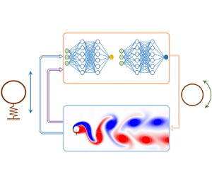
In the DRL framework, effective control strategies are learned through interactions between the DRL agent and the VIV environment. In the beginning, the DRL interacts with the VIV environment through randomized actions. Through trial and error, it learns how to exert a certain action when the system is in a certain state. In the meantime, it learns how to predict the long-term reward with this state information. As shown in figure 3, the state of the environment is represented by sensory-motor cues, and the action is the rotary motion imposed on the cylinder. The reward defined in (2.7) is then evaluated and fed to the agent, providing a baseline with which the agent can learn how to evaluate the control performance, so as to encourage it to develop a better controller that achieves a higher reward.
A schematic diagram of the DRL loop used in the present study. The DRL agent adopts two independent neural networks for decision-making (‘actor’) and reward evaluation (‘critic’). In the VIV environment, the instantaneous vorticity field is shown, together with grey lines to identify vortex structures based on the  $\lambda _{ci}$ criterion (Zhou et al. Reference Zhou, Adrian, Balachandar and Kendall1999).

Two sets of artificial neural networks are used in the agent, generally named the ‘critic’ and ‘actor’ networks. As depicted in figure 3, both networks use the state as their input. On the output side, the ‘critic’ network estimates the long-term discounted reward, whereas the ‘actor’ network models the control strategy. The mathematical expression for the objective of the ‘critic’ network is
 \begin{equation} J_{critic} = \hat{E}_t(-\hat{A}_t^2), \end{equation}
where the advantage function  $\hat {A}_t = R_t-V_\varTheta (s_t)$ determines the gain between the real long-term performance $R_t = \sum _{t'>t}{\gamma ^{t'-t}r_{t'}}$ and that predicted by the ‘critic’ network $V_\varTheta$ for a given $s_t$. Herein, the parameter $\gamma$ is a discount factor close to unity, so the long-term reward is preferred. In contrast, the objective of the ‘actor’ network is
 \begin{equation} J_{actor} = \hat{E}_t[\mbox{min}(q_t(\varTheta)\hat{A}_t, \mbox{clip}(q_t(\varTheta), 1-\epsilon, 1+\epsilon)\hat{A}_t)], \end{equation}
where  $q_t(\varTheta ) = {\rm \pi}_{\varTheta }(a_t|s_t)/{\rm \pi} _{old}(a_t|s_t)$ is the ratio of the probability of the current policy ${\rm \pi} _\varTheta$ adopting action $a_t$ according to state $s_t$ to the probability of the previous policy ${\rm \pi} _{old}$. The clip term inside (2.9) indicates that $q_t(\varTheta )$ is constrained to an interval $[1-\epsilon, 1+\epsilon ]$, where $\epsilon$ is the clipping rate needed to avoid an excessively large policy update. By using this proximal policy optimization-based DRL framework, it is expected that the agent can learn effective control strategies through stochastic trial and error. More details on this framework can be found in our prior studies (Ren et al. Reference Ren, Rabault and Tang2021a,Reference Ren, Wang and Tangb). The hyperparameters used in this study are listed in table 2. The adaptive moment estimation optimizer (abbreviated as ‘Adam’) is used when updating the parameters of both neural networks, with relatively small learning rates being used to help the training converge more stably.
Hyperparameters used in the DRL during the training stage.

Like many other machine learning applications that generally involve an exploration–exploitation process, DRL-guided AFC can also be divided into a training stage and a deterministic control stage. At the beginning of the training stage, the parameters of both neural networks are randomly initialized. During the training, the CFD simulation of each episode lasts for  $100T_0$, longer than $18$ vortex shedding periods of the uncontrolled case. An episode is a complete run with a reinitialized flow environment using a fully developed flow field and a control strategy updated according to the state-action–reward chain obtained in the last run. In each episode, states are extracted $10$ times within one $T_0$, and the actions are also enforced at the same pace. Furthermore, to enlarge the search space, actions are sampled from the bias-free Beta distribution (Chou et al. Reference Chou, Maturana and Scherer2017).
After the training reaches convergence, the deterministic control is performed, where the neural networks stop updating and only the ‘actor’ network is utilized to determine the action(s) with the given state data. Moreover, each action is no longer sampled from the aforementioned probabilistic distribution but is directly assigned its mathematical expectation to avoid randomness. To reach good convergence, the deterministic control lasts for  $200T_0$, and more actuations (100 times within one $T_0$) are sampled to perform smoother actuations.
3. Results and discussion
3.1. Interpretable learning with different state information
In a control system, the choice of sensors usually plays a crucial role. It is thus essential to determine the impact of each sensor as well as their combinations, so as to identify the most influential sensors. First, we explore the effects of different combinations of kinematic variables that provide feedback signals. Using the same hyperparameters listed in table 2 but different random seeds, we performed six groups of trainings and plotted the learning curves in figure 4, where the Reynolds number is all fixed as  $100$. Here $\langle {\cdot } \rangle$ indicates an average over one episode. Because the training process involves a certain level of randomness, we conducted three trials for each training in figures 4(a) and 4(b) and observed quite similar learning trends. For the cases in figure 4(c) that will be the focus of the remaining sections, we performed five trials. Therefore, figure 4 consists of $23$ training trials, i.e. 46 000 individual CFD cases in total.
Training processes using all six types of combinations of sensory-motor cues as the state space. In each training process, three or five independent trials are performed. The associated performances are shown with translucent lines, while the mean data are shown as thick solid lines.

In most trials, the learning starts with a rapidly decreasing trend and then proceeds with a gradually converging trend. All the learning curves eventually reach good convergence. Taking figure 4(c) as an example, the DRL reaches a level of  $\langle |y^*|\rangle \approx 0.01$ roughly at the $500$th episode, then progresses rather slowly beyond this point. Although the learning curve sometimes appears to show a non-decreasing trend, the agent can always escape from the locally optimal strategy and find the right search direction again after some unsuccessful trials. This fact reflects the self-adaptivity and reliability of the DRL agent in exploring nonlinear systems.
By comparing the learning curves of different combinations of sensors, it can be observed that using the velocity sensor alone leads to the worst control performance, while the combination of all three kinematic variables as sensors provides the best-converged strategy, where  $\langle |y^*|\rangle$ eventually reaches a level of approximately $0.002$, which is a remarkable level of VIV suppression. In addition, the $\ddot {y}^*$ sensor alone can lead to a VIV suppression to approximately $0.01$, yielding a less effective but simpler alternative for the control.
One question that comes to mind is how the DRL agent searches the optimal strategy in one single training. In other words, how does the AI agent think and make decisions during the exploration process? To answer these questions, we select four representative training trials with different state spaces from figure 4 and plot the scatters of the mean drag, vortex lift fluctuation and cross-flow displacement against the AFC forcing strength in figure 5. Although, as we have mentioned, the search path involves a certain level of randomness, it is surprising to see that figure 5 reveals some clear search paths. In particular, by comparing the search paths of  $\langle |y^*|\rangle$ in figure 5(a iii), one can observe that the training process can be roughly divided into three stages. In Stage I, the DRL agent explores a strategy that applies larger and larger forcing strength, which does gradually improve the control performance before hitting a plateau at approximately the $150$th episode, when $\langle |y^*|\rangle$ becomes close to $0.08$, with the fluctuation of $\omega ^*$ approaching its saturated value as can be more clearly observed in figure 7(b). In Stage II, a sudden turn appears in the $\langle |C_D|\rangle \sim \langle \omega ^{*2}\rangle ^{1/2}$ trajectory as well as the $\langle |y^*|\rangle \sim \langle \omega ^{*2}\rangle ^{1/2}$ trajectory, occurring roughly at the 150th–200th episode. Unlike in Stage I, although the forcing strength in Stage II gradually decreases, the control performance keeps improving, and reaches a level of $\langle |y^*|\rangle \approx 0.01$ at the end of Stage II around the $1000$th episode. The subsequent Stage III experiences a slower converging stage, in which the DRL agent carefully adjusts its strategy. Eventually, the DRL agent achieves a strategy that almost completely suppresses the VIV. The $\langle C_D \rangle \sim \langle \omega ^{*2}\rangle ^{1/2}$ curve shows a similar trend to that of the $\langle |y^*|\rangle \sim \langle \omega ^{*2}\rangle ^{1/2}$ curve, and the close relationship between $\langle C_D \rangle$ and $\langle |y^*|\rangle$ is further confirmed by figure 6(a). As the main hydrodynamic source that drives the VIV, the root-mean-square (r.m.s.) of the fluctuation part of $C_V$, i.e. $C_V'$, shows a gradually decreasing trend, except for scatter at the very beginning. From the trajectories in figure 5(a), one can see that the DRL agent adopts different strategies in the exploration process, and the fact that changing tactics when proceeding along one direction can no longer improve the performance implies that the decision making of the DRL agent is adaptive.
Trajectories of the (a) mean drag, (b) r.m.s. of the vortex force and (c) absolute value of the transverse displacement against the AFC forcing strength during training. Four training processes with different combinations of sensory-motor cues are shown in (a–a). The scattered points are coloured with the episode number, ranging from  $1$ to $2000$. Five representative cases in subpanels of (a) are marked with white star.

The trajectories of (a) the mean drag versus the absolute value of the transverse displacement and (b) the momentum coefficient versus power coefficient. Training with the full state space  $\{\ddot {y}^*, \dot {y}^*, y^*\}$ is used in this case.

However, one can only find a similar Stage I in figure 5(b iii) and in the first two stages in figure 5(d iii). In contrast, figure 5(c iii) only shows a gradually decreasing trend and eventually reaches a high level of vibration displacement, while exerting increasing AFC forcing and causing increased drag. Recalling figure 4(a), this case is actually a failure. The trajectories illustrated in figure 5 reflect that properly selected sensors play a crucial role in DRL-guided AFC, and can lead to distinct exploration paths during training. Importantly, the revealing of distinct stages implies that while exploring the VIV environment, the DRL agent is smart and capable enough to make radical adjustments to its control strategy when the existing learned strategies cannot make further contributions, which we believe is related to the underlying physics of the system being controlled.
To better understand the physics behind the search path, we draw the  $\langle {C_D}\rangle \sim \langle {|y^*|}\rangle$ curve and the $\langle {C_\mu }\rangle \sim \langle {C_P}\rangle$ curve in figure 6. The nearly monotonic variation of $\langle {C_D}\rangle$ against $\langle {|y^*|}\rangle$ implies that the reduction in the mean drag of the controlled cylinder is mainly accompanied by the reduction in the distance swept by the VIV cylinder. This close connection also suggests that $C_D$ could potentially be a good indicator of VIV control. In other words, in future applications, the drag and lift forces exerted on the cylinder could be good alternatives to provide feedback control signals. Figure 6(b) shows the connection between the kinetic energy of the rotary cylinder and the power supplied to the actuator. It is quite surprising to see that the three stages identified in figure 6 are the three edges of a triangle-like closed loop. That is, the initial $\langle {C_\mu }\rangle \sim \langle {C_P}\rangle$ pair roughly overlaps that in the final stage. To unveil more insights, a comparison will be made in § 3.3 between the initial control strategy (taking the 25th episode as a representative) and the final control strategy (the 1996th episode), which consume similar amounts of energy. It is also noted that Stage II proceeds along an energy-saving direction. However, throughout Stage III, $C_\mu$ is almost fixed while the energy supplied to the actuator monotonically increases. Eventually, the performance is further improved at the cost of an almost doubled energy input.
During the exploration process, since the actuation is sampled from a probabilistic distribution determined by the DRL agent, the recorded actuation and state both involve a certain degree of noise. To remove this impact, we utilize the control strategies learned from the  $5$th to the $1995$th episode ( $ep$ is the episode number), and perform deterministic runs every five episodes. In the second half of theses deterministic runs, the mean value, the fluctuation amplitude and the frequency of actuation are obtained, as depicted in figure 7(a–c). In figure 7(c), because the fast Fourier transformation is performed using the second half of each episode that involves $100T_0$, i.e. 10 000 actuation samples, the finest frequency resolution is $0.01$. This is why the action frequency appears discontinuous. From the case validations illustrated in Appendix A, we show that the actuation frequency follows exactly the same frequency as the kinematic variables, which is consistent with the overlapping frequency of $\omega ^*$ and $y^*$. We also calculate the phase lag between the actuation and the kinematic variables based on correlation analysis and present the results in figure 7(d).
The variations of the control quantities during a deterministic run from the fifth episode to the  $2000$th episode with an interval of five episodes. The (a) mean actuation, (b) fluctuation amplitude of actuation, (c) frequency of actuation and (d) phase lag between the actuation and kinematic variables. The three stages are identified again and classified using different background colours.

From figure 7, one can deduce the following features of the three stages. In Stage I ( $ep < 150$), the DRL agent adjusts both the amplitude and frequency of the AFC forcing, both being increased. In Stage II ( $150 < ep < 1000$), the DRL agent also adjusts both the amplitude and frequency of the AFC forcing, both being gradually reduced though. In Stage III ( $ep > 1000$), the DRL agent gradually adjusts its phase lag against the kinematic variables. A phase lag close to $20^\circ$ between $\omega ^*$ and $\ddot {y}^*$ is finally obtained. In both Stages I and II, action biases, i.e. non-zero mean actions, are observed. It takes a long trial process for the bias to disappear at the end of Stage II. This problem almost vanishes in Stage III.
In the above divisions into three stages, the transition boundary from Stage I and Stage II is quite clear based on either the peak of the action amplitude or the location of the largest action frequency. However, because the change from Stage II to Stage III is relatively vague, in figure 7, the boundary between Stage II and Stage III is only a rough approximation; from the aspect of energy utilization shown in figure 6(b), where  $C_\mu$ reaches its minimum and $C_P$ starts to increases again. It also remains a question why Stage I transits to Stage II, which is not simply a consequence of saturated action. This question will be discussed in § 3.3.
It is observed from figure 7(d) that the phase between  $\omega ^*$ and $\ddot {y}^*$ is the closest, suggesting that $\ddot {y}^*$ always reacts with changes in $\omega ^*$ faster than the other two sensors. We guess this is a key reason why the $\ddot {y}^*$ sensor is selected from the very beginning, and plays a key role during the whole exploration process.
Note that the above interpretations of the learned control strategy are essentially different from the cluster method (Fernex et al. Reference Fernex, Noack and Semaan2021; Li et al. Reference Li, Fernex, Semaan, Tan, Morzyński and Noack2021), where the state information is projected onto a low-dimensional phase space and different strategies are then clustered. By contrast, the way we interpret the search path is less general but more straightforward from the physics perspective, and benefits from a small number of sensors. In addition, the effect of hyperparameters used in the DRL is examined and the data are shown in Appendix B, where it is indicated that the above findings are less sensitive to the hyperparameters. The fact that different hyperparameters lead to the very similar division of three stages confirm that the above findings are reasonable and solid.
3.2. Sensitivity analysis
For control with three sensor signals, it is worthwhile to know how sensitive each sensor is in the control strategy. Therefore, we perform a sensitivity analysis via the Sobol method (Saltelli Reference Saltelli2002; Sobol Reference Sobol2014), based on SALib – a sensitivity analysis library implemented in Python. Here the ‘actor’ network that establishes the mapping between sensor signals and the control action is utilized, together with randomly selected values within the actuation range. Total sensitivity indices  $S_T$ are used to quantify the sensitivity of each control input to the control output. According to the definition in Sobol (Reference Sobol2014), $S_T$ is an invariance-based sensitivity index that measures the contribution of the variance of each input argument to the variance of the output, which including all variance caused by its interactions, of any order, with any other input variables. In a whole training, $S_T$ of each sensory-motor cue is shown in figure 8, where, the same as in the deterministic runs, we perform the sensitivity analysis from the $5$th to $2000$th episode with an interval of five episodes.
The total sensitivity index for all sensory-motor cues during one training. The sensitivity analysis is conducted from the fifth to the  $2000$th episode with an interval of five episodes.

First, it is seen that the  $\ddot {y}^*$ sensor maintains a much higher sensitivity level than the other two sensors. This qualitative conclusion is consistent with results in figure 4, where the $\ddot {y}^*$ sensor is the most effective one. Second, the evolution of $S_T$ also exhibits similar features to the three stages identified in § 3.2. As revealed in figure 7, the DRL agent adjusts the actuation amplitude and frequency during Stages I and II, where theoretically one signal among the three kinematic variables is enough. This is why $S_T$ of $\ddot {y}^*$ shows an increasing trend during these two stages. However, because Stage III is a phase-adjusting stage and the $\ddot {y}^*$ sensor alone cannot achieve this, the contributions of the other two sensors start to grow during this stage. This explains why the $S_T$ of both $y^*$ and $\dot {y}^*$ show a dramatically increasing trend in Stage III. From the sensitivity analysis, one can also see that adjustments of the actuation amplitude and frequency are easier than the long-march phase adjustment process.
3.3. Deterministic control using strategies learned at different stages
After the DRL training reaches convergence, we obtain the control law established by the ‘actor’ network. Among the 23 training processes, we select a few cases with a full state space  $\{\ddot {y}^*, \dot {y}^*, y^*\}$ as representatives, occurring at the $25$th, the $150$th, the $200$th, the $998$th and the $1996$th episode. We conduct a group of deterministic controls using these strategies learned at different episodes to elucidate the difference of control performance.
Figure 9 demonstrates temporal variations of the rotary forcing recorded in episodes of different stages. From figure 9(e), one can see that the actuation reaches saturation in the early few control cycles, and then gradually becomes quasisteady. To maintain the control performance, a rotational velocity with an amplitude of approximately  $0.4$ is required, corresponding to the linear velocity at the edge of the cylinder being less than $U_0/5$. Note that the vortex shedding frequency does not deviate from the natural resonance frequency, as confirmed in Appendix A, suggesting that the main physical mechanism of VIV suppression lies in that the DRL-guided control successfully alters the flow field to an attenuated vortical flow, and that the lift generated by the vortices are balanced by the Magnus effect induced by the rotary forcing. Intriguingly, from all selected cases, as well as the information in figure 7(c), the DRL agent does not proceed with seeking a proper frequency being the vortex shedding frequency in the uncontrolled situation, or its super harmonics or subharmonics, so as to utilize the ‘lock-on’ effect, which is what the AFC community usually adopted.
(a) Temporal variations of the rotational velocity after the AFC is turned on. (b) The frequency spectrum of  $\omega ^*$ in the quasisteady state. Here $f^*$ denotes the frequency normalized by $T_0^{-1}$. The $25$th, $200$th and $1996$th episode are representatives of Stage I, Stage II and Stage III, respectively. The $150$th episode is the boundary between Stage I and Stage II and the $998$th episode the boundary between Stage II and Stage III.

One can now observe another significant fact that at Stage II, the DRL agent gradually learns the control strategy that a large forcing shall be exerted at the first few periods so as to rapidly mitigate the vibration to a new and low-amplitude state. After that, the periodic or quasisteady forcing is applied to fine tune this state. In this sense, the initial stage of each episode that involves a few vibration cycles with higher forcing strength actually plays a vital role in achieving the final VIV suppression objective. Without this initial process, the VIV control can hardly be realized even with a higher-level of forcing, just like cases in Stage I. This finding suggests that the DRL agent is really smart. This type of control strategy can hardly be done in the open-loop manner.
Temporal variations of quantities related to energy consumption, i.e.  $C_P$ and $C_\mu$, are depicted in figure 10. Under the converged control strategy at the $1996$th episode, after the initial stage, in which the DRL-guided control strategy requires a relatively large energy input to rapidly reduce the vibration, only a small amount of energy input is needed to maintain the control performance in the quasisteady state. In contrast, the $25$th episode does not show this kind of adaptation. Further quantitative comparisons are based on the power-saving ratio ( $PSR$), defined as
 \begin{equation} PSR = \frac{\langle \Delta P_D \rangle_{T}}{\langle P_C \rangle_{T}}, \end{equation}
where  ${\Delta P_D = -\Delta F_DU_0}$ denotes the saved power used to drive the streamwise motion in the situation where the cylinder is cruising with a speed of $U_0$. This quantity is averaged within a time horizon of one vortex shedding period. Here $P_C$ is the power consumed by the AFC. After normalization, we have $PSR = -\langle \Delta C_D \rangle _{T}/\langle {C_P}\rangle _{T}$, where $\Delta C_D$ is the reduced drag coefficient. Therefore, as estimated in the quasiperiodic state, the power saving ratio is $78.7$ if compared with the uncontrolled VIV case, and $1.85$ if compared with the uncontrolled stationary case. In some prior studies (Protas & Wesfreid Reference Protas and Wesfreid2002; Bergmann, Cordier & Brancher Reference Bergmann, Cordier and Brancher2005), where rotary control was used for drag reduction under laminar conditions, $PSR$ did not exceed $1.0$. Therefore, the DRL-guided control presented in this study is energetically efficient.
Temporal variations of the power coefficient and the momentum coefficient in the deterministic control using controllers learned in selected episodes.

Recalling that in figure 5(a i–iii), similar levels of rotary amplitude were found in the initial and final training stages, it is interesting to see how apparently similar actuations lead to distinct control results. To find the reason, we illustrate the temporal variations of  $\omega ^*$, $y^*$, $\dot {y}^*$ and $\ddot {y}^*$ during one quasisteady cycle of the $25$th and the $1996$th episodes in figure 11. Four instantaneous snapshots are selected, when $\ddot {y}^*$, $\omega ^*$, $\dot {y}^*$ and $y^*$ are, in sequence, at their lowest positions. Although a slightly biased $\omega ^*$ appears in the $25$th episode, the amplitudes of $\omega ^*$ in the two cases are very close, i.e. approximately $0.4$. It can be found that the forcing frequency of the $25$th episode is slightly higher than that of the well learned strategy in the $1996$th episode. Furthermore, the $\omega ^*-\ddot {y}^*$ phase lag in the $25$th episode is also slightly smaller, coinciding with the data in figure 7.
The temporal variation of the rotational forcing as well as the kinematic variables in the quasisteady state. Flow fields at four representative instants are demonstrated. The unsuccessful  $25$th episode is shown here for comparison purposes.

In figure 5, although the fluctuation amplitude of the rotary actuation in the two episodes do not show big differences, the two strategies do lead to distinct FSI dynamics. With the control strategy learned in the  $25$th episode, the wake exhibits a C(2S) vortex shedding pattern (Williamson & Roshko Reference Williamson and Roshko1988) like in the uncontrolled case, where two single vortices shed within one vibration cycle, and the like-signed vortices coalesce in the downstream region, which is approximately $15$ diameters from the cylinder. On the contrary, a transition to the 2S pattern is observed in figure 11(b). As seen in the VIV phase diagram provided by Williamson & Govardhan (Reference Williamson and Govardhan2004), the 2S pattern is usually associated with a larger wavelength, or smaller vortex shedding frequencies, and this is confirmed by the above results. Intuitively, the near-wall shear layer in figure 11(a) forms an inclined angle using the $25$th episode strategy, which is measured between the centreline of the wake and the boundary of the positive and negative shear layers. This phenomenon appears to be almost symmetrical in figure 11(b). This flow feature also reveals well-controlled structure vibrations.
From instant E to instant F, the negative rotational velocity (clockwise direction) transports momentum from the upper right-hand side of the wake to the lower right-hand side, mitigating the asymmetrical force induced by the near-wall flow structures. In this sense, maintaining the relatively good stability of the upper and lower shear layers is vital for the success of the present DRL-guided VIV control. Now, one can also imagine that if the rotary actuation is performed somewhat earlier (corresponding to a smaller  $\omega ^*-\ddot {y}^*$ phase lag) or later (corresponding to a larger $\omega ^*-\ddot {y}^*$ phase lag), the influence of shear layers on the lift could become quite different. Evidence in the later § 3.4 would confirm that the DRL agent does remarkably enhance the stability of this FSI system.
3.4. Deterministic control using the converged control strategy
With the control strategy learned at the  $1996$th episode, we illustrate in figure 12 the three-dimensional (3-D) trajectory of $\ddot {y}^*\unicode{x2013}\dot {y}^*-y^*$, with and without the control. In this 3-D space, the uncontrolled trajectory forms a periodic orbit. With a phase lag of $180^\circ$ between $\ddot {y}^*$ and $y^*$, the projection on the two-dimensional (2-D) $\ddot {y}^*\unicode{x2013}y^*$ plane appears to be roughly a straight line. After the control is turned on, this orbit gradually shrinks to its centre and finally reaches the quasiequilibrium state, a tiny closed loop in 3-D space.
The 3-D scatters of  $\ddot {y}^*-\dot {y}^*-y^*$, with projections on the 2-D planes. The scatters are denoted by blue square cubes and pink spheres, respectively, for instants before and after the control is turned on.

Temporal variations of the hydrodynamic force and torque coefficients, as well as the vibration response, are depicted in figure 13. Less than five VIV periods, after the DRL agent starts to mediate the originally periodic FSI system, the FSI system falls into a quasisteady state. In this controlled state, the drag exerted on the cylinder is reduced by  $37\,\%$ compared with the uncontrolled VIV case, accompanied by a reduced drag fluctuation of $98\,\%$. Furthermore, the quasisteady drag resembles that in the uncontrolled stationary case. Therefore, the drag reduction mainly stems from the narrowed distance swept by the cylinder, as shown in figure 13(d). In figure 13(b), the lift experiences a sharp change at the beginning of the control, even exceeding that of the uncontrolled VIV case in the first vortex shedding period, then decays quickly as the control continues and is eventually suppressed to almost zero. Meanwhile, a large torque with sharp variations in the beginning is required to drive the rotary motion, as can be seen in figure 13(c). Figure 13(d) demonstrates the successfully suppressed VIV, where the final vibration amplitude is only approximately $0.2\,\%$ of the cylinder diameter (an enlarged view can be found in figure 11), corresponding to a VIV amplitude suppression rate of $99.6\,\%$. Furthermore, for the VIV case, only a $1.3\,\%$ frequency shift is observed after control. This almost unaffected VIV frequency indicates that the system is still in the locked-in condition.
Time histories of (a) the drag coefficient  $C_D$, (b) the lift coefficient $C_L$, (c) the moment coefficient $C_M$ and (d) the transverse displacement $y^*$. The uncontrolled stationary case, the uncontrolled VIV case, and the DRL-controlled case are organized together for comparison purposes.

Comparisons of the three lift force components are depicted in figure 14, where  $C_E$ is reduced by a factor of five for the sake of clarity. From the definitions in § 2.1, one can see that the vortex force is the hydrodynamic source that drives the VIV. The non-harmonic variation of $C_V$ stems from the vortex shedding mode. After control, the fluctuation of $C_V$ is reduced by a factor of over $700$. This can be viewed as further evidence of well-suppressed VIV. It is noted that the mean $C_V$ is not zero, which is a consequence of the non-zero mean actuation, as evidenced by the fast Fourier transformation results in figure 9(b).
Temporal variations of the three lift components of (a) the uncontrolled VIV case and (b) the DRL-controlled VIV case (the vortex force, the added-mass force and the elastic force).

In order to figure out why the VIV can be suppressed in the  $1996$th episode, the lift variation in one cycle is shown in figure 15 as well as three instants corresponding to minimum, moderate and maximum lift force, respectively. The pressure field near the cylinder and the vorticity field are also depicted. For the three cases, the vortices that form and shed from the cylinder surface play key roles in lift generation and the resulting VIV.
Temporal variation of lift coefficient. Pressure field and vorticity field at three representative instants are demonstrated. For the DRL-controlled VIV case, arrows are shown to represent the corresponding rotary direction and amplitude, wherein a full circle means  $|\omega ^*|=0.4$.

In the uncontrolled stationary case, when  $C_L$ is at its minimum at instant A, the anticlockwise vortex (labelled as ‘acw-vortex’) at its lower surface is forming and the clockwise vortex (labelled as ‘cw-vortex’) is about to shed from the upper surface. Correspondingly, the pressure on its lower surface is much lower than that on the upper surface, resulting in a negative lift force. At instant B, both the acw-vortex and cw-vortex have moved to the downstream. The positive and negative shear layers lead to a balanced pressure distribution on the cylinder.
In the uncontrolled VIV case, at instant D, the cylinder is moving downwards and is near its lowest position. The cw-vortex is about to shed and has a lesser effect on the cylinder. The negative shear layer on the upper surface provides larger pressure than the positive shear layer on the lower surface, resulting in the maximum negative lift. At instant E, the cylinder is near its equilibrium position and is moving upwards with almost its largest transverse velocity. The upward motion creates a high-pressure region on the upper left-hand surface, meanwhile the cw-vortex provides a low-pressure region on the upper right-hand surface, leading to a balanced transverse force.
In the DRL-controlled VIV case, the well-controlled cylinder is nearly stationary. At instant G, since the cylinder is rotating in the anticlockwise direction (i.e. positive  $\omega ^*$), the shedding of an acw-vortex is promoted earlier (compared with the uncontrolled stationary case), thus exerting little effect on the pressure distribution over the cylinder surface. The lift force is thus suppressed to a value around zero. Similarly, at instant I, the early shedding of a cw-vortex is induced by the clockwise rotation of the cylinder.
The above results reveal that the DRL knows when to exert the right amount of rotary forcing, so that effective control can be conducted by actively adjusting the phase lag between the rotational forcing and the lift (or the transverse displacement).
To reveal control in a transient process, we present the time histories of the cross-flow displacement  $y^*$, the rotational velocity $\omega ^*$ and the rotational acceleration ${\rm d}\omega ^*/{\rm d}t^*$* in figure 16, as well as the pressure and vorticity fields at the selected instants figure 16(a) to figure 16(i). The dark and light grey background marks three cycles, all starting from a zero $y^*$ with upwards motion. The instant in figure 16(a) is the starting point. The control starts at figure 16(a). At instants in figure 16(a,d,f) and figure 16(h), sharp changes of the control forcing occur, whereas at instants in figure 16(c,e,g) and figure 16(i), the oscillation displacement reaches its local maximum or minimum. In these cycles, the control forcing maintains mostly at its maximum allowed value, either positive or negative.
Temporal variation of the cross-flow displacement  $y^*$, the rotational velocity $\omega ^*$ and its temporal derivative ${\rm d}\omega ^*/{\rm d}t^*$. Pressure field and vorticity field at representative instants are demonstrated.

It is observed that the sign of  $\omega ^*$ is always opposite to that for $y^*$, suggesting that the DRL agent adopts a simple yet effective opposition control in this initial stage, by utilizing the Magnus effect, i.e. the anticlockwise rotary motion induces a downward force, and vice versa. Therefore, the force induced by rotary motion would counteract the recovery elastic force. As revealed in figure 14, the elastic force is much larger than the lift components. As such, the rotary induced lift force can mitigate the very large recovery elastic force, gradually slowing down the cylinder's transverse motion.
Note that the Magnus effect is only one of the lift components. Another lift component induced by the vortex formation and shedding is nonlinear and complex. The phase difference between the vortex shedding and the cylinder rotation can affect this lift component, which is reflected by the clear phase lags between  $y^*$ and $\omega ^*$, at instants in figure 16(b,f). As having been discussed in § 3.1, this type of phase difference also appears in the quasisteady stage, suggesting that the DRL agent has learned a more complicated strategy than the opposition control.
From instant in figure 16(a) to figure 16(b),  $\omega ^*$ rapidly increases, which retards the growth of the cw-vortex. At the instant in figure 16(b), $\omega ^*$ reaches its local maximum and then sharply decreases, promoting for the shedding of the cw-vortex and the formation of the following positive shear layer as evidenced at the instant in figure 16(c). Similar phenomena can also be found at instants in figure 16(d,f,h). Comparing instants in figure 16(b,d,f,h), the large low-pressure region gradually becomes smaller and the pressure difference between the upper and lower surfaces is gradually attenuated. This indicates that the DRL-guided control successfully modulates the vortex dynamics. At the instant in figure 16(c), the elastic force is at its negative maximum, the clockwise rotation stimulates the growth of the negative shear layer while retarding the growth of the positive shear layer, leading to an upwards lift force so as to counteract downward elastic force. Similar phenomena can be found at instants in figure 16(e,g,i).
The time-averaged flow fields displayed in figure 17 further reveal the impact of DRL-guided control. Through comparisons, one can note that the low-velocity far downstream region in the uncontrolled VIV case vanishes after control, making the DRL-controlled flow resemble the uncontrolled stationary case, while the length of the recirculation bubble represented by the zero streamwise velocity contour is increased by  $16\,\%$. Prior studies (Rabault et al. Reference Rabault, Kuchta, Jensen, Réglade and Cerardi2019; Ren et al. Reference Ren, Rabault and Tang2021a) have shown that the change in the drag force is strongly related to the length of the recirculation bubble, where an elongated recirculation bubble is usually accompanied by attenuated and delayed vortex shedding. Furthermore, the attenuated transverse flow after control indicates a much weaker source of cross-flow vibration.
Comparisons of the time-averaged streamwise velocity, transverse velocity and pressure field between (a) the uncontrolled stationary cylinder, (b) the uncontrolled VIV cylinder and (c) the DRL-controlled VIV cylinder. In subpanels (a i) and (c i), the recirculation bubble is represented by the  $\bar {u} = 0$ contour line.

3.5. Dynamic mode decomposition analysis
To demonstrate changes in the coherent flow structures and flow stability characteristics before and after control, we perform a series of DMD analyses over three flow types, i.e. the uncontrolled stationary case, the uncontrolled VIV case and the DRL-controlled case. Compared with the more popular method of proper orthogonal decomposition, which extracts flow structures based on their energy ranking, DMD provides more clear information related to time or frequencies. With DMD, the unsteady flow field can be reconstructed using limited DMD modes, i.e.
 \begin{equation} \boldsymbol{v}(\boldsymbol{x}, t) = \sum_{i=0}^{L\leqslant N}{\rm e}^{\mu_it}\boldsymbol{\varPhi}_i(\boldsymbol{x}), \end{equation}
where  $N$ is the total number of snapshots. The real and imaginary parts of $\mu _i$ represent the growth rate and angular frequency of the $i$th DMD mode $\boldsymbol {\varPhi }_i(\boldsymbol {x})$, respectively. Note that we have included in $\boldsymbol {\varPhi }_i(\boldsymbol {x})$ the corresponding amplitude, which reflects the influence of the initial data on the DMD mode. Detailed information about the DMD algorithm can be found in Schmid (Reference Schmid2010) and Wang et al. (Reference Wang, Tang, Yu and Duan2017a).
In this study, we extract a series of flow fields with a time interval of  $0.02T_0$ within a duration of one vortex shedding period, and the numbers of snapshots used in the three flow systems are $307$, $275$ and $279$, respectively. In our tests, these numbers of snapshots are sufficient to obtain converged DMD results. When conducting the DMD analysis, we select part of the whole domain ranging from $x^* = 0.50$ to $x^* = 14$ and from $y^* = -4$ to $y^* = 4$. It should be noted that the zone that contains the moving cylinder is removed, so as to avoid the effect of moving structure on the DMD analysis. As can be seen from the DMD modes of figure 19, this subdomain is large enough to cover most flow features both around the cylinder and in the wake.
Sorting the DMD modes by their frequencies, we obtain the frequencies (non-dimensionalized as Strouhal numbers) and growth rates of all DMD modes. For the sake of brevity, we list the data for the first four DMD modes in table 3. Here, the Strouhal number of Mode 1 is consistent with the lift frequency extracted in figure 13, and is the dominating fluctuation frequency, i.e. the vortex shedding frequency. The frequencies of Mode 3 and Mode 5 correspond to two and three times the vortex shedding frequency, respectively. The first four growth rates for all three cases are of an order of  $10^{-4}$ or smaller, implying that the corresponding modes are neutrally stable.
Comparisons of the amplitude, Strouhal number and growth rate of the first four DMD modes.

In addition to table 3, we plot the growth rate against the Strouhal number for all DMD modes in figure 18. The negative-frequency points are the adjoint modes, making the data symmetrical along the vertical axis. For the uncontrolled stationary case, only a few modes including Mode 1 have positive growth rates. For the uncontrolled VIV case, approximately one-third of the DMD modes have positive growth rates. However, after control, no positive growth rate is found, proving that the DRL-guided control does enhance the flow stability. Moreover, the two peaks in the uncontrolled case suggest that the flow instability can be triggered by either low-frequency or high-frequency perturbations. This potential source of instability is eliminated by the DRL-guided control.
Scatter plots of the Strouhal number versus growth rate. (a–c) Results for the uncontrolled stationary case, the uncontrolled VIV case and the DRL-controlled VIV case, respectively. (d) A comparison between the three cases involving only the low-frequency modes. The colours determine the mode number. Negative Strouhal numbers represent the corresponding adjoint modes.

Figure 19 shows the dominant DMD modes of the uncontrolled stationary case, the uncontrolled VIV case and the DRL-controlled VIV case. Among these modes, Mode 0 is the mean mode that corresponds to the time-averaged vorticity field, where one can see a pair of symmetrical shear layers. After control, Mode 1 shows a much narrower shear layer compared with figure 19(b i), as well as an elongated shear layer compared with figure 19(a i), consistent with the time-averaged variables illustrated in figure 17. Mode 1 is connected to the lift fluctuation and is thus strongly associated with VIV suppression. In Mode 1, one can see in-line alternating vortices behind the cylinder in figure 19(a ii) and figure 19(c ii), which are much narrower and weaker than those in the uncontrolled VIV case. Vortices whose centre are off the centrelines appear in the uncontrolled VIV case, suggesting that their momentum along the cross-flow direction is larger, gained when interacting with the cylinder. This phenomenon is evidence of larger lift fluctuations of the cylinder exerted by the surrounding fluid. These flow features explain the changes after the VIV is suppressed. In Mode 3, one can see pairs of counter-rotating vortices whose centres are symmetrical along the centreline of the wake flow, which is the main cause of drag fluctuation. Comparing figures 19(b iii) and 19(c iii), the attenuated near-wall flow structures after control explain the remarkably mitigated drag fluctuation.
The three dominant DMD modes calculated from the uncontrolled stationary case, the uncontrolled VIV case and the DRL-controlled VIV case.

Therefore, the DMD analysis explains the remarkable enhancement of flow stability achieved with DRL-guided control. Furthermore, changes in the coherent structures show that DRL-guided control mediates the flow to a state resembling that of the stationary case while generating an elongated recirculation bubble as well as weak small-scale flow structures.
3.6. Robustness at different Reynolds numbers
In this section, we test the robustness of the DRL-guided control strategy within a Reynolds number range of  $[40, 300]$. Instead of directly applying the learned strategy to the off-design conditions, we introduce the idea of transfer learning to further improve performance. We retain almost all of the same set-ups as in the $Re = 100$ case but reinitialize the ‘actor’ and ‘critic’ neural networks with well-trained model parameters as in the control strategy of § 3.2. The training then continues until reaching convergence. The converging trends for various Reynolds numbers are shown in figure 20. Note that in figure 20(a), the actuation range of $\omega ^* \in [-1, 1]$ is retained. However, due to the saturated forcing occurring around $Re = 180$, we enlarge the actuation range and choose an interval of $[-2, 2]$ for the $Re = 200$ case. For the $Re = 300$ case, we choose a larger actuation interval of $[-3, 3]$ and start the transfer learning via inheriting the strategy learned at $Re = 200$. Instantaneous vorticity fields, as well as the vibration responses and AFC forcing at selected Reynolds numbers, are organized into figure 21.
Transfer learning for cases at Reynolds numbers ranging from  $40$ to $300$. In panels (a,b), the first episode starts from the learned strategy at $Re = 100$. For the $Re = 300$ case in (b), the DRL agent inherits the converged strategy from the $Re = 200$ condition.

The flow fields, vibration response and rotational forcing from DRL-guided control at selected Reynolds numbers. Instantaneous snapshots of (a) the uncontrolled VIV case and (b) the DRL-controlled VIV case. (c) Temporal variations of the vibration amplitude before and after the control is turned on, as well as the AFC forcing. In panels (a,b), instants are selected when the cylinder is crossing its equilibrium position with upward velocity.

At  $Re = 40$, the VIV is under the subcritical Re condition (Mittal & Singh Reference Mittal and Singh2005). When the DRL-guided control is turned on at $t^* = 0$, the flow becomes steady and only slight rotary forcing is needed to sustain the suppressed VIV. For $Re \leqslant 120$, the starting point of the transfer learning shows that the learned strategy at $Re = 100$ is already good, capable of suppressing the VIV to a level around $0.001$ times the cylinder diameter. In the following transfer learning process, the curve only shows a very slow decreasing trend, indicating that there is almost no more space for the DRL agent to improve its performance. As Re is further increased to $140$, a larger VIV amplitude is noted in the beginning, suggesting that the learned strategy cannot be directly applied under this condition. However, with transfer learning, the control performance can be further improved to a level of roughly $\langle |y^*|\rangle = 0.003$. This case vigorously verifies the advantage of transfer learning.
As Re is further increased to  $160$, a similar trend is observed as in the case of $Re = 140$, while showing a higher starting point and less effective control performance. This change suggests that the increased Re starts to make the VIV control more difficult. The DRL-guided control experiences a failure when Re is increased to $180$, and the performance is only slightly improved as the learning proceeds. The finally converged strategy shows unsuccessful VIV suppression, as depicted in figure 21(c iv). Meanwhile, we also note that the actuators have already reached saturation at this point, explaining why the DRL can hardly improve the performance during transfer learning. Therefore, we expand the actuation range in cases when a higher Reynolds number is involved.
From the perspective of the flow field, one can also observe that in figure 21(a ii,iii,b ii,iii,c ii,iii), a transition from the C(2S) vortex shedding pattern to the 2S pattern occurs. The phenomenon that the DRL-controlled flow field shows a larger centre-to-centre distance between two adjacent and like-signed vortices suggests that the vortex shedding period is enlarged by the rotary control. The less successful case, the  $Re = 180$ case, does not show a pattern transition but the distance between the parallel-moving vortices is narrowed. At $Re = 200$ and $Re = 300$, a dramatic transition of the alternating 2S vortex shedding pattern to the C(2S) pattern is observed, which can be explained by the high-frequency rotary forcing in figures 21(c v) and 21(c vi). This frequency shift in the rotary forcing reveals a distinct mechanism of VIV control, which, as concluded by Du & Sun (Reference Du and Sun2015), is due to the fact that the vortex shedding frequency is attracted to the forcing frequency. In other words, for the cases when $Re = 200$ and $Re = 300$, the control strategy discovered by the DRL actually utilizes the ‘lock-on’ effect. A similar vortex shedding pattern of the $Re = 300$ case can also be found in the work of Protas & Wesfreid (Reference Protas and Wesfreid2002), where harmonic rotary control with a frequency of two times the vortex shedding frequency was utilized. In fact, this frequency ratio matches the forcing frequency over the vibration frequency in figure 21(c vi) well.
It should be noted that in this section, while performing the transfer learning, we do not follow the prior practice in § 3.1, in which a group of three or five trials was conducted so as to avoid the possible effects of training randomness, and thus we do not intend to imply that the strategies showcased in figure 21 are the only optimal ones. Our main objective is to demonstrate the robustness of DRL-guided control in terms of different Re, and these cases indeed prove that the DRL-guided control is qualified. In addition, we understand that the VIV at  $Re=300$ involves the 3-D effect. Here we still choose the 2-D simulations so as to keep consistent with the other cases. In the future, 3-D and even the fully turbulent conditions would be thoroughly studied. Note that in higher-Reynolds-number conditions, our choice of state space, action and reward for VIV control would not be affected, thus we anticipate that the model-free and data-driven DRL could possibly be still effective.
3.7. Robustness with a perturbed upstream flow
In the Introduction, we mentioned that current studies related to DRL-guided AFC lacks sufficient tests and confirmations with perturbed environments, which is the more realistic situation. In this section, we further verify the robustness of the DRL-guided control strategy in a perturbed upstream flow. We superpose a harmonic perturbation to the uniform velocity  $U_0$ at the inlet (Konstantinidis & Bouris Reference Konstantinidis and Bouris2009; Zhao et al. Reference Zhao, Kaja, Xiang and Yan2013; Ma et al. Reference Ma, Zhou, Wang, Yang, Li and Cao2021), and thus the inlet velocity becomes
 \begin{equation} U_0' = U_0(1+\epsilon_{p}\sin(2{\rm \pi}f_pt)), \end{equation}
where  $\epsilon _p$ is the perturbation amplitude and $f_p$ the perturbation frequency. In the study of Konstantinidis & Bouris (Reference Konstantinidis and Bouris2009), both the harmonic (as (3.3)) and the non-harmonic upstream perturbations induced complicated flow patterns and hydrodynamic force responses. In a recent study that focused on the effect of a sinusoidal streamwise gust on the vortex-induced force on an oscillating rectangular cylinder using both wind tunnel experiments and a CFD approach (Ma et al. Reference Ma, Zhou, Wang, Yang, Li and Cao2021), it was found that the flow structure was sensitive to the upstream flow condition. For demonstration purposes, we fix the perturbation amplitude to quite a challenging level, $\epsilon _p = 0.5$ (a value of $0.325$ is used in Konstantinidis & Bouris (Reference Konstantinidis and Bouris2009) and Zhao et al. (Reference Zhao, Kaja, Xiang and Yan2013)). In this sense, the robustness is essentially different from that of § 3.4, due to the fact that the Reynolds number of the incoming velocity dynamically varies within a range of $[50, 150]$. We then focus on the effect of perturbation frequency on the DRL-guided control and test a series of $f_p$, with the dimensionless frequencies $f_pT_0$ being $1$,
$1$,  $0.5$, $0.25$ and $0.125$, respectively. For consistency, the DRL-guided control uses the same learned strategy that was tested in §§ 3.2 and 3.3. The instantaneous snapshots, as well as the temporal response of the vibration amplitude and the AFC forcing, are depicted in figure 22.
Comparisons of the instantaneous streamwise velocity between (a) the uncontrolled cases and (b) the DRL-controlled cases. (c) The vibration responses and rotational forcing both before and after the AFC is turned on. Cases with four perturbation frequencies are illustrated from subpanel (i) to subpanel (iv).

In cases where the perturbation frequency is large, the streamwise velocity is easier to mix up, causing a less clear streamwise wave as shown in figure 22(a). As shown by the distributions of the high-velocity and low-velocity regions, which can be regarded as signatures of the vibrating cylinder, low-frequency perturbations generally have a stronger impact on the flow field. After control, the DRL-controlled flow field appears to have well-attenuated flow signatures for all perturbation frequencies. Furthermore, as can be seen from figure 22(c), the vibrations are all well suppressed. After the dynamical vibration reaches convergence, the average  $\langle |y^*|\rangle$ become $0.0013$, $0.0027$, $0.0141$ and $0.0028$, respectively. In addition, when perturbations are introduced to the FSI system, one can see remarkable reactions from the variations in $\omega ^*$. In figure 22(c i), the rotary control is almost unaffected by the perturbation. However, in figure 22(c ii–iv), the AFC forcing almost reaches saturation. When the perturbation frequency approaches the VIV resonance frequency (see table 1), we see the most challenging case with $f_pT_0$ being $1/4$, as shown in figure 22(c iii). In this case, the asynchronous perturbation and vibration cause difficulties for the DRL in making decisions and induce high-frequency and saturated actuations.
The onset of complicated frequency features reflects the significant impact of the perturbed upstream flow on the flow and vibration response, whereas the DRL agent can still successfully realize the vibration suppression objective. Therefore, the above robustness tests prove that the DRL-guided control is not only efficient under uniform upstream flow conditions, but is also successful when the environment is experiencing a certain level of perturbation.
In our prior study (Ren et al. Reference Ren, Wang and Tang2021b) targeted at eliminating the wake signatures of a circular cylinder, it was observed that the attenuated wake signature is closely related to the hydrodynamic forces exerted on the cylinder, as well as the vibration characteristics. The findings here, on the opposite side, show that the suppression of vibration also facilitates the attenuation of wake signatures, even with strong upstream perturbations.
4. Summary and conclusion
In the present work, we have demonstrated the application of DRL-guided AFC to the classical VIV problem. Through self-rotary control guided by the DRL agent in a real-time and self-adaptive manner, the VIV was eventually suppressed, with a reduction in the VIV amplitude of  $99.6\,\%$. Through case studies and detailed analysis, we have drawn the following conclusions.
(i) Under the lock-in condition, the DRL-guided AFC was found to be capable of suppressing the VIV with relatively small actuations and energy input, indicating that the control method is effective and efficient.
(ii) With all possible combinations of sensory-motor cues being tested, the combination of displacement, velocity and acceleration sensors showed the best performance, while the acceleration sensor alone played the most significant individual role. This finding was confirmed by sensitivity analysis. Three distinct search paths during training were observed, intuitively illustrating the logical approach of the AI and showing that the DRL exploration process is interpretable.
(iii) The DMD analysis showed that the DRL control remarkably enhanced the flow stability and transformed the flow field into a state resembling an uncontrolled stationary one, while leading to an elongated recirculation bubble and mitigating small-scale flow structures. The DMD analysis offered solid evidence that the DRL exploitation was physically interpretable.
(iv) With various Reynolds numbers and a perturbed upstream flow, DRL-guided control could still successfully suppress flow-induced vibration, indicating that the DRL-guided control is robust. Moreover, the idea of transfer learning has also been proven to be a powerful tool with which to extend the capability of DRL in complicated tasks.
Therefore, we can conclude that the present DRL-guided VIV control method is effective, efficient, interpretable and robust. Although the physical model of VIV is relatively simple, the case we have demonstrated in this study can provide insight for future studies concerning more complicated flow-related systems, especially the control in fully turbulent regime. The rich physics and practical significance of turbulence control make us firmly believe that the DRL-guided turbulence control is a very valuable field to explore. Moreover, the DRL-guided control method with interpretations from the physical aspect can help us understand how AI identifies an optimal controller and the physical rationale behind it.
Funding
We gratefully acknowledge financial support from the National Natural Science Foundation of China (12102357), the Key Research and Development Program of Shaanxi (2023-YBGY-389), the Natural Science Foundation of Chongqing, China (cstc2021jcyj-msxmX0394) and the Fundamental Research Funds for the Central Universities (3102021HHZY030002). We also acknowledge financial support from Research Grants Council of Hong Kong under General Research Fund (15218421) and the Hong Kong Polytechnic University Shenzhen Research Institute (J2023A011).
Declaration of interests
The authors report no conflict of interest.
Appendix A. Response to a specified sinusoidal signal through the controller
Because the learned controller is established as the form of a neural network, it is less straightforward when describing its features. In this supplementary section, we investigate how the controller learned at the 1996th episode reacts when simple sinusoidal signals are specified as the input. We consider a non-normalized vibration amplitude formulated as
 \begin{equation} y = y_AD_0\sin\left(\frac{2{\rm \pi}{St}}{T_0}t\right), \end{equation}
where  $y_A$ is the specified dimensionless vibration amplitude, and $St$ represents the dimensionless vibration frequency. The dimensionless state variables ${y^*, \dot {y}^*, \ddot {y}^*}$ can then be deduced and function as the input of the DRL controller, i.e.
 \begin{equation} \left.\begin{gathered} y^* = y_A \sin\left(\frac{2{\rm \pi}{St}}{T_0}t\right),\\ \dot{y}^* = 2{\rm \pi}{St y_A}\cos\left(\frac{2{\rm \pi}{St}}{T_0}t\right),\\ \ddot{y}^* ={-}4{\rm \pi}^2 St^2 y_A \sin\left(\frac{2{\rm \pi}{St}}{T_0}t\right). \end{gathered}\right\} \end{equation}
 A systematic parametric study concerning values of  $y_A$ ranging from $0.001$ to $1$ and $St$ ranging from $0.1$ to $0.3$ provides an overall view of the response of the controller. These ranges can sufficiently cover all possible $y_A-St$ pairs during the training and deterministic control process. The results are organized into figure 23.
The AFC response with specified sinusoidally varying sensor signals as the control input. (a) The mean rotational forcing, (b) the fluctuation amplitude of the rotational forcing, (c) the frequency of the rotational forcing, and (d) the phase lag between the rotational forcing and the transverse displacement. (a) Average  $\omega ^*$. (b) Amplitude of $\omega ^*$. (c) Frequency of $\omega ^*$. (d) $\omega ^*-\ddot {y}^*$ phase lag (deg.).

From the phase diagrams, one can draw the following conclusions.
(i) A marginal actuation bias exists, especially when the vibration amplitude is small. However, compared with the actuation amplitude, this bias is still very small. In the aforementioned discussions in § 3.3, we did not find clear evidence that this bias plays a significant role in the control strategy. Therefore, we believe it is just a consequence of an imperfectly trained controller.
(ii) The action amplitude reaches the saturation state easily. This fact also coincides with the saturated actuation in the initial stage of control, as shown in figure 9. As having been discussed in § 3.3, this control ensures sufficiently large forcing strength in the initial stage, which is significant in rapidly controlling the vibration to a new quasisteady state.
(iii) The actuation frequency is always identical to the vibration frequency. This once again confirms the finding in § 3.2 that the DRL agent does not focus on finding optimal frequencies that utilize the ‘lock-on’ effect. The DRL agent is actually adapting to the system frequency.
(iv) The $\omega ^*-\dddot {y}^*$ phase difference reveals somewhat complicated features. It is quite sensitive to the vibration frequency, while only being slightly affected by $y_A$, except when $y_A$ is small. As shown in figure 4(c), in the training, especially in Stage III, the vibration amplitude lies right in this range. Moreover, in Stage III, the DRL agent is mainly seeking the optimal phase between the actuation and kinematic variables. The fact that the phase lag is affected by both the vibration frequency and vibration amplitude makes the phase-adjusting task quite challenging. This explains why the DRL agent requires much effort in Stage III.


Appendix B. Effect of hyperparameters
As a general view in the field of machine learning, hyperparameters could affect the final output. To examine this effect, we perform six extra learnings that utilize different combinations of hyperparameters. The set-ups and results are shown in table 4, figure 24 and figure 25. We choose some significant hyperparameters that could affect the training process, i.e. the neural network structure, the learning rate and the discount factor.
Extra hyperparameters used to examine the effect of hyperparameters on the DRL-guided control.

Learning process with six sets of hyperparameters, labelled from I to VI. Here the curve with hyperparameters used in figure 4(c) functions as the reference.

Trajectories of the (i) mean drag (ii) r.m.s. of the vortex force and (iii) absolute value of transverse displacement against the r.m.s. of the rotational velocity.


 Open access

