


I. Introduction
Retail investors are often viewed as uninformed traders who make suboptimal decisions (Barber and Odean (Reference Barber and Odean2013)). However, their tendency to sell following short-term price increases—contrarian selling—has been argued to be a bright point. When pressure from institutional demand moves up prices, retail traders can earn liquidity premiums from contrarian selling because they are able to sell at a comparably high price. This contrarian behavior in response to daily returns has been shown to improve market efficiency and reward retail traders with abnormal returns in the short run (Kaniel, Saar, and Titman (Reference Kaniel, Saar and Titman2008), Kelley and Tetlock (Reference Kelley and Tetlock2013)).
Despite widespread evidence of contrarian retail selling, little is known about what explains this puzzling behavior. Are retail investors good market makers who collect liquidity premiums, as existing evidence might suggest? Or does a behavioral theory explain why retail investors might look like liquidity providers? In this article, we provide evidence in support of a behavioral belief updating mechanism (Ben-David and Hirshleifer (Reference Ben-David and Hirshleifer2012)) that generates variation in contrarian selling.
Under the framework of Ben-David and Hirshleifer (Reference Ben-David and Hirshleifer2012), selling propensity is V-shaped in capital gains because investors update their beliefs in response to price movements. As a stock’s price moves further from the price at which it was purchased, investors are more likely to decide that their original investment thesis was flawed or that information has already been priced in. This process results in selling that is least likely near the purchase price and becomes increasingly likely as unrealized gains or losses become larger.
Our primary hypothesis is that this belief-driven behavior has important implications for contrarian selling. For positions with unrealized gains, a positive return moves an investor further from the purchase price, increasing the likelihood of selling (contrarian behavior). In contrast, when at a loss, a negative return moves an investor further from the purchase price, also increasing the likelihood of selling (trend-following behavior). We refer to this opposite response to recent returns as domain-based contrarian selling. In this article, we provide evidence in support of domain-based contrarian selling and examine its implications for asset prices.
We begin our analysis with a sample of individual investor transactions from a large discount broker as introduced by Barber and Odean (Reference Barber and Odean2000). To study retail contrarian selling, we estimate investor-stock-date panel regressions and examine how selling is related to a stock’s most recent daily return. We additionally construct an indicator variable equal to 1 if a position is trading at a gain, which allows us to test whether contrarian retail selling depends on the trading domain. We find that contrarian selling strongly differs between domains. For positions at a gain, a positive 5% daily return is associated with a 2.1 percentage points higher propensity to sell. In contrast, for positions at a loss, the same 5% return is associated with a 1.0 percentage point lower propensity to sell.
The domain dependence of contrarian selling remains highly significant after controlling for other variables that have been shown to predict investor selling propensity, as well as including a host of fixed effects (Odean (Reference Odean1998), Hartzmark (Reference Hartzmark2015)). Using stock-date fixed effects, we show that even among investors holding the same stock on the same day, those with unrealized gains are more likely to sell in a contrarian way. Moreover, we show that our findings are inconsistent with alternative explanations such as portfolio rebalancing and tax loss selling.
We then consider whether these domain-based contrarian patterns at the individual level scale up to affect stock market prices (Barber, Odean, and Zhu (Reference Barber, Odean and Zhu2009)). Because contrarian trades are executed in the opposite direction of returns, they have the potential to reduce temporary price pressures, dampening subsequent return reversals. To examine this hypothesis, the timing of contrarian selling requires further investigation. For example, if a positive return on day t leads to contrarian selling on day t only, the return on day t is attenuated, leading to weaker reversals on day t + 1 and onward. In contrast, if a positive return on day t leads to more selling on day t + 1 only, this implies a stronger reversal on day t + 1 and reduced reversals for longer horizons since the price pressure from day t is partially offset on day t + 1.
To better understand the dynamics of contrarian trading and sharpen our reversal predictions, we examine how domain-dependent contrarian trading evolves over the course of 1 month. We find that the difference in contrarian selling between the gain and loss domains (domain-based contrarian selling) is strongest on day t and exhibits exponential decay over a month. Though we observe an economically meaningful domain-based contrarian effect for several days, the effect magnitude declines by more than 90% over the next 2 weeks and becomes statistically insignificant after about 3 weeks. Hence, while predictions for daily short-term return reversals are unclear due to persistent domain-based contrarian behavior, we expect reversals to be affected across longer horizons as the persistence wears off. As such, we hypothesize that monthly short-term reversals weaken when investors have larger average unrealized capital gains.Footnote 1
To test this hypothesis, we use the stock-level capital gains overhang measure $ CGO $
(Grinblatt and Han (Reference Grinblatt and Han2005)), which estimates the average unrealized capital gain of a stock’s investors based on price and trading volume dynamics.Footnote
2 In line with our retail evidence, the returns from a value-weighted monthly short-term reversal strategy are substantially lower among high-
$ CGO $
(Grinblatt and Han (Reference Grinblatt and Han2005)), which estimates the average unrealized capital gain of a stock’s investors based on price and trading volume dynamics.Footnote
2 In line with our retail evidence, the returns from a value-weighted monthly short-term reversal strategy are substantially lower among high- $ CGO $
stocks. Specifically, the average monthly return from a short-term reversal strategy is 1.25% lower among the highest
$ CGO $
stocks. Specifically, the average monthly return from a short-term reversal strategy is 1.25% lower among the highest $ CGO $
quintile compared to the lowest. This finding persists after controlling for standard asset pricing factors (Fama and French (Reference Fama and French1993), (Reference Fama and French2015), (Reference Fama and French2018), Hou, Xue, and Zhang (Reference Hou, Xue and Zhang2015), Hou, Mo, Xue, and Zhang (Reference Hou, Mo, Xue and Zhang2021)) and goes beyond bid–ask bounce effects (Jegadeesh and Titman (Reference Jegadeesh and Titman1995)). Furthermore, the short-term reversal patterns we find are driven by illiquid stocks, consistent with our arguments on contrarian retail selling and liquidity provision.
$ CGO $
quintile compared to the lowest. This finding persists after controlling for standard asset pricing factors (Fama and French (Reference Fama and French1993), (Reference Fama and French2015), (Reference Fama and French2018), Hou, Xue, and Zhang (Reference Hou, Xue and Zhang2015), Hou, Mo, Xue, and Zhang (Reference Hou, Mo, Xue and Zhang2021)) and goes beyond bid–ask bounce effects (Jegadeesh and Titman (Reference Jegadeesh and Titman1995)). Furthermore, the short-term reversal patterns we find are driven by illiquid stocks, consistent with our arguments on contrarian retail selling and liquidity provision.
We conclude our analysis by examining how our results change following stock splits. Birru (Reference Birru2015) shows that stock splits confuse investors about the purchase price of a stock, causing the disposition effect to disappear. Applying this argument to our setting, we expect domain-based contrarian selling and its pricing effects to weaken following stock splits if investor perception of capital gains plays an important role. This is precisely what we find: the domain dependence of contrarian retail selling vanishes for positions that have experienced a stock split. Moreover, the difference in short-term reversal returns between high- and low- $ CGO $
stocks is substantially reduced postsplit, providing further evidence that unrealized capital gains are central to understanding retail contrarian behavior and its implications for asset prices.
$ CGO $
stocks is substantially reduced postsplit, providing further evidence that unrealized capital gains are central to understanding retail contrarian behavior and its implications for asset prices.
Our article contributes to the existing literature in three ways. First, we offer new evidence on individual investor behavior. Prior work by Ben-David and Hirshleifer (Reference Ben-David and Hirshleifer2012) presents evidence that investor belief updating results in a selling propensity that is V-shaped in unrealized capital gains. We extend these arguments and provide empirical tests to understand investor contrarian selling. In addition, among the extensive evidence on contrarian trading, Grinblatt, Keloharju, and Linnainmaa (Reference Grinblatt, Keloharju and Linnainmaa2012) show that contrarian strategies are more often followed by high-IQ investors.Footnote 3 In general, this body of work paints retail contrarian trading in a positive light. Our article offers a new perspective by showing that contrarian retail trading patterns are consistent with a behavioral belief updating mechanism. In particular, we find that retail investors are most likely to provide liquidity when unrealized capital gains are high, despite evidence that return premiums for providing liquidity (i.e., short-term return reversals) are lowest for such stocks.
Second, we contribute to the growing literature that connects retail investor behavior to asset prices. De Long, Shleifer, Summers, and Waldmann (Reference De Long, Shleifer, Summers and Waldmann1990) and Barber et al. (Reference Barber, Odean and Zhu2009) argue that systematic noise trading can move asset prices.Footnote 4 Closely related to our study, Kaniel et al. (Reference Kaniel, Saar and Titman2008), Kaniel, Liu, Saar, and Titman (Reference Kaniel, Liu, Saar and Titman2012), Kelley and Tetlock (Reference Kelley and Tetlock2013), and Barrot et al. (Reference Barrot, Kaniel and Sraer2016) show that individual investors are contrarian and thereby provide liquidity that could mitigate short-term return reversals. Our results suggest that these observations strongly depend on unrealized capital gains.
Third, we contribute to the literature on short-term return reversals (Jegadeesh (Reference Jegadeesh1990)). Prior work finds that short-term return reversals are strongest among stocks with low returns during the previous months (Zhu and Yung (Reference Zhu and Yung2016), Cheng, Hameed, Subrahmanyam, and Titman (Reference Cheng, Hameed, Subrahmanyam and Titman2017)), distressed firms (Da and Gao (Reference Da and Gao2010)), stocks with high idiosyncratic volatility (Da, Liu, and Schaumburg (Reference Da, Liu and Schaumburg2014)), and low-turnover stocks (Medhat and Schmeling (Reference Medhat and Schmeling2022)). We show that $ CGO $
negatively predicts short-term reversals after controlling for these variables. Moreover, we provide further evidence of the importance of unrealized capital gains by showing that domain-dependent short-term reversals weaken following stock splits.
$ CGO $
negatively predicts short-term reversals after controlling for these variables. Moreover, we provide further evidence of the importance of unrealized capital gains by showing that domain-dependent short-term reversals weaken following stock splits.
II. Contrarian Trading of Retail Investors
A. Hypothesis Development
In the first portion of our article, we test our primary hypothesis: retail investors’ contrarian selling depends on whether a position is at a gain or a loss—a behavior we refer to as domain-based contrarian selling. This hypothesis is motivated by the belief updating mechanism in Ben-David and Hirshleifer (Reference Ben-David and Hirshleifer2012), who show that selling propensity is increasing in both capital gains and capital losses (V-shaped selling).
Ben-David and Hirshleifer (Reference Ben-David and Hirshleifer2012) explain the V-shape through a belief-updating mechanism. As the price of a stock moves further from the purchase price—whether higher or lower—investors are more likely to revise their initial belief. When the revised belief suggests that the investor’s original investment thesis was flawed or that information has now been priced in, investors are more likely to sell. This process results in a selling propensity that is V-shaped in capital gains. In other words, selling is least likely near the purchase price and becomes more likely as gains or losses become larger.
We hypothesize that this belief updating mechanism has important implications for how investors respond to short-term returns. When at a gain, a positive daily return moves an investor further from their purchase price, increasing the likelihood of selling—a contrarian response. In contrast, when at a loss, a negative return moves an investor further from their purchase price, increasing the likelihood of selling—a trend-following response.
In this section, we first test our hypothesis using individual investor transaction data and daily returns. The detailed transaction records allow us to accurately measure each investor’s purchase price and unrealized capital gains, while the use of daily returns aligns with prior studies on retail contrarian trading (e.g., Kaniel et al. (Reference Kaniel, Saar and Titman2008), Kelley and Tetlock (Reference Kelley and Tetlock2013). We then extend the analysis to monthly returns and bring in data from RobinTrack. The monthly setting follows from patterns we observe about the persistence of daily contrarian behavior and links our findings to asset pricing work on short-term return reversals (e.g., Jegadeesh (Reference Jegadeesh1990)). Including RobinTrack allows us to analyze retail trading on a broader scale and corroborates our findings with alternative retail trading data.
B. Data and Variables
For our initial tests, we track retail trading using transaction data from a large discount broker covering January 1991 to November 1996.Footnote 5 We merge the trading data with CRSP for split-adjusted stock prices and apply standard filters following Ben-David and Hirshleifer (Reference Ben-David and Hirshleifer2012) and Hartzmark (Reference Hartzmark2015). We retain only trades of common ordinary shares and drop transactions with negative commissions. We assume net positions of 0 at the beginning of the sample period and reconstruct investor holdings by netting purchases and sales, adjusted for stock splits. We remove investor-stock pairings where the net position becomes negative; this excludes all presample purchases and short selling.
An investor’s purchase date is defined as the date when a net position in a stock moves from 0 to a positive value. If an investor makes purchases of a stock on multiple dates, without closing the position, we use the first purchase price to determine unrealized capital gains.Footnote 6 A position is closed when its net position moves from a positive value to 0. Finally, we create a sample of sell dates, days when an investor decreases holdings in at least one stock. For these dates, we create an observation for each position held by an investor to construct the full choice set.Footnote 7
The primary dependent variable for our analysis is $ SELL $
, which is an indicator variable equal to 1 if investor i sells stock j on day t. To study contrarian behavior, we estimate the relation between
$ SELL $
, which is an indicator variable equal to 1 if investor i sells stock j on day t. To study contrarian behavior, we estimate the relation between $ SELL $
and
$ SELL $
and $ RET $
, the return of stock j on day t – 1. For each investor’s position, we also compute the relative change in price between the purchase date and day t – 1. If the price has appreciated, we classify the position as being at a gain,
$ RET $
, the return of stock j on day t – 1. For each investor’s position, we also compute the relative change in price between the purchase date and day t – 1. If the price has appreciated, we classify the position as being at a gain, $ GAIN $
.
$ GAIN $
.
We follow the previous literature and control for explanatory variables known to affect investor selling. This includes the holding period $ HP $
, the stock’s return volatility
$ HP $
, the stock’s return volatility $ VOL $
, and indicator variables for the best and the worst stock in an investor’s portfolio (
$ VOL $
, and indicator variables for the best and the worst stock in an investor’s portfolio ( $ BEST $
and
$ BEST $
and $ WORST $
, Hartzmark (Reference Hartzmark2015)). These variables are defined in the Appendix. All variables are winsorized at 1% and 99% quantiles. We restrict our sample to observations with values for all the variables, which adds the additional requirement of having at least 5 stocks in a portfolio, resulting in 2,434,072 investor-stock-date observations.Footnote
8
$ WORST $
, Hartzmark (Reference Hartzmark2015)). These variables are defined in the Appendix. All variables are winsorized at 1% and 99% quantiles. We restrict our sample to observations with values for all the variables, which adds the additional requirement of having at least 5 stocks in a portfolio, resulting in 2,434,072 investor-stock-date observations.Footnote
8
In Table 1, we report summary statistics and correlation coefficients for the variables of interest. On average, investors sell 11% of their positions on potential sell dates. The mean daily return is approximately 0 and just over half of the observations are trading at a gain (53%). We observe some evidence of contrarian retail trading as indicated by the slightly positive correlation between $ SELL $
and
$ SELL $
and $ RET $
. The positive correlation of
$ RET $
. The positive correlation of $ SELL $
with
$ SELL $
with $ GAIN $
,
$ GAIN $
, $ BEST $
, and
$ BEST $
, and $ WORST $
is in line with Odean (Reference Odean1998) and Hartzmark (Reference Hartzmark2015).
$ WORST $
is in line with Odean (Reference Odean1998) and Hartzmark (Reference Hartzmark2015).

C. Main Results of Contrarian Retail Selling
Using our sample of transaction data and prices, we test whether investors’ propensity to sell in response to recent returns depends on whether a position is at a gain or a loss—domain-dependent contrarian selling. To do so, we estimate the following panel regression:
 $$ {SELL}_{i,j,t}=\alpha +{\beta}_1{RET}_{j,t-1}+{\beta}_2{GAIN}_{i,j,t-1}+{\beta}_3{RET}_{j,t-1}\times {GAIN}_{i,j,t-1}+{\epsilon}_{i,j,t}, $$
where $ j $
refers to the stock held by the investor
$ j $
refers to the stock held by the investor $ i $
and t is the potential sell date.
$ i $
and t is the potential sell date. $ {\beta}_1 $
is the coefficient on the return from day t – 1 and indicates how investor selling responds to returns. A positive coefficient indicates contrarian selling, whereas a negative coefficient is trend-following. The coefficient of interest is
$ {\beta}_1 $
is the coefficient on the return from day t – 1 and indicates how investor selling responds to returns. A positive coefficient indicates contrarian selling, whereas a negative coefficient is trend-following. The coefficient of interest is $ {\beta}_3 $
, the interaction of returns from day t – 1 with
$ {\beta}_3 $
, the interaction of returns from day t – 1 with $ GAIN $
. If
$ GAIN $
. If $ {\beta}_3 $
is positive, this indicates that investor sells are more contrarily when trading at a gain, consistent with domain-dependent contrarian selling.Footnote
9
$ {\beta}_3 $
is positive, this indicates that investor sells are more contrarily when trading at a gain, consistent with domain-dependent contrarian selling.Footnote
9
In the first column in Table 2, there is a positive unconditional relation between $ RET $
and
$ RET $
and $ SELL $
(0.102,
$ SELL $
(0.102, $ t $
-stat = 3.88), indicating that, on average, retail investor selling increases in returns—contrarian selling. In column 2, we test whether this response depends on the investor’s capital gain by interacting
$ t $
-stat = 3.88), indicating that, on average, retail investor selling increases in returns—contrarian selling. In column 2, we test whether this response depends on the investor’s capital gain by interacting $ RET $
with
$ RET $
with $ GAIN $
. We find strong evidence of domain-dependent contrarian selling. When accounting for the trading domain, the coefficient
$ GAIN $
. We find strong evidence of domain-dependent contrarian selling. When accounting for the trading domain, the coefficient $ RET $
becomes negative (−0.206,
$ RET $
becomes negative (−0.206, $ t $
-stat = −8.41), indicating that investors are trend-following when the position is at a loss. In contrast, when the position is at a gain, contrarian selling prevails. Our coefficient estimate (0.632,
$ t $
-stat = −8.41), indicating that investors are trend-following when the position is at a loss. In contrast, when the position is at a gain, contrarian selling prevails. Our coefficient estimate (0.632, $ t $
-stat = 19.71) indicates that following a 3% return (1 standard deviation), investors are 1.9 percentage points more likely to sell at a gain compared to a loss—nearly 20% of the mean selling propensity.
$ t $
-stat = 19.71) indicates that following a 3% return (1 standard deviation), investors are 1.9 percentage points more likely to sell at a gain compared to a loss—nearly 20% of the mean selling propensity.

In the third column, we test the robustness of our findings by including $ GAIN $
,
$ GAIN $
, $ HP $
,
$ HP $
, $ VOL $
,
$ VOL $
, $ BEST $
, and
$ BEST $
, and $ WORST $
—variables shown to influence selling behavior. Additionally, we control for investor and date fixed effects. Despite including this set of controls, contrarian selling is substantial in the gain domain, and trend-following selling persists in the loss domain. Moreover, the difference in contrarian selling remains statistically significant and economically meaningful (0.455,
$ WORST $
—variables shown to influence selling behavior. Additionally, we control for investor and date fixed effects. Despite including this set of controls, contrarian selling is substantial in the gain domain, and trend-following selling persists in the loss domain. Moreover, the difference in contrarian selling remains statistically significant and economically meaningful (0.455, $ t $
-stat = 15.26).
$ t $
-stat = 15.26).
In column 4, we provide a tighter identification of domain-based contrarian selling by including stock-date fixed effects. Stock-date fixed effects essentially compare investors holding the same stock on the same date, who differ only in the timing of their purchase. This means our identification comes from comparing investors trading at a gain to those at a loss, based solely on when they purchased the stock. After including stock-date fixed effects, the interaction between $ RET $
and
$ RET $
and $ GAIN $
remains positive and significant (0.265,
$ GAIN $
remains positive and significant (0.265, $ t $
-stat = 6.99).
$ t $
-stat = 6.99).
We next decompose the interaction between $ RET $
and
$ RET $
and $ GAIN $
. Under the belief updating hypothesis, selling should be especially responsive to positive returns in the gain domain and to negative returns in the loss domain. In column 5, we estimate a regression that includes
$ GAIN $
. Under the belief updating hypothesis, selling should be especially responsive to positive returns in the gain domain and to negative returns in the loss domain. In column 5, we estimate a regression that includes $ RET $
, along with two interactions:
$ RET $
, along with two interactions: $ RET\times GAIN\times POS $
and
$ RET\times GAIN\times POS $
and $ RET\times LOSS\times NEG $
. The baseline coefficient on
$ RET\times LOSS\times NEG $
. The baseline coefficient on $ RET $
captures return sensitivity when the return direction and capital gains are not aligned. The interaction terms isolate cases where the return direction and domain have the same sign. These are cases where the belief-updating mechanism predicts stronger return sensitivities.
$ RET $
captures return sensitivity when the return direction and capital gains are not aligned. The interaction terms isolate cases where the return direction and domain have the same sign. These are cases where the belief-updating mechanism predicts stronger return sensitivities.
The results show that selling propensity has a pronounced positive return sensitivity when the return is positive, and the investor is trading at a gain (1.062, $ t $
-stat = 24.39). Similarly, selling propensity has a pronounced negative return sensitivity when the return is negative, and the investor is at a loss (−0.297,
$ t $
-stat = 24.39). Similarly, selling propensity has a pronounced negative return sensitivity when the return is negative, and the investor is at a loss (−0.297, $ t $
-stat = −7.47). This evidence is in line with belief updating and a higher selling propensity when a stock’s price moves further away from the purchase price. Moreover, the last column in Table 2 suggests that this effect magnitude is asymmetric—the effect in the gain domain is larger in magnitude compared to the effect in the loss domain.
$ t $
-stat = −7.47). This evidence is in line with belief updating and a higher selling propensity when a stock’s price moves further away from the purchase price. Moreover, the last column in Table 2 suggests that this effect magnitude is asymmetric—the effect in the gain domain is larger in magnitude compared to the effect in the loss domain.
In the Supplementary Material, we provide additional tests of the belief updating mechanism and examine the robustness of our domain-based contrarian selling evidence. Consistent with belief-updating, we find that more salient positions exhibit stronger domain dependence. We further show that our results are inconsistent with alternative explanations such as portfolio rebalancing and tax-loss selling. Importantly, while retail investor trades are more contrarian in the gain domain, portfolio tests show that retail contrarian selling is more profitable in the loss domain. This evidence questions rational motives as the driving force of domain-based contrarian selling. Finally, we document domain-based contrarian selling in other sample specifications and when we use a positive return indicator to infer contrarian behavior.
D. Timing of Contrarian Selling
We next investigate when retail investors sell in a domain-based contrarian way. These analyses have important implications for asset pricing tests as they determine the horizon at which we should expect return reversals to be affected by contrarian selling. For these tests, we examine how domain-dependent contrarian selling evolves over the course of 1 month. Specifically, we estimate regression (1) and measure $ RET $
and
$ RET $
and $ GAIN $
for days t through t – 20, while the sell indicator for day t remains the dependent variable. We include stock and date fixed effects as well as the controls described earlier. The regression coefficients and 90% confidence intervals are plotted in Figure 1 and are also reported in the Supplementary Material.
$ GAIN $
for days t through t – 20, while the sell indicator for day t remains the dependent variable. We include stock and date fixed effects as well as the controls described earlier. The regression coefficients and 90% confidence intervals are plotted in Figure 1 and are also reported in the Supplementary Material.
In Figure 1, we illustrate how domain-based contrarian selling evolves over the course of a month by estimating the following regression:
 $$ {SELL}_{i,j,t}=\alpha +{\beta}_1{RET}_{j,t-T}+{\beta}_2{GAIN}_{i,j,t-T}+{\beta}_3{RET}_{j,t-T}\times {GAIN}_{i,j,t-T}+{\epsilon}_{i,j,t}, $$
where $ {SELL}_{i,j,t} $
is an investor-stock-date indicator variable equal to 1 if investor i sells stock j on day t.
$ {SELL}_{i,j,t} $
is an investor-stock-date indicator variable equal to 1 if investor i sells stock j on day t. $ {RET}_{j,t-T} $
is the return for stock j on day t – T.
$ {RET}_{j,t-T} $
is the return for stock j on day t – T. $ {GAIN}_{i,j,t-T} $
is an indicator variable equal to 1 if investor i’s position in stock j on day t – T is trading in the gain domain. We plot the estimates and 90% confidence interval bands for
$ {GAIN}_{i,j,t-T} $
is an indicator variable equal to 1 if investor i’s position in stock j on day t – T is trading in the gain domain. We plot the estimates and 90% confidence interval bands for $ {\beta}_3 $
, the regression coefficient for
$ {\beta}_3 $
, the regression coefficient for $ {RET}_{j,t-T}\times {GAIN}_{i,j,t-T} $
where
$ {RET}_{j,t-T}\times {GAIN}_{i,j,t-T} $
where $ T\in \left\{0,1,\dots, 20\right\} $
determines the x-axis. For all specifications, we include the control variables
$ T\in \left\{0,1,\dots, 20\right\} $
determines the x-axis. For all specifications, we include the control variables $ HP $
,
$ HP $
, $ VOL $
,
$ VOL $
, $ BEST $
, and
$ BEST $
, and $ WORST $
as well as investor and date fixed effects. Confidence intervals are created using standard errors that are double-clustered by investor and date.
$ WORST $
as well as investor and date fixed effects. Confidence intervals are created using standard errors that are double-clustered by investor and date.

In Figure 1, we see that domain-based contrarian selling is strongest on the same day and declines over the course of a month. Examining the point estimates, the initial coefficient estimate on $ {GAIN}_t\times {RET}_t $
is 0.694. This return sensitivity reduces to 0.455 for
$ {GAIN}_t\times {RET}_t $
is 0.694. This return sensitivity reduces to 0.455 for $ {GAIN}_{t-1}\times {RET}_{t-1} $
, 0.275 for
$ {GAIN}_{t-1}\times {RET}_{t-1} $
, 0.275 for $ {GAIN}_{t-2}\times {RET}_{t-2} $
, and declines steadily to 0.039 for
$ {GAIN}_{t-2}\times {RET}_{t-2} $
, and declines steadily to 0.039 for $ {GAIN}_{t-20}\times {RET}_{t-20} $
. The
$ {GAIN}_{t-20}\times {RET}_{t-20} $
. The $ RET\times GAIN $
coefficient is significantly positive for about 3 weeks, as indicated by the confidence interval bands in Figure 1. The economic magnitude, by comparison, is essentially 0 by the end of week 2.
$ RET\times GAIN $
coefficient is significantly positive for about 3 weeks, as indicated by the confidence interval bands in Figure 1. The economic magnitude, by comparison, is essentially 0 by the end of week 2.
These patterns yield an unclear prediction for the relation between domain-dependent contrarian selling and daily return reversals. Specifically, strong domain-based contrarian selling on day t suggests that prices should be affected on day t, the day of the initial price pressure. Attenuated price pressure on day t should dampen return reversals on day t + 1. However, the continued domain-based contrarian selling on day t + 1 should also affect prices on day t + 1, which strengthens reversals due to the added correction on day t + 1 prices.
Although these forces distort predictions for daily reversals, they complement one another over a longer horizon. For example, with monthly reversals, the daily timing of contrarian trading is far less consequential. As long as contrarian trades to daily returns occur during the month, the monthly return magnitude from price pressure is reduced, implying a smaller return reversal in the following month. As such, we focus on monthly short-term reversals for our asset pricing tests in Section III.Footnote 10
E. Monthly Retail Trading Analysis
Given the monthly horizon in our asset pricing tests, we also provide tests of monthly retail trading using the transaction data from earlier and introducing data from RobinTrack. The transaction data allow us to test whether monthly returns experience domain-based contrarian selling that could reduce price pressure. RobinTrack provides stock-level data of retail trading, which allows us to analyze retail trading on a broader scale and corroborate our findings with alternative retail trading data.
For our analysis with transaction data, we follow the empirical setup described before, with a few exceptions. Because persistent daily contrarian trading can reduce price pressure during a month, we now focus on monthly returns and retail selling from that same month. Therefore, our observations include all positions held by investors entering a new month, and the dependent variable $ SELL $
is an indicator variable equal to 1 if investor i sells stock j during month t. The return variable
$ SELL $
is an indicator variable equal to 1 if investor i sells stock j during month t. The return variable $ RET $
is likewise the return of stock j during the same month t. Lastly, if the price of stock j has appreciated since it was purchased by investor i, based on its price on the last day of month t – 1, we define the position as at a gain,
$ RET $
is likewise the return of stock j during the same month t. Lastly, if the price of stock j has appreciated since it was purchased by investor i, based on its price on the last day of month t – 1, we define the position as at a gain, $ GAIN $
.
$ GAIN $
.
While RobinTrack does not contain account-level details, it offers broad stock-level coverage over a more recent time period. RobinTrack reports the number of Robinhood investors holding a stock from May 2018 through August 2020. Following Barber et al. (Reference Barber, Huang, Odean and Schwarz2022), we construct two variables to measure retail activity with this data: $ CHG $
and
$ CHG $
and $ RATIO $
.
$ RATIO $
. $ CHG $
is the monthly change in retail investors holding a stock based on the number of Robinhood users holding the stock on the last day of month t – 1 and the last day of month t;
$ CHG $
is the monthly change in retail investors holding a stock based on the number of Robinhood users holding the stock on the last day of month t – 1 and the last day of month t; $ RATIO $
is constructed the same way, except in percentage changes. In line with Barber et al. (Reference Barber, Huang, Odean and Schwarz2022), we focus on stocks with over 100 Robinhood investors at the end of month t – 1.
$ RATIO $
is constructed the same way, except in percentage changes. In line with Barber et al. (Reference Barber, Huang, Odean and Schwarz2022), we focus on stocks with over 100 Robinhood investors at the end of month t – 1.
Because RobinTrack is not account-level data, we cannot directly observe investors’ capital gains. To address this concern, we construct a stock-level proxy for the average unrealized capital gains of a stock’s investors, similar to the work of Grinblatt and Han (Reference Grinblatt and Han2005). The estimation uses weekly price and trading volume data from the previous 5 years. For a given stock $ j $
, we estimate the average unrealized capital gain for the stock’s investors in week
$ j $
, we estimate the average unrealized capital gain for the stock’s investors in week $ w $
as
$ w $
as
 $$ {CGO}_{j,w}=\ln \left(\frac{P_{j,w}}{k_{j,w}{\sum}_{n=1}^{260}\left({V}_{j,w-n}{\prod}_{\tau =1}^{n-1}\left[1-{V}_{j,w-n+\tau}\right]\right){P}_{j,w-n}}\right), $$
where $ {V}_w $
and
$ {V}_w $
and $ {P}_w $
are the stock’s turnover and split-adjusted stock price in week
$ {P}_w $
are the stock’s turnover and split-adjusted stock price in week $ w $
, respectively. We truncate the weekly turnover at 1, making the previous prices
$ w $
, respectively. We truncate the weekly turnover at 1, making the previous prices $ {P}_{j,w-n} $
weighted by the probability that a current investor bought the share in week
$ {P}_{j,w-n} $
weighted by the probability that a current investor bought the share in week $ w-n $
. We scale the weights with a factor
$ w-n $
. We scale the weights with a factor $ k $
such that they add up to 1 and require at least 100 weekly observations. We merge the last weekly
$ k $
such that they add up to 1 and require at least 100 weekly observations. We merge the last weekly $ CGO $
estimate from month t – 1 with our RobinTrack retail trading measures in month t.
Footnote
11
$ CGO $
estimate from month t – 1 with our RobinTrack retail trading measures in month t.
Footnote
11
Following the setup of our daily analysis, we estimate the following monthly panel regression using the brokerage data:
 $$ {SELL}_{i,j,t}=\alpha +{\beta}_1{RET}_{j,t}+{\beta}_2{GAIN}_{i,j,t-1}+{\beta}_3{RET}_{j,t}\times {GAIN}_{i,j,t-1}+{\epsilon}_{i,j,t}, $$
where $ j $
refers to the stock held by investor
$ j $
refers to the stock held by investor $ i $
and t is the potential sell month. We further include and require the same set of control variables as before.
$ i $
and t is the potential sell month. We further include and require the same set of control variables as before.
We, likewise, estimate the following panel regression for the RobinTrack data:
 $$ Retail\ {Activity}_{j,t}=\alpha +{\beta}_1{RET}_{j,t}+{\beta}_2{CGO}_{j,t-1}+{\beta}_3{RET}_{j,t}\times {CGO}_{j,t-1}+{\epsilon}_{j,t}, $$
where $ Retail\;{Activity}_{j,t} $
is the monthly change in the number of Robinhood investors. For these tests, we include and require controls for
$ Retail\;{Activity}_{j,t} $
is the monthly change in the number of Robinhood investors. For these tests, we include and require controls for $ BETA $
,
$ BETA $
, $ SIZE $
,
$ SIZE $
, $ BM $
,
$ BM $
, $ MOM $
,
$ MOM $
, $ ltREV $
,
$ ltREV $
, $ OP $
,
$ OP $
, $ AG $
,
$ AG $
, $ LEV $
,
$ LEV $
, $ IVOL $
,
$ IVOL $
, $ PRC $
,
$ PRC $
, $ ILLIQ $
, and
$ ILLIQ $
, and $ TO $
. Detailed definitions for these variables are available in the Appendix.
$ TO $
. Detailed definitions for these variables are available in the Appendix.
The variable of interest is $ {\beta}_3 $
, the coefficient of the interaction of contemporaneous returns and unrealized capital gains. Because the dependent variable
$ {\beta}_3 $
, the coefficient of the interaction of contemporaneous returns and unrealized capital gains. Because the dependent variable $ Retail\;{Activity}_{j,t} $
reflects buys minus sells in equation (4), a positive value indicates net buying. This moves in the opposite direction of the sell dummy we use for the transaction data. Hence, if retail investors are more contrarian when at a gain, we expect the regression coefficient
$ Retail\;{Activity}_{j,t} $
reflects buys minus sells in equation (4), a positive value indicates net buying. This moves in the opposite direction of the sell dummy we use for the transaction data. Hence, if retail investors are more contrarian when at a gain, we expect the regression coefficient $ {\beta}_3 $
to have a negative sign in equation (4) and a positive sign in equation (3).
$ {\beta}_3 $
to have a negative sign in equation (4) and a positive sign in equation (3).
Table 3 provides evidence that the degree of contrarian trading significantly depends on capital gains across both data sets. In Panel A, we report the findings from the brokerage transaction data. Among brokerage investors, selling increases with returns, and this contrarian behavior is twice as large when the position is at a gain compared to a loss.Footnote
12 For Robinhood investors, Panel B shows a significantly negative coefficient for the interaction of $ CGO $
and
$ CGO $
and $ RET $
, indicating that contrarian trading increases in unrealized capital gains. This further indicates that our findings also hold if we consider the net effect of sells and buys. We find similar evidence as we add control variables, as well as date and stock fixed effects.
$ RET $
, indicating that contrarian trading increases in unrealized capital gains. This further indicates that our findings also hold if we consider the net effect of sells and buys. We find similar evidence as we add control variables, as well as date and stock fixed effects.

III. Asset Pricing Implications
We next investigate whether domain-dependent contrarian selling by retail investors is consistent with empirical evidence on asset prices. If contrarian trades dampen price pressures, they should weaken short-term return reversals (Kaniel et al. (Reference Kaniel, Saar and Titman2008), Kelley and Tetlock (Reference Kelley and Tetlock2013)). Consequently, we expect short-term reversals to be smaller among stocks where the average investor has higher unrealized capital gains.
A. Data and Variables
Our sample for this section is based on common ordinary U.S. stocks traded on NYSE, AMEX, or NASDAQ for a sample period from January 1962 to December 2024. Stock market and accounting data are retrieved from CRSP and COMPUSTAT, respectively. Risk-free rate data and return factors are obtained from Kenneth French’s homepage. Stock returns are adjusted for delisting following Shumway (Reference Shumway1997).
Following Jegadeesh (Reference Jegadeesh1990), we study short-term return reversals based on the cross-sectional relationship between stock returns in month t ( $ RET $
) and subsequent returns in month t + 1 (
$ RET $
) and subsequent returns in month t + 1 ( $ SRET $
). As described in Section II, we use a methodology similar to Grinblatt and Han (Reference Grinblatt and Han2005) to estimate the average unrealized capital gain (
$ SRET $
). As described in Section II, we use a methodology similar to Grinblatt and Han (Reference Grinblatt and Han2005) to estimate the average unrealized capital gain ( $ CGO $
) for investors in a given stock. Since our monthly retail investor analyses use the last weekly
$ CGO $
) for investors in a given stock. Since our monthly retail investor analyses use the last weekly $ CGO $
-estimate in month t – 1 to predict contrarian trading in month t, we examine whether the
$ CGO $
-estimate in month t – 1 to predict contrarian trading in month t, we examine whether the $ CGO $
-estimate from month t – 1 moderates the relationship between
$ CGO $
-estimate from month t – 1 moderates the relationship between $ RET $
and
$ RET $
and $ SRET $
.
$ SRET $
.
For our analysis, we again include controls for $ BETA $
,
$ BETA $
, $ SIZE $
,
$ SIZE $
, $ BM $
,
$ BM $
, $ MOM $
,
$ MOM $
, $ ltREV $
,
$ ltREV $
, $ OP $
,
$ OP $
, $ AG $
,
$ AG $
, $ LEV $
,
$ LEV $
, $ IVOL $
,
$ IVOL $
, $ PRC $
,
$ PRC $
, $ ILLIQ $
, and
$ ILLIQ $
, and $ TO $
. We restrict our sample to stock-month observations with nonmissing values for
$ TO $
. We restrict our sample to stock-month observations with nonmissing values for $ CGO $
,
$ CGO $
, $ RET $
, and these control variables. All of these variables are available at the end of month t and winsorized at 1% and 99% quantiles. The subsequent returns
$ RET $
, and these control variables. All of these variables are available at the end of month t and winsorized at 1% and 99% quantiles. The subsequent returns $ SRET $
refer to month t + 1 and are based on a sample period from January 1962 through December 2024. This procedure results in 1,772,736 stock-month observations with data for
$ SRET $
refer to month t + 1 and are based on a sample period from January 1962 through December 2024. This procedure results in 1,772,736 stock-month observations with data for $ CGO $
,
$ CGO $
, $ RET $
, control variables, and
$ RET $
, control variables, and $ SRET $
.
$ SRET $
.
We report summary statistics and correlation coefficients for the variables of interest in Table 4. Our main explanatory variable $ CGO $
is, by construction, strongly correlated with explicit (
$ CGO $
is, by construction, strongly correlated with explicit ( $ MOM $
and
$ MOM $
and $ ltREV $
) and implicit (
$ ltREV $
) and implicit ( $ SIZE $
and
$ SIZE $
and $ PRC $
) measures of previous stock performance. Consequently, we carefully control for these characteristics in regressions.
$ PRC $
) measures of previous stock performance. Consequently, we carefully control for these characteristics in regressions.

B. CGO-Dependent Short-Term Return Reversal
We begin our return reversal analysis by conducting independent portfolio double sorts based on $ CGO $
and
$ CGO $
and $ RET $
. At the end of each month, stocks are allocated to one quintile portfolio based on
$ RET $
. At the end of each month, stocks are allocated to one quintile portfolio based on $ CGO $
and one quintile portfolio based on
$ CGO $
and one quintile portfolio based on $ RET $
. We compute the value-weighted average returns in the subsequent month for each of the resulting 25 portfolios. If domain-dependent contrarian trading affects short-term return reversals, we expect to see weaker return reversals when the average investor has a larger capital gain—instances where contrarian retail selling was more prevalent.
$ RET $
. We compute the value-weighted average returns in the subsequent month for each of the resulting 25 portfolios. If domain-dependent contrarian trading affects short-term return reversals, we expect to see weaker return reversals when the average investor has a larger capital gain—instances where contrarian retail selling was more prevalent.
Table 5 shows that, among low-CGO stocks, the low- $ RET $
portfolio strongly outperforms the high-
$ RET $
portfolio strongly outperforms the high- $ RET $
portfolio by 1.54% per month. In contrast, the magnitude of short-term reversals is small for high-
$ RET $
portfolio by 1.54% per month. In contrast, the magnitude of short-term reversals is small for high- $ CGO $
stocks (0.29%), the difference in returns being statistically significant (1.25%,
$ CGO $
stocks (0.29%), the difference in returns being statistically significant (1.25%, $ t $
-stat = 4.37). This pattern aligns with our evidence of domain-based contrarian trading; since retail investors provide greater liquidity when at a gain, we expect weaker short-term reversals for high-
$ t $
-stat = 4.37). This pattern aligns with our evidence of domain-based contrarian trading; since retail investors provide greater liquidity when at a gain, we expect weaker short-term reversals for high- $ CGO $
stocks. This difference in short-term return reversals is robust to adjusting portfolio returns with respect to the 3-factor model of Fama and French (Reference Fama and French1993), see right side of Table 5.
$ CGO $
stocks. This difference in short-term return reversals is robust to adjusting portfolio returns with respect to the 3-factor model of Fama and French (Reference Fama and French1993), see right side of Table 5.

The Supplementary Material documents similar findings for other standard factor models, equal-weighted portfolio returns, and alternative versions of $ CGO $
. Moreover, we show that a market-wide measure of
$ CGO $
. Moreover, we show that a market-wide measure of $ CGO $
predicts short-term reversal profits in the time-series. Our tests in the Supplementary Material are also in line with a more nuanced implication of our retail trading evidence: Table 2 shows that domain-dependent contrarian selling is stronger if
$ CGO $
predicts short-term reversal profits in the time-series. Our tests in the Supplementary Material are also in line with a more nuanced implication of our retail trading evidence: Table 2 shows that domain-dependent contrarian selling is stronger if $ RET $
is positive. In line with this asymmetry, the moderating effect of
$ RET $
is positive. In line with this asymmetry, the moderating effect of $ CGO $
on short-term reversals is stronger when recent returns are positive.
$ CGO $
on short-term reversals is stronger when recent returns are positive.
In Table 6, we use Fama–MacBeth regressions as a secondary method to test whether $ CGO $
influences short-term return reversals. This allows us to control for a host of variables while examining the relation between subsequent stock returns and the interaction term
$ CGO $
influences short-term return reversals. This allows us to control for a host of variables while examining the relation between subsequent stock returns and the interaction term $ CGO\times RET $
. Table 6 presents the time-series averages of the cross-sectional regression coefficients. Column 1 shows that
$ CGO\times RET $
. Table 6 presents the time-series averages of the cross-sectional regression coefficients. Column 1 shows that $ CGO $
significantly moderates short-term return reversals (7.923,
$ CGO $
significantly moderates short-term return reversals (7.923, $ t $
-stat = 10.66). When
$ t $
-stat = 10.66). When $ CGO=0 $
, a 1% monthly return reverses by 2.912 basis points the following month. If
$ CGO=0 $
, a 1% monthly return reverses by 2.912 basis points the following month. If $ CGO $
decreases by 1 standard deviation, this reversal strengthens by an additional 2.615 basis points. These effects remain statistically and economically significant as we add controls.
$ CGO $
decreases by 1 standard deviation, this reversal strengthens by an additional 2.615 basis points. These effects remain statistically and economically significant as we add controls.

Table 4 shows that $ CGO $
is correlated with illiquidity proxies such as
$ CGO $
is correlated with illiquidity proxies such as $ ILLIQ $
. Because these illiquidity proxies might influence the magnitude of short-term reversals, we also consider the interaction term
$ ILLIQ $
. Because these illiquidity proxies might influence the magnitude of short-term reversals, we also consider the interaction term $ ILLIQ\times RET $
as a control variable and continue to find a robust relationship between
$ ILLIQ\times RET $
as a control variable and continue to find a robust relationship between $ RET\times CGO $
and subsequent returns. In the Supplementary Material, we consider additional liquidity-related interaction terms and find similar results.
$ RET\times CGO $
and subsequent returns. In the Supplementary Material, we consider additional liquidity-related interaction terms and find similar results.
In the last column, we follow the arguments of Green, Hand, and Zhang (Reference Green, Hand and Zhang2017) and exclude microcaps from the analysis. That is, each month, we exclude all stocks that fall below the 20%-NYSE size threshold. Column 6 shows that the moderating effect of $ CGO $
for short-term reversals is substantially smaller for nonmicrocaps, yet remains significant. This result is consistent with the intuition that retail trading, especially trading that is liquidity-related, should have a smaller impact among larger and more liquid stocks.
$ CGO $
for short-term reversals is substantially smaller for nonmicrocaps, yet remains significant. This result is consistent with the intuition that retail trading, especially trading that is liquidity-related, should have a smaller impact among larger and more liquid stocks.
C. Liquidity
For large liquid stocks, there are ample investors and professional market makers willing to facilitate trades. Because of this, it is challenging for variation in contrarian retail trading to have a material effect on prices. For less liquid stocks, however, there are limited potential counterparties, allowing retail traders to play a greater role. As such, we hypothesize that our asset pricing results are strongest for less liquid stocks.
We first examine this hypothesis following the method proposed by Amihud (Reference Amihud2002) to measure stock liquidity. Specifically, we construct samples of below-median Amihud (Reference Amihud2002) illiquidity stocks and above-median Amihud (Reference Amihud2002) illiquidity stocks. For both groups, we conduct conditional double sorts on $ CGO $
and
$ CGO $
and $ RET $
and report the subsequent portfolio returns. We expect our results to be strongest among the less liquid samples if retail trading helps explain our short-term return reversal findings.
$ RET $
and report the subsequent portfolio returns. We expect our results to be strongest among the less liquid samples if retail trading helps explain our short-term return reversal findings.
Table 7 shows that short-term reversals are weakly related to $ CGO $
in the liquid half of stocks: a reversal strategy only earns an average return 0.31% (
$ CGO $
in the liquid half of stocks: a reversal strategy only earns an average return 0.31% ( $ t $
-stat = 1.31) higher for low-
$ t $
-stat = 1.31) higher for low- $ CGO $
stocks, relative to high-
$ CGO $
stocks, relative to high- $ CGO $
stocks. In contrast,
$ CGO $
stocks. In contrast, $ CGO $
has a substantial moderating effect on short-term return reversals for illiquid stocks. Short-term return reversals are 2.38% (
$ CGO $
has a substantial moderating effect on short-term return reversals for illiquid stocks. Short-term return reversals are 2.38% ( $ t $
-stat = 6.44) stronger among low-
$ t $
-stat = 6.44) stronger among low- $ CGO $
stocks compared to high-
$ CGO $
stocks compared to high- $ CGO $
stocks. The difference between these two return figures is also highly significant (untabulated
$ CGO $
stocks. The difference between these two return figures is also highly significant (untabulated $ t $
-stat of 4.22). These findings are consistent with our hypothesis that domain-dependent contrarian retail selling among high-
$ t $
-stat of 4.22). These findings are consistent with our hypothesis that domain-dependent contrarian retail selling among high- $ CGO $
stocks can reduce the magnitude of illiquidity-induced short-term reversals.
$ CGO $
stocks can reduce the magnitude of illiquidity-induced short-term reversals.

While the Amihud (Reference Amihud2002) illiquidity measure helps us to understand how our findings vary based on potential price impact, there are other stock characteristics related to liquidity where we also expect our asset pricing findings to be strongest. In particular, high-low spreads (Corwin and Schultz (Reference Corwin and Schultz2012)) and relative bid–ask spreads (Copeland and Galai (Reference Copeland and Galai1983)) also reflect liquidity and should moderate illiquidity-related short-term reversals (Jegadeesh and Titman (Reference Jegadeesh and Titman1995)). Additionally, market makers’ capacity to provide liquidity should be reduced among high- $ IVOL $
firms due to arbitrage risk (Benston and Hagerman (Reference Benston and Hagerman1974)). Lastly, small firms are typically assumed to be comparably illiquid. For these alternative proxies, our Supplementary Material provides evidence comparable to Table 7:
$ IVOL $
firms due to arbitrage risk (Benston and Hagerman (Reference Benston and Hagerman1974)). Lastly, small firms are typically assumed to be comparably illiquid. For these alternative proxies, our Supplementary Material provides evidence comparable to Table 7: $ CGO $
has a substantially stronger impact on the magnitude of reversals among illiquid, high-
$ CGO $
has a substantially stronger impact on the magnitude of reversals among illiquid, high- $ IVOL $
, and small stocks.
$ IVOL $
, and small stocks.
D. Transmission Mechanism
We next examine the transmission mechanism for $ CGO $
-dependent short-term reversals (Jegadeesh and Titman (Reference Jegadeesh and Titman1995)). In many microstructure models, reversals arise from bid–ask bounce (see, e.g., Roll (Reference Roll1984)). For example, institutional demand can generate a positive return by moving a stock’s closing price to the ask quote. This positive return can be followed by a negative return when there are future market sell orders, which move the stock’s price down to the bid quote. This bid–ask bounce reversal can happen, although market makers do not change quotes. If retail investors take the opposite side of the institution’s trade, the initial price increase (and subsequent reversal) could potentially be eliminated.Footnote
13
$ CGO $
-dependent short-term reversals (Jegadeesh and Titman (Reference Jegadeesh and Titman1995)). In many microstructure models, reversals arise from bid–ask bounce (see, e.g., Roll (Reference Roll1984)). For example, institutional demand can generate a positive return by moving a stock’s closing price to the ask quote. This positive return can be followed by a negative return when there are future market sell orders, which move the stock’s price down to the bid quote. This bid–ask bounce reversal can happen, although market makers do not change quotes. If retail investors take the opposite side of the institution’s trade, the initial price increase (and subsequent reversal) could potentially be eliminated.Footnote
13
In other models, such as Ho and Stoll (Reference Ho and Stoll1981) and Hendershott and Menkveld (Reference Hendershott and Menkveld2014), reversals can arise without bid–ask bounce effects because risk-averse market makers adjust midquotes to manage inventory. For example, when a market maker receives a large buy order, this leaves her below target inventory (short position for the market maker). Consequently, she raises both bid and ask quotes (a midquote increase) to make selling more attractive and further buying less so. The elevated midquote tilts incoming orders toward selling, which moves inventory toward its target and allows the market maker to adjust her midquote back to its inventory-neutral level—generating a reversal in midquote returns. When retail investors provide contrarian sells in response to buying pressure, this can reduce the initial increase in quotes and can help market makers unwind their short positions such that the price pressure is corrected more quickly.
Based on these competing theories, we examine the role of bid–ask bounce in our findings. For our sample of illiquid stocks (above-median Amihud (Reference Amihud2002) illiquidity), we conduct conditional portfolio double sorts using closing prices and bid–ask midpoints separately. Each month, we assign stocks to quintiles based on $ CGO $
. Within each
$ CGO $
. Within each $ CGO $
group, stocks are then allocated to a portfolio based on
$ CGO $
group, stocks are then allocated to a portfolio based on $ RET $
, the stock’s log return in month t. We report value-weighted returns in month t + 1 for each of the 25 portfolios in Table 8. On the left side of Table 8,
$ RET $
, the stock’s log return in month t. We report value-weighted returns in month t + 1 for each of the 25 portfolios in Table 8. On the left side of Table 8, $ RET $
and subsequent returns are computed based on closing prices at the end of month t. This makes the portfolio returns in month t susceptible to bid–ask bounce. In this setting, we observe that short-term reversals are strongly related to
$ RET $
and subsequent returns are computed based on closing prices at the end of month t. This makes the portfolio returns in month t susceptible to bid–ask bounce. In this setting, we observe that short-term reversals are strongly related to $ CGO $
. A short-term reversal strategy among low-
$ CGO $
. A short-term reversal strategy among low- $ CGO $
stocks generates an average monthly return that is 1.68% higher compared to high-
$ CGO $
stocks generates an average monthly return that is 1.68% higher compared to high- $ CGO $
stocks.
$ CGO $
stocks.

On the right side of Table 8, we run the same analyses but calculate $ RET $
and subsequent returns based on the bid–ask midpoint at the end of month t, removing bid–ask bounce effects. We find that the difference in short-term return reversals between low and high
$ RET $
and subsequent returns based on the bid–ask midpoint at the end of month t, removing bid–ask bounce effects. We find that the difference in short-term return reversals between low and high $ CGO $
-quintile is quite similar (1.44%). As such,
$ CGO $
-quintile is quite similar (1.44%). As such, $ CGO $
-dependent reversals appear to extend beyond bid–ask bounce effects.Footnote
14
$ CGO $
-dependent reversals appear to extend beyond bid–ask bounce effects.Footnote
14
These observations align well with our previous arguments and findings: Retail investors do not only provide direct liquidity by being the counterparty for institutional trades. Instead, they respond to price movements on the same day and on subsequent days (see Figure 1). Hence, their contrarian sells appear to help (market makers) reduce quotes and lead to weaker short-term reversals at a monthly horizon. These arguments also imply that more retail investor contrarian selling corresponds to lower return volatility and reduced market maker inventory risk. Additional Supplementary Material analyses support these predictions.
IV. Evidence from Stock Splits
We conclude our analysis by examining how our results are affected by stock splits. Our evidence shows that retail investors are more contrarian when trading at a gain. This suggests that the relationship between a stock’s current price and an investor’s purchase price is central to retail contrarian selling. In related work, Birru (Reference Birru2015) argues that stock splits confuse investors about the purchase price of a stock, weakening the disposition effect. Applying this logic to our setting, if differences between the current price and purchase price trigger belief updating and domain-dependent contrarian selling, then stock splits and blurred purchase prices should weaken this channel. As such, we expect the relationship between capital gains and contrarian behavior, and its resulting effect on return reversals, to diminish following stock splits.
We first investigate the effect of stock splits on domain-based contrarian selling. Using our daily brokerage transaction sample, we classify each investor-stock-date into one of two subsamples: positions affected by a stock split during the holding period ( $ SPLIT $
) and those unaffected (
$ SPLIT $
) and those unaffected ( $ NON $
-
$ NON $
- $ SPLIT $
). We re-estimate the regression from our main analysis within each group and report the results in Table 9.
$ SPLIT $
). We re-estimate the regression from our main analysis within each group and report the results in Table 9.

Consistent with our earlier findings, we observe that strong domain-based contrarian selling for the nonsplit subsample— $ RET\times GAIN $
is highly significant. In contrast, for the split subsample, the interaction is insignificant. Moreover, the difference in coefficients between the split and nonsplit subsamples is significant. In line with our hypothesis, domain-based contrarian selling weakens following stock splits.Footnote
15
$ RET\times GAIN $
is highly significant. In contrast, for the split subsample, the interaction is insignificant. Moreover, the difference in coefficients between the split and nonsplit subsamples is significant. In line with our hypothesis, domain-based contrarian selling weakens following stock splits.Footnote
15
We next test whether our short-term return reversal findings are affected by stock splits. Since stock splits seem to reduce domain-based contrarian selling, we expect $ CGO $
to have a weaker moderating effect on short-term return reversals following splits. For this test, we assign each stock-month observation to a subsample, depending on whether the stock experienced a split in the previous year or not. We re-estimate our portfolio tests separately within each group.
$ CGO $
to have a weaker moderating effect on short-term return reversals following splits. For this test, we assign each stock-month observation to a subsample, depending on whether the stock experienced a split in the previous year or not. We re-estimate our portfolio tests separately within each group.
Consistent with our hypothesis, Table 10 shows that $ CGO $
has a substantially weaker effect on short-term reversals following stock splits. In the nonsplit subsample, the average monthly return to a short-term reversal strategy is 1.78% higher per month among low-
$ CGO $
has a substantially weaker effect on short-term reversals following stock splits. In the nonsplit subsample, the average monthly return to a short-term reversal strategy is 1.78% higher per month among low- $ CGO $
stocks compared to high-
$ CGO $
stocks compared to high- $ CGO $
stocks. In contrast, this portfolio return difference is only 0.92% and insignificant in the split sample. Fama–MacBeth regressions in the Supplementary Material yield the same conclusion. Overall, our evidence from stock splits highlights the role of capital gains for domain-based contrarian selling and short-term return reversals.
$ CGO $
stocks. In contrast, this portfolio return difference is only 0.92% and insignificant in the split sample. Fama–MacBeth regressions in the Supplementary Material yield the same conclusion. Overall, our evidence from stock splits highlights the role of capital gains for domain-based contrarian selling and short-term return reversals.

V. Conclusion
In this article, we study whether contrarian retail trading reflects informed market-making or behavioral tendencies. Given prior work showing that contrarian retail trades can attenuate return reversals and improve market efficiency (Kaniel et al. (Reference Kaniel, Saar and Titman2008), Kelley and Tetlock (Reference Kelley and Tetlock2013)), one might expect contrarian trading to be an area where retail investors exhibit intentional skill. However, using transaction data from discount broker customers, we find strong evidence in favor of a behavioral belief-updating mechanism: investors re-evaluate their positions as a stock’s price moves further from its purchase price, leading to predictable patterns in contrarian selling.
In support of this behavioral interpretation, we show that retail selling is contrarian for positions at a gain and trend-following for those at a loss. This domain dependence is robust across various samples, persists after accounting for time-varying stock fixed effects, and is not explained by other known predictors of retail selling. Moreover, we show that measures of retail trading activity derived from RobinTrack also exhibit heightened contrarian behavior when more investors are trading at a gain.
We then explore the potential asset pricing implications of this behavior. Since contrarian trades are in the opposite direction of price movements, they can dampen temporary price pressures. Consistent with this idea, we find that monthly short-term return reversals are weaker for stocks where the average investor has a greater capital gain. This result persists after adjusting returns for standard factor models, extends beyond bid–ask bounce, and is driven by illiquid stocks—those where retail trades should have the largest effect.
We conclude our analysis by examining how our findings change around stock splits. Birru (Reference Birru2015) argues that stock splits make it more difficult for investors to know the purchase price of a stock, reducing its influence on trading behavior. Based on this logic, if capital gains are central to domain-based contrarian selling, then both the behavioral patterns and the associated asset pricing effects should diminish postsplit. Consistent with this view, we find that the trading domain matters much less for contrarian trading after stock splits. Likewise, the average unrealized capital gain of investors exhibits a much weaker moderating effect on short-term return reversals postsplit.
Taken together, our results suggest that contrarian retail trading is more likely driven by behavioral tendencies than by sophisticated market-making. While liquidity premiums are lower for stocks where investors have larger unrealized capital gains, retail investors supply more liquidity in precisely those settings. Our evidence indicates that contrarian retail selling varies systematically based on the trading domain, which spills over into stock market liquidity. These findings have implications not only for our understanding of retail trading but also for the execution of large institutional orders.
Appendix Variable Definitions
Retail Investor Analysis (daily)
- $ BEST $
:
$ BEST $
: -
An indicator variable equal to 1 if stock j has the highest capital gain, relative to its purchase price, in investor i’s portfolio on day t – 1. We require at least five securities in investor i’s portfolio for this indicator to be nonmissing.
-
$ GAIN $
:
-
An indicator variable equal to 1 if stock j is trading at a gain relative to its purchase price for investor i on a given day, generally day t – 1.
-
$ HP $
:
-
The square root of the number of days investor i has held stock j on day t – 1.
-
$ LOSS $
:
-
An indicator variable equal to 1 if GAIN is 0.
-
$ NEG $
:
-
An indicator variable equal to 1 if POS is 0.
-
$ POS $
:
-
An indicator variable equal to 1 if
$ RET $
is greater than 0. -
$ RET $
:
-
The return of stock j on a given day, generally day t – 1.
-
$ SELL $
:
-
An indicator variable equal to 1 if investor i sells stock j on day t.
-
$ VOL $
:
-
The standard deviation of daily stock returns for stock j over the previous year from day t – 1, requiring at least 50 observations.
-
$ WORST $
:
-
An indicator variable equal to 1 if stock j has the lowest capital gain, relative to its purchase price, in investor i’s portfolio on day t – 1. We require at least five securities in investor i’s portfolio for this indicator to be nonmissing.


Retail Investor Analysis (monthly)
-
$ CGO $
(RobinTrack Data):
-
A proxy for the average unrealized capital gain of investors in stock j at the end of month t – 1. This value is generated using weekly split-adjusted price and trading volume data over 5 years to infer the average purchase price of investors, requiring observations from at least the previous 100 weeks. See equation (2). The underlying trading volume of NASDAQ stocks is adjusted following Gao and Ritter (Reference Gao and Ritter2010).
-
$ CHG $
(RobinTrack Data):
-
The monthly change in the number of Robinhood investors holding stock j based on the last day of month t – 1 and the last day of month t.
- Control Variables (Brokerage Data):
-
In the brokerage data tests, we control for HP, VOL, BEST, and WORST. These variables are described above and defined here based on the last day of month t – 1.
- Control Variables (RobinTrack Data):
-
In the RobinTrack data tests, we control for BETA, SIZE, MOM, ltREV, OP, AG, LEV, IVOL, PRC, TO, and ILLIQ. These variables are described below and defined here based on month t – 1.
-
$ GAIN $
(Brokerage Data):
-
An indicator variable equal to 1 if stock j is trading at a gain relative to its purchase price for investor i on the last day of month t – 1.
-
$ RATIO $
(RobinTrack Data):
-
The monthly percentage change in the number of Robinhood investors holding stock j based on the last day of month t – 1 and the last day of month t.
-
$ RET $
:
-
The return of stock j during month t.
-
$ SELL $
(Brokerage Data):
-
An indicator variable equal to 1 if investor i sells stock j during month t.


Asset Pricing Analysis
-
$ AG $
:
-
Asset growth is the relative annual change in balance sheet total assets from the fiscal year ending in y – 1 to the fiscal year ending in
$ y $
(Fama and French (Reference Fama and French2015)). -
$ BETA $
:
-
The Frazzini and Pedersen (Reference Frazzini and Pedersen2014) beta is based on daily returns over months t – 59 through t.
-
$ BM $
:
-
The book-to-market ratio is the ratio of book equity in year y to market value of equity at the end of year y. Book equity is estimated as book value of stockholders’ equity plus deferred taxes and investment tax credit minus book value of preferred stock (Fama and French (Reference Fama and French1993)). If unavailable, book equity is calculated as the sum of common equity, deferred taxes, and investment tax credit. If also unavailable, we use the difference between the book value of assets and the book value of liabilities.
-
$ CGO $
:
-
Capital gains overhang is a proxy for the average unrealized capital gain for investors in a given stock at the end of month t – 1. This value is generated using weekly split-adjusted price and trading volume data over 5 years to infer the average purchase price of investors, requiring observations from at least the previous 100 weeks. See equation (2). The underlying trading volume of NASDAQ stocks is adjusted following Gao and Ritter (Reference Gao and Ritter2010).
-
$ ILLIQ $
:
-
The Amihud (Reference Amihud2002) illiquidity measure is calculated as the average ratio of absolute daily return over daily dollar trading volume in months t – 5 to t, in millions. The trading volume of NASDAQ stocks is adjusted following Gao and Ritter (Reference Gao and Ritter2010).
-
$ IVOL $
:
-
The annualized idiosyncratic return volatility of a stock in month t is calculated with respect to the three Fama and French (Reference Fama and French1993) factors (Ang, Hodrick, Xing, and Zhang (Reference Ang, Hodrick, Xing and Zhang2006)).
-
$ LEV $
:
-
Financial leverage is the ratio of the firm’s outstanding current and long-term debt in year y to its market value of equity at the end of year y.
-
$ ltREV $
:
-
A stock’s log return over months t – 59 to t – 12 is used to capture potential long-term reversal effects.
-
$ MOM $
:
-
A stock’s log return over months t – 11 to t – 1 is used to capture potential momentum effects.
-
$ OP $
:
-
Operating profitability is the ratio of annual revenues minus cost of goods sold, minus selling/general/administrative expenses, minus interest expense to book equity in year y (Fama and French (Reference Fama and French2015)). OP is estimated only if book equity is positive.
-
$ PRC $
:
-
The log nominal stock price at the end of month t.
-
$ RET $
:
-
The log return of a stock in month t.
-
$ SIZE $
:
-
The natural logarithm of a stock’s market capitalization at the end of month t.
-
$ SRET $
:
-
The subsequent return of a stock in month t + 1.
-
$ TO $
:
-
A stock’s turnover in month t. The trading volume of NASDAQ stocks is adjusted following Gao and Ritter (Reference Gao and Ritter2010).


Supplementary Material
To view supplementary material for this article, please visit http://doi.org/10.1017/S0022109026102737.


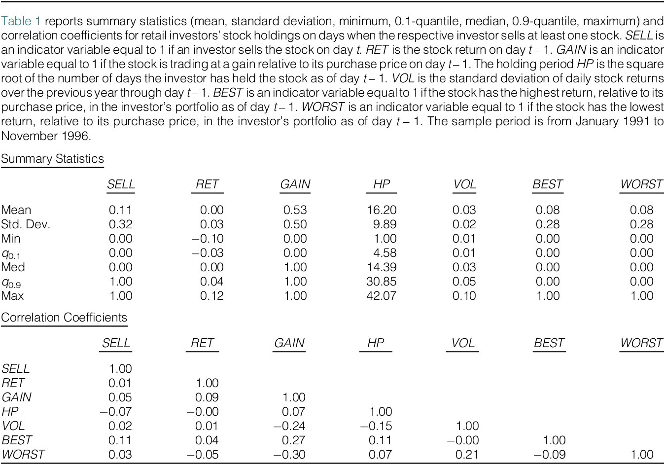
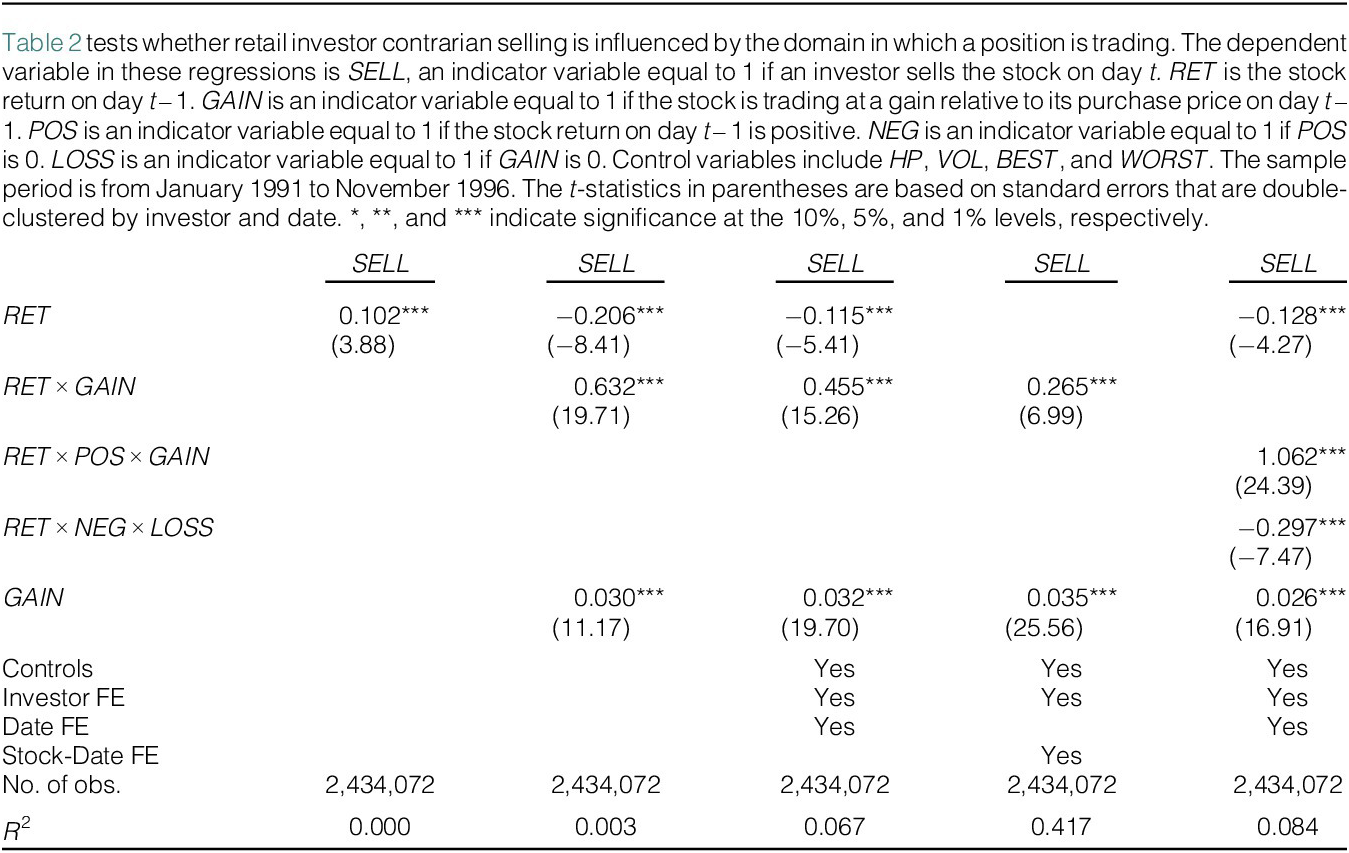


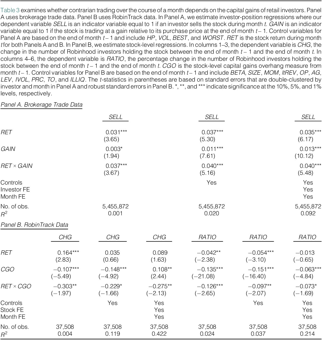
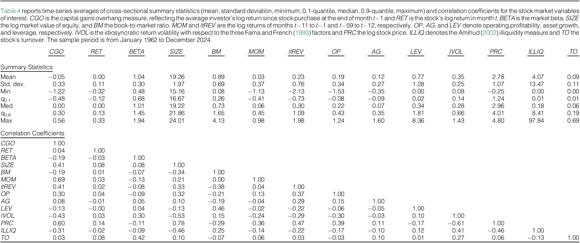
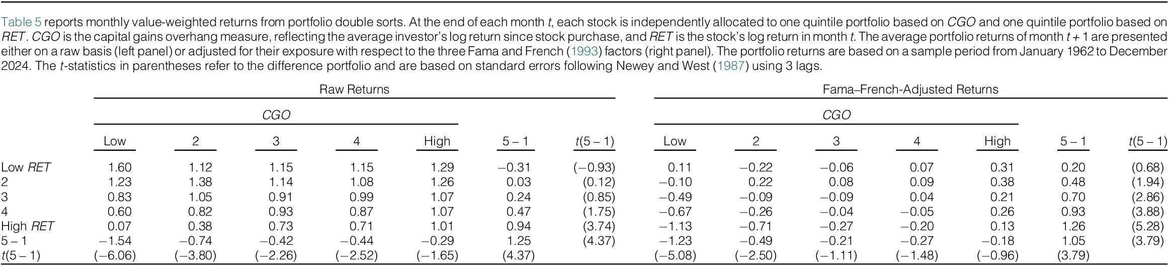
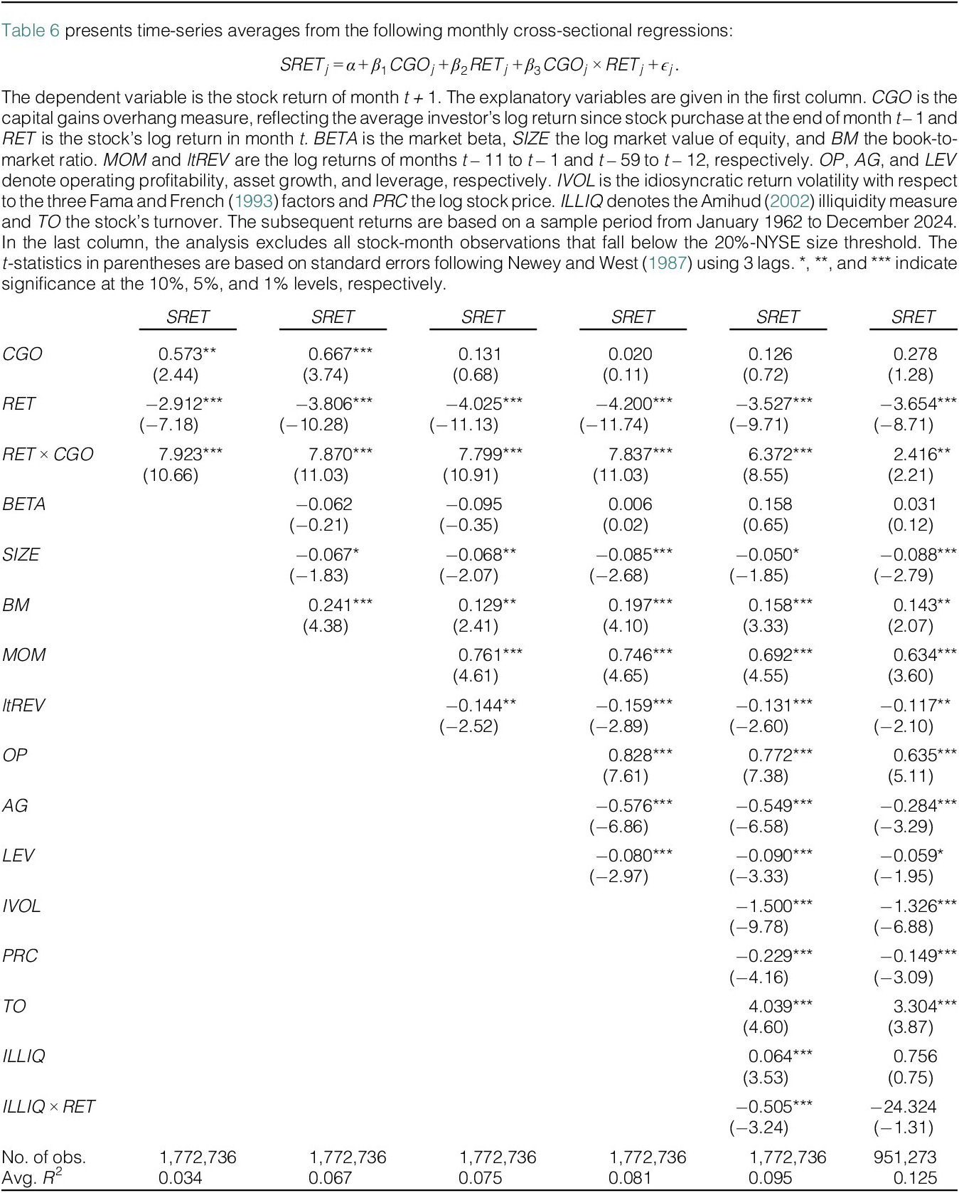
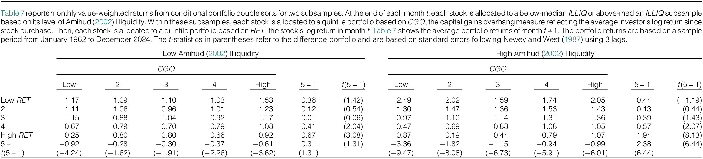
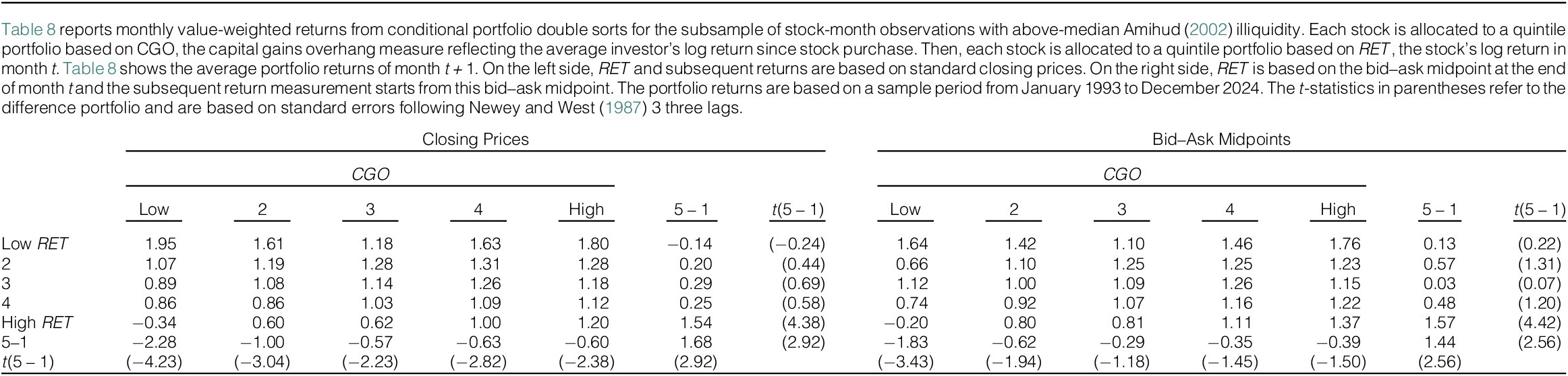
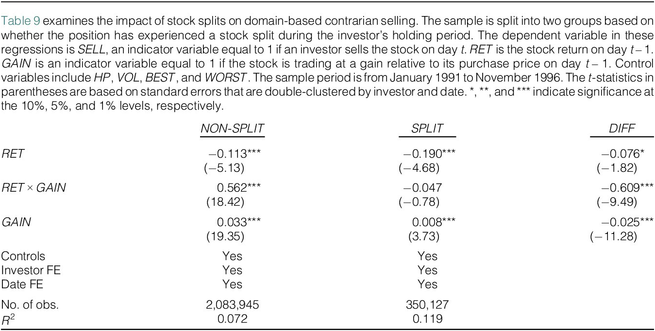
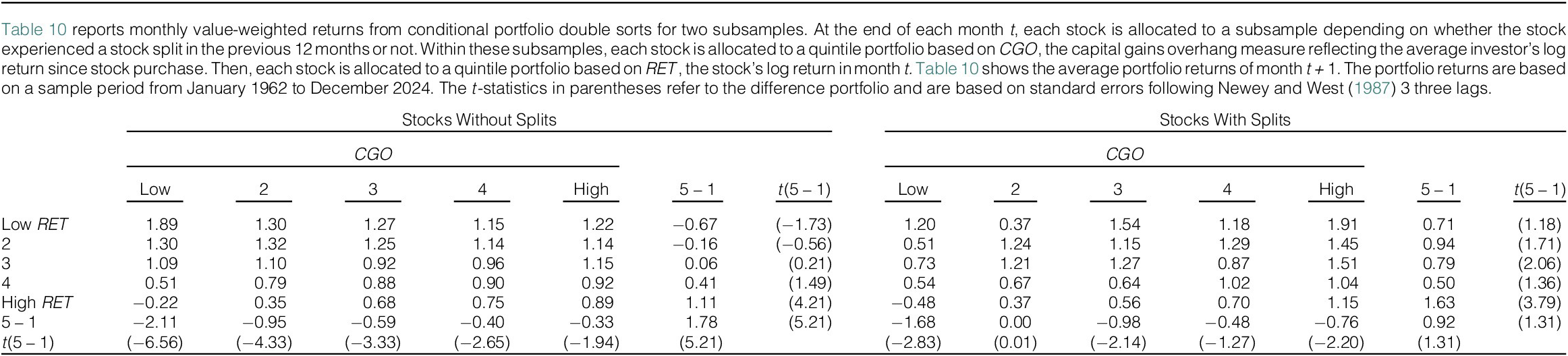


 Open access