


There may, indeed, be other applications of the system than its use as a logic.
——————————————————
A. Church, Postulates for the foundation of logic
1. Introduction
The sequent calculus and the lambda calculus were both invented in the context of logical investigations, the former by Gentzen as a language of proofs (Gentzen, Reference Gentzen1935) and the latter by Church as a language of functions (Church, Reference Church1932). The computational content of these calculi emerged at different times, with the relevance of
 $\beta$
-reduction of lambda terms to the emerging theory of computation being more quickly realised than the relevance of cut-elimination. By now, it is clear that both calculi have logical and computational aspects and that the two calculi are deeply related to one another. In this paper, we revisit this relationship in the form of an isomorphism of categories (Theorem 4.15)
$\beta$
-reduction of lambda terms to the emerging theory of computation being more quickly realised than the relevance of cut-elimination. By now, it is clear that both calculi have logical and computational aspects and that the two calculi are deeply related to one another. In this paper, we revisit this relationship in the form of an isomorphism of categories (Theorem 4.15)

for each sequence
 $\Gamma$
of formulas (née types) where
$\Gamma$
of formulas (née types) where
 $\mathcal{S}_\Gamma$
is a category of proofs in intuitionistic sequent calculus (defined in Section 2) and
$\mathcal{S}_\Gamma$
is a category of proofs in intuitionistic sequent calculus (defined in Section 2) and
 $\mathcal{L}_\Gamma$
is a category of simply-typed lambda terms (defined in Section 3). Both categories have the same set of objects, viewed either as the formulas of intuitionistic propositional logic or simple types. The set of morphisms
$\mathcal{L}_\Gamma$
is a category of simply-typed lambda terms (defined in Section 3). Both categories have the same set of objects, viewed either as the formulas of intuitionistic propositional logic or simple types. The set of morphisms
 $\mathcal{S}_\Gamma (p,q)$
is the set of proofs of
$\mathcal{S}_\Gamma (p,q)$
is the set of proofs of
 $\Gamma \vdash p \supset q$
up to an equivalence relation
$\Gamma \vdash p \supset q$
up to an equivalence relation
 $\sim _p$
generated by cut-elimination transformations and commuting conversions together with a small number of additional natural relations, while
$\sim _p$
generated by cut-elimination transformations and commuting conversions together with a small number of additional natural relations, while
 $\mathcal{L}_\Gamma (p,q)$
is the set of simply-typed lambda terms of type
$\mathcal{L}_\Gamma (p,q)$
is the set of simply-typed lambda terms of type
 $p \rightarrow q$
whose free variables have types taken from
$p \rightarrow q$
whose free variables have types taken from
 $\Gamma$
, taken up to
$\Gamma$
, taken up to
 $\beta \eta$
-equivalence. We refer to this isomorphism of categories and the normal form theorem which refines it (Theorem 4.49) as the Gentzen–Mints–Zucker duality between sequent calculus and lambda calculus. The name reflects work by Zucker (Reference Zucker1974) and Mints (Reference Mints and Odifreddi1996), elaborated below.
$\beta \eta$
-equivalence. We refer to this isomorphism of categories and the normal form theorem which refines it (Theorem 4.49) as the Gentzen–Mints–Zucker duality between sequent calculus and lambda calculus. The name reflects work by Zucker (Reference Zucker1974) and Mints (Reference Mints and Odifreddi1996), elaborated below.
A duality consists of two different points of view on the same object (Atiyah, Reference Atiyah2007). The greater the difference between the two points of view, the more informative is the duality which relates them. Such correspondences are important because two independent discoveries of the same structure are strong evidence that the structure is natural. The above duality is interesting precisely because sequent calculus proofs and lambda terms are not tautologically the same thing: for example, the cut-elimination relations are fundamentally local while the
 $\beta$
-equivalence relation is global (see Section 4.3). In this sense, sequent calculus and lambda calculus are, respectively, local and global points of view on a common logico-computational mathematical structure.
$\beta$
-equivalence relation is global (see Section 4.3). In this sense, sequent calculus and lambda calculus are, respectively, local and global points of view on a common logico-computational mathematical structure.
This duality is related to, but distinct from, the Curry–Howard correspondence. The precise relationship is elaborated in Section 1.1 below, but broadly speaking, it is captured by the conceptual diagram of Figure 1. The Curry–Howard correspondence gives a bijection between natural deduction proofs and lambda terms, while Gentzen–Mints–Zucker duality reveals that
 $\beta \eta$
-normal lambda terms are normal forms for sequent calculus proofs modulo an equivalence relation generated by pairs that are well-motivated from the point of view of the Brouwer-Heyting-Kolmogorov interpretation of intuitionistic proof.
$\beta \eta$
-normal lambda terms are normal forms for sequent calculus proofs modulo an equivalence relation generated by pairs that are well-motivated from the point of view of the Brouwer-Heyting-Kolmogorov interpretation of intuitionistic proof.
The relationship between three logico-computational calculi.

1.1 The Curry–Howard correspondence
The relationship between proofs and lambda terms (or “programs”) has become widely known as the Curry–Howard correspondence following Howard’s work (Howard, Reference Howard1980), although an informal understanding of the computational content of intuitionistic proofs has older roots in the Brouwer–Heyting–Kolmogorov interpretation (Troelstra and van Dalen, Reference Troelstra and van Dalen1988). The correspondence has been so influential in logic and computer science that the Curry–Howard correspondence as philosophy now overshadows the Curry–Howard correspondence as a theorem.
As a theorem, the Curry–Howard correspondence is the observation that the formulas of implicational propositional logic are the same as the types of simply-typed lambda calculus, and that there is a surjective map from the set of all proofs of a sequent
 $\Gamma \vdash \alpha$
in “sequent calculus” to the set of all lambda terms of type
$\Gamma \vdash \alpha$
in “sequent calculus” to the set of all lambda terms of type
 $\alpha$
with free variables in
$\alpha$
with free variables in
 $\Gamma$
(due to Howard (Reference Howard1980, Section 3) building on ideas of Curry and Tait). This map is not a bijection, and as such does not represent the best possible statement about the relationship between proofs and lambda terms. The problem is that there are two natural continuations of Howard’s work, depending on how one interprets the somewhat vague notion of proof in Howard (Reference Howard1980, Section 1).
$\Gamma$
(due to Howard (Reference Howard1980, Section 3) building on ideas of Curry and Tait). This map is not a bijection, and as such does not represent the best possible statement about the relationship between proofs and lambda terms. The problem is that there are two natural continuations of Howard’s work, depending on how one interprets the somewhat vague notion of proof in Howard (Reference Howard1980, Section 1).
The vagueness is due to the fact that the system called “sequent calculus” by Howard is actually a hybrid of intuitionistic sequent calculus in the sense of Gentzen’s LJ (there are weakening, exchange and contraction rules in Howard’s system) and natural deduction in the sense of Gentzen (Reference Gentzen1935) and Prawitz (Reference Prawitz1965) (Howard has an elimination rule for implication rather than the left introduction rule of sequent calculus). The use of an elimination rule makes the connection to lambda terms straightforward, and the inclusion of structural rules places the correspondence in its proper context as a relationship between proofs with hypotheses and lambda terms with free variables (Howard, Reference Howard1980, Section 3).
In resolving this ambiguity, subsequent authors writing about the correspondence have almost universally decided that proof means natural deduction proof; see, for example, (Sørensen and Urzyczyn, Reference Sørensen and Urzyczyn2006, Sections 4.8, 7.4, 7.6) and Wadler (Reference Wadler2000). The correspondence may then be interpreted as a bijection between lambda terms and natural deduction proofs (Selinger, Reference Selinger2008, Section 6.5). This bijection represents the natural conclusion of one line of development starting with Howard (Reference Howard1980), and henceforth we refer to this bijection as the Curry–Howard correspondence. Despite its philosophical importance, this correspondence is not mathematically of great interest, because natural deduction and lambda calculus are so similar that the bijection is close to tautological (in the case of closed terms, it is left as an exercise in one standard text (Sørensen and Urzyczyn, Reference Sørensen and Urzyczyn2006, Ex. 4.8)).
In the present work, we investigate the second natural continuation of Howard (Reference Howard1980), which takes the structural rules in Howard’s “sequent calculus” seriously and seeks to give a bijection between sequent calculus proofs and lambda terms. As soon as explicit structural rules are introduced into proofs, however, there will be multiple proofs that map to the same lambda term, and so for there to be a bijection between proofs and lambda terms, proof must mean equivalence class of preproofs modulo some relation. If this relation is simply “maps to the same lambda term,” then what we have constructed is merely a surjective map from proofs to lambda terms, which is hardly more than what is in Howard (Reference Howard1980). Hence, in this second line of thought, the identity of proofs becomes a central concern.
Consequently one of the contributions of this paper is to give explicit generating relations for a relation
 $\sim _p$
on preproofs such that
$\sim _p$
on preproofs such that
 $\pi _1 \sim _p \pi _2$
if and only if
$\pi _1 \sim _p \pi _2$
if and only if
 $F_\Gamma (\pi _1) = F_\Gamma (\pi _2)$
, and to give a logical justification of these relations independent of the translation to lambda terms. This establishes
$F_\Gamma (\pi _1) = F_\Gamma (\pi _2)$
, and to give a logical justification of these relations independent of the translation to lambda terms. This establishes
 $\mathcal{S}_\Gamma$
as a mathematical structure in its own right, so that the comparison to
$\mathcal{S}_\Gamma$
as a mathematical structure in its own right, so that the comparison to
 $\mathcal{L}_\Gamma$
may be meaningfully referred to as a duality.
$\mathcal{L}_\Gamma$
may be meaningfully referred to as a duality.
Given the Curry–Howard correspondence, the identity of proofs is closely related to the old problem of when two sequent calculus proofs map to the same natural deduction under the translation defined by Gentzen (Reference Gentzen1935) (see Remark 4.5). This has been studied by various authors, most notably (Zucker, Reference Zucker1974; Pottinger, Reference Pottinger1977; Dyckhoff and Pinto, Reference Dyckhoff and Pinto1999; Mints, Reference Mints and Odifreddi1996; Kleene, Reference Kleene1952). The most important results are those obtained by Zucker and Mints, and we restrict ourselves here to comments on their work; see also Section 4.4.
There is substantial overlap between our main results and those of Zucker and Mints, which we became aware of after this paper had been completed. In Zucker (Reference Zucker1974), Zucker gives a set of generating relations characterising when two sequent calculus proofs map to the same natural deduction, for a calculus that does not contain weakening and exchange. The main content of Theorem 4.15 also lies in identifying an explicit set of generating relations on preproofs, for the map from sequent calculus proofs to lambda terms in a system of sequent calculus that is (as far as is possible for a system that must be translated unambiguously to lambda terms) as close as possible to Gentzen’s LJ. As far as we know, this paper is the first place where the generating relations have been established for Gentzen’s LJ with all structural rules.
Mints, using ideas of Kleene (Reference Kleene1952), identifies a set of normal forms of sequent calculus proofs and studies them using the map from proofs to lambda terms. Our proof of the main theorem (Theorem 4.15) relies on the identification of normal forms, which differ slightly from those of Mints (see also Theorem 4.49). Again, we treat a standard form of LJ, whereas Mints (Reference Mints and Odifreddi1996) follows Kleene’s system G (Kleene, Reference Kleene1952) in the form of its
 $(L \supset\!)$
rule.
$(L \supset\!)$
rule.
Finally, since we must argue that
 $\mathcal{S}_\Gamma$
has an independent existence in order for the duality to be a relationship between equals, we are committed to mounting a purely logical defence of all the generating relations of
$\mathcal{S}_\Gamma$
has an independent existence in order for the duality to be a relationship between equals, we are committed to mounting a purely logical defence of all the generating relations of
 $\sim _p$
. This is not a concern shared by Zucker, Mints or Kleene. The most interesting generating relations are those that we call
$\sim _p$
. This is not a concern shared by Zucker, Mints or Kleene. The most interesting generating relations are those that we call
 $\lambda$
-equivalences (Definition 2.21) which, are justified on the grounds that they represent an internal Brouwer-Heyting-Kolmogorov interpretation, see the discussion preceding Definition 2.21 and Section 4.2.
$\lambda$
-equivalences (Definition 2.21) which, are justified on the grounds that they represent an internal Brouwer-Heyting-Kolmogorov interpretation, see the discussion preceding Definition 2.21 and Section 4.2.
The connection between syntactic presentations of proofs and their categorical semantics, as developed in foundational work by Lambek (Reference Lambek1958, 1969), Scott (Reference Scott1976), Scott et al. (1980), Seely (Reference Seely1984, Reference Seely1989), and others, is indeed central to our perspective. In particular, the categories
 $\mathcal{L}_\Gamma$
and
$\mathcal{L}_\Gamma$
and
 $\mathcal{S}_\Gamma$
can be understood as presentations of the free cartesian closed category generated by
$\mathcal{S}_\Gamma$
can be understood as presentations of the free cartesian closed category generated by
 $\Gamma$
, and our main equivalence theorem reflects the fact that the simply-typed lambda calculus and the intuitionistic sequent calculus provide distinct but equivalent syntactic lenses on the same semantic object. While we focus on a syntactic account of proof equivalence, the internal BHK semantics developed in Section 4.2 is closely aligned with categorical models of proofs: for instance, our treatment echoes the coherence conditions familiar from cartesian closed categories. We believe these connections offer promising directions for future work, particularly in relating our equivalence results to existing coherence theorems in categorical proof theory.
$\Gamma$
, and our main equivalence theorem reflects the fact that the simply-typed lambda calculus and the intuitionistic sequent calculus provide distinct but equivalent syntactic lenses on the same semantic object. While we focus on a syntactic account of proof equivalence, the internal BHK semantics developed in Section 4.2 is closely aligned with categorical models of proofs: for instance, our treatment echoes the coherence conditions familiar from cartesian closed categories. We believe these connections offer promising directions for future work, particularly in relating our equivalence results to existing coherence theorems in categorical proof theory.
2. Sequent Calculus
We introduce the Sequent Calculus system (Gentzen’s LJ) and define a family of equivalence relations on proofs within this system. These equivalence relations are summarised in Table 1.
Summary of equivalence relations and their justifications

In this paper, we restrict our attention to the intuitionistic sequent calculus with implication, for simplicity. The inclusion of additional connectives, such as conjunctions and disjunctions, is left for future work.
There is an infinite set of atomic formulas, and if
 $p$
and
$p$
and
 $q$
are formulas, then so is
$q$
are formulas, then so is
 $p \supset q$
. Let
$p \supset q$
. Let
 $\Psi _\supset$
denote the set of all formulas. For each formula
$\Psi _\supset$
denote the set of all formulas. For each formula
 $p$
, let
$p$
, let
 $Y_p$
be an infinite set of variables associated with
$Y_p$
be an infinite set of variables associated with
 $p$
. For distinct formulas
$p$
. For distinct formulas
 $p,q$
, the sets
$p,q$
, the sets
 $Y_p, Y_q$
are disjoint. We write
$Y_p, Y_q$
are disjoint. We write
 $x : p$
for
$x : p$
for
 $x \in Y_p$
and say
$x \in Y_p$
and say
 $x$
has type
$x$
has type
 $p$
. Let
$p$
. Let
 $\mathcal{P}^n$
be the set of all length
$\mathcal{P}^n$
be the set of all length
 $n$
sequences of variables with
$n$
sequences of variables with
 $\mathcal{P}^0 := \lbrace \varnothing \rbrace$
, and
$\mathcal{P}^0 := \lbrace \varnothing \rbrace$
, and
 $\mathcal{P} := \cup _{n = 0}^\infty \mathcal{P}^n$
. A sequent is a pair
$\mathcal{P} := \cup _{n = 0}^\infty \mathcal{P}^n$
. A sequent is a pair
 $(\Gamma ,p)$
where
$(\Gamma ,p)$
where
 $\Gamma \in \mathcal{P}$
and
$\Gamma \in \mathcal{P}$
and
 $p \in \Psi _\supset$
, written
$p \in \Psi _\supset$
, written
 $\Gamma \vdash p$
. We call
$\Gamma \vdash p$
. We call
 $\Gamma$
the antecedent and
$\Gamma$
the antecedent and
 $p$
the succedent of the sequent. Given
$p$
the succedent of the sequent. Given
 $\Gamma$
and a variable
$\Gamma$
and a variable
 $x:p$
, we write
$x:p$
, we write
 $\Gamma , x:p$
for the element of
$\Gamma , x:p$
for the element of
 $\mathcal{P}$
given by appending
$\mathcal{P}$
given by appending
 $x:p$
to the end of
$x:p$
to the end of
 $\Gamma$
. A variable
$\Gamma$
. A variable
 $x:p$
may occur more than once in a sequent.
$x:p$
may occur more than once in a sequent.
Our intuitionistic sequent calculus is the system LJ of Gentzen (Reference Gentzen1935, Section III) restricted to implication, with formulas in the antecedent tagged with variables. We follow the convention of Girard et al. (Reference Girard, Lafont and Taylor1989, Section 5.1) in grouping
 $(\!\operatorname {ax}\!)$
and
$(\!\operatorname {ax}\!)$
and
 $(\!\operatorname {cut}\!)$
together rather than including the latter in the structural rules.
$(\!\operatorname {cut}\!)$
together rather than including the latter in the structural rules.
Definition 2.1.
A deduction rule results from one of the schemata below by a substitution of the following kind: replace
 $p,q,r$
by arbitrary formulas,
$p,q,r$
by arbitrary formulas,
 $x,y$
by arbitrary variables, and
$x,y$
by arbitrary variables, and
 $\Gamma , \Delta , \Theta$
by arbitrary (possibly empty) sequences of formulas separated by commas:
$\Gamma , \Delta , \Theta$
by arbitrary (possibly empty) sequences of formulas separated by commas:
-
• the identity group :
-
– Axiom :

-
– Cut :
-
-
• the structural rules :
-
– Contraction :
-
– Weakening :
-
– Exchange :
-
-
• the logical rules :
-
– Right introduction :
-
– Left introduction :
-


Definition 2.2.
A preproof is a finite rooted planar tree where each edge is labelled by a sequent and each node except for the root is labelled by a valid deduction rule. If the edge connected to the root is labelled by the sequent
 $\Gamma \vdash p$
then we call the preproof a preproof of
$\Gamma \vdash p$
then we call the preproof a preproof of
 $\Gamma \vdash p$
.
$\Gamma \vdash p$
.
Observe that the only valid label for a leaf node is an axiom rule, so a preproof reads from the leaves to the root as a deduction of
 $\Gamma \vdash p$
from axiom rules.
$\Gamma \vdash p$
from axiom rules.
Example 2.3.
Here is the Church numeral
 $\underline {2}$
in our sequent calculus
$\underline {2}$
in our sequent calculus

Remark 2.4. Multiple occurrences of a deduction rule are represented using doubled horizontal lines. For example if
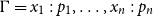 $\Gamma = x_1: p_1, \ldots , x_n: p_n$
then the preproof
$\Gamma = x_1: p_1, \ldots , x_n: p_n$
then the preproof

weakens in every formula in the sequence. The doubled horizontal line therefore stands for
 $n$
occurrences of the rule
$n$
occurrences of the rule
 $(\!\operatorname {weak}\!)$
. The preproofs which perform these weakenings in a different order are, of course, not equal as preproofs, so the notation is an abuse. We will only use it below in the context of defining generating pairs of equivalence relations in cases where any reading of this notation leads to the same equivalence relation.
$(\!\operatorname {weak}\!)$
. The preproofs which perform these weakenings in a different order are, of course, not equal as preproofs, so the notation is an abuse. We will only use it below in the context of defining generating pairs of equivalence relations in cases where any reading of this notation leads to the same equivalence relation.
Remark 2.5. We follow Gentzen (Reference Gentzen1935, Section III) in putting the variable introduced by a
 $(L \supset\!)$
rule at the first position in the antecedent. This choice is correct from the point of view of the relationship between sequent calculus proofs and lambda terms, as may be seen in Lemma 4.29 and Section 4.1.
$(L \supset\!)$
rule at the first position in the antecedent. This choice is correct from the point of view of the relationship between sequent calculus proofs and lambda terms, as may be seen in Lemma 4.29 and Section 4.1.
When should two preproofs be considered to be the same proof? Clearly some of the structure of a preproof is logically insignificant, but it is by no means trivial to identify a precise notion of proof as separate from preproof. Historically, logic has concerned itself primarily with the provability of sequents
 $\Gamma \vdash p$
rather than the structure of the set of all preproofs, but as proof theory has developed the question of the identity of proofs has acquired increasing importance; see Ungar (1992) and Prawitz (Reference Prawitz1981, Section 4.3). We also note the foundational contributions of G. Kreisel, who in his influential works Kreisel (Reference Kreisel1962, Reference Kreisel and Saaty1965) suggested to distinguish the “Theory of Proofs” (that studies the proofs as individual entities, close to the approach of this paper) and “Proof Theory”.
$\Gamma \vdash p$
rather than the structure of the set of all preproofs, but as proof theory has developed the question of the identity of proofs has acquired increasing importance; see Ungar (1992) and Prawitz (Reference Prawitz1981, Section 4.3). We also note the foundational contributions of G. Kreisel, who in his influential works Kreisel (Reference Kreisel1962, Reference Kreisel and Saaty1965) suggested to distinguish the “Theory of Proofs” (that studies the proofs as individual entities, close to the approach of this paper) and “Proof Theory”.
We say that a relation
 $\sim$
on the set of preproofs satisfies condition (C0) if
$\sim$
on the set of preproofs satisfies condition (C0) if
 $\pi _1 \sim \pi _2$
implies
$\pi _1 \sim \pi _2$
implies
 $\pi _1, \pi _2$
are preproofs of the same sequent. The relation satisfies condition (C1) if it satisfies (C0) and
$\pi _1, \pi _2$
are preproofs of the same sequent. The relation satisfies condition (C1) if it satisfies (C0) and
 $\pi _1 \sim \pi _2$
implies
$\pi _1 \sim \pi _2$
implies
 $\pi _1' \sim \pi _2'$
where
$\pi _1' \sim \pi _2'$
where
 $\pi _1', \pi _2'$
are the result of applying the same deduction rule to
$\pi _1', \pi _2'$
are the result of applying the same deduction rule to
 $\pi _1, \pi _2$
, respectively. For example, if
$\pi _1, \pi _2$
, respectively. For example, if
 $\sim$
satisfies (C1) and
$\sim$
satisfies (C1) and
 $\pi _1 \sim \pi _2$
then
$\pi _1 \sim \pi _2$
then

Condition (C2) is defined using the following schematics:

We say that a relation
 $\sim$
on the set of preproofs satisfies condition (C2) if it satisfies (C0) and whenever
$\sim$
on the set of preproofs satisfies condition (C2) if it satisfies (C0) and whenever
 $\pi _1 \sim \pi _2$
and
$\pi _1 \sim \pi _2$
and
 $\rho _1 \sim \rho _2$
then also
$\rho _1 \sim \rho _2$
then also
 $\kappa _1 \sim \kappa _2$
where
$\kappa _1 \sim \kappa _2$
where
 $\kappa _i$
for
$\kappa _i$
for
 $i \in \{1,2\}$
is obtained from the pair
$i \in \{1,2\}$
is obtained from the pair
 $(\pi _i, \rho _i)$
by application of one of the deduction rules in (2.1).
$(\pi _i, \rho _i)$
by application of one of the deduction rules in (2.1).
Definition 2.6.
A relation
 $\sim$
on preproofs is compatible if it satisfies (C0),(C1),(C2).
$\sim$
on preproofs is compatible if it satisfies (C0),(C1),(C2).
An occurrence of
 $x:p$
in a preproof
$x:p$
in a preproof
 $\pi$
is an occurrence in the antecedent
$\pi$
is an occurrence in the antecedent
 $\Gamma$
of a sequent labelling some edge of
$\Gamma$
of a sequent labelling some edge of
 $\pi$
. Some occurrences are related by the flow of information in the preproof, and some are not. More precisely:
$\pi$
. Some occurrences are related by the flow of information in the preproof, and some are not. More precisely:
Definition 2.7 (Ancestors). An occurrence of
 $z_1:s$
in a preproof
$z_1:s$
in a preproof
 $\pi$
is an immediate strong ancestor (resp. immediate weak ancestor) of an occurrence
$\pi$
is an immediate strong ancestor (resp. immediate weak ancestor) of an occurrence
 $z_2:s$
if there is a deduction rule in
$z_2:s$
if there is a deduction rule in
 $\pi$
where
$\pi$
where
 $z_1:s$
is in the numerator and
$z_1:s$
is in the numerator and
 $z_2:s$
is in the denominator, and one of the following holds (referring to the schemata in Definition 2.1):
$z_2:s$
is in the denominator, and one of the following holds (referring to the schemata in Definition 2.1):
-
(i)
$z_1:s, z_2:s$
are in the same position of
$\Gamma , \Delta , \Theta$
in the numerator and denominator.
-
(ii) the rule is
$(\!\operatorname {ctr}\!)$
,
$z_1:s$
is the first of the two variables being contracted (resp.
$z_1:s$
is either of the variables being contracted) and
$z_2:s$
is the result of that contraction.
-
(iii) the rule is
$(\!\operatorname {ex}\!)$
and either
$z_1:s = x:p, z_2:s = x:p$
or
$z_1:s = y:p, z_2:s = y:p$
.


One occurrence
 $z:s$
is a strong ancestor (resp. weak ancestor) of another
$z:s$
is a strong ancestor (resp. weak ancestor) of another
 $z':s$
if there is a sequence
$z':s$
if there is a sequence
 $z:s = z_1:s, \ldots , z_n:s = z':s$
of occurrences in
$z:s = z_1:s, \ldots , z_n:s = z':s$
of occurrences in
 $\pi$
with
$\pi$
with
 $z_i:s$
an immediate strong (resp. weak) ancestor of
$z_i:s$
an immediate strong (resp. weak) ancestor of
 $z_{i+1}:s$
for
$z_{i+1}:s$
for
 $1 \le i \lt n$
.
$1 \le i \lt n$
.
Note that if
 $z_1:s$
is a strong ancestor of
$z_1:s$
is a strong ancestor of
 $z_2:s$
then
$z_2:s$
then
 $z_1 = z_2$
but this is not necessarily true for weak ancestors.
$z_1 = z_2$
but this is not necessarily true for weak ancestors.
Definition 2.8.
Let
 $\approx _{str}$
(resp.
$\approx _{str}$
(resp.
 $\approx _{wk}$
) denote the equivalence relation on the set of variable occurrences generated by the strong (resp. weak) ancestor relation.
$\approx _{wk}$
) denote the equivalence relation on the set of variable occurrences generated by the strong (resp. weak) ancestor relation.
Definition 2.9 (Ancestor substitution). Let
 $x:p$
be an occurrence of a variable in a preproof
$x:p$
be an occurrence of a variable in a preproof
 $\pi$
and
$\pi$
and
 $y:p$
another variable. We denote by
$y:p$
another variable. We denote by
 $\operatorname {subst}^{str}(\pi , x, y)$
the preproof obtained from
$\operatorname {subst}^{str}(\pi , x, y)$
the preproof obtained from
 $\pi$
by replacing the occurrence
$\pi$
by replacing the occurrence
 $x:p$
and all its strong ancestors by
$x:p$
and all its strong ancestors by
 $y$
.
$y$
.
Example 2.10.
In the preproof
 $\underline {2}$
of Example 2.3 the partition of variable occurrences according to the equivalence relation
$\underline {2}$
of Example 2.3 the partition of variable occurrences according to the equivalence relation
 $\approx _{str}$
is shown by colours in
$\approx _{str}$
is shown by colours in

and the partition according to
 $\approx _{wk}$
in
$\approx _{wk}$
in

In our preproofs, we have tags, in the form of variables, for hypotheses. Since the precise nature of these tags is immaterial, if the variable is eliminated in a
 $(R \supset\!)$
,
$(R \supset\!)$
,
 $(L \supset\!)$
,
$(L \supset\!)$
,
 $(\!\operatorname {ctr}\!)$
or
$(\!\operatorname {ctr}\!)$
or
 $(\!\operatorname {cut}\!)$
rule the identity of the proof should be independent of the tag. Thus we define
$(\!\operatorname {cut}\!)$
rule the identity of the proof should be independent of the tag. Thus we define
 $\alpha$
-equivalence to formalise this. See Definition A.1.
$\alpha$
-equivalence to formalise this. See Definition A.1.
Remark 2.11. The generating relation (A.4) of Definiton A.1 is to be read as a pair of preproofs
 $(\psi ,\psi ') \in \; \sim _\alpha$
where both preproofs have final sequent
$(\psi ,\psi ') \in \; \sim _\alpha$
where both preproofs have final sequent
 $z: p \supset q, \Gamma , \Delta , \Theta \vdash r$
and the branch ending in
$z: p \supset q, \Gamma , \Delta , \Theta \vdash r$
and the branch ending in
 $\Gamma \vdash p$
is any preproof (but it is the same preproof in both
$\Gamma \vdash p$
is any preproof (but it is the same preproof in both
 $\psi$
and
$\psi$
and
 $\psi '$
). To avoid clutter, we will not label branches, here or elsewhere, if it is clear how to match up the branches in the two preproofs involved in the relation.
$\psi '$
). To avoid clutter, we will not label branches, here or elsewhere, if it is clear how to match up the branches in the two preproofs involved in the relation.
Multiple distinct sequences of applications of
 $(\!\operatorname {ex}\!)$
rules can yield the same permutation of formulas within a hypothesis. We establish an equivalence relation to identify these.
$(\!\operatorname {ex}\!)$
rules can yield the same permutation of formulas within a hypothesis. We establish an equivalence relation to identify these.
Definition 2.12 (
 $\operatorname {ex}$
-Equivalence). We define
$\operatorname {ex}$
-Equivalence). We define
 $\sim _{(\!\operatorname {ex}\!)}$
to be the smallest compatible equivalence relation on preproofs satisfying the following (recall our conventions with double horizontal lines of Remark 2.4)
$\sim _{(\!\operatorname {ex}\!)}$
to be the smallest compatible equivalence relation on preproofs satisfying the following (recall our conventions with double horizontal lines of Remark 2.4)

where
 $\tau$
is a permutation and
$\tau$
is a permutation and
 $\sigma _1, \ldots , \sigma _r$
and
$\sigma _1, \ldots , \sigma _r$
and
 $\rho _1,\ldots ,\rho _s$
are sequences of transpositions of consecutive positions (one or both lists may be empty) with the property that
$\rho _1,\ldots ,\rho _s$
are sequences of transpositions of consecutive positions (one or both lists may be empty) with the property that
 $\sigma _1 \cdots \sigma _r = \tau = \rho _1 \cdots \rho _s$
in the permutation group. The two preproofs in (
2.2
) are, respectively, the sequences of exchanges corresponding to the
$\sigma _1 \cdots \sigma _r = \tau = \rho _1 \cdots \rho _s$
in the permutation group. The two preproofs in (
2.2
) are, respectively, the sequences of exchanges corresponding to the
 $\sigma _i$
and
$\sigma _i$
and
 $\rho _j$
.
$\rho _j$
.
In this paper, we present many conversion rules relating preproofs which only differ by logically insignificant rearrangements of deduction rules. The system we have adopted holds a strict set of rules which only allow
 $(\!\operatorname {cut}\!), (\!\operatorname {ctr}\!), (\!\operatorname {weak}\!), (L\supset\!), (L\supset\!)$
rules where the relevant formula is on the far left of the sequent. Upholding this for the remainder of the paper will make the logical content of the conversion rules less transparent than if we work with a more liberal system involving derived rules. Thus, we introduce the following.
$(\!\operatorname {cut}\!), (\!\operatorname {ctr}\!), (\!\operatorname {weak}\!), (L\supset\!), (L\supset\!)$
rules where the relevant formula is on the far left of the sequent. Upholding this for the remainder of the paper will make the logical content of the conversion rules less transparent than if we work with a more liberal system involving derived rules. Thus, we introduce the following.
Definition 2.13. The following derived rules are the extended deduction rules, where by a slight abuse of notation, we give the same names as the strict counterparts given in Definition 2.1 :
-
• the identity group :
-
– Cut :
-
-
• the structural rules :
-
– Contraction :
-
– Weakening :
-
-
• the logical rules :
-
– Right introduction :
-
– Left introduction :
-


Example 2.14. As an example of how these derived rules are derived, consider the Contraction rule, which stands for the following deduction:

Notice that any two such preproof fragments are equivalent under
 $(\!\operatorname {ex}\!)$
-equivalence (Definition 2.12).
$(\!\operatorname {ex}\!)$
-equivalence (Definition 2.12).
We will work with these derived rules for the remainder of this paper. More precisely, we replace the deduction rules of Definition 2.1 with the same name as those of Definition 2.13 with those of Definition 2.13. This is a more liberal system than the strict version of Gentzen’s LJ, but the payoff is that the local nature of sequent calculus is made significantly more transparent, which is a perspective we wish to emphasise. We include the following equivalences which allow the purist to relate our more liberal system to the more strict one, see Lemma 2.17.
The price for our more liberal deduction rules is the inclusion of
 $\tau$
-equivalences below, which express that two instances of the same deduction rule, operating in different places, are essentially the same.
$\tau$
-equivalences below, which express that two instances of the same deduction rule, operating in different places, are essentially the same.
Definition 2.15 (
 $\tau$
-Equivalence). We define
$\tau$
-Equivalence). We define
 $\sim _{\tau }$
to be the smallest compatible equivalence relation on preproofs satisfying
$\sim _{\tau }$
to be the smallest compatible equivalence relation on preproofs satisfying


Definition 2.16.
A deduction rule is strict if it is an arbitrary
 $(\!\operatorname {ax}\!)$
or
$(\!\operatorname {ax}\!)$
or
 $(\!\operatorname {ex}\!)$
rule, or it is one of the other rules and the occurrence of
$(\!\operatorname {ex}\!)$
rule, or it is one of the other rules and the occurrence of
 $x:p$
in the rule is leftmost in the antecedent. A strict preproof is a preproof in which every deduction rule is strict.
$x:p$
in the rule is leftmost in the antecedent. A strict preproof is a preproof in which every deduction rule is strict.
Lemma 2.17.
Every preproof is equivalent under
 $\sim _\tau$
to a strict preproof.
$\sim _\tau$
to a strict preproof.
We have a strong intuition about the structure of logical arguments which leads to the expectation that the antecedent of a sequent is an extended “space” disjoint subsets of which may be the locus of independent operations. This independence is formalised by commuting conversions, which identify preproofs that differ only by “insignificant” rearranging of deduction rules. These are given in full in Definition A.2.
Should the order of two variables
 $x:p,y:p$
that are contracted be logically significant? We are prevented from identifying contraction on
$x:p,y:p$
that are contracted be logically significant? We are prevented from identifying contraction on
 $x:p,y:p$
with contraction on
$x:p,y:p$
with contraction on
 $y:p,x:p$
because the former leaves
$y:p,x:p$
because the former leaves
 $x:p$
and the latter
$x:p$
and the latter
 $y:p$
, but a sufficient cocommutativity principle is expressed by (2.9). Similarly (2.8) expresses that contraction is coassociative. The rule (2.10) is counitality, which says that we attach no logical meaning to contraction with a variable which has been weakened in. These principles assert that contraction is coalgebraic, a point of view further ramified in linear logic.
$y:p$
, but a sufficient cocommutativity principle is expressed by (2.9). Similarly (2.8) expresses that contraction is coassociative. The rule (2.10) is counitality, which says that we attach no logical meaning to contraction with a variable which has been weakened in. These principles assert that contraction is coalgebraic, a point of view further ramified in linear logic.
Definition 2.18 (
 $co$
-Equivalence). We define
$co$
-Equivalence). We define
 $\sim _{co}$
to be the smallest compatible equivalence relation on preproofs satisfying
$\sim _{co}$
to be the smallest compatible equivalence relation on preproofs satisfying


Remark 2.19. The relation (2.8) appears as the contraction conversion (Zucker, Reference Zucker1974, Section 3.1.2 (b)(i)) of Zucker. The sequent calculus of Zucker (Reference Zucker1974) does not contain explicit weakening or exchange so the relations there do not include (2.9) or (2.10). This omission obscures the coalgebraic structure, which we believe to be an important logical principle.

Principles (2.11) and (2.12) below are of profound importance, as they are the internal manifestation in our system of the Brouwer-Heyting-Kolmogorov interpretation of proofs in intuitionistic logic (Troelstra and van Dalen, Reference Troelstra and van Dalen1988). Under that interpretation, a proof of a hypothesis
 $y: p \supset q$
reads as a transformation of proofs of
$y: p \supset q$
reads as a transformation of proofs of
 $p$
to proofs of
$p$
to proofs of
 $q$
. Rule (2.11) expresses that if the output proof of
$q$
. Rule (2.11) expresses that if the output proof of
 $q$
is to be used multiple times the transformation must be employed once for each copy. Rule (2.12) expresses that if the output is not needed, neither is the transformation nor any of its inputs. Note that these principles mirror (2.19) and (2.20) and therefore in some sense realise
$q$
is to be used multiple times the transformation must be employed once for each copy. Rule (2.12) expresses that if the output is not needed, neither is the transformation nor any of its inputs. Note that these principles mirror (2.19) and (2.20) and therefore in some sense realise
 $(L \supset\!)$
as an internalised cut. We develop this point of view more systematically in Section 4.2.
$(L \supset\!)$
as an internalised cut. We develop this point of view more systematically in Section 4.2.
Definition 2.21 (
 $\lambda$
-equivalence). We define
$\lambda$
-equivalence). We define
 $\sim _{\lambda }$
to be the smallest compatible equivalence relation on preproofs satisfying
$\sim _{\lambda }$
to be the smallest compatible equivalence relation on preproofs satisfying


Remark 2.22. The relation (2.11) appears as contraction conversion (Zucker, Reference Zucker1974, Section 3.1.2 (b)(iii)) of Zucker. The sequent calculus of Zucker (Reference Zucker1974) does not contain explicit weakening so the relations there do not include (2.12). The relation (2.11) is also implicit in Kleene (Reference Kleene1952, Lemma 12) and Mints (Reference Mints and Odifreddi1996, Lemma 2) and (2.12) is implicit in Kleene (Reference Kleene1952, Lemma 4) and Mints (Reference Mints and Odifreddi1996, Lemma 1).
Let us consider the assertion that
 $(\!\operatorname {ax}\!)$
, which, in our system, is available for any formula
$(\!\operatorname {ax}\!)$
, which, in our system, is available for any formula
 $p$
, should be restricted to atomic formulas. Let
$p$
, should be restricted to atomic formulas. Let
 $\Sigma ^\Gamma _q$
denote the set of preproofs of
$\Sigma ^\Gamma _q$
denote the set of preproofs of
 $\Gamma \vdash q$
under our system and
$\Gamma \vdash q$
under our system and
 $\Pi ^\Gamma _q$
the set of preproofs under this system with a restricted axiom rule. Clearly
$\Pi ^\Gamma _q$
the set of preproofs under this system with a restricted axiom rule. Clearly
 $\Pi ^\Gamma _q \subseteq \Sigma ^\Gamma _q$
and if
$\Pi ^\Gamma _q \subseteq \Sigma ^\Gamma _q$
and if
 $\Sigma ^\Gamma _q$
is nonempty then so is
$\Sigma ^\Gamma _q$
is nonempty then so is
 $\Pi ^\Gamma _q$
. Since the restriction on the axiom rule does not affect provability, we are free to adopt it, either directly by changing the deduction rules, or indirectly by keeping the deduction rules as given but adopting an equivalence relation on preproofs which effectively makes the axiom rule on compound formulas a derived rule:
$\Pi ^\Gamma _q$
. Since the restriction on the axiom rule does not affect provability, we are free to adopt it, either directly by changing the deduction rules, or indirectly by keeping the deduction rules as given but adopting an equivalence relation on preproofs which effectively makes the axiom rule on compound formulas a derived rule:
Definition 2.23 (
 $\eta$
-Equivalence). We define
$\eta$
-Equivalence). We define
 $\sim _\eta$
to be the smallest compatible equivalence relation on preproofs such that for arbitrary formulas
$\sim _\eta$
to be the smallest compatible equivalence relation on preproofs such that for arbitrary formulas
 $p,q$
$p,q$

The logical justification of the cut-elimination transformations is the inversion principle (Prawitz, Reference Prawitz1965, Section II) which states that the left introduction rule
 $(L \supset\!)$
is, in a sense, the inverse of the right introduction rule
$(L \supset\!)$
is, in a sense, the inverse of the right introduction rule
 $(R \supset\!)$
. This principle is made manifest in the cut-elimination theorem of Gentzen (Theorem 2.29). To make the point in a slightly different way, note that the
$(R \supset\!)$
. This principle is made manifest in the cut-elimination theorem of Gentzen (Theorem 2.29). To make the point in a slightly different way, note that the
 $(\!\operatorname {cut}\!)$
rule asserts that an occurrence of
$(\!\operatorname {cut}\!)$
rule asserts that an occurrence of
 $A$
on the left of the turnstile is precisely as strong as an occurrence on the right; see (Girard, Reference Girard2011, Sections 3.2.1, 3.3.3). The cut-elimination theorem says that this balance of strength is implicit already in the rules without
$A$
on the left of the turnstile is precisely as strong as an occurrence on the right; see (Girard, Reference Girard2011, Sections 3.2.1, 3.3.3). The cut-elimination theorem says that this balance of strength is implicit already in the rules without
 $(\!\operatorname {cut}\!)$
.
$(\!\operatorname {cut}\!)$
.
Note that rule (2.14) below uses ancestor substitution (Definition 2.9). It is convenient to call a deduction rule proper if it is not
 $\operatorname {(cut)}$
.
$\operatorname {(cut)}$
.
Definition 2.24 (Single step cut reduction). We define
 $\to _{\operatorname {cut}}$
to be the smallest compatible relation (not necessarily an equivalence relation) on preproofs containing:
$\to _{\operatorname {cut}}$
to be the smallest compatible relation (not necessarily an equivalence relation) on preproofs containing:
-
• For any proper deduction rule
$(r)$
(2.14)(2.15) -
• Let
$(r_0)$
be a structural rule,
$(r)$
any proper deduction rule. Then
(2.16) -
•
$(L \supset\!)$
on the left and
$(r)$
any proper deduction rule
(2.17) -
• For any logical rule
$(r_1)$
and structural rule
$(r_0)$
, where the cut variable
$x:p$
was not manipulated by
$(r_0)$
:(2.18) -
• For any logical rule
$(r_1)$
:(2.19)(2.20)


The remaining cases correspond to having a logical rule on both the left and right:
-
•
$(R\supset\!)$
on the left and
$(R\supset\!)$
on the right:
(2.21) -
•
$(R\supset\!)$
on the left and
$(L\supset\!)$
on the right:
(2.22) -
•
$(R \supset\!)$
on the left and
$(L \supset\!)$
on the right but
$(L \supset\!)$
does not introduce the variable which is involved in the
$(\!\operatorname {cut}\!)$
(2.23)and
(2.24)


Definition 2.25.
We define
 $\sim _{\operatorname {cut}}$
to be the smallest equivalence relation on preproofs containing the relation
$\sim _{\operatorname {cut}}$
to be the smallest equivalence relation on preproofs containing the relation
 $\to _{\operatorname {cut}}$
.
$\to _{\operatorname {cut}}$
.
Definition 2.26 introduces a unified notion of proof equivalence that consolidates the various equivalence relations discussed in preceding sections. It captures the core structural principles underlying normalisation and cut-elimination. It also reflects a contemporary consensus on when two proofs should be identified. This definition serves as the conceptual culmination of this section.
Definition 2.26 (Proof equivalence). We define
 $\sim _p$
to be the smallest compatible equivalence relation on preproofs containing the union of
$\sim _p$
to be the smallest compatible equivalence relation on preproofs containing the union of
-
•
$\alpha$
-equivalence (Definition A.1),
-
•
$(\!\operatorname {ex}\!)$
-equivalence (Definition 2.12),
-
• Commuting conversions (Definition A.2),
-
•
$co$
-equivalence (Definition 2.18),
-
•
$\lambda$
-equivalence (Definition 2.21),
-
•
$\eta$
-equivalence (Definition 2.23),
-
• cut equivalence (Definition 2.25).


A proof is an equivalence class of preproofs under proof equivalence. We say that two preproofs are equivalent if they are equivalent under
 $\sim _p$
.
$\sim _p$
.
2.1 Cut-elimination
Why give yet another proof of cut-elimination? The structure of our proof is similar to Gentzen (Reference Gentzen1935), but we avoid the “mix” rule by making use of commuting conversions. We include the details so as to make clear which conversions are used. The treatment in the literature most similar to ours is Borisavljevic et al.(n.d.); however, there the induction is structured differently and the focus is on weakening rather than contraction trees.
At a conceptual level, in order to justify the generating rules for proof equivalence, particularly the
 $\lambda$
-equivalence rules, we have chosen our cut-elimination transformations (Definition 2.24) to bring out as clearly as possible the parallels between
$\lambda$
-equivalence rules, we have chosen our cut-elimination transformations (Definition 2.24) to bring out as clearly as possible the parallels between
 $(\!\operatorname {cut}\!)$
and
$(\!\operatorname {cut}\!)$
and
 $(L \supset\!)$
(see Remark 4.54). Our proof of cut-elimination reinforces this connection, with some of the key steps in eliminating
$(L \supset\!)$
(see Remark 4.54). Our proof of cut-elimination reinforces this connection, with some of the key steps in eliminating
 $(\!\operatorname {cut}\!)$
repeated below to eliminate a subset of
$(\!\operatorname {cut}\!)$
repeated below to eliminate a subset of
 $(L \supset\!)$
rules in Section 4 (see Lemmas 4.18 and 4.29).
$(L \supset\!)$
rules in Section 4 (see Lemmas 4.18 and 4.29).
Definition 2.27.
The width
 $w(q)$
of a formula
$w(q)$
of a formula
 $q$
is the number of occurrences of
$q$
is the number of occurrences of
 $\supset$
.
$\supset$
.
Definition 2.28.
The height of a preproof
 $\pi$
, denoted
$\pi$
, denoted
 $h(\pi )$
, is one less than the number of deduction rules encountered on the longest path in the underlying tree of the preproof.
$h(\pi )$
, is one less than the number of deduction rules encountered on the longest path in the underlying tree of the preproof.
Note that two preproofs can be equivalent under
 $\sim _p$
but have different heights. A proof consisting of an axiom rule has height zero. A preproof which does not contain an occurrence of the
$\sim _p$
but have different heights. A proof consisting of an axiom rule has height zero. A preproof which does not contain an occurrence of the
 $(\!\operatorname {cut}\!)$
rule is called cut-free.
$(\!\operatorname {cut}\!)$
rule is called cut-free.
Theorem 2.29.
Every preproof is equivalent under
 $\sim _p$
to a cut-free preproof.
$\sim _p$
to a cut-free preproof.
Proof.
Given any preproof
 $\pi$
, we can choose an instance of the
$\pi$
, we can choose an instance of the
 $(\!\operatorname {cut}\!)$
rule in
$(\!\operatorname {cut}\!)$
rule in
 $\pi$
which is at the greatest possible height, and apply Proposition 2.32 below to the subproof given by taking this as the root. Iterating this finitely many times yields the result.
$\pi$
which is at the greatest possible height, and apply Proposition 2.32 below to the subproof given by taking this as the root. Iterating this finitely many times yields the result.
With reference to the prototype contraction in Definition 2.1, we say that the variables
 $x:p, y:p$
are involved in that deduction rule.
$x:p, y:p$
are involved in that deduction rule.
Definition 2.30.
Let
 $\pi$
be a preproof. We say that a particular instance of
$\pi$
be a preproof. We say that a particular instance of
 $(\!\operatorname {ctr}\!)$
in the proof tree is active with respect to an occurrence of a variable
$(\!\operatorname {ctr}\!)$
in the proof tree is active with respect to an occurrence of a variable
 $x:p$
in the preproof if the involved variables in the contraction are weak ancestors of that occurrence.
$x:p$
in the preproof if the involved variables in the contraction are weak ancestors of that occurrence.
We begin with an easy special case:
Lemma 2.31.
Suppose given a preproof
 $\pi$
of the form
$\pi$
of the form

where
 $\pi _1$
and
$\pi _1$
and
 $\pi _2$
are both cut-free, the cut variable
$\pi _2$
are both cut-free, the cut variable
 $x:p$
is introduced in
$x:p$
is introduced in
 $\pi _2$
by an axiom rule and
$\pi _2$
by an axiom rule and
 $\pi _2$
contains no active contractions with respect to the displayed occurrence of
$\pi _2$
contains no active contractions with respect to the displayed occurrence of
 $x:p$
. Then
$x:p$
. Then
 $\pi$
is equivalent under
$\pi$
is equivalent under
 $\sim _p$
to a cut-free preproof.
$\sim _p$
to a cut-free preproof.
Proof.
By induction on the height of
 $\pi _2$
. In the base case
$\pi _2$
. In the base case
 $\pi$
isZ
$\pi$
isZ

which is equivalent by (2.15) to
 $\pi _1$
. For the inductive step where
$\pi _1$
. For the inductive step where
 $\pi _2$
has height
$\pi _2$
has height
 $\gt 0$
, we break into cases depending on the rule
$\gt 0$
, we break into cases depending on the rule
 $(r)$
:
$(r)$
:
-
•
$(r)$
is a structural rule. Since
$x:p$
is introduced by
$(\!\operatorname {ax}\!)$
and there are no active contractions in
$\pi _2$
, the cut variable
$x:p$
is not manipulated by
$(r)$
and so this case follows by the inductive hypothesis and (2.18). -
•
$(r) = (R \supset\!)$
by (2.21) and the inductive hypothesis. -
•
$(r) = (L \supset\!)$
by (2.23) and (2.24) and the inductive hypothesis, using that
$x:p$
is not introduced by
$(L \supset\!)$
.


This completes the inductive step and the proof of the lemma.
Proposition 2.32.
Any preproof
 $\pi$
of the form
$\pi$
of the form

where
 $\pi _1$
and
$\pi _1$
and
 $\pi _2$
are both cut-free, is equivalent under
$\pi _2$
are both cut-free, is equivalent under
 $\sim _p$
to a cut-free preproof.
$\sim _p$
to a cut-free preproof.
Proof.
Let
 $P(w, n)$
denote the following statement: any preproof
$P(w, n)$
denote the following statement: any preproof
 $\pi$
with cut-free branches
$\pi$
with cut-free branches
 $\pi _1, \pi _2$
and final cut variable
$\pi _1, \pi _2$
and final cut variable
 $x:p$
(as above) satisfying
$x:p$
(as above) satisfying
 $w(p) = w$
and
$w(p) = w$
and
 $n = h(\pi _1) + h(\pi _2)$
is equivalent under
$n = h(\pi _1) + h(\pi _2)$
is equivalent under
 $\sim _p$
to a cut-free preproof. Let
$\sim _p$
to a cut-free preproof. Let
 $P(w)$
denote
$P(w)$
denote
 $\forall n P(w,n)$
. We will prove
$\forall n P(w,n)$
. We will prove
 $\forall w P(w)$
by induction on
$\forall w P(w)$
by induction on
 $w$
. Thus, we must show
$w$
. Thus, we must show
 $P(0)$
and that if for all
$P(0)$
and that if for all
 $v \lt w$
 $P(v)$
then
$P(v)$
then
 $P(w)$
. We refer to this as the outer induction.
$P(w)$
. We refer to this as the outer induction.
Base case of the outer induction: to prove
 $P(0)$
(i.e.,,
$P(0)$
(i.e.,,
 $\forall n P(0,n)$
) we proceed by induction on
$\forall n P(0,n)$
) we proceed by induction on
 $n$
, which we refer to as the inner induction. In the base case
$n$
, which we refer to as the inner induction. In the base case
 $P(0,0)$
of the inner induction, both
$P(0,0)$
of the inner induction, both
 $(r_1),(r_2)$
are axiom rules, so the claim follows from (2.14), (2.15). Now, assume
$(r_1),(r_2)$
are axiom rules, so the claim follows from (2.14), (2.15). Now, assume
 $n \gt 0$
and that
$n \gt 0$
and that
 $P(0,k)$
holds for all
$P(0,k)$
holds for all
 $k \lt n$
. If
$k \lt n$
. If
 $(r_1)$
is
$(r_1)$
is
 $(\!\operatorname {ax}\!)$
, then we are done by (2.14). If
$(\!\operatorname {ax}\!)$
, then we are done by (2.14). If
 $(r_1)$
is a structural rule, then the claim follows by applying the inner inductive hypothesis and (2.16). If
$(r_1)$
is a structural rule, then the claim follows by applying the inner inductive hypothesis and (2.16). If
 $(r_1)$
is a logical rule, then since
$(r_1)$
is a logical rule, then since
 $w(x:p) = 0$
it must be
$w(x:p) = 0$
it must be
 $(L \supset\!)$
and the claim follows from (2.17) and the inner inductive hypothesis.
$(L \supset\!)$
and the claim follows from (2.17) and the inner inductive hypothesis.
Inductive step of the outer induction: now, suppose that
 $w \gt 0$
is fixed and
$w \gt 0$
is fixed and
 $P(v)$
holds for all
$P(v)$
holds for all
 $v \lt w$
. To prove
$v \lt w$
. To prove
 $P(w)$
(i.e.,,
$P(w)$
(i.e.,,
 $\forall n P(w,n)$
), we proceed by induction on
$\forall n P(w,n)$
), we proceed by induction on
 $n$
, which we again refer to as the inner induction. If
$n$
, which we again refer to as the inner induction. If
 $n \le 1$
, then one of
$n \le 1$
, then one of
 $(r_1),(r_2)$
is
$(r_1),(r_2)$
is
 $(\!\operatorname {ax}\!)$
so the claim follows from (2.14), (2.15). Suppose now that
$(\!\operatorname {ax}\!)$
so the claim follows from (2.14), (2.15). Suppose now that
 $n \gt 1$
and that
$n \gt 1$
and that
 $P(w,k)$
holds for all
$P(w,k)$
holds for all
 $k \lt n$
. We again divide into cases depending on the final deduction rules
$k \lt n$
. We again divide into cases depending on the final deduction rules
 $(r_1),(r_2)$
. Some cases follow from the inner inductive hypothesis as in the proof of the base case of the outer induction above, and we will not repeat them. The new cases that are easily dispensed with:
$(r_1),(r_2)$
. Some cases follow from the inner inductive hypothesis as in the proof of the base case of the outer induction above, and we will not repeat them. The new cases that are easily dispensed with:
-
•
$(r_1) = (R \supset\!), (r_2) = (R \supset\!)$
follows by (2.21) and the inner inductive hypothesis. -
•
$(r_1) = (R \supset\!), (r_2) = (L \supset\!)$
may be divided into two subcases. Either the
$(L \supset\!)$
does not introduce the cut variable
$x:p$
, in which case the claim follows by (2.23) and the inner inductive hypothesis, or the
$(L \supset\!)$
does introduce the cut variable
$x$
of type
$p = r \supset s$
, in which case
$\pi$
is by (2.22) equivalent to a proof of the formwhere
$\Gamma = \Gamma ', \Gamma ''$
and
$\Delta = \Theta , \Lambda , \Omega$
. Since both of these cuts involve types of lower width than
$p$
, the claim follows from the outer inductive hypothesis. -
•
$(r_1)$
is logical and
$(r_2)$
is one of
$(\!\operatorname {weak}\!), (\!\operatorname {ex}\!)$
follow from the inner inductive hypothesis and (2.20), (2.3), respectively. -
•
$(r_1)$
is
$(L \supset\!)$
and
$(r_2)$
is
$(\!\operatorname {ctr}\!)$
follows as above in the proof of the base case of the outer induction, by the inner inductive hypothesis and (2.17).


The only remaining case is where
 $(r_1) = (R \supset\!)$
and
$(r_1) = (R \supset\!)$
and
 $(r_2) = (\!\operatorname {ctr}\!)$
, which will occupy the rest of the proof. In this case
$(r_2) = (\!\operatorname {ctr}\!)$
, which will occupy the rest of the proof. In this case
 $\pi$
is of the form
$\pi$
is of the form

where we set
 $x_1 = x$
. Using
$x_1 = x$
. Using
 $\tau$
-equivalence, commuting conversions and
$\tau$
-equivalence, commuting conversions and
 $co$
-equivalence, we can manipulate
$co$
-equivalence, we can manipulate
 $\pi _2$
(meaning
$\pi _2$
(meaning
 $\pi _2'$
plus the final contraction) so that all the active contractions with respect to the cut variable
$\pi _2'$
plus the final contraction) so that all the active contractions with respect to the cut variable
 $x_1:p$
occur at the bottom of the proof tree (see Lemma 2.36 and Remark 2.37 below). Note that the final deduction rule of
$x_1:p$
occur at the bottom of the proof tree (see Lemma 2.36 and Remark 2.37 below). Note that the final deduction rule of
 $\pi _2$
is, by hypothesis, an active contraction.Footnote
1
After this step, we see that
$\pi _2$
is, by hypothesis, an active contraction.Footnote
1
After this step, we see that
 $\pi$
is equivalent to
$\pi$
is equivalent to

where
 $\pi _2''$
is cut-free and contains no active contractions with respect to
$\pi _2''$
is cut-free and contains no active contractions with respect to
 $x_1$
. To reduce clutter, we have dropped the types from the variables
$x_1$
. To reduce clutter, we have dropped the types from the variables
 $x_i:p$
. By repeated applications of (2.19), we obtain the following preproof equivalent to
$x_i:p$
. By repeated applications of (2.19), we obtain the following preproof equivalent to
 $\pi$
:
$\pi$
:

where
 $r \Gamma$
denotes the concatenation of
$r \Gamma$
denotes the concatenation of
 $r$
copies of the sequence
$r$
copies of the sequence
 $\Gamma$
. Note that this proof contains no active contractions for the final cut variable
$\Gamma$
. Note that this proof contains no active contractions for the final cut variable
 $x:p = x_1:p$
.
$x:p = x_1:p$
.
The variable
 $x_i$
is introduced inside
$x_i$
is introduced inside
 $\pi _2''$
by an instance
$\pi _2''$
by an instance
 $(r_i)$
of a deduction rule which is
$(r_i)$
of a deduction rule which is
 $(\!\operatorname {weak}\!), (L \supset\!)$
or
$(\!\operatorname {weak}\!), (L \supset\!)$
or
 $(\!\operatorname {ax}\!)$
. Possibly using (2.9) to rearrange the ordering, we may assume that there is an integer
$(\!\operatorname {ax}\!)$
. Possibly using (2.9) to rearrange the ordering, we may assume that there is an integer
 $1 \le m \le l$
such that for all
$1 \le m \le l$
such that for all
 $1 \le i \le m$
, the variable
$1 \le i \le m$
, the variable
 $x_i$
is introduced by either
$x_i$
is introduced by either
 $(\!\operatorname {weak}\!)$
or
$(\!\operatorname {weak}\!)$
or
 $(L \supset\!)$
and for
$(L \supset\!)$
and for
 $i \gt m$
it is introduced by
$i \gt m$
it is introduced by
 $(\!\operatorname {ax}\!)$
.Footnote
2
First, we deal with the cases
$(\!\operatorname {ax}\!)$
.Footnote
2
First, we deal with the cases
 $1 \le i \le m$
. Using commuting conversions,
$1 \le i \le m$
. Using commuting conversions,
 $(r_i)$
may be commuted downwards in
$(r_i)$
may be commuted downwards in
 $\pi _2''$
past the rule
$\pi _2''$
past the rule
 $(r)$
. Further by (2.18), (2.23), the rule
$(r)$
. Further by (2.18), (2.23), the rule
 $(r_i)$
may be commuted past not only the
$(r_i)$
may be commuted past not only the
 $(\!\operatorname {cut}\!)$
directly below
$(\!\operatorname {cut}\!)$
directly below
 $(r)$
but every cut down to the one that is actually against the variable
$(r)$
but every cut down to the one that is actually against the variable
 $x_i:p$
introduced by
$x_i:p$
introduced by
 $(r_i)$
. Here, we use in an essential way that the active contractions have been accounted for in the previous step.
$(r_i)$
. Here, we use in an essential way that the active contractions have been accounted for in the previous step.
At the end of this process, we see that
 $\pi$
is equivalent to a preproof, roughly of the same shape as above, with
$\pi$
is equivalent to a preproof, roughly of the same shape as above, with
 $l$
copies of
$l$
copies of
 $\pi _1$
being cut against the “trunk” of the tree at the “crown” of which is a preproof
$\pi _1$
being cut against the “trunk” of the tree at the “crown” of which is a preproof
 $\pi _2'''$
of
$\pi _2'''$
of
 $x_{m+1},\ldots ,x_l, \Delta \vdash q$
derived from
$x_{m+1},\ldots ,x_l, \Delta \vdash q$
derived from
 $\pi _2''$
. The first
$\pi _2''$
. The first
 $m$
of these copies of
$m$
of these copies of
 $\pi _1$
are cut against variables
$\pi _1$
are cut against variables
 $x_1,\ldots ,x_m$
introduced immediately before the cut, and the final
$x_1,\ldots ,x_m$
introduced immediately before the cut, and the final
 $l-m$
copies of
$l-m$
copies of
 $\pi _1$
are cut against a proof of
$\pi _1$
are cut against a proof of
 $x_{m+1},\ldots ,x_i,\Delta \vdash q$
for some
$x_{m+1},\ldots ,x_i,\Delta \vdash q$
for some
 $m+1 \le i \le l$
. These final
$m+1 \le i \le l$
. These final
 $l-m$
cuts may be eliminated using Lemma 2.31 (this does not use either the inner or outer inductive hypothesis) noting that in the notation of that lemma, any variable in
$l-m$
cuts may be eliminated using Lemma 2.31 (this does not use either the inner or outer inductive hypothesis) noting that in the notation of that lemma, any variable in
 $\Delta$
introduced by an
$\Delta$
introduced by an
 $(\!\operatorname {ax}\!)$
in
$(\!\operatorname {ax}\!)$
in
 $\pi _2$
is still introduced by an
$\pi _2$
is still introduced by an
 $(\!\operatorname {ax}\!)$
in the cut-free proof produced which is equivalent to
$(\!\operatorname {ax}\!)$
in the cut-free proof produced which is equivalent to
 $\pi$
, so that the lemma may be applied multiple times. The remaining cuts on
$\pi$
, so that the lemma may be applied multiple times. The remaining cuts on
 $x_1,\ldots ,x_m$
may then be sequentially eliminated using either (2.20) or (2.22) and the outer inductive hypothesis. The end result is a cut-free preproof equivalent to
$x_1,\ldots ,x_m$
may then be sequentially eliminated using either (2.20) or (2.22) and the outer inductive hypothesis. The end result is a cut-free preproof equivalent to
 $\pi$
.
$\pi$
.
Remark 2.33. Note that the proof of cut-elimination (including the proof of the existence of contraction normal from in Lemma 2.36) only uses
 $\tau$
-equivalence,
$\tau$
-equivalence,
 $co$
-equivalence, commuting conversions and the cut-elimination transformations (2.14)–(2.24) of Definition 2.24 (note that all of these cut-elimination transformations are used). So the cut-elimination theorem holds without
$co$
-equivalence, commuting conversions and the cut-elimination transformations (2.14)–(2.24) of Definition 2.24 (note that all of these cut-elimination transformations are used). So the cut-elimination theorem holds without
 $\lambda$
-equivalence or
$\lambda$
-equivalence or
 $\eta$
-equivalence.
$\eta$
-equivalence.
In the rest of the section, we develop the notion of a contraction normal form, which was used in the proof of cut-elimination. To avoid conflicting with the notation for the preproof
 $\pi _2$
, there we denote the subject of following by
$\pi _2$
, there we denote the subject of following by
 $\varphi$
.
$\varphi$
.
Definition 2.34.
Let
 $\varphi$
be a cut-free preproof of
$\varphi$
be a cut-free preproof of
 $x:p, \Delta \vdash q$
. The contraction tree of
$x:p, \Delta \vdash q$
. The contraction tree of
 $(\varphi , x:p)$
is the labelled oriented graph whose vertices are the final occurrence of
$(\varphi , x:p)$
is the labelled oriented graph whose vertices are the final occurrence of
 $x:p$
together with all weak ancestors of
$x:p$
together with all weak ancestors of
 $x:p$
in
$x:p$
in
 $\varphi$
, where we draw an edge
$\varphi$
, where we draw an edge
 $y:p \rightarrow z:p$
if
$y:p \rightarrow z:p$
if
 $z:p$
is an immediate weak ancestor of
$z:p$
is an immediate weak ancestor of
 $y:p$
in
$y:p$
in
 $\varphi$
. We label each edge with the corresponding deduction rule. The final occurrence of
$\varphi$
. We label each edge with the corresponding deduction rule. The final occurrence of
 $x:p$
is the root of the tree.
$x:p$
is the root of the tree.
A slack vertex of
 $(\varphi , x:p)$
is a trivalent vertex
$(\varphi , x:p)$
is a trivalent vertex
 $z:p$
in the contraction tree where the incoming edge
$z:p$
in the contraction tree where the incoming edge
 $y:p \rightarrow z:p$
is labelled by any rule other than a contraction active with respect to the final occurrence of
$y:p \rightarrow z:p$
is labelled by any rule other than a contraction active with respect to the final occurrence of
 $x:p$
. The slack of
$x:p$
. The slack of
 $(\varphi , x:p)$
is the number of slack vertices. We say
$(\varphi , x:p)$
is the number of slack vertices. We say
 $(\varphi , x:p)$
is in contraction normal form if it has a slack of zero.
$(\varphi , x:p)$
is in contraction normal form if it has a slack of zero.
Example 2.35.
The contraction tree of the pair
 $\underline {2}, y: p \supset p$
of Example 2.10 (once written with respect to the more liberal deduction rules as in Example 4.3 below) is
$\underline {2}, y: p \supset p$
of Example 2.10 (once written with respect to the more liberal deduction rules as in Example 4.3 below) is

The pair
 $\underline {2}, y: p \supset p$
therefore has a slack of
$\underline {2}, y: p \supset p$
therefore has a slack of
 $1$
. Using (
A.15
), we see that
$1$
. Using (
A.15
), we see that
 $\underline {2}$
is equivalent under
$\underline {2}$
is equivalent under
 $\sim _p$
to the following proof
$\sim _p$
to the following proof
 $\underline {2}'$
in which the weak ancestors of the final
$\underline {2}'$
in which the weak ancestors of the final
 $y: p \supset p$
are again marked in blue:
$y: p \supset p$
are again marked in blue:

The contraction tree of
 $(\underline {2}', y: p \supset p)$
is
$(\underline {2}', y: p \supset p)$
is

which has slack zero, so
 $(\underline {2}', y: p \supset p)$
is in contraction normal form.
$(\underline {2}', y: p \supset p)$
is in contraction normal form.
Lemma 2.36.
Any cut-free preproof
 $\varphi$
of
$\varphi$
of
 $x:p, \Delta \vdash q$
is equivalent under
$x:p, \Delta \vdash q$
is equivalent under
 $\sim _p$
to a cut-free preproof in contraction normal form.
$\sim _p$
to a cut-free preproof in contraction normal form.
Proof.
Consider a slack vertex
 $y:p$
in
$y:p$
in
 $(\varphi , x:p)$
with incoming edge labelled by the rule
$(\varphi , x:p)$
with incoming edge labelled by the rule
 $(r)$
. If
$(r)$
. If
 $(r)$
is
$(r)$
is
 $(\!\operatorname {ex}\!)$
using (2.4), (A.11), (A.12), or
$(\!\operatorname {ex}\!)$
using (2.4), (A.11), (A.12), or
 $(r)$
is
$(r)$
is
 $(\!\operatorname {weak}\!)$
using (A.6), or
$(\!\operatorname {weak}\!)$
using (A.6), or
 $(r)$
is
$(r)$
is
 $(R \supset\!)$
using (A.15), or
$(R \supset\!)$
using (A.15), or
 $(r)$
is
$(r)$
is
 $(L \supset\!)$
using (A.18), (A.19), or
$(L \supset\!)$
using (A.18), (A.19), or
 $(r)$
is an
$(r)$
is an
 $(\!\operatorname {ctr}\!)$
which is not active for the final occurrence of
$(\!\operatorname {ctr}\!)$
which is not active for the final occurrence of
 $x:p$
by (A.10), we have an equivalence of preproofs
$x:p$
by (A.10), we have an equivalence of preproofs
 $\varphi \sim _p \varphi '$
under which the contraction tree is changed around
$\varphi \sim _p \varphi '$
under which the contraction tree is changed around
 $y:p$
as follows:
$y:p$
as follows:

The doubled arrows reflect the fact that in the case (2.4), there are two edges labelled
 $(\!\operatorname {r}\!)$
rather than one. Note that if
$(\!\operatorname {r}\!)$
rather than one. Note that if
 $(r)$
is
$(r)$
is
 $(L \supset\!)$
then the contraction cannot be as in (2.11) because this contraction cannot be active with respect to the final occurrence of
$(L \supset\!)$
then the contraction cannot be as in (2.11) because this contraction cannot be active with respect to the final occurrence of
 $x:p$
.Footnote
3
$x:p$
.Footnote
3
Let
 $\mathbb{S} = \mathbb{S}(\varphi , x:p)$
be the set of vertices in the contraction tree with two outgoing edges, or what is the same, the set of active contractions for
$\mathbb{S} = \mathbb{S}(\varphi , x:p)$
be the set of vertices in the contraction tree with two outgoing edges, or what is the same, the set of active contractions for
 $x:p$
in
$x:p$
in
 $\varphi$
. We define the depth
$\varphi$
. We define the depth
 $d(y:p)$
of such a vertex to be the number of rules
$d(y:p)$
of such a vertex to be the number of rules
 $(r)$
on the unique path from that vertex to the root which are not active contractions for the final occurrence of
$(r)$
on the unique path from that vertex to the root which are not active contractions for the final occurrence of
 $x:p$
. The proof of the lemma is by induction on the integer
$x:p$
. The proof of the lemma is by induction on the integer
 \begin{equation*} n(\varphi ,x:p) = \sum _{y:p \in \mathbb{S}} d(y:p)\,. \end{equation*}
In the base case
 $n = 0$
, the pair
$n = 0$
, the pair
 $(\varphi , x:p)$
is already in contraction normal form and there is nothing to prove. Given
$(\varphi , x:p)$
is already in contraction normal form and there is nothing to prove. Given
 $(\varphi ,x:p)$
with
$(\varphi ,x:p)$
with
 $n(\varphi ,x:p) \gt 0$
, there exists a slack vertex
$n(\varphi ,x:p) \gt 0$
, there exists a slack vertex
 $y:p$
in
$y:p$
in
 $\varphi$
, and we let
$\varphi$
, and we let
 $\varphi \sim _p \varphi '$
be the corresponding transformation as constructed above. There is a canonical bijection
$\varphi \sim _p \varphi '$
be the corresponding transformation as constructed above. There is a canonical bijection
 \begin{equation*} f: \mathbb{S}(\varphi , x:p) \longrightarrow \mathbb{S}(\varphi ', x:p) \end{equation*}
and by inspection of the proof transformations
 $d( f(z:p) ) \le d(z:p)$
for every
$d( f(z:p) ) \le d(z:p)$
for every
 $z:p$
in
$z:p$
in
 $\mathbb{S}(\varphi ,x:p)$
. By construction
$\mathbb{S}(\varphi ,x:p)$
. By construction
 $d( f(y:p) ) \lt d(y:p)$
so that
$d( f(y:p) ) \lt d(y:p)$
so that
 $n(\varphi ',x:p) \lt n(\varphi ,x:p)$
and the claim follows by the inductive hypothesis.
$n(\varphi ',x:p) \lt n(\varphi ,x:p)$
and the claim follows by the inductive hypothesis.
Remark 2.37. In a cut-free preproof in contraction normal form, all the active contractions appear at the bottom of the tree but the pattern of these contractions is arbitrary. In the proof of Proposition 2.32, specifically in (2.25), we assume that the contractions may be organised such that only the rightmost two ancestors in the list are ever contracted; this is possible by (2.8) and (2.9).
2.2 The category of proofs
Under the Brouwer-Heyting-Kolmogorov interpretation of intuitionistic logic (Troelstra and van Dalen, Reference Troelstra and van Dalen1988) a proof of
 $\Gamma \vdash p \supset q$
is viewed as a transformation from proofs of
$\Gamma \vdash p \supset q$
is viewed as a transformation from proofs of
 $p$
to proofs of
$p$
to proofs of
 $q$
. Thus, it is natural to view such proofs as morphisms from
$q$
. Thus, it is natural to view such proofs as morphisms from
 $p$
to
$p$
to
 $q$
in a category where objects are formulas, morphisms are proofs and composition is
$q$
in a category where objects are formulas, morphisms are proofs and composition is
 $(\!\operatorname {cut}\!)$
. Throughout this section,
$(\!\operatorname {cut}\!)$
. Throughout this section,
 $\Gamma$
is a repetition-free (formally defined in Definition 4.14 below) sequence of variables. Let
$\Gamma$
is a repetition-free (formally defined in Definition 4.14 below) sequence of variables. Let
 $\Psi _{\supset }$
denote the set of formulas.
$\Psi _{\supset }$
denote the set of formulas.
Definition 2.38.
For a formula
 $p$
, we denote by
$p$
, we denote by
 $\Sigma ^\Gamma _p$
the set of preproofs of
$\Sigma ^\Gamma _p$
the set of preproofs of
 $\Gamma \vdash p$
.
$\Gamma \vdash p$
.
Definition 2.39.
Given a preproof
 $\pi$
of
$\pi$
of
 $\Gamma \vdash p \supset q$
and
$\Gamma \vdash p \supset q$
and
 $x:p$
let
$x:p$
let
 $\pi \{x\}$
denote
$\pi \{x\}$
denote

This preproof is independent up to
 $\sim _p$
of
$\sim _p$
of
 $y:q, z:p \supset q$
by (
A.4
) and (
A.1
).
$y:q, z:p \supset q$
by (
A.4
) and (
A.1
).
Lemma 2.40.
Any preproof
 $\pi$
of
$\pi$
of
 $\Gamma \vdash p \supset q$
where
$\Gamma \vdash p \supset q$
where
 $p \supset q$
is introduced by means of an
$p \supset q$
is introduced by means of an
 $(R \supset\!)$
rule is equivalent under
$(R \supset\!)$
rule is equivalent under
 $\sim _p$
to
$\sim _p$
to

Proof.
By Theorem 2.29, we may assume
 $\pi$
is cut-free. Consider walking the tree underlying the preproof
$\pi$
is cut-free. Consider walking the tree underlying the preproof
 $\pi$
starting from the root, and taking the right hand branch at every
$\pi$
starting from the root, and taking the right hand branch at every
 $(L \supset\!)$
rule. This walk must eventually encounter a
$(L \supset\!)$
rule. This walk must eventually encounter a
 $(R \supset\!)$
rule. Take the first such rule and by commuting conversions (A.13)–(A.16) move this rule down so that it is the final rule in a preproof of the form
$(R \supset\!)$
rule. Take the first such rule and by commuting conversions (A.13)–(A.16) move this rule down so that it is the final rule in a preproof of the form

which is equivalent to
 $\pi$
under
$\pi$
under
 $\sim _p$
. Now observe that
$\sim _p$
. Now observe that
 $\pi \{x\}$
is equivalent under
$\pi \{x\}$
is equivalent under
 $\sim _p$
to
$\sim _p$
to

which is by (2.22) equivalent to

which is equivalent by (2.14), (2.15), (2.2) to
 $\psi$
which completes the proof.
$\psi$
which completes the proof.
Definition 2.41.
The category
 $\mathcal{S}_\Gamma$
has objects
$\mathcal{S}_\Gamma$
has objects
 $\Psi _{\supset } \cup \lbrace \boldsymbol{1}\rbrace$
and morphisms
$\Psi _{\supset } \cup \lbrace \boldsymbol{1}\rbrace$
and morphisms
 \begin{align*} \mathcal{S}_\Gamma (p,q) &= \Sigma ^\Gamma _{p\supset q}\,/\sim _p\\ \mathcal{S}_\Gamma (\boldsymbol{1},q) &= \Sigma ^\Gamma _{q}\,/\sim _p \end{align*}
with special cases
 $\mathcal{S}_\Gamma (p,\boldsymbol{1}) = \lbrace \ast \rbrace$
,
$\mathcal{S}_\Gamma (p,\boldsymbol{1}) = \lbrace \ast \rbrace$
,
 $\mathcal{S}_\Gamma (\boldsymbol{1},\boldsymbol{1}) = \lbrace \ast \rbrace$
. For formulas
$\mathcal{S}_\Gamma (\boldsymbol{1},\boldsymbol{1}) = \lbrace \ast \rbrace$
. For formulas
 $p,q,r$
composition
$p,q,r$
composition
 \begin{equation*}\mathcal{S}_\Gamma (q,r) \times \mathcal{S}_\Gamma (p,q) \to \mathcal{S}_\Gamma (p,r)\end{equation*}
sends the pair
 $(\psi , \pi )$
to the proof
$(\psi , \pi )$
to the proof
 $\psi \circ \pi$
given by
$\psi \circ \pi$
given by

The special cases of the composition map are defined as follows: for formulas
 $p,q$
the map
$p,q$
the map
 $\mathcal{S}_\Gamma (p,q) \times \mathcal{S}_\Gamma (\boldsymbol{1},p) \to \mathcal{S}_\Gamma (\boldsymbol{1},q)$
sends
$\mathcal{S}_\Gamma (p,q) \times \mathcal{S}_\Gamma (\boldsymbol{1},p) \to \mathcal{S}_\Gamma (\boldsymbol{1},q)$
sends
 $(\psi , \pi )$
to
$(\psi , \pi )$
to

and the map
 $\mathcal{S}_\Gamma (\boldsymbol{1},q) \times \mathcal{S}_\Gamma (p,\boldsymbol{1}) \to \mathcal{S}_\Gamma (p,q)$
sends
$\mathcal{S}_\Gamma (\boldsymbol{1},q) \times \mathcal{S}_\Gamma (p,\boldsymbol{1}) \to \mathcal{S}_\Gamma (p,q)$
sends
 $(\pi , \ast )$
to
$(\pi , \ast )$
to

and
 $\mathcal{S}_\Gamma (\boldsymbol{1},p) \times \mathcal{S}_\Gamma (\boldsymbol{1},\boldsymbol{1}) \to \mathcal{S}_\Gamma (\boldsymbol{1},p)$
is the projection.
$\mathcal{S}_\Gamma (\boldsymbol{1},p) \times \mathcal{S}_\Gamma (\boldsymbol{1},\boldsymbol{1}) \to \mathcal{S}_\Gamma (\boldsymbol{1},p)$
is the projection.
Note that the composition
 $\psi \circ \pi$
depends as a preproof on the choices of intermediate variables
$\psi \circ \pi$
depends as a preproof on the choices of intermediate variables
 $x:p, y:q$
but is independent of these choices by (A.3) and (A.1). The identity morphism
$x:p, y:q$
but is independent of these choices by (A.3) and (A.1). The identity morphism
 $1_p: p \longrightarrow p$
in
$1_p: p \longrightarrow p$
in
 $\mathcal{S}_\Gamma$
for a formula
$\mathcal{S}_\Gamma$
for a formula
 $p$
is the proof
$p$
is the proof

Remark 2.42. We have claimed that
 $\mathcal{S}_{\Gamma }$
is a category, so, in particular, we have claimed the composition law is associative. In fact, this follows from this paper’s main Theorem, injectivity of the translation from proofs to terms (Proposition 4.16). Assume
$\mathcal{S}_{\Gamma }$
is a category, so, in particular, we have claimed the composition law is associative. In fact, this follows from this paper’s main Theorem, injectivity of the translation from proofs to terms (Proposition 4.16). Assume
 $\pi _1,\pi _2,\pi _3$
are preproofs of
$\pi _1,\pi _2,\pi _3$
are preproofs of
 $\Gamma \vdash p \supset q, \Gamma \vdash q \supset r, \Gamma \vdash r \supset t$
, respectively, and moreover that the conclusions
$\Gamma \vdash p \supset q, \Gamma \vdash q \supset r, \Gamma \vdash r \supset t$
, respectively, and moreover that the conclusions
 $p \supset q, q \supset r, r \supset t$
are introduced in
$p \supset q, q \supset r, r \supset t$
are introduced in
 $\pi _1,\pi _2,\pi _3$
by means of
$\pi _1,\pi _2,\pi _3$
by means of
 $(R \supset\!)$
rules. By the proof of Lemma 2.40, the preproofs
$(R \supset\!)$
rules. By the proof of Lemma 2.40, the preproofs
 $\pi _1,\pi _2,\pi _3$
are equivalent to ones of the form
$\pi _1,\pi _2,\pi _3$
are equivalent to ones of the form

respectively. Using (2.14), (2.15), (2.2) we have that
 $(\pi _3 \circ \pi _2) \circ \pi _1$
is equivalent under
$(\pi _3 \circ \pi _2) \circ \pi _1$
is equivalent under
 $\sim _p$
to
$\sim _p$
to

and similarly
 $\pi _3 \circ (\pi _2 \circ \pi _1)$
is equivalent under
$\pi _3 \circ (\pi _2 \circ \pi _1)$
is equivalent under
 $\sim _p$
to
$\sim _p$
to

Normally, associativity is proved using the standard commuting conversion rule:

which indeed has been omitted from the list of generators of the equivalence relation
 $\sim _p$
. We make no claim that the rule (2.32) is or is not part of
$\sim _p$
. We make no claim that the rule (2.32) is or is not part of
 $\sim _p$
, as since the conclusion sequents are not repetition-free, we cannot use Proposition 4.16. However, for associativity itself, we can (provided
$\sim _p$
, as since the conclusion sequents are not repetition-free, we cannot use Proposition 4.16. However, for associativity itself, we can (provided
 $\Gamma$
is repetition-free).
$\Gamma$
is repetition-free).
3. Lambda Calculus
We define a category
 $\mathcal{L}$
whose objects are the types of simply-typed lambda calculus, and whose morphisms are the terms of that calculus. The natural desiderata for such a category are that the fundamental algebraic structure of lambda calculus, function application and lambda abstraction, should be realised by categorical algebra.
$\mathcal{L}$
whose objects are the types of simply-typed lambda calculus, and whose morphisms are the terms of that calculus. The natural desiderata for such a category are that the fundamental algebraic structure of lambda calculus, function application and lambda abstraction, should be realised by categorical algebra.
We assume familiarity with simply-typed lambda calculus; some details are recalled in Appendix B. Following Church’s original presentation, our lambda calculus only contains function types and
 $\Phi _{\rightarrow }$
denotes the set of simple types. We write
$\Phi _{\rightarrow }$
denotes the set of simple types. We write
 $\Lambda _\sigma$
for the set of
$\Lambda _\sigma$
for the set of
 $\alpha$
-equivalence classes of lambda terms of type
$\alpha$
-equivalence classes of lambda terms of type
 $\sigma$
.
$\sigma$
.
Definition 3.1 (Category of lambda terms). The category
 $\mathcal{L}$
has objects
$\mathcal{L}$
has objects
 \begin{equation*} \operatorname {ob}(\mathcal{L}) = \Phi _{\rightarrow } \cup \{ \boldsymbol{1} \} \end{equation*}
and morphisms given for types
 $\sigma , \tau \in \Phi _{\rightarrow }$
by
$\sigma , \tau \in \Phi _{\rightarrow }$
by
 \begin{align*} \mathcal{L}(\sigma , \tau ) &= \Lambda _{\sigma \rightarrow \tau }/\!=_{\beta \eta }\,\\ \mathcal{L}(\boldsymbol{1}, \sigma ) &= \Lambda _{\sigma }/\!=_{\beta \eta }\,\\ \mathcal{L}(\sigma , \boldsymbol{1}) &= \{ \star \}\,\\ \mathcal{L}(\boldsymbol{1},\boldsymbol{1}) &= \{ \star \}\,, \end{align*}
where
 $\star$
is a new symbol. For
$\star$
is a new symbol. For
 $\sigma , \tau , \rho \in \Phi _{\rightarrow }$
, the composition rule is the function
$\sigma , \tau , \rho \in \Phi _{\rightarrow }$
, the composition rule is the function
 \begin{gather*} \mathcal{L}(\tau , \rho ) \times \mathcal{L}(\sigma , \tau ) \longrightarrow \mathcal{L}(\sigma , \rho )\,\\ (N,M) \longmapsto \lambda x^\sigma \,.\, (N \, (M \, x))\,, \end{gather*}
where
 $x \notin \operatorname {FV}(N) \cup \operatorname {FV}(M)$
. We write the composite as
$x \notin \operatorname {FV}(N) \cup \operatorname {FV}(M)$
. We write the composite as
 $N \circ M$
. In the remaining special cases, the composite is given by the rules
$N \circ M$
. In the remaining special cases, the composite is given by the rules
 \begin{align*} \mathcal{L}(\tau , \rho ) \times \mathcal{L}(\boldsymbol{1}, \tau ) \longrightarrow \mathcal{L}(\boldsymbol{1}, \rho )\,, \qquad & N \circ M = (N \, M)\,,\\ \mathcal{L}(\boldsymbol{1}, \rho ) \times \mathcal{L}(\boldsymbol{1}, \boldsymbol{1}) \longrightarrow \mathcal{L}(\boldsymbol{1}, \rho )\,, \qquad & N \circ \star = N\,,\\ \mathcal{L}(\boldsymbol{1}, \rho ) \times \mathcal{L}(\sigma , \boldsymbol{1}) \longrightarrow \mathcal{L}(\sigma , \rho )\,, \qquad & N \circ \star = \lambda t^\sigma \,.\, N\,, \end{align*}
where in the final rule
 $t \notin \operatorname {FV}(N)$
. All other cases are trivial. Note that these functions, which have been described using a choice of representatives from a
$t \notin \operatorname {FV}(N)$
. All other cases are trivial. Note that these functions, which have been described using a choice of representatives from a
 $\beta \eta$
-equivalence class, are nonetheless well-defined.
$\beta \eta$
-equivalence class, are nonetheless well-defined.
For terms
 $M,N$
, the expression
$M,N$
, the expression
 $M = N$
always means equality of terms (i.e.,, up to
$M = N$
always means equality of terms (i.e.,, up to
 $\alpha$
-equivalence) and we write
$\alpha$
-equivalence) and we write
 $M =_{\beta \eta } N$
if we want to indicate equality up to
$M =_{\beta \eta } N$
if we want to indicate equality up to
 $\beta \eta$
-equivalence (e.g., as morphisms in the category
$\beta \eta$
-equivalence (e.g., as morphisms in the category
 $\mathcal{L}$
). Since the free variable set of a lambda term is not invariant under
$\mathcal{L}$
). Since the free variable set of a lambda term is not invariant under
 $\beta$
-reduction, some care is necessary in defining the category
$\beta$
-reduction, some care is necessary in defining the category
 $\mathcal{L}_Q$
below. Let
$\mathcal{L}_Q$
below. Let
 $\twoheadrightarrow _\beta$
denote multi-step
$\twoheadrightarrow _\beta$
denote multi-step
 $\beta$
-reduction (Sørensen and Urzyczyn, Reference Sørensen and Urzyczyn2006, Definition 1.3.3).
$\beta$
-reduction (Sørensen and Urzyczyn, Reference Sørensen and Urzyczyn2006, Definition 1.3.3).
Lemma 3.2.
If
 $M \twoheadrightarrow _\beta N$
then
$M \twoheadrightarrow _\beta N$
then
 $\operatorname {FV}(N) \subseteq \operatorname {FV}(M)$
.
$\operatorname {FV}(N) \subseteq \operatorname {FV}(M)$
.
Definition 3.3.
Given a term
 $M$
we define
$M$
we define
 \begin{equation*} \operatorname {FV}_\beta (M) = \bigcap _{N =_{\beta } M} \operatorname {FV}\!(N) \end{equation*}
where the intersection is over all terms
 $N$
which are
$N$
which are
 $\beta$
-equivalent to
$\beta$
-equivalent to
 $M$
.
$M$
.
Clearly if
 $M =_{\beta } M'$
then
$M =_{\beta } M'$
then
 $\operatorname {FV}_\beta (M) = \operatorname {FV}_\beta (M')$
.
$\operatorname {FV}_\beta (M) = \operatorname {FV}_\beta (M')$
.
Lemma 3.4.
Given terms
 $M: \sigma \rightarrow \rho$
and
$M: \sigma \rightarrow \rho$
and
 $N : \sigma$
we have
$N : \sigma$
we have
 \begin{equation*} \operatorname {FV}_\beta ( (M N) ) \subseteq \operatorname {FV}_\beta (M) \cup \operatorname {FV}_\beta (N)\,. \end{equation*}
Proof.
We may assume
 $M,N$
$M,N$
 $\beta$
-normal, in which case, there is a chain of
$\beta$
-normal, in which case, there is a chain of
 $\beta$
-reductions
$\beta$
-reductions
 $(M N) \twoheadrightarrow _\beta \widehat {(M N)}$
whence we are done by Lemma 3.2.
$(M N) \twoheadrightarrow _\beta \widehat {(M N)}$
whence we are done by Lemma 3.2.
By the same argument
Lemma 3.5.
Given
 $M: \sigma \rightarrow \rho$
and
$M: \sigma \rightarrow \rho$
and
 $N: \tau \rightarrow \sigma$
we have
$N: \tau \rightarrow \sigma$
we have
 \begin{equation} \operatorname {FV}_\beta\! ( M \circ N ) \subseteq \operatorname {FV}_\beta\! (M) \cup \operatorname {FV}_\beta\! (N). \end{equation}
Given a set
 $Q$
of variables, we write
$Q$
of variables, we write
 $\Lambda ^Q_\sigma$
for the set of lambda terms
$\Lambda ^Q_\sigma$
for the set of lambda terms
 $M$
of type
$M$
of type
 $\sigma$
with
$\sigma$
with
 $\operatorname {FV}(M) \subseteq Q$
. Let
$\operatorname {FV}(M) \subseteq Q$
. Let
 $=_{\beta \eta }$
denote the induced relation on this subset of
$=_{\beta \eta }$
denote the induced relation on this subset of
 $\Lambda _\sigma$
.
$\Lambda _\sigma$
.
Lemma 3.6.
For any type
 $\sigma$
and set
$\sigma$
and set
 $Q$
of variables the image of the injective map
$Q$
of variables the image of the injective map
 \begin{equation} \Lambda ^Q_p/=_{\beta \eta } \longrightarrow \Lambda _p/=_{\beta \eta } \end{equation}
is the set of equivalence classes of terms
 $M$
with
$M$
with
 $\operatorname {FV}_\beta (M) \subseteq Q$
.
$\operatorname {FV}_\beta (M) \subseteq Q$
.
Proof.
Since the simply-typed lambda calculus is strongly normalising (Sørensen and Urzyczyn, Reference Sørensen and Urzyczyn2006, Theorem 3.5.1) and confluent (Sørensen and Urzyczyn, Reference Sørensen and Urzyczyn2006, Theorem 3.6.3), there is a unique normal form
 $\widehat {M}$
in the
$\widehat {M}$
in the
 $\beta$
-equivalence class of
$\beta$
-equivalence class of
 $M$
, and
$M$
, and
 $\operatorname {FV}_\beta (M) = \operatorname {FV}(\widehat {M})$
. Hence, if
$\operatorname {FV}_\beta (M) = \operatorname {FV}(\widehat {M})$
. Hence, if
 $\operatorname {FV}_\beta (M) \subseteq Q$
, then
$\operatorname {FV}_\beta (M) \subseteq Q$
, then
 $\operatorname {FV}(\widehat {M}) \subseteq Q$
and so
$\operatorname {FV}(\widehat {M}) \subseteq Q$
and so
 $M$
is in the image of (3.2).
$M$
is in the image of (3.2).
Definition 3.7.
For a set of variables
 $Q$
, we define a subcategory
$Q$
, we define a subcategory
 $\mathcal{L}_Q \subseteq \mathcal{L}$
by
$\mathcal{L}_Q \subseteq \mathcal{L}$
by
 \begin{equation*} \operatorname {ob}\!(\mathcal{L}_Q) = \operatorname {ob}\!(\mathcal{L}) = \Phi _{\rightarrow } \cup \{ \boldsymbol{1} \} \end{equation*}
and for types
 $\sigma , \rho$
 \begin{align*} \mathcal{L}_Q(\sigma , \rho ) &= \{ M \in \mathcal{L}(\sigma , \rho ) \,|\, \operatorname {FV}_\beta (M) \subseteq Q \}\,,\\ \mathcal{L}_Q(\boldsymbol{1}, \sigma ) &= \{ M \in \mathcal{L}(\boldsymbol{1}, \sigma ) \,|\, \operatorname {FV}_\beta (M) \subseteq Q \}\,,\\ \mathcal{L}_Q(\sigma , \boldsymbol{1} ) &= \mathcal{L}(\sigma , \boldsymbol{1}) = \{ \star \}\,,\\ \mathcal{L}_Q(\boldsymbol{1}, \boldsymbol{1}) &= \mathcal{L}(\boldsymbol{1}, \boldsymbol{1}) = \{ \star \}\,. \end{align*}
Note that the last two lines have the same form using the convention that
 $\operatorname {FV}_\beta (\!\star\!) = \emptyset$
.
$\operatorname {FV}_\beta (\!\star\!) = \emptyset$
.
The fact that
 $\mathcal{L}_Q$
is a subcategory follows from Lemma 3.5.
$\mathcal{L}_Q$
is a subcategory follows from Lemma 3.5.
Remark 3.8. We sketch how function application and lambda abstraction in the simply-typed lambda calculus are realised as natural categorical algebra in
 $\mathcal{L}$
. Function application is composition, and lambda abstraction is given by a universal property involving factorisation of morphisms in
$\mathcal{L}$
. Function application is composition, and lambda abstraction is given by a universal property involving factorisation of morphisms in
 $\mathcal{L}$
through morphisms in
$\mathcal{L}$
through morphisms in
 $\mathcal{L}_Q$
.
$\mathcal{L}_Q$
.
To explain, let
 $M \in \mathcal{L}(\sigma , \rho )$
be a morphism and
$M \in \mathcal{L}(\sigma , \rho )$
be a morphism and
 $q: \tau$
a variable. We can consider the set of all commutative diagrams in
$q: \tau$
a variable. We can consider the set of all commutative diagrams in
 $\mathcal{L}$
of the form
$\mathcal{L}$
of the form

where
 $q \notin \operatorname {FV}_\beta (f)$
. Taking
$q \notin \operatorname {FV}_\beta (f)$
. Taking
 $f = \lambda q.M$
gives the universal such factorisation, where the morphism
$f = \lambda q.M$
gives the universal such factorisation, where the morphism
 $(\tau \rightarrow \rho ) \rightarrow \rho$
is
$(\tau \rightarrow \rho ) \rightarrow \rho$
is
 $\lambda U^{\tau \rightarrow \rho }.Uq$
.
$\lambda U^{\tau \rightarrow \rho }.Uq$
.
Remark 3.9. In the standard approach to associating a category to the simply-typed lambda calculus, due to Lambek and Scott (Reference Lambek and Scott1986, Section I.11), one extends the lambda calculus to include product types and the objects of the category
 $\mathcal{C}_{\rightarrow , \times }$
are the types of the extended calculus (which includes an empty product
$\mathcal{C}_{\rightarrow , \times }$
are the types of the extended calculus (which includes an empty product
 $\boldsymbol{1}$
) and the set
$\boldsymbol{1}$
) and the set
 $\mathcal{C}_{\rightarrow , \times }(\sigma , \rho )$
is a set of equivalence classes of pairs
$\mathcal{C}_{\rightarrow , \times }(\sigma , \rho )$
is a set of equivalence classes of pairs
 $(x:\sigma , M:\rho )$
where
$(x:\sigma , M:\rho )$
where
 $x$
is a variable and
$x$
is a variable and
 $M$
is a term with
$M$
is a term with
 $\operatorname {FV}(M) \subseteq \{ x \}$
.
$\operatorname {FV}(M) \subseteq \{ x \}$
.
The relation to the approach given above is as follows: for
 $Q$
finite
$Q$
finite
 $\mathcal{L}_Q$
may be viewed as a polynomial category over
$\mathcal{L}_Q$
may be viewed as a polynomial category over
 $\mathcal{L}_{\emptyset }$
and if we write
$\mathcal{L}_{\emptyset }$
and if we write
 $\mathcal{L}_{\emptyset }^{\neq \boldsymbol{1}} \subseteq \mathcal{L}_{\emptyset }$
for the subcategory whose objects are types
$\mathcal{L}_{\emptyset }^{\neq \boldsymbol{1}} \subseteq \mathcal{L}_{\emptyset }$
for the subcategory whose objects are types
 $\Phi _{\rightarrow }$
there is an equivalence of categories
$\Phi _{\rightarrow }$
there is an equivalence of categories
 $\mathcal{C}_{\rightarrow } \cong \mathcal{L}_{\emptyset }^{\neq \boldsymbol{1}}$
where
$\mathcal{C}_{\rightarrow } \cong \mathcal{L}_{\emptyset }^{\neq \boldsymbol{1}}$
where
 $\mathcal{C}_{\rightarrow }$
denotes the full subcategory of
$\mathcal{C}_{\rightarrow }$
denotes the full subcategory of
 $\mathcal{C}_{\rightarrow , \times }$
whose objects are elements of the set
$\mathcal{C}_{\rightarrow , \times }$
whose objects are elements of the set
 $\Phi _{\rightarrow }$
.
$\Phi _{\rightarrow }$
.
4. Gentzen–Mints–Zucker Duality
We have defined a category of formulas and proofs
 $\mathcal{S}_\Gamma$
in intuitionistic sequent calculus (Definition 2.41) for any finite sequence
$\mathcal{S}_\Gamma$
in intuitionistic sequent calculus (Definition 2.41) for any finite sequence
 $\Gamma$
of variables, and a category of types and terms
$\Gamma$
of variables, and a category of types and terms
 $\mathcal{L}_Q$
in simply-typed lambda calculus (Definition 3.7) for any set of variables
$\mathcal{L}_Q$
in simply-typed lambda calculus (Definition 3.7) for any set of variables
 $Q$
. In logic, we have associated variables to formulas and in lambda calculus to types, but identifying atomic formulas with atomic types and
$Q$
. In logic, we have associated variables to formulas and in lambda calculus to types, but identifying atomic formulas with atomic types and
 $\supset$
with
$\supset$
with
 $\rightarrow$
gives a bijection between the set
$\rightarrow$
gives a bijection between the set
 $\Psi _{\supset }$
of formulas and the set
$\Psi _{\supset }$
of formulas and the set
 $\Phi _{\rightarrow }$
of types, and we now make this identification.
$\Phi _{\rightarrow }$
of types, and we now make this identification.
Given a sequence
 $\Gamma$
of variables we denote by
$\Gamma$
of variables we denote by
 $[\Gamma ]$
the underlying set of variables
$[\Gamma ]$
the underlying set of variables
 \begin{equation*} [ x_1: p_1, \ldots , x_n: p_n ] = \{ x_1: p_1, \ldots , x_n: p_n \}\,. \end{equation*}
We prove that
 $\mathcal{S}_\Gamma \cong \mathcal{L}_{[\Gamma ]}$
if
$\mathcal{S}_\Gamma \cong \mathcal{L}_{[\Gamma ]}$
if
 $\Gamma$
is repetition-free. To define the precise translation from proofs to lambda terms, we have to pay close attention to the variables annotating hypotheses in proofs, and this requires some preliminary comments.
$\Gamma$
is repetition-free. To define the precise translation from proofs to lambda terms, we have to pay close attention to the variables annotating hypotheses in proofs, and this requires some preliminary comments.
Given a preproof
 $\pi$
of
$\pi$
of
 $\Gamma \vdash p$
an equivalence class
$\Gamma \vdash p$
an equivalence class
 $\boldsymbol{x}$
of
$\boldsymbol{x}$
of
 $\approx _{str}$
(Definition 2.8) can be written as a sequence
$\approx _{str}$
(Definition 2.8) can be written as a sequence
 $\boldsymbol{x} = ( x_1, \ldots , x_n )$
of copies
$\boldsymbol{x} = ( x_1, \ldots , x_n )$
of copies
 $x_i$
of a variable
$x_i$
of a variable
 $x:p$
, with
$x:p$
, with
 $x_1$
introduced in one of
$x_1$
introduced in one of
 $(\!\operatorname {ax}\!), (\!\operatorname {weak}\!), (L \supset\!)$
and
$(\!\operatorname {ax}\!), (\!\operatorname {weak}\!), (L \supset\!)$
and
 $x_n$
either in the antecedent of the final sequent (labelling the root node of
$x_n$
either in the antecedent of the final sequent (labelling the root node of
 $\pi$
) or eliminated in
$\pi$
) or eliminated in
 $(\!\operatorname {cut}\!), (\!\operatorname {ctr}\!), (R \supset\!)$
or
$(\!\operatorname {cut}\!), (\!\operatorname {ctr}\!), (R \supset\!)$
or
 $(L \supset\!)$
. If
$(L \supset\!)$
. If
 $x_n$
is in the antecedent of the final sequent, we say
$x_n$
is in the antecedent of the final sequent, we say
 $\boldsymbol{x}$
is a boundary class otherwise it is an interior class.
$\boldsymbol{x}$
is a boundary class otherwise it is an interior class.
Definition 4.1.
A preproof
 $\pi$
is well-labelled if for any interior class
$\pi$
is well-labelled if for any interior class
 $\boldsymbol{x}$
of occurrences of a variable
$\boldsymbol{x}$
of occurrences of a variable
 $x:p$
in
$x:p$
in
 $\pi$
, the only occurrences of
$\pi$
, the only occurrences of
 $x:p$
in
$x:p$
in
 $\pi$
are the ones in
$\pi$
are the ones in
 $\boldsymbol{x}$
.
$\boldsymbol{x}$
.
Lemma 4.2.
Every preproof is equivalent under
 $\sim _p$
to a well-labelled preproof.
$\sim _p$
to a well-labelled preproof.
Proof.
Using
 $\alpha$
-equivalence.
$\alpha$
-equivalence.
Example 4.3.
The preproof
 $\underline {2}$
of Example 2.10 (written with the more liberal deduction rules) is not well-labelled, but it is equivalent under
$\underline {2}$
of Example 2.10 (written with the more liberal deduction rules) is not well-labelled, but it is equivalent under
 $\sim _\alpha$
to the following well-labelled preproof:
$\sim _\alpha$
to the following well-labelled preproof:

In the following,
 $\Gamma$
is a sequence of variables, possibly empty, with
$\Gamma$
is a sequence of variables, possibly empty, with
 $Q = [\Gamma ]$
. Given a sequent
$Q = [\Gamma ]$
. Given a sequent
 $\Gamma \vdash p$
, we let
$\Gamma \vdash p$
, we let
 $\Sigma ^\Gamma _p$
denote the set of all preproofs of that sequent, and given a finite set
$\Sigma ^\Gamma _p$
denote the set of all preproofs of that sequent, and given a finite set
 $Q$
of variables we denote by
$Q$
of variables we denote by
 $\Lambda ^Q_p$
the subset of
$\Lambda ^Q_p$
the subset of
 $\Lambda _p$
consisting of terms with free variables contained in
$\Lambda _p$
consisting of terms with free variables contained in
 $Q$
. Below, we make use of the substitution operation of Definition B.1.
$Q$
. Below, we make use of the substitution operation of Definition B.1.
Definition 4.4 (Translation). We let
 \begin{equation} f^\Gamma _p: \Sigma ^\Gamma _p \longrightarrow \Lambda ^Q_p \end{equation}
denote the function defined on well-labelled preproofs by annotating the succedent of the deduction rules of Definition 2.13 with lambda terms so that each preproof may be read as a construction of a term:


Given a well-labelled preproof
 $\pi$
annotated as above,
$\pi$
annotated as above,
 $f^\Gamma _p(\pi )$
is the lambda term annotating the succedent on the root of
$f^\Gamma _p(\pi )$
is the lambda term annotating the succedent on the root of
 $\pi$
. If
$\pi$
. If
 $\pi$
is not well-labelled, we first
$\pi$
is not well-labelled, we first
 $\alpha$
-rename as necessary using (
A.1
)–(
A.4
) any interior equivalence class under
$\alpha$
-rename as necessary using (
A.1
)–(
A.4
) any interior equivalence class under
 $\approx _{str}$
to obtain a preproof
$\approx _{str}$
to obtain a preproof
 $\pi '$
which is well-labelled and define
$\pi '$
which is well-labelled and define
 $f^\Gamma _p(\pi ) := f^\Gamma _p(\pi ')$
. This term is independent of choices made during
$f^\Gamma _p(\pi ) := f^\Gamma _p(\pi ')$
. This term is independent of choices made during
 $\alpha$
-renaming. We refer to
$\alpha$
-renaming. We refer to
 $f^\Gamma _p(\pi )$
as the translation of
$f^\Gamma _p(\pi )$
as the translation of
 $\pi$
.
$\pi$
.
Remark 4.5. The function from sequent calculus proofs to derivations in natural deduction is implicit in Gentzen (Reference Gentzen1935) as the concatenation of a translation from sequent calculus LJ to the Hilbert-style system LHJ (Gentzen, Reference Gentzen1935, Section V.5) and a translation from LHJ to natural deduction NJ (Gentzen, Reference Gentzen1935, Section V.3). The map from LJ to NJ is also discussed very briefly by Prawitz (Reference Prawitz1965, pp. 90–91). The translation to natural deduction appears explicitly in Zucker (Reference Zucker1974) and the translation to lambda terms in Mints (Reference Mints and Odifreddi1996). For a textbook treatment of the former, see Troelstra and Schwichtenberg (1996, Section 3.3.1) and for the latter Sørensen and Urzyczyn (Reference Sørensen and Urzyczyn2006, Section 7.4).
Remark 4.6. The constraint that
 $\pi$
is well-labelled is necessary for Definition 4.4 to capture the intended translation from proofs to lambda terms. For example, if there are additional occurrences of
$\pi$
is well-labelled is necessary for Definition 4.4 to capture the intended translation from proofs to lambda terms. For example, if there are additional occurrences of
 $y$
in the part of the antecedent labelled
$y$
in the part of the antecedent labelled
 $\Delta$
in the numerator of the contraction rule which are not in the same
$\Delta$
in the numerator of the contraction rule which are not in the same
 $\approx _{str}$
-equivalence class as the occurrence
$\approx _{str}$
-equivalence class as the occurrence
 $y$
being contracted, then the substitution
$y$
being contracted, then the substitution
 $M[ y := x ]$
will rewrite these other occurrences to
$M[ y := x ]$
will rewrite these other occurrences to
 $x$
, which is not what we intend.
$x$
, which is not what we intend.
Definition 4.7.
We define
 $\sim _o$
to be the smallest compatible equivalence relation on preproofs containing the union of
$\sim _o$
to be the smallest compatible equivalence relation on preproofs containing the union of
 $\alpha$
-equivalence,
$\alpha$
-equivalence,
 $(\!\operatorname {ex}\!)$
-equivalence,
$(\!\operatorname {ex}\!)$
-equivalence,
 $\tau$
-equivalence, commuting conversions,
$\tau$
-equivalence, commuting conversions,
 $co$
-equivalence and
$co$
-equivalence and
 $\lambda$
-equivalence.
$\lambda$
-equivalence.
Lemma 4.8.
Let
 $\pi ,\pi '$
be preproofs of
$\pi ,\pi '$
be preproofs of
 $\Gamma \vdash p$
. Then
$\Gamma \vdash p$
. Then
-
(i) If
$\pi \sim _o \pi '$
then
$f^\Gamma _p(\pi ) = f^\Gamma _p(\pi ')$
. -
(ii) If
$\pi \sim _p \pi '$
then
$f^\Gamma _p(\pi ) =_{\beta \eta } f^\Gamma _p(\pi ')$
.


Proof. By inspection of the generating relations.
Remark 4.9. A more precise statement than Lemma 4.8 is that if
 $\pi , \pi '$
are related by any of the generating relations for proof equivalence other than (2.13), (2.22) then
$\pi , \pi '$
are related by any of the generating relations for proof equivalence other than (2.13), (2.22) then
 $f^\Gamma _p(\pi ) = f^\Gamma _p(\pi )$
. The translation of (2.13) is
$f^\Gamma _p(\pi ) = f^\Gamma _p(\pi )$
. The translation of (2.13) is
 $\eta$
-equivalence
$\eta$
-equivalence

and the translation of (2.22) is
 $\beta$
-reduction.
$\beta$
-reduction.


Lemma 4.11.
For any sequence
 $\Gamma$
there is a functor
$\Gamma$
there is a functor
 $F_\Gamma : \mathcal{S}_\Gamma \longrightarrow \mathcal{L}_Q$
which is the identity on objects and which is defined on morphisms for formulas
$F_\Gamma : \mathcal{S}_\Gamma \longrightarrow \mathcal{L}_Q$
which is the identity on objects and which is defined on morphisms for formulas
 $p,q$
by
$p,q$
by
 \begin{align*} F_\Gamma (p,q) = f^\Gamma _{p \supset q} &: \mathcal{S}_\Gamma (p,q) \longrightarrow \mathcal{L}_Q(p,q)\,,\\ F_\Gamma (\boldsymbol{1}, q) = f_q^{\Gamma } &: \mathcal{S}_\Gamma (\boldsymbol{1},q) \longrightarrow \mathcal{L}_Q(\boldsymbol{1}, q)\,. \end{align*}
Proof.
For any formula
 $p$
it is clear that
$p$
it is clear that
 $F_\Gamma (1_p) = 1_p$
. If
$F_\Gamma (1_p) = 1_p$
. If
 $p,q,r$
are formulas we need to show that the diagram
$p,q,r$
are formulas we need to show that the diagram

commutes. Let a pair of preproofs
 $\psi , \pi$
of
$\psi , \pi$
of
 $\Gamma \vdash q \supset r$
and
$\Gamma \vdash q \supset r$
and
 $\Gamma \vdash p \supset q$
, respectively, be given. We may assume, by Lemma 2.40, that
$\Gamma \vdash p \supset q$
, respectively, be given. We may assume, by Lemma 2.40, that
 $\psi , \pi$
are obtained, respectively, by
$\psi , \pi$
are obtained, respectively, by
 $(R \supset\!)$
rules from preproofs
$(R \supset\!)$
rules from preproofs
 $\psi \{y\}, \pi \{x\}$
of sequents
$\psi \{y\}, \pi \{x\}$
of sequents
 $\Gamma , y:q \vdash r$
and
$\Gamma , y:q \vdash r$
and
 $\Gamma , x:p \vdash q$
. If the translations of these preproofs are
$\Gamma , x:p \vdash q$
. If the translations of these preproofs are
 $M, N$
, respectively, then the following annotated proof tree
$M, N$
, respectively, then the following annotated proof tree

computes that
 $f^\Gamma _{p \supset r}( \psi \circ \pi ) = \lambda x. M[ y := N ]$
. The other way around (4.10) gives
$f^\Gamma _{p \supset r}( \psi \circ \pi ) = \lambda x. M[ y := N ]$
. The other way around (4.10) gives
 \begin{align*} f^\Gamma _{q \supset r}( \psi ) \circ f^\Gamma _{p \supset q}( \pi ) &= (\lambda y.M) \circ (\lambda x.N)\\[3pt] &= \lambda x.( \lambda y.M ( \lambda x.N \, x) )\\[3pt] &=_{\beta } \lambda x.( \lambda y.M \, N )\\[3pt] &=_{\beta } \lambda x.M[ y := N ] \end{align*}
as required. The remaining special cases are left to the reader.
Lemma 4.12.
If
 $\pi$
is cut-free then
$\pi$
is cut-free then
 $f^\Gamma _p(\pi )$
is a
$f^\Gamma _p(\pi )$
is a
 $\beta$
-normal form.
$\beta$
-normal form.
Proof.
We may assume that
 $\pi$
is well-labelled. Without the cut rule, the only occurrences of applications are those introduced by (4.8) which have the form
$\pi$
is well-labelled. Without the cut rule, the only occurrences of applications are those introduced by (4.8) which have the form
 $(y \, N)$
with
$(y \, N)$
with
 $y$
a variable and so
$y$
a variable and so
 $f^\Gamma _p(\pi )$
contains no
$f^\Gamma _p(\pi )$
contains no
 $\beta$
-redexes.
$\beta$
-redexes.
The translation from preproofs to lambda terms is not well-behaved if the sequent
 $\Gamma$
contains repetitions, as the following example shows:
$\Gamma$
contains repetitions, as the following example shows:
Example 4.13.
The lambda term associated to the following well-labelled preproof
 $\underline {001}$
is (part of) the standard representation in lambda calculus of the binary integer
$\underline {001}$
is (part of) the standard representation in lambda calculus of the binary integer
 $001$
:
$001$
:

Note that the following preproof, denoted
 $\underline {001}'$
is well-labelled and differs only in the variable annotations chosen to be introduced by one of the
$\underline {001}'$
is well-labelled and differs only in the variable annotations chosen to be introduced by one of the
 $(L \supset\!)$
rules (shown highlighted):
$(L \supset\!)$
rules (shown highlighted):

From the encoding of
 $011$
, we may in a similar way construct a well-labelled preproof
$011$
, we may in a similar way construct a well-labelled preproof
 $\underline {011}'$
of the same sequent as
$\underline {011}'$
of the same sequent as
 $\underline {001}'$
which is not equivalent under
$\underline {001}'$
which is not equivalent under
 $\sim _p$
to
$\sim _p$
to
 $\underline {001}'$
but whose translation is the same lambda term. The clash of variables is innocuous in sequent calculus because we have enough additional information to disambiguate the role of the two variables, but this information is not present in the lambda term. This shows that the map from
$\underline {001}'$
but whose translation is the same lambda term. The clash of variables is innocuous in sequent calculus because we have enough additional information to disambiguate the role of the two variables, but this information is not present in the lambda term. This shows that the map from
 $\sim _p$
-equivalence classes of preproofs to
$\sim _p$
-equivalence classes of preproofs to
 $\beta \eta$
-equivalence classes of terms is not injective if
$\beta \eta$
-equivalence classes of terms is not injective if
 $\Gamma$
has multiple occurrences of variables.
$\Gamma$
has multiple occurrences of variables.
Another, simpler, example of this phenomenon is the following pair of preproofs where the variable introduced by the weakening is highlighted:

If we consider the effect of cutting another proof against the first
 $z:s$
, we see that they cannot be equivalent under
$z:s$
, we see that they cannot be equivalent under
 $\sim _p$
but their translations are the same lambda term.
$\sim _p$
but their translations are the same lambda term.
Definition 4.14.
We say that
 $\Gamma$
is repetition-free if for any variable
$\Gamma$
is repetition-free if for any variable
 $x:p$
the sequence
$x:p$
the sequence
 $\Gamma$
contains at most one occurrence of
$\Gamma$
contains at most one occurrence of
 $x:p$
.
$x:p$
.
Theorem 4.15 (Gentzen–Mints–Zucker duality). If
 $\Gamma$
is repetition-free then the translation functor
$\Gamma$
is repetition-free then the translation functor
 $F_\Gamma : \mathcal{S}_\Gamma \longrightarrow \mathcal{L}_Q$
is an isomorphism of categories.
$F_\Gamma : \mathcal{S}_\Gamma \longrightarrow \mathcal{L}_Q$
is an isomorphism of categories.
Proof. The functor is a bijection on objects, so we have to show that it is fully faithful and this follows immediately from Proposition 4.16 below, using Lemma 3.6.
Proposition 4.16.
For any sequent
 $\Gamma \vdash p$
with
$\Gamma \vdash p$
with
 $\Gamma$
repetition-free, there is a bijection
$\Gamma$
repetition-free, there is a bijection

induced by the function
 $f^\Gamma _p$
.
$f^\Gamma _p$
.
We prove the proposition in a series of lemmas. Recall that by combining Theorem 2.29 and Lemma 4.2 any preproof is equivalent under
 $\sim _p$
to a cut-free well-labelled preproof. Recall from Definition 2.30 the notion of a contraction rule active for a variable occurrence.
$\sim _p$
to a cut-free well-labelled preproof. Recall from Definition 2.30 the notion of a contraction rule active for a variable occurrence.
Definition 4.17.
A preproof
 $\pi$
of
$\pi$
of
 $\Gamma \vdash p$
is called a
$\Gamma \vdash p$
is called a
 $(L \supset\!)$
-normal form if
$(L \supset\!)$
-normal form if
-
(i) it is cut-free and well-labelled
-
(ii) no contraction is active for a variable occurrence eliminated in a
$(L \supset\!)$
rule.
-
(iii) no variable occurrence introduced by a
$(\!\operatorname {weak}\!)$
rule is equivalent under the relation
$\approx _{str}$
to a variable occurrence eliminated by a
$(L \supset\!)$
rule.


Lemma 4.18.
Every preproof
 $\pi$
is equivalent under
$\pi$
is equivalent under
 $\sim _p$
to a
$\sim _p$
to a
 $(L \supset\!)$
-normal form.
$(L \supset\!)$
-normal form.
Proof.
The proof parallels the proof of cut-elimination in Proposition 2.32. We may assume
 $\pi$
is cut-free and well-labelled. Call a
$\pi$
is cut-free and well-labelled. Call a
 $(L \supset\!)$
rule in
$(L \supset\!)$
rule in
 $\pi$
defective if either condition (ii) or (iii) of Definition 4.17 fails for that particular rule. Applying the following reasoning to each defective
$\pi$
defective if either condition (ii) or (iii) of Definition 4.17 fails for that particular rule. Applying the following reasoning to each defective
 $(L \supset\!)$
rule in
$(L \supset\!)$
rule in
 $\pi$
from greatest to lowest height, it suffices to consider the case where
$\pi$
from greatest to lowest height, it suffices to consider the case where
 $\pi$
is
$\pi$
is

for
 $(L\supset\!)$
-normal forms
$(L\supset\!)$
-normal forms
 $\pi _1$
and
$\pi _1$
and
 $\pi _2$
. By Lemma 2.36 we can put the pair
$\pi _2$
. By Lemma 2.36 we can put the pair
 $(\pi _2, x:q)$
in contraction normal form, so that
$(\pi _2, x:q)$
in contraction normal form, so that
 $\pi$
equivalent under
$\pi$
equivalent under
 $\sim _p$
to a preproof of the form
$\sim _p$
to a preproof of the form

where
 $x_1 = x$
and we drop the formula
$x_1 = x$
and we drop the formula
 $q$
from the notation. Considering the algorithm implicit in the proof of Lemma 2.36, we see that we may assume
$q$
from the notation. Considering the algorithm implicit in the proof of Lemma 2.36, we see that we may assume
 $\pi _2'$
to be a
$\pi _2'$
to be a
 $(L \supset\!)$
-normal form containing no active contractions for
$(L \supset\!)$
-normal form containing no active contractions for
 $x_1$
. By zero or more applications of (2.11) and commuting conversions, we obtain a preproof equivalent to
$x_1$
. By zero or more applications of (2.11) and commuting conversions, we obtain a preproof equivalent to
 $\pi$
of the form
$\pi$
of the form

where each
 $y_i$
is a variable of type
$y_i$
is a variable of type
 $p \supset q$
and
$p \supset q$
and
 $y_1 = y$
. Note that no contraction in this preproof is active for any of the variables eliminated in a
$y_1 = y$
. Note that no contraction in this preproof is active for any of the variables eliminated in a
 $(L \supset\!)$
rule. For
$(L \supset\!)$
rule. For
 $1 \le i \le l$
, the rule which introduces
$1 \le i \le l$
, the rule which introduces
 $x_i$
in
$x_i$
in
 $\pi _2'$
must be either
$\pi _2'$
must be either
 $(\!\operatorname {ax}\!)$
or
$(\!\operatorname {ax}\!)$
or
 $(\!\operatorname {weak}\!)$
. If
$(\!\operatorname {weak}\!)$
. If
 $x_i$
is introduced by
$x_i$
is introduced by
 $(\!\operatorname {weak}\!)$
then this rule can be moved, using commuting conversions, down to the corresponding
$(\!\operatorname {weak}\!)$
then this rule can be moved, using commuting conversions, down to the corresponding
 $(L \supset\!)$
rule and then eliminated with (2.12). Repeating this finitely many times yields a
$(L \supset\!)$
rule and then eliminated with (2.12). Repeating this finitely many times yields a
 $(L \supset\!)$
-normal form
$(L \supset\!)$
-normal form
 $\pi '$
equivalent to
$\pi '$
equivalent to
 $\pi$
.
$\pi$
.
Lemma 4.19. Given a preproof

which is a
 $(L \supset\!)$
-normal form, the variable
$(L \supset\!)$
-normal form, the variable
 $x$
occurs as a free variable in
$x$
occurs as a free variable in
 $f^{x:q, \Theta }_s(\pi _2)$
.
$f^{x:q, \Theta }_s(\pi _2)$
.
Proof.
By induction on the height of
 $\pi _2$
. The base case is where
$\pi _2$
. The base case is where
 $\pi _2$
is an axiom rule, which is clear. Suppose the height of
$\pi _2$
is an axiom rule, which is clear. Suppose the height of
 $\pi _2$
is positive. If
$\pi _2$
is positive. If
 $x:q$
is introduced in an axiom rule, then no subsequent rule can remove it. If
$x:q$
is introduced in an axiom rule, then no subsequent rule can remove it. If
 $x:q$
is introduced by a
$x:q$
is introduced by a
 $(L \supset\!)$
rule then by the inductive hypothesis that
$(L \supset\!)$
rule then by the inductive hypothesis that
 $(L \supset\!)$
rule eliminates a variable
$(L \supset\!)$
rule eliminates a variable
 $z:s$
which occurred as a free variable in the translation
$z:s$
which occurred as a free variable in the translation
 $R$
of its right hand branch, yielding a term
$R$
of its right hand branch, yielding a term
 $R[ z := (x \, L) ]$
which contains an occurrence of
$R[ z := (x \, L) ]$
which contains an occurrence of
 $x$
as a free variable.
$x$
as a free variable.
Lemma 4.20.
Suppose
 $\pi$
is a preproof of
$\pi$
is a preproof of
 $\Gamma \vdash p$
which satisfies
$\Gamma \vdash p$
which satisfies
-
•
$\pi$
is a
$(L \supset\!)$
-normal form
-
•
$\pi$
contains no variable occurrences introduced by
$(\!\operatorname {weak}\!)$
which are
$\approx _{str}$
-equivalent to occurrences in the final sequent
$\Gamma$
.


Then with
 $M = f^\Gamma _p(\pi )$
we have
$M = f^\Gamma _p(\pi )$
we have
 $[ \Gamma ] = \operatorname {FV}(M)$
.
$[ \Gamma ] = \operatorname {FV}(M)$
.
Proof.
By construction of the translation
 $\operatorname {FV}(M) \subseteq [ \Gamma ]$
, so we need only argue that any variable
$\operatorname {FV}(M) \subseteq [ \Gamma ]$
, so we need only argue that any variable
 $x:q$
in
$x:q$
in
 $\Gamma$
occurs as a free variable in
$\Gamma$
occurs as a free variable in
 $M$
. This is clear if a strong ancestor of
$M$
. This is clear if a strong ancestor of
 $x:q$
is introduced by
$x:q$
is introduced by
 $(\!\operatorname {ax}\!)$
. If a strong ancestor of
$(\!\operatorname {ax}\!)$
. If a strong ancestor of
 $x:q$
is introduced by
$x:q$
is introduced by
 $(L \supset\!)$
then it follows from Lemma 4.19.
$(L \supset\!)$
then it follows from Lemma 4.19.
Recall from Definition 4.7 the relation
 $\sim _o$
which is weaker than
$\sim _o$
which is weaker than
 $\sim _p$
.
$\sim _p$
.
Lemma 4.21.
If
 $\pi$
is a preproof of
$\pi$
is a preproof of
 $\Gamma \vdash p$
which is a
$\Gamma \vdash p$
which is a
 $(L \supset\!)$
-normal form and
$(L \supset\!)$
-normal form and
 $f^\Gamma _s(\pi )$
is a variable
$f^\Gamma _s(\pi )$
is a variable
 $z:s$
then
$z:s$
then
 $\pi$
is equivalent under
$\pi$
is equivalent under
 $\sim _o$
to
$\sim _o$
to

We call a preproof such as ( 4.17 ) a variable normal form.
Proof.
We deduce by inspection of the translation in Definition 4.4 that the only possible rules which appear in
 $\pi$
are
$\pi$
are
 $(\!\operatorname {ax}\!), (\!\operatorname {ctr}\!), (\!\operatorname {weak}\!), (\!\operatorname {ex}\!)$
, or a
$(\!\operatorname {ax}\!), (\!\operatorname {ctr}\!), (\!\operatorname {weak}\!), (\!\operatorname {ex}\!)$
, or a
 $(L \supset\!)$
rule in which the eliminated variable does not occur, so that no substitution takes place. But by Lemma 4.19 no such
$(L \supset\!)$
rule in which the eliminated variable does not occur, so that no substitution takes place. But by Lemma 4.19 no such
 $(L \supset\!)$
rule can occur in
$(L \supset\!)$
rule can occur in
 $\pi$
from which we deduce that
$\pi$
from which we deduce that
 $\pi$
must be
$\pi$
must be
 $(L \supset\!)$
-free.
$(L \supset\!)$
-free.
The preproof
 $\pi$
of
$\pi$
of
 $\Gamma \vdash s$
contains precisely one
$\Gamma \vdash s$
contains precisely one
 $(\!\operatorname {ax}\!)$
rule and otherwise consists entirely of structural rules. Consider an occurrence of
$(\!\operatorname {ax}\!)$
rule and otherwise consists entirely of structural rules. Consider an occurrence of
 $(\!\operatorname {ctr}\!)$
in
$(\!\operatorname {ctr}\!)$
in
 $\pi$
which contracts
$\pi$
which contracts
 $x:p,x':p$
. A strong ancestor of either
$x:p,x':p$
. A strong ancestor of either
 $x:p$
or
$x:p$
or
 $x':p$
must be introduced by
$x':p$
must be introduced by
 $(\!\operatorname {weak}\!)$
and using commuting conversions we may move this rule down the tree and eliminate it with the contraction using (2.10) and Remark 2.20. Thus
$(\!\operatorname {weak}\!)$
and using commuting conversions we may move this rule down the tree and eliminate it with the contraction using (2.10) and Remark 2.20. Thus
 $\pi$
is equivalent under
$\pi$
is equivalent under
 $\sim _o$
to a preproof containing no contractions, and similarly one may also use commuting conversions and (2.2), (2.5) to eliminate all exchanges. The resulting preproof is of the desired form. Note that
$\sim _o$
to a preproof containing no contractions, and similarly one may also use commuting conversions and (2.2), (2.5) to eliminate all exchanges. The resulting preproof is of the desired form. Note that
 $\Gamma$
may contain multiple occurrences of
$\Gamma$
may contain multiple occurrences of
 $z:s$
.
$z:s$
.
Lemma 4.22.
If
 $\pi$
is a preproof of
$\pi$
is a preproof of
 $\Gamma \vdash q \supset r$
which is cut-free and well-labelled and
$\Gamma \vdash q \supset r$
which is cut-free and well-labelled and
 $f^\Gamma _{q \supset r}(\pi )$
is an abstraction
$f^\Gamma _{q \supset r}(\pi )$
is an abstraction
 $\lambda x . N$
then
$\lambda x . N$
then
 $\pi$
is equivalent under
$\pi$
is equivalent under
 $\sim _o$
to a preproof of the form
$\sim _o$
to a preproof of the form

where
 $f^{\Delta ,x:q,\Delta '}_r( \psi ) = N$
. We call such a preproof an abstraction normal form.
$f^{\Delta ,x:q,\Delta '}_r( \psi ) = N$
. We call such a preproof an abstraction normal form.
Proof.
By the proof of Lemma 2.40, we see
 $\pi$
is equivalent under
$\pi$
is equivalent under
 $\sim _o$
to a preproof (4.18) using relations that do not change the translated term, so that the translation of (4.18) is still
$\sim _o$
to a preproof (4.18) using relations that do not change the translated term, so that the translation of (4.18) is still
 $\lambda x. N$
. From this the claim follows.
$\lambda x. N$
. From this the claim follows.
Definition 4.23.
Given a lambda term
 $M$
let
$M$
let
 $\operatorname {FV}^{seq}(M)$
denote the sequence of distinct free variables in
$\operatorname {FV}^{seq}(M)$
denote the sequence of distinct free variables in
 $M$
ordered by first occurrence.
$M$
ordered by first occurrence.
Example 4.24.
Let
 $M = (y'' \, (y \, (y\, x))):p$
be as in Example 4.13
. Then
$M = (y'' \, (y \, (y\, x))):p$
be as in Example 4.13
. Then
 $\operatorname {FV}^{seq}(M)$
is the sequence
$\operatorname {FV}^{seq}(M)$
is the sequence
 $y'':p \supset p, y:p \supset p, x:p$
.
$y'':p \supset p, y:p \supset p, x:p$
.
Definition 4.25. A ladder is a sequence of rules of the form

The tail index of a ladder is the position of
 $y:q$
in
$y:q$
in
 $\Gamma , y:q, x_1:p_1, \ldots , x_n:p_n, \Delta \vdash p$
. A ladder is maximal in a preproof
$\Gamma , y:q, x_1:p_1, \ldots , x_n:p_n, \Delta \vdash p$
. A ladder is maximal in a preproof
 $\pi$
if there is no larger ladder in
$\pi$
if there is no larger ladder in
 $\pi$
containing it. We write
$\pi$
containing it. We write
 $(\!\operatorname {lad}\!)^i$
for a maximal ladder with tail index
$(\!\operatorname {lad}\!)^i$
for a maximal ladder with tail index
 $i$
.
$i$
.
Definition 4.26. A derived contraction is a sequence of rules of the form

The tail index of a derived contraction is the position of
 $x:p$
in
$x:p$
in
 $\Gamma , x:p, \Delta , \Theta$
and the head index is the position of
$\Gamma , x:p, \Delta , \Theta$
and the head index is the position of
 $y:p$
in
$y:p$
in
 $\Gamma , x:p, \Delta , y:p, \Theta$
. We write
$\Gamma , x:p, \Delta , y:p, \Theta$
. We write
 $(\!\operatorname {dctr}\!)^{i,j}$
to stand for a derived contraction with tail index
$(\!\operatorname {dctr}\!)^{i,j}$
to stand for a derived contraction with tail index
 $i$
and head index
$i$
and head index
 $j$
. A derived contraction in a preproof
$j$
. A derived contraction in a preproof
 $\pi$
is maximal if there is no larger derived contraction in
$\pi$
is maximal if there is no larger derived contraction in
 $\pi$
containing it.
$\pi$
containing it.
Definition 4.27.
The index of a weakening rule, with reference to the rule schemata of Definition 2.13
, is the position of
 $x:p$
in
$x:p$
in
 $\Gamma , x:p, \Delta$
. We write
$\Gamma , x:p, \Delta$
. We write
 $(\!\operatorname {weak}\!)^i$
for a weakening rule with index
$(\!\operatorname {weak}\!)^i$
for a weakening rule with index
 $i$
.
$i$
.
Definition 4.28.
A preproof
 $\pi$
of
$\pi$
of
 $\Gamma \vdash p$
is well-ordered if
$\Gamma \vdash p$
is well-ordered if
 $\Gamma = \operatorname {FV}^{seq}(M)$
where
$\Gamma = \operatorname {FV}^{seq}(M)$
where
 $M = f^\Gamma _p(\pi )$
.
$M = f^\Gamma _p(\pi )$
.
It is more difficult to give a normal form for preproofs whose translation is an application. Note that technically speaking we should require that
 $\Gamma$
contains no variable from the canonical series (4.22).
$\Gamma$
contains no variable from the canonical series (4.22).
Lemma 4.29.
If
 $\Gamma$
is repetition-free and
$\Gamma$
is repetition-free and
 $\pi$
is a preproof of
$\pi$
is a preproof of
 $\Gamma \vdash p$
which is a
$\Gamma \vdash p$
which is a
 $(L \supset\!)$
-normal form and
$(L \supset\!)$
-normal form and
 $f^\Gamma _p(\pi )$
is an application
$f^\Gamma _p(\pi )$
is an application
 $(M^1 \, M^2)$
with
$(M^1 \, M^2)$
with
 $M^1: r \supset p$
and
$M^1: r \supset p$
and
 $M^2 : r$
then
$M^2 : r$
then
 $\pi$
is equivalent under
$\pi$
is equivalent under
 $\sim _o$
to a preproof of the form
$\sim _o$
to a preproof of the form

with the following properties:
-
(i)
$\zeta$
and
$\tau _j$
are
$(L \supset\!)$
-normal forms for
$1 \le j \le b$
. -
(ii)
$\zeta$
and
$\tau _j$
are well-ordered for
$1 \le j \le b$
. -
(iii) No variable occurrence in
$\Gamma$
has more than one weak ancestor in
$\Delta$
, and no variable occurrence in
$\Gamma$
has more than one weak ancestor in
$\Gamma _j$
for
$1 \le j \le b$
. -
(iv) The series of derived contractions
(4.21)is of the form
$(\!\operatorname {dctr}\!)^{a_1,b_1},(\!\operatorname {dctr}\!)^{a_2,b_2},\ldots ,(\!\operatorname {dctr}\!)^{a_m,b_m}$
with
in the lexicographic order.
\begin{equation*} (a_1,b_1) \le (a_2,b_2) \le \cdots \le (a_m,b_m) \end{equation*}
-
(v) Let
$\Lambda (u)$
be the sequence obtained from the numerator in (
4.21
) by deleting from
$y_b,\Gamma _b,\ldots ,\Gamma _1,\Delta$
any variable occurrence which is either not of type
$u$
or which is a strong ancestor of an occurrence in
$\Theta$
. Then for any
$u$
we require that
$\Lambda (u)$
is equal to an initial segment (possibly empty) of some fixed “canonical series” of variables
(4.22)
\begin{equation} \aleph ^u_1:u,\aleph ^u_2:u,\aleph ^u_3:u,\ldots \end{equation}
-
(vi) The series of weakenings
(4.23)is of the form
$(\!\operatorname {weak}\!)^{d_1},(\!\operatorname {weak}\!)^{d_2},\ldots ,(\!\operatorname {weak}\!)^{d_m}$
with
$d_1 \lt d_2 \lt \cdots \lt d_m$
. -
(vii) The series of maximal ladders
(4.24)is of the form
$(\!\operatorname {lad}\!)^{c_1},(\!\operatorname {lad}\!)^{c_2},\ldots ,(\!\operatorname {lad}\!)^{c_n}$
with
$c_1 \lt c_2 \lt \ldots \lt c_n$
.


This representation is unique, in the following sense: any other such representation involves the same index
 $b$
, the same sequents
$b$
, the same sequents
 $\Gamma _j \vdash p_j$
and the same lambda terms
$\Gamma _j \vdash p_j$
and the same lambda terms
 $R$
and
$R$
and
 $L_j$
for
$L_j$
for
 $1 \le j \le b$
. We call such a preproof an application normal form.
$1 \le j \le b$
. We call such a preproof an application normal form.
Proof.
Walk the tree underlying the preproof
 $\pi$
starting from the root, taking the right hand branch at every
$\pi$
starting from the root, taking the right hand branch at every
 $(L \supset\!)$
rule, and stop at the first instance of the
$(L \supset\!)$
rule, and stop at the first instance of the
 $(L \supset\!)$
rule which satisfies the following property: the preproof constituting the right hand branch has for its translation under Definition 4.4 a variable
$(L \supset\!)$
rule which satisfies the following property: the preproof constituting the right hand branch has for its translation under Definition 4.4 a variable
 $x:p$
and this is the variable eliminated by the
$x:p$
and this is the variable eliminated by the
 $(L \supset\!)$
rule. Note that a
$(L \supset\!)$
rule. Note that a
 $(L \supset\!)$
rule satisfying this property will be encountered on the walk, because
$(L \supset\!)$
rule satisfying this property will be encountered on the walk, because
 $M = (M^1M^2)$
is an application. By Lemma 4.21, the preproof
$M = (M^1M^2)$
is an application. By Lemma 4.21, the preproof
 $\pi$
is therefore equivalent under
$\pi$
is therefore equivalent under
 $\sim _o$
to a preproof of the form
$\sim _o$
to a preproof of the form

where we have used (A.17) to move the weakenings in Lemma 4.21 below the
 $(L \supset\!)$
rule. We refer to the sequence of deduction rules connecting the root of the preproof to the displayed
$(L \supset\!)$
rule. We refer to the sequence of deduction rules connecting the root of the preproof to the displayed
 $(L \supset\!)$
rule as the porch (note that the preproof may contain other branches that meet the displayed preproof as left hand branches at deduction rules within the porch). The porch may contain
$(L \supset\!)$
rule as the porch (note that the preproof may contain other branches that meet the displayed preproof as left hand branches at deduction rules within the porch). The porch may contain
 $(\!\operatorname {ctr}\!)$
,
$(\!\operatorname {ctr}\!)$
,
 $(\!\operatorname {ex}\!)$
,
$(\!\operatorname {ex}\!)$
,
 $(\!\operatorname {weak}\!)$
and
$(\!\operatorname {weak}\!)$
and
 $(L \supset\!)$
rules. Since
$(L \supset\!)$
rules. Since
 $\pi$
is a
$\pi$
is a
 $(L \supset\!)$
-normal form none of these weakenings or contractions are relevant to the variables eliminated by
$(L \supset\!)$
-normal form none of these weakenings or contractions are relevant to the variables eliminated by
 $(L \supset\!)$
rules in the porch, so we may use commuting conversions to ensure that the
$(L \supset\!)$
rules in the porch, so we may use commuting conversions to ensure that the
 $(L \supset\!)$
rules are all above any of these other rules.
$(L \supset\!)$
rules are all above any of these other rules.
We index the
 $(L \supset\!)$
rules on the porch, from top to bottom, by indices
$(L \supset\!)$
rules on the porch, from top to bottom, by indices
 $\alpha$

We now migrate
 $(L \supset\!)$
rules on the porch into
$(L \supset\!)$
rules on the porch into
 $\zeta$
and the
$\zeta$
and the
 $\tau _\alpha$
branches. The variable
$\tau _\alpha$
branches. The variable
 $t_1$
either has a strong ancestor in
$t_1$
either has a strong ancestor in
 $\zeta$
or its strong ancestor is the
$\zeta$
or its strong ancestor is the
 $y: s \supset p$
introduced by the
$y: s \supset p$
introduced by the
 $(L \supset\!)$
displayed in (4.25). In the former case, we can by (A.23) move the rule
$(L \supset\!)$
displayed in (4.25). In the former case, we can by (A.23) move the rule
 $(r_1)$
up into
$(r_1)$
up into
 $\zeta$
. In the latter case, we do nothing. Now assume that
$\zeta$
. In the latter case, we do nothing. Now assume that
 $\alpha \gt 1$
is given and that for all
$\alpha \gt 1$
is given and that for all
 $\beta \lt \alpha$
the variable
$\beta \lt \alpha$
the variable
 $t_\beta$
is introduced by one of the previous
$t_\beta$
is introduced by one of the previous
 $(L \supset\!)$
rules on the porch. If
$(L \supset\!)$
rules on the porch. If
 $t_\alpha$
is introduced by one of the previous
$t_\alpha$
is introduced by one of the previous
 $(L \supset\!)$
rules on the porch then we do nothing, otherwise if
$(L \supset\!)$
rules on the porch then we do nothing, otherwise if
 $t_\alpha$
is introduced in
$t_\alpha$
is introduced in
 $\zeta$
(resp.
$\zeta$
(resp.
 $\tau _\beta$
for
$\tau _\beta$
for
 $\beta \lt \alpha$
) then we use (A.22), (A.23) to move
$\beta \lt \alpha$
) then we use (A.22), (A.23) to move
 $(r_\alpha )$
into
$(r_\alpha )$
into
 $\zeta$
(resp.
$\zeta$
(resp.
 $\tau _\beta$
). These applications of (A.22), (A.23) may introduce
$\tau _\beta$
). These applications of (A.22), (A.23) may introduce
 $(\!\operatorname {ex}\!)$
rules onto the porch, which may either be absorbed into
$(\!\operatorname {ex}\!)$
rules onto the porch, which may either be absorbed into
 $(L \supset\!)$
rules by (2.7) or moved to the bottom of the porch as above. Proceeding in this way through all the indices
$(L \supset\!)$
rules by (2.7) or moved to the bottom of the porch as above. Proceeding in this way through all the indices
 $\alpha \in \{1,\ldots ,b\}$
in increasing order completes the migration.
$\alpha \in \{1,\ldots ,b\}$
in increasing order completes the migration.
This migration procedure shows that we may as well have assumed from the beginning that the only
 $(L \supset\!)$
rules on the porch are those in which
$(L \supset\!)$
rules on the porch are those in which
 $t_\alpha$
is introduced by the previous
$t_\alpha$
is introduced by the previous
 $(L \supset\!)$
rule on the porch. We now make this assumption. Using commuting conversions, we can move any
$(L \supset\!)$
rule on the porch. We now make this assumption. Using commuting conversions, we can move any
 $(\!\operatorname {weak}\!)$
rules in
$(\!\operatorname {weak}\!)$
rules in
 $\zeta$
(resp. any
$\zeta$
(resp. any
 $\tau _j$
), which introduce variables equivalent under
$\tau _j$
), which introduce variables equivalent under
 $\approx _{str}$
to an occurrence in
$\approx _{str}$
to an occurrence in
 $\Delta$
(resp.
$\Delta$
(resp.
 $\Gamma _j$
) down to the bottom of the porch. This shows that
$\Gamma _j$
) down to the bottom of the porch. This shows that
 $\pi$
is equivalent under
$\pi$
is equivalent under
 $\sim _o$
to a preproof of the form given in the statement of the lemma where
$\sim _o$
to a preproof of the form given in the statement of the lemma where
 $\zeta$
and all the
$\zeta$
and all the
 $\tau _j$
are
$\tau _j$
are
 $(L \supset\!)$
-normal forms satisfying the hypotheses of Lemma 4.20 so that
$(L \supset\!)$
-normal forms satisfying the hypotheses of Lemma 4.20 so that
 $[ \Delta ] = \operatorname {FV}(R)$
and
$[ \Delta ] = \operatorname {FV}(R)$
and
 $[ \Gamma _j ] = \operatorname {FV}(L_j)$
. Using (2.8), (2.9) and commuting conversions, we may also assume that the condition (iii) is satisfied by moving contractions up into the branches.
$[ \Gamma _j ] = \operatorname {FV}(L_j)$
. Using (2.8), (2.9) and commuting conversions, we may also assume that the condition (iii) is satisfied by moving contractions up into the branches.
Now, we use, for the first time, the hypothesis that
 $\Gamma$
is repetition-free. If any repetitions occurred in
$\Gamma$
is repetition-free. If any repetitions occurred in
 $\Delta$
or one of the
$\Delta$
or one of the
 $\Gamma _j$
’s then this would have to be corrected by a contraction on the porch, which by (iii) is impossible. So
$\Gamma _j$
’s then this would have to be corrected by a contraction on the porch, which by (iii) is impossible. So
 $\Delta$
and all the
$\Delta$
and all the
 $\Gamma _j$
are also repetition-free. Without loss of generality we may therefore assume, possibly inserting exchanges into
$\Gamma _j$
are also repetition-free. Without loss of generality we may therefore assume, possibly inserting exchanges into
 $\zeta$
and
$\zeta$
and
 $\tau _j$
that
$\tau _j$
that
 $\Delta = \operatorname {FV}^{seq}(R)$
and
$\Delta = \operatorname {FV}^{seq}(R)$
and
 $\Gamma _j = \operatorname {FV}^{seq}(L_j)$
which is condition (ii). Condition (iv) can be arranged using (2.8)–(2.10). In the notation of (v) observe that for any
$\Gamma _j = \operatorname {FV}^{seq}(L_j)$
which is condition (ii). Condition (iv) can be arranged using (2.8)–(2.10). In the notation of (v) observe that for any
 $u$
the sequence
$u$
the sequence
 $\Lambda (u)$
consists of variable occurrences which are eliminated in contraction rules within (4.21) and so by
$\Lambda (u)$
consists of variable occurrences which are eliminated in contraction rules within (4.21) and so by
 $\alpha$
-equivalence (A.2) we can rename them as we wish, provided the result is well-labelled. In particular, we can rename them according to the specified rules with respect to a predetermined canonical series. This completes the proof of the existence of an application normal form and it only remains to prove uniqueness.
$\alpha$
-equivalence (A.2) we can rename them as we wish, provided the result is well-labelled. In particular, we can rename them according to the specified rules with respect to a predetermined canonical series. This completes the proof of the existence of an application normal form and it only remains to prove uniqueness.
Considering the translation of the normal form, we see that
 $M = (M^1\, M^2)$
is obtained from
$M = (M^1\, M^2)$
is obtained from
 \begin{equation} \big ( (\cdots ( (y_b \, L_b) \, L_{b-1} ) \, \cdots L_1) \, R\big ) \end{equation}
by some number of contractions. Thus, the index
 $b$
and the types
$b$
and the types
 $p_1,\ldots ,p_b,s$
in the normal form can be read off from the term
$p_1,\ldots ,p_b,s$
in the normal form can be read off from the term
 $M$
. Suppose that
$M$
. Suppose that
 \begin{equation} (M^1\, M^2) = \big ( (\cdots ( (y_b \, L'_b) \, L'_{b-1} ) \, \cdots L'_1) \, R'\big )\,. \end{equation}
Now, consider the sequence
 \begin{equation} y_b,\operatorname {FV}^{seq}(L'_b),\ldots ,\operatorname {FV}^{seq}(L'_1), \operatorname {FV}^{seq}(R') \end{equation}
and perform the following operation: if any variable
 $z:u$
is repeated in this sequence then replace all but the first occurrence by a special symbol
$z:u$
is repeated in this sequence then replace all but the first occurrence by a special symbol
 $\bullet _u$
associated to
$\bullet _u$
associated to
 $u$
but independent of
$u$
but independent of
 $z$
. This is done for every type
$z$
. This is done for every type
 $u$
and every variable of type
$u$
and every variable of type
 $u$
before the next step. In the next step, for each type
$u$
before the next step. In the next step, for each type
 $u$
, replace all the occurrences of
$u$
, replace all the occurrences of
 $\bullet _u$
in order by variables taken from the canonical series (4.22) for
$\bullet _u$
in order by variables taken from the canonical series (4.22) for
 $u$
. By conditions (ii), (iii), (iv), (v) the result of this operation is the sequence
$u$
. By conditions (ii), (iii), (iv), (v) the result of this operation is the sequence
 $y_b,\Gamma _b,\ldots ,\Gamma _1,\Delta$
which is therefore determined by
$y_b,\Gamma _b,\ldots ,\Gamma _1,\Delta$
which is therefore determined by
 $M$
and is independent of any choices made above. Suppose that free variables
$M$
and is independent of any choices made above. Suppose that free variables
 $z_1:u_1,\ldots ,z_k:u_k$
in
$z_1:u_1,\ldots ,z_k:u_k$
in
 $L'_j$
are replaced by this procedure with
$L'_j$
are replaced by this procedure with
 $\aleph ^{u_1}_{t_1},\ldots ,\aleph ^{u_k}_{t_k}$
. Then
$\aleph ^{u_1}_{t_1},\ldots ,\aleph ^{u_k}_{t_k}$
. Then
 \begin{equation*} L_j = L'_j[ z_1 := \aleph ^{u_1}_{t_1}, \ldots , z_k := \aleph ^{u_k}_{t_k} ] \end{equation*}
and similarly for
 $R$
, which completes the proof of the uniqueness statement.
$R$
, which completes the proof of the uniqueness statement.
Actually the application normal form is unique in a much stronger sense, but we return to this in Section 4.1. We note that
 $b = 0$
is allowed in the definition of an application normal form, in which case, there is a single
$b = 0$
is allowed in the definition of an application normal form, in which case, there is a single
 $(L \supset\!)$
rule with left branch
$(L \supset\!)$
rule with left branch
 $\zeta$
, followed by exchanges, contractions and weakenings as above.
$\zeta$
, followed by exchanges, contractions and weakenings as above.
Lemma 4.30.
Let
 $\pi$
be an application normal form in which the rule series (
4.23
), (
4.24
) are empty. Then
$\pi$
be an application normal form in which the rule series (
4.23
), (
4.24
) are empty. Then
 $\pi$
is well-ordered.
$\pi$
is well-ordered.
Proof.
Let
 $\pi$
be an application normal form as in the statement of Lemma 4.29. By Lemma 4.20, we have
$\pi$
be an application normal form as in the statement of Lemma 4.29. By Lemma 4.20, we have
 $[\Gamma ] = \operatorname {FV}(M)$
. Suppose that
$[\Gamma ] = \operatorname {FV}(M)$
. Suppose that
 $z:u, z':u'$
appear in this order within
$z:u, z':u'$
appear in this order within
 $\Gamma$
so that their strong ancestors appear in the same order within
$\Gamma$
so that their strong ancestors appear in the same order within
 $y_b, \Gamma _b, \ldots , \Gamma _1, \Delta$
. If
$y_b, \Gamma _b, \ldots , \Gamma _1, \Delta$
. If
 $z = y_b$
then it is clear that the first free occurrence of
$z = y_b$
then it is clear that the first free occurrence of
 $z':u'$
in
$z':u'$
in
 $M$
appears after the first free occurrence of
$M$
appears after the first free occurrence of
 $z:u$
. Otherwise there are two cases: in the first case,
$z:u$
. Otherwise there are two cases: in the first case,
 $z:u, z':u'$
both appear within the same
$z:u, z':u'$
both appear within the same
 $\Gamma _j$
or both within
$\Gamma _j$
or both within
 $\Delta$
, and in this case, the variables appear in the same order within
$\Delta$
, and in this case, the variables appear in the same order within
 $\operatorname {FV}^{seq}(M)$
by condition (ii) of an application normal form. In the second case,
$\operatorname {FV}^{seq}(M)$
by condition (ii) of an application normal form. In the second case,
 $z:u$
is in
$z:u$
is in
 $\Gamma _j$
for some
$\Gamma _j$
for some
 $j$
and
$j$
and
 $z':u'$
is in
$z':u'$
is in
 $\Gamma _{j'}$
for
$\Gamma _{j'}$
for
 $j' \lt j$
or is in
$j' \lt j$
or is in
 $\Delta$
. In this case by inspection of (4.26), (4.27), it is clear that
$\Delta$
. In this case by inspection of (4.26), (4.27), it is clear that
 $z:u$
appears before
$z:u$
appears before
 $z':u'$
in
$z':u'$
in
 $\operatorname {FV}^{seq}(M)$
.
$\operatorname {FV}^{seq}(M)$
.
Proposition 4.31.
If
 $\Gamma$
is repetition-free and
$\Gamma$
is repetition-free and
 $\pi _1,\pi _2$
are preproofs of
$\pi _1,\pi _2$
are preproofs of
 $\Gamma \vdash p$
that are
$\Gamma \vdash p$
that are
 $(L \supset\!)$
-normal forms then
$(L \supset\!)$
-normal forms then
 $f^\Gamma _p(\pi _1) = f^\Gamma _p(\pi _2)$
implies
$f^\Gamma _p(\pi _1) = f^\Gamma _p(\pi _2)$
implies
 $\pi _1 \sim _o \pi _2$
.
$\pi _1 \sim _o \pi _2$
.
Proof.
To be clear
 $f^\Gamma _p(\pi _1) = f^\Gamma _p(\pi _2)$
means equality of terms (i.e.,,
$f^\Gamma _p(\pi _1) = f^\Gamma _p(\pi _2)$
means equality of terms (i.e.,,
 $\alpha$
-equivalence of preterms). We set
$\alpha$
-equivalence of preterms). We set
 $M_i := f^\Gamma _p(\pi _i)$
for
$M_i := f^\Gamma _p(\pi _i)$
for
 $i \in \{1,2\}$
so that by hypothesis
$i \in \{1,2\}$
so that by hypothesis
 $M_1 = M_2$
as terms. We proceed by induction on the length of the term
$M_1 = M_2$
as terms. We proceed by induction on the length of the term
 $M = M_1 = M_2$
. In the base case
$M = M_1 = M_2$
. In the base case
 $M$
is a variable, and Lemma 4.21 shows that
$M$
is a variable, and Lemma 4.21 shows that
 $\pi _i$
is equivalent under
$\pi _i$
is equivalent under
 $\sim _o$
to
$\sim _o$
to

for some decomposition
 $\Gamma = \Delta _i, z:s, \Theta _i$
. Since
$\Gamma = \Delta _i, z:s, \Theta _i$
. Since
 $\Gamma$
is repetition-free there is only one occurrence of
$\Gamma$
is repetition-free there is only one occurrence of
 $z:s$
in
$z:s$
in
 $\Gamma$
so
$\Gamma$
so
 $\Delta _1 = \Delta _2, \Theta _1 = \Theta _2$
and this variable normal form is the same for both
$\Delta _1 = \Delta _2, \Theta _1 = \Theta _2$
and this variable normal form is the same for both
 $\pi _1,\pi _2$
. Hence
$\pi _1,\pi _2$
. Hence
 $\pi _1 \sim _o \pi _2$
as required.
$\pi _1 \sim _o \pi _2$
as required.
Next, suppose that
 $M = \lambda x . N$
is an abstraction where
$M = \lambda x . N$
is an abstraction where
 $p = q \supset r$
. By Lemma 4.22 each
$p = q \supset r$
. By Lemma 4.22 each
 $\pi _i$
is equivalent under
$\pi _i$
is equivalent under
 $\sim _o$
to an abstraction normal form
$\sim _o$
to an abstraction normal form
 $\pi _i'$
. Let
$\pi _i'$
. Let
 $\psi _i$
denote the preproof obtained from
$\psi _i$
denote the preproof obtained from
 $\pi '_i$
by deleting the final
$\pi '_i$
by deleting the final
 $(R \supset\!)$
rule, which we may assume eliminates a variable
$(R \supset\!)$
rule, which we may assume eliminates a variable
 $x:q$
in both
$x:q$
in both
 $\pi '_1$
and
$\pi '_1$
and
 $\pi '_2$
which does not occur in
$\pi '_2$
which does not occur in
 $\Gamma$
and which is leftmost in the antecedent. Then
$\Gamma$
and which is leftmost in the antecedent. Then
 \begin{equation*} f^{x:q, \Gamma }_r(\psi _1) = N = f^{x:q, \Gamma }_r(\psi _2) \end{equation*}
so by the inductive hypothesis
 $\psi _1 \sim _o \psi _2$
from which we deduce
$\psi _1 \sim _o \psi _2$
from which we deduce
 $\pi _1 \sim _o \pi _2$
.
$\pi _1 \sim _o \pi _2$
.
Finally suppose that
 $M$
is an application
$M$
is an application
 $(M^1 \, M^2):p$
with
$(M^1 \, M^2):p$
with
 $M^1:r \supset p$
and
$M^1:r \supset p$
and
 $M^2:r$
. By Lemma 4.29 each
$M^2:r$
. By Lemma 4.29 each
 $\pi _i$
is equivalent under
$\pi _i$
is equivalent under
 $\sim _o$
to an application normal form
$\sim _o$
to an application normal form
 $\pi _i'$
. The proof of the lemma shows that the types
$\pi _i'$
. The proof of the lemma shows that the types
 $p_1,\ldots ,p_b,s$
, sequences
$p_1,\ldots ,p_b,s$
, sequences
 $\Gamma _b,\ldots ,\Gamma _1,\Delta ,y_b$
and terms
$\Gamma _b,\ldots ,\Gamma _1,\Delta ,y_b$
and terms
 $L_b,\ldots ,L_1,R$
may be read off from
$L_b,\ldots ,L_1,R$
may be read off from
 $M$
and therefore coincide in the normal forms for
$M$
and therefore coincide in the normal forms for
 $\pi _1,\pi _2$
. Let
$\pi _1,\pi _2$
. Let
 $\tau ^i_j, \zeta ^i$
denote the preproofs involved in the normal form for
$\tau ^i_j, \zeta ^i$
denote the preproofs involved in the normal form for
 $\pi _i$
. We deduce
$\pi _i$
. We deduce
 \begin{equation*} f^{\Gamma _j}_{p_j}(\tau ^1_j) = f^{\Gamma _j}_{p_j}(\tau ^2_j) \qquad 1 \le j \le b \end{equation*}
and
 $f^{\Delta }_s(\zeta ^1) = f^{\Delta }_s(\zeta ^2)$
. Since
$f^{\Delta }_s(\zeta ^1) = f^{\Delta }_s(\zeta ^2)$
. Since
 $\Delta$
and
$\Delta$
and
 $\Gamma _j$
for
$\Gamma _j$
for
 $1 \le j \le b$
are repetition-free it follows from the inductive hypothesis that
$1 \le j \le b$
are repetition-free it follows from the inductive hypothesis that
 $\tau ^1_j \sim _o \tau ^2_j$
for
$\tau ^1_j \sim _o \tau ^2_j$
for
 $1 \le j \le b$
and
$1 \le j \le b$
and
 $\zeta ^1 \sim _o \zeta ^2$
and hence
$\zeta ^1 \sim _o \zeta ^2$
and hence
 $\pi _1 \sim _o \pi _2$
which completes the proof of the inductive step.
$\pi _1 \sim _o \pi _2$
which completes the proof of the inductive step.
Definition 4.32.
Let
 $\pi$
be a preproof of
$\pi$
be a preproof of
 $\Gamma \vdash p$
which is a
$\Gamma \vdash p$
which is a
 $(L \supset\!)$
-normal form. A
$(L \supset\!)$
-normal form. A
 $\eta$
-pattern in
$\eta$
-pattern in
 $\pi$
is a configuration of rules within
$\pi$
is a configuration of rules within
 $\pi$
of the form
$\pi$
of the form

with the following properties
-
(i) The path from the displayed
$(R \supset\!)$
rule to the displayed
$(L \supset\!)$
rule takes only the right hand branch of any intermediate
$(L \supset\!)$
rule and contains no
$(R \supset\!)$
rules.
-
(ii)
$f^{\Delta }_s(\zeta )$
and
$f^{\Theta ,z:p,\Theta '}_p(\theta )$
are both variables.
-
(iii) The contraction tree of the occurrence of
$x:s$
eliminated by the
$(R \supset\!)$
rule contains as leaves one occurrence introduced by an axiom in
$\zeta$
and all other leaves are occurrences introduced by weakenings.


Example 4.33.
The prototypical example of an
 $\eta$
-pattern is (
4.9
). However the reader should be aware that weakenings can complicate this picture:
$\eta$
-pattern is (
4.9
). However the reader should be aware that weakenings can complicate this picture:

Definition 4.34.
Let
 $\pi$
be a preproof of
$\pi$
be a preproof of
 $\Gamma \vdash p$
. We say that
$\Gamma \vdash p$
. We say that
 $\pi$
is a special
$\pi$
is a special
 $(L \supset\!)$
-normal form if it is a
$(L \supset\!)$
-normal form if it is a
 $(L \supset\!)$
-normal form which contains no
$(L \supset\!)$
-normal form which contains no
 $\eta$
-pattern.
$\eta$
-pattern.
Recall that an
 $\eta$
-redex in a lambda term
$\eta$
-redex in a lambda term
 $M$
is a subterm of the form
$M$
is a subterm of the form
 $\lambda x. (N \, x)$
in which
$\lambda x. (N \, x)$
in which
 $x$
does not occur as a free variable in
$x$
does not occur as a free variable in
 $N$
.
$N$
.
Lemma 4.35.
A preproof
 $\pi$
of
$\pi$
of
 $\Gamma \vdash p$
which is a
$\Gamma \vdash p$
which is a
 $(L \supset\!)$
-normal form contains an
$(L \supset\!)$
-normal form contains an
 $\eta$
-pattern if and only if
$\eta$
-pattern if and only if
 $f^\Gamma _p(\pi )$
contains an
$f^\Gamma _p(\pi )$
contains an
 $\eta$
-redex.
$\eta$
-redex.
Proof.
Suppose that
 $\pi$
is an
$\pi$
is an
 $(L \supset\!)$
-normal form which contains an
$(L \supset\!)$
-normal form which contains an
 $\eta$
-pattern (4.29). Then Lemma 4.19 shows that
$\eta$
-pattern (4.29). Then Lemma 4.19 shows that
 $z:p$
occurs as a free variable in
$z:p$
occurs as a free variable in
 $f^{\Theta ,z:p,\Theta '}_p(\theta )$
which must therefore be equal to
$f^{\Theta ,z:p,\Theta '}_p(\theta )$
which must therefore be equal to
 $z:p$
. The translation of the part of the
$z:p$
. The translation of the part of the
 $\eta$
-pattern ending at the
$\eta$
-pattern ending at the
 $(L \supset\!)$
rule is therefore
$(L \supset\!)$
rule is therefore
 $(y \, x')$
where
$(y \, x')$
where
 $x':s = f^{\Delta }_s(\zeta )$
. Since
$x':s = f^{\Delta }_s(\zeta )$
. Since
 $\pi$
is well-labelled there is precisely one occurrence of
$\pi$
is well-labelled there is precisely one occurrence of
 $x':s$
in
$x':s$
in
 $\Delta$
which is a weak ancestor of
$\Delta$
which is a weak ancestor of
 $x:s$
but not necessarily a strong ancestor. Since this occurrence cannot be a weak ancestor both of
$x:s$
but not necessarily a strong ancestor. Since this occurrence cannot be a weak ancestor both of
 $x:s$
and of an occurrence eliminated in a
$x:s$
and of an occurrence eliminated in a
 $(L \supset\!)$
rule, we see that the translation of the
$(L \supset\!)$
rule, we see that the translation of the
 $\eta$
-pattern is of the form
$\eta$
-pattern is of the form
 $\lambda x . (M \, x)$
for some term
$\lambda x . (M \, x)$
for some term
 $M$
.
$M$
.
This term
 $M$
is constructed from
$M$
is constructed from
 $(L \supset\!)$
rules within the
$(L \supset\!)$
rules within the
 $\eta$
-pattern starting with
$\eta$
-pattern starting with
 $y$
and the only way for
$y$
and the only way for
 $x$
to appear as a free variable in
$x$
to appear as a free variable in
 $M$
is for some weak ancestor of
$M$
is for some weak ancestor of
 $x$
to appear in the antecedent of the left hand branch of one of these
$x$
to appear in the antecedent of the left hand branch of one of these
 $(L \supset\!)$
rules. But by condition (iii) of Definition 4.32, such weak ancestors must all be introduced by weakenings, from which we conclude that
$(L \supset\!)$
rules. But by condition (iii) of Definition 4.32, such weak ancestors must all be introduced by weakenings, from which we conclude that
 $x$
is not free in
$x$
is not free in
 $M$
. This shows that the translation of the
$M$
. This shows that the translation of the
 $\eta$
-pattern is an
$\eta$
-pattern is an
 $\eta$
-redex, which survives in the translation of
$\eta$
-redex, which survives in the translation of
 $\pi$
.
$\pi$
.
Conversely, suppose that
 $f^\Gamma _p(\pi )$
contains an
$f^\Gamma _p(\pi )$
contains an
 $\eta$
-redex
$\eta$
-redex
 $\lambda x. (M \, x)$
where
$\lambda x. (M \, x)$
where
 $x:s, M:s \supset p$
. Then
$x:s, M:s \supset p$
. Then
 $\pi$
contains, since it is well-labelled, precisely one
$\pi$
contains, since it is well-labelled, precisely one
 $(R \supset\!)$
rule that eliminates an occurrence of
$(R \supset\!)$
rule that eliminates an occurrence of
 $x:s$
and we may assume it is as displayed in (4.29). Follow the tree upwards from this rule taking the right hand branch at every
$x:s$
and we may assume it is as displayed in (4.29). Follow the tree upwards from this rule taking the right hand branch at every
 $(L \supset\!)$
rule until an
$(L \supset\!)$
rule until an
 $(L \supset\!)$
rule is encountered for which the translation of the right hand branch
$(L \supset\!)$
rule is encountered for which the translation of the right hand branch
 $\theta$
is a variable
$\theta$
is a variable
 $z:p$
and an occurrence of this variable is eliminated by the
$z:p$
and an occurrence of this variable is eliminated by the
 $(L \supset\!)$
rule. Since the translation of the tree above the
$(L \supset\!)$
rule. Since the translation of the tree above the
 $(R \supset\!)$
rule is
$(R \supset\!)$
rule is
 $(M \, x)$
this walk encounters no
$(M \, x)$
this walk encounters no
 $(R \supset\!)$
rule and is guaranteed to encounter an
$(R \supset\!)$
rule and is guaranteed to encounter an
 $(L \supset\!)$
rule of the specified kind. The left hand branch
$(L \supset\!)$
rule of the specified kind. The left hand branch
 $\zeta$
of this
$\zeta$
of this
 $(L \supset\!)$
rule must similarly have for its translation a variable.
$(L \supset\!)$
rule must similarly have for its translation a variable.
Now consider the contraction tree of
 $x:s$
. It is clear that it contains one leaf corresponding to a weak ancestor introduced by
$x:s$
. It is clear that it contains one leaf corresponding to a weak ancestor introduced by
 $(\!\operatorname {ax}\!)$
in
$(\!\operatorname {ax}\!)$
in
 $\zeta$
. Suppose that there were another weak ancestor introduced by
$\zeta$
. Suppose that there were another weak ancestor introduced by
 $(L \supset\!)$
or
$(L \supset\!)$
or
 $(\!\operatorname {ax}\!)$
. By the proof of Lemma 4.21 we know that
$(\!\operatorname {ax}\!)$
. By the proof of Lemma 4.21 we know that
 $\zeta , \theta$
contain no
$\zeta , \theta$
contain no
 $(L \supset\!)$
rules so this other weak ancestor must be introduced between
$(L \supset\!)$
rules so this other weak ancestor must be introduced between
 $(R \supset\!)$
and
$(R \supset\!)$
and
 $(L \supset\!)$
in the
$(L \supset\!)$
in the
 $\eta$
-pattern or in one of the left hand branches of one of the intermediate
$\eta$
-pattern or in one of the left hand branches of one of the intermediate
 $(L \supset\!)$
rules and therefore occurs as a free variable in
$(L \supset\!)$
rules and therefore occurs as a free variable in
 $M$
, which is a contradiction. Hence
$M$
, which is a contradiction. Hence
 $\pi$
contains an
$\pi$
contains an
 $\eta$
-pattern.
$\eta$
-pattern.
Lemma 4.36.
Suppose that
 $\pi _1,\pi _2$
are
$\pi _1,\pi _2$
are
 $(L \supset\!)$
-normal forms with
$(L \supset\!)$
-normal forms with
 $\pi _1 \sim _o \pi _2$
. If
$\pi _1 \sim _o \pi _2$
. If
 $\pi _1$
is a special
$\pi _1$
is a special
 $(L \supset)$
-normal form then so is
$(L \supset)$
-normal form then so is
 $\pi _2$
.
$\pi _2$
.
Lemma 4.37.
If
 $\pi$
is a special
$\pi$
is a special
 $(L \supset\!)$
-normal form then
$(L \supset\!)$
-normal form then
 $f^\Gamma _p(\pi )$
is a
$f^\Gamma _p(\pi )$
is a
 $\beta \eta$
-normal form.
$\beta \eta$
-normal form.
Lemma 4.38.
Every preproof
 $\pi$
is equivalent under
$\pi$
is equivalent under
 $\sim _p$
to a special
$\sim _p$
to a special
 $(L \supset\!)$
-normal form.
$(L \supset\!)$
-normal form.
Proof.
We may by Lemma 4.18 assume
 $\pi$
is a
$\pi$
is a
 $(L \supset\!)$
-normal form. Consider an
$(L \supset\!)$
-normal form. Consider an
 $\eta$
-pattern (4.29) within
$\eta$
-pattern (4.29) within
 $\pi$
. By Lemma 4.21 there is a preproof equivalent under
$\pi$
. By Lemma 4.21 there is a preproof equivalent under
 $\sim _p$
to
$\sim _p$
to
 $\pi$
in which the branch of the proof given by the
$\pi$
in which the branch of the proof given by the
 $\eta$
-pattern is replaced by
$\eta$
-pattern is replaced by

where we use commuting conversions to move any
 $(\!\operatorname {weak}\!)$
rules below the
$(\!\operatorname {weak}\!)$
rules below the
 $(L \supset\!)$
. Using (2.10) and Remark 2.20 we may eliminate all weak ancestors of
$(L \supset\!)$
. Using (2.10) and Remark 2.20 we may eliminate all weak ancestors of
 $x:s$
in
$x:s$
in
 $\pi$
except for the displayed
$\pi$
except for the displayed
 $x':s$
, yielding a preproof in which the topmost occurrence of
$x':s$
, yielding a preproof in which the topmost occurrence of
 $x:s$
is the strong ancestor of occurrence eliminated in the
$x:s$
is the strong ancestor of occurrence eliminated in the
 $(R \supset\!)$
rule:
$(R \supset\!)$
rule:

The rules intermediate between the
 $(R \supset\!)$
and
$(R \supset\!)$
and
 $(L \supset\!)$
in (4.32) are either structural rules or
$(L \supset\!)$
in (4.32) are either structural rules or
 $(L \supset\!)$
rules and by (A.13)–(A.16) we may commute the
$(L \supset\!)$
rules and by (A.13)–(A.16) we may commute the
 $(R \supset\!)$
with all of these rules, until we obtain a preproof equivalent to
$(R \supset\!)$
with all of these rules, until we obtain a preproof equivalent to
 $\pi$
under
$\pi$
under
 $\sim _p$
with the original
$\sim _p$
with the original
 $\eta$
-pattern branch replaced by
$\eta$
-pattern branch replaced by

which is by (2.13) equivalent to

Applying the above reasoning to all
 $\eta$
-patterns in
$\eta$
-patterns in
 $\pi$
from greatest to lowest height (measuring the height at the
$\pi$
from greatest to lowest height (measuring the height at the
 $(R \supset\!)$
rule) completes the proof.
$(R \supset\!)$
rule) completes the proof.
Proof of Proposition
4.16. Let
 $\Gamma$
be repetition-free and let
$\Gamma$
be repetition-free and let
 $\mathbb{SL}\Sigma ^\Gamma _p$
denote the set of preproofs of
$\mathbb{SL}\Sigma ^\Gamma _p$
denote the set of preproofs of
 $\Gamma \vdash p$
which are special
$\Gamma \vdash p$
which are special
 $(L \supset\!)$
-normal forms. Let
$(L \supset\!)$
-normal forms. Let
 $\sim _p$
denote the induced relation on
$\sim _p$
denote the induced relation on
 $\mathbb{SL}\Sigma ^\Gamma _p$
noting that two elements may be equivalent via intermediate preproofs that are not special
$\mathbb{SL}\Sigma ^\Gamma _p$
noting that two elements may be equivalent via intermediate preproofs that are not special
 $(L\supset\!)$
-normal forms. The inclusion
$(L\supset\!)$
-normal forms. The inclusion
 $\mathbb{SL}\Sigma ^\Gamma _p \subseteq \Sigma ^\Gamma _p$
induces by Lemma 4.38 a bijection
$\mathbb{SL}\Sigma ^\Gamma _p \subseteq \Sigma ^\Gamma _p$
induces by Lemma 4.38 a bijection

Recall that
 $Q = [\Gamma ]$
. Now consider the translation map
$Q = [\Gamma ]$
. Now consider the translation map
 $f^\Gamma _p$
restricted to special
$f^\Gamma _p$
restricted to special
 $(L \supset\!)$
-normal forms and the induced map on the quotients
$(L \supset\!)$
-normal forms and the induced map on the quotients
 \begin{equation*} \overline {f^\Gamma _p}: \mathbb{SL}\Sigma ^\Gamma _p/\!\sim _p \longrightarrow \Lambda ^Q_p/=_{\beta \eta }\,. \end{equation*}
We have a commutative diagram

in which the vertical arrows are the canonical maps to the quotient. It clearly suffices to prove that
 $\overline {f^\Gamma _p}$
is a bijection.
$\overline {f^\Gamma _p}$
is a bijection.
To prove it is injective, let
 $\pi _1,\pi _2 \in \mathbb{SL}\Sigma ^\Gamma _p$
be such that
$\pi _1,\pi _2 \in \mathbb{SL}\Sigma ^\Gamma _p$
be such that
 $f^\Gamma _p(\pi _1) =_{\beta \eta } f^\Gamma _p(\pi _2)$
. Since both of these terms are
$f^\Gamma _p(\pi _1) =_{\beta \eta } f^\Gamma _p(\pi _2)$
. Since both of these terms are
 $\beta \eta$
-normal forms by Lemma 4.37 it follows from a standard result in the theory of lambda calculus (Selinger, Reference Selinger2008, Corollary 4.3) that
$\beta \eta$
-normal forms by Lemma 4.37 it follows from a standard result in the theory of lambda calculus (Selinger, Reference Selinger2008, Corollary 4.3) that
 $f^\Gamma _p(\pi _1) = f^\Gamma _p(\pi _2)$
in
$f^\Gamma _p(\pi _1) = f^\Gamma _p(\pi _2)$
in
 $\Lambda ^Q_p$
. Since
$\Lambda ^Q_p$
. Since
 $\Gamma$
is assumed to be repetition-free Proposition 4.31 then implies
$\Gamma$
is assumed to be repetition-free Proposition 4.31 then implies
 $\pi _1 \sim _p \pi _2$
as required.
$\pi _1 \sim _p \pi _2$
as required.
To prove surjectivity of
 $\overline {f^\Gamma _p}$
we prove surjectivity of the map
$\overline {f^\Gamma _p}$
we prove surjectivity of the map
 \begin{equation} f^\Gamma _p: \mathbb{SL}\Sigma ^\Gamma _p \longrightarrow \mathbb{N} \Lambda ^Q_p \end{equation}
where
 $\mathbb{N} \Lambda ^Q_p$
denotes the set of
$\mathbb{N} \Lambda ^Q_p$
denotes the set of
 $\beta \eta$
-normal forms in
$\beta \eta$
-normal forms in
 $\Lambda ^Q_p$
. The proof is by induction of the proposition
$\Lambda ^Q_p$
. The proof is by induction of the proposition
 $P(n)$
which says that for any repetition-free
$P(n)$
which says that for any repetition-free
 $\Gamma$
and formula
$\Gamma$
and formula
 $p$
any
$p$
any
 $\beta \eta$
-normal lambda term
$\beta \eta$
-normal lambda term
 $M$
of length
$M$
of length
 $n$
is in the image of (4.35) where
$n$
is in the image of (4.35) where
 $Q = [\Gamma ]$
. By appending exchanges and weakenings we may assume without loss of generality that
$Q = [\Gamma ]$
. By appending exchanges and weakenings we may assume without loss of generality that
 $\Gamma$
is the set of distinct free variables of
$\Gamma$
is the set of distinct free variables of
 $M$
, in order of appearance. The base case is clear by inspection of (4.17). If
$M$
, in order of appearance. The base case is clear by inspection of (4.17). If
 $M = \lambda x . N \in \mathbb{N}\Lambda ^Q_p$
is an abstraction with
$M = \lambda x . N \in \mathbb{N}\Lambda ^Q_p$
is an abstraction with
 $p = q \supset r, x:q$
and
$p = q \supset r, x:q$
and
 $N:r$
and
$N:r$
and
 $x \notin Q$
, then
$x \notin Q$
, then
 $N \in \mathbb{N}\Lambda ^{Q \cup \{x:q\}}_r$
so by the inductive hypothesis there is a special
$N \in \mathbb{N}\Lambda ^{Q \cup \{x:q\}}_r$
so by the inductive hypothesis there is a special
 $(L \supset\!)$
-normal form
$(L \supset\!)$
-normal form
 $\psi$
with
$\psi$
with
 $f^{\Gamma ,x:q}_r(\psi ) = N$
and by appending a
$f^{\Gamma ,x:q}_r(\psi ) = N$
and by appending a
 $(R \supset\!)$
rule to
$(R \supset\!)$
rule to
 $\psi$
as in (4.18) we construct a special
$\psi$
as in (4.18) we construct a special
 $(L \supset\!)$
-normal form
$(L \supset\!)$
-normal form
 $\pi$
with
$\pi$
with
 $f^\Gamma _p(\pi ) = M$
. If
$f^\Gamma _p(\pi ) = M$
. If
 $M \in \mathbb{N} \Lambda ^Q_p$
is an application, then since
$M \in \mathbb{N} \Lambda ^Q_p$
is an application, then since
 $M$
is
$M$
is
 $\beta \eta$
-normal it must be of the form (4.27) that is
$\beta \eta$
-normal it must be of the form (4.27) that is
 \begin{equation} M = \big ( (\cdots ( (y_b \, L'_b) \, L'_{b-1} ) \, \cdots L'_1) \, R'\big ) \end{equation}
for some formulas
 $p_1,\ldots ,p_b,s$
and
$p_1,\ldots ,p_b,s$
and
 $\beta \eta$
-normal terms
$\beta \eta$
-normal terms
 $L'_j:p_j$
and
$L'_j:p_j$
and
 $R':s$
and variable
$R':s$
and variable
 $y_b$
. Possibly
$y_b$
. Possibly
 $b = 0$
in which case
$b = 0$
in which case
 $M = (y R')$
. As in the proof of Lemma 4.29, we construct from this data a sequence of formulas
$M = (y R')$
. As in the proof of Lemma 4.29, we construct from this data a sequence of formulas
 $y_b,\Gamma _b,\ldots ,\Gamma _1,\Delta$
and terms
$y_b,\Gamma _b,\ldots ,\Gamma _1,\Delta$
and terms
 $R:s$
and
$R:s$
and
 $L_j:p_j$
for
$L_j:p_j$
for
 $1 \le j \le b$
. By the inductive hypothesis, we have special
$1 \le j \le b$
. By the inductive hypothesis, we have special
 $(L \supset\!)$
-normal forms
$(L \supset\!)$
-normal forms
 $\tau _j$
and
$\tau _j$
and
 $\zeta$
such that
$\zeta$
such that
 $f^{\Gamma _j}_{p_j}(\tau _j) = L_j$
and
$f^{\Gamma _j}_{p_j}(\tau _j) = L_j$
and
 $f^{\Delta }_s(\zeta ) = R$
. From these preproofs and the contraction pattern that produces
$f^{\Delta }_s(\zeta ) = R$
. From these preproofs and the contraction pattern that produces
 $y_b,L'_1,\ldots ,L'_b,R'$
from
$y_b,L'_1,\ldots ,L'_b,R'$
from
 $y_b,L_1,\ldots ,L_b,R$
, we construct an application normal form
$y_b,L_1,\ldots ,L_b,R$
, we construct an application normal form
 $\pi$
as given in the statement of Lemma 4.29 with
$\pi$
as given in the statement of Lemma 4.29 with
 $f^\Gamma _p(\pi ) = M$
. By construction
$f^\Gamma _p(\pi ) = M$
. By construction
 $\pi$
is a special
$\pi$
is a special
 $(L \supset\!)$
-normal form so the proof is complete.
$(L \supset\!)$
-normal form so the proof is complete.
Let
 $\mathbb{N} \Lambda ^Q_p$
denote the subset of
$\mathbb{N} \Lambda ^Q_p$
denote the subset of
 $\beta \eta$
-normal forms in
$\beta \eta$
-normal forms in
 $\Lambda ^Q_p$
. What the proof of Proposition 4.16 actually shows is that there is a bijection
$\Lambda ^Q_p$
. What the proof of Proposition 4.16 actually shows is that there is a bijection

This is still not satisfactory. For example, we cannot rule out a priori that there are some special
 $(L \supset\!)$
-normal forms
$(L \supset\!)$
-normal forms
 $\pi _1,\pi _2$
that are related by
$\pi _1,\pi _2$
that are related by
 $\sim _o$
but every chain of generating relations between them involves intermediate preproofs which are not special
$\sim _o$
but every chain of generating relations between them involves intermediate preproofs which are not special
 $(L \supset\!)$
-normal forms. The methods already developed suffice to prove a much stronger statement, which we treat systematically in Section 4.1.
$(L \supset\!)$
-normal forms. The methods already developed suffice to prove a much stronger statement, which we treat systematically in Section 4.1.
4.1 Normal forms for sequent calculus proofs
The cut-elimination theorem of Gentzen (Reference Gentzen1935) is the first step in the direction of establishing a normal form for sequent calculus proofs, but as there remain many cut-free proofs in sequent calculus that are “the same” this can hardly be called a normal form. The work of Mints (Reference Mints and Odifreddi1996) building on Kleene’s work on permutative conversions (Kleene, Reference Kleene1952) is the first to establish a true normal form result for sequent calculus proofs, albeit in a system that is not quite standard LJ. In this section, we revisit the topic of such normal forms.
The guiding principle behind our normal form for sequent calculus proofs is the concept of encapsulation. Consider a preproof of the form

The left hand branch of the
 $(L \supset\!)$
rule supplies a term
$(L \supset\!)$
rule supplies a term
 $R$
that may be viewed as either data or a subroutine. This subroutine is well encapsulated if it is possible to apprehend its role in the broader proof entirely by inspecting the branch itself, that is, if the meeting point between
$R$
that may be viewed as either data or a subroutine. This subroutine is well encapsulated if it is possible to apprehend its role in the broader proof entirely by inspecting the branch itself, that is, if the meeting point between
 $\zeta$
and the rest of the proof at this
$\zeta$
and the rest of the proof at this
 $(L \supset\!)$
rule serves as a boundary across which there is minimal information flow. These are vague statements; to be more precise, we identify two kinds of boundary violation which break this principle of encapsulation. There are other kinds of boundary violations that one may imagine, but these are already impossible in special
$(L \supset\!)$
rule serves as a boundary across which there is minimal information flow. These are vague statements; to be more precise, we identify two kinds of boundary violation which break this principle of encapsulation. There are other kinds of boundary violations that one may imagine, but these are already impossible in special
 $(L \supset\!)$
-normal forms so we do not elaborate them.
$(L \supset\!)$
-normal forms so we do not elaborate them.
In the following,
 $\pi$
denotes a preproof of
$\pi$
denotes a preproof of
 $\Gamma \vdash p$
and we assume
$\Gamma \vdash p$
and we assume
 $\Gamma$
is repetition-free. If two variable occurrences are introduced above a boundary and contracted below it, then this creates a boundary violation of contraction type:
$\Gamma$
is repetition-free. If two variable occurrences are introduced above a boundary and contracted below it, then this creates a boundary violation of contraction type:
Definition 4.39.
A boundary violation of
 $(\!\operatorname {ctr}\!)$
type in
$(\!\operatorname {ctr}\!)$
type in
 $\pi$
is a pair consisting of a
$\pi$
is a pair consisting of a
 $(L \supset\!)$
rule and a
$(L \supset\!)$
rule and a
 $(\!\operatorname {ctr}\!)$
rule, with the latter below the former as in
$(\!\operatorname {ctr}\!)$
rule, with the latter below the former as in

where the final occurrence of
 $x:p$
has at least two distinct weak ancestors in
$x:p$
has at least two distinct weak ancestors in
 $\Lambda$
.
$\Lambda$
.
If a variable occurrence is introduced above a boundary and eliminated by a
 $(L \supset\!)$
rule below it, this creates a boundary violation of
$(L \supset\!)$
rule below it, this creates a boundary violation of
 $(L \supset\!)$
-type:
$(L \supset\!)$
-type:
Definition 4.40.
A boundary violation of
 $(L \supset\!)$
type in
$(L \supset\!)$
type in
 $\pi$
is a pair consisting of two
$\pi$
is a pair consisting of two
 $(L \supset\!)$
rules as in
$(L \supset\!)$
rules as in

where the variable occurrence
 $x:q$
has a strong ancestor in
$x:q$
has a strong ancestor in
 $\Lambda$
.
$\Lambda$
.
Recall the notation
 $(\!\operatorname {dctr}\!)^{i,j}$
for derived contractions from Definition 4.26. A rule pair in
$(\!\operatorname {dctr}\!)^{i,j}$
for derived contractions from Definition 4.26. A rule pair in
 $\pi$
is a pair of rules
$\pi$
is a pair of rules
 $(r),(r')$
adjacent in the underlying tree of
$(r),(r')$
adjacent in the underlying tree of
 $\pi$
with
$\pi$
with
 $(r')$
occurring immediately after
$(r')$
occurring immediately after
 $(r)$
on the path from
$(r)$
on the path from
 $(r)$
to the root.
$(r)$
to the root.
Definition 4.41.
A preproof
 $\pi$
of
$\pi$
of
 $\Gamma \vdash p$
is called well-structured if it is a special
$\Gamma \vdash p$
is called well-structured if it is a special
 $(L \supset\!)$
-normal form and further satisfies the following conditions:
$(L \supset\!)$
-normal form and further satisfies the following conditions:
-
(a) There are no boundary violations of
$(\!\operatorname {ctr}\!)$
type.
-
(b) There are no boundary violations of
$(L \supset\!)$
type.
-
(c) The only
$(\!\operatorname {weak}\!)$
rules occur in pairs
$(\!\operatorname {weak}\!), (R \supset\!)$
with the second rule eliminating the variable occurrence introduced by the first, which is leftmost in the antecedent.
-
(d) There is no rule pair
$(r), (L \supset\!)$
with
$(r)$
structural on the right branch.
-
(e) There is no rule pair
$(R \supset\!), (r)$
where
$(r)$
is structural.
-
(f) There is no rule pair
$(R \supset\!), (L \supset\!)$
with the
$(R \supset\!)$
on the right branch.
-
(g) There is no pair
$(\!\operatorname {dctr}\!)^{a,b}, (\!\operatorname {dctr}\!)^{a',b'}$
of consecutive maximal derived contractions with
$(a',b') \lt (a,b)$
in the lexicographic ordering.
-
(h) Every
$(\!\operatorname {ex}\!)$
rule occurs as part of a derived contraction.


Recall from Definition 4.28 the notion of a well-ordered preproof.
Definition 4.42.
A preproof
 $\pi$
is normal if it is of the form
$\pi$
is normal if it is of the form

where
 $\psi$
is well-ordered and well-structured, and the ladders and weakening rules are
$\psi$
is well-ordered and well-structured, and the ladders and weakening rules are
 \begin{gather*} (\!\operatorname {lad}\!)^{c_1},(\!\operatorname {lad}\!)^{c_2},\ldots ,(\!\operatorname {lad}\!)^{c_n}\\ (\!\operatorname {weak}\!)^{d_1},(\!\operatorname {weak}\!)^{d_2},\ldots ,(\!\operatorname {weak}\!)^{d_m} \end{gather*}
with
 $c_1 \lt c_2 \lt \cdots \lt c_n$
and
$c_1 \lt c_2 \lt \cdots \lt c_n$
and
 $d_1 \lt d_2 \lt \cdots \lt d_m$
(using the notation of Definition 4.25 and Definition 4.27). One or both of these series of rules may be empty.
$d_1 \lt d_2 \lt \cdots \lt d_m$
(using the notation of Definition 4.25 and Definition 4.27). One or both of these series of rules may be empty.
Remark 4.43. Note that by (c), (h) no well-structured preproof can end with exchanges or weakenings, so that the subproof
 $\psi$
of Definition 4.42 can be unambiguously recovered from the normal preproof
$\psi$
of Definition 4.42 can be unambiguously recovered from the normal preproof
 $\pi$
. The sequence
$\pi$
. The sequence
 $\Gamma ''$
is by the hypothesis of well-ordering determined by the term
$\Gamma ''$
is by the hypothesis of well-ordering determined by the term
 $f^{\Gamma }_p(\pi ) = f^{\Gamma ''}_p(\psi )$
and so from this term and
$f^{\Gamma }_p(\pi ) = f^{\Gamma ''}_p(\psi )$
and so from this term and
 $\Gamma$
the ladders and weakening rules and their order are completely determined.
$\Gamma$
the ladders and weakening rules and their order are completely determined.
Lemma 4.44.
If
 $\pi$
is well-structured then any subproof of
$\pi$
is well-structured then any subproof of
 $\pi$
not ending in
$\pi$
not ending in
 $(\!\operatorname {weak}\!)$
or
$(\!\operatorname {weak}\!)$
or
 $(\!\operatorname {ex}\!)$
is also well-structured.
$(\!\operatorname {ex}\!)$
is also well-structured.
Proof. Left to the reader.
Proposition 4.45.
Let
 $\pi$
be a preproof of
$\pi$
be a preproof of
 $\Gamma \vdash p$
and
$\Gamma \vdash p$
and
 $M$
the associated lambda term. Then
$M$
the associated lambda term. Then
-
(I) If
$M$
is a variable then
$\pi$
is well-structured if and only if it is an axiom rule.
-
(II) If
$M$
is an abstraction then
$\pi$
is well-structured if and only if it is equivalent under
$\sim _\alpha$
to an abstraction normal form (
4.18
) where there is no
$\eta$
-pattern involving the final
$(R \supset\!)$
rule and the subproof
$\psi$
of (
4.18
) is either well-structured, or is a well-structured proof followed by a single
$(\!\operatorname {weak}\!)$
rule with the introduced variable leftmost in the antecedent and eliminated by the final rule in
$\pi$
. -
(III) If
$M$
is an application then
$\pi$
is well-structured if and only if it is equivalent under
$\sim _\alpha$
to an application normal form as in Lemma 4.29 in which
$\zeta$
and
$\tau _j$
for
$1 \le j \le b$
are well-structured and the rule series (
4.23
), (
4.24
) are empty.


Proof.
(I) If
 $M$
is a variable and
$M$
is a variable and
 $\pi$
is well-structured, consulting the proof of Lemma 4.21, we see that by condition (c) of the well-structured property there are no
$\pi$
is well-structured, consulting the proof of Lemma 4.21, we see that by condition (c) of the well-structured property there are no
 $(\!\operatorname {ctr}\!)$
or
$(\!\operatorname {ctr}\!)$
or
 $(\!\operatorname {weak}\!)$
rules in
$(\!\operatorname {weak}\!)$
rules in
 $\pi$
. There are no
$\pi$
. There are no
 $(\!\operatorname {ex}\!)$
rules by (h). So
$(\!\operatorname {ex}\!)$
rules by (h). So
 $\pi$
is an axiom rule. Conversely, it is clear that an axiom rule is well-structured.
$\pi$
is an axiom rule. Conversely, it is clear that an axiom rule is well-structured.
(II) Suppose
 $M$
is an abstraction and
$M$
is an abstraction and
 $\pi$
is well-structured. We must show the final rule in
$\pi$
is well-structured. We must show the final rule in
 $\pi$
is
$\pi$
is
 $(R \supset\!)$
. If we walk the tree from the root taking only right branches of
$(R \supset\!)$
. If we walk the tree from the root taking only right branches of
 $(L \supset\!)$
rules we eventually encounter a
$(L \supset\!)$
rules we eventually encounter a
 $(R \supset\!)$
rule. The only rules that may precede the first
$(R \supset\!)$
rule. The only rules that may precede the first
 $(R \supset\!)$
on this walk are
$(R \supset\!)$
on this walk are
 $(L \supset\!)$
and structural rules, and these are impossible by (e),(f) so
$(L \supset\!)$
and structural rules, and these are impossible by (e),(f) so
 $\pi$
must end in
$\pi$
must end in
 $(R \supset\!)$
and we are done. The reverse implication in (II) is also clear.
$(R \supset\!)$
and we are done. The reverse implication in (II) is also clear.
(III) For the reverse direction in (III) observe that if
 $\pi$
is a well-labelled application normal form satisfying the conditions then it is a special
$\pi$
is a well-labelled application normal form satisfying the conditions then it is a special
 $(L \supset\!)$
-normal form. Conditions (a), (b) follow, respectively, from condition (iii) of application normal form and the shape of the normal form proof tree, together with the assumption that the branches are well-structured. Any
$(L \supset\!)$
-normal form. Conditions (a), (b) follow, respectively, from condition (iii) of application normal form and the shape of the normal form proof tree, together with the assumption that the branches are well-structured. Any
 $(\!\operatorname {weak}\!)$
rule in
$(\!\operatorname {weak}\!)$
rule in
 $\pi$
either occurs in the
$\pi$
either occurs in the
 $\tau _j$
or
$\tau _j$
or
 $\zeta$
or at the bottom of
$\zeta$
or at the bottom of
 $\pi$
, and the latter is explicitly ruled out, so (c) is satisfied. Similarly for conditions (d)-(h), noting that (g) uses condition (iv) of an application normal form.
$\pi$
, and the latter is explicitly ruled out, so (c) is satisfied. Similarly for conditions (d)-(h), noting that (g) uses condition (iv) of an application normal form.
Finally suppose
 $M$
is an application and that
$M$
is an application and that
 $\pi$
is well-structured. Consulting the proof of Lemma 4.29, the structural rules can only occur at the bottom of the porch by (d). Nothing needs to be done in the migration phase by (b). By (c) there are no
$\pi$
is well-structured. Consulting the proof of Lemma 4.29, the structural rules can only occur at the bottom of the porch by (d). Nothing needs to be done in the migration phase by (b). By (c) there are no
 $(\!\operatorname {weak}\!)$
rules in
$(\!\operatorname {weak}\!)$
rules in
 $\zeta , \tau _j$
that need to be moved to the bottom of the porch, and nothing needs to be done to satisfy (iii) by (a). By (c),(h) the only structural rules on the porch are part of derived contractions which satisfy (iv) by condition (g). We are free to change
$\zeta , \tau _j$
that need to be moved to the bottom of the porch, and nothing needs to be done to satisfy (iii) by (a). By (c),(h) the only structural rules on the porch are part of derived contractions which satisfy (iv) by condition (g). We are free to change
 $\pi$
up to
$\pi$
up to
 $\alpha$
-equivalence so we may assume (v) is satisfied, and (vi),(vii) are vacuous. So it only remains to prove (ii).
$\alpha$
-equivalence so we may assume (v) is satisfied, and (vi),(vii) are vacuous. So it only remains to prove (ii).
To do this, we first prove Corollary 4.46 below, which requires only the part of (III) that we have already proven. Suppose for a contradiction that a well-structured preproof exists which is not well-ordered, and let
 $\rho$
be an example with
$\rho$
be an example with
 $L = f^\Lambda _r(\rho )$
of minimal length. By (I) this term
$L = f^\Lambda _r(\rho )$
of minimal length. By (I) this term
 $L$
cannot be a variable, since an axiom rule is well-ordered. If
$L$
cannot be a variable, since an axiom rule is well-ordered. If
 $L$
were an application then by the part of (III) already proven
$L$
were an application then by the part of (III) already proven
 $\rho$
is equivalent under
$\rho$
is equivalent under
 $\sim _\alpha$
to a preproof which is an application normal form but for the possible failure of (ii); but if any of the branches failed to be well-ordered this would contradict minimality of
$\sim _\alpha$
to a preproof which is an application normal form but for the possible failure of (ii); but if any of the branches failed to be well-ordered this would contradict minimality of
 $L$
, and if they are all well-ordered then (ii) is satisfied and
$L$
, and if they are all well-ordered then (ii) is satisfied and
 $\rho$
would, therefore, be well-ordered by Lemma 4.30, a contradiction. So the only possibility is that
$\rho$
would, therefore, be well-ordered by Lemma 4.30, a contradiction. So the only possibility is that
 $L$
is an abstraction. By (II) then
$L$
is an abstraction. By (II) then
 $\rho$
is equivalent under
$\rho$
is equivalent under
 $\sim _\alpha$
to an abstraction normal form
$\sim _\alpha$
to an abstraction normal form

By hypothesis
 $\Delta , \Delta ' \neq \operatorname {FV}^{seq}( \lambda x . N )$
. If
$\Delta , \Delta ' \neq \operatorname {FV}^{seq}( \lambda x . N )$
. If
 $x:q$
is introduced by
$x:q$
is introduced by
 $(\!\operatorname {weak}\!)$
then this contradicts minimality of
$(\!\operatorname {weak}\!)$
then this contradicts minimality of
 $L$
, and if not then by minimality
$L$
, and if not then by minimality
 $\Delta , x:q, \Delta ' = \operatorname {FV}^{seq}(N)$
which contradicts
$\Delta , x:q, \Delta ' = \operatorname {FV}^{seq}(N)$
which contradicts
 $\Delta , \Delta ' \neq \operatorname {FV}^{seq}( \lambda x . N )$
. This completes the proof of the corollary.
$\Delta , \Delta ' \neq \operatorname {FV}^{seq}( \lambda x . N )$
. This completes the proof of the corollary.
Returning now to the proof of the theorem proper, the branches
 $\zeta , \tau _j$
cannot end in
$\zeta , \tau _j$
cannot end in
 $(\!\operatorname {weak}\!)$
by (c) and cannot end in
$(\!\operatorname {weak}\!)$
by (c) and cannot end in
 $(\!\operatorname {ex}\!)$
by (h) so by Lemma 4.44 they are well-structured and hence by Corollary 4.46 they are well-ordered, which shows condition (ii) of an application normal form and completes the proof.
$(\!\operatorname {ex}\!)$
by (h) so by Lemma 4.44 they are well-structured and hence by Corollary 4.46 they are well-ordered, which shows condition (ii) of an application normal form and completes the proof.
Corollary 4.46.
If
 $\rho$
is a well-structured preproof then it is well-ordered.
$\rho$
is a well-structured preproof then it is well-ordered.
In particular, a well-structured preproof is precisely a normal preproof in which the series of ladders and weakenings at the bottom are empty. We may now prove a strengthening of Proposition 4.31:
Proposition 4.47.
If
 $\Gamma$
is repetition-free and
$\Gamma$
is repetition-free and
 $\pi _1, \pi _2$
are normal preproofs of
$\pi _1, \pi _2$
are normal preproofs of
 $\Gamma \vdash p$
then
$\Gamma \vdash p$
then
 $f^\Gamma _p(\pi _1) = f^\Gamma _p(\pi _2)$
implies
$f^\Gamma _p(\pi _1) = f^\Gamma _p(\pi _2)$
implies
 $\pi _1 \sim _\alpha \pi _2$
.
$\pi _1 \sim _\alpha \pi _2$
.
Proof.
If
 $\pi _1,\pi _2$
are normal and
$\pi _1,\pi _2$
are normal and
 $f^\Gamma _p(\pi _1) = f^\Gamma _p(\pi _2)$
then by Remark 4.43 the ladders and weakenings at the bottom of
$f^\Gamma _p(\pi _1) = f^\Gamma _p(\pi _2)$
then by Remark 4.43 the ladders and weakenings at the bottom of
 $\pi _1,\pi _2$
agree and writing
$\pi _1,\pi _2$
agree and writing
 $\psi _1, \psi _2$
for the well-structured subproofs as in Definition 4.42 we have
$\psi _1, \psi _2$
for the well-structured subproofs as in Definition 4.42 we have
 \begin{align} f^\Gamma _p(\pi _1) = f^\Gamma _p(\pi _2) &\Longleftrightarrow f^{\Gamma ''}_p(\psi _1) = f^{\Gamma ''}_p(\psi _2) \end{align}
 \begin{align} \pi _1 \sim _\alpha \pi _2 &\Longleftrightarrow \psi _1 \sim _\alpha \psi _2 \end{align}
The proof is similar to Proposition 4.31 and is again by induction on the length of the term
 $M = f^\Gamma _p(\pi _1) = f^\Gamma _p(\pi _2)$
. In the base case,
$M = f^\Gamma _p(\pi _1) = f^\Gamma _p(\pi _2)$
. In the base case,
 $M$
is a variable, and by what we have just said and Proposition 4.45 (I) it is immediate that
$M$
is a variable, and by what we have just said and Proposition 4.45 (I) it is immediate that
 $\pi _1 \sim _{\alpha } \pi _2$
. If
$\pi _1 \sim _{\alpha } \pi _2$
. If
 $M$
is an abstraction
$M$
is an abstraction
 $\lambda x. N$
then by Proposition 4.45 (II) both
$\lambda x. N$
then by Proposition 4.45 (II) both
 $\psi _1, \psi _2$
end in
$\psi _1, \psi _2$
end in
 $(R \supset\!)$
rules and we let
$(R \supset\!)$
rules and we let
 $\psi '_1, \psi '_2$
denote the subproofs of
$\psi '_1, \psi '_2$
denote the subproofs of
 $\Delta _1, x:q, \Delta '_1 \vdash q'$
and
$\Delta _1, x:q, \Delta '_1 \vdash q'$
and
 $\Delta _2, x:q, \Delta '_2 \vdash q'$
(where
$\Delta _2, x:q, \Delta '_2 \vdash q'$
(where
 $p = q \supset q'$
), respectively, obtained by deleting these final rules. These are either both well-structured (let us call this the first case) or both well-structured after deleting a final
$p = q \supset q'$
), respectively, obtained by deleting these final rules. These are either both well-structured (let us call this the first case) or both well-structured after deleting a final
 $(\!\operatorname {weak}\!)$
rule which introduces
$(\!\operatorname {weak}\!)$
rule which introduces
 $x:q$
in the leftmost position (call this the second case), hence from Corollary 4.46, we deduce that
$x:q$
in the leftmost position (call this the second case), hence from Corollary 4.46, we deduce that
 \begin{equation*} \Delta _1, x:q, \Delta '_1 = \Delta _2, x:q, \Delta '_2 \end{equation*}
and this sequence is in the first case
 $\operatorname {FV}^{seq}(N)$
and in the second case
$\operatorname {FV}^{seq}(N)$
and in the second case
 $x:q,\operatorname {FV}^{seq}(N)$
. In the first case, let
$x:q,\operatorname {FV}^{seq}(N)$
. In the first case, let
 $\psi ''_i = \psi '_i$
and, in the second case, let
$\psi ''_i = \psi '_i$
and, in the second case, let
 $\psi ''_i$
be obtained from
$\psi ''_i$
be obtained from
 $\psi '_i$
by deleting the final
$\psi '_i$
by deleting the final
 $(\!\operatorname {weak}\!)$
, for
$(\!\operatorname {weak}\!)$
, for
 $i \in \{1, 2\}$
. Then, by Corollary 4.46, the preproofs
$i \in \{1, 2\}$
. Then, by Corollary 4.46, the preproofs
 $\psi ''_i$
are normal preproofs of the same sequent
$\psi ''_i$
are normal preproofs of the same sequent
 $\Theta \vdash q$
and
$\Theta \vdash q$
and
 \begin{equation*} f^{\Theta }_q(\psi ''_1) = N = f^{\Theta }_q(\psi ''_2) \end{equation*}
so by the inductive hypothesis
 $\psi ''_1 \sim _\alpha \psi ''_2$
from which it follows that
$\psi ''_1 \sim _\alpha \psi ''_2$
from which it follows that
 $\psi '_1 \sim _\alpha \psi '_2$
and hence
$\psi '_1 \sim _\alpha \psi '_2$
and hence
 $\pi _1 \sim _\alpha \pi _2$
. If
$\pi _1 \sim _\alpha \pi _2$
. If
 $M$
is an application then by Proposition 4.45 (III) both
$M$
is an application then by Proposition 4.45 (III) both
 $\psi _1, \psi _2$
are equivalent under
$\psi _1, \psi _2$
are equivalent under
 $\sim _\alpha$
to application normal forms, in which the
$\sim _\alpha$
to application normal forms, in which the
 $\tau _j$
and
$\tau _j$
and
 $\zeta$
are well-structured, and so by the inductive hypothesis equivalent under
$\zeta$
are well-structured, and so by the inductive hypothesis equivalent under
 $\sim _\alpha$
, hence
$\sim _\alpha$
, hence
 $\pi _1 \sim _\alpha \pi _2$
.
$\pi _1 \sim _\alpha \pi _2$
.
Lemma 4.48.
If
 $\Gamma$
is repetition-free then every preproof
$\Gamma$
is repetition-free then every preproof
 $\pi$
is equivalent under
$\pi$
is equivalent under
 $\sim _p$
to a normal preproof.
$\sim _p$
to a normal preproof.
Proof.
We may by Lemma 4.38 prove the lemma for special
 $(L \supset\!)$
-normal forms
$(L \supset\!)$
-normal forms
 $\pi$
, in which case, the proof is by induction on the length of
$\pi$
, in which case, the proof is by induction on the length of
 $M = f^\Gamma _p(\pi )$
. By Lemmas 4.21, 4.22 and 4.29
$M = f^\Gamma _p(\pi )$
. By Lemmas 4.21, 4.22 and 4.29
 $\pi$
is equivalent under
$\pi$
is equivalent under
 $\sim _o$
to one of the three types of normal forms
$\sim _o$
to one of the three types of normal forms
 $\pi '$
. In the base case
$\pi '$
. In the base case
 $M$
is a variable, and the claim follows from Proposition 4.45 (I).
$M$
is a variable, and the claim follows from Proposition 4.45 (I).
For the inductive step, if
 $\pi '$
is an abstraction normal form, we may assume by the inductive hypothesis that the subproof
$\pi '$
is an abstraction normal form, we may assume by the inductive hypothesis that the subproof
 $\psi$
obtained by deleting the final
$\psi$
obtained by deleting the final
 $(R \supset\!)$
rule is normal, and after moving exchanges and weakenings below the
$(R \supset\!)$
rule is normal, and after moving exchanges and weakenings below the
 $(R \supset\!)$
rule we may assume
$(R \supset\!)$
rule we may assume
 $\psi$
satisfies the hypotheses of Proposition 4.45 (II), so that
$\psi$
satisfies the hypotheses of Proposition 4.45 (II), so that
 $\pi '$
is normal. If
$\pi '$
is normal. If
 $\pi '$
is an application normal form then by the inductive hypothesis we may assume
$\pi '$
is an application normal form then by the inductive hypothesis we may assume
 $\tau _j$
for
$\tau _j$
for
 $1 \le j \le b$
and
$1 \le j \le b$
and
 $\zeta$
are normal. By condition (ii) of an application normal form these branches cannot end in
$\zeta$
are normal. By condition (ii) of an application normal form these branches cannot end in
 $(\!\operatorname {weak}\!)$
rules. Let
$(\!\operatorname {weak}\!)$
rules. Let
 $\kappa$
denote one of the
$\kappa$
denote one of the
 $\tau _j$
or
$\tau _j$
or
 $\zeta$
and suppose that
$\zeta$
and suppose that
 $\kappa$
ends in a series of
$\kappa$
ends in a series of
 $(\!\operatorname {ex}\!)$
rules. The well-structured subproof
$(\!\operatorname {ex}\!)$
rules. The well-structured subproof
 $\kappa '$
of
$\kappa '$
of
 $\kappa$
obtained by deleting these rules is well-ordered and has the same translation as
$\kappa$
obtained by deleting these rules is well-ordered and has the same translation as
 $\kappa$
, which is also well-ordered, so the series of
$\kappa$
, which is also well-ordered, so the series of
 $(\!\operatorname {ex}\!)$
rules implement the identity permutation and may be deleted using (2.2). Hence, we may assume without loss of generality that
$(\!\operatorname {ex}\!)$
rules implement the identity permutation and may be deleted using (2.2). Hence, we may assume without loss of generality that
 $\tau _j$
for
$\tau _j$
for
 $1 \le j \le b$
and
$1 \le j \le b$
and
 $\zeta$
are not just normal, but well-structured. Hence, by Proposition 4.45, (III) the preproof
$\zeta$
are not just normal, but well-structured. Hence, by Proposition 4.45, (III) the preproof
 $\pi '$
is normal.
$\pi '$
is normal.
Recall that
 $\mathbb{N} \Lambda ^Q_p$
denotes the subset of
$\mathbb{N} \Lambda ^Q_p$
denotes the subset of
 $\beta \eta$
-normal forms in
$\beta \eta$
-normal forms in
 $\Lambda ^Q_p$
. We let
$\Lambda ^Q_p$
. We let
 $\mathbb{N}\Sigma ^\Gamma _p$
denote the set of normal preproofs of
$\mathbb{N}\Sigma ^\Gamma _p$
denote the set of normal preproofs of
 $\Gamma \vdash p$
in the sense of Definition 4.42.
$\Gamma \vdash p$
in the sense of Definition 4.42.
Theorem 4.49.
If
 $\Gamma$
is repetition-free there is a commutative diagram
$\Gamma$
is repetition-free there is a commutative diagram

in which the rows are bijections induced by the function
 $f^\Gamma _p$
and the columns are bijections induced by the inclusions
$f^\Gamma _p$
and the columns are bijections induced by the inclusions
 $\mathbb{N} \Sigma ^\Gamma _p \subseteq \Sigma ^\Gamma _p$
and
$\mathbb{N} \Sigma ^\Gamma _p \subseteq \Sigma ^\Gamma _p$
and
 $\mathbb{N} \Lambda ^Q_p \subseteq \Lambda ^Q_p$
.
$\mathbb{N} \Lambda ^Q_p \subseteq \Lambda ^Q_p$
.
Proof.
There is clearly a commutative diagram of this form, and the first row is a bijection by Proposition 4.16. The second column is a bijection by the existence and uniqueness of
 $\beta \eta$
-normal forms (Selinger, Reference Selinger2008, Corollary 4.3). Surjectivity of the first column is Lemma 4.48 so it suffices to prove the second row is injective, which is Proposition 4.47.
$\beta \eta$
-normal forms (Selinger, Reference Selinger2008, Corollary 4.3). Surjectivity of the first column is Lemma 4.48 so it suffices to prove the second row is injective, which is Proposition 4.47.
Example 4.50.
The well-labelled Church numeral
 $\underline {2}$
of Example 4.10 is not normal, since it contains a boundary violation of
$\underline {2}$
of Example 4.10 is not normal, since it contains a boundary violation of
 $(L \supset\!)$
type, highlighted below:
$(L \supset\!)$
type, highlighted below:

The algorithm of the proof of Lemma 4.29 eliminates this boundary violation as part of the “migration” phase, which consists in this case of an application of (
A.23
) resulting in the
 $\sim _o$
-equivalent preproof
$\sim _o$
-equivalent preproof

This is still not normal, but applying (
2.9
) the above preproof is
 $\sim _o$
-equivalent to
$\sim _o$
-equivalent to

which is normal.
Remark 4.51. The translation function
 $f^\Gamma _p$
induces by Theorem 4.49 a bijection between
$f^\Gamma _p$
induces by Theorem 4.49 a bijection between
 $\alpha$
-equivalence classes of normal preproofs and
$\alpha$
-equivalence classes of normal preproofs and
 $\beta \eta$
-normal lambda terms. We now make the inverse map
$\beta \eta$
-normal lambda terms. We now make the inverse map
 \begin{equation} g^\Gamma _p: \mathbb{N}\Lambda ^Q_p \longrightarrow \mathbb{N} \Sigma ^\Gamma _p / \sim _\alpha \end{equation}
explicit. Given a
 $\beta \eta$
-normal lambda term
$\beta \eta$
-normal lambda term
 $M$
with free variables contained in
$M$
with free variables contained in
 $Q$
and writing
$Q$
and writing
 $\Delta = \operatorname {FV}^{seq}(M)$
, the preproof
$\Delta = \operatorname {FV}^{seq}(M)$
, the preproof
 $g^\Gamma _p(M)$
is the preproof
$g^\Gamma _p(M)$
is the preproof
 $g^\Delta _p(M)$
followed by the ladders and weakenings uniquely determined by the pair
$g^\Delta _p(M)$
followed by the ladders and weakenings uniquely determined by the pair
 $\Delta , \Gamma$
as will be explained later in Remark 4.43. It therefore suffices to define a well-structured preproof
$\Delta , \Gamma$
as will be explained later in Remark 4.43. It therefore suffices to define a well-structured preproof
 $g^\Gamma _p(M)$
in the special case where
$g^\Gamma _p(M)$
in the special case where
 $\Gamma = \operatorname {FV}^{seq}(M)$
, which we denote by
$\Gamma = \operatorname {FV}^{seq}(M)$
, which we denote by
 $g(M)$
.
$g(M)$
.
The preproof
 $g(M)$
has the following inductive definition:
$g(M)$
has the following inductive definition:
-
• If
$M = x:p$
is a variable then
$g(M)$
is an axiom rule. -
• If
$M = \lambda x. N$
is an abstraction with
$x:q$
and
$N:r$
then
$g(M)$
is
$g(N)$
followed by, if
$x \notin \operatorname {FV}(N)$
, a rule pair
$(\!\operatorname {weak}\!),(R \supset\!)$
, respectively, introducing and then eliminating an occurrence of
$x:q$
, or if
$x \in \operatorname {FV}(N)$
, a
$(R \supset\!)$
rule eliminating
$x:q$
. -
• If
$M = (M^1 \, M^2)$
is an application then it is of the form(4.45)where
\begin{equation} \big ( (\cdots ( (y_b \, L_b) \, L_{b-1} ) \, \cdots L_1) \, R\big ) \end{equation}
$y_b$
is a variable and
$R$
and
$L_j$
for
$1 \le j \le b$
are
$\beta \eta$
-normal forms. Then
$g(M)$
is the application normal form with branches
$g(R)$
and
$g(L_j)$
for
$1 \le j \le b$
ending in the uniquely determined derived contractions.


For example, with
 $M = \lambda x.(y \, (y \, x))$
the normal preproof
$M = \lambda x.(y \, (y \, x))$
the normal preproof
 $g(M)$
is (4.43).
$g(M)$
is (4.43).
Remark 4.52. It is convenient to treat the relationship between our sequent calculus and Zucker’s via the Curry–Howard correspondence. Zucker has defined a surjective function which maps from the set of derivations in his sequent calculus
 $\mathscr{S}$
(Zucker, Reference Zucker1974, Section 2.2) to derivations in natural deduction
$\mathscr{S}$
(Zucker, Reference Zucker1974, Section 2.2) to derivations in natural deduction
 $\mathscr{N}$
(Zucker, Reference Zucker1974, Section 2.3) denoted
$\mathscr{N}$
(Zucker, Reference Zucker1974, Section 2.3) denoted
 $\varphi : \mathscr{S} \to \mathscr{N}$
(Zucker, Reference Zucker1974, Section 2.4). Moreover, an equivalence relation
$\varphi : \mathscr{S} \to \mathscr{N}$
(Zucker, Reference Zucker1974, Section 2.4). Moreover, an equivalence relation
 $\sim$
on
$\sim$
on
 $\mathscr{S}$
is defined (Zucker, Reference Zucker1974, Section 4.1.2) so that the induced map
$\mathscr{S}$
is defined (Zucker, Reference Zucker1974, Section 4.1.2) so that the induced map
 $\mathscr{S}/\!\sim \longrightarrow \mathscr{N}$
is a bijection. The sequent calculus
$\mathscr{S}/\!\sim \longrightarrow \mathscr{N}$
is a bijection. The sequent calculus
 $\mathscr{S}$
differs from the one considered in this paper in that it omits the weakening and exchange rules; the absence of exchange is compensated by the system
$\mathscr{S}$
differs from the one considered in this paper in that it omits the weakening and exchange rules; the absence of exchange is compensated by the system
 $\mathscr{S}$
having a set of formulas as the antecedent of a sequent, and the absence of weakening is compensated by a special form of the
$\mathscr{S}$
having a set of formulas as the antecedent of a sequent, and the absence of weakening is compensated by a special form of the
 $(R \supset\!)$
rule.
$(R \supset\!)$
rule.
Let
 $\Gamma$
be a repetition-free sequence of variables and
$\Gamma$
be a repetition-free sequence of variables and
 $\gamma$
a set of indexed formulas in the sense of Zucker (Reference Zucker1974, Section 2.2.2) such that multiple occurrences of formulas in
$\gamma$
a set of indexed formulas in the sense of Zucker (Reference Zucker1974, Section 2.2.2) such that multiple occurrences of formulas in
 $\Gamma$
are represented by formulas with distinct indices. With
$\Gamma$
are represented by formulas with distinct indices. With
 $Q = [\Gamma ]$
, by Theorem 4.15 (Zucker, Reference Zucker1974, Theorem 1) and the Curry–Howard correspondence (Selinger, Reference Selinger2008, Section 6.5), we have a sequence of bijections
$Q = [\Gamma ]$
, by Theorem 4.15 (Zucker, Reference Zucker1974, Theorem 1) and the Curry–Howard correspondence (Selinger, Reference Selinger2008, Section 6.5), we have a sequence of bijections

where
 $\mathscr{N}^{\gamma }_p$
is the set of natural deduction derivations of
$\mathscr{N}^{\gamma }_p$
is the set of natural deduction derivations of
 $p$
from
$p$
from
 $\gamma$
(a set of assumption classes) and
$\gamma$
(a set of assumption classes) and
 $\mathscr{S}^{\gamma }_p$
is the set of proofs in
$\mathscr{S}^{\gamma }_p$
is the set of proofs in
 $\mathscr{S}$
of
$\mathscr{S}$
of
 $\gamma \vdash p$
, following the convention of Zucker (Reference Zucker1974, Section 2.4.1).
$\gamma \vdash p$
, following the convention of Zucker (Reference Zucker1974, Section 2.4.1).
Informally this bijection takes a normal preproof
 $\pi \in \mathbb{N}\Sigma _p^\Gamma$
, erases the final weakenings and replaces all
$\pi \in \mathbb{N}\Sigma _p^\Gamma$
, erases the final weakenings and replaces all
 $(\!\operatorname {weak}\!),(L\supset\!)$
pairs by Zucker’s special
$(\!\operatorname {weak}\!),(L\supset\!)$
pairs by Zucker’s special
 $(R \supset\!)$
rule, erases all exchanges and replaces the antecedent
$(R \supset\!)$
rule, erases all exchanges and replaces the antecedent
 $\Gamma$
in every sequent by an appropriate set of indexed formulas.
$\Gamma$
in every sequent by an appropriate set of indexed formulas.
Next, we compare the Mints normal form of Mints (Reference Mints and Odifreddi1996) with ours; see also Troelstra (Reference Troelstra1999). For clarity, we refer to the sequent calculus proofs of Mints as derivations.
Remark 4.53. In the sequent calculus system GJ of Mints a normal derivation (in the sense of Mints (Reference Mints and Odifreddi1996, Definition 4)) whose translation is the Church numeral
 $\lambda x . (y \, (y \, x))$
is
$\lambda x . (y \, (y \, x))$
is

Note the weakenings (shown coloured) are forced by GJ’s use of a synchronised antecedent
 $\Gamma$
in the
$\Gamma$
in the
 $(L \supset\!)$
ruleFootnote
4
and introduce global structure into the tree (since the weakening on the right branch of
$(L \supset\!)$
ruleFootnote
4
and introduce global structure into the tree (since the weakening on the right branch of
 $p \supset p$
reflects the appearance of this formula on the left branch). The only other difference to (4.43) is the order of the
$p \supset p$
reflects the appearance of this formula on the left branch). The only other difference to (4.43) is the order of the
 $(R \supset\!), (\!\operatorname {ctr}\!)$
rules.
$(R \supset\!), (\!\operatorname {ctr}\!)$
rules.
In general, in a Mints normal form, contraction rules take place as late as possible (i.e.,, as close as possible to the bottom of the proof tree) whereas in our normal form these rules take place as early as possible. This encapsulation means that our normal forms are composable in a way that Mints normal forms are not. For example, denoting by
 $\underline {2}$
the normal preproof of (4.43), the preproof
$\underline {2}$
the normal preproof of (4.43), the preproof

is normal. However, appending a similar
 $(L \supset\!)$
rule (with attendant weakenings) to (4.47) results in a derivation that is not in Mints normal form; to obtain the normal form the contractions must be brought down past the
$(L \supset\!)$
rule (with attendant weakenings) to (4.47) results in a derivation that is not in Mints normal form; to obtain the normal form the contractions must be brought down past the
 $(L \supset\!)$
rule.
$(L \supset\!)$
rule.
A normal derivation is cut-free, W-normal, C-normal and M-normal. A normal preproof is W-normal and M-normal but not necessarily C-normal (as the above discussion shows). Hence, apart from the differences between LJ and GJ, the only difference between our notion of normality and that of Mints lies in the arrangement of contractions.
4.2 Internal BHK
What is the intuitionist logical reading of the
 $(L \supset\!)$
rule in sequent calculus? Let us first recall that the Brouwer-Heyting-Kolmogorov (BHK) interpretation of intuitionistic propositional logic, as given by Heyting (Reference Heyting1956, Section 7.1.1) and Troelstra and van Dalen (Reference Troelstra and van Dalen1988, Chapter 1, Sections 3.1, 5.3), gives the following interpretation of the logical sign
$(L \supset\!)$
rule in sequent calculus? Let us first recall that the Brouwer-Heyting-Kolmogorov (BHK) interpretation of intuitionistic propositional logic, as given by Heyting (Reference Heyting1956, Section 7.1.1) and Troelstra and van Dalen (Reference Troelstra and van Dalen1988, Chapter 1, Sections 3.1, 5.3), gives the following interpretation of the logical sign
 $\supset$
. The following quote is from Heyting (Reference Heyting1956, Section 7.1.1):
$\supset$
. The following quote is from Heyting (Reference Heyting1956, Section 7.1.1):
“The implication
 $\mathfrak{p} \rightarrow \mathfrak{q}$
can be asserted, if and only if we possess a construction
$\mathfrak{p} \rightarrow \mathfrak{q}$
can be asserted, if and only if we possess a construction
 $\mathfrak{r}$
, which, joined to any construction proving
$\mathfrak{r}$
, which, joined to any construction proving
 $\mathfrak{p}$
(supposing the latter be effected), would automatically effect a construction proving
$\mathfrak{p}$
(supposing the latter be effected), would automatically effect a construction proving
 $\mathfrak{q}$
. In other words, a proof of
$\mathfrak{q}$
. In other words, a proof of
 $\mathfrak{p}$
, together with
$\mathfrak{p}$
, together with
 $\mathfrak{r}$
, would form a proof of
$\mathfrak{r}$
, would form a proof of
 $\mathfrak{q}$
.”
$\mathfrak{q}$
.”
The justification of the deduction rules of natural deduction by the BHK-interpretation is given, for example, in Troelstra and van Dalen (Reference Troelstra and van Dalen1988, Sections 1.2, 1.4). Let us briefly provide an analogue for sequent calculus of the discussion in Troelstra and van Dalen (Reference Troelstra and van Dalen1988, Section 1.2), using the same language. Suppose we have established
 $q$
repeatedly appealing to assumption
$q$
repeatedly appealing to assumption
 $p$
. This means that we have shown how to construct a proof of
$p$
. This means that we have shown how to construct a proof of
 $q$
from hypothetical proof of
$q$
from hypothetical proof of
 $p$
; thus, on the BHK-interpretation, this means that we have established the implication
$p$
; thus, on the BHK-interpretation, this means that we have established the implication
 $p \supset q$
and this justifies the
$p \supset q$
and this justifies the
 $(R \supset\!)$
rule of sequent calculus by the same argument justifying introduction for
$(R \supset\!)$
rule of sequent calculus by the same argument justifying introduction for
 $\supset$
in natural deduction. Consider now the following simplified form of the
$\supset$
in natural deduction. Consider now the following simplified form of the
 $(L \supset\!)$
rule in sequent calculus
$(L \supset\!)$
rule in sequent calculus

Suppose that we have shown how to construct a proof of
 $p$
, and a proof of
$p$
, and a proof of
 $r$
from a hypothetical proof of
$r$
from a hypothetical proof of
 $q$
. Then we can we may construct a proof of
$q$
. Then we can we may construct a proof of
 $r$
from a hypothetical proof of
$r$
from a hypothetical proof of
 $p \supset q$
according to the following recipe. Given the earlier justification of the
$p \supset q$
according to the following recipe. Given the earlier justification of the
 $(R \supset\!)$
rule, to prove
$(R \supset\!)$
rule, to prove
 $p \supset q$
we must possess a construction of a proof of
$p \supset q$
we must possess a construction of a proof of
 $q$
from a hypothetical proof of
$q$
from a hypothetical proof of
 $p$
. Enact this construction on the given proof of
$p$
. Enact this construction on the given proof of
 $p$
, and enact on the resulting proof of
$p$
, and enact on the resulting proof of
 $q$
the construction which produces from such an object a proof of
$q$
the construction which produces from such an object a proof of
 $r$
.
$r$
.
With this intuitionist reading of
 $(L \supset\!)$
in hand let us now consider the logical status of the following simplified forms of the rules (2.11) and (2.12):
$(L \supset\!)$
in hand let us now consider the logical status of the following simplified forms of the rules (2.11) and (2.12):


What is the intuitionist logical reading of the
 $(\!\operatorname {ctr}\!)$
rule in sequent calculus? There are at least two. Suppose we have shown how to construct a proof of
$(\!\operatorname {ctr}\!)$
rule in sequent calculus? There are at least two. Suppose we have shown how to construct a proof of
 $r$
from two hypothetical proofs of formulas
$r$
from two hypothetical proofs of formulas
 $q,q'$
that just happen to be the same, that is
$q,q'$
that just happen to be the same, that is
 $q = q'$
. Joining this with a construction of a proof of
$q = q'$
. Joining this with a construction of a proof of
 $q$
and a construction of a proof of
$q$
and a construction of a proof of
 $q'$
certainly effects a construction of a proof of
$q'$
certainly effects a construction of a proof of
 $r$
. The question is: does simply stating
$r$
. The question is: does simply stating
 $q = q'$
and showing a single construction of a proof of
$q = q'$
and showing a single construction of a proof of
 $q$
suffice as a construction of a proof of
$q$
suffice as a construction of a proof of
 $r$
? One possible answer is “yes it suffices, because we can simply run the construction of a proof of
$r$
? One possible answer is “yes it suffices, because we can simply run the construction of a proof of
 $q$
and copy the result” and another is “yes it suffices, because however many copies are required, we can repeat the construction that number of times (necessarily entailing the repetition of earlier constructions that feed into this one)”. Principle (4.49) and the corresponding cut-elimination rule (2.19) correspond to the endorsement of the second possible reading: there is no fundamental operation of “copying” when it comes to constructions of proofs. This is another logical principle (the first being coalgebraic structure, see Definition 2.18) that is emphasised by linear logic.
$q$
and copy the result” and another is “yes it suffices, because however many copies are required, we can repeat the construction that number of times (necessarily entailing the repetition of earlier constructions that feed into this one)”. Principle (4.49) and the corresponding cut-elimination rule (2.19) correspond to the endorsement of the second possible reading: there is no fundamental operation of “copying” when it comes to constructions of proofs. This is another logical principle (the first being coalgebraic structure, see Definition 2.18) that is emphasised by linear logic.
The intuitionist logical reading of
 $(\!\operatorname {weak}\!)$
is that any construction of a proof of
$(\!\operatorname {weak}\!)$
is that any construction of a proof of
 $r$
is also a construction of a proof of
$r$
is also a construction of a proof of
 $r$
from a hypothetical proof of
$r$
from a hypothetical proof of
 $q$
, which is “ignored” during the construction. The question here: is ignoring a hypothetical proof of
$q$
, which is “ignored” during the construction. The question here: is ignoring a hypothetical proof of
 $q$
, constructed from a proof of
$q$
, constructed from a proof of
 $p$
by a hypothetical proof of
$p$
by a hypothetical proof of
 $p \supset q$
, the same as ignoring the hypothetical proof of
$p \supset q$
, the same as ignoring the hypothetical proof of
 $p \supset q$
? One possible answer is “no, because in the former case more information is discarded than in the latter” and another is “yes it is the same, I do not believe in a logical distinction between ignoring a machine and ignoring all of its outputs”. Principle (4.50) and the corresponding cut-elimination rule (2.20) endorse the second reading.
$p \supset q$
? One possible answer is “no, because in the former case more information is discarded than in the latter” and another is “yes it is the same, I do not believe in a logical distinction between ignoring a machine and ignoring all of its outputs”. Principle (4.50) and the corresponding cut-elimination rule (2.20) endorse the second reading.
Remark 4.54 (Internal vs external composition). Composition in the category
 $\mathcal{S}$
(recall that this means
$\mathcal{S}$
(recall that this means
 $\mathcal{S}_\Gamma$
with
$\mathcal{S}_\Gamma$
with
 $\Gamma$
empty) which we henceforth refer to as external composition, is effected via the
$\Gamma$
empty) which we henceforth refer to as external composition, is effected via the
 $(\!\operatorname {cut}\!)$
rule. The internal composition, in the sense of the theory of Cartesian closed categories, is a morphism
$(\!\operatorname {cut}\!)$
rule. The internal composition, in the sense of the theory of Cartesian closed categories, is a morphism
 $\kappa \in \mathcal{S}(p, (p \supset q) \supset q)$
given by
$\kappa \in \mathcal{S}(p, (p \supset q) \supset q)$
given by

In this sense the
 $(L \supset\!)$
rule determines structure on the category
$(L \supset\!)$
rule determines structure on the category
 $\mathcal{S}$
which internalises composition, and thus the
$\mathcal{S}$
which internalises composition, and thus the
 $(\!\operatorname {cut}\!)$
rule. To make this connection fully precise, let us compare the rules for
$(\!\operatorname {cut}\!)$
rule. To make this connection fully precise, let us compare the rules for
 $(\!\operatorname {cut}\!)$
with those for
$(\!\operatorname {cut}\!)$
with those for
 $(L \supset\!)$
in our sequent calculus system:
$(L \supset\!)$
in our sequent calculus system:
-
• (2.16) for
$(\!\operatorname {cut}\!)$
vs (A.17), (A.18), (A.20) for
$(L \supset\!)$
. -
• (2.17) for
$(\!\operatorname {cut}\!)$
vs (A.23) for
$(L \supset\!)$
. -
• (2.18) for
$(\!\operatorname {cut}\!)$
vs (A.17), (A.19), (A.21) for
$(L \supset\!)$
. -
• (2.19) for
$(\!\operatorname {cut}\!)$
vs (2.11) for
$(L \supset\!)$
. -
• (2.20) for
$(\!\operatorname {cut}\!)$
vs (2.12) for
$(L \supset\!)$
. -
• (2.21) for
$(\!\operatorname {cut}\!)$
vs (A.16) for
$(L \supset\!)$
. -
• (2.22) for
$(\!\operatorname {cut}\!)$
has no analogue for
$(L \supset\!)$
. -
• (2.23) for
$(\!\operatorname {cut}\!)$
vs (A.22) for
$(L \supset\!)$
. -
• (2.24) for
$(\!\operatorname {cut}\!)$
vs (A.23) for
$(L \supset\!)$
.


4.3 Local vs global
As elaborated in the introduction, Gentzen–Mints–Zucker duality is interesting because sequent calculus proofs and lambda terms are different. The principal difference is that the structure of the sequent calculus is local, while that of the lambda calculus is global.
Let us first collect some preliminary comments. Theorem 4.15 can be read as saying that the “true” proof objects are
 $\beta \eta$
-equivalence classes of lambda terms (or via the Curry–Howard correspondence, natural deduction proofs) since there is, up to
$\beta \eta$
-equivalence classes of lambda terms (or via the Curry–Howard correspondence, natural deduction proofs) since there is, up to
 $\alpha$
-equivalence, a unique such object representing every morphism in
$\alpha$
-equivalence, a unique such object representing every morphism in
 $\mathcal{S}_\Gamma$
. From this point of view sequent calculus is a system that enables us to work on these objects (Girard, Reference Girard2011, p. 39) and a proof in sequent calculus “can be looked upon as an instruction on how to construct a corresponding natural deduction” (Prawitz, Reference Prawitz1965, Section A.2) (although see Zucker (Reference Zucker1974, Section 1.5.1)). This raises a natural question: what advantages does this more complicated object, the sequent calculus proof, have over the lambda term that it constructs?
$\mathcal{S}_\Gamma$
. From this point of view sequent calculus is a system that enables us to work on these objects (Girard, Reference Girard2011, p. 39) and a proof in sequent calculus “can be looked upon as an instruction on how to construct a corresponding natural deduction” (Prawitz, Reference Prawitz1965, Section A.2) (although see Zucker (Reference Zucker1974, Section 1.5.1)). This raises a natural question: what advantages does this more complicated object, the sequent calculus proof, have over the lambda term that it constructs?
This brings us to the issue of global structure in the lambda calculus. A variable
 $x:p$
may occur multiple times as a free variable in a term
$x:p$
may occur multiple times as a free variable in a term
 $M$
, and hence
$M$
, and hence
 $\beta$
-reduction involves global coordination: reducing
$\beta$
-reduction involves global coordination: reducing
 $(\lambda x.M) N$
to
$(\lambda x.M) N$
to
 $M[ x:= N ]$
may make arbitrarily many “simultaneous” substitutions. This global rewriting is the principal reason that time complexity is difficult to analyse directly in the lambda calculus. If
$M[ x:= N ]$
may make arbitrarily many “simultaneous” substitutions. This global rewriting is the principal reason that time complexity is difficult to analyse directly in the lambda calculus. If
 $\pi$
is a well-labelled preproof with
$\pi$
is a well-labelled preproof with
 $f^\Gamma _p(\pi ) = M$
then
$f^\Gamma _p(\pi ) = M$
then
 $\pi$
contains, in the form of the contraction tree of the occurrence
$\pi$
contains, in the form of the contraction tree of the occurrence
 $x:p$
in
$x:p$
in
 $\Gamma$
, a specification for how any two occurrences of
$\Gamma$
, a specification for how any two occurrences of
 $x:p$
in
$x:p$
in
 $M$
are equal and it is by use of this information that cut-elimination is able to present a refinement of
$M$
are equal and it is by use of this information that cut-elimination is able to present a refinement of
 $\beta$
-reduction which is local, in the precise sense that the relation (2.19) represents copying a term only once. The advantage of the sequent calculus proof is that it provides the “missing” structural rules
$\beta$
-reduction which is local, in the precise sense that the relation (2.19) represents copying a term only once. The advantage of the sequent calculus proof is that it provides the “missing” structural rules
 $(\!\operatorname {ctr}\!), (\!\operatorname {weak}\!)$
and
$(\!\operatorname {ctr}\!), (\!\operatorname {weak}\!)$
and
 $(\!\operatorname {ex}\!)$
that allow global
$(\!\operatorname {ex}\!)$
that allow global
 $\beta$
-reduction steps to be replaced by more local transformations.
$\beta$
-reduction steps to be replaced by more local transformations.
The generating relations of proof equivalence for sequent calculus preproofs also involve global changes to preproof trees, so this dichotomy between local and global needs to be understood in the proper sense. The minor examples are
 $\alpha$
-equivalence and the strong ancestor substitution in (2.14). The more important instances are the generating relations (2.11) and (2.19), which copy a branch, and (2.12) and (2.20), which delete a branch; various other relations rearrange branches. Apart from
$\alpha$
-equivalence and the strong ancestor substitution in (2.14). The more important instances are the generating relations (2.11) and (2.19), which copy a branch, and (2.12) and (2.20), which delete a branch; various other relations rearrange branches. Apart from
 $\alpha$
-equivalence and this copying, deleting and rearranging of branches, the changes in the proof tree are localised to a small group of nearby vertices, edges and their labels, and in this sense the generating relations of proof equivalence are local. For further discussion of “locality” in the context of differences between sequent calculus and natural deduction, see Negri and von Plato (Reference Negri and von Plato2008, Section 3) and Negri (Reference Negri2002).
$\alpha$
-equivalence and this copying, deleting and rearranging of branches, the changes in the proof tree are localised to a small group of nearby vertices, edges and their labels, and in this sense the generating relations of proof equivalence are local. For further discussion of “locality” in the context of differences between sequent calculus and natural deduction, see Negri and von Plato (Reference Negri and von Plato2008, Section 3) and Negri (Reference Negri2002).
4.4 Related work
We have already discussed in some detail the relation of our work to that ofZucker (Reference Zucker1974) and Mints (Reference Mints and Odifreddi1996), see Remarks 2.19, 2.22, 4.52 and 4.53. In this section, we contrast our approach to that of Dyckhoff and Pinto (Reference Dyckhoff and Pinto1999) and Pottinger (Reference Pottinger1977).
The most important differences between sequent calculus and natural deduction are the explicit structural rules in the former, and the fact that sequent calculus has a left introduction rule for
 $\supset$
whereas natural deduction has an elimination rule
$\supset$
whereas natural deduction has an elimination rule

We refer to the fact that the antecedent
 $\Gamma$
is the same in all the sequents appearing in the elimination rule by saying that the antecedents are synchronised. This allows for a form of contraction in natural deduction, as shown in the following example.
$\Gamma$
is the same in all the sequents appearing in the elimination rule by saying that the antecedents are synchronised. This allows for a form of contraction in natural deduction, as shown in the following example.
Example 4.55.
Compare the Church numeral
 $\underline {2}$
in sequent calculus (Example 2.3) to the natural deduction
$\underline {2}$
in sequent calculus (Example 2.3) to the natural deduction

where
 $\Gamma = \{ f: p \supset p, x: p \}$
. Here we follow natural deduction as presented in Selinger (Reference Selinger2008, Sections 6.4, 6.5) noting that any presentation of natural deduction that arrives at a bijection between deductions and lambda terms must have a similar flavour.
$\Gamma = \{ f: p \supset p, x: p \}$
. Here we follow natural deduction as presented in Selinger (Reference Selinger2008, Sections 6.4, 6.5) noting that any presentation of natural deduction that arrives at a bijection between deductions and lambda terms must have a similar flavour.
Observe that the synchronised antecedent in the
 $\supset$
elimination rule allows for a form of contraction on
$\supset$
elimination rule allows for a form of contraction on
 $f$
at the cost of introducing global structure (the axiom rules
$f$
at the cost of introducing global structure (the axiom rules
 $(\!\operatorname {ax}\!)_f$
must include
$(\!\operatorname {ax}\!)_f$
must include
 $x$
in the antecedent, and the rule
$x$
in the antecedent, and the rule
 $(\!\operatorname {ax}\!)_x$
must include
$(\!\operatorname {ax}\!)_x$
must include
 $f$
).
$f$
).
There are a variety of systems which are “in between” sequent calculus and natural deduction in the sense that they either modify the
 $(L \supset\!)$
rule of sequent calculus to be more like
$(L \supset\!)$
rule of sequent calculus to be more like
 $\supset$
elimination, or they omit some or all of the structural rules; see Negri (Reference Negri2002) and Negri and von Plato (Reference Negri and von Plato2008, Sections 2.2, 2.3, 2.4). For example, Mints uses a system very similar to Kleene’s G (Kleene, Reference Kleene1952) which modifies the
$\supset$
elimination, or they omit some or all of the structural rules; see Negri (Reference Negri2002) and Negri and von Plato (Reference Negri and von Plato2008, Sections 2.2, 2.3, 2.4). For example, Mints uses a system very similar to Kleene’s G (Kleene, Reference Kleene1952) which modifies the
 $(L \supset\!)$
rule to have synchronised antecedent and drops exchange but keeps weakening and contraction, Zucker has a standard
$(L \supset\!)$
rule to have synchronised antecedent and drops exchange but keeps weakening and contraction, Zucker has a standard
 $(L \supset\!)$
rule but omits weakening and exchange, Dyckhoff and Pinto (Reference Dyckhoff and Pinto1999) consider a system like Kleene’s G but without any structural rules, and Pottinger (Reference Pottinger1977) revisits the work of Zucker for a sequent calculus system without structural rules but with a standard
$(L \supset\!)$
rule but omits weakening and exchange, Dyckhoff and Pinto (Reference Dyckhoff and Pinto1999) consider a system like Kleene’s G but without any structural rules, and Pottinger (Reference Pottinger1977) revisits the work of Zucker for a sequent calculus system without structural rules but with a standard
 $(L \supset\!)$
rule; see Pottinger (Reference Pottinger1977, p. 331).
$(L \supset\!)$
rule; see Pottinger (Reference Pottinger1977, p. 331).
The motivation for these modifications appears to be primarily technical: it is easier to analyse the relationship between “sequent calculus” and natural deduction (or lambda calculus) if the former is redefined to be more similar to the latter. There are also applications in logic programming and proof search (Dyckhoff and Pinto, Reference Dyckhoff and Pinto1999) where the simplified systems are sufficient. However these modifications come at the price of introducing global structure into proofs: the synchronised antecedent of the
 $(L \supset\!)$
rule of Kleene’s G necessitates changes to the Church numeral
$(L \supset\!)$
rule of Kleene’s G necessitates changes to the Church numeral
 $\underline {2}$
along the lines of the natural deduction version (4.53) (see Remark 4.53) and omitting structural rules works against the local nature of cut-elimination as discussed in Section 4.3. Since, in our view, it is the duality between local and global that makes the comparison of sequent calculus and natural deduction interesting, it seems desirable to avoid these compromises.
$\underline {2}$
along the lines of the natural deduction version (4.53) (see Remark 4.53) and omitting structural rules works against the local nature of cut-elimination as discussed in Section 4.3. Since, in our view, it is the duality between local and global that makes the comparison of sequent calculus and natural deduction interesting, it seems desirable to avoid these compromises.
Another line of development relating sequent calculus to lambda calculus due to Herbelin (Reference Herbelin, Pacholski and Tiuryn1995) builds on the work of Zucker (Reference Zucker1974) by considering a restricted set of cut-free proofs in sequent calculus and showing that this is isomorphic to a form of lambda calculus with explicit substitutions. This yields a close alignment between cut-elimination and
 $\beta$
-reduction. It is not the purpose of the present paper to study such alignment.
$\beta$
-reduction. It is not the purpose of the present paper to study such alignment.
Acknowledgements
Thanks to Rumi Salazar for carefully reading the draft.
A.
$\alpha$
-Equivalence, commuting conversions

Definition A.1 (
 $\alpha$
-Equivalence). We define
$\alpha$
-Equivalence). We define
 $\sim _\alpha$
to be the smallest compatible equivalence relation on preproofs such that
$\sim _\alpha$
to be the smallest compatible equivalence relation on preproofs such that


for any proof
 $\pi$
and variables
$\pi$
and variables
 $x,y,z$
of the same type.
$x,y,z$
of the same type.
Definition A.2 (Commuting conversions). We define
 $\sim _c$
to be the smallest compatible equivalence relation on preproofs generated by the following pairs. We begin with pairs involving two structural rules:
$\sim _c$
to be the smallest compatible equivalence relation on preproofs generated by the following pairs. We begin with pairs involving two structural rules:


Next are the pairs involving
 $(R \supset\!)$
:
$(R \supset\!)$
:


Those pairs involving
 $(L \supset\!)$
(one of which was considered already above):
$(L \supset\!)$
(one of which was considered already above):


B. Background on lambda calculus
In the simply-typed lambda calculus (Sørensen and Urzyczyn, Reference Sørensen and Urzyczyn2006, Chapter 3) there is an infinite set of atomic types and the set
 $\Phi _{\rightarrow }$
of simple types is built up from the atomic types using
$\Phi _{\rightarrow }$
of simple types is built up from the atomic types using
 $\rightarrow$
. Let
$\rightarrow$
. Let
 $\Lambda '$
denote the set of untyped lambda calculus preterms in these variables, as defined in Sørensen and Urzyczyn (Reference Sørensen and Urzyczyn2006, Chapter 1). We define a subset
$\Lambda '$
denote the set of untyped lambda calculus preterms in these variables, as defined in Sørensen and Urzyczyn (Reference Sørensen and Urzyczyn2006, Chapter 1). We define a subset
 $\Lambda '_{wt} \subseteq \Lambda '$
of well-typed preterms, together with a function
$\Lambda '_{wt} \subseteq \Lambda '$
of well-typed preterms, together with a function
 $t: \Lambda '_{wt} \longrightarrow \Phi _{\rightarrow }$
by induction:
$t: \Lambda '_{wt} \longrightarrow \Phi _{\rightarrow }$
by induction:
-
• all variables
$x : \sigma$
are well-typed and
$t(x) = \sigma$
, -
• if
$M = (P \, Q)$
and
$P,Q$
are well-typed with
$t(P) = \sigma \rightarrow \tau$
and
$t(Q) = \sigma$
for some
$\sigma , \tau$
then
$M$
is well-typed and
$t(M) = \tau$
, -
• if
$M = \lambda x\,.\, N$
with
$N$
well-typed, then
$M$
is well-typed and
$t(M) = t(x) \rightarrow t(N)$
.


We define
 $\Lambda '_\sigma = \{ M \in \Lambda '_{wt} \,|\, t(M) = \sigma \}$
and call these preterms of type
$\Lambda '_\sigma = \{ M \in \Lambda '_{wt} \,|\, t(M) = \sigma \}$
and call these preterms of type
 $\sigma$
. Next we observe that
$\sigma$
. Next we observe that
 $\Lambda '_{wt} \subseteq \Lambda '$
is closed under the relation of
$\Lambda '_{wt} \subseteq \Lambda '$
is closed under the relation of
 $\alpha$
-equivalence on
$\alpha$
-equivalence on
 $\Lambda '$
, as long as we understand
$\Lambda '$
, as long as we understand
 $\alpha$
-equivalence type by type, that is, we take
$\alpha$
-equivalence type by type, that is, we take
 \begin{equation*} \lambda x \,.\, M =_\alpha \lambda y\,.\, M[x := y] \end{equation*}
as long as
 $t(x) = t(y)$
. Denoting this relation by
$t(x) = t(y)$
. Denoting this relation by
 $=_\alpha$
, we may therefore define the sets of well-typed lambda terms and well-typed lambda terms of type
$=_\alpha$
, we may therefore define the sets of well-typed lambda terms and well-typed lambda terms of type
 $\sigma$
, respectively:
$\sigma$
, respectively:
 \begin{align} \Lambda _{wt} &= \Lambda '_{wt} / =_\alpha \, \end{align}
 \begin{align} \Lambda _\sigma &= \Lambda '_\sigma / =_\alpha \,. \end{align}
Note that
 $\Lambda _{wt}$
is the disjoint union over all
$\Lambda _{wt}$
is the disjoint union over all
 $\sigma \in \Phi _{\rightarrow }$
of
$\sigma \in \Phi _{\rightarrow }$
of
 $\Lambda _\sigma$
. We write
$\Lambda _\sigma$
. We write
 $M: \sigma$
as a synonym for
$M: \sigma$
as a synonym for
 $[M] \in \Lambda _\sigma$
, and call these equivalence classes terms of type
$[M] \in \Lambda _\sigma$
, and call these equivalence classes terms of type
 $\sigma$
. Since terms are, by definition,
$\sigma$
. Since terms are, by definition,
 $\alpha$
-equivalence classes, the expression
$\alpha$
-equivalence classes, the expression
 $M = N$
henceforth means
$M = N$
henceforth means
 $M =_\alpha N$
unless indicated otherwise. We denote the set of free variables of a term
$M =_\alpha N$
unless indicated otherwise. We denote the set of free variables of a term
 $M$
by
$M$
by
 $\operatorname {FV}(M)$
.
$\operatorname {FV}(M)$
.
Definition B.1. The substitution operation on lambda terms is a family of functions
 \begin{equation*} \big \{ \operatorname {subst}_\sigma : Y_\sigma \times \Lambda _{\sigma } \times \Lambda _{wt} \longrightarrow \Lambda _{wt} \big \}_{\sigma \in \Phi _{\rightarrow }} \end{equation*}
where
 $Y_\sigma$
is the set of variables of type
$Y_\sigma$
is the set of variables of type
 $\sigma$
. We write
$\sigma$
. We write
 $M[ x:= N ]$
for
$M[ x:= N ]$
for
 $\operatorname {subst}_\sigma ( x, N, M )$
and this term is defined inductively (on the structure of
$\operatorname {subst}_\sigma ( x, N, M )$
and this term is defined inductively (on the structure of
 $M$
) as follows:
$M$
) as follows:
-
• if
$M$
is a variable then either
$M = x$
in which case
$M[x := N] = N$
, or
$M \neq x$
in which case
$M[ x:= N ] = M$
. -
• if
$M = (M_1 \, M_2)$
then
$M[x := N] = \big (M_1[x:= N] \, M_2[x := N]\big )$
. -
• if
$M = \lambda y. L$
we may assume by
$\alpha$
-equivalence that
$y \neq x$
and that
$y$
does not occur in
$N$
and set
$M[x := N] = \lambda y. L[ x := N ]$
.


Note that if
 $x \notin \operatorname {FV}(M)$
then
$x \notin \operatorname {FV}(M)$
then
 $M[ x:= N] = M$
.
$M[ x:= N] = M$
.


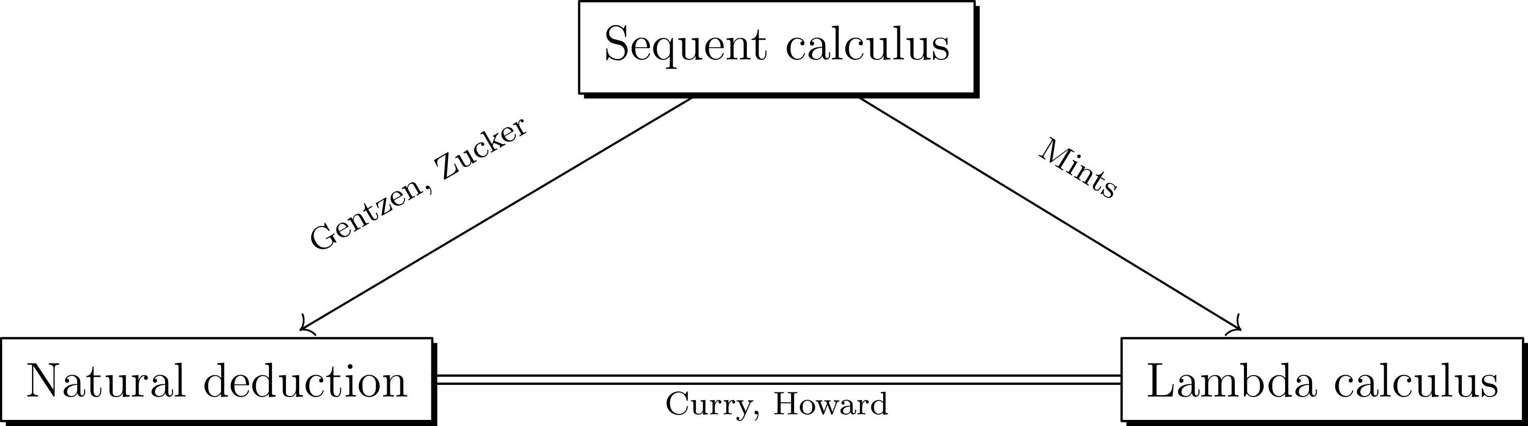
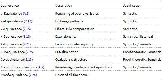

 Open access