




1 Introduction
The advent of the chirped pulse amplification (CPA) technique has led to an unprecedented development of ultra-high-power lasers[ Reference Strickland and Mourou 1 ] that have revolutionized the fields of high-density energy physics by providing new pathways to ionize and accelerate matter[ Reference Gales, Tanaka, Balabanski, Negoita, Stutman, Tesileanu, Ur, Ursescu, Andrei, Ataman, Cernaianu, D’Alessi, Dancus, Diaconescu, Djourelov, Filipescu, Ghenuche, Ghita, Matei, Seto, Zeng and Zamfir 2 , Reference Tanaka, Spohr, Balabanski, Balascuta, Capponi, Cernaianu, Cuciuc, Cucoanes, Dancus, Dhal, Diaconescu, Doria, Ghenuche, Ghita, Kisyov, Nastasa, Ong, Rotaru, Sangwan, Söderström, Stutman, Suliman, Tesileanu, Tudor, Tsoneva, Ur, Ursescu and Zamfir 3 ]. Applications range from the laser–plasma acceleration of electrons[ Reference Wan, Tata, Seemann, Levine, Kroupp and Malka 4 , Reference Aniculaesei, Ha, Yoffe, Labun, Milton, McCary, Spinks, Quevedo, Labun, Sain, Hannasch, Zgadzaj, Pagano, Franco-Altamirano, Ringuette, Gaul, Luedtke, Tiwari, Ersfeld, Brunetti, Ruhl, Ditmire, Bruce, Donovan, Downer, Jaroszynski and Hegelich 5 ], protons[ Reference Kim, Pae, Choi, Lee, Kim, Singhal, Sung, Lee, Lee, Nickles, Jeong, Kim and Nam 6 – Reference Borghesi, Fuchs, Bulanov, MacKinnon, Patel and Roth 9 ] and positrons[ Reference Spencer, Ledingham, Singhal, McCanny, McKenna, Clark, Krushelnick, Zepf, Beg, Tatarakis, Dangor, Norreys, Clarke, Allott and Ross 10 , Reference Alejo, Walczak and Sarri 11 ] to the generation of X-rays and gamma rays[ Reference Corde, Phuoc, Lambert, Fitour, Malka and Rousse 12 , Reference Ostermayr, Kreuzer, Englbrecht, Gebhard, Hartmann, Huebl, Haffa, Hilz, Parodi, Wenz, Donovan, Dyer, Gaul, Gordon, Martinez, Mccary, Spinks, Tiwari, Hegelich and Schreiber 13 ], high-order harmonics[ Reference Faenov, Magunov, Pikuz, Skobelev, Gasilov, Stagira, Calegari, Nisoli, de Silvestri, Poletto, Villoresi and Andreev 14 – Reference Edwards and Mikhailova 16 ] and nuclear reactions[ Reference Yang, McKenna, Ledingham, McCanny, Shimizu, Robson, Clarke, Neely, Norreys, Wei, Krushelnick, Nilson, Mangles and Singhal 17 , Reference Zimmer, Scheuren, Kleinschmidt, Mitura, Tebartz, Schaumann, Abel, Ebert, Hesse, Zahter, Vogel, Merle, Ahlers, Pinto, Peschke, Kröll, Bagnoud, Rodel and Roth 18 ], including fusion studies[ Reference Kline, Batha, Benedetti, Bennett, Bhandarkar, Hopkins, Biener, Biener, Bionta, Bond, Bradley, Braun, Callahan, Caggiano, Cerjan, Cagadas, Clark, Castro, Dewald, Döppner, Divol, Dylla-Spears, Eckart, Edgell, Farrell, Field, Fittinghoff, Johnson, Grim, Haan, Haines, Hamza, Hartouni, Hatarik, Henderson, Herrmann, Hinkel, Ho, Hohenberger, Hoover, Huang, Hoppe, Hurricane, Izumi, Johnson, Jones, Khan, Kozioziemski, Kong, Kroll, Kyrala, LePape, Ma, Mackinnon, MacPhee, MacLaren, Masse, McNaney, Meezan, Merrill, Milovich, Moody, Nikroo, Pak, Patel, Peterson, Piceno, Pickworth, Ralph, Rice, Robey, Ross, Rygg, Sacks, Salmonson, Sayre, Sater, Schneider, Schoff, Sepke, Seugling, Smalyuk, Spears, Stadermann, Stoeffl, Strozzi, Tipton, Thomas, Town, Volegov, Walters, Wang, Wilde, Woerner, Yeamans, Yi, Yoxall, Zylstra, Kilkenny, Landen, Hsing and Edwards 19 – Reference Norreys, Ceurvorst, Sadler, Spiers, Aboushelbaya, Mayr, Paddock, Ratan, Savin, Wang, Glize, Trines, Bingham, Hill, Sircombe, Ramsay, Allan, Hobbs, James, Skidmore, Fyrth, Luis, Floyd, Brown, Haines, Olson, Yi, Zylstra, Flippo, Bradley, Peterson, Kline and Leeper 21 ]. High-power laser facilities, such as the Extreme Light Infrastructure - Nuclear Physics (ELI-NP) facility, at the forefront with its unique 10 PW capability[ Reference Doria, Cernaianu, Ghenuche, Stutman, Tanaka, Ticos and Ur 22 – Reference Lureau, Matras, Chalus, Derycke, Morbieu, Radier, Casagrande, Laux, Ricaud, Rey, Pellegrina, Richard, Boudjemaa, Simon-Boisson, Baleanu, Banici, Gradinariu, Caldararu, De Boisdeffre, Ghenuche, Naziru, Kolliopoulos, Neagu, Dabu, Dancus and Ursescu 24 ], face the challenge of back-reflection. When solid targets are irradiated[ Reference Cernaianu, Ghenuche, Rotaru, Tudor, Chalus, Gheorghiu, Popescu, Gugiu, Balascuta, Magureanu, Tataru, Horny, Corobean, Dancus, Alincutei, Asavei, Diaconescu, Dinca, Dreghici, Ghita, Jalba, Leca, Lupu, Nastasa, Negoita, Patrascoiu, Schimbeschi, Stutman, Ticos, Ursescu, Arefiev, Tomassini, Malka, Gales, Tanaka, Ur and Doria 25 – Reference Doumy, Quéré, Gobert, Perdrix, Martin, Audebert, Gauthier, Geindre and Wittmann 27 ], part of the laser is back-reflected (BR), posing a risk to the laser system[ Reference Mishra, Andreev and Kalashinikov 28 ]. Previous research approached this issue either by performing controlled studies of the underlying phenomena[ Reference Ter-Avetisyan, Andreev, Platonov, Sung, Lee, Lee, Yoo, Singh, Ahmed, Scullion, Kakolee, Jeong, Hadjisolomou and Borghesi 29 – Reference Nistor, Magureanu and Ticos 33 ], improving the beam properties[ Reference Wittmann, Geindre, Audebert, Marjoribanks, Rousseau, Burgy, Douillet, Lefrou, Phuoc and Chambaret 34 – Reference Veetil, Schimmel, Wyrowski and Vijayan 37 ] or protecting the laser system[ Reference Dromey, Kar, Zepf and Foster 38 ]. A prevalent approach to reducing this phenomenon is the use of single or multiple plasma mirrors (PMs), which act as fast switches for back-reflection of the laser pulse and also as enhancers of the pulse ps temporal contrast[ Reference Kim, Choi, Lee, Janulewicz, Sung, Yu, Kim, Yun, Jeong and Lee 35 , Reference Dromey, Kar, Zepf and Foster 38 , Reference Kiriyama, Pirozhkov, Nishiuchi, Fukuda, Ogura, Sagisaka, Miyasaka, Mori, Sakaki, Dover, Kondo, Koga, Esirkepov, Kando and Kondo 39 ].
The study of back-reflection in PW-class laser–plasma interactions is gaining increased attention due to its significant role in the overall energy balance of laser–target interaction, as well as its importance for understanding the mechanisms responsible for enhanced laser energy absorption in plasma. This effort includes both spectral and absolute energy measurements of BR light at a 1 PW facility showing that the fraction of reflected energy is in the 1%–2% range for incident laser energy of 100–400 J on solid foils such as Cu, Al and plastic coated surfaces[
Reference Vernon, Musgrave, Green, Heathcote, Lancaster, Mendes, Hawkes and Hernandez–Gomez
40
]. Under a different set of experimental conditions, a slightly higher BR fraction (2%–4%) was measured for nanowire targets at a laser intensity of
$3\times {10}^{19}$
 W cm
${}^{-2}$
W cm
${}^{-2}$
 and a wavelength of 527 nm[
Reference Park, Tommasini, Shepherd, London, Bargsten, Hollinger, Capeluto, Shlyaptsev, Hill, Kaymak, Baumann, Pukhov, Cloyne, Costa, Hunter, Maricle, Moody and Rocca
41
]. Similar results indicating a BR coefficient of a few percent were reported for PW laser pulses focused onto micrometer- and submicrometer-thick solid foils[
Reference Ter-Avetisyan, Andreev, Platonov, Sung, Lee, Lee, Yoo, Singh, Ahmed, Scullion, Kakolee, Jeong, Hadjisolomou and Borghesi
29
]. Additional studies have examined the spectral characteristics, harmonic content (e.g., second-harmonic (SH) generation in plasma) and temporal behavior of the BR radiation[
Reference Wagner, Hornung, Schmidt, Eckhardt, Roth, Stöhlker and Bagnoud
32
,
Reference Kovács, Gilicze, Szatmáry and Földes
42
–
Reference Dua, Kant and Thakur
45
].
and a wavelength of 527 nm[
Reference Park, Tommasini, Shepherd, London, Bargsten, Hollinger, Capeluto, Shlyaptsev, Hill, Kaymak, Baumann, Pukhov, Cloyne, Costa, Hunter, Maricle, Moody and Rocca
41
]. Similar results indicating a BR coefficient of a few percent were reported for PW laser pulses focused onto micrometer- and submicrometer-thick solid foils[
Reference Ter-Avetisyan, Andreev, Platonov, Sung, Lee, Lee, Yoo, Singh, Ahmed, Scullion, Kakolee, Jeong, Hadjisolomou and Borghesi
29
]. Additional studies have examined the spectral characteristics, harmonic content (e.g., second-harmonic (SH) generation in plasma) and temporal behavior of the BR radiation[
Reference Wagner, Hornung, Schmidt, Eckhardt, Roth, Stöhlker and Bagnoud
32
,
Reference Kovács, Gilicze, Szatmáry and Földes
42
–
Reference Dua, Kant and Thakur
45
].
Here we present two new tools for the 10 PW facility dedicated to measuring the BR light from the target, which are adapted to the features of the laser system, beam transport and experimental area. The laser pulses incident on target can reach up to 240 J of energy, pulse duration of 24 fs, central wavelength
${\lambda}_{\mathrm{L}}=810$
 nm and p-polarization. The beam is focused on target in a spot with a diameter of a few micrometers by an off-axis focusing parabolic mirror (OAP) with a focal length of 1500 mm and
$F\#3$
nm and p-polarization. The beam is focused on target in a spot with a diameter of a few micrometers by an off-axis focusing parabolic mirror (OAP) with a focal length of 1500 mm and
$F\#3$
 .
.
We describe in the following the full-aperture image relay (FAIR) system followed by the small-aperture monitoring (SAM) system. We present the design and implementation of these two systems, FAIR and SAM, dedicated to the experimental area where laser pulses incident on target reach the multi-petawatt level. We outline their capabilities and limitations and present their testing and performance during commissioning experiments. A section of the high-power laser system (HPLS) together with the location of these two systems is shown in Figure 1.
Overview of the laser-experimental setup and locations of FAIR and SAM. A3.1–10 PW, preamplifier; A3.2–10 PW, main amplifier; E4, fourth optical expander in the amplification chain; E5, fifth optical expander; TB, turning box; SM, steering mirror; S, screen; FP, off-axis focusing parabola; PM, plasma mirror; T, target. Details about the full laser system including the amplifiers A1.1, A1.2 and A2 and beam expanders E1, E2 and E3 not shown here can be found in Ref. [Reference Lureau, Matras, Chalus, Derycke, Morbieu, Radier, Casagrande, Laux, Ricaud, Rey, Pellegrina, Richard, Boudjemaa, Simon-Boisson, Baleanu, Banici, Gradinariu, Caldararu, De Boisdeffre, Ghenuche, Naziru, Kolliopoulos, Neagu, Dabu, Dancus and Ursescu24] by Lureau et al.

Figure 1 Long description
A vertical schematic diagram illustrates the laser propagation path.
* At the top, the Main beam (red) enters A 3 dot 1, a 10 P W preamplifier.
* It moves down through E 4, the fourth optical expander, where a blue arrow points to a component labeled F A I R.
* The beam continues into A 3 dot 2, the 10 P W main amplifier, and then through E 5, the fifth optical expander.
* The path enters a large white block labeled 10 P W Compressor.
* Below the compressor, the beam enters the T B (turning box). Inside the T B, a steering mirror S M directs the red Main beam and a blue B R Beam. An arrow points to a small component labeled S A M.
* The beam is reflected 90 degrees to the right into the Experimental Chamber.
* Inside the chamber, the beam passes a screen S and hits an off-axis focusing parabola F P.
* A circular inset provides a close-up of the final interaction: the focused beam reflects off a plasma mirror P M and strikes the target T.
* A legend in the top right identifies the red path as the Main beam and the blue path as the B R Beam.
By combining a full-aperture approach in the laser chain and a small-aperture method at mid-distance from the target, we gain insights into the temporal, spatial, energetic and divergence characteristics of the BR light. Through this approach, we address the issue of monitoring the back-reflection in high-power laser–solid target interactions. Moreover, we correlate the measurements of these systems with a detailed estimation of the level of BR evolution in the Ti:sapphire amplifiers in order to potentially prevent any failure of optics inside the amplification chain.
2 Full-aperture image relay system
2.1 Design and implementation
The FAIR system is designed to capture the full aperture of the BR beam and analyze its features[
Reference Sharma
46
]. It was developed with our specialized ray transfer matrix analysis software, which served as the basis for both its design and implementation. At its core, FAIR is a Keplerian telescope made of two lenses L1 and L2, with focal lengths
${f}_1=800$
 mm and
${f}_2=37$
mm and
${f}_2=37$
 mm, respectively, having an input aperture with a diameter of 160 mm, as shown in Figure 2. In the laser architecture, between the desired imaging plane and FAIR, there are two beam expanders (E4 and E5) present in the optical path, as shown in Figure 1; therefore, imaging the back-reflection at specific locations over the full extent of the laser beam transport takes into account this aspect. Thus, the total magnification
$M\approx 0.027$
mm, respectively, having an input aperture with a diameter of 160 mm, as shown in Figure 2. In the laser architecture, between the desired imaging plane and FAIR, there are two beam expanders (E4 and E5) present in the optical path, as shown in Figure 1; therefore, imaging the back-reflection at specific locations over the full extent of the laser beam transport takes into account this aspect. Thus, the total magnification
$M\approx 0.027$
 is used to image an object placed at distance
${d}_{\mathrm{o}}$
is used to image an object placed at distance
${d}_{\mathrm{o}}$
 onto a charge-coupled device (CCD) found at a distance
${d}_{\mathrm{i}}$
onto a charge-coupled device (CCD) found at a distance
${d}_{\mathrm{i}}$
 , whereas the magnification of only the FAIR telescope is
${f}_2/{f}_1\approx 0.046$
, whereas the magnification of only the FAIR telescope is
${f}_2/{f}_1\approx 0.046$
 [
Reference Sharma
46
]:
[
Reference Sharma
46
]:

Design of the FAIR implemented in the laser system and ray tracing of the incoming beam (in red) traveling toward the fourth optical expander (E4) and BR beam. The transport of the BR beam shown in green is possible due to the leakage of mirror M1. SM, steering mirror; L1, L2, lenses of the imaging telescope; L3, relay lens; M2, M3, folding mirrors; BS, beam splitter; NF, near-field imaging camera; FF, far-field imaging camera.

Figure 2 Long description
The diagram illustrates an optical setup on a white surface.
* Incoming Red Beam: Enters from the top and bottom right. The bottom right section is labeled E 4 and shows the beam reflecting within a blue-outlined rectangular area. The beam travels toward the center to mirror M 1.
* Central Interaction: At M 1, the red beam is directed toward a steering mirror labeled S M on the far left.
* B R Beam Path: A green arrow indicates the B R beam originating from the leakage of mirror M 1. It travels toward S M, reflects back, and passes through M 1 toward the right side of the setup.
* Diagnostic Section: The beam, now shown in blue after passing through M 1, travels through a series of components on a gray rectangular platform.
* Component Sequence: The beam first passes through lens L 1. It then reflects off folding mirror M 2 toward folding mirror M 3.
* Imaging Path: From M 3, the beam passes through a beam splitter labeled B S. One path leads to the far-field imaging camera F F. The other path continues through lens L 2 and relay lens L 3, terminating at the near-field imaging camera N F.
Here, for example, taking as object the surface of the OAP we have
${d}_0=11927\pm 5$
 cm, and obtain
${d}_{\mathrm{i}}=8.7\pm 0.01$
cm, and obtain
${d}_{\mathrm{i}}=8.7\pm 0.01$
 cm.
cm.
The FAIR was installed inside the HPLS, between the 10 PW preamplifier (A3.1) and the main amplifier (A3.2), where the beam is 100 mm in diameter. This allows us to observe the evolution of the full-aperture BR beam close to the laser system optics. BR light is picked up from the leakage of a dielectric, high-reflectivity mirror with a transmission factor of 0.2% (M1 in Figure 2). This allows us to attenuate the beam to safe levels, for imaging it onto a CCD camera. The leakage also allows us to geometrically differentiate between the BR light and the main laser beam, which is orders of magnitude stronger; this avoids direct coupling of the main beam into the device and potentially damaging it. The FAIR was installed in a light-tight enclosure to further mitigate the significant presence of parasitic light in the HPLS. This light stems from the main pulse at 800 nm and multiple high-energy pump lasers at 532 nm. In addition, a hard-coated bandpass filter of 760–840 nm was incorporated to effectively eliminate the interference of green laser illumination by suppressing it with two orders of magnitude. These implementations benefit the operation of the FAIR greatly, but additional strategies to further suppress captured noise from the main beam would increase the device sensitivity.
The magnification factor of the system allows one to image objects as far as 120 m, by adjusting the position of the imaging CCD just a couple of millimeters away from the telescope. However, for this considerable distance, the image plane becomes virtual (i.e., the distance between L2 and the CCD is a negative value) and the extended imaging range is achieved through the integration of a third lens with focal length
${f}_3=50$
 mm, mounted in front of the near-field (NF) camera at a distance of
$2{f}_3$
mm, mounted in front of the near-field (NF) camera at a distance of
$2{f}_3$
 , thus relaying the flipped virtual image onto the CCD[
Reference Sharma
46
]. In the current configuration, the image plane is situated at
${d}_{\mathrm{i}}=-22$
, thus relaying the flipped virtual image onto the CCD[
Reference Sharma
46
]. In the current configuration, the image plane is situated at
${d}_{\mathrm{i}}=-22$
 mm, and L3 is positioned 78 mm from L2. Due to its long range, the FAIR requires a large physical footprint, which apparently makes its integration in the laser system more difficult. However, this is partially overcome by folding the telescope with two mirrors, yielding a total footprint of
$800\ \mathrm{mm}\ {\times}\ 400$
mm, and L3 is positioned 78 mm from L2. Due to its long range, the FAIR requires a large physical footprint, which apparently makes its integration in the laser system more difficult. However, this is partially overcome by folding the telescope with two mirrors, yielding a total footprint of
$800\ \mathrm{mm}\ {\times}\ 400$
 mm, as shown in Figure 2. The added benefit of this layout is the possibility of further integration of diagnostics such as an energymeter or a photodiode by swapping mirrors M2 or M3 with a leakage mirror. Between the telescope lenses, through a beam splitter (BS) with the ratio of transmission-to-reflection of 98:2, a fraction of the beam is sent to a second CCD camera (far-field, FF), provided with a sensor with 2448
$\times$
mm, as shown in Figure 2. The added benefit of this layout is the possibility of further integration of diagnostics such as an energymeter or a photodiode by swapping mirrors M2 or M3 with a leakage mirror. Between the telescope lenses, through a beam splitter (BS) with the ratio of transmission-to-reflection of 98:2, a fraction of the beam is sent to a second CCD camera (far-field, FF), provided with a sensor with 2448
$\times$
 2048 pixels and 3.45 μm pixel size[
47
]. This arrangement generates two foci, both significantly below the breakdown threshold of air, leaving the image quality unaffected: one with lower intensity on the FF CCD and a second one with higher intensity in air, transmitted through the BS. An ND1 filter was fitted to further protect the FF CCD. From the images captured by the FF camera one can infer the deviation angle of the laser beam from the optical axis with an accuracy approximately 5 μrad and its divergence with approximately 10 μrad.
2048 pixels and 3.45 μm pixel size[
47
]. This arrangement generates two foci, both significantly below the breakdown threshold of air, leaving the image quality unaffected: one with lower intensity on the FF CCD and a second one with higher intensity in air, transmitted through the BS. An ND1 filter was fitted to further protect the FF CCD. From the images captured by the FF camera one can infer the deviation angle of the laser beam from the optical axis with an accuracy approximately 5 μrad and its divergence with approximately 10 μrad.
2.2 On-site operation
During the campaign for the commissioning of the 10 PW experimental area, several BR pulses generated by the target or the PM were captured by the FAIR. The surface of the OAP shown in Figure 1 was chosen as the imaging plane. In the experiments, the high-power laser pulse was reflected from the OAP onto the PM at an incidence angle of 22.5° and then directed toward the target, as shown in Figure 1. During the gradual ramp up to full power of the laser, a remote-controlled white screen was used to shield the experimental setup from the laser beam. The screen’s front surface measured
$80\ \mathrm{cm}\,{\times}\, 80$
 cm and was made of polytetrafluoroethylene (PTFE) with 92% reflectance at 800 nm, ensuring a diffuse reflection of the incoming light.
In Figure 3 we show four instances of FAIR utilization during calibration and 10 PW shots. The transversal profile of the main beam after the compressor is shown in the first row, in Figures 3(a)–3(d). The corresponding images of back-reflection captured by the NF and FF cameras are shown in the second and third rows, respectively. In the first column of Figure 3, we show the calibration of the FAIR by sending back the central part of the attenuated laser beam (with energy of
$\sim 12$
 mJ) using a 6” mirror placed in the experimental chamber at normal incidence. This reduces both the returned energy to approximately 1.2 mJ and the beam area by a factor of 10, while maintaining the same fluence. Imaging the collimated 6” BR beam gives us an estimate of the BR beam diameter, divergence and energy on the FAIR. By placing various patterns of sharp-edged objects in the object plane (i.e., in front of the 6” mirror) we further fine-tuned the image plane by adjusting the position of the NF CCD. This physical calibration of the FAIR performed with the attenuated beam of the HPLS matches with our model generated by the ray analysis software. Moreover, it was determined that the FAIR can perceive distance deviations of approximately 0.5 m from the object plane. The fluence of the BR beam captured in Figure 3(a1) during FAIR calibration with the 12 mJ incoming beam is approximately
$4\times {10}^{-5}$
mJ) using a 6” mirror placed in the experimental chamber at normal incidence. This reduces both the returned energy to approximately 1.2 mJ and the beam area by a factor of 10, while maintaining the same fluence. Imaging the collimated 6” BR beam gives us an estimate of the BR beam diameter, divergence and energy on the FAIR. By placing various patterns of sharp-edged objects in the object plane (i.e., in front of the 6” mirror) we further fine-tuned the image plane by adjusting the position of the NF CCD. This physical calibration of the FAIR performed with the attenuated beam of the HPLS matches with our model generated by the ray analysis software. Moreover, it was determined that the FAIR can perceive distance deviations of approximately 0.5 m from the object plane. The fluence of the BR beam captured in Figure 3(a1) during FAIR calibration with the 12 mJ incoming beam is approximately
$4\times {10}^{-5}$
 J cm
${}^{-2}$
J cm
${}^{-2}$
 (accounting for losses). Most BR traces captured from multi-PW shots are larger in diameter but roughly within the same fluence range. We conclude that the BR beam reaching the HPLS is within the millijoule to tens of millijoules range. The sensitivity of the device was estimated to be approximately
$2.1\times {10}^{-5}$
(accounting for losses). Most BR traces captured from multi-PW shots are larger in diameter but roughly within the same fluence range. We conclude that the BR beam reaching the HPLS is within the millijoule to tens of millijoules range. The sensitivity of the device was estimated to be approximately
$2.1\times {10}^{-5}$
 J cm
${}^{-2}$
J cm
${}^{-2}$
 (or 40 mJ for the full 50 cm beam). This is mostly limited by the captured noise, which stems from the sum of all scattering generated by the main beam across dozens of optical components from the laser bay. Utilizing the HPLS beam, the position of the FF CCD was fine-tuned for best focus; this is presented in Figure 3(a2).
False-color images. (a) Beam profile of the approximately 12 mJ pulse sent to the 6” mirror: (a1) NF of the 6” BR beam; (a2) FF of the 6” BR beam. (b) Beam profile of the 10 PW full power shot sent onto a diffusive white screen: (b1) corresponding response of the NF camera with no image from the screen; (b2) corresponding capture by the FF camera with no signal. (c) Main beam profile of the 10 PW pulse sent on target via a PM: (c1) corresponding image of the BR beam caught on the NF camera during a shot on target with a PM; (c2) corresponding image of the shot on target captured on the FF camera; the image is doubled by the two-surface reflection of the BS located in the FAIR, which splits the beam for the NF and FF. (d) Main beam profile of the 10 PW pulse sent to the PM (no target): (d1) corresponding image of back-reflection captured by the NF camera from a shot on the PM; (d2) corresponding image of back-reflection caught by the FF camera.

Figure 3 Long description
The grid consists of four columns labeled a, b, c, and d, each containing three vertical panels.
* Column a: Top panel a shows a circular, textured green and blue beam profile. Middle panel a 1 shows a smaller, bright green circular spot with a 10 cm scale bar. Bottom panel a 2 shows two tiny, faint green points on a dark purple background.
* Column b: Top panel b shows a bright yellow-green circular beam profile with high intensity. Middle panel b 1 and bottom panel b 2 are both uniform dark blue and purple squares with no visible signal or features.
* Column c: Top panel c shows a bright yellow-green circular beam profile similar to b. Middle panel c 1 shows a faint, broken ring of light along the perimeter of a circular area. Bottom panel c 2 shows two overlapping, faint green crescent shapes at the center.
* Column d: Top panel d shows a bright yellow-green circular beam profile. Middle panel d 1 shows a very large, saturated yellow circular spot with fuzzy edges. Bottom panel d 2 shows a medium-sized, soft-edged green circular glow.
All panels use a false-color heat map where purple represents low intensity and yellow represents high intensity.
Figure 3(b) shows the incoming full power shot sent to the PTFE diffusing screen inserted in the laser path. This is most likely due to the screen’s ability to effectively scatter uniformly the half-solid angle, so that not much light will reach HPLS. Moreover, the distance between the experimental area and the FAIR is approximately 120 m, which further reduces the amount of light reaching the device. This situation is shown in Figures 3(b1) and 3(b2) where the FAIR NF and FF CCDs do not capture images. In the third instance, Figure 3(c), the laser beam is directed to the target via the PM. We can clearly see in Figure 3(c1) the spatial profile of back-reflection for the full beam aperture given by the NF camera. It shows a highly nonuniform transversal profile in the shape of a ring with diameter 689
$\pm$
 9 mm, being 40% larger than the main laser beam diameter. This corresponds to a half-angle divergence of the BR beam
$\theta \approx 3.4\times {10}^{-3}$
9 mm, being 40% larger than the main laser beam diameter. This corresponds to a half-angle divergence of the BR beam
$\theta \approx 3.4\times {10}^{-3}$
 rad at the location of the FAIR.
Due to the spatial intensity gradient of the multi-PW beam from its edge toward the center, the triggering process (specifically, the ablation of the PM) is nonuniform. In Figure 4(a), we present an intensity map generated from the main beam profile projected on the PTFE screen in the interaction chamber. Here, we observe that the top-hat beam has slight intensity modulations, and notably a ramp-up (or transition) region from the edges toward the center, highlighted in blue. When reaching the PM, at the edge of the triggered zone, a ring-like area is generated where the anti-reflection (AR) coating has been fully removed by the low laser intensity of the transition region, exposing a clean BK7 glass surface. Further toward the center, the rapidly increasing intensity destroys both the AR coating and the polished BK7 surface, resulting in a darkened, frosted and slightly opaque burn mark. Thus, the interaction between the multi-PW beam and the PM creates a relatively high-reflectivity ring-shaped region. This reflectivity variation of the utilized PM will imprint spatial intensity modulation favoring the formation of a ring-shaped profile to any subsequent reflected beam (i.e., the back-reflection stemming from the target). To validate this mechanism, we performed a reflectivity test utilizing an already used PM slab and a fiber laser (
$\approx$
 500 mW and 800 nm wavelength) to simulate the experimental geometry (i.e., maintaining the same polarization, wavelength and incidence angle). For this test, the alignment beam was polarized and expanded to encompass the damaged surface of the PM (
$\approx$
500 mW and 800 nm wavelength) to simulate the experimental geometry (i.e., maintaining the same polarization, wavelength and incidence angle). For this test, the alignment beam was polarized and expanded to encompass the damaged surface of the PM (
$\approx$
 30 mm). The reflected profile presented in Figure 4(b) was captured on a white screen approximately equal to 1.5 m from PM, enough to spatially separate the second surface reflection.
(a) Three-dimensional (3D) map of the intensity distribution across the main beam spatial profile. (b) Obtained spatial distribution in the PM reflectance test. Note, the lower full beam is the second surface reflection.

Figure 4 Long description
Panel a. A 3 D surface plot representing intensity distribution. The base of the beam profile is a dark blue oval on a white grid. A red arrow points to this blue perimeter with the text Transition region highlighted in blue. Moving upward, the intensity increases into a large, jagged plateau colored in magenta and pink, featuring numerous sharp peaks. The grid axes are labeled with values 279.0 and 213.0.
Panel b. A vertical spatial distribution against a black background. At the top is a bright magenta ring-shaped beam with a small central dot. Directly below it and touching the first ring is a second, slightly larger and more diffused magenta circular reflection. This lower feature represents the second surface reflection in the P M reflectance test.
By comparing the ring structures shown in Figures 3(c1) and 4(b), we can assert that the emergence of ring-shaped BR profiles captured across all multi-PW shots with various target types is the product of the damaged PM with the variable reflectivity imprinted by the multi-PW beam.
In Figure 3(c2) the corresponding FF image shows a beam with half-angle divergence of
$\theta \approx 2.9\times {10}^{-3}$
 rad, which is in good agreement with the value calculated above for the image shown in Figure 3(c1). According to the divergence captured by the FAIR, we can back-track and infer the initial beam divergence stemming from the target prior to interaction with expanders E5 and E4. This is possible due to a relationship between the divergence and beam diameter in optical formalism[
Reference Pedrotti, Pedrotti and Pedrotti
48
], as presented in Equation (2). For the back-reflection, we estimate
${\theta}_{\mathrm{out}}\approx 1.6\times {10}^{-3}$
rad, which is in good agreement with the value calculated above for the image shown in Figure 3(c1). According to the divergence captured by the FAIR, we can back-track and infer the initial beam divergence stemming from the target prior to interaction with expanders E5 and E4. This is possible due to a relationship between the divergence and beam diameter in optical formalism[
Reference Pedrotti, Pedrotti and Pedrotti
48
], as presented in Equation (2). For the back-reflection, we estimate
${\theta}_{\mathrm{out}}\approx 1.6\times {10}^{-3}$
 rad in A3.2 and
${\theta}_{\mathrm{in}}\approx 0.5\times {10}^{-3}$
rad in A3.2 and
${\theta}_{\mathrm{in}}\approx 0.5\times {10}^{-3}$
 rad in vacuum transport tubes, with
${M}_{\mathrm{E}5}\approx 0.3$
rad in vacuum transport tubes, with
${M}_{\mathrm{E}5}\approx 0.3$
 being the magnification of the expander[
Reference Pedrotti, Pedrotti and Pedrotti
48
]:
being the magnification of the expander[
Reference Pedrotti, Pedrotti and Pedrotti
48
]:

In Figure 3(d) we present an outstanding case, where a multi-PW shot was delivered on the PM (i.e., without target) during a PM reflectance test. Here, the diameter of the beam on the PM was measured to be around 3 mm with an irradiance that exceeded
${10}^{17}$
 W cm
${}^{-2}$
W cm
${}^{-2}$
 (unlike the common configuration of 20 mm diameter with a corresponding irradiance of the order of magnitude of
${10}^{15}$
(unlike the common configuration of 20 mm diameter with a corresponding irradiance of the order of magnitude of
${10}^{15}$
 W cm
${}^{-2}$
W cm
${}^{-2}$
 ). Note the homogeneous spatial profile in Figure 3(d1) and slightly lower divergence inferred from Figure 3(d2) than in the previous case because the PM is acting as a target. These intricate findings will be further investigated in-depth in future experiments when statistics based on a large number of shots on different types of target can be built.
3 Small-aperture monitoring system
3.1 Design and implementation
In the second optical system, we utilized a setup based on a fast photodiode and an optical fiber coupled to an optical spectrometer to detect and record the BR light. The large steering mirror (SM) located within the turning box (TB), in vacuum, has a dielectric front surface coating and a frosted back surface. Its purpose is to direct the main laser beam toward the experimental area, as shown in detail in Figure 5. Within the TB, three identical dielectric mirrors are positioned in a configuration that collects the central part of the BR beam through the leakage of the large SM. These mirrors are 6” in diameter with coating optimized for reflection in the range of 760–850 nm. We expect this beam to be significantly attenuated by several orders of magnitude due to the low transmission through the layers of the SM. From the positioning of the mirrors, similarly to the FAIR, this setup allows for spatial differentiation between the incoming and BR beams. The collected BR beam is sent outside the TB through a viewport, a DN160, with the diameter of the window of 150 mm. It is subsequently focused onto a fast photodiode using a 2” lens with focal length of 150 mm. Data acquisition is done on a 1 GHz oscilloscope with 10 GS/s maximum sampling rate.
(a) Top view of the SAM setup inside the turning box (TB). (b) Graphical representation of the TB containing the large SM and the optical assembly of SAM. The electromagnetic pulse shielded photodiode is shown in black.

Figure 5 Long description
Panel a is a top-down photograph of the interior of a metallic turning box containing the S A M setup. It shows various mounting brackets, wires, and a large angled metallic assembly.
Panel b is a 3 D schematic diagram of the optical assembly. A legend at the bottom right identifies a red arrow as the Incoming Beam and a green arrow as the B R Beam.
Path of light:
* The red Incoming Beam enters from the bottom, reflects off a large teal Steering Mirror at a 90-degree angle, and exits to the left.
* An Optical Fiber is located in the center-right of the box.
* The blue B R Beam path is marked by green arrows and numbered mirrors 1, 2, and 3.
* The beam travels from the fiber to mirror 3 (bottom right), reflects to mirror 2 (top right), then to mirror 1 (top left).
* From mirror 1, the blue beam travels downward, passing through the red beam path.
* At the bottom left, the blue beam passes through a Lens and terminates at a black cube labeled Photodiode.
SAM records temporal signals that have a total length of approximately 150 ns, using a fast photodiode produced by Newport Corp., model 818-BB-21, which features a 300 ps rise time[ 49 ]. It allows the detection of both the trace of the 10 PW and BR pulses given that the time delay between them is approximately 120 ns. The relatively high temporal resolution can potentially yield the ns contrast of the BR pulse and can give clues about the possible optical pathways of the light from the target to the detector. In other words, the time delay between BR peaks together with their relative intensities can be correlated with a ray-tracing simulation to obtain information about the divergence and timing of the BR beam. Such information could potentially offer insights into the time evolution of the laser–plasma interaction processes.
Furthermore, the employed photodiode was calibrated in terms of incident energy using the main laser, which delivered pulses at controlled low energy. It was estimated that laser pulses with 20 mJ energy starting off in the laser bay arriving in the experimental area attenuated down to approximately 11.7 mJ. Here, a metal-coated mirror with 6” in diameter back reflected the laser beam. The mirror was positioned with the surface normal to the laser beam propagation direction and its center aligned with the axis of the BR system. This would allow the direct determination of the incident BR pulse energy.
The energy losses and their coefficients incurred during the detection of BR light in our system were as follows: reflection
${R}_{\mathrm{metal}}$
 on the 6” metallic mirror, transmission
${T}_{\mathrm{SM}}$
on the 6” metallic mirror, transmission
${T}_{\mathrm{SM}}$
 of the large SM, fraction
$S$
of the large SM, fraction
$S$
 of the pickoff beam area relative to that of the main laser beam with diameter 50 cm, total reflection coefficient of the three pickoff mirrors
${R}_{\mathrm{m}}$
of the pickoff beam area relative to that of the main laser beam with diameter 50 cm, total reflection coefficient of the three pickoff mirrors
${R}_{\mathrm{m}}$
 inside the TB, transmission
${T}_{\mathrm{VP}}$
inside the TB, transmission
${T}_{\mathrm{VP}}$
 of the viewport, transmission
${T}_{\mathrm{l}}$
of the viewport, transmission
${T}_{\mathrm{l}}$
 of the focusing lens and transmission of the bandpass filter
${T}_{\mathrm{f}}$
of the focusing lens and transmission of the bandpass filter
${T}_{\mathrm{f}}$
 . Thus, the energy detected by our system during calibration was
${E}_{\mathrm{BR}}^{\mathrm{cal}}={E}_0\cdot {F}_{\mathrm{cal}}$
. Thus, the energy detected by our system during calibration was
${E}_{\mathrm{BR}}^{\mathrm{cal}}={E}_0\cdot {F}_{\mathrm{cal}}$
 , where
${E}_0=11.7$
, where
${E}_0=11.7$
 mJ and
${F}_{\mathrm{cal}}={R}_{\mathrm{metal}}\cdot {T}_{\mathrm{SM}}\cdot S\cdot {R}_{\mathrm{m}}\cdot {T}_{\mathrm{VP}}\cdot {T}_{\mathrm{l}}\cdot {T}_{\mathrm{f}}$
mJ and
${F}_{\mathrm{cal}}={R}_{\mathrm{metal}}\cdot {T}_{\mathrm{SM}}\cdot S\cdot {R}_{\mathrm{m}}\cdot {T}_{\mathrm{VP}}\cdot {T}_{\mathrm{l}}\cdot {T}_{\mathrm{f}}$
 .
.
A careful assessment of
${T}_{\mathrm{SM}}$
 was carried out by utilizing a laser diode emitting at 800 nm. Its beam was sent through the SM incident at 45°, which is the operating angle of the mirror; the power of the transmitted beam was measured with a sensitive powermeter, along the propagation direction. As expected, the measured value
${{T}_{\mathrm{SM}}=(6.83\pm 0.05)\times {10}^{-5}}$
was carried out by utilizing a laser diode emitting at 800 nm. Its beam was sent through the SM incident at 45°, which is the operating angle of the mirror; the power of the transmitted beam was measured with a sensitive powermeter, along the propagation direction. As expected, the measured value
${{T}_{\mathrm{SM}}=(6.83\pm 0.05)\times {10}^{-5}}$
 was low, given that the SM has a high reflectivity in the bandwidth of the HPLS centered at 800 nm. For the other factors we have
${R}_{\mathrm{metal}}=0.98$
was low, given that the SM has a high reflectivity in the bandwidth of the HPLS centered at 800 nm. For the other factors we have
${R}_{\mathrm{metal}}=0.98$
 ,
$S=1.032\times {10}^{-2}$
,
$S=1.032\times {10}^{-2}$
 ,
${{R}_{\mathrm{m}}=0.97}$
,
${{R}_{\mathrm{m}}=0.97}$
 ,
${T}_{\mathrm{VP}}=0.9$
,
${T}_{\mathrm{VP}}=0.9$
 ,
${T}_{\mathrm{l}}=0.9$
,
${T}_{\mathrm{l}}=0.9$
 and
${T}_{\mathrm{f}}=0.976$
and
${T}_{\mathrm{f}}=0.976$
 . This gives a calibration factor
${F}_{\mathrm{cal}}\approx 5.4\times {10}^{-7}$
. This gives a calibration factor
${F}_{\mathrm{cal}}\approx 5.4\times {10}^{-7}$
 and an incident energy on the detector
${E}_{\mathrm{BR}}^{\mathrm{cal}}\approx 6.2$
and an incident energy on the detector
${E}_{\mathrm{BR}}^{\mathrm{cal}}\approx 6.2$
 nJ. The signal produced by the photodiode on the oscilloscope had a peak value of 125 mV. A correspondence in units of incident energy can be quickly established in our BR system for the detected signal, considering a linear response of the photodetector in a range where it is not saturated[
49
]: 5 nJ/100 mV. Note that this value of incident beam energy on the detector is an absolute calibration value and will be used in the following to estimate the BR energy for laser shots on targets. This calibration can be extended to a one-to-one equivalence between the BR energy and the measured signal. For this particular arrangement, which includes the 6” metallic mirror in the setup, the calibration factor is approximately 9.4 mJ to
$100$
nJ. The signal produced by the photodiode on the oscilloscope had a peak value of 125 mV. A correspondence in units of incident energy can be quickly established in our BR system for the detected signal, considering a linear response of the photodetector in a range where it is not saturated[
49
]: 5 nJ/100 mV. Note that this value of incident beam energy on the detector is an absolute calibration value and will be used in the following to estimate the BR energy for laser shots on targets. This calibration can be extended to a one-to-one equivalence between the BR energy and the measured signal. For this particular arrangement, which includes the 6” metallic mirror in the setup, the calibration factor is approximately 9.4 mJ to
$100$
 mV peak signal on the scope. In the current configuration we can discern BR traces of around 4 mV, which corresponds to approximately 1.5 mJ; this is three orders more sensitive than what the HPLS can theoretically handle in terms of BR energy. If other optical components are inserted into the path of the BR beam, then the attenuation factor
$F$
mV peak signal on the scope. In the current configuration we can discern BR traces of around 4 mV, which corresponds to approximately 1.5 mJ; this is three orders more sensitive than what the HPLS can theoretically handle in terms of BR energy. If other optical components are inserted into the path of the BR beam, then the attenuation factor
$F$
 will change.
In our experiments, additional attenuation was further introduced by the insertion of a neutral density filter, an ND0.6, to maintain the captured signal within the linear response of the photodiode. As such, the captured signal has to be multiplied by the attenuation factor of this filter
${T}_{\mathrm{ND}}=0.25$
 . Also, the reflection coefficient of the ablated surface of the PM
${R}_{\mathrm{PM}}$
. Also, the reflection coefficient of the ablated surface of the PM
${R}_{\mathrm{PM}}$
 and that of the OAP,
${R}_{\mathrm{OAP}}$
and that of the OAP,
${R}_{\mathrm{OAP}}$
 , must be included in the calculations. We found that
${R}_{\mathrm{PM}}\ \mathrm{was\ approximately}\ 0.05$
, must be included in the calculations. We found that
${R}_{\mathrm{PM}}\ \mathrm{was\ approximately}\ 0.05$
 on the damaged surface of the AR coating of the PM using laser light at 800 nm. We also measured the reflectance of the PM on its intact surface and found a lower value of approximately 0.03. Here,
${R}_{\mathrm{OAP}}=0.998$
on the damaged surface of the AR coating of the PM using laser light at 800 nm. We also measured the reflectance of the PM on its intact surface and found a lower value of approximately 0.03. Here,
${R}_{\mathrm{OAP}}=0.998$
 as provided by the manufacturer. Thus, the total attenuation factor is
${F}_{\mathrm{exp}}\approx 6.65\times {10}^{-9}$
as provided by the manufacturer. Thus, the total attenuation factor is
${F}_{\mathrm{exp}}\approx 6.65\times {10}^{-9}$
 , where
${F}_{\mathrm{exp}}={R}_{\mathrm{PM}}\cdot {R}_{\mathrm{OAP}}\cdot {T}_{\mathrm{SM}}\cdot S\cdot {R}_{\mathrm{m}}\cdot {T}_{\mathrm{VP}}\cdot {T}_{\mathrm{l}}\cdot {T}_{\mathrm{f}}\cdot {T}_{\mathrm{ND}}$
, where
${F}_{\mathrm{exp}}={R}_{\mathrm{PM}}\cdot {R}_{\mathrm{OAP}}\cdot {T}_{\mathrm{SM}}\cdot S\cdot {R}_{\mathrm{m}}\cdot {T}_{\mathrm{VP}}\cdot {T}_{\mathrm{l}}\cdot {T}_{\mathrm{f}}\cdot {T}_{\mathrm{ND}}$
 . From the above calibration factor
${F}_{\mathrm{exp}}$
. From the above calibration factor
${F}_{\mathrm{exp}}$
 we can infer the scaling of the BR energy at the target surface is approximately 0.75 J for a measured peak of 100 mV on our detector. Note that the transmitted light to our measuring setup is initially reflected by the damaged PM and then by the focusing parabola. We end up with the absolute value of BR energy: 39 mJ/100 mV detected signal. Furthermore, when assessing the effective BR energy that goes into the last amplifier A3.2 of the laser chain we should account for the reflection on the SM (
$\sim 0.998$
we can infer the scaling of the BR energy at the target surface is approximately 0.75 J for a measured peak of 100 mV on our detector. Note that the transmitted light to our measuring setup is initially reflected by the damaged PM and then by the focusing parabola. We end up with the absolute value of BR energy: 39 mJ/100 mV detected signal. Furthermore, when assessing the effective BR energy that goes into the last amplifier A3.2 of the laser chain we should account for the reflection on the SM (
$\sim 0.998$
 ) and the transmission of the compressor (
$\sim 0.735$
) and the transmission of the compressor (
$\sim 0.735$
 ), which leads to approximately 29 mJ per 100 mV peak signal on our photodiode. During laser shots on targets in the setup configuration discussed above we typically measured a BR signal with peak values of approximately 100–500 mV, depending on the type of target. This means that the real BR energy returning into the laser ranges from a few tens of mJ up to approximately 140 mJ, which is in good agreement with the values captured by the FAIR. Based on the measured PM reflectivity,
${R}_{\mathrm{PM}}\sim 0.05$
), which leads to approximately 29 mJ per 100 mV peak signal on our photodiode. During laser shots on targets in the setup configuration discussed above we typically measured a BR signal with peak values of approximately 100–500 mV, depending on the type of target. This means that the real BR energy returning into the laser ranges from a few tens of mJ up to approximately 140 mJ, which is in good agreement with the values captured by the FAIR. Based on the measured PM reflectivity,
${R}_{\mathrm{PM}}\sim 0.05$
 , we can infer that its absence in the experimental setup could have potentially boosted the back-reflection to
$1$
, we can infer that its absence in the experimental setup could have potentially boosted the back-reflection to
$1$
 J.
J.
Besides the SM, an optical assessment of the three 6” mirrors was also performed. These assessments revealed that the photodiode is susceptible to detecting wavelengths beyond the bandwidth centered around 800 nm, which can originate from interactions within the experimental chamber. While the three dielectric mirrors exhibit high reflectivity at 800 nm, they are still capable of steering visible and ultraviolet (UV) components toward the photodiode. Considering the combined contributions from the SM and TB mirrors, and assuming a 1 J input pulse from the interaction chamber, the following energies were estimated to reach the photodiode: 69.4 μJ at 532 nm, 2.5 μJ at 635 nm and 66.3 μJ at 800 nm. For the purpose of machine safety, only the infrared (IR) components of the beam are of interest, because the optical compressor and the subsequent dielectric optics in the system will rapidly filter out other spectral components. To mitigate these spectral contributions, a bandpass filter (735–900 nm) has been installed in front of the photodiode.
3.2 On-site operation
In Figure 6 two shots delivered on screen and target with their respective BR trace captured by SAM are shown. In both cases, the 10 PW laser pulse generates a directly scattered component from the SM, accompanied by artifacts resulting from parasitic scattering processes inside the TB. The BR signal is seen delayed in time with roughly 98.8 and 114.5 ns from the screen and target, respectively. This corresponds to a distance traveled by light to the screen and target of 29.6 and 34.3 m, respectively. These distances correlate well with the physical lengths measured inside the experimental area: 29.75
$\pm$
 0.1 and 35.15
$\pm$
0.1 and 35.15
$\pm$
 0.1 m.
Captured trace of the 10 PW laser pulse together with BR light in two separate laser shots: on a white screen and on a thin Al foil target with three thicknesses with a PM at 10 PW.

Figure 6 Long description
A line graph plots Photodiode Voltage in Volts on the y-axis from 0.0 to 1.6 against Time in n s on the x-axis from 0 to 120. Two data lines are shown: an orange trace and a blue trace.
Moving from left to right along the x-axis:
* At 0 n s, a small peak in the orange trace reaching approximately 0.1 V is labeled Main pulse.
* Between 5 and 25 n s, a large multi-peaked signal in the orange trace reaching nearly 0.9 V is enclosed in a blue box and labeled Parasitic scattering from the main pulse.
* Between 95 and 110 n s, a very high double-peak in the orange trace reaching 1.55 V and 1.1 V is enclosed in a blue box and labeled B R from the screen.
* At approximately 115 n s, a small sharp peak in the blue trace reaching 0.2 V is enclosed in a small blue box and labeled B R from target.
The baseline for both traces remains near 0.0 V between the identified signal clusters.
The aforementioned artifacts of the main pulse are produced by the scattering induced while traveling through the vacuum transport system and interacting with optical components, such as gratings and mirrors. As such, this strong illumination easily couples into the detector from several directions, which corresponds to the peaks seen in Figure 7(b). The main pulse trace shown in Figure 7(a) is barely visible in contrast with the artifacts, as it is highly collimated and aimed toward the target. Initially, it was presumed that the structures observed in Figures 7(a) and 7(b) represent a strong prepulse followed by the main laser pulse. Later it was confirmed that there is no nanosecond prepulse of this intensity. The optical path of light representing the peak in Figure 7(a) is from the SM surface to the viewport and then to the detection system. The first peak in Figure 7(b) (No. 1) is scattered light from the SM, collected by the 6” mirror positioned in-line with the viewport (denoted No. 1 in Figure 7(b)). The highest peak (No. 2) comes from the light collected by the mirror placed in the corner of the TB, which has a direct view of the back of the SM (No. 2 in Figure 7(b)). Finally, the last peak (No. 3) is from light collected by the mirror positioned close to the rear-side of the SM (No. 3 in Figure 7(b)).
Data from 20 laser shots (with power varying in the range of 8–10 PW) delivered to the experimental area on targets and a white screen: (a) trace of the main incident laser pulse; (b) parasitic scattering from the main pulse with the peaks corresponding to the dielectric mirrors; (c) back-reflection from the screen; (d) back-reflection from the target.

Figure 7 Long description
The graph plots Photodiode Voltage in V on the y-axis from 0.0 to 1.4 against Time in n s on the x-axis. The x-axis is split into two segments: -5 to 40 n s and 95 to 130 n s. Vertical black lines separate the four panels.
* Panel a: Shows a small initial pulse at 0 n s.
* Panel b: Contains three distinct peaks. Peak 1 is at approximately 9 n s (0.75 V), Peak 2 is the highest in this section at 11 n s (1.05 V), and Peak 3 is at 17 n s (0.5 V).
* Panel c: Displays a high-intensity region. Peak 4 is the maximum voltage at 97 n s (1.45 V). Blue arrows point to Peak 5 (a shoulder on the decline of Peak 4), Peak 6 (a sharp rise at 105 n s reaching 1.1 V), and Peak 7 (a small bump at 111 n s).
* Panel d: Shows the final reflections. Peak 8 is a sharp spike at 114 n s (1.1 V). A blue arrow points to Peak 9, which is a secondary shoulder at 116 n s. Peak 10 is a final smaller spike at 122 n s (0.35 V).
The data represents 20 overlaid laser shots, showing high consistency in the timing and amplitude of the peaks.
The BR trace obtained from the white screen seen in Figure 7(c) has a particular temporal structure with four peak regions, present in all recorded shots. The PTFE screen acts as a quasi-Lambertian diffuser, thus scattering the light almost uniformly over the entire half-solid angle. We identified that from all the scattered light the four clearly defined peaks match with four geometrical paths with distinct lengths of the scattered light on its way to the detector. By analyzing the geometry of the vacuum transport system, we determined that the scattered light from the screen that is reaching directly the SM via the shortest path is responsible for the first peak, as it is capable of strongly illuminating the TB. This peak encompasses the next one during its slow fall-off (Nos. 4 and 5 in Figure 7). This structure is expected when a quasi-scattered light reaches the detector. Peak No. 6, shown in Figure 7, is delayed to No. 4 by the loop of the BR setup, which has an optical path of
$3.98\pm 0.09$
 m. Signal No. 6 starts with a sharp increase and is followed by a slow fall-off that morphs into peak No. 7. This is a large portion of the scattered light from the screen coupling into the vacuum tube, which directs it toward the TB and strongly illuminates it; strong scattering is consistent with a longer signal on the photodiode.
Analyzing the signal from the shots on target, shown in Figure 7(d), we observe that the recorded peak is actually composed of two close features: one at 114 ns (No. 8), and a second, smaller one, at 116 ns (No. 9). This corresponds to a distance of approximately 30 cm, which aligns well with the location of the telescope assembly located behind the target. The telescope is utilized for target and beam alignment. In subsequent experimental campaigns, another peak (No. 10) appeared, located at approximately 122 ns. This corresponds to a reflection stemming from the interaction chamber, located at a physical distance of 1.2 m behind the target, accounting for the round-trip duration.
To characterize the BR spectrum, SAM was fitted with an optical fiber that coupled the light from behind the large SM to a broadband spectrometer, using a 1” collimator. This allowed capturing of BR spectra[
Reference Vernon, Musgrave, Green, Heathcote, Lancaster, Mendes, Hawkes and Hernandez–Gomez
40
] from multi-petawatt shots delivered both on target, as shown in Figure 8, and the aforementioned outstanding case of the standalone PM, shown in Figure 9. In spite of the low transmission coefficient of the SM, the relatively small collection area of the fiber and reduced reflection off the deteriorated PM (with coefficient
${R}_{\mathrm{PM}}\sim 0.05$
 ), the captured signal with the spectrometer is solid. This indicates that the generated level of back-reflection in the spectral range is high, as shown in Figures 8 and 9. The first observation is that the interaction of ultra-short pulses with the target via the PM generates the SHs[
Reference Dua, Kant and Thakur
45
,
Reference Kaur, Agarwal and Kaur
50
]. Here,
$2{\omega}_{\mathrm{L}}$
), the captured signal with the spectrometer is solid. This indicates that the generated level of back-reflection in the spectral range is high, as shown in Figures 8 and 9. The first observation is that the interaction of ultra-short pulses with the target via the PM generates the SHs[
Reference Dua, Kant and Thakur
45
,
Reference Kaur, Agarwal and Kaur
50
]. Here,
$2{\omega}_{\mathrm{L}}$
 peaks at 405 nm, which is scattered back into the laser system. A strong line emerges at 725 nm only for one shot, accompanied by a low peak at 690 nm. For all other shots there is a low-intensity peak at 635 nm. Apparently there is no clear correlation between the signal strength and target thickness; the target thickness spans between a few hundred nanometers and micrometers, as shown in Figure 8. In all these shots the footprint on the PM was kept constant. The target made of ultrathin Au (150 nm) yielded the highest signal, followed by Al (400 nm) and Au (1.3 μm). These results need further investigation during the full commissioning of this experimental area.
Captured BR spectra during experiments with different targets and a PM inserted in the optical path, with the respective intensities achieved on target. The thickness and material are indicated for each target. The intensity on the PM is approximately
${10}^{15}$
 W cm
${}^{-2}$
W cm
${}^{-2}$
 .
.

Figure 8 Long description
The line graph plots Counts on the vertical Y-axis, ranging from 0 to 800, against Wavelength in n m on the horizontal X-axis, ranging from 350 to 1050.
Six datasets are shown, each representing a different target material and thickness.
* All datasets exhibit a primary cluster of peaks between 400 and 430 n m. The highest peak in this region reaches approximately 600 counts for the A u 150 n m target (red line).
* A secondary, smaller peak occurs for most targets near 630 n m, reaching roughly 100 to 150 counts.
* A distinct, sharp peak unique to the A u 150 n m target (red line) appears at approximately 725 n m, reaching 600 counts.
* Beyond 750 n m, all lines flatten into low-intensity noise near the 0 count baseline.
The legend in the top right identifies the targets and their intensities in W cm super -2.
* N i 1 mu m at 4.9 dot 10 super 22 (blue).
* A l 400 n m at 4.9 dot 10 super 22 (orange).
* A l 400 n m at 4.9 dot 10 super 22 (green).
* A u 150 n m at 4.8 dot 10 super 22 (red).
* A u 1.3 mu m at 4.8 dot 10 super 22 (purple).
* A u 10 n m at 4.6 dot 10 super 22 (brown).
Captured BR spectra exclusively from PM with laser intensity in the range of
${10}^{16}$
 –
${10}^{17}$
–
${10}^{17}$
 W/cm
${}^2$
W/cm
${}^2$
 and the spectral-dependent reflectivity of the steering mirror (
${R}_{\mathrm{SM}}$
and the spectral-dependent reflectivity of the steering mirror (
${R}_{\mathrm{SM}}$
 ).
).

Figure 9 Long description
The x-axis represents Wavelength in n m, ranging from 350 to 1050. The left y-axis represents Counts from 0 to 800. The right y-axis represents R sub S M in percent from 0 to 100.
Three spectral datasets are plotted:
* Blue line (2.7 times 10 super 16 W dot cm super minus 2): Shows a single sharp peak near 400 n m reaching approximately 550 counts, then remains at baseline.
* Orange line (3.7 times 10 super 16 W dot cm super minus 2): Shows a sharp peak near 415 n m reaching approximately 650 counts, then remains at baseline.
* Green line (1.2 times 10 super 17 W dot cm super minus 2): Displays a broad plateau between 400 and 450 n m at 600 counts, followed by numerous smaller oscillating peaks across the 500 to 750 n m range, and a final set of low-intensity peaks between 900 and 1050 n m.
A fourth red line represents the steering mirror reflectivity (R sub S M). It remains at 0 percent until 720 n m, rises sharply to a plateau of nearly 100 percent between 750 and 880 n m, and then drops sharply back to 0 percent by 900 n m.
To better understand the results, several shots were taken solely on the PM, with no target placed in the focus of the laser beam, while slowly reducing the footprint on the PM, which led to an increase in the intensity up to 10
${}^{17}$
 W cm
${}^{-2}$
W cm
${}^{-2}$
 , as shown in Figure 9. The PM was positioned for an incidence angle of 22.5° and was displaced closer to focus to achieve the desired irradiance. For these experimental conditions, the PM is seen to emit peaks at
$2{\omega}_{\mathrm{L}}$
, as shown in Figure 9. The PM was positioned for an incidence angle of 22.5° and was displaced closer to focus to achieve the desired irradiance. For these experimental conditions, the PM is seen to emit peaks at
$2{\omega}_{\mathrm{L}}$
 similar to the previous results shown in Figure 8, with the addition of different wavelengths in the visible range. The most powerful shot generates strong plasma illumination spanning across 400–1100 nm with a sharp bandwidth cut between 735 and 900 nm. This range matches the high-reflectivity bandwidth of the dielectric SM placed in front of the fiber.
One can clearly see the peaks at
$2{\omega}_{\mathrm{L}}$
 for three different intensities,
$2.7 \times 10^{16},\ 3.7 \times 10^{16}$
for three different intensities,
$2.7 \times 10^{16},\ 3.7 \times 10^{16}$
 and
$12.3\times {10}^{16}$
and
$12.3\times {10}^{16}$
 W cm
${}^{-2}$
W cm
${}^{-2}$
 , but no peaks at 635 nm as in Figure 8, except for the highest intensity shot where several new emission lines are emerging. These are likely to be due to the elements found in the AR coating of the PM, which consists of TiO
${}_2$
, but no peaks at 635 nm as in Figure 8, except for the highest intensity shot where several new emission lines are emerging. These are likely to be due to the elements found in the AR coating of the PM, which consists of TiO
${}_2$
 and SiO
${}_2$
and SiO
${}_2$
 [
Reference Negres, Stolz, Kafka, Chowdhury, Kirchner, Shea and Daly
51
]. Thus, we can identify the following sets of lines of excited atomic or ionized species that match well the measured spectrum: Ti I (4666, 4681 and 5211
[
Reference Negres, Stolz, Kafka, Chowdhury, Kirchner, Shea and Daly
51
]. Thus, we can identify the following sets of lines of excited atomic or ionized species that match well the measured spectrum: Ti I (4666, 4681 and 5211
 ), Ti II (7214 and 9252
 ), O I (6155, 6166, 7254 and 9266
 ), O II (4649, 5382, 5383, 5390 and 5395
 ) and Si II (5460, 5669, 5957, 5978, 6371, 9412 and 9413
 ). We can conclude that the optical spectrometer is well fitted to monitor the SH reflected off the target in experiments at full laser power if no PM is inserted in the optical path. The red or blue shift of the SH could thus provide important clues about the relativistic speed of the ionized target[
Reference Gonzalez-Izquierdo, Capdessus, King, Gray, Wilson, Dance, McCreadie, Butler, Hawkes, Green, Booth, Borghesi, Neely and McKenna
52
]. The spectrometer cannot detect the first harmonic of the BR laser light due to the low transmission of the SM. Alternate approaches would consist of upgrading the pick-off system by increasing its input aperture or placing the fiber inside the experimental chamber into the BR beam.
). We can conclude that the optical spectrometer is well fitted to monitor the SH reflected off the target in experiments at full laser power if no PM is inserted in the optical path. The red or blue shift of the SH could thus provide important clues about the relativistic speed of the ionized target[
Reference Gonzalez-Izquierdo, Capdessus, King, Gray, Wilson, Dance, McCreadie, Butler, Hawkes, Green, Booth, Borghesi, Neely and McKenna
52
]. The spectrometer cannot detect the first harmonic of the BR laser light due to the low transmission of the SM. Alternate approaches would consist of upgrading the pick-off system by increasing its input aperture or placing the fiber inside the experimental chamber into the BR beam.
4 Amplification of back-reflected light in Ti:sapphire crystals
A phenomenon of high complexity and importance is the amplification of BR light within the chain of several high-energy multipass amplifiers, which constitutes a pervasive element in the architecture of current multi-petawatt laser systems. In our case, the HPLS is optimized for a minimum gain in the post-pulse regime, which can couple directly with the BR beam. Despite this effort, residual gain can persist in the Ti:sapphire crystal lattice with a fluorescence lifetime of
$\tau =3.2$
 μs. In order to estimate the residual gain, the simulation of a laser pulse amplification was performed, pass-by-pass, for each of the five multipass amplifiers present in the system using the Frantz–Nodvik equation[
Reference Shi, Li, Ye, Nie, Yang, He, Li and Zhang
53
]:
μs. In order to estimate the residual gain, the simulation of a laser pulse amplification was performed, pass-by-pass, for each of the five multipass amplifiers present in the system using the Frantz–Nodvik equation[
Reference Shi, Li, Ye, Nie, Yang, He, Li and Zhang
53
]:

where
${J}_{\mathrm{out}}$
 is the output fluence,
${J}_{\mathrm{in}}$
is the output fluence,
${J}_{\mathrm{in}}$
 is the fluence of the input pulse,
${J}_{\mathrm{stock}}$
is the fluence of the input pulse,
${J}_{\mathrm{stock}}$
 is the absorbed pump fluence and
${J}_{\mathrm{sat}}$
is the absorbed pump fluence and
${J}_{\mathrm{sat}}$
 is the saturation fluence, which for Ti:sapphire is approximately equal to 0.9 J cm
${}^{-2}$
is the saturation fluence, which for Ti:sapphire is approximately equal to 0.9 J cm
${}^{-2}$
 . For each pass through a crystal, knowing the wavelength, the energy and beam diameter of the seed and pump, we can calculate
${J}_{\mathrm{in}}$
. For each pass through a crystal, knowing the wavelength, the energy and beam diameter of the seed and pump, we can calculate
${J}_{\mathrm{in}}$
 and
${J}_{\mathrm{stock}}$
and
${J}_{\mathrm{stock}}$
 accounting for the absorption efficiency
${K}_{\mathrm{eff}}\approx 0.9$
accounting for the absorption efficiency
${K}_{\mathrm{eff}}\approx 0.9$
 and the quantum efficiency given by the wavelength difference between seed (
${\lambda}_{\mathrm{in}}$
and the quantum efficiency given by the wavelength difference between seed (
${\lambda}_{\mathrm{in}}$
 ) and pump (
${\lambda}_{\mathrm{p}}$
) and pump (
${\lambda}_{\mathrm{p}}$
 ):
):


where
$D$
 is the beam diameter and
${E}_{\mathrm{(in)p}}$
is the beam diameter and
${E}_{\mathrm{(in)p}}$
 is the input or pumped energy, respectively. For a multipass amplifier,
${J}_{\mathrm{out}}$
is the input or pumped energy, respectively. For a multipass amplifier,
${J}_{\mathrm{out}}$
 is taken as
${J}_{\mathrm{in}}$
is taken as
${J}_{\mathrm{in}}$
 for the next pass. To account for the partially depleted crystal, after each pass, we subtract from
${J}_{\mathrm{stock}}$
for the next pass. To account for the partially depleted crystal, after each pass, we subtract from
${J}_{\mathrm{stock}}$
 the difference between
${J}_{\mathrm{out}}$
the difference between
${J}_{\mathrm{out}}$
 and
${J}_{\mathrm{in}}$
and
${J}_{\mathrm{in}}$
 :
:

where
${J}_{\mathrm{stock}}^{\prime }$
 is the value before a subsequent pass. As an example, we can calculate the first pass of the fourth amplifier (i.e., the 10 PW preamplifier – A3.1). Knowing the energy, diameter and wavelength of the seed
${E}_{\mathrm{in}}=20$
is the value before a subsequent pass. As an example, we can calculate the first pass of the fourth amplifier (i.e., the 10 PW preamplifier – A3.1). Knowing the energy, diameter and wavelength of the seed
${E}_{\mathrm{in}}=20$
 J,
${D}_{\mathrm{in}}=9$
J,
${D}_{\mathrm{in}}=9$
 cm and
${\lambda}_{\mathrm{in}}=800$
cm and
${\lambda}_{\mathrm{in}}=800$
 nm, and of the pump
${E}_{\mathrm{p}}=70$
nm, and of the pump
${E}_{\mathrm{p}}=70$
 J,
${D}_{\mathrm{p}}=9.5$
J,
${D}_{\mathrm{p}}=9.5$
 cm and
${\lambda}_{\mathrm{p}}=527$
cm and
${\lambda}_{\mathrm{p}}=527$
 nm, respectively, and accounting for the crystal’s properties we obtain
${J}_{\mathrm{in}}=0.314$
nm, respectively, and accounting for the crystal’s properties we obtain
${J}_{\mathrm{in}}=0.314$
 J cm
${}^{-2}$
J cm
${}^{-2}$
 and
${J}_{\mathrm{stock}}=0.585$
and
${J}_{\mathrm{stock}}=0.585$
 J cm
${}^{-2}$
J cm
${}^{-2}$
 . From Equation (3), we obtain
${J}_{\mathrm{out}}=0.53$
. From Equation (3), we obtain
${J}_{\mathrm{out}}=0.53$
 J cm
${}^{-2}$
J cm
${}^{-2}$
 , which corresponds to 33.7 J for the diameter of our seed. The exit energy is multiplied by a one-pass-loss factor of approximately equal to 0.95 to account for crystal transmission and mirror reflection efficiency; this value becomes the seed energy for a subsequent pass. A3.1 is subjected to sequential pumping and is pumped with 70, 54 and 17 J prior to passes 1–3, respectively. This influx of energies must be considered for subsequent passes. In a real amplifier,
${D}_{\mathrm{p}}$
, which corresponds to 33.7 J for the diameter of our seed. The exit energy is multiplied by a one-pass-loss factor of approximately equal to 0.95 to account for crystal transmission and mirror reflection efficiency; this value becomes the seed energy for a subsequent pass. A3.1 is subjected to sequential pumping and is pumped with 70, 54 and 17 J prior to passes 1–3, respectively. This influx of energies must be considered for subsequent passes. In a real amplifier,
${D}_{\mathrm{p}}$
 and
${D}_{\mathrm{in}}$
and
${D}_{\mathrm{in}}$
 typically differ by approximately 15%. However, we note that
${D}_{\mathrm{p}}\ge {D}_{\mathrm{in}}$
typically differ by approximately 15%. However, we note that
${D}_{\mathrm{p}}\ge {D}_{\mathrm{in}}$
 , except for very specific cases where the seed is intentionally tuned divergent to compensate for the strong thermal lensing effect in the crystal. This arrangement ensures that the seed beam travels entirely within the crystal’s pumped volume.
A calculation was performed for each pass of all five multipass amplifiers[
Reference Nistor, Dumitru, Derycke, Chalus, Ursescu and Ticos
54
,
Reference Cojocaru, Naziru, Dancus and Dabu
55
] while considering the sequential increase of the beam diameter from one amplifier to the next one. Mapping the distance and implicitly, the round-trip travel time of light from the target to each amplifier is the second step in estimating the residual gain. Our model presumes that the fluorescence decay of Ti:sapphire follows an exponential decay curve, as shown in Figure 10:
${I}_{{t}}(t)={I}_0\cdot \exp \left(-t/\tau \right)$
 , where
${I}_0$
, where
${I}_0$
 is the initial fluorescence intensity and
${I}_{{t}}$
is the initial fluorescence intensity and
${I}_{{t}}$
 is the fluorescence intensity decay as a function of time. Knowing the distance from the target to each amplifier, we can map the fluorescence intensity decay at the moment when the BR beam reaches each crystal, as shown in Figure 10.
Fluorescence decay of Ti:sapphire crystals at the moments when the BR light reaches each amplifier. Due to their large footprint, we can identify each one of the three passes through A2, A3.1 and A3.2 in the time domain.

This information completes our model for all amplifiers and allows the mapping of the gain in time for all crystals, as exemplified in Figure 11. Due to sequential pumping during the amplification of the main pulse, we observe high gain across all three passes. This is followed by a region of fluorescence decay while the pulse completes its round-trip to the target and enters back into the crystal. At this point, the BR pulse is amplified with the residual gain present, further depleting the crystal.
Variation of gain in time in the crystal located in the fifth amplifier (A3.2): note the two temporal ranges, sequential pumping and BR extraction of residual gain.

Figure 11 Long description
A line graph with Time in n s on the x-axis and Gain on the y-axis. The y-axis has a break between 1.125 and 2.000.
Legend at top right:
* Red dot: Gain during main pulse amplification.
* Blue dot: Gain during B R amplification.
* Purple vertical line: Main pulse passes through the crystal.
* Green vertical line: B R passes through the crystal.
Data Flow:
1. Sequential Pumping Range (50 to 150 n s): A blue line connects three red dots. Pass I is at approximately 50 n s with a gain of 2.100. Pass II peaks at approximately 100 n s with a gain of 2.750. Pass III drops to approximately 120 n s with a gain of 2.200. Each dot is intersected by a purple vertical line.
2. Intermediate Phase: A horizontal double-headed arrow below the x-axis spans from 120 n s to 650 n s. It is labeled From crystal to target, Target at 400 n s, and From target to crystal.
3. B R Extraction Range (650 to 750 n s): The blue line continues at a much lower gain level, showing a linear decrease. Three blue dots intersected by green vertical lines are present. Pass I is at 650 n s (gain 1.105), Pass II is at 680 n s (gain 1.105), and Pass III is at 720 n s (gain 1.100).
To simulate BR amplification, we seed the returned light into the amplifiers with residual gain present, multiplied by the calculated fluorescence decay. By sequentially seeding each amplifier with the output of the previous one, we can map the energy levels across the HPLS components as a function of BR percentage, as shown in Figure 12.
Simulation of the BR energy amplification in the HPLS for BR factors ranging from 0.4% to 30% off target at the 10 PW laser power level. The energy is tracked across key locations 0–7 in the HPLS. Note that the sudden energy drop at location 1 is due to low reflectivity of the damaged PM. T, target; FO, focusing optic; OC, optical compressor; E1–E5, beam expanders, A1.1, A1.2, A2, A3.1 and A3.2, amplifiers composing the amplification chain.

Figure 12 Long description
The top panel shows a horizontal schematic of the H P L S chain. From left to right, the components are labeled T (target), F O (focusing optic), O C (optical compressor), and a series of beam expanders E 5 through E 1 interspersed with amplifiers A 3.2, A 3.1, A 2, A 1.2, and A 1.1. Vertical blue lines numbered 0 to 7 mark key measurement locations.
The bottom panel is a line graph with a logarithmic Y-axis representing Energy in Joules, ranging from 1.0 E minus 02 to 1.0 E plus 03. The X-axis represents the locations 0 through 7. Seven data series are plotted, corresponding to B R factors of 0.40 percent, 1.00 percent, 2.00 percent, 5.00 percent, 10.00 percent, 20.00 percent, and 30.00 percent.
All curves follow a similar trend:
* A sharp drop in energy from location 0 (From Target) to location 1 (Entrance Compressor).
* A relatively flat or slightly decreasing plateau between locations 1 and 4.
* A steady increase in energy from location 4 through location 6 (Entrance A 1.1) as the beam passes through the amplification chain.
* A slight decrease at location 7 (Entrance Front End).
Higher B R factors result in vertically higher energy curves across all locations, maintaining the same relative profile.
As seen in Figure 12, there is sufficient gain to maintain the pulse’s energy across the system. Assuming a homogeneous energy distribution across the beam profile, we can identify which subsystem is prone to damage by monitoring the fluence of the back-reflection through several key point sections across the HPLS, as presented in Figure 13, while accounting for the sequential beam reduction. Assuming a variety of optics with a median laser-induced damage threshold (LIDT) of 1.8–3 J cm
${}^{-2}$
 , we observe significant risk to the first amplifier A1.1 and front-end for even faint traces of back-reflection of the order of 50 mJ sent into the HPLS (or 0.5% from target). Based on captured data by both SAM and FAIR, the BR energy level seeded in the HPLS past the compressor is approximately 100–200 mJ. Taking into account the PM reflectivity, this corresponds to the 1% BR energy at the target plotted in Figure 12. Our simulation aligns with reality as we have encountered a damaged mirror exactly at the entrance of the first amplifier due to back-reflection from a thin film target in the experimental campaign. An optical switch (Pockels cell) was installed between A1.2 and A2 for this experimental campaign with several purposes: to dump the back-reflection in excess, ensuring the safety of the laser system, and to improve the temporal contrast at the nanosecond scale. In these circumstances, simulations indicate the safety level boosts from the mJ range up to approximately 4 J (or 1.7%) BR energy, at 240 J full beam energy. No damage was detected since, even for back-reflection exceeding 100 mJ.
Simulation of the fluence given by BR amplification in HPLS locations 1–7 for BR factors ranging from 0.4% to 30% at the 10 PW laser power level. The location of the optical isolator (the Pockels cell) is indicated. Note that the steep increase of fluence between A1.2 and A1.1 is due to reduction of the beam diameter by a factor of 10.

Figure 13 Long description
A line graph with a logarithmic y-axis representing Fluence in Joules per centimeter-squared, ranging from 1.0 E minus 05 to 1.0 E plus 03. The x-axis is labeled with integers 1 through 7, corresponding to a legend in the top-left: 1 - Entrance O C, 2 - Entrance A 3.2, 3 - Entrance A 3.1, 4 - Entrance A 2, 5 - Entrance A 1.2, 6 - Entrance A 1.1, and 7 - Entrance Front-End.
Seven data series are plotted, representing B R factors from 0.40 percent (bottom curve) to 30.00 percent (top curve). All curves follow a similar upward trend. From location 1 to 4, there is a steady linear increase on the log scale. Between location 4 and 5, a vertical black line indicates the Optical Isolator. Between location 5 and 6, there is a steep increase in fluence, where the 30.00 percent curve peaks at approximately 2.0 E plus 02. From location 6 to 7, the fluence levels slightly plateau or show a minor decrease. The vertical spacing between the curves remains consistent across the x-axis, reflecting the proportional differences in B R factors.
5 Conclusion
Two optical systems, the FAIR and SAM, were successfully designed, developed and implemented at the ELI-NP facility for monitoring the BR light generated during the 10 PW laser-driven experiments with solid targets. These are permanent setups that offer a robust solution for monitoring the level of BR light and represent the first step toward mitigating this problem. At the same time, these optical systems can provide critical insights into the complex dynamics of relativistic laser–plasma interactions. Using these two optical systems, we are able to simultaneously observe and analyze both the main laser beam and the BR beams, and infer the ratio of their intensities. The FAIR allows for the monitoring of the spatial distribution and evolution of the BR light. Meanwhile, SAM provides insight into the spectrum, energy content and time characteristics of the BR beam. By comparing the two optical approaches, we can gain a comprehensive understanding of the laser–plasma interaction dynamics[ Reference Quere and Vincenti 56 ]. Our technique enhances the ability to protect the laser system by monitoring the evolution of the BR beam and analyzing its properties in key points by correlating the gathered data from the FAIR and SAM with simulations of backward amplification and comparison with the physical exploitation of the HPLS[ Reference Radier, Chalus, Charbonneau, Thambirajah, Deschamps, David, Barbe, Etter, Matras, Ricaud, Leroux, Richard, Lureau, Baleanu, Banici, Gradinariu, Caldararu, Capiteanu, Naziru, Diaconescu, Iancu, Dabu, Ursescu, Dancus, Ur, Tanaka and Zamfir 57 ]. The implementation of more robust solutions for the complete protection of multi-petawatt laser systems is becoming increasingly challenging due to their large beam diameters, high pulse energies, ultra-short pulse durations and the limitations of currently available technologies.
Acknowledgements
The authors would like to acknowledge the help of C. Căldăraru, A. Grădinariu and O. Dănilă. This work was supported by the PN 23 21 01 05 contract sponsored by the Romanian Ministry of Research, Innovation and Digitalization, ELI-RO ARNPhot - Advanced Research Training in Nuclear Photonics, the IOSIN funds for research infrastructures of national interest, the IMPULSE project funded by the EU’s Horizon 2020 research and innovation programme under grant agreement No. 871161 and project ELI-RO_19 ‘HighProtonPLas’ funded by IFA.
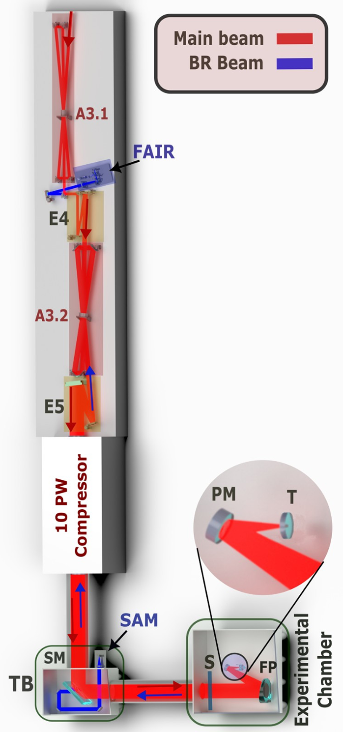
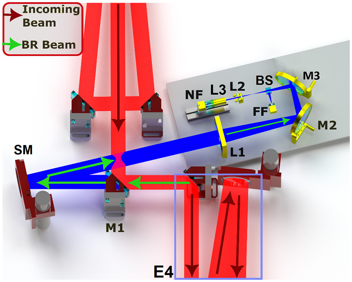
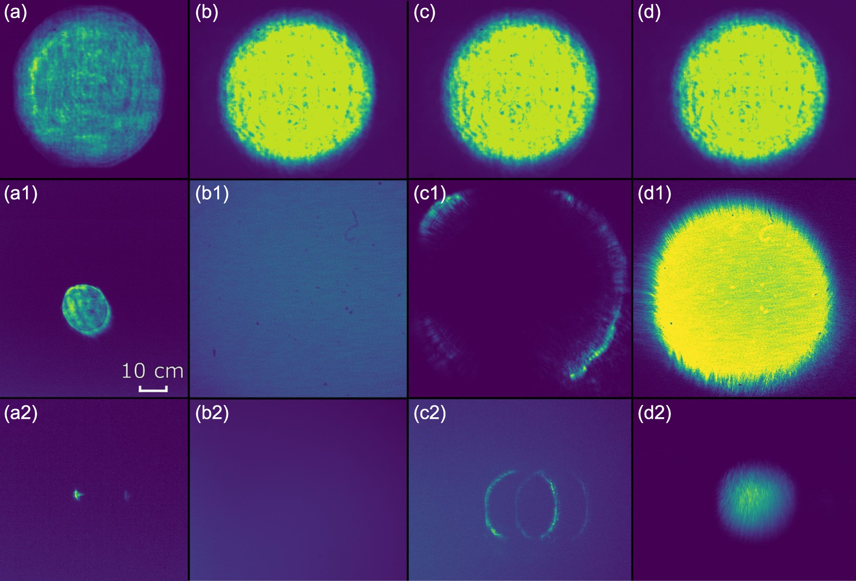
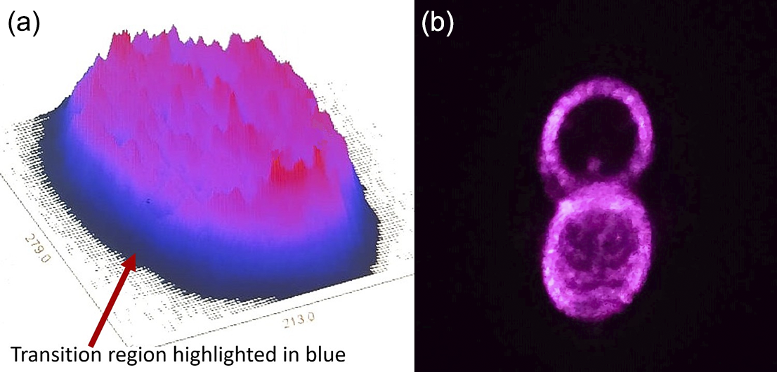
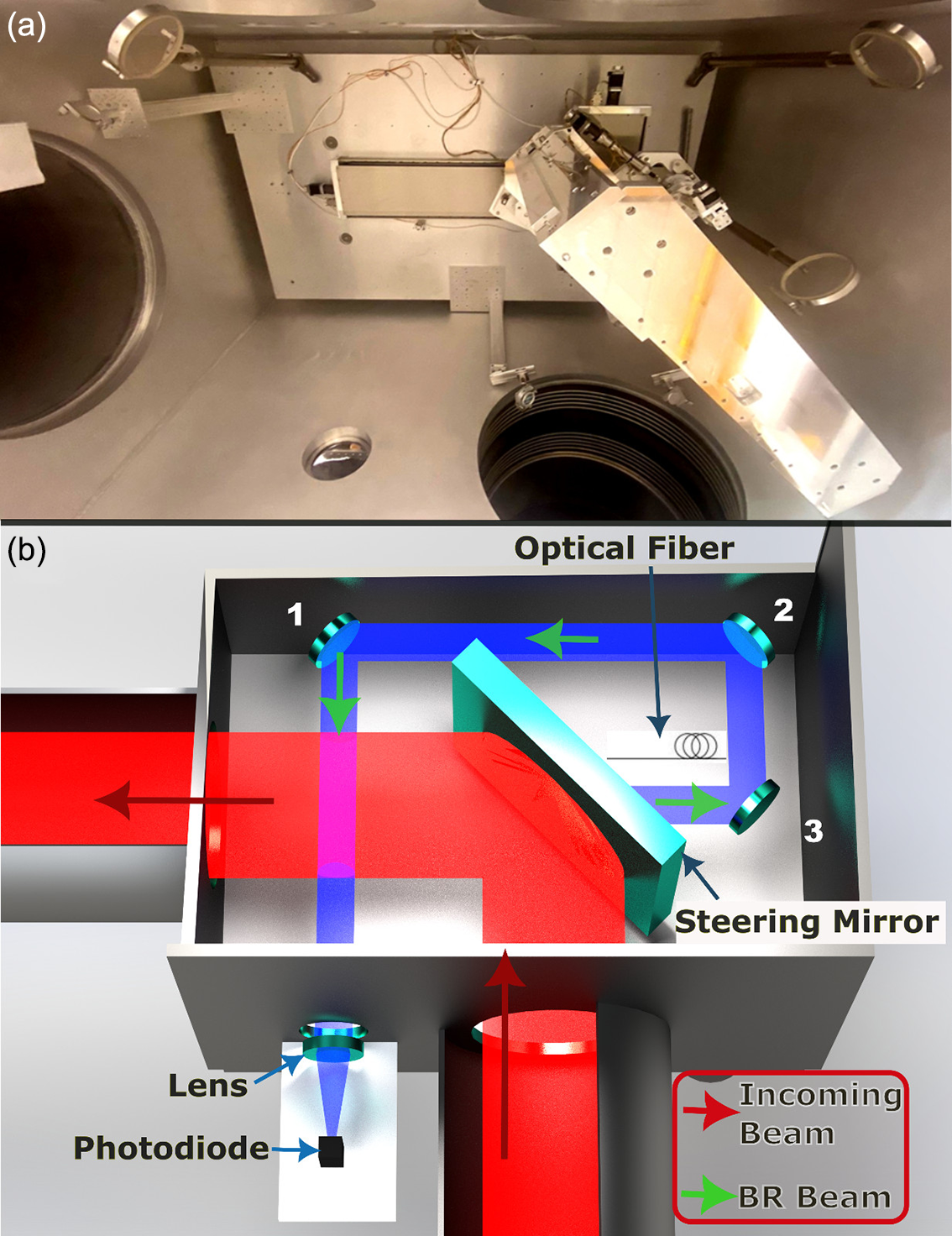
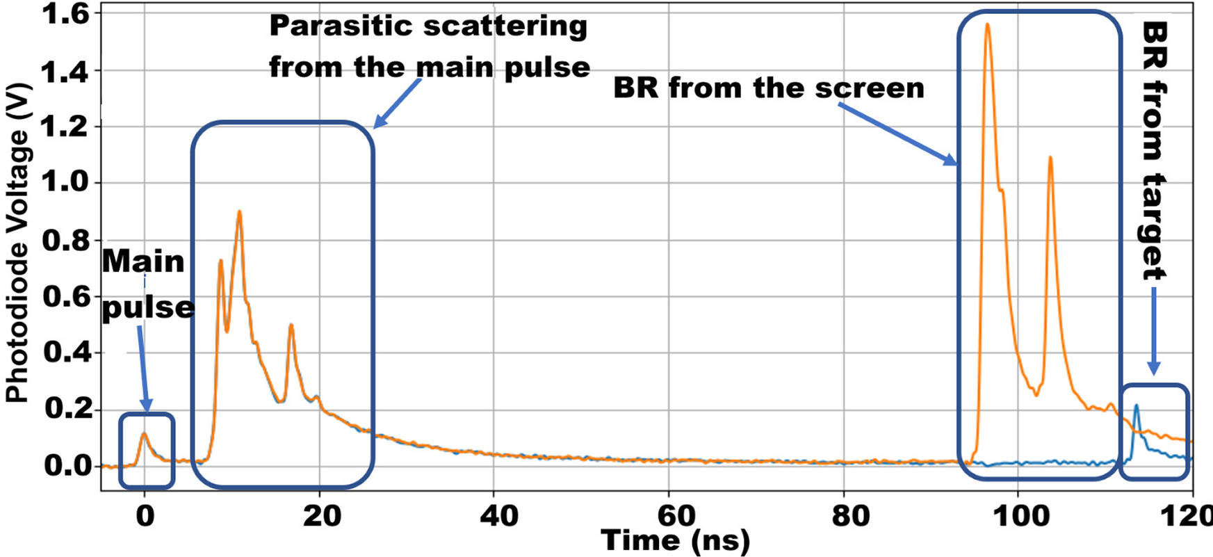
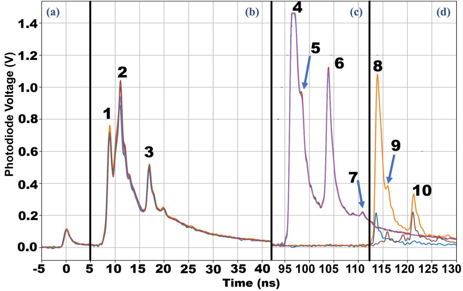
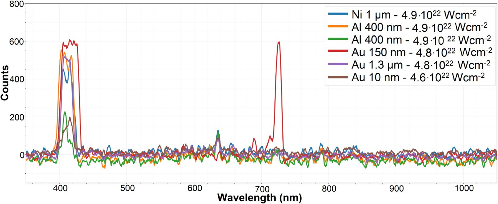


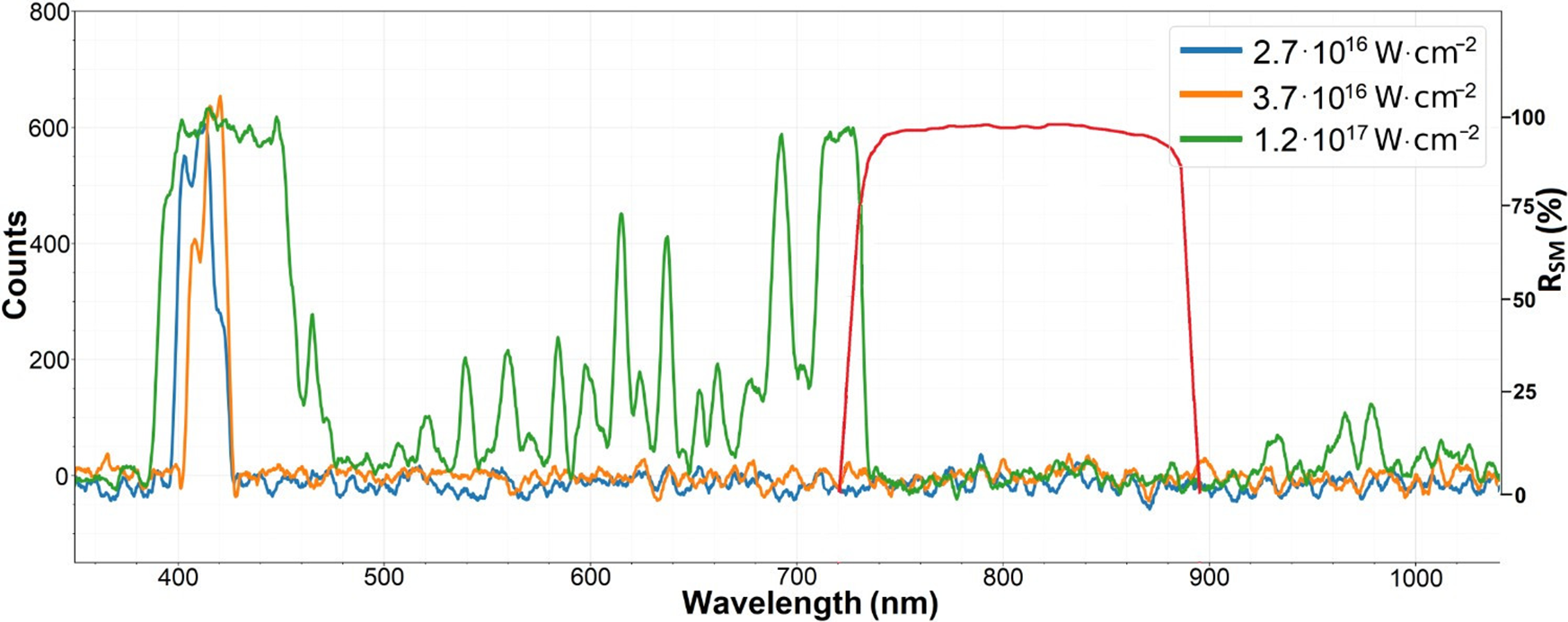


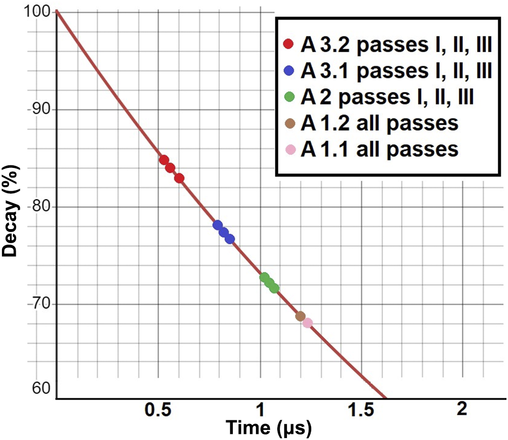
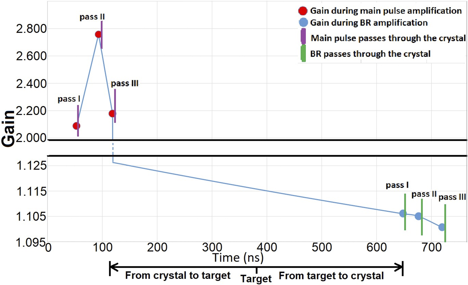
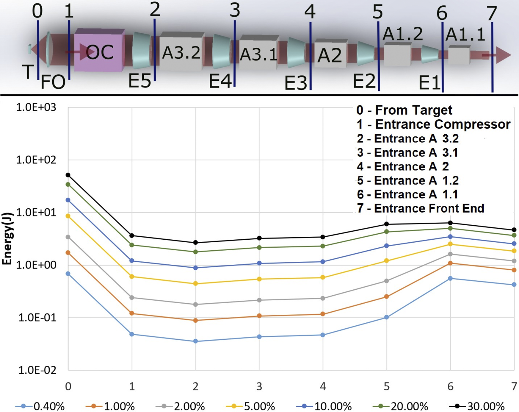
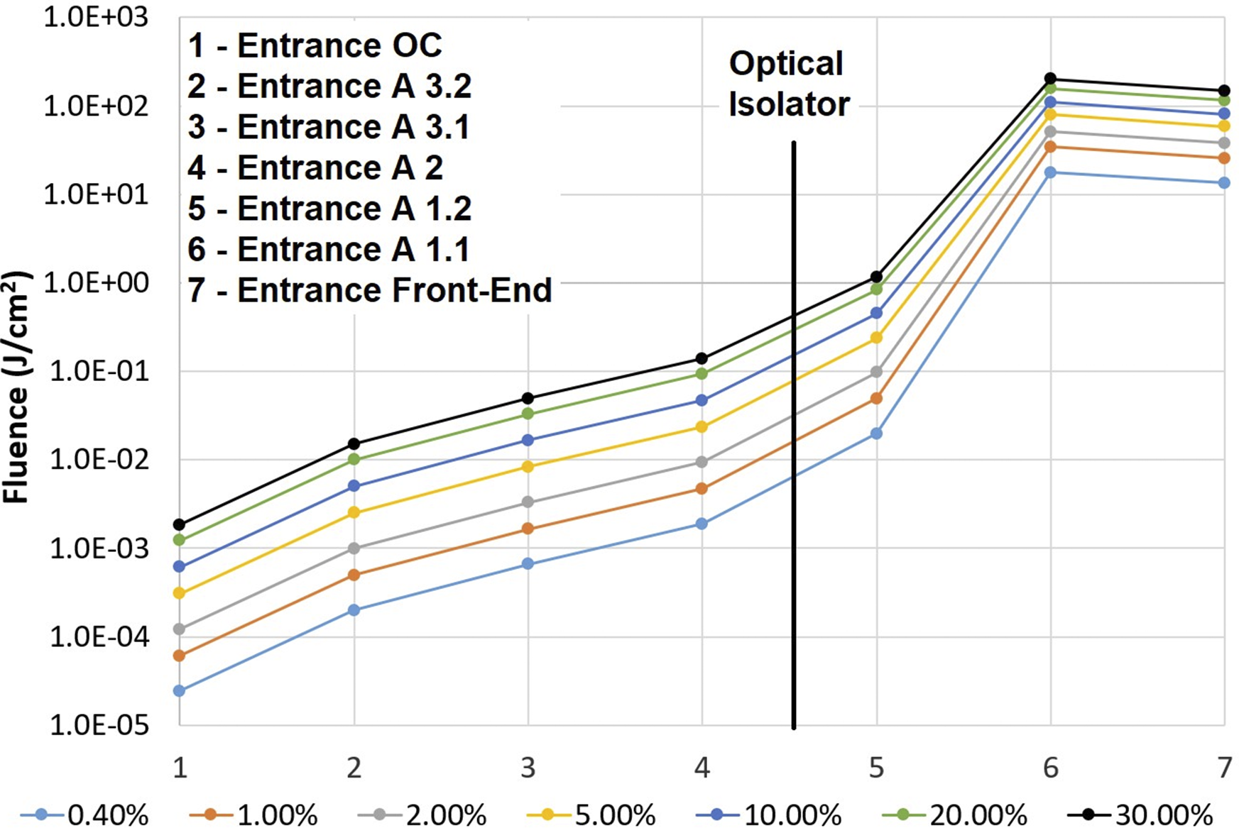

 Open access

