


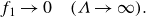
1. Introduction
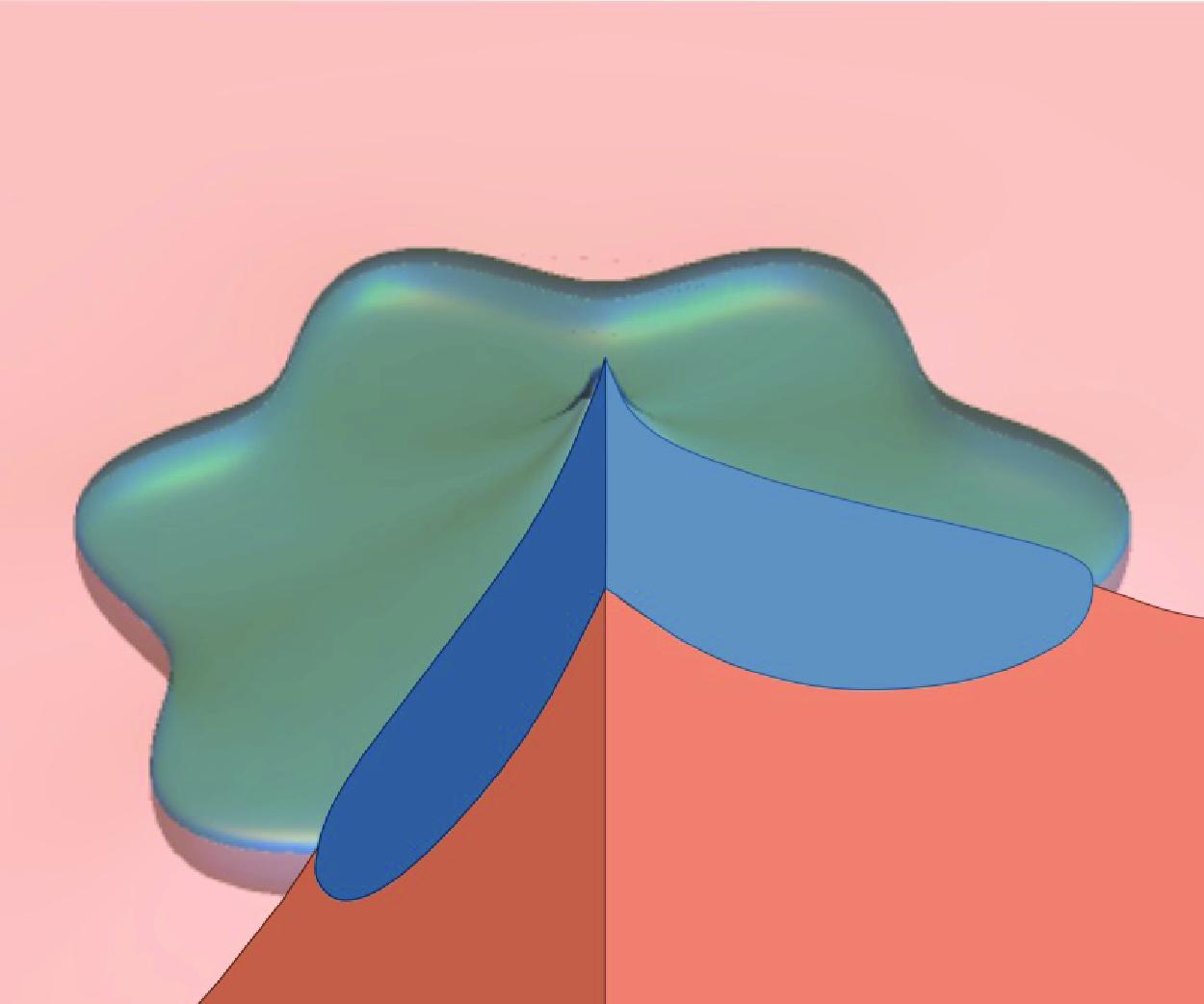
Viscous fingering instabilities involve complex, finger-like patterning that emerges when a less viscous fluid invades a more viscous fluid in a porous medium or Hele-Shaw cell (Saffman & Taylor Reference Saffman and Taylor1958; Homsy Reference Homsy1987). What has not been known until recently is that a similar type of viscous fingering instability also occurs in unconfined settings that do not involve porous media or Hele-Shaw cells. In particular, the interaction of the free-surface flows of two fluids of dissimilar viscosity manifests similar instabilities in various configurations depicted in figure 1( $b$
–
$b$
– $d$
). These configurations differ topologically from flows susceptible to classical viscous fingering instabilities, depicted in figure 1(
$d$
). These configurations differ topologically from flows susceptible to classical viscous fingering instabilities, depicted in figure 1( $a$
), through the lack of an upper rigid boundary, which brings with it the need to depart from the use of Darcy’s law for flow in porous media and the need to determine the upper free surface as part of the flow. Efforts to suppress this class of instabilities of free-surface flows while maintaining basal lubrication on the large scale led to the design of a structured substrate – a large-scale analogue of superhydrophobic substrates – which has been shown to give rise to a Navier-type slip macroscopically (Yan & Kowal Reference Yan and Kowal2024).
$a$
), through the lack of an upper rigid boundary, which brings with it the need to depart from the use of Darcy’s law for flow in porous media and the need to determine the upper free surface as part of the flow. Efforts to suppress this class of instabilities of free-surface flows while maintaining basal lubrication on the large scale led to the design of a structured substrate – a large-scale analogue of superhydrophobic substrates – which has been shown to give rise to a Navier-type slip macroscopically (Yan & Kowal Reference Yan and Kowal2024).
The first examined configuration (figure 1 $b$
) of flows susceptible to the novel instability involves the free-surface flow of a thin film of viscous fluid spreading beneath another viscous fluid, as seen in the experiments of Kowal & Worster (Reference Kowal and Worster2015, Reference Kowal and Worster2019a
,Reference Kowal and Worster
b
) and Kumar et al. (Reference Kumar, Zuri, Kogan, Gottlieb and Sayag2021). Such a flow becomes unstable to a novel cross-flow fingering instability when the intruding fluid is less viscous. Another configuration (figure 1
$b$
) of flows susceptible to the novel instability involves the free-surface flow of a thin film of viscous fluid spreading beneath another viscous fluid, as seen in the experiments of Kowal & Worster (Reference Kowal and Worster2015, Reference Kowal and Worster2019a
,Reference Kowal and Worster
b
) and Kumar et al. (Reference Kumar, Zuri, Kogan, Gottlieb and Sayag2021). Such a flow becomes unstable to a novel cross-flow fingering instability when the intruding fluid is less viscous. Another configuration (figure 1 $c$
), leading to similar instabilities, is one in which the intruding fluid fully displaces another viscous fluid (Kowal Reference Kowal2021). The final configuration (figure 1
$c$
), leading to similar instabilities, is one in which the intruding fluid fully displaces another viscous fluid (Kowal Reference Kowal2021). The final configuration (figure 1 $d$
) is one in which the intruding fluid spreads above a pre-existing thin film of viscous fluid, as seen in the experiments of Dauck (Reference Dauck2020), which focused on the limit in which the two layers are of equal density. We examine flows in the final configuration in the present paper, completing the family of flows susceptible to the novel frontal instability.
$d$
) is one in which the intruding fluid spreads above a pre-existing thin film of viscous fluid, as seen in the experiments of Dauck (Reference Dauck2020), which focused on the limit in which the two layers are of equal density. We examine flows in the final configuration in the present paper, completing the family of flows susceptible to the novel frontal instability.
Vertical cross-section of base flows susceptible to ( $a$
) classical viscous fingering instabilities (flows in a Hele-Shaw cell or other porous medium) and (
$a$
) classical viscous fingering instabilities (flows in a Hele-Shaw cell or other porous medium) and ( $b$
–
$b$
– $d$
) non-porous viscous fingering (free-surface flows). Fluid 1 is less viscous than fluid 2.
$d$
) non-porous viscous fingering (free-surface flows). Fluid 1 is less viscous than fluid 2.

Such free-surface flows are relevant to a range of phenomena involving the interaction of fluids of different viscosity. An example includes the nasal delivery of drugs and vaccines, which commonly results in what is referred to as nasal dripping in the medical community (Masiuk, Kadakia & Wang Reference Masiuk, Kadakia and Wang2016). Nasal dripping, or fingering, observed in this context results from the interaction of a low-viscosity drug solution or vaccine with a more viscous mucus. Such fingering is more pronounced the higher the viscosity ratio between the mucus and drug solution or vaccine, as observed in experiments involving synthetic mucus and the drug Avicel (Masiuk et al. Reference Masiuk, Kadakia and Wang2016). Other examples include the interaction between liquid sulphide and silicate melt in a partially solidified (or mostly unsolidified) magmatic system or, more generally, the interaction of lava flows of different viscosity following cooling (Fink & Griffiths Reference Fink and Griffiths1990, Reference Fink and Griffiths1998; Balmforth & Craster Reference Balmforth and Craster2000). Mention has also been made of a link to the flow of ice sheets over less viscous subglacial till, as explored theoretically and experimentally (Kumar et al. Reference Kumar, Zuri, Kogan, Gottlieb and Sayag2021; Gyllenberg & Sayag Reference Gyllenberg and Sayag2022).
The new class of instabilities of such free-surface flows have been termed non-porous viscous fingering instabilities, to reflect that they are not associated with porous media and that the mechanism of instability is similar to that of traditional viscous fingering instabilities, despite the lack of confinement (Kowal Reference Kowal2021). Such instabilities can be thought of as an ultrasoft analogue of fingering in soft/deformable porous media. The latter type of instability is partially suppressed by the elastic deformation of the porous medium or Hele-Shaw cell (Pihler-Puzovic et al. Reference Pihler-Puzovic, Illien, Heil and Juel2012, Reference Pihler-Puzovic, Perillat, Russell, Juel and Heil2013). A simple representation of such a deformable porous medium involves a horizontal Hele-Shaw cell in which its upper wall is replaced by an elastic sheet that is free to deform when a less viscous fluid is injected (Pihler-Puzovic et al. 2013, Reference Pihler-Puzovic, Perillat, Russell, Juel and Heil2013). Such instabilities are increasingly suppressed as the thickness of the sheet decreases. In this work, we remove the elastic sheet completely, falling into the realm of free-surface flows, rather than porous-media flows. Alternatively, we remove the upper wall of a rigid horizontal Hele-Shaw cell depicted in figure 1( $a$
). As a result, Darcy’s law no longer applies.
$a$
). As a result, Darcy’s law no longer applies.
Non-porous viscous fingering instabilities bring similarities to thermoviscous fingering of free-surface flows, in which the viscosity contrast required for onset of instability is driven thermally (Hindmarsh Reference Hindmarsh2004, Reference Hindmarsh2009; Algwauish & Naire Reference Algwauish and Naire2023). We also find it worthwhile to note the difference between non-porous viscous fingering instabilities and fingering of a driven spreading film (Huppert Reference Huppert1982a ; Troian et al. Reference Troian, Herbolzheimer, Safran and Joann1989). Although both of these involve frontal instabilities of free-surface flows, the former requires a viscosity difference between two fluids and the latter does not, as it involves a single fluid only. The latter instability is, importantly, one in which surface tension is key. As such, non-porous viscous fingering is more closely comparable to viscous fingering in porous media, despite no presence of a porous medium itself.
Viscous fingering in porous media, including Hele-Shaw cells, received considerable attention throughout the last few decades following the seminal work of Saffman & Taylor (Reference Saffman and Taylor1958). This stemmed mainly from its broad range of applications, ranging from enhanced oil recovery (Orr & Taber Reference Orr and Taber1984) to coating applications (Taylor Reference Taylor1963) and carbon sequestration (Cinar, Riaz & Tchelepi Reference Cinar, Riaz and Tchelepi2009). Similar instabilities are also frequently observed in nature, such as in crystal growth (Mullins & Sekerka Reference Mullins and Sekerka1964), the spreading of bacterial colonies (Ben-Jacob Reference Ben-Jacob1997), the dynamics of fractures (Hull Reference Hull1999) and the instability of flame fronts (Ben-Jacob et al. Reference Ben-Jacob, Schmueli, Shochet and Tenenbaum1992).
Interest has since emerged in the ability to either enhance or suppress these instabilities, and to manipulate the patterns that emerge, as desired, for industrial applications. Such control mechanisms have been found to depend upon a number of physical factors, including the injection rate of the less viscous fluid (Li et al. Reference Li, Lowengrub, Fontana and Palffy-Muhoray2009; Dias & Miranda Reference Dias and Miranda2010), the miscibility of the two fluids involved (Perkins, Johnston & Hoffman Reference Perkins, Johnston and Hoffman1965) and their rheology (Kondic, Shelley & Palffy-Muhoray Reference Kondic, Shelley and Palffy-Muhoray1998; Fast et al. Reference Fast, Kondic, Shelley and Palffy-Muhoray2001). Other effects that enhance or suppress these instabilities include changes in the viscosity ratio of the two fluids (Bischofberger, Ramachandran & Nagel Reference Bischofberger, Ramachandran and Nagel2014) and introducing particles (Luo, Chen & Lee Reference Luo, Chen and Lee2018), for instance. Alterations in the geometry of the porous medium also influence the fingering patterns, when the alterations are both static (Nase, Derks & Lindner Reference Nase, Derks and Lindner2011; Al-Housseiny, Tsai & Stone Reference Al-Housseiny, Tsai and Stone2012) and dynamic (Juel Reference Juel2012; Zheng, Kim & Stone Reference Zheng, Kim and Stone2015; Morrow, Moroney & McCue Reference Morrow, Moroney and McCue2019; Vaquero-Stainer et al. Reference Vaquero-Stainer, Heil, Juel and Pihler-Puzović2019).
There are a number of similarities between traditional viscous fingering instabilities in porous media and the recently discovered non-porous viscous fingering instabilities. Stability analyses (in the configuration of figure 1 $b$
) indicate that the latter instabilities emerge when the jump in hydrostatic pressure gradient across the intrusion front is negative (Kowal & Worster Reference Kowal and Worster2019a
,Reference Kowal and Worster
b
; Kowal Reference Kowal2021). This is similar to, yet contrasts with, traditional viscous fingering instabilities in porous media (figure 1
$b$
) indicate that the latter instabilities emerge when the jump in hydrostatic pressure gradient across the intrusion front is negative (Kowal & Worster Reference Kowal and Worster2019a
,Reference Kowal and Worster
b
; Kowal Reference Kowal2021). This is similar to, yet contrasts with, traditional viscous fingering instabilities in porous media (figure 1 $a$
), which are instead driven by a jump in dynamic pressure gradient (Homsy Reference Homsy1987). Both types of instabilities occur when the intruding viscous fluid is less viscous than the layer into which it intrudes, as has been seen in experiments in which the injected fluid intrudes from below (Kowal & Worster Reference Kowal and Worster2015, Reference Kowal and Worster2019a
,figure 1
$a$
), which are instead driven by a jump in dynamic pressure gradient (Homsy Reference Homsy1987). Both types of instabilities occur when the intruding viscous fluid is less viscous than the layer into which it intrudes, as has been seen in experiments in which the injected fluid intrudes from below (Kowal & Worster Reference Kowal and Worster2015, Reference Kowal and Worster2019a
,figure 1 $b$
) and from above (Dauck Reference Dauck2020, figure 1
$b$
) and from above (Dauck Reference Dauck2020, figure 1 $d$
). The latter experiments involved fluids of equal density. However, it has been found that non-zero density differences between the two layers of viscous fluid can suppress these instabilities when the injected fluid intrudes from below (Kowal & Worster Reference Kowal and Worster2019b
, figure 1
$d$
). The latter experiments involved fluids of equal density. However, it has been found that non-zero density differences between the two layers of viscous fluid can suppress these instabilities when the injected fluid intrudes from below (Kowal & Worster Reference Kowal and Worster2019b
, figure 1 $b$
). A similar observation has been found when the fluids are non-Newtonian (Leung & Kowal Reference Leung and Kowal2022b
, figure 1
$b$
). A similar observation has been found when the fluids are non-Newtonian (Leung & Kowal Reference Leung and Kowal2022b
, figure 1 $b$
).
$b$
).
In this work, we demonstrate similar suppression when the intruding fluid is supplied from above, as depicted in figure 1( $d$
). In particular, we examine the formation of viscous fingering instabilities that emerge when a viscous gravity current intrudes radially outwards over another thin film of viscous fluid, where the two fluids are of unequal densities and viscosities. By conducting a linear stability analysis using the axisymmetric similarity solutions of the companion paper Yang, Mottram & Kowal (Reference Yang, Mottram and Kowal2024) as the base flow, we characterise the parameter space over which these instabilities occur. We also compare these instabilities with related fingering instabilities that emerge when the injected fluid intrudes from below. To formulate the problem, we build directly upon the framework of Dauck et al. (Reference Dauck, Box, Gell, Neufeld and Lister2019) and Yang et al. (Reference Yang, Mottram and Kowal2024) by allowing for variations in the azimuthal direction. We also refer to the experiments of Dauck (Reference Dauck2020), where similar frontal instabilities emerge. The linear stability analysis of Dauck (Reference Dauck2020), focusing on the limit in which the two layers are of equal density, also confirms these instabilities but did not reveal a most unstable wavenumber, much like the equal-density stability calculations of Kowal & Worster (Reference Kowal and Worster2019b
) when the less viscous fluid intrudes from below and growth rates increase with the wavenumber indefinitely. Interestingly, no instabilities were observed in related experiments of Lister & Kerr (Reference Lister and Kerr1989), involving a thin film of viscous fluid intruding at a fluid interface, save for small-scale frontal patterning attributed to contamination of the fluid surface by dust. We find through our stability calculations that the parameter regime in which the latter experiments were performed corresponds to stable configurations. Other relevant works include single-layer (Smith Reference Smith1969; Huppert Reference Huppert1982a
,Reference Huppert
b
) and two-layer (Kowal & Worster Reference Kowal and Worster2015; Dauck et al. Reference Dauck, Box, Gell, Neufeld and Lister2019; Shah, Pegler & Minchew Reference Shah, Pegler and Minchew2021) flows over horizontal and inclined substrates, and non-Newtonian analogues (Hewitt Reference Hewitt2013; Gyllenberg & Sayag Reference Gyllenberg and Sayag2022; Hinton Reference Hinton2022; Christy & Hinton Reference Christy and Hinton2023), to name a few.
$d$
). In particular, we examine the formation of viscous fingering instabilities that emerge when a viscous gravity current intrudes radially outwards over another thin film of viscous fluid, where the two fluids are of unequal densities and viscosities. By conducting a linear stability analysis using the axisymmetric similarity solutions of the companion paper Yang, Mottram & Kowal (Reference Yang, Mottram and Kowal2024) as the base flow, we characterise the parameter space over which these instabilities occur. We also compare these instabilities with related fingering instabilities that emerge when the injected fluid intrudes from below. To formulate the problem, we build directly upon the framework of Dauck et al. (Reference Dauck, Box, Gell, Neufeld and Lister2019) and Yang et al. (Reference Yang, Mottram and Kowal2024) by allowing for variations in the azimuthal direction. We also refer to the experiments of Dauck (Reference Dauck2020), where similar frontal instabilities emerge. The linear stability analysis of Dauck (Reference Dauck2020), focusing on the limit in which the two layers are of equal density, also confirms these instabilities but did not reveal a most unstable wavenumber, much like the equal-density stability calculations of Kowal & Worster (Reference Kowal and Worster2019b
) when the less viscous fluid intrudes from below and growth rates increase with the wavenumber indefinitely. Interestingly, no instabilities were observed in related experiments of Lister & Kerr (Reference Lister and Kerr1989), involving a thin film of viscous fluid intruding at a fluid interface, save for small-scale frontal patterning attributed to contamination of the fluid surface by dust. We find through our stability calculations that the parameter regime in which the latter experiments were performed corresponds to stable configurations. Other relevant works include single-layer (Smith Reference Smith1969; Huppert Reference Huppert1982a
,Reference Huppert
b
) and two-layer (Kowal & Worster Reference Kowal and Worster2015; Dauck et al. Reference Dauck, Box, Gell, Neufeld and Lister2019; Shah, Pegler & Minchew Reference Shah, Pegler and Minchew2021) flows over horizontal and inclined substrates, and non-Newtonian analogues (Hewitt Reference Hewitt2013; Gyllenberg & Sayag Reference Gyllenberg and Sayag2022; Hinton Reference Hinton2022; Christy & Hinton Reference Christy and Hinton2023), to name a few.
We begin with a theoretical development in § 2, in which the geometry of the problem, the assumptions and the governing equations are laid out. We investigate the stability of the flow to small non-axisymmetric disturbances by performing a linear stability analysis in § 3, in which we also derive asymptotic solutions for perturbations around a stress singularity at the injection front. We solve the resulting perturbation equations numerically, characterise the instability across parameter space and further discuss our results in § 4. We finalise with concluding remarks in § 5.
2. Theoretical development
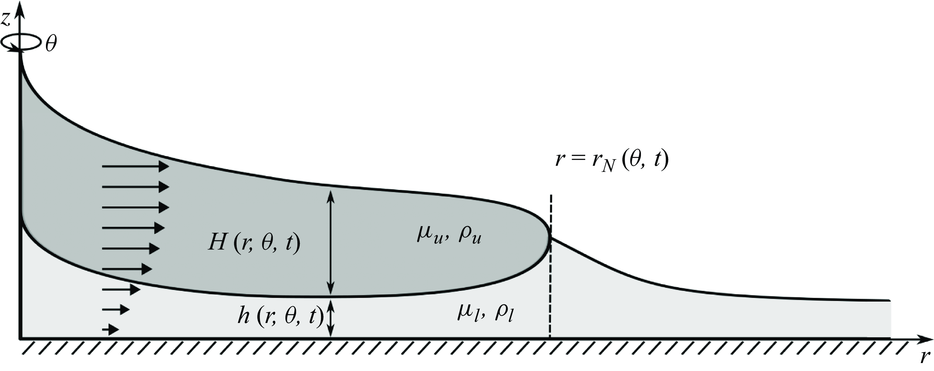
As depicted in figure 2, we consider the flow of two thin films of incompressible, Newtonian viscous fluids of constant viscosities $\mu _u$
and
$\mu _u$
and $\mu _l$
and constant densities
$\mu _l$
and constant densities $\rho _u$
and
$\rho _u$
and $\rho _l$
in an axisymmetric geometry. The subscripts
$\rho _l$
in an axisymmetric geometry. The subscripts $_u$
and
$_u$
and $_l$
correspond to quantities involving the upper and lower layers, respectively. The subscript
$_l$
correspond to quantities involving the upper and lower layers, respectively. The subscript $_l$
also describes quantities ahead of the intrusion front. We assume that the effects of inertia and surface tension are negligible and that both fluid layers are long and thin, and are resisted dominantly by vertical shear stresses within the limits of lubrication theory.
$_l$
also describes quantities ahead of the intrusion front. We assume that the effects of inertia and surface tension are negligible and that both fluid layers are long and thin, and are resisted dominantly by vertical shear stresses within the limits of lubrication theory.
Schematic of a thin film of viscous fluid spreading over a lubricated substrate in an axisymmetric geometry. Schematic adapted from Yang et al. (Reference Yang, Mottram and Kowal2024).
We note that the use of the lubrication approximation reflects an idealised scenario in which only vertical shear stress appears, and we aim to determine whether or not this suffices to explain the emergence of instability. Strictly speaking, the approximations of lubrication theory break down at the nose, where there is a frontal stress singularity, thus warranting the need for the solution of the full Stokes equations near the nose. We do not attempt this in this paper. We note that the experiments of Dauck (Reference Dauck2020), performed in a similar configuration to the present paper, and their close agreement to theoretical predictions (which make use of lubrication theory) for their propagation and shape (Dauck et al. Reference Dauck, Box, Gell, Neufeld and Lister2019; Dauck Reference Dauck2020), give credence to the use of lubrication theory at least as a first attempt upon which higher-order corrections can be made in the future. Another similar example is the experiments and stability analysis of Kowal & Worster (Reference Kowal and Worster2019b ), which similarly made use of the lubrication approximation, albeit in a different configuration (in that the less viscous fluid intrudes from below rather than from above).
The two fluids are supplied at constant fluxes $\hat {\mathcal{Q}}_u$
and
$\hat {\mathcal{Q}}_u$
and $\hat {\mathcal{Q}}_l$
at the origin and spread radially outwards over a horizontal, rigid substrate, which is prewetted by the lower-layer fluid to an initial, uniform depth
$\hat {\mathcal{Q}}_l$
at the origin and spread radially outwards over a horizontal, rigid substrate, which is prewetted by the lower-layer fluid to an initial, uniform depth $h_\infty$
. While the two fluids spread radially outwards, we allow for non-axisymmetric variations in the flow. The upper current extends to the intrusion front
$h_\infty$
. While the two fluids spread radially outwards, we allow for non-axisymmetric variations in the flow. The upper current extends to the intrusion front $r = r_N(\theta , t)$
, which splits the domain into two regions: a two-layer region
$r = r_N(\theta , t)$
, which splits the domain into two regions: a two-layer region $0\lt r\lt r_N$
, involving both viscous fluids, and a single-layer region
$0\lt r\lt r_N$
, involving both viscous fluids, and a single-layer region $r\gt r_N$
, involving a single viscous fluid of the same material properties as the underlying layer of the two-layer region. The thicknesses of the upper and lower layers are denoted by
$r\gt r_N$
, involving a single viscous fluid of the same material properties as the underlying layer of the two-layer region. The thicknesses of the upper and lower layers are denoted by $H(r,\theta ,t)$
and
$H(r,\theta ,t)$
and $h(r,\theta ,t)$
, respectively.
$h(r,\theta ,t)$
, respectively.
Applying the standard lubrication approximation (see Yang et al. (Reference Yang, Mottram and Kowal2024)for details of the derivation in the axisymmetric case) results in the following mass conservation equations:
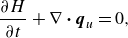 \begin{align}& \frac {\partial H}{\partial t} + \nabla \boldsymbol{\cdot }\boldsymbol{q}_u = 0, \end{align}
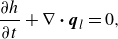 \begin{align}&\, \frac {\partial h}{\partial t} + \nabla \boldsymbol{\cdot } \boldsymbol{q}_l = 0, \end{align}
within the two layers, where the depth-integrated fluxes of upper- and lower-layer fluid are given by
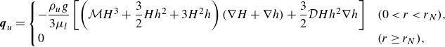 \begin{align}& \boldsymbol{q}_u = \begin{cases} -\dfrac {\rho _ug}{3\mu _l}\left [\left (\mathcal{M}H^3+\dfrac {3}{2}H h^2+3H^2 h\right )(\nabla H+\nabla h)+\dfrac {3}{2}\mathcal{D} H h^2\nabla h\right ] & (0\lt r\lt r_N),\\ 0 & (r\geq r_N), \end{cases} \end{align}
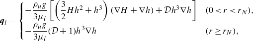 \begin{align}&\qquad\quad \boldsymbol{q}_l =\begin{cases} -\dfrac {\rho _ug}{3\mu _l}\left [\left (\dfrac {3}{2}H h^2+h^3\right )( \nabla H+\nabla h )+\mathcal{D}h^3\nabla h\right ] & (0\lt r\lt r_N),\\[8pt] -\dfrac {\rho _ug}{3\mu _l}(\mathcal{D}+1)h^3\nabla h & (r\geq r_N), \end{cases} \end{align}
in terms of the dimensionless parameters
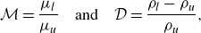 \begin{equation} \mathcal{M} = \frac {\mu _l}{\mu _u}\quad \text{and} \quad \mathcal{D} = \frac {\rho _l-\rho _u}{\rho _u}, \end{equation}
which denote the viscosity ratio and relative density difference, respectively. In general, the quantities described here may vary in $\theta$
. Here, g refers to the gravitational acceleration.
$\theta$
. Here, g refers to the gravitational acceleration.
At the origin, $r=0$
, we assume that the upper and lower layers are supplied at a constant flux
$r=0$
, we assume that the upper and lower layers are supplied at a constant flux $\hat {\mathcal{Q}}_l$
,
$\hat {\mathcal{Q}}_l$
, $\hat {\mathcal{Q}}_u$
, respectively, so that
$\hat {\mathcal{Q}}_u$
, respectively, so that
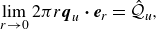 \begin{align} \lim _{r\rightarrow 0} 2 \pi r \boldsymbol{q}_u \boldsymbol{\cdot } \boldsymbol{e}_r &= \hat {\mathcal{Q}}_u, \end{align}
 \begin{align} \lim _{r\rightarrow 0} 2 \pi r \boldsymbol{q}_l \boldsymbol{\cdot }\boldsymbol{e}_r &= \hat {\mathcal{Q}}_l, \end{align}
where $\boldsymbol{e}_r$
is the radial unit basis vector.
$\boldsymbol{e}_r$
is the radial unit basis vector.
The thickness and the normal flux of the lower layer are continuous across the intrusion front $r = r_N(\theta ,t)$
, so that
$r = r_N(\theta ,t)$
, so that
 \begin{align}&\quad [h]^+_- = 0\ \ \ \ \mathrm{at}\ r=r_N, \end{align}
 \begin{align}& [\boldsymbol{q}_l\boldsymbol{\cdot } \boldsymbol{n}]^+_-= 0\ \ \ \ \mathrm{at}\ r=r_N, \end{align}
where $\boldsymbol{n}$
is the outward unit normal vector to the intrusion front. In addition, the normal component of the upper-layer flux vanishes at the front, so that
$\boldsymbol{n}$
is the outward unit normal vector to the intrusion front. In addition, the normal component of the upper-layer flux vanishes at the front, so that
 \begin{equation} \boldsymbol{q}_u\boldsymbol{\cdot } \boldsymbol{n} = 0\ \ \ \ \mathrm{at}\ r=r_N. \end{equation}
The front evolves kinematically, so that
 \begin{equation} \dot {r}_N = \lim _{r\to r_N^-} H^{-1}\boldsymbol{q}_u \boldsymbol{\cdot } \boldsymbol{\nabla }(r-r_N) = \lim _{r\rightarrow r_N^-} \left [\frac {\boldsymbol{q}_u\boldsymbol{\cdot } \boldsymbol{e}_r}{H}-\frac {\boldsymbol{q}_u\boldsymbol{\cdot } \boldsymbol{e_\theta } }{Hr_N}\frac {\partial r_N}{\partial \theta }\right ]. \end{equation}
Here, $\boldsymbol{e}_\theta$
is the azimuthal unit basis vector. In the far field, we assume that the thickness is uniform so that
$\boldsymbol{e}_\theta$
is the azimuthal unit basis vector. In the far field, we assume that the thickness is uniform so that
 \begin{equation} \lim _{r\rightarrow \infty }h = h_\infty . \end{equation}
These governing equations, boundary conditions, matching conditions, and the evolution equation for the front fully specify the moving boundary problem considered in this paper.
3. Non-axisymmetric disturbances
We investigate the evolution of non-axisymmetric disturbances of the base flow by expanding about the zeroth-order axisymmetric similarity solutions of Yang et al. (Reference Yang, Mottram and Kowal2024). To do so, we change the independent variables $(r,\theta ,t)$
to
$(r,\theta ,t)$
to $(\xi , \vartheta , \tau )$
and non-dimensionalise the system by applying the following transformations
$(\xi , \vartheta , \tau )$
and non-dimensionalise the system by applying the following transformations
 \begin{align} &(\xi , \xi _N(\vartheta ,\tau )) = \left (\frac {3\mu _l}{\rho _u g h_{\infty }^3 t}\right )^{1/2} (r,r_N(\theta ,t)) ,\quad \vartheta =\theta ,\quad \tau = \log (t/t_0), \end{align}
 \begin{align} &\qquad\quad\,\,\, \left (F(\xi , \vartheta , \tau ),f(\xi , \vartheta , \tau )\right ) = h_{\infty }^{-1}\left (H(r,\theta ,t),h(r,\theta ,t)\right ), \end{align}
 \begin{align} &\,\,\, \left (\boldsymbol{\phi }_u(\xi , \vartheta , \tau ),\boldsymbol{\phi }_l(\xi , \vartheta , \tau )\right ) = \left (\frac {3\mu _l\, t}{\rho _u g h_{\infty }^5 }\right )^{1/2}\left (\boldsymbol{q}_u(r,\theta ,t),\boldsymbol{q}_l(r,\theta ,t)\right ), \end{align}
where $t_0=3 \mu _l / (\rho _u g h_{\infty } )$
. We also rescale the two input source fluxes at the origin so that
$t_0=3 \mu _l / (\rho _u g h_{\infty } )$
. We also rescale the two input source fluxes at the origin so that
 \begin{equation} \mathcal{Q}_u = \hat {\mathcal{Q}}_u /\hat {\mathcal{Q}} \quad \text{and} \quad \mathcal{Q}_l = \hat {\mathcal{Q}}_l /\hat {\mathcal{Q}}, \end{equation}
where
 \begin{equation} \hat {\mathcal{Q}} =2\pi h_{\infty }^4 \frac {\rho _u g}{3\mu _l} \end{equation}
is a dimensional measure of the lower-layer flux associated with a depth of $h_{\infty }$
. Alternatively, the parameter
$h_{\infty }$
. Alternatively, the parameter $\hat {\mathcal{Q}}$
can be interpreted as the flux required to attain a thickness of
$\hat {\mathcal{Q}}$
can be interpreted as the flux required to attain a thickness of $h_\infty$
near the source.
$h_\infty$
near the source.
The transformation (3.1)–(3.3) into similarity space transforms the base flow (the similarity solutions of Yang et al. (Reference Yang, Mottram and Kowal2024)) into a steady solution, which is key to allow a straightforward stability analysis to be performed. This can be seen by examining the transformed system of partial differential equations
 \begin{align} & \frac {\partial F}{\partial \tau }-\frac {1}{2}{\frac {\partial F}{\partial \xi }}\xi + \frac {1}{\xi } {\frac {\partial (\xi \phi _{ur})}{\partial \xi }}+\frac {1}{\xi }\frac {\partial \phi _{u\theta }}{\partial \vartheta } = 0, \end{align}
 \begin{align} &\,\, \frac {\partial f}{\partial \tau }-\frac {1}{2}{\frac {\partial f}{\partial \xi }}\xi + \frac {1}{\xi } {\frac {\partial (\xi \phi _{lr})}{\partial \xi }}+\frac {1}{\xi }\frac {\partial \phi _{l\theta }}{\partial \vartheta } = 0, \end{align}
describing mass conservation within the two layers of viscous fluid, the coefficients of which are independent of the transformed time variable $\tau$
. Here, the radial and azimuthal components of the depth-integrated fluxes of the two layers of fluid are given by
$\tau$
. Here, the radial and azimuthal components of the depth-integrated fluxes of the two layers of fluid are given by
 \begin{align} &\, (\phi _{ur},\phi _{lr}) = (\boldsymbol{\phi }_u \boldsymbol{\cdot } \boldsymbol{e}_r,\;\; \boldsymbol{\phi }_l\boldsymbol{\cdot } \boldsymbol{e}_r), \end{align}
 \begin{align} & ({\phi _{u\theta }},\phi _{l\theta }) = (\boldsymbol{\phi }_u\boldsymbol{\cdot } \boldsymbol{e}_\theta , \;\; \boldsymbol{\phi }_l\boldsymbol{\cdot } \boldsymbol{e}_\theta ), \end{align}
where
 \begin{align} & \boldsymbol{\phi }_u=\begin{cases} -\left [ \left (\mathcal{M}F^3+\dfrac {3}{2}F f^2+3F^2 f\right )(\nabla F+\nabla f)+\dfrac {3}{2}\mathcal{D} F f^2\nabla f\right ] & (0\lt \xi \lt \xi _N)\\ 0 & (\xi \geq \xi _N), \end{cases} \end{align}
 \begin{align} &\qquad\quad \boldsymbol{\phi }_{l} = \begin{cases} -\left [\left (\dfrac {3}{2}F f^2+f^3\right )( \nabla F+\nabla f )+\mathcal{D}f^3\nabla f\right ] & (0\lt \xi \lt \xi _N)\\ \\[-8pt] -(\mathcal{D}+1)f^3\nabla f & (\xi \geq \xi _N), \end{cases} \end{align}
for the upper and lower layers, respectively. The operator $\nabla$
is now the gradient operator in the two-dimensional polar coordinate system spanned by
$\nabla$
is now the gradient operator in the two-dimensional polar coordinate system spanned by $(\xi ,\vartheta )$
.
$(\xi ,\vartheta )$
.
As for the boundary conditions, the source flux boundary conditions reduce to
 \begin{gather} \xi \phi _{ur} \rightarrow \mathcal{Q}_u,\ \ \ \ \xi \phi _{lr} \rightarrow \mathcal{Q}_l\quad (\xi \rightarrow 0), \end{gather}
while the matching conditions at the intrusion front, describing continuity of lower-layer thickness, continuity of lower-layer flux and the zero-flux condition for the upper layer, are given by
 \begin{gather} [f]^+_- = 0,\ \ \ \ [\boldsymbol{\phi }_l\cdot \boldsymbol{n}]^+_-= 0,\ \ \ \ \boldsymbol{\phi }_u\cdot \boldsymbol{n}= 0\ \ \ \ (\xi = \xi _N), \end{gather}
respectively, where the normal vector at the intrusion front becomes
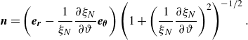 \begin{equation} \boldsymbol{n}=\left (\boldsymbol{e_r}-\frac {1}{\xi _N}{\frac {\partial \xi _N}{\partial \vartheta }}\boldsymbol{e_\theta }\right ) \left ( 1+\left (\frac {1}{\xi _N}{\frac {\partial \xi _N}{\partial \vartheta }}\right )^2 \right )^{-1/2}. \end{equation}
These are supplemented by the kinematic condition, which reduces to
 \begin{gather} \frac { \boldsymbol{e_r}\boldsymbol{\cdot }\boldsymbol{\phi }_u}{F}-\frac {1}{\xi _N}{\frac {\partial \xi _N}{\partial \vartheta }}\frac {\boldsymbol{e_\theta }\boldsymbol{\cdot }\boldsymbol{\phi }_u}{F} \rightarrow \frac {\partial \xi _N}{\partial \tau }+\frac {1}{2}\xi _N \ \ \ \ (\xi \rightarrow \xi _N^-), \end{gather}
and the far-field condition,
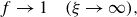 \begin{gather} f \rightarrow 1\ \ \ \ (\xi \rightarrow \infty ), \end{gather}
reflecting the choice to scale vertical lengths with respect to the dimensional far-field thickness.
These governing equations are a set of nonlinear partial differential equations describing the flow of general disturbances to the axisymmetric base flow. In a later section, we will focus on small-amplitude disturbances and linearise these equations about the base flow. However, the singular structure of the intrusion front raises problems with formulating the small-amplitude equations and boundary conditions consistently. To avoid these issues, we first investigate the structure of the singularity at the intrusion front in the following section, and then use it to make an informed coordinate transformation that will allow for a consistent set of small-amplitude equations and boundary conditions to be formulated.
3.1. Frontal singularity and asymptotic solution
Similar to the behaviour of the unperturbed, axisymmetric flow (the basic state considered in Yang et al. (Reference Yang, Mottram and Kowal2024)), there is a frontal singularity inherent to the perturbed flow. We generalise the asymptotic analysis of Yang et al. (Reference Yang, Mottram and Kowal2024)for the unperturbed flow near the intrusion front to include variations in the azimuthal direction and find a generalised asymptotic solution near the front of the form
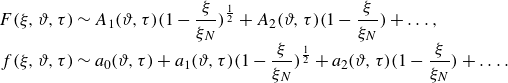 \begin{equation} \begin{aligned} F(\xi ,\vartheta ,\tau ) &\sim A_1(\vartheta ,\tau )\bigg(1-\frac {\xi }{\xi _N}\bigg)^{\frac {1}{2}}+A_2(\vartheta ,\tau )\bigg(1-\frac {\xi }{\xi _N}\bigg)+\ldots , \\[-3pt] f(\xi ,\vartheta ,\tau ) &\sim a_0(\vartheta ,\tau )+a_1(\vartheta ,\tau )\bigg(1-\frac {\xi }{\xi _N}\bigg)^{\frac {1}{2}}+a_2(\vartheta ,\tau )\bigg(1-\frac {\xi }{\xi _N}\bigg)+\ldots . \end{aligned} \end{equation}
reflecting a square-root singularity, in contrast to the cube-root frontal singularity of a single-layer viscous gravity current (Huppert Reference Huppert1982b
). Here, the relationships between the coefficients $a_0, a_1, a_2, A_1$
and
$a_0, a_1, a_2, A_1$
and $A_2$
are given by
$A_2$
are given by
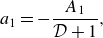 \begin{align}&\qquad\qquad\qquad\qquad\qquad\qquad a_1 = -\frac {A_1}{\mathcal{D}+1}, \end{align}
 \begin{align}&\qquad\qquad\qquad\qquad\quad A_2 = -\frac {4A_1^2}{9 a_0}\bigg(\mathcal{M}-\frac {3}{\mathcal{D}+1}\bigg), \end{align}
 \begin{align}& a_2 = \frac {1}{9 (\mathcal{D}+1) a_0^2 }\bigg[3 \xi _N \bigg(\xi _N+2 \frac {\partial \xi _N}{\partial \tau } \bigg) + A_1^2 a_0 \bigg( 4 \mathcal{M}-9-\frac {3}{\mathcal{D}+1}\bigg) \bigg]. \end{align}
As the base flow involves a singularity at the intrusion front, singular terms appear also in the equations governing the perturbations. This prevents one from formulating consistent linearised boundary conditions at the front. A similar problem occurs when linearising about the Barenblatt–Pattle similarity solution and various methods have been introduced to handle it, including the use of the method of strained coordinates (Grundy & McLaughlin Reference Grundy and McLaughlin1982) and a transformation of the dependent variable (Mathunjwa & Hogg Reference Mathunjwa and Hogg2006). Instead, we follow an approach similar to that of Kowal & Worster (Reference Kowal and Worster2019b
) by simply mapping the two-layer region to a fixed interval $[0,1]$
via the coordinate transformation
$[0,1]$
via the coordinate transformation
 \begin{equation} \Lambda = \xi /\xi _N. \end{equation}
Such a coordinate transformation eliminates the need to perturb the position of the singular point, which is now fixed at $\Lambda =1$
, for the corresponding boundary conditions. We summarise the equations and boundary conditions for the small-amplitude perturbations in terms of
$\Lambda =1$
, for the corresponding boundary conditions. We summarise the equations and boundary conditions for the small-amplitude perturbations in terms of $\Lambda$
in the following section. However, to aid numerical integration, we further transform the independent variable nonlinearly by defining
$\Lambda$
in the following section. However, to aid numerical integration, we further transform the independent variable nonlinearly by defining
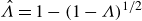 \begin{equation} \hat \Lambda = 1-(1-\Lambda )^{1/2} \end{equation}
in the two-layer region and $\hat \Lambda = \Lambda$
in the single-layer region. The transformation (3.22) is motivated by our asymptotic solution (3.17), which identifies a square-root singularity near the front. Under the transformation (3.22), the thicknesses of the two layers are instead linear near the intrusion front, and hence their gradients no longer diverge. In essence, the frontal singularity is now a removable singularity, which is simpler to handle numerically.
$\hat \Lambda = \Lambda$
in the single-layer region. The transformation (3.22) is motivated by our asymptotic solution (3.17), which identifies a square-root singularity near the front. Under the transformation (3.22), the thicknesses of the two layers are instead linear near the intrusion front, and hence their gradients no longer diverge. In essence, the frontal singularity is now a removable singularity, which is simpler to handle numerically.
3.2. Small-amplitude perturbations
We wish to examine the evolution of small pertubations to the base, axisymmetric flow, and in order to do so, we linearise the transformed problem by defining
 \begin{equation} X(\xi ,\vartheta ,\tau )\equiv X(\Lambda ,\Theta ,\mathcal{T}\kern1pt) =X_0(\Lambda ) +\epsilon \tilde {X}_1(\Lambda ,\Theta ,\mathcal{T}\kern1pt)+\ldots \end{equation}
for variables $X = f,F,\phi _{ur}, \phi _{u\theta }, \phi _{lr}, \phi _{l\theta }, \boldsymbol{\phi }_l,\boldsymbol{\phi }_u$
, where
$X = f,F,\phi _{ur}, \phi _{u\theta }, \phi _{lr}, \phi _{l\theta }, \boldsymbol{\phi }_l,\boldsymbol{\phi }_u$
, where $\epsilon$
is an arbitrary small number,
$\epsilon$
is an arbitrary small number, $\Theta = \vartheta$
,
$\Theta = \vartheta$
, $\mathcal{T} = \tau$
and
$\mathcal{T} = \tau$
and
 \begin{equation} \chi = \chi _0+\epsilon \tilde {\chi }_1(\Theta ,\mathcal{T}\kern1pt)+\ldots \end{equation}
for variables $\chi = \xi _N, a_0, a_1, a_2, A_1, A_2, \boldsymbol{n}$
. We note that the governing equations and boundary conditions describing the evolution of the basic state (involving variables with the subscript
$\chi = \xi _N, a_0, a_1, a_2, A_1, A_2, \boldsymbol{n}$
. We note that the governing equations and boundary conditions describing the evolution of the basic state (involving variables with the subscript $_0$
) are outlined in Yang et al. (Reference Yang, Mottram and Kowal2024), which we do not repeat here, for brevity.
$_0$
) are outlined in Yang et al. (Reference Yang, Mottram and Kowal2024), which we do not repeat here, for brevity.
To examine the evolution of the perturbations, we search for normal mode solutions of the form
 \begin{align}& \tilde {X}_1(\Lambda ,\Theta ,\mathcal{T}\kern1pt) = X_1(\Lambda )\textrm e^{\sigma \mathcal{T} +ik\Theta }, \end{align}
 \begin{align}&\qquad \tilde {\chi }_1(\Theta ,\mathcal{T}\kern1pt) = \chi _1 \textrm e^{\sigma \mathcal{T} +ik\Theta }, \end{align}
where $\sigma$
is the growth rate of the perturbations and k is the azimuthal wavenumber. As the transformed time variable
$\sigma$
is the growth rate of the perturbations and k is the azimuthal wavenumber. As the transformed time variable $\mathcal{T}$
is logarithmic in the sense
$\mathcal{T}$
is logarithmic in the sense $\mathcal{T}=\tau =\log (t/t_0)$
, these normal modes in fact represent algebraic growth/decay of perturbations in physical time
$\mathcal{T}=\tau =\log (t/t_0)$
, these normal modes in fact represent algebraic growth/decay of perturbations in physical time $t$
, since
$t$
, since $\textrm e^{\sigma \mathcal{T}}$
is proportional to
$\textrm e^{\sigma \mathcal{T}}$
is proportional to $t^\sigma$
. We also note that owing to the transformation
$t^\sigma$
. We also note that owing to the transformation $r_N \propto \xi _N t^{1 / 2}$
, if the growth rate satisfies
$r_N \propto \xi _N t^{1 / 2}$
, if the growth rate satisfies $-1 / 2\lt \sigma \lt 0$
then the perturbations to
$-1 / 2\lt \sigma \lt 0$
then the perturbations to $r_N$
will appear to grow even though the perturbations to
$r_N$
will appear to grow even though the perturbations to $\xi _N$
decay.
$\xi _N$
decay.
Substitution into (3.6)–(3.16) yields the following expressions for the perturbed fluxes:
 \begin{align}& \phi _{ur1} = \alpha _{u1}f_1 + \alpha _{u2}F_1+ \alpha _{u3}f_1'+ \alpha _{u4}F_1'+ \alpha _{u5}\xi _{N1}, \end{align}
 \begin{align}&\,\, \phi _{lr1} = \alpha _{l1}f_1 + \alpha _{l2}F_1+ \alpha _{l3}f_1'+ \alpha _{l4}F_1'+ \alpha _{l5}\xi _{N1}, \end{align}
 \begin{align}&\quad \phi _{u\theta 1} = ik(\alpha _{u3} \Lambda ^{-1} f_1 + \alpha _{u4}\Lambda ^{-1}{F_1} +\alpha _{u5}\xi _{N1}), \end{align}
 \begin{align}&\quad\,\, \phi _{l\theta 1} =ik( \alpha _{l3} \Lambda ^{-1} f_1 + \alpha _{l4}\Lambda ^{-1} F_1+\alpha _{l5}\xi _{N1}), \end{align}
and the following perturbed governing equations
 \begin{align}& \sigma \left (F_1-\frac { \xi _{N1}}{\xi _{N0}}\Lambda F_0'\right ) -\frac {1}{2}\Lambda F_1' -\frac {\xi _{N1} }{ \xi _{N0}^2 \Lambda } \left (\Lambda \phi _{u0}\right )' +\frac {1}{\xi _{N0} \Lambda } \left (\Lambda \phi _{u1}\right )' +\frac {i k }{ \xi _{N0} \Lambda } \phi _{u\theta 1} =0, \end{align}
 \begin{align}&\,\, \sigma \left (f_1-\frac { \xi _{N1}}{\xi _{N0}}\Lambda f_0'\right ) -\frac {1}{2}\Lambda f_1' -\frac {\xi _{N1} }{ \xi _{N0}^2 \Lambda } \left (\Lambda \phi _{l0}\right )' +\frac {1}{\xi _{N0} \Lambda } \left (\Lambda \phi _{l1}\right )' +\frac {i k }{ \xi _{N0} \Lambda } \phi _{l\theta 1} =0, \end{align}
reflecting mass conservation within the two layers, where the prime symbol represents the derivative respect to $\Lambda$
and
$\Lambda$
and $ \alpha _{ij}$
are functions of the basic state quantities, including
$ \alpha _{ij}$
are functions of the basic state quantities, including $f_0$
,
$f_0$
, $F_0$
,
$F_0$
, $f_0'$
and
$f_0'$
and $F_0'$
, as well as the parameters
$F_0'$
, as well as the parameters $\mathcal{M}$
and
$\mathcal{M}$
and $\mathcal{D}$
and the unperturbed frontal position
$\mathcal{D}$
and the unperturbed frontal position $\xi _{N0}$
, as given explicitly in Appendix B.
$\xi _{N0}$
, as given explicitly in Appendix B.
As for the boundary conditions for the perturbed system, note that the coordinate transformation (3.21) eliminates the need to perturb the value of $\Lambda$
at which the boundary conditions are applied. The perturbations to the frontal position are instead embedded into the governing equations, and through the appearance of additional terms in some boundary conditions following the linearisation of the normal vector. In particular, we have
$\Lambda$
at which the boundary conditions are applied. The perturbations to the frontal position are instead embedded into the governing equations, and through the appearance of additional terms in some boundary conditions following the linearisation of the normal vector. In particular, we have
 \begin{gather} \Lambda (\xi _{N1} \phi _{ur0}+\xi _{N0} \phi _{ur1})\rightarrow 0,\ \ \ \ \Lambda (\xi _{N1} \phi _{lr0}+\xi _{N0} \phi _{lr1})\rightarrow 0\ \ \ \ (\Lambda \rightarrow 0), \end{gather}
reflecting that both fluids are supplied at a constant flux at the origin, and so the perturbed source fluxes vanish as we approach the origin. The frontal matching conditions for the perturbations reduce to
 \begin{gather} [f_1]^+_-=0, \quad [\phi _{lr1}]^+_-=0, \quad \phi _{ur1}=0 \quad (\Lambda = 1), \end{gather}
reflecting the fact that the perturbed lower-layer thickness and flux is continuous and the perturbed upper-layer flux vanishes at the intrusion front. In simplifying these conditions, we use that $\boldsymbol{n}_0=\boldsymbol{e}_r$
and that
$\boldsymbol{n}_0=\boldsymbol{e}_r$
and that $\boldsymbol{n}_1$
is proportional to the azimuthal basis vector while the flux (for the base flow) is proportional to the radial basis vector, so that
$\boldsymbol{n}_1$
is proportional to the azimuthal basis vector while the flux (for the base flow) is proportional to the radial basis vector, so that $\boldsymbol{\phi }_{u0}\boldsymbol{\cdot }\boldsymbol{n}_1=0$
and
$\boldsymbol{\phi }_{u0}\boldsymbol{\cdot }\boldsymbol{n}_1=0$
and $\boldsymbol{\phi }_{l0}\boldsymbol{\cdot }\boldsymbol{n}_1=0$
. A linearisation of the kinematic condition yields the following boundary condition for the perturbations:
$\boldsymbol{\phi }_{l0}\boldsymbol{\cdot }\boldsymbol{n}_1=0$
. A linearisation of the kinematic condition yields the following boundary condition for the perturbations:
 \begin{gather} \frac {{\phi }_{ur1}}{F_0}-\frac {F_1{\phi }_{ur0}}{F_0^2}\rightarrow \left (\sigma +\frac {1}{2}\right )\xi _{N1}\ \ \ \ (\Lambda \rightarrow 1^-), \end{gather}
while the far-field condition requires that the perturbations vanish in the far field,
 \begin{gather} f_1\rightarrow 0 \ \ \ \ (\Lambda \rightarrow \infty ). \end{gather}
We note that this is a differential eigenvalue problem, with eigenfunctions ( $X_1$
,
$X_1$
, $\chi _1$
) and eigenvalues
$\chi _1$
) and eigenvalues $\sigma$
. That is, the growth rates
$\sigma$
. That is, the growth rates $\sigma$
can be found numerically for each wavenumber
$\sigma$
can be found numerically for each wavenumber $k$
, which we discuss in the following section.
$k$
, which we discuss in the following section.
3.3. Numerical method
We solve the perturbation equations in the variable $\hat \Lambda$
, as defined in (3.22), by shooting backwards for
$\hat \Lambda$
, as defined in (3.22), by shooting backwards for $\xi _{N1}$
and
$\xi _{N1}$
and $Q_{l1}|_{\hat \Lambda =L}$
from the far field at
$Q_{l1}|_{\hat \Lambda =L}$
from the far field at $\hat \Lambda = L$
, where we define
$\hat \Lambda = L$
, where we define $Q_{i1} = \Lambda \phi _{ir}$
for
$Q_{i1} = \Lambda \phi _{ir}$
for $i=l,u$
and
$i=l,u$
and $L\gt 1$
is a constant that is sufficiently large that
$L\gt 1$
is a constant that is sufficiently large that $\hat \Lambda = L$
acts as a pseudo infinity. To initiate the computations for the single-layer region, we start by specifying values of
$\hat \Lambda = L$
acts as a pseudo infinity. To initiate the computations for the single-layer region, we start by specifying values of $\xi _{N1}$
and
$\xi _{N1}$
and $Q_{l1}|_{\hat \Lambda =L}$
and integrating the equations backwards from
$Q_{l1}|_{\hat \Lambda =L}$
and integrating the equations backwards from $\hat \Lambda = L$
towards the intrusion front
$\hat \Lambda = L$
towards the intrusion front $\hat \Lambda = 1$
. Because the intrusion front is a singular point for the governing equations of the two-layer region, we use the asymptotic solutions as matching conditions for our numerical solutions. That is, we calculate the asymptotic solution at
$\hat \Lambda = 1$
. Because the intrusion front is a singular point for the governing equations of the two-layer region, we use the asymptotic solutions as matching conditions for our numerical solutions. That is, we calculate the asymptotic solution at $\hat \Lambda = 1-\delta$
using the computed numerical solution of the single-layer region at
$\hat \Lambda = 1-\delta$
using the computed numerical solution of the single-layer region at $\hat \Lambda = 1$
, where
$\hat \Lambda = 1$
, where $\delta \ll 1$
. We integrate the perturbation equations for the two-layer region numerically, backwards from
$\delta \ll 1$
. We integrate the perturbation equations for the two-layer region numerically, backwards from $\hat \Lambda =1-\delta$
towards
$\hat \Lambda =1-\delta$
towards $\hat \Lambda = \varDelta$
, where
$\hat \Lambda = \varDelta$
, where $\varDelta \ll 1$
.
$\varDelta \ll 1$
.
By performing an asymptotic analysis for a single-layer viscous gravity current, we find that the general solution for the perturbed dependent variables is of the form
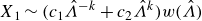 \begin{align} X_1 \sim (c_1\hat \Lambda ^{-k}+c_2\hat \Lambda ^{k})w(\hat \Lambda ) \end{align}
as $\hat \Lambda \rightarrow 0$
, where
$\hat \Lambda \rightarrow 0$
, where $w$
is a function that is at most logarithmically singular at the origin and
$w$
is a function that is at most logarithmically singular at the origin and $c_1$
and
$c_1$
and $c_2$
are arbitrary constants. This reflects a singularity at the origin, which is strongest for large wavenumbers
$c_2$
are arbitrary constants. This reflects a singularity at the origin, which is strongest for large wavenumbers $k$
. For the purpose of resolving this singularity for all
$k$
. For the purpose of resolving this singularity for all $k$
in our computations, we use the transformation
$k$
in our computations, we use the transformation
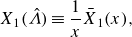 \begin{align} X_1(\hat \Lambda ) \equiv \frac {1}{x} \bar {X}_1(x), \end{align}
where $x = \hat \Lambda ^k$
, within the two-layer region, and solve for
$x = \hat \Lambda ^k$
, within the two-layer region, and solve for $\bar {X}_1$
numerically as a function of
$\bar {X}_1$
numerically as a function of $x$
.
$x$
.
As the problem is $2\pi$
-periodic in the azimuthal direction, only integer values of
$2\pi$
-periodic in the azimuthal direction, only integer values of $k$
are permitted. However, we interpolate for intermediate values of
$k$
are permitted. However, we interpolate for intermediate values of $k$
for illustrative purposes in displaying the results.
$k$
for illustrative purposes in displaying the results.
Given a value of the wavenumber $k$
, the system admits non-zero solutions for specific growth rates, or eigenvalues,
$k$
, the system admits non-zero solutions for specific growth rates, or eigenvalues, $\sigma$
. To find such solutions, we designed an algorithm by exploiting the linearity of the governing equations and boundary conditions. In particular, for a given wavenumber and set of parameter values, we set a guess for the growth rate and shoot backwards as described earlier. In doing so, we obtain two test solutions, denoted by
$\sigma$
. To find such solutions, we designed an algorithm by exploiting the linearity of the governing equations and boundary conditions. In particular, for a given wavenumber and set of parameter values, we set a guess for the growth rate and shoot backwards as described earlier. In doing so, we obtain two test solutions, denoted by $s_1$
and
$s_1$
and $s_2$
, where
$s_2$
, where $s_1$
is calculated by setting
$s_1$
is calculated by setting $\xi _{N1}=1$
and
$\xi _{N1}=1$
and $Q_{l1}|_{\hat \Lambda =L}=0$
and
$Q_{l1}|_{\hat \Lambda =L}=0$
and $s_2$
is calculated by setting
$s_2$
is calculated by setting $\xi _{N1}=0$
and
$\xi _{N1}=0$
and $Q_{l1}|_{\hat \Lambda =L}=1$
. These two solutions are linearly independent and satisfy the perturbation equations and boundary conditions except for perhaps the source flux conditions at the origin. Owing to the linearity of the system, any linear combination of the two solutions is also a solution.
$Q_{l1}|_{\hat \Lambda =L}=1$
. These two solutions are linearly independent and satisfy the perturbation equations and boundary conditions except for perhaps the source flux conditions at the origin. Owing to the linearity of the system, any linear combination of the two solutions is also a solution.
In order to quantify the departure from the source flux boundary conditions, we define a residual matrix:
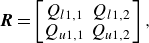 \begin{equation} \boldsymbol{R} = \begin{bmatrix} Q_{l1,1}& Q_{l1,2}\\ Q_{u1,1}& Q_{u1,2} \end{bmatrix}, \end{equation}
where the $i$
th column measures the perturbed source flux at the origin corresponding to the solution
$i$
th column measures the perturbed source flux at the origin corresponding to the solution $s_i$
and
$s_i$
and $i=1,2$
. If the initial guess for the value of the growth rate
$i=1,2$
. If the initial guess for the value of the growth rate $\sigma$
is correct, it is possible to obtain a linear combination of the two test solutions such that the source flux conditions at the origin are satisfied, i.e.
$\sigma$
is correct, it is possible to obtain a linear combination of the two test solutions such that the source flux conditions at the origin are satisfied, i.e. $Q_{l1}=0$
and
$Q_{l1}=0$
and $Q_{u1}=0$
. This is equivalent to
$Q_{u1}=0$
. This is equivalent to $\det (\boldsymbol{R})=0$
, and this particular linear combination is the desired solution to the perturbation equations and all boundary conditions, including the zero source flux boundary conditions. However, if the guessed value of the growth rate is incorrect, then
$\det (\boldsymbol{R})=0$
, and this particular linear combination is the desired solution to the perturbation equations and all boundary conditions, including the zero source flux boundary conditions. However, if the guessed value of the growth rate is incorrect, then $\det (\boldsymbol{R}) \neq 0$
. That is, the growth rate is an admissible eigenvalue if and only if
$\det (\boldsymbol{R}) \neq 0$
. That is, the growth rate is an admissible eigenvalue if and only if $\det (\boldsymbol{R})= 0$
. We, therefore, wish to find values of the growth rate
$\det (\boldsymbol{R})= 0$
. We, therefore, wish to find values of the growth rate $\sigma$
for which
$\sigma$
for which $\det (\boldsymbol{R})= 0$
to within a specified tolerance. In essence, this reduces to a one-dimensional root finding problem for
$\det (\boldsymbol{R})= 0$
to within a specified tolerance. In essence, this reduces to a one-dimensional root finding problem for $\sigma$
.
$\sigma$
.
We note that in order to assess stability, it suffices to consider the eigensolution that corresponds to the largest growth rate, as this gives rise to the most unstable mode. We make sure that our computed solutions for $\sigma$
are largest by manual inspection of plots of the determinant of
$\sigma$
are largest by manual inspection of plots of the determinant of $\boldsymbol{R}$
against the growth rate for a range of test cases. We discuss results, obtained via numerical continuation, in the following section.
$\boldsymbol{R}$
against the growth rate for a range of test cases. We discuss results, obtained via numerical continuation, in the following section.
4. Discussion
In this section, we discuss the onset of instability and relevant characteristics in terms of the growth rates, interval of unstable wavenumbers and the critical wavenumber and how these vary across parameter space. In particular, we map out the behaviour of small disturbances to the base flow in terms of four key dimensionless quantities: the viscosity ratio $\mathcal{M}$
, the density difference
$\mathcal{M}$
, the density difference $\mathcal{D}$
, the total source flux
$\mathcal{D}$
, the total source flux $\mathcal{Q}_u+\mathcal{Q}_l$
and the flux ratio
$\mathcal{Q}_u+\mathcal{Q}_l$
and the flux ratio $\mathcal{Q}_l/\mathcal{Q}_u$
.
$\mathcal{Q}_l/\mathcal{Q}_u$
.
The spatial structure of the perturbation in an unstable configuration is depicted in figure 3 in comparison with the unperturbed base flow. When the intruding layer is perturbed forwards (backwards), it thickens (thins) and protrudes downwards into (recedes upwards from) the lower layer and the lower layer thins (thickens) near the nose. As discussed further in § 4.2, finger growth requires sufficient protrusion of an intruding less viscous fluid downwards into the more viscous underlying layer, rather than upwards into the less viscous air.
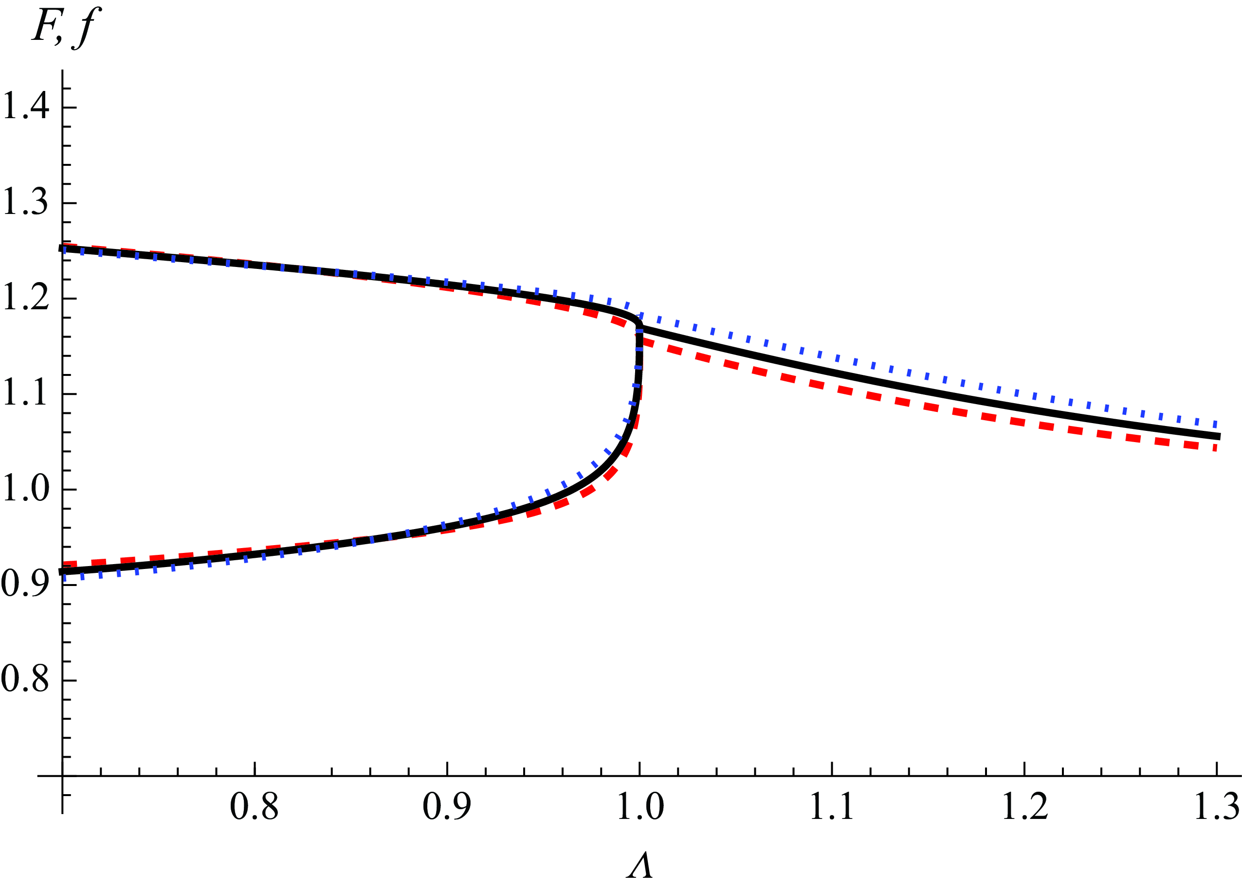
The unperturbed (solid) and perturbed (dashed and dotted) spatial profiles showing the shape of the nose when $k=12$
,
$k=12$
, $\mathcal{M}=200$
,
$\mathcal{M}=200$
, $\mathcal{D}=0.1$
,
$\mathcal{D}=0.1$
, $\mathcal{Q}_u=1$
and
$\mathcal{Q}_u=1$
and $\mathcal{Q}_l=0.2$
. The perturbed profile shown as a dashed (dotted) curve corresponds to intrusions ahead of (behind) the nose of the base flow.
$\mathcal{Q}_l=0.2$
. The perturbed profile shown as a dashed (dotted) curve corresponds to intrusions ahead of (behind) the nose of the base flow.
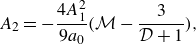
4.1. Thresholds of instability across parameter space
We find that the flow is unstable only for sufficiently large values of the viscosity ratio $\mathcal{M}$
. That is, the intruding layer of viscous fluid needs to be of sufficiently small viscosity for the flow to become unstable. This criterion is similar to what is necessary for the onset of Saffman–Taylor instabilities in porous media, which occur only when the viscosity of the intruding fluid is lower than that of the ambient fluid (Saffman & Taylor Reference Saffman and Taylor1958). Sufficiently large viscosity ratios are also necessary for the onset of fingering instabilities when the less viscous fluid intrudes from below a more viscous gravity current (Kowal & Worster Reference Kowal and Worster2019a
,Reference Kowal and Worster
b
; Leung & Kowal Reference Leung and Kowal2022a
,Reference Leung and Kowal
b
), and when it displaces the more viscous current completely (Kowal Reference Kowal2021). Illustrative values of the viscosity ratio necessary for the onset of instability when the less viscous fluid intrudes from above a more viscous gravity current, as examined in this work, can be seen in figure 4. In particular, figure 4 displays the dispersion relation for the growth rate
$\mathcal{M}$
. That is, the intruding layer of viscous fluid needs to be of sufficiently small viscosity for the flow to become unstable. This criterion is similar to what is necessary for the onset of Saffman–Taylor instabilities in porous media, which occur only when the viscosity of the intruding fluid is lower than that of the ambient fluid (Saffman & Taylor Reference Saffman and Taylor1958). Sufficiently large viscosity ratios are also necessary for the onset of fingering instabilities when the less viscous fluid intrudes from below a more viscous gravity current (Kowal & Worster Reference Kowal and Worster2019a
,Reference Kowal and Worster
b
; Leung & Kowal Reference Leung and Kowal2022a
,Reference Leung and Kowal
b
), and when it displaces the more viscous current completely (Kowal Reference Kowal2021). Illustrative values of the viscosity ratio necessary for the onset of instability when the less viscous fluid intrudes from above a more viscous gravity current, as examined in this work, can be seen in figure 4. In particular, figure 4 displays the dispersion relation for the growth rate $\sigma$
as a function of the wavenumber
$\sigma$
as a function of the wavenumber $k$
, for illustrative parameter values and various values of the viscosity ratio
$k$
, for illustrative parameter values and various values of the viscosity ratio $\mathcal{M}$
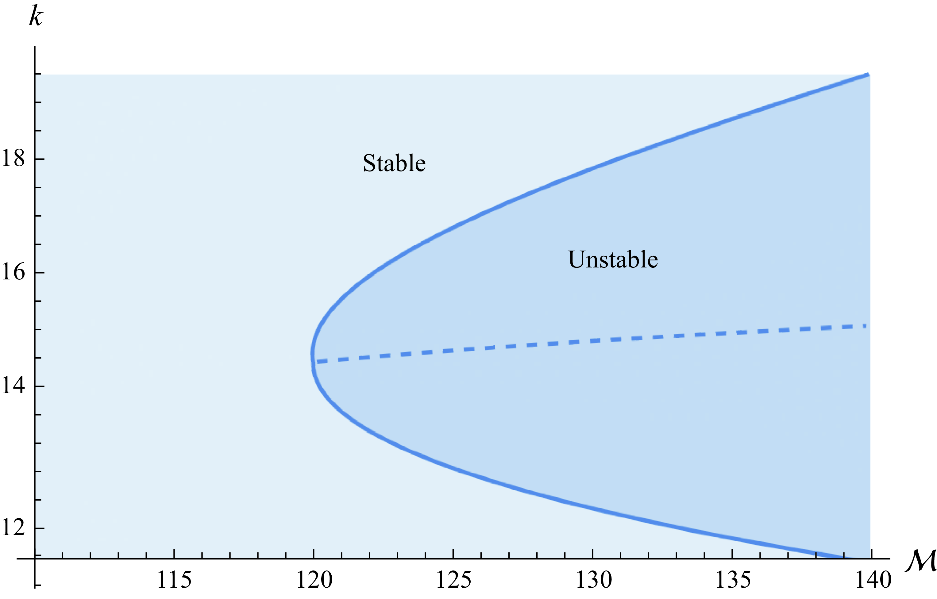
. The growth rate is positive for a bounded interval of wavenumbers only when the viscosity ratio is large enough. That is, the flow is unstable for a bounded interval of wavenumbers only above a critical viscosity ratio. The interval of unstable wavenumbers is shown in figure 5 as a function of the viscosity ratio
$\mathcal{M}$
. The growth rate is positive for a bounded interval of wavenumbers only when the viscosity ratio is large enough. That is, the flow is unstable for a bounded interval of wavenumbers only above a critical viscosity ratio. The interval of unstable wavenumbers is shown in figure 5 as a function of the viscosity ratio $\mathcal{M}$
, where it can be seen that the interval of unstable wavenumbers expands as the viscosity ratio increases. The boundary between the stable and unstable regions, shown in figure 5, depicts the neutral viscosity ratio, defined as the value of the viscosity for which the growth rate is zero. The flow is unstable when the viscosity ratio is above the neutral viscosity ratio. The critical wavenumber
$\mathcal{M}$
, where it can be seen that the interval of unstable wavenumbers expands as the viscosity ratio increases. The boundary between the stable and unstable regions, shown in figure 5, depicts the neutral viscosity ratio, defined as the value of the viscosity for which the growth rate is zero. The flow is unstable when the viscosity ratio is above the neutral viscosity ratio. The critical wavenumber $k_c$
, defined as the wavenumber for which the growth rate is maximal, gradually increases with the wavenumber as depicted in figure 5.
$k_c$
, defined as the wavenumber for which the growth rate is maximal, gradually increases with the wavenumber as depicted in figure 5.
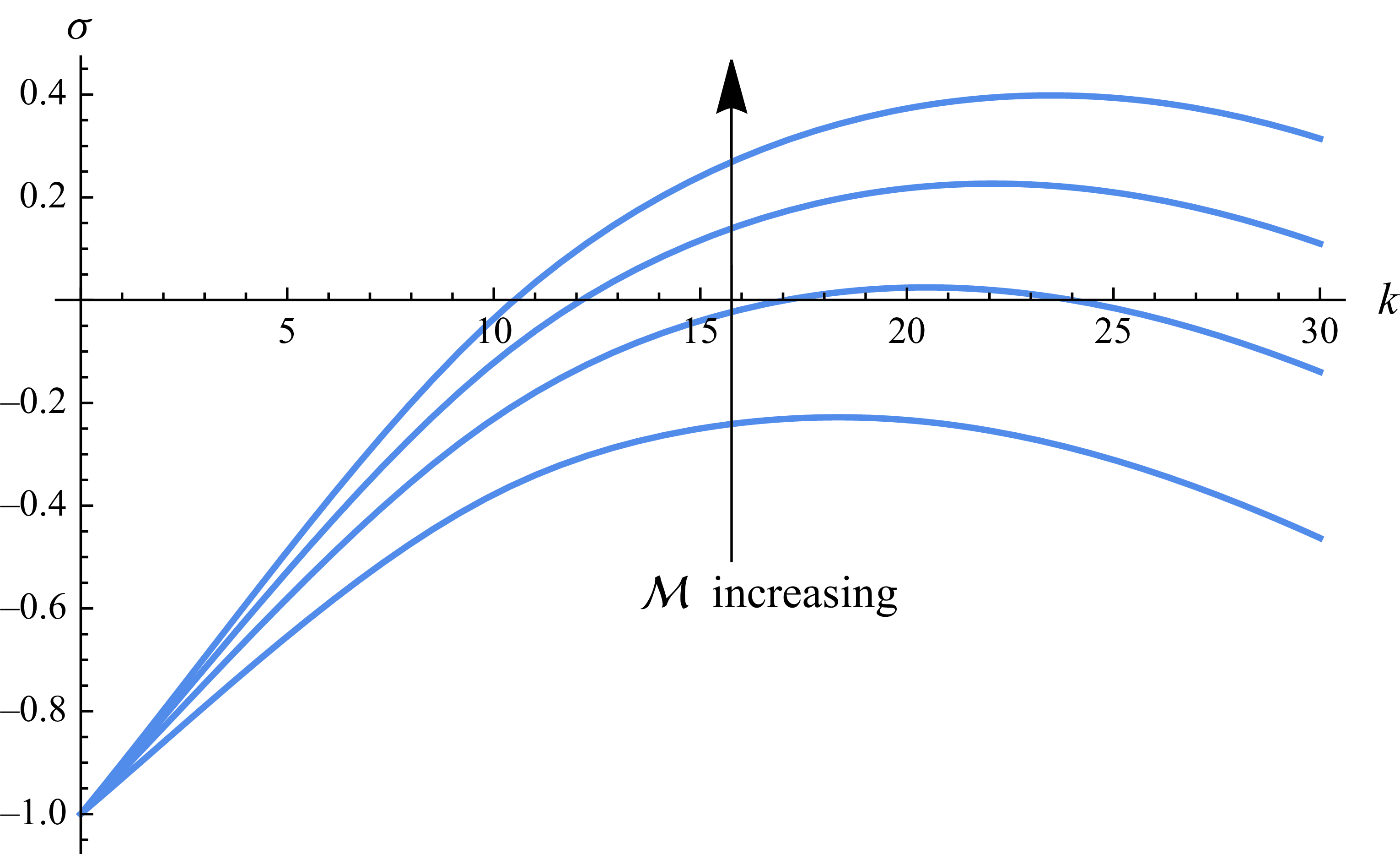
The growth rate versus the wavenumber for various viscosity ratios $\mathcal{M}=20,30,40,50$
when
$\mathcal{M}=20,30,40,50$
when $\mathcal{D}=0.05,\ \mathcal{Q}_u=1$
,
$\mathcal{D}=0.05,\ \mathcal{Q}_u=1$
, $\mathcal{Q}_l = 1$
.
$\mathcal{Q}_l = 1$
.
Neutral stability curve (solid) displaying the interval of unstable wavenumbers as a function of the viscosity ratio, also showing the critical wavenumber $k_c$
(dashed), when
$k_c$
(dashed), when $\mathcal{D}=0.1, \mathcal{Q}_u=1$
and
$\mathcal{D}=0.1, \mathcal{Q}_u=1$
and $\mathcal{Q}_l = 1$
. The flow is unstable (stable) for large (small) viscosity ratios.
$\mathcal{Q}_l = 1$
. The flow is unstable (stable) for large (small) viscosity ratios.
Neutral stability curve (solid) displaying the interval of unstable wavenumbers as a function of the density difference, also showing the critical wavenumber $k_c$
(dashed), when
$k_c$
(dashed), when $\mathcal{M}=120, \mathcal{Q}_u=1$
and
$\mathcal{M}=120, \mathcal{Q}_u=1$
and $\mathcal{Q}_l = 1$
. The flow is unstable (stable) for small (large) density differences.
$\mathcal{Q}_l = 1$
. The flow is unstable (stable) for small (large) density differences.

Contour plot of the maximal growth rate $\sigma _{\textit{max}}$
versus the viscosity ratio
$\sigma _{\textit{max}}$
versus the viscosity ratio $\mathcal{M}$
and density difference
$\mathcal{M}$
and density difference $\mathcal{D}$
, with the neutral stability curve (
$\mathcal{D}$
, with the neutral stability curve ( $\sigma _{\textit{max}}=0$
) displayed as a thick solid curve. The remaining parameter values are
$\sigma _{\textit{max}}=0$
) displayed as a thick solid curve. The remaining parameter values are $\mathcal{Q}_u=1$
and
$\mathcal{Q}_u=1$
and $\mathcal{Q}_l = 1$
. The flow is unstable for high-viscosity ratios and low-density differences.
$\mathcal{Q}_l = 1$
. The flow is unstable for high-viscosity ratios and low-density differences.
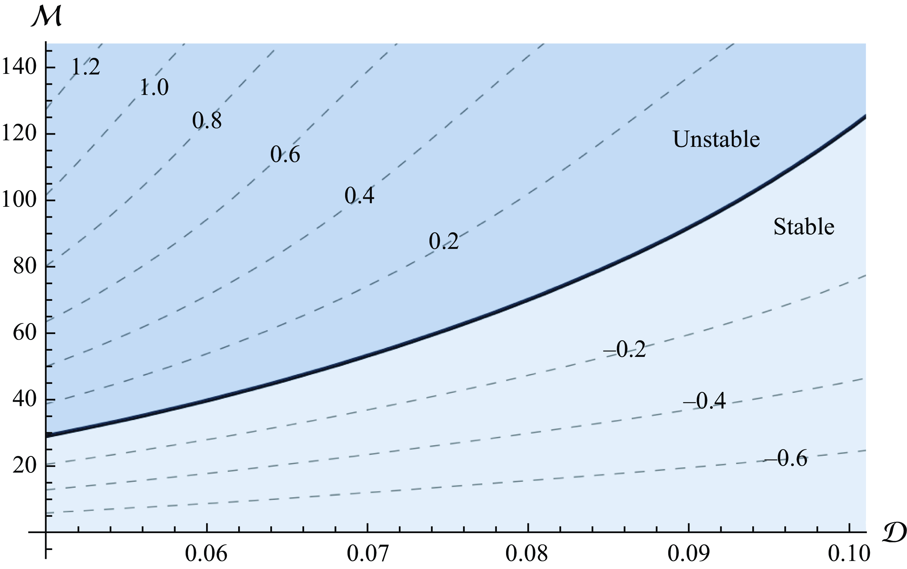
We find that the instability is most profound for low values of the density difference and that it is suppressed completely when the density difference is sufficiently large. This is illustrated in figure 6, depicting an interval of wavenumbers for which the system is unstable below a critical value of the density difference. This interval expands and the critical wavenumber $k_c$
increases as the density difference decreases, as shown in figure 6. Figure 6 also illustrates that the instability is suppressed completely above a critical value of the density difference. This agrees with stability analyses of flows of thin films of viscous fluid intruding underneath another viscous fluid of various rheologies (Kowal & Worster Reference Kowal and Worster2019b
; Leung & Kowal Reference Leung and Kowal2022b
).
$k_c$
increases as the density difference decreases, as shown in figure 6. Figure 6 also illustrates that the instability is suppressed completely above a critical value of the density difference. This agrees with stability analyses of flows of thin films of viscous fluid intruding underneath another viscous fluid of various rheologies (Kowal & Worster Reference Kowal and Worster2019b
; Leung & Kowal Reference Leung and Kowal2022b
).
Neutral stability curve (solid) displaying the interval of unstable wavenumbers as a function of the total source flux, also showing the critical wavenumber $k_c$
(dashed), when
$k_c$
(dashed), when $\mathcal{D}=0.1, \ \mathcal{M}=120$
and
$\mathcal{D}=0.1, \ \mathcal{M}=120$
and $\mathcal{Q}_l/\mathcal{Q}_u = 1$
. The flow is unstable (stable) for large (small) source fluxes.
$\mathcal{Q}_l/\mathcal{Q}_u = 1$
. The flow is unstable (stable) for large (small) source fluxes.

Neutral stability curve (solid) displaying the neutral flux ratio $\mathcal{Q}_l/\mathcal{Q}_u$
as a function of the wavenumber, also showing the critical wavenumber
$\mathcal{Q}_l/\mathcal{Q}_u$
as a function of the wavenumber, also showing the critical wavenumber $k_c$
(dashed), when
$k_c$
(dashed), when $\mathcal{D}=0.1, \ \mathcal{M}=120$
and
$\mathcal{D}=0.1, \ \mathcal{M}=120$
and $\mathcal{Q}_l+\mathcal{Q}_u = 1$
. The flow is unstable for flux ratios above this neutral stability curve.
$\mathcal{Q}_l+\mathcal{Q}_u = 1$
. The flow is unstable for flux ratios above this neutral stability curve.
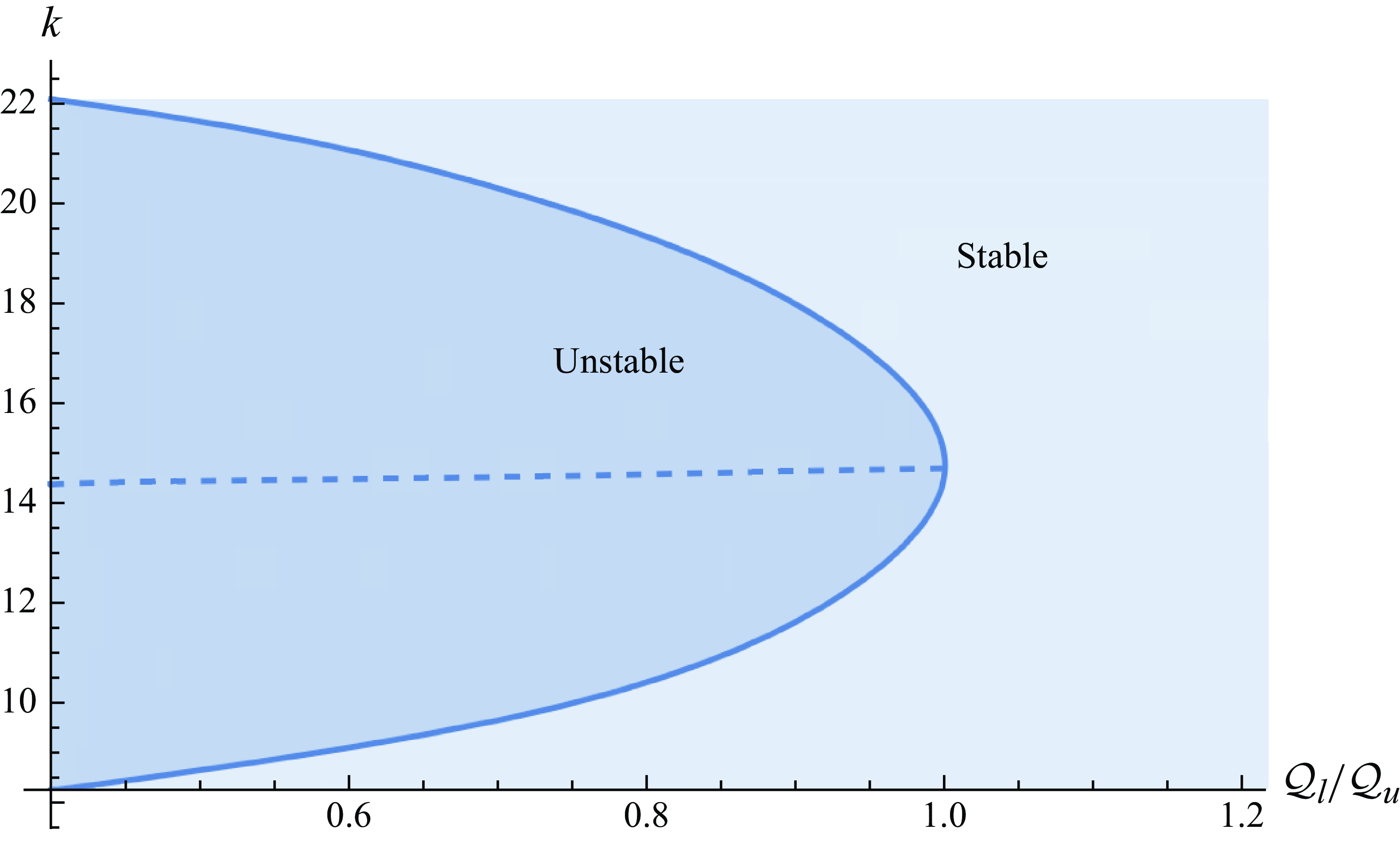
We condense information in the $(\mathcal{M},\mathcal{D})$
-parameter space further in a contour plot of the maximal growth rate
$(\mathcal{M},\mathcal{D})$
-parameter space further in a contour plot of the maximal growth rate $\sigma _{{max}}$
versus the viscosity ratio and density difference, depicted in figure 7. Maximal growth rates are largest for large viscosity ratios and small density differences, with viscosity ratios of the order of 10 required for the onset of instability when the density difference is small. This contrasts with instabilities formed when a free-surface flow is penetrated from below by a less viscous fluid (Kowal & Worster Reference Kowal and Worster2019a
,Reference Kowal and Worster
b
) and with classical Saffman–Taylor instabilities in a Hele-Shaw cell (Saffman & Taylor Reference Saffman and Taylor1958), for which the threshold of instability is of order unity in the viscosity ratio. We discuss why this is to be expected on physical grounds in § 4.2.
$\sigma _{{max}}$
versus the viscosity ratio and density difference, depicted in figure 7. Maximal growth rates are largest for large viscosity ratios and small density differences, with viscosity ratios of the order of 10 required for the onset of instability when the density difference is small. This contrasts with instabilities formed when a free-surface flow is penetrated from below by a less viscous fluid (Kowal & Worster Reference Kowal and Worster2019a
,Reference Kowal and Worster
b
) and with classical Saffman–Taylor instabilities in a Hele-Shaw cell (Saffman & Taylor Reference Saffman and Taylor1958), for which the threshold of instability is of order unity in the viscosity ratio. We discuss why this is to be expected on physical grounds in § 4.2.
We find that the instability is suppressed completely for a sufficiently small total flux $\mathcal{Q}_l+\mathcal{Q}_u$
and sufficiently large flux ratio
$\mathcal{Q}_l+\mathcal{Q}_u$
and sufficiently large flux ratio $\mathcal{Q}_l/\mathcal{Q}_u$
, as depicted in figures 8 and 9. The interval of unstable wavenumbers expands as the total source flux increases and the flux ratio decreases. The critical wavenumber increases with the total source flux and remains approximately constant with respect to the flux ratio. We can therefore expect to see an increasing number of fingers when the total source flux increases, which is consistent with recent experiments in which the intruding fluid is supplied from below (Kumar et al. Reference Kumar, Zuri, Kogan, Gottlieb and Sayag2021).
$\mathcal{Q}_l/\mathcal{Q}_u$
, as depicted in figures 8 and 9. The interval of unstable wavenumbers expands as the total source flux increases and the flux ratio decreases. The critical wavenumber increases with the total source flux and remains approximately constant with respect to the flux ratio. We can therefore expect to see an increasing number of fingers when the total source flux increases, which is consistent with recent experiments in which the intruding fluid is supplied from below (Kumar et al. Reference Kumar, Zuri, Kogan, Gottlieb and Sayag2021).
We condense information further in a contour plot of the maximal growth rate $\sigma _{max}$
versus the total flux and flux ratio, shown in figure 10. As seen in figure 10, growth rates are largest when the total flux is large and a sufficiently large total flux (of order unity) is required for the onset of instability. Equivalently, the onset of instability requires the flux of the upper layer to be sufficiently large relative to that of the lower layer. This is in line with the experiments of Lister & Kerr (Reference Lister and Kerr1989), in which a low-viscosity fluid intrudes at the interface between two other fluids and no instabilities were observed, save for small-scale frontal patterning that the authors attribute to contamination of the fluid surface by dust. These experiments were carried out for dimensionless fluxes in the range
$\sigma _{max}$
versus the total flux and flux ratio, shown in figure 10. As seen in figure 10, growth rates are largest when the total flux is large and a sufficiently large total flux (of order unity) is required for the onset of instability. Equivalently, the onset of instability requires the flux of the upper layer to be sufficiently large relative to that of the lower layer. This is in line with the experiments of Lister & Kerr (Reference Lister and Kerr1989), in which a low-viscosity fluid intrudes at the interface between two other fluids and no instabilities were observed, save for small-scale frontal patterning that the authors attribute to contamination of the fluid surface by dust. These experiments were carried out for dimensionless fluxes in the range $8.7\times 10^{-6}$
–
$8.7\times 10^{-6}$
– $5.3\times 10^{-5}$
, which is much less than the threshold (of order unity) required for instability. The threshold is also consistent with the experiments of Dauck (Reference Dauck2020), for which the dimensionless flux reached up to approximately
$5.3\times 10^{-5}$
, which is much less than the threshold (of order unity) required for instability. The threshold is also consistent with the experiments of Dauck (Reference Dauck2020), for which the dimensionless flux reached up to approximately $160$
and instabilities were observed.
$160$
and instabilities were observed.
The stability thresholds discussed in this section are summarised in the most condensed contour plot shown in figure 11, displaying the critical total flux required for the onset of instability in $(\mathcal{D},\mathcal{M})$
space for various values of the flux ratio. Values of the critical viscosity ratio and critical density difference required for the onset of instability can be read off from figure 11. Alternatively, figure 11 can be interpreted as a plot of the critical viscosity ratio versus the density difference for various values of the total flux and flux ratio. The higher the total flux, the lower the viscosity ratio required for the onset of instability, and the larger the interval of density differences for which instabilities appear.
$(\mathcal{D},\mathcal{M})$
space for various values of the flux ratio. Values of the critical viscosity ratio and critical density difference required for the onset of instability can be read off from figure 11. Alternatively, figure 11 can be interpreted as a plot of the critical viscosity ratio versus the density difference for various values of the total flux and flux ratio. The higher the total flux, the lower the viscosity ratio required for the onset of instability, and the larger the interval of density differences for which instabilities appear.
Contour plot of the maximal growth rate $\sigma _{{max}}$
versus the flux ratio
$\sigma _{{max}}$
versus the flux ratio $\mathcal{Q}_l/\mathcal{Q}_u$
and total flux
$\mathcal{Q}_l/\mathcal{Q}_u$
and total flux $\mathcal{Q}_l+\mathcal{Q}_u$
, with the neutral stability curve (
$\mathcal{Q}_l+\mathcal{Q}_u$
, with the neutral stability curve ( $\sigma _{{max}}=0$
) displayed as a thick solid curve. The remaining parameter values are
$\sigma _{{max}}=0$
) displayed as a thick solid curve. The remaining parameter values are $\mathcal{M}=120$
and
$\mathcal{M}=120$
and $\mathcal{D} = 0.1$
. The flow is unstable when the total flux is large and flux ratio is small.
$\mathcal{D} = 0.1$
. The flow is unstable when the total flux is large and flux ratio is small.
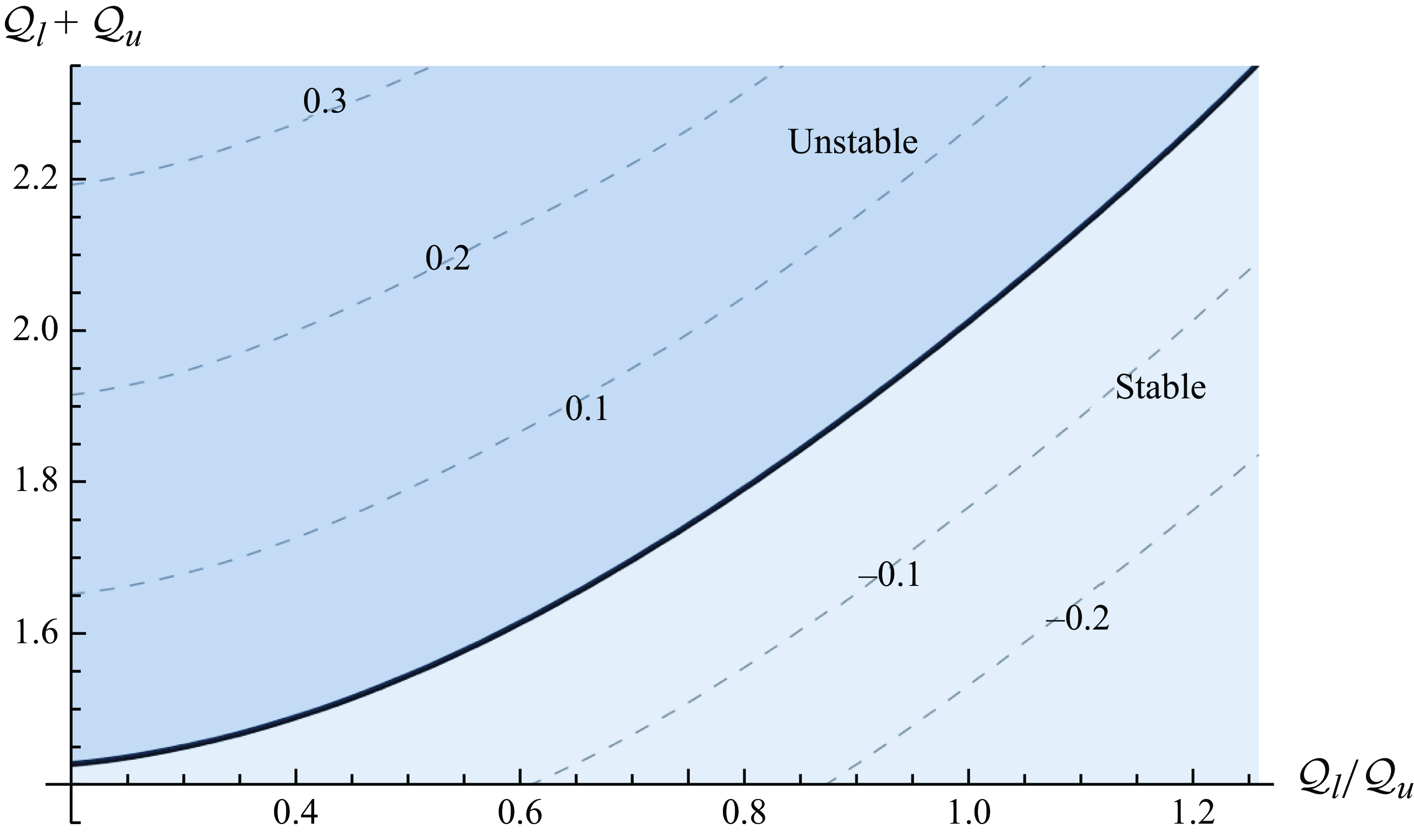
Contour plot of the critical total flux $\mathcal{Q}_l+\mathcal{Q}_u$
required for the onset of instability in
$\mathcal{Q}_l+\mathcal{Q}_u$
required for the onset of instability in $(\mathcal{D},\mathcal{M})$
space when
$(\mathcal{D},\mathcal{M})$
space when $\mathcal{Q}_l/\mathcal{Q}_u=0.4$
(solid curves), 0.5 (dashed curves) and 0.6 (dotted curves).
$\mathcal{Q}_l/\mathcal{Q}_u=0.4$
(solid curves), 0.5 (dashed curves) and 0.6 (dotted curves).
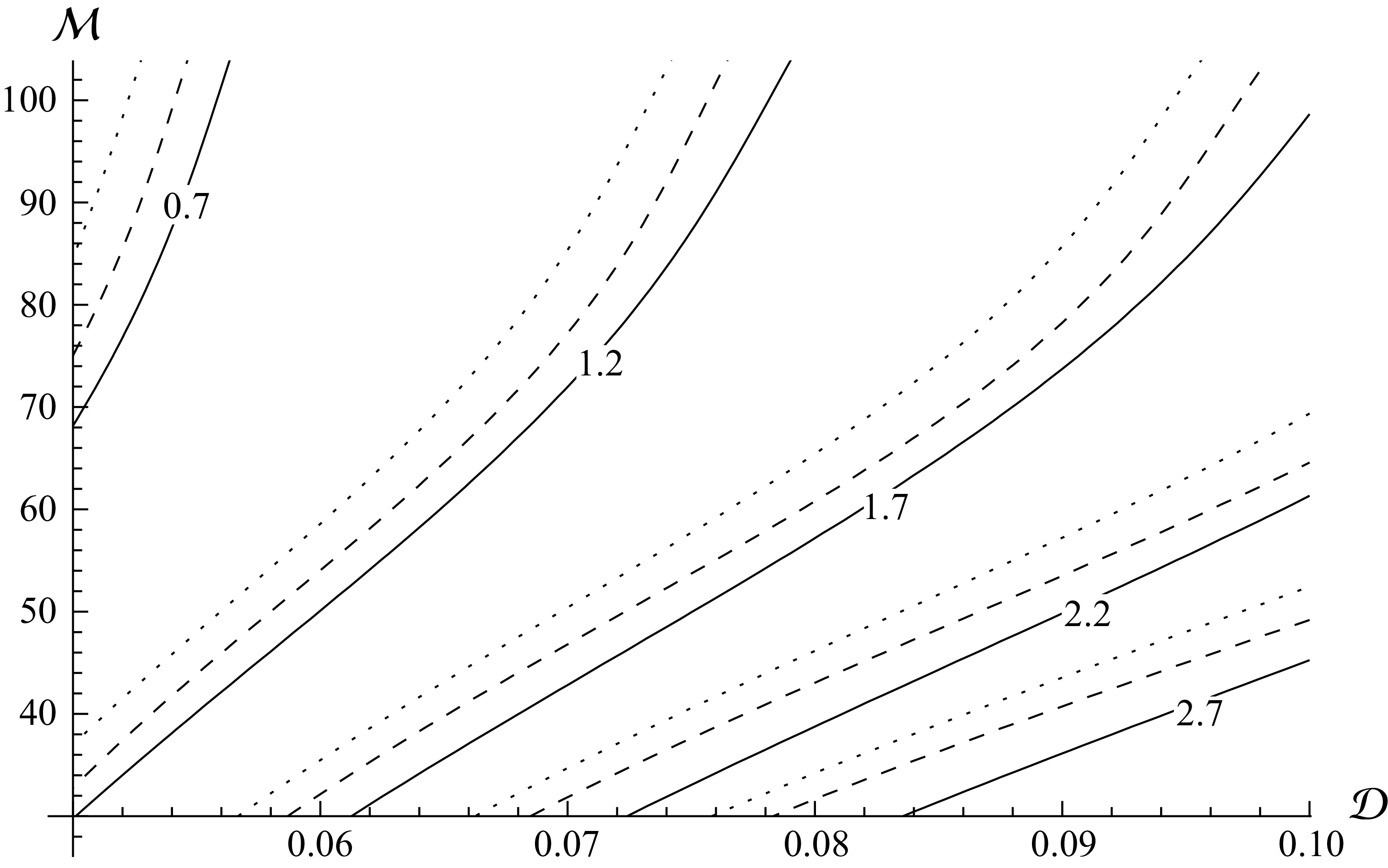
4.2. Mechanism of instability and suppression
To understand the mechanism of instability physically, it is instructive to compare with classical viscous fingering in porous-media/Hele-Shaw cells. The mechanisms of instability are similar in that there is less flow resistance along the fingers of a less viscous fluid than in the gaps between them filled with a more viscous fluid, thus resulting in the fingers growing (when the intruding fluid is less viscous than the ambient). However, in the free-surface case examined here, the intruding fluid is also advancing into atmosphere (which is less viscous, so the viscosity contrast is stabilising), so finger growth is reliant on the intruding fingers displacing the lubricating liquid ‘more’ than displacing the atmosphere. In other words, finger growth requires the density difference $\mathcal{D}$
to be sufficiently small (as seen in figure 6) and the upper-layer flux
$\mathcal{D}$
to be sufficiently small (as seen in figure 6) and the upper-layer flux $\mathcal{Q}_u$
to be sufficiently large relative to the lower-layer flux
$\mathcal{Q}_u$
to be sufficiently large relative to the lower-layer flux $\mathcal{Q}_l$
and relative to unity (as seen in figures 8–10) that the fingers can sink down into rather than just riding on top of the lubricating layer.
$\mathcal{Q}_l$
and relative to unity (as seen in figures 8–10) that the fingers can sink down into rather than just riding on top of the lubricating layer.
In contrast, when the less viscous fluid intrudes beneath another thin film of viscous fluid (the set-up of Kowal & Worster Reference Kowal and Worster2019a ,Reference Kowal and Worster b ), it is not stabilised by its advance into a less viscous atmosphere and so the instability thresholds are lower than reported here. In particular, the critical viscosity ratio required for the onset of instability in the set-up of Kowal & Worster (Reference Kowal and Worster2019a ,Reference Kowal and Worster b ) is of order unity when the intruding layer is supplied from below, which is one to two orders of magnitude smaller than when the less viscous fluid intrudes from above as in the current work. However, the general trends in the stability thresholds are qualitatively similar as the parameters vary. For example, for both systems, there is a critical density difference above which the instabilities are compressed, with the interval of unstable wavenumbers widening as the density difference decreases. The critical density difference is of order unity (versus one tenth) when the less viscous fluid intrudes from below (versus above).
To explore the mechanism of suppression further, it is also instructive to focus on contributions that are significant for large density differences. Non-zero density differences between the two layers of viscous fluid give rise to additional buoyancy forces within the lower layer near the front of the intruding fluid. These are associated with the gravitational spreading of the underlying layer under its own weight, dragging the upper layer along with it. As gradients of the lower-layer thickness are positive near the front when the density difference is non-zero, the contributions to the flow velocity, arising from the spreading of the lower layer under its own weight, are negative within the underlying layer. This, in turn, induces an inwards contribution to the flow, seen most clearly in the velocity profiles of figure 5 of Yang et al. (Reference Yang, Mottram and Kowal2024). That is, in what would have been an unstable configuration, this contribution involves a more viscous fluid intruding (inwards) into a less viscous fluid, which is stabilising.
Similar buoyancy forces stabilise the flow of single-layer viscous gravity currents, where a viscous fluid intrudes into air (less viscous) – a stable viscosity contrast (Mathunjwa & Hogg Reference Mathunjwa and Hogg2006). Small perturbations to single-layer viscous gravity currents, which are driven by buoyancy forces alone, have been found to decay and the flow has been found to approach a similarity solution at late times (Mathunjwa & Hogg Reference Mathunjwa and Hogg2006; Ball & Huppert Reference Ball and Huppert2019). For two-layer flows, these buoyancy forces contribute to the flow only when the densities of the two viscous fluids are unequal. When the density difference increases, so does the effect of these buoyancy forces, especially near the front, where they are most profound as depicted in figure 5 of Yang et al. (Reference Yang, Mottram and Kowal2024). As the instability is a frontal instability, the dynamics near the front, and particularly the effect of these buoyancy forces, is what determines the onset of instability, and hence it is natural to expect these forces to have a stabilising effect when the density difference is sufficiently large, as seen in figure 6.
5. Conclusions
In this work, we have demonstrated that a free-surface flow consisting of a thin film of viscous fluid intruding over another layer of fluid of dissimilar viscosity and density is prone to a new type fingering instability, termed the non-porous viscous fingering instability. This type of instability is most closely related to Saffman–Taylor viscous fingering in a porous medium or a Hele-Shaw cell, but this time without a porous medium or Hele-Shaw cell present. The similarity between these two types of instability is that a viscosity contrast between two fluids is needed for both instabilities to occur. The difference between them is that the jump in pressure gradient driving the instabilities is hydrostatic for the former and dynamic for the latter form of instability.
We also point out features distinguishing the non-porous viscous fingering instability from other frontal instabilities, including the fingering of a driven spreading film and thermoviscous fingering. We found that a free-surface flow of a low-viscosity fluid is more prone to instability when intruding into a high-viscosity fluid from below (as in Kowal & Worster Reference Kowal and Worster2019a ,Reference Kowal and Worster b ) than from above (as in the present paper). Intuitively, this is because the less viscous fluid also displaces the atmosphere (an even less viscous fluid) in the latter scenario, which is stabilising.
We have also examined the stabilising influence of buoyancy forces, which form near the nose of a thin film of viscous fluid as it intrudes into another viscous fluid of different density and viscosity. These buoyancy forces are greatest near the front of the intruding layer and feature as the only physical mechanism driving the flow of single-layer viscous gravity currents, for example. Such buoyancy forces have been shown to be stabilising for single-layer flows (Grundy & McLaughlin Reference Grundy and McLaughlin1982; Mathunjwa & Hogg Reference Mathunjwa and Hogg2006) and for two-phase flows, when the intruding layer is supplied from below (Kowal & Worster Reference Kowal and Worster2019a ,Reference Kowal and Worster b ) or when it completely displaces the ambient layer (Kowal Reference Kowal2021).
We found that a sufficiently large viscosity ratio is required in order for the instability to occur, and that the instability is suppressed completely for large enough density differences between the two layers. For large enough density differences, driving buoyancy forces associated with the gravitational spreading of the lubricating layer under its own weight become more pronounced, and stabilise the flow completely. For lower density differences, for which the system is unstable, this mechanism provides for wavelength selection, stabilising the flow for large wavenumbers in contrast to intermediate wavenumbers. This indicates that the hydrodynamic interactions of the two layers of viscous fluid alone suffice in stabilising the flow for large wavenumbers, giving rise to wavelength selection. This contrasts with classical Saffman–Taylor viscous fingering, which is instead stabilised by other mechanisms, such as the effects of surface tension or fluid mixing, for example. Such effects, however, may further stabilise the flow considered in this work, likely leading to smaller growth rates for large wavenumbers and smaller critical wavenumbers.
We also found evidence of the role of the source flux in the onset of these fingering instabilities. In particular, the flow is unstable only when the source flux of the upper layer is large enough relative to that of the lower layer, which is consistent with available experimental observations when the intruding fluid is supplied from below, for various rheologies, and from above.
Our observations may shed light on the appearance and possible suppression mechanisms of similar fingering instabilities found in nature and industry at various length and time scales, modulo the influence of secondary effects such as surface tension, or fluid mixing, for instance. Examples include drug-mucus interactions in nasal drug/vaccine delivery, the manufacture of patterned substrates and the interaction of dissimilar lava flows, for example.
Acknowledgements
We would like to thank N.J. Mottram for insightful discussions.
Funding
H.Y. acknowledges the support of an EPSRC studentship. K.N.K. acknowledges the support of EPSRC grant EP/Y021959/1.
Declaration of interests
The authors report no conflict of interest.
Data availability statement
The data that support the findings of this study are directly available within this publication.
Appendix A. Asymptotic expansions near the intrusion front
Similar to the base flows of Yang et al. (Reference Yang, Mottram and Kowal2024), we find that the thicknesses of the two layers can be expanded as
 \begin{equation} \begin{aligned} F(\xi ,\vartheta ,\tau ) &\sim A_1(\vartheta ,\tau )\delta ^{\frac {1}{2}}+A_2(\vartheta ,\tau )\delta +A_3(\vartheta ,\tau )\delta ^{\frac {3}{2}}\ldots , \\ f(\xi ,\vartheta ,\tau ) &\sim a_0(\vartheta ,\tau )+a_1(\vartheta ,\tau )\delta ^{\frac {1}{2}}+a_2(\vartheta ,\tau )\delta +a_3(\vartheta ,\tau )\delta ^{\frac {3}{2}}\ldots . \end{aligned} \end{equation}
near the intrusion front where $\delta =(1-\xi /\xi _N)\ll 1$
.
$\delta =(1-\xi /\xi _N)\ll 1$
.
For the governing equation (3.7) describing the lower layer, the leading-order contribution is of $O(\delta ^{-3/2})$
and yields the relationship
$O(\delta ^{-3/2})$
and yields the relationship
 \begin{equation} (\mathcal{D}+1)a_1+A_1=0 \end{equation}
between $A _1$
and
$A _1$
and $a_1$
. The leading-order contribution of the governing equation (3.6) for the upper layer is of
$a_1$
. The leading-order contribution of the governing equation (3.6) for the upper layer is of $O(\delta ^{-1/2})$
and gives rise to
$O(\delta ^{-1/2})$
and gives rise to
 \begin{equation} (\mathcal{D}+1)a_2+A_2+\frac {A_1^2 \mathcal{D}}{a_0 (\mathcal{D}+1)}-\frac {\xi _N^2}{3 a_0^2}-\frac {2\xi _N}{3a_0^2}{\frac {\partial \xi _N}{\partial \tau }}+O\left ({\frac {\partial }{\partial \vartheta }}\times {\frac {\partial }{\partial \vartheta }}\right )=0, \end{equation}
where $O ({({\partial }/{\partial \vartheta })}\times {({\partial }/{\partial \vartheta })} )$
represent terms that contain products of two azimuthal derivatives, which are zero for the base solution and negligible for small-amplitude perturbations. This equation is identical to the equivalent equation for the base flow apart from the addition of the term containing a derivative with respect to
$O ({({\partial }/{\partial \vartheta })}\times {({\partial }/{\partial \vartheta })} )$
represent terms that contain products of two azimuthal derivatives, which are zero for the base solution and negligible for small-amplitude perturbations. This equation is identical to the equivalent equation for the base flow apart from the addition of the term containing a derivative with respect to $\tau$
and the (negligible) higher-order terms.
$\tau$
and the (negligible) higher-order terms.
Going to the next order, the $O (\delta ^{-{1}/{2}} )$
contribution to (3.7) and the
$O (\delta ^{-{1}/{2}} )$
contribution to (3.7) and the $O(1)$
contribution to (3.6) yield
$O(1)$
contribution to (3.6) yield
 \begin{align} (\mathcal{D}+1)a_3+A_3+\gamma _1+O\left ({\frac {\partial }{\partial \vartheta }}\times {\frac {\partial }{\partial \vartheta }}\right )=0,& \end{align}
 \begin{align} (\mathcal{D}+1)a_3+A_3+\gamma _2+O\left ({\frac {\partial }{\partial \vartheta }}\times {\frac {\partial }{\partial \vartheta }}\right )=0,& \end{align}
respectively, where
 \begin{equation} \gamma _1=-\frac {A_1^3 \mathcal{D}}{a_0^2 (\mathcal{D}+1)^2}-\frac {A_2 A_1 (2-3 \mathcal{D})}{2 a_0 (\mathcal{D}+1)}+\frac {A_1 \xi _N^2}{3 a_0^3 (\mathcal{D}+1)}-\frac {a_2 A_1}{a_0}+\frac {2A_1\xi _N}{3a_0^3(1+\mathcal{D})}{\frac {\partial \xi _N}{\partial \tau }}, \end{equation}
and
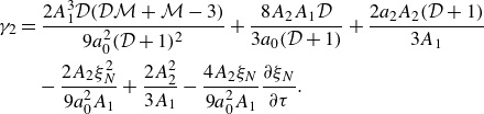 \begin{align} \gamma _2&=\frac {2 A_1^3 \mathcal{D} (\mathcal{D} \mathcal{M}+\mathcal{M}-3)}{9 a_0^2 (\mathcal{D}+1)^2}+\frac {8 A_2 A_1 \mathcal{D}}{3 a_0( \mathcal{D}+1)}+\frac {2 a_2 A_2 (\mathcal{D}+1)}{3 A_1}\nonumber \\&\quad -\frac {2 A_2 \xi _N^2}{9 a_0^2 A_1}+\frac {2 A_2^2}{3 A_1}-\frac {4A_2\xi _N}{9a_0^2A_1}{\frac {\partial \xi _N}{\partial \tau }}. \end{align}
Similarly to before, these coefficients generalise those describing the base flow through the addition of terms involving derivatives with respect to $\tau$
and the higher-order terms. We note that (A4) and (A5) depend on
$\tau$
and the higher-order terms. We note that (A4) and (A5) depend on $A_3$
and
$A_3$
and $a_3$
through the combination
$a_3$
through the combination $(D+1)a_3 + A_3$
, which can be eliminated by subtracting (A4) from (A5), which gives
$(D+1)a_3 + A_3$
, which can be eliminated by subtracting (A4) from (A5), which gives
 \begin{align} \gamma _1=\gamma _2. \end{align}
Finally, solving (A3) and (A8) for $A_2$
and
$A_2$
and $a_2$
yields
$a_2$
yields
 \begin{align}&\qquad\qquad\qquad\qquad\quad A_2 = -\frac {4A_1^2}{9 a_0}\left (\mathcal{M}-\frac {3}{\mathcal{D}+1}\right ), \end{align}
 \begin{align}& a_2 = \frac {1}{9 (\mathcal{D}+1) a_0^2 }\left [3 \xi _N \left (\xi _N+2 \frac {\partial \xi _N}{\partial \tau } \right ) + A_1^2 a_0 \left ( 4 \mathcal{M}-9-\frac {3}{\mathcal{D}+1}\right ) \right ], \end{align}
specifying $a_2$
and
$a_2$
and $A_2$
in terms of
$A_2$
in terms of $a_0$
,
$a_0$
, $A_1$
and
$A_1$
and $\xi _N$
.
$\xi _N$
.
Appendix B. Perturbed fluxes
Explicit expressions for perturbations to the fluxes are given by (3.27)–(3.30), where
 \begin{align}&\qquad\qquad\quad\,\, \alpha _{u1} = -\frac {3}{\xi _{N0}} F_0 \left [f_0 \left ((\mathcal{D}+1) f_0'+F_0'\right )+F_0 \left (f_0'+F_0'\right )\right ], \end{align}
 \begin{align}&\,\, \alpha _{u2}=-\frac {3}{2 \xi _{N0}} \left [f_0^2 \left ((\mathcal{D}+1) f_0'+F_0'\right )+2\mathcal{M} F_0^2 \left (f_0'+F_0'\right )+4 f_0 F_0 \left (f_0'+F_0'\right )\right ], \end{align}
 \begin{align}&\qquad\qquad\qquad\quad \alpha _{u3}=-\frac {1}{2 \xi _{N0}}F_0 \left [3 (\mathcal{D}+1) f_0^2+6 f_0 F_0+2\mathcal{M} F_0^2 \right ], \end{align}
 \begin{align}&\qquad\qquad\qquad\qquad\,\, \alpha _{u4}=-\frac {1}{2 \xi _{N0}}F_0 \left [6 f_0 F_0+3 f_0^2+2\mathcal{M} F_0^2 \right ], \end{align}
 \begin{align}& \alpha _{u5}=\frac {1}{2 \xi _{N0}^2}F_0 \left [3 f_0^2 \left ((\mathcal{D}+1) f_0'+F_0'\right )+2 \mathcal{M}F_0^2 \left (f_0'+F_0'\right )+6 f_0 F_0 \left (f_0'+F_0'\right )\right ], \end{align}
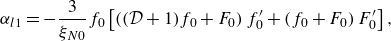 \begin{align}&\qquad\qquad\qquad \alpha _{l1} = -\frac {3}{\xi _{N0}} f_0 \left [ \left ((\mathcal{D}+1) f_0+F_0\right )f_0'+\left (f_0+F_0\right ) F_0'\right ], \end{align}
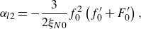 \begin{align}&\qquad\qquad\qquad\qquad\qquad\qquad\, \alpha _{l2} =-\frac {3}{2 \xi _{N0}} f_0^2 \left (f_0'+F_0'\right ), \end{align}
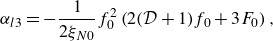 \begin{align}&\qquad\qquad\qquad\qquad\qquad\,\, \alpha _{l3} =-\frac {1}{2 \xi _{N0}}f_0^2 \left (2 (\mathcal{D}+1) f_0+3 F_0\right ), \end{align}
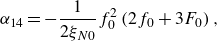 \begin{align}&\qquad\qquad\qquad\qquad\qquad\qquad \alpha _{14}=-\frac {1}{2 \xi _{N0}}f_0^2 \left (2 f_0+3 F_0\right ), \end{align}
 \begin{align}&\qquad\qquad\quad\,\, \alpha _{l5}=\frac {1}{2 \xi _{N0}^2}f_0^2 \left [2 f_0 \left ((\mathcal{D}+1) f_0'+F_0'\right )+3 F_0 \left (f_0'+F_0'\right )\right ]. \end{align}


 Open access