







1. Introduction
The theoretical and experimental study of the unsteady dynamics of gravitational plane liquid sheets (curtains) issuing from a vertical slot has interested the scientific community for decades (Finnicum, Weinstein & Rushak Reference Finnicum, Weinstein and Rushak1993; Clarke et al. Reference Clarke, Weinstein, Moon and Simister1997; Weinstein et al. Reference Weinstein, Clarke, Moon and Simister1997; Lin Reference Lin2003; Barlow, Weinstein & Helenbrook Reference Barlow, Weinstein and Helenbrook2012). Nowadays, further insights can be provided by direct numerical simulation of the relevant two-phase flow field (Della Pia, Chiatto & de Luca Reference Della Pia, Chiatto and de Luca2020), which enables the solution of the curtain motion and of the surrounding gaseous ambient to be predicted simultaneously. The free and forced dynamic responses of such a flow system have been investigated for the cases of sheet interacting with a one-sided air cushion (nappe configuration, Binnie Reference Binnie1974; Sato et al. Reference Sato, Miura, Nagamine, Morii and Ohkubo2007; Girfoglio et al. Reference Girfoglio, De Rosa, Coppola and de Luca2017; Lodomez et al. Reference Lodomez, Pirotton, Dewals, Archambeau and Erpicum2018; Kitsikoudis et al. Reference Kitsikoudis, Lodomez, Dewals, Archambeau, Pirotton and Erpicum2021) and unconfined gaseous ambient (Schmidt & Oberleithner Reference Schmidt and Oberleithner2020; Della Pia, Chiatto & de Luca Reference Della Pia, Chiatto and de Luca2021; Torsey et al. Reference Torsey, Weinstein, Ross and Barlow2021), both in supercritical ( $We > 1$) and subcritical ( $We < 1$) regimes. The Weber number $We$ is here defined as the ratio between inertia and capillary forces, $We = \rho _l U^{\star 2}_{in} H^{\star }_{in}/(2 \sigma )$, with $\rho _l$ and $\sigma$ being the liquid density and the surface tension coefficient, $U^{\star }_{in}$ and $H^{\star }_{in}$ the liquid velocity and curtain thickness at the slot exit section, respectively.
Despite the historical and the more recent efforts, several unanswered questions remain regarding the unsteady dynamics of liquid curtains; among others, the physical mechanisms leading to the sheet break-up in subcritical conditions are still unclear. From one hand, theoretical and experimental works point out that a necessary condition for the stability of thin two-dimensional liquid curtains issuing from a slot and falling vertically under the influence of gravity is  $We > 1$ (Brown Reference Brown1961; Lin Reference Lin1981; Lin & Roberts Reference Lin and Roberts1981); from the other hand, the experimental investigations carried out by Finnicum et al. (Reference Finnicum, Weinstein and Rushak1993) revealed that stable liquid curtains can exist under a wide range of flow conditions, spanning both the supercritical and subcritical regimes ( $0.02< We < 2$). From the literature analysis summarized above, it can be inferred that an interesting open question concerns the sheet unsteady behaviour when the flow rate is reduced and the Weber number traverses the critical threshold ( $We=1$). The topic is important from the technological aspect because two-dimensional planar liquid sheets, falling under the influence of gravity, are often employed to deposit liquid layers on a solid moving surface during coating processes (Finnicum et al. Reference Finnicum, Weinstein and Rushak1993; Weinstein & Ruschak Reference Weinstein and Ruschak2004), and can be subjected to ambient disturbances that cause non-uniform coating layers.
It is known that the prevailing flow disturbances characterizing the dynamics of gravitational planar liquid sheets are represented by travelling waves with velocity  $\pm \sqrt {U/We}$ relative to that of the base flow $U$ (Weinstein et al. Reference Weinstein, Clarke, Moon and Simister1997); therefore, in the supercritical regime ( $We>1$) all perturbations travel downstream along the curtain, being faster than the underlying base flow, while for $We < 1$ there exist upstream travelling disturbances which affect the curtain centreline slope at the slot exit section, whose specific value depends on the (subcritical) Weber number. Focusing on the flow transition from the supercritical to subcritical regime, the recent numerical investigation by Della Pia et al. (Reference Della Pia, Chiatto and de Luca2021), who provided a simplified one-dimensional model of the dynamics of a sheet of finite length accounting for the coupling between the curtain motion and the surrounding gaseous environment, highlighted the discontinuity (jump) of the flow natural frequency when the Weber number reduces below the critical threshold $We=1$. On the other hand, Torsey et al. (Reference Torsey, Weinstein, Ross and Barlow2021), who studied the case of forced (rather than natural) dynamic response of an infinite curtain subjected to sinusoidal ambient pressure disturbances not coupled with the curtain motion, did not find any discontinuity in interface shape and amplitude, and they hypothesized this behaviour could be related to the modelling of the sheet–ambient interaction considered in a finite length curtain that bounds a finite and enclosed air region.
The motivation of the present paper is twofold. On the one hand, it will be shown that the curtain forced response to sinusoidal transverse velocity perturbations is continuous across the critical threshold  $We=1$, not depending on the particular model of sheet–ambient interaction. On the other hand, experimental evidence of the discontinuous behaviour of the curtain natural response in transcritical conditions will be provided, which can be numerically predicted through a Bernoulli based model of sheet–ambient interaction for a finite length sheet. Although several previous contributions reported on measurements of the natural frequency of liquid sheet flows, such as the historical work of Binnie (Reference Binnie1974) and more recent papers by Sato et al. (Reference Sato, Miura, Nagamine, Morii and Ohkubo2007), Lodomez et al. (Reference Lodomez, Pirotton, Dewals, Archambeau and Erpicum2018, Reference Lodomez, Crookston, Tullis and Erpicum2019a,Reference Lodomez, Tullis, Dewals, Archambeau, Pirotton and Erpicumb, Reference Lodomez, Tullis, Archambeau, Kitsikoudis, Pirotton, Dewals and Erpicum2020) and Kitsikoudis et al. (Reference Kitsikoudis, Lodomez, Dewals, Archambeau, Pirotton and Erpicum2021) regarding the nappe configuration, to the authors’ knowledge this is the first time that the experimental occurrence of the frequency jump of an unconfined liquid curtain in transcritical conditions is provided.
The work is organized as follows: in § 2, the theoretical and numerical framework is introduced; § 3 highlights the experimental method employed in the analysis, together with a description of the apparatus used to generate the vertical liquid curtain; results are presented and discussed in § 4, and conclusions are drawn in § 5. Finally, further theoretical and numerical insights into both the natural and forced liquid sheet dynamics are provided in Appendices A and B.
2. Theoretical and numerical modelling
Both the natural and forced responses of a gravitational liquid sheet, interacting with an unconfined gaseous ambient, are analysed by means of a linear inviscid one-dimensional model, described in detail in previous contributions (Della Pia et al. Reference Della Pia, Chiatto and de Luca2020, Reference Della Pia, Chiatto and de Luca2021). Despite the simplifying assumptions, the predictions of this model were found to be valuable compared with two-phase numerical simulations carried out with a volume-of-fluid (VOF) code (Popinet Reference Popinet2003, Reference Popinet2009). In supercritical conditions, the natural frequency of the system was predicted with a relative spread of  $10\,\%$ (Della Pia et al. Reference Della Pia, Chiatto and de Luca2020). In the subcritical regime, instead, an agreement within $5\,\%$ was found between the natural frequency arising from the model and the resonance frequency of the VOF simulated sheet subjected to a time continuous sinusoidal transverse velocity forcing $v^{\star }_f$ applied at the inlet section (Della Pia et al. Reference Della Pia, Chiatto and de Luca2021). In the latter case, the curtain shape was found to be influenced by a nonlinear interaction between a dominant sinuous mode and secondary varicose ones, which were identified through the spectral proper orthogonal decomposition of the two-phase flow field (Colanera et al. Reference Colanera, Della Pia, Chiatto, de Luca and Grasso2021).
The forced dynamics of the flow is here analysed by continuously forcing the sheet by means of a harmonically modulated transverse component of the inlet velocity, thereby basically exciting sinuous modes. The natural response is studied with the standard eigenvalues analysis. With reference to the sketch of figure 1, the dimensionless governing equations of the evolution of sinuous disturbances for the perturbed sheet centreline  $\ell$ and transverse velocity $v$ are
 $$\begin{gather} \frac{\partial\ell}{\partial t} + U\frac{\partial\ell}{\partial x} = v, \end{gather}$$
 $$\begin{gather}\frac{\partial v}{\partial t} + U\frac{\partial v}{\partial x} = \dfrac{1}{We H}\frac{\partial^{2} \ell}{\partial x^{2}} - \left(-\frac{2}{\rm \pi} \frac{1}{\varepsilon} \frac{\rho_a}{\rho_l} \frac{1}{H} \int_0^{1} \frac{\partial^{2} \ell}{\partial t^{2}} \ln \left| x-\xi \right| {{\rm d}}\xi \right). \end{gather}$$
Dimensionless variables are defined as
 $$\begin{gather} x= \frac{x^{{\star}}}{L^{{\star}}},\quad \ell= \frac{\ell^{{\star}}}{H^{{\star}}_{in}},\quad U= \frac{U^{{\star}}} {U^{{\star}}_{in}},\quad H= \frac{H^{{\star}}}{H^{{\star}}_{in}},\quad \varepsilon=\frac{H^{{\star}}_{in}}{L^{{\star}}}, \end{gather}$$
 $$\begin{gather}v= \frac{v^{{\star}}} {\varepsilon U^{{\star}}_{in}},\quad p = \frac{p^{{\star}}}{\rho_l U^{{\star} 2}_{in}},\quad t = \frac{t^{{\star}} U^{{\star}}_{in}}{L^{{\star}}},\quad We = \frac{\rho_l U^{{\star} 2}_{in} H^{{\star}}_{in}}{2 \sigma}, \end{gather}$$
where all dimensional quantities except the fluid properties ( $\rho _l$, liquid density, $\rho _a$, air density, $\sigma$, liquid/air surface tension) are indicated with the superscript $\star$. The inlet Weber number is denoted as $We$,
$We$,  $\varepsilon$ is the sheet slenderness parameter, $\ell ^{\star }$ is the centreline location and $t^{\star }$ denotes the time. Note that $\varepsilon$ represents the spatial integration variable.
Schematic representation of (harmonically forced) liquid sheet.

Uppercase and lowercase letters denote base and perturbation quantities, respectively, and the subscript  $in$ denotes the base flow at the inlet section. Based on the works by Weinstein et al. (Reference Weinstein, Clarke, Moon and Simister1997) and Finnicum et al. (Reference Finnicum, Weinstein and Rushak1993), the Torricelli free-fall model, $U=\sqrt {1+2x/Fr}$, is considered as the steady main flow in (2.1) and (2.2). The Froude number is defined as $Fr = {U^{\star 2}_{in}}/{g L^{\star }}$, where $L^{\star }$ is the sheet length and $g$ the gravitational acceleration. The second term on the right-hand side of (2.2) represents the variation in pressure of the external quiescent ambient surrounding the right and left sides of the sheet in the $xy$ plane (Kornecki, Dowell & O'Brien Reference Kornecki, Dowell and O'Brien1976), namely
 \begin{equation} p^{+}_a- p^{-}_a={-} \frac{2}{\rm \pi} \frac{1}{\varepsilon} \frac {\rho_a}{\rho_l} \frac{1}{H} \int_0^{1} \frac{\partial^{2} \ell}{\partial t^{2}} \ln \left| x-\xi \right| {{\rm d}}\xi. \end{equation}
 It is worth noting that the system (2.1) and (2.2) is not rigorously hyperbolic due to the integral term (2.5). However, in a previous work focused on the analysis of the free impulse response of the curtain flow (Della Pia et al. Reference Della Pia, Chiatto and de Luca2020), numerical integrations of (2.1) and (2.2) revealed solutions represented by travelling waves with phase velocities and corresponding crossing times in strict agreement with those obtained for  $\rho _a / \rho _l =0$ (i.e. hyperbolic equations with wave characteristic velocities equal to $U \pm \sqrt {U/We}$) given by Girfoglio et al. (Reference Girfoglio, De Rosa, Coppola and de Luca2017) (see also (34) in Della Pia et al. Reference Della Pia, Chiatto and de Luca2020). Based on this consideration, we set up the linear stability analysis as described in § 2.1, to predict the natural frequency of the finite curtain flow and provide comparisons with the experimental findings reported in § 4.
2.1. Asymptotic stability analysis
The natural response of the sheet is analysed via an eigenvalues problem. The global temporal modes are introduced in (2.1) and (2.2) as  $\ell (x,t)=\widehat {\ell }(x)\cdot {\rm e}^{\lambda t}$ and $v(x,t)=\hat {v}(x)\cdot {\rm e}^{\lambda t}$, where $\widehat {\ell }$ and $\hat {v}$ are eigenfunctions and $\lambda$ is the complex eigenvalue. Eigenvalues and eigenfunctions are numerically computed by a Chebyshev collocation method in the MATLAB environment, with both differential and integral terms being spectrally accurate (De Rosa, Girfoglio & de Luca Reference De Rosa, Girfoglio and de Luca2014).
For inlet supercritical conditions,  $We>1$, two boundary conditions are imposed at the inlet section, i.e.
 $$\begin{gather} \widehat{\ell}(0)=0, \end{gather}$$
 $$\begin{gather}\left.\frac{\text{d} \widehat{\ell}}{\text{d} x}\right|_{0}=0. \end{gather}$$
For a subcritical inlet,  $We<1$, there exists an upstream directed characteristic curve with slope $U - \sqrt {U/We}$ featuring the theoretical solution of (2.1) and (2.2) (for $\rho _a/\rho _l = 0$), and therefore only the boundary condition $\widehat {\ell } =0$ can be retained at the inlet section (Finnicum et al. Reference Finnicum, Weinstein and Rushak1993; Girfoglio et al. Reference Girfoglio, De Rosa, Coppola and de Luca2017; Torsey et al. Reference Torsey, Weinstein, Ross and Barlow2021). The eigenvalues equation becomes singular, and the condition removing this singularity constitutes the required second boundary condition (Della Pia et al. Reference Della Pia, Chiatto and de Luca2021)
 \begin{equation} \left.\frac{\text{d}\widehat{\ell}}{\text{d} x}\right|_{x_s} = \frac{-\lambda \hat{v}(x_s)/U + 2 \rho_a \lambda [F(x_s) - G(x_s)]/\left({\rm \pi} \varepsilon \rho_l \right)}{\lambda + We/Fr} , \end{equation}
where  $F(x) = \int _0^{1} \hat {v} \ln | x-\xi | \,{{\rm d}}\xi$, $G(x) = \int _0^{1} U \text {d} \widehat {\ell }/ {{\rm d}x} \ln | x-\xi | \,\text {d} \xi$ and $x_s$ is the critical station, i.e. the location where the local Weber number $We_l = {\rho _l U^{\star 2} H^{\star }}/{2 \sigma } = U We$ is equal to unity
 \begin{equation} x_s = \frac{Fr}{2}\left(\frac{1}{We^{2}} -1\right). \end{equation}
The role of the critical station in the selection mechanism of the global mode (i.e. oscillation mode involving the entire flow field in case of spatially developing flow) of liquid sheets undergoing the supercritical-to-subcritical flow transition has been already highlighted in the experimental investigations by Le Grand-Piteira et al. (Reference Le Grand-Piteira, Brunet, Lebon and Limat2006) and Brunet, Clanet & Limat (Reference Brunet, Clanet and Limat2004), which revealed spontaneous oscillations of liquid sheets falling from a horizontal wet tube and maintained between two vertical wires, and of liquid bells resulting from the overflow of a viscous liquid out of a circular dish, respectively. In particular, Le Grand-Piteira et al. (Reference Le Grand-Piteira, Brunet, Lebon and Limat2006) found that subcritical liquid curtains are able to sustain a characteristic chessboard pattern of sinuous waves, whose propagation velocity is equal to half of the liquid speed at the transonic line ( $x=x_s$), and does not depend on the vertical location on the curtain. The authors argued that this behaviour could be the outward sign of a global mode.
2.2. Numerical simulation of the forced dynamics
Numerical simulations of the dynamics of harmonically forced sheets have been carried out by means of a standard finite-difference discretization of the governing equations system (2.1) and (2.2). In both supercritical and subcritical regimes, the following inlet boundary conditions have been considered:
 $$\begin{gather} \ell(0,t)=0, \end{gather}$$
 $$\begin{gather}v(0,t)= v_f(t) = A \sin(2 {\rm \pi}f t), \end{gather}$$
for an initially unperturbed liquid sheet, namely  $\ell (x,0) = v(x,0) = 0$.
We verified the validity of the boundary condition (2.11) in subcritical conditions by performing the following analysis. For  $We <1$, we first retained only the constraint (2.10), and solved a modified version of the system (2.1) and (2.2) by adding a transverse driving force applied at the critical station, $x=x_s$, in (2.2)
 \begin{equation} \frac{\partial v}{\partial t} + U\frac{\partial v}{\partial x} = \frac{1}{We H}\frac{\partial^{2} \ell}{\partial x^{2}} + \frac{2}{\rm \pi} \frac{1}{\varepsilon} \frac{\rho_a}{\rho_l} \frac{1}{H} \int_0^{1} \frac{\partial^{2} \ell}{\partial t^{2}} \ln \left| x-\xi \right| {{\rm d}}\xi + F_s, \end{equation}
where
 \begin{equation} F_s=A_s \cos(2 {\rm \pi}f t) \delta_s, \end{equation}
with  $\delta _s$ a Dirac distribution function centred at the critical station. Secondly, we solved the system (2.1) and (2.2) with boundary conditions (2.10) and (2.11). By proper selection of the amplitude $A_s$, namely by choosing a value of $A_s$ yielding the amplitude of the lateral velocity at the inlet, $v(0,t)$, equal to that imposed via (2.11) for supercritical conditions ( $We >1$), the results of the two problems were found to be identical. Note also that the harmonically forcing transverse velocity represented by (2.11) is analogous to that adopted by Schmidt & Oberleithner (Reference Schmidt and Oberleithner2020) and Della Pia et al. (Reference Della Pia, Chiatto and de Luca2021) in two-dimensional viscous nonlinear simulations, while Torsey et al. (Reference Torsey, Weinstein, Ross and Barlow2021) considered sinusoidal ambient pressure perturbations.
The prescribed oscillation amplitude is  $A = 5$, which, for the slenderness ratio $\varepsilon =0.01$ considered in the present case, corresponds to $5\,\%$ of the inlet velocity magnitude $U^{\star }_{in}$, while various forcing frequencies $f$ have been considered, as will be discussed in § 4. For all cases reported, the forcing frequencies have been chosen to not coincide with the natural frequencies of the flow system, to not excite possible resonance phenomena. The numerical simulation of the spatio-temporal partial-derivative equations did not need any special treatment for the presence of the singularity in subcritical regime.
3. Experimental set-up and procedure
The experimental set-up is a remake of that described in detail by de Luca & Meola (Reference de Luca and Meola1995) and its sketch is reported in figure 2. Starting from an overflow tank and through flexible tubes, the liquid fluid goes into a stagnation chamber equipped with a perforated plate, and it is ejected by means of a stainless steel nozzle. The flow rate is controlled with a regulating valve and a flow meter. Two lateral Plexiglas plates, placed at each end of the nozzle, facilitate the formation of the sheet and guarantee the two-dimensionality of the base motion; details of the experimental sheet and the nozzle cross-section are reported on the right in figure 2. Particular care is taken to eliminate any vibration source and to control the ambient air to be quite still. The liquid is collected in a reservoir below the test section and then pumped back to the tank. Tests are carried out on liquid sheets issuing from a nozzle with a horizontal exit section, 180 mm long, having a discharge width  $H^{\star }_{in}$ equal to 2 mm. To enhance the optical detection of the sheet oscillation hereafter described, the working fluid was obtained by diluting a very small amount of white ink (Lefranc and Bourgeoi coloured drawing ink) in water, so as to obtain a low-concentration aqueous solution with $1\,\%$ of ink. The characterization of the solution has been carried out by measuring the fluid properties: the nominal (or bulk) surface tension has been obtained by means of a tensiometer through the pendant drop method and it is equal to $0.0605$ N m $^{-1}$, the fluid density is $0.998$ kg m $^{-3}$ and a falling-sphere viscometer has provided a value of the dynamic viscosity equal to $1.05\times 10^{-3}$ Pa s.
Sketch of the experimental apparatus. Details of the two-dimensional liquid sheet and the nozzle are reported on the right. The red spot in the sheet plane denotes the measuring point.

Time-resolved measurements of the sheet oscillations in the lateral plane  $xy$ (normal to the nozzle spanwise direction $z$) are carried out by recording the transverse velocity signal $v(t)$ by means of a scanning laser Doppler vibrometer (Polytec PSV $400-$H $4$) at a proper measuring point, located $20$ mm downstream of the nozzle exit section, as indicated by the red spot on the right in figure 2. The acquired frequency does not depend on the measuring point location. The frame rate of acquisition is equal to $256$ Hz, and $2048$ samples are taken for each measurement. The aqueous solution of white ink is necessary to make the test fluid opaque, thus allowing the laser measurements. The curtain oscillations are excited through the impulse motion of a thin plate, $0.5$ mm in thickness, moving in the horizontal $yz$ plane, $0.2$ mm below the nozzle exit section. This contact method, used to set the curtain in motion, does not disrupt the sheet for any of the test conditions.
4. Results and discussion
4.1. Numerical investigation of natural and forced dynamics
Results of the spectral analysis for Weber numbers around unity will be hereafter presented to shed light on the natural response of the flow when crossing the critical regime. Figure 3(a,b) compares spectra obtained in supercritical and subcritical conditions, with (b) depicting a zoom of the spectrum inner parts; the relevant dimensionless parameters are listed in table 1. Since the Weber number is modified by varying the inlet velocity, the Froude number accordingly changes, ranging from  $Fr=0.08$ to $0.05$ as the Weber number varies from $We=1.2$ to $0.8$.
Combined  $We$–
$We$– $Fr$ effect on the eigenvalues (a,b) and on the normalized least stable eigenfunction, (c): $(We,Fr)$ = $(1.2,0.08)$, black filled dot and continuous black line; $(1.05,0.07)$, black open dot and dashed black line; $(0.95,0.06)$, red filled dot and continuous red line; $(0.8,0.05)$, red open dot and dashed red line.(b) Shows a zoom of the inner parts of the spectra reported in (a). The characteristic frequencies ${\rm \Delta} \lambda ^{+}_i$ and ${\rm \Delta} \lambda ^{-}_i$, whose values are listed in table 2, are indicated respectively in (a,b).

Dimensionless parameters involved in the numerical analysis.

Global frequency in supercritical ( ${\rm \Delta} \lambda ^{-}_i$, $We>1$) and subcritical ( ${\rm \Delta} \lambda ^{+}_i$, $We<1$) flow regimes.

As discussed by Girfoglio et al. (Reference Girfoglio, De Rosa, Coppola and de Luca2017) and Della Pia et al. (Reference Della Pia, Chiatto and de Luca2020, Reference Della Pia, Chiatto and de Luca2021), the supercritical regime is characterized by the presence of two branches exhibiting an almost constant spacing  ${\rm \Delta} \lambda _i$ between the imaginary part of the eigenvalues (frequency), which is directly associated with the crossing time of slow (upper branch, ${\rm \Delta} \lambda ^{-}_i$) and fast (lower branch, ${\rm \Delta} \lambda ^{+}_i$) travelling waves (i.e. with velocity $\mp \sqrt {U/We}$ relative to that of the base flow $U$, respectively) featuring the solution of (2.1) and (2.2). On the other hand, when the Weber number is reduced below unity, the spectrum reveals the fast branch only; therefore, for $We=1.05$ the characteristic frequency of the system, ${\rm \Delta} \lambda ^{-}_i = 6.16$, is associated with the crossing time of the slow wave, whilst for $We=0.95$ it is ${\rm \Delta} \lambda ^{+}_i = 33.80$ (figure 3 and table 2), thus exhibiting a jump when traversing the critical regime (table 2). An analogous discontinuity was found by Girfoglio et al. (Reference Girfoglio, De Rosa, Coppola and de Luca2017) for the nappe configuration; note also the continuous trend of ${\rm \Delta} \lambda ^{+}_i$ around the $We$ critical threshold. The natural frequency discontinuity corresponds to an abrupt change in the eigenmode shape $\widehat {\ell }$ associated with the least stable frequency of the spectrum, which is reported in figure 3(c) for $We$ progressively reduced from $We=1.2$ to $We=0.8$. Note that each curve is normalized with respect to its maximum, which for all cases occurs at the domain exit section, such that $\widehat {\ell }(1) = 1$. It is worth noting that the theoretical prediction of the liquid sheet natural frequency, and therefore its jump when the supercritical-to-subcritical flow transition occurs, strongly relies on two features of the curtain flow model here employed (2.1)–(2.2); accounting for the sheet–ambient interaction via (2.5), and considering a sheet of finite length $L^{\star }$. As a matter of fact, we verified that if one neglects the pressure term (2.5) in the case of a finite length curtain, the linear stability analysis yields an empty spectrum, i.e. no natural frequency is detected, and consequently no frequency discontinuity. On the other hand, if a curtain of infinite length is considered, the natural frequency predicted by the theoretical analysis vanishes; the latter question will be addressed in detail in Appendix A.
Figure 4 shows results of the forced oscillatory dynamics of the sheet centreline for supercritical ( $We=1.05$, panels a,c,e) and subcritical ( $We=0.95$, panels b,d,f) conditions obtained by solving (2.1) and (2.2) enforcing the boundary conditions (2.10) and (2.11) introduced in § 2; three forcing frequencies are considered in the analysis, namely $f^{\star }= 1$, 5, 20 Hz. The initial unperturbed sheet centreline, $y = 0$, is denoted as a dashed line, while the solid lines indicate the centreline shapes at fixed times expressed as fractions of the (dimensionless) oscillation period $T$. We explicitly note here that a transient solution is present in the domain after the forcing is introduced via the boundary condition (2.11) at $t=0$. However, after less than one reference time ( $t = 1$), the transient is expelled, and the sheet oscillations converge to periodic solutions for all the forcing frequencies considered, which are the ones reported in figure 4. Moreover, we verified that the converged values of the curtain centreline amplitude within each oscillation cycle do not depend on the specific boundary condition initial value, $v(x=0,t=0)$, i.e. on the forcing phase.
Weber number effect on the sheet centreline deflection,  $\ell$, as a function of the streamwise station, $x$, at different fractions of oscillation period $T$:
$T$:  $t=0 T$ (black); $0.25 T$ (red); $0.5 T$ (blue); $0.75 T$ (green). The dashed line denotes the centreline of the unperturbed curtain. From top to bottom: $f^{\star } = 1, 5$ and $20$ Hz.(a) $(We, f^{\star })=(1.05, 1\,\text {Hz})$; (b) $(We, f^{\star })=(0.95, 1\,\text {Hz})$; (c) $(We, f^{\star })=(1.05, 5\,\text {Hz})$; (d) $(We, f^{\star })=(0.95, 5\,\text {Hz})$; (e) $(We, f^{\star })=(1.05, 20\,\text {Hz})$; ( f) $(We, f^{\star })=(0.95, 20\,\text {Hz})$.

For all  $f^{\star }$ and $We$ values here investigated, one observes that, as the forcing frequency is increased, the oscillation wavenumber also increases, whilst the maximum amplitude of sheet deflection correspondingly decreases. An analogous behaviour has been recently highlighted by Torsey et al. (Reference Torsey, Weinstein, Ross and Barlow2021). At the highest forcing frequency (e, f), the sheet response shows a convective character and a shorter wavelength, as already obtained by Della Pia et al. (Reference Della Pia, Chiatto and de Luca2021) through VOF simulations accounting for viscous effects. As a major result of the analysis of the forced oscillatory curtain dynamics, it is possible to appreciate that, for each $f^{\star }$ value, the sheet response varies continuously when the flow undergoes the supercritical-to-subcritical transition, with both the sheet shapes and amplifications being quite similar for $We=1.05$ and $We=0.95$. Considering the analogous result found by Torsey et al. (Reference Torsey, Weinstein, Ross and Barlow2021) in the case of an infinite liquid sheet subjected to imposed ambient pressure disturbances not coupled with the curtain motion, one can infer that the continuous behaviour of the finite length curtain forced dynamics at the transcritical threshold does not depend on the specific curtain–ambient interaction model employed. The latter consideration will be further corroborated by the analysis provided in Appendix B, where it will be shown that, even neglecting the coupling (2.5) in (2.1) and (2.2), the forced oscillatory dynamics varies continuously between $We > 1$ and $We < 1$. Moreover, we verified that, considering a forcing frequency equal to the sheet supercritical natural frequency in the analysis reported in figure 4, the continuous variation of curtain shapes in transcritical conditions is still retrieved, being the oscillation amplitude of course lower for the subcritical case (excited far from its resonance condition). A continuous forced behaviour has also been recovered for a curtain subjected to ambient sinusoidal pressure disturbances, as outlined in the recent work by Torsey et al. (Reference Torsey, Weinstein, Ross and Barlow2021). On the contrary, based on both the stability analysis and the experimental findings (§§ 4.1 and 4.2, respectively), it is the curtain natural frequency which does undergo a jump in transcritical conditions.
4.2. Experimental detection of frequency jump at the transcritical threshold
For each experimental test an initial value of relatively high flow rate per unit length,  $Q_{in}^{\star }=U_{in}^{\star } H_{in}^{\star }$, is fixed. By means of the regulating valve the flow rate is slowly decreased to obtain various flow regimes, varying from supercritical-to-subcritical conditions. Five flow rate values are considered, ranging from $Q_{in}^{\star }=0.93 \times 10^{-3}$ to $0.48 \times 10^{-3}$ m $^{2}$ s $^{-1}$, which correspond to $We=3.50$, $2.43$, $1.56$, $1.12$, $0.94$, respectively. The lowest value of $Q_{in}^{\star }$ is the minimum flow rate to maintain a stable two-dimensional liquid sheet, i.e. attached to the lateral plates. For each test condition the measurement has been repeated $20$ times.
Figure 5 presents the normalized power spectral density (PSD) of the signals acquired by the vibrometer for the Weber number values listed above. At  $We=3.5$ the flow is fully in supercritical conditions, and the PSD exhibits a peak at $f^{\star }_e=2.38$ Hz. When $We$ decreases, according to the stability analysis predictions, the PSD peak moves towards lower $f^{\star }_e$ values, while a higher frequency dynamics is excited, as revealed by the secondary peak at $f^{\star }_e \approx 6$ Hz for $We=1.12$. A further decrease in the Weber number determines the flow transition from the supercritical-to-subcritical regime, with the measured peak frequency undergoing a jump from $f^{\star }_e=1.63$ Hz ( $We=1.12$) to $f^{\star }_e=4.75$ Hz ( $We=0.94$).
Normalized power spectral density of the vibrometer recordings acquired at different values of the Weber number.

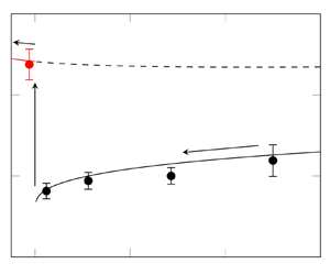
Table 3 and figure 6 show the agreement between experimental values ( $\,f^{\star }_{e}$) and numerical predictions ( $\,f^{\star }_{n}$) of the natural frequency, and confirm the occurrence of the discontinuity at $We=1$. Note that the error bars reported in figure 6 and in last column of table 3 represent the standard deviation ( $s$) of the experimental measurements, whose values vary between $8\,\%$ and $16\,\%$ of the corresponding mean quantities. The reference frequency employed to convert the numerical data ${\rm \Delta} \lambda ^{\pm }_i$ in dimensional form $f^{\star }_{n}$ is $f^{\star }_{ref} = U^{\star }_{in}/ (2 {\rm \pi}L^{\star })$.
Comparison between numerical ( $\,f^{\star }_{n}$, continuous curves) and experimental ( $\,f^{\star }_{e}$, filled circles) natural frequencies in supercritical (black) and subcritical (red) regimes. The numerical frequency associated with the fast branch of the spectrum in supercritical conditions is also reported (black dashed curve). The error bars represent the standard deviation of the experimental measurements.

Experimental and numerical values of the natural frequency varying the Weber number. The relative percentage spread  $\epsilon$ is defined as $\epsilon = 100 \cdot (f^{\star }_{n} - f^{\star }_{e})/f^{\star }_{n}$. The last column reports the standard deviation of the experimental measurements.

5. Conclusions
The free and forced responses of gravitational liquid sheet flows interacting with an unconfined air ambient have been analysed both numerically and experimentally, for various inlet Weber numbers ranging from supercritical ( $We>1$) to subcritical ( $We<1$) conditions. The numerical investigation is based on a linear inviscid one-dimensional model accounting for the coupling between the curtain motion and the ambient pressure disturbances, whose capability of prediction has been already tested by comparison with numerical simulations carried out with a VOF based code. An eigenvalues analysis has been employed to investigate the natural response, while the numerical integration of the governing equations, equipped with an inlet boundary condition including a harmonically oscillating transverse velocity, has provided the forced behaviour of the sheet. Experimental tests have been performed to measure the free response of the flow system by recording the sheet oscillations in its lateral plane with a scanning laser Doppler vibrometer; the flow rate was progressively reduced so as to obtain a transition from the supercritical-to-subcritical regime.
Results of the forced curtain oscillatory dynamics have shown that the sheet response varies continuously when the flow undergoes the supercritical-to-subcritical transition. Considering the analogous result found by Torsey et al. (Reference Torsey, Weinstein, Ross and Barlow2021) in case of an infinite liquid sheet subjected to imposed ambient pressure disturbances not coupled with the curtain motion, and results obtained in the present work neglecting the sheet–ambient interaction (Appendix A), it is inferred that the continuous behaviour of the finite length curtain forced dynamics at the transcritical threshold does not depend on the specific curtain–ambient interaction model considered. On the contrary, the global eigenvalue spectrum obtained by means of the modal analysis clearly shows an abrupt increase in the natural frequency at the transcritical threshold, whose occurrence has been confirmed for the first time by experimental findings.
As a summary, the theoretical prediction of the liquid sheet natural frequency, and therefore its jump when the supercritical-to-subcritical flow transition occurs, strongly relies on two features of the curtain flow model employed here: accounting for the sheet–ambient interaction and considering a sheet of finite length. As a matter of fact, we verified that if one neglects the pressure term in case of a finite length curtain, the linear stability analysis yields an empty spectrum, i.e. no natural frequency is detected, and consequently no frequency discontinuity. On the other hand, if a curtain of infinite length is considered, the natural frequency predicted by the theoretical analysis vanishes.
Acknowledgements
The authors would like to acknowledge L. de Luca for inspiring the work; G. Arena for providing technical assistance using the laser vibrometer; M. Minale and R. Griffo for providing advice and equipment to measure the surface tension, density and viscosity of the working fluid. Finally, the authors would like to acknowledge the anonymous referees for their valuable comments, especially in helping to clarify the separate/combined effects of curtain length and air interactions on natural frequency by recommending the additional analyses reported in the appendices.
Funding
This research received no specific grant from any funding agency, commercial or not-for-profit sectors.
Declaration of interests
The authors report no conflict of interest.
Appendix A. Natural frequency of an infinitely long curtain
The aim of the present section is to show that the liquid sheet natural characteristic frequency, and therefore its jump when the supercritical-to-subcritical flow transition occurs, can only be predicted considering a curtain of finite length  $L^{\star }$ together with the pressure model adopted within this work (§ 4.1). In other words, if a sheet of infinite length is considered, the predicted natural frequency vanishes.
To this purpose, one can introduce the gravitational length scale  $L^{\star }_g = U^{\star 2}_{in}/g$, evaluate the ratio between this scale and the actual curtain length $L^{\star }$, which is also the Froude number, $Fr = U^{\star 2}_{in}/(gL^{\star })$, and consider that an infinitely long curtain corresponds to the condition $U^{\star 2}_{in}/g << L^{\star }$, that is a curtain gravitationally of infinite length. Therefore, in the present analysis the case of infinite length can be investigated as limit case of $Fr\to 0$, which physically corresponds to lengthen progressively the curtain for a given inlet velocity $U^{\star }_{in}$.
For the reasons stated above, the evolution of the liquid sheet natural frequency as the Froude number is progressively reduced, tending to zero, is studied; results are shown in figures 7 and 8, where the eigenvalue spectrum (figure 7a) and the theoretical predictions of the natural characteristic frequency ( ${\rm \Delta} \lambda ^{-}_i$, figures 7(b) and 8(c), and ${\rm \Delta} \lambda ^{+}_i$, figure 8(d), respectively in supercritical and subcritical conditions) are reported. Moreover, the corresponding dimensional values $f^{\star }_n$ are shown in figure 7(c) and figure 8(a,b). The theoretical predictions ${\rm \Delta} \lambda ^{\pm }_i$ are provided, following Girfoglio et al. (Reference Girfoglio, De Rosa, Coppola and de Luca2017), as
 $$\begin{gather} {\rm \Delta} \lambda^{-}_i=\frac{\rm \pi}{Fr\left[\dfrac{1}{2}\left(U|_1-1\right)+ \dfrac{1}{\sqrt{We}}\left(\sqrt{U|_1}-1\right)+ \dfrac{1}{We}\log{\dfrac{\sqrt{U|_1}-\dfrac{1}{\sqrt{We}}}{1-\dfrac{1}{\sqrt{We}}}}\right]} , \end{gather}$$
 $$\begin{gather}{\rm \Delta} \lambda^{+}_i =\dfrac{\rm \pi}{Fr\left[\dfrac{1}{2}\left(U|_1-1\right)-\dfrac{1}{\sqrt{We}}\left(\sqrt{U|_1}-1\right)+ \dfrac{1}{We}\log{\dfrac{\sqrt{U|_1}+\dfrac{1}{\sqrt{We}}}{1+\dfrac{1}{\sqrt{We}}}}\right]}, \end{gather}$$
where  $U|_1 = \sqrt {1 + 2/Fr}$, while the reference quantity employed to convert the data ${\rm \Delta} \lambda ^{\pm }_i$, so as to obtain the (dimensional) natural frequency $f^{\star }_{n}$, is $f^{\star }_{ref} = U^{\star }_{in}/ (2 {\rm \pi}L^{\star })$, as previously done in § 4.2.
Eigenvalue spectrum (a),  ${\rm \Delta} \lambda ^{-}_i$ (b) and curtain natural characteristic frequency $f^{\star }_n$ (c) varying the Froude number. In (b,c), both the theoretical predictions (continuous black curve) and the numerical evaluations from the spectrum (black circles) are reported. Here, $We=1.2$.

Analysis of the curtain natural characteristic frequency  $f^{\star }_n$ in the limit case of $Fr \to 0$ in supercritical (a) and subcritical (b) conditions. The dimensionless values ${\rm \Delta} \lambda ^{\pm }_i$ are also reported (c,d).

By looking at figure 7(c) and figure 8(a,b), it can be appreciated that, as the Froude number decreases, the frequency  $f^{\star }_n$ also decreases, and tends to vanish as $Fr$ approaches zero, both in supercritical and subcritical conditions. Note that, for the supercritical case considered in figure 7 ( $We = 1.2$), two branches of spectrum are obtained, and the natural frequency is associated with the eigenvalues spacing of the upper branch ${\rm \Delta} \lambda ^{-}_i$ (see § 4.1). It is also interesting to note that the dimensionless values ${\rm \Delta} \lambda ^{\pm }_i$ increase as $Fr$ decreases (figures 7(b) and 8(c,d)) as an effect of the adopted length scale $L^{\star }$, which is indeed not appropriate in the current analysis ( $Fr \to 0$) and it has to be replaced by a different one, namely by the gravitational length $L^{\star }_g$, as determined in the study of an infinitely long curtain by Torsey et al. (Reference Torsey, Weinstein, Ross and Barlow2021).
Therefore, we conclude that the theoretical model of unconfined liquid sheet flow adopted in this work predicts a vanishing natural frequency in the limit of  $Fr \to 0$, i.e. for a curtain of infinite length.
Appendix B. Effect of the sheet–ambient interaction on forced curtain shapes
This section aims at showing that, regardless of whether the coupling between the curtain motion and the external ambient is considered in (2.1) and (2.2) via the pressure term (2.5), the forced liquid sheet behaviour analysed in § 4.1 varies continuously in shape and amplitude when traversing the critical threshold  $We=1$. To this purpose, we present in figure 9 results of the curtain oscillatory dynamics obtained both by taking into account the sheet–ambient interaction (continuous curves), i.e. by numerical integration of
 $$\begin{gather} \frac{\partial\ell}{\partial t} + U\frac{\partial\ell}{\partial x} = v, \end{gather}$$
 $$\begin{gather}\frac{\partial v}{\partial t} + U\frac{\partial v}{\partial x} = \frac{1}{We H}\frac{\partial^{2} \ell}{\partial x^{2}} - {\rm \Delta} p_a, \end{gather}$$
which are the same equations as (2.1) and (2.2) (where  ${\rm \Delta} p_a$ is given by (2.5)), and by neglecting it (dotted curves), thus solving
 $$\begin{gather} \frac{\partial\ell}{\partial t} + U\frac{\partial\ell}{\partial x} = v, \end{gather}$$
 $$\begin{gather}\frac{\partial v}{\partial t} + U\frac{\partial v}{\partial x} = \frac{1}{We H}\frac{\partial^{2} \ell}{\partial x^{2}}. \end{gather}$$
Weber number effect on the sheet centreline deflection,  $\ell$, as a function of the streamwise station, $x$, at different fractions of oscillation period $T$:
$T$:  $t=0 T$ (black); $0.25 T$ (red); $0.5 T$ (blue); $0.75 T$ (green). Results of the numerical integration of (B1)–(B2) (continuous curves); (B3)–(B4) (dotted curves). The dashed line denotes the centreline of the unperturbed curtain. From top to bottom: $f^{\star } = 1, 5$ and $20$ Hz.(a) $(We, f^{\star })=(1.05, 1\,\text {Hz})$; (b) $(We, f^{\star })=(0.95, 1\,\text {Hz})$; (c) $(We, f^{\star })=(1.05, 5\,\text {Hz})$; (d) $(We, f^{\star })=(0.95, 5\,\text {Hz})$: (e) $(We, f^{\star })=(1.05, 20\,\text {Hz})$; ( f) $(We, f^{\star })=(0.95, 20\,\text {Hz})$.

The boundary conditions (2.10) and (2.11) introduced in § 4.1 are enforced in both the cases. The numerical investigation is performed in the same flow conditions considered in § 4.1, i.e. for  $We=1.05$ (a,c,e) and $We=0.95$ (b,d, f), and the forcing frequencies considered are $f^{\star }=1, 5$ and $20$ Hz. Note that (B3) and (B4) are the same as those presented by Torsey et al. (Reference Torsey, Weinstein, Ross and Barlow2021) once they are combined and small notational differences rectified.
Two main results arise from the analysis reported in figure 9. First, it can be appreciated that, regardless of whether the coupling between the curtain motion and the ambient pressure disturbances is considered, the sheet response to the imposed sinusoidal velocity perturbation (2.11) varies continuously when the supercritical-to-subcritical transition occurs. Considering the identical result found by Torsey et al. (Reference Torsey, Weinstein, Ross and Barlow2021) in the case of a liquid sheet subjected to imposed ambient pressure disturbances not coupled with the curtain motion, this result further corroborates the considerations reported in § 4.1, namely that the continuous behaviour of forced sheets at the transcritical threshold does not depend on the specific liquid–gas interaction model employed. On the other hand, although the curtain shapes obtained by taking into account or neglecting the curtain–ambient interaction are in qualitatively good agreement, a longer wavelength of the centreline deflection can be detected for the case of no coupling, the effect being more evident at higher forcing frequencies (figure 9e, f).


 Open access

