2.1. Governing equations and UCM model

The governing equations are the incompressible, axisymmetric Navier–Stokes equations in cylindrical coordinates,

(2.1a)$$\begin{gather} \bar{\rho}(\partial_{\bar{t}}\bar{u}+\bar{u}\partial_{\bar{r}}\bar{u}+ \bar{w}\partial_{\bar{z}}\bar{u})={-}\partial_{\bar{r}}\bar{p}+\frac{1}{\bar{r}} \partial_{\bar{r}}(\bar{r}\bar{\sigma}_{{r}{r}})+\partial_{\bar{z}} \bar{\sigma}_{rz}{-\frac{\bar{\sigma}_{{\theta}{\theta}}}{\bar{r}}}, \end{gather}$$

(2.1b)$$\begin{gather}\bar{\rho}(\partial_{\bar{t}}\bar{w}+\bar{u}\partial_{\bar{r}}\bar{w}+\bar{w}\partial_{\bar{z}}\bar{w})={-}\partial_{\bar{z}}\bar{p}+\frac{1}{\bar{r}}\partial_{\bar{r}}(\bar{r}\bar{\sigma}_{rz})+ \partial_{\bar{z}}\bar{\sigma}_{zz}+\bar{\rho} \bar{g}, \end{gather}$$

(2.1c)$$\begin{gather}\frac{1}{\bar{r}}\partial_{\bar{r}}(\bar{r}\bar{u})+\partial_{\bar{z}}\bar{w}=0, \end{gather}$$

where $\bar {\rho }$ is the density of the fluid, $\bar {g}$ is acceleration due to gravity, $\bar {p}$ is pressure, $\bar {t}$ is time, and $\bar {\sigma }$ is the deviatoric stress tensor with components $\bar {\sigma }_{rr}$, $\bar {\sigma }_{rz}$ and $\bar {\sigma }_{zz}$. Overbars denote dimensional quantities and partial derivatives with respect to, e.g. $\bar {r}$, are denoted $\partial _{\bar {r}}$. The coordinates are $(\bar {r},\bar {\theta },\bar {z})$ with associated velocity components $(\bar {u},\bar {v},\bar {w})$; see figure 1. Here, the axial coordinate $\bar {z}$ increases in the downward direction along the tube. The flow is assumed to be axisymmetric, so the $\bar {\theta }$ and $\bar {v}$ components are taken to be zero.

Figure 1.

Sketch of the flow configuration and variable definitions.

A model for the deviatoric stress components is needed to close the system. Many models have been proposed and seen widespread use; here, we choose to use the UCM model. Under the UCM model, each of the stress components $\bar {\sigma }_{ij}$ are assumed to obey the following constitutive equations:

(2.2a) \begin{gather} \bar{\sigma}_{rr}+\bar{\lambda}[\partial_{\bar{t}}\bar{\sigma}_{rr}+ \bar{u}\partial_{\bar{r}}\bar{\sigma}_{rr}+\bar{w}\partial_{\bar{z}} \bar{\sigma}_{rr}-2(\partial_{\bar{r}}\bar{u})\bar{\sigma}_{rr}-2(\partial_{\bar{z}}\bar{u}) \bar{\sigma}_{rz}]=2\bar{\mu} \partial_{\bar{r}}\bar{u}, \end{gather}

(2.2b) \begin{gather} \begin{array}{@{}l@{}} \bar{\sigma}_{rz}+\bar{\lambda}[\partial_{\bar{t}}\bar{\sigma}_{rz}+\bar{u}\partial_{\bar{r}} \bar{\sigma}_{rz}+\bar{w}\partial_{\bar{z}}\bar{\sigma}_{rz}-(\partial_{\bar{r}}\bar{w}) \bar{\sigma}_{rr}-(\partial_{\bar{r}}\bar{u}+\partial_{\bar{z}}\bar{w}) \bar{\sigma}_{rz}-(\partial_{\bar{z}}\bar{u})\bar{\sigma}_{zz}] \\ \quad =\bar{\mu}(\partial_{\bar{z}}\bar{u}+\partial_{\bar{r}}\bar{w}),\end{array} \end{gather}

(2.2c) \begin{gather} \bar{\sigma}_{zz}+\bar{\lambda}[\partial_{\bar{t}}\bar{\sigma}_{zz}+\bar{u}\partial_{\bar{r}} \bar{\sigma}_{zz}+\bar{w}\partial_{\bar{z}}\bar{\sigma}_{zz}-2(\partial_{\bar{r}}\bar{w}) \bar{\sigma}_{rz}-2(\partial_{\bar{z}}\bar{w})\bar{\sigma}_{zz}]=2\bar{\mu}\partial_{\bar{z}}\bar{w}, \end{gather}

(2.2d) \begin{gather} \bar{\sigma}_{\theta\theta}+\bar{\lambda}[\partial_{\bar{t}} \bar{\sigma}_{\theta\theta}+\bar{u}\partial_{\bar{r}}\bar{\sigma}_{\theta\theta}+ \bar{w}\partial_{\bar{z}}\bar{\sigma}_{\theta\theta}]=\displaystyle\frac{2\bar{\mu} \bar{u}}{\bar{r}}, \end{gather}

where $\bar {\lambda }$ is the relaxation time, $\bar {\mu }$ is the dynamic viscosity and where the right-hand side of (2.2) are the components of the rate-of-strain tensor $\bar {\tau }$.

Boundary conditions at the tube wall, $\bar {r}=\bar {a}$, are no-slip,

(2.3)\begin{equation} \bar{u}=\bar{w}=0.\end{equation}

At the free surface, $\bar {r}=\bar {R}(\bar {z},\bar {t})$, the boundary conditions are given by: (i) continuity of tangential stress; (ii) jump in normal stress according to the Young–Laplace equation; and (iii) a kinematic boundary condition,

(2.4a)$$\begin{gather} \bar{\sigma}_{rz}+(\partial_{\bar{z}}\bar{R})(\bar{\sigma}_{rr}-\bar{\sigma}_{zz})- (\partial_{\bar{z}}\bar{R})^2\bar{\sigma}_{rz}=0, \end{gather}$$

(2.4b)$$\begin{gather} \begin{aligned}&-\bar{p}[1+(\partial_{\bar{z}}\bar{R})^2]+\bar{\sigma}_{rr}-2(\partial_{\bar{z}}\bar{R}) \bar{\sigma}_{rz}+(\partial_{\bar{z}}\bar{R})^2\bar{\sigma}_{zz}\\& =\bar{\gamma}[1+(\partial_{\bar{z}}\bar{R})^2]\left(\frac{1}{\bar{R} [1+(\partial_{\bar{z}}\bar{R})^2]^{1/2}}-\frac{\partial_{\bar{z}\bar{z}} \bar{R}}{[1+(\partial_{\bar{z}}\bar{R})^2]^{3/2}}\right),\end{aligned} \end{gather}$$

(2.4c)$$\begin{gather}\bar{u}=\partial_{\bar{t}}\bar{R}+\bar{w}\partial_{\bar{z}}\bar{R}, \end{gather}$$

where the background pressure has been set to zero for convenience.

Equations (2.1)–(2.4) may be non-dimensionalized by the scales

(2.5a{–}g) \begin{align} r=\frac{\bar{r}}{\bar{R}_0},\quad z=\frac{\bar{z}}{\bar{\varLambda}},\quad u=\frac{\bar{u}}{\bar{U}_0},\quad w=\frac{\bar{w}}{\bar{W}_0},\quad t=\frac{\bar{t}\bar{W}_0}{\bar{\varLambda}},\quad p=\frac{\bar{p}}{\bar{\rho} \bar{g}\bar{R}_0},\quad \sigma_{ij}=\frac{\bar{\sigma}_{ij}}{\bar{\rho} \bar{g}\bar{R}_0}, \end{align}

where $\bar {R}_0=\bar {a}-\bar {h}_0$ is the distance from the centre of the tube to the mean free surface of the film, $\bar {\varLambda }$ is a typical wavelength of a free-surface disturbance, and where $\bar {U}_0$ and $\bar {W}_0=\bar {\rho } \bar {g}\bar {R}_0^2/\bar {\mu }$ are velocity scales in the radial and axial directions, respectively. The model development that follows will make use of a long-wave assumption that exploits an assumed small ratio of length scales $\epsilon =\bar {R}_0/\bar {\varLambda }\ll 1$. The continuity equation then dictates that $\bar {U}_0=\epsilon \bar {W}_0$. This results in the following dimensionless governing equations:

(2.6a)$$\begin{gather} \epsilon^2 \widetilde{Re}(\partial_tu+u\partial_ru+w\partial_zu)={-}\partial_rp+ \frac{1}{r}\partial_r(r\sigma_{rr})+\epsilon\partial_z \sigma_{rz}{-\frac{\sigma_{\theta\theta}}{r}}, \end{gather}$$

(2.6b)$$\begin{gather}\epsilon \widetilde{Re}(\partial_tw+u\partial_rw+w\partial_zw)={-}\epsilon \partial_zp+\frac{1}{r}\partial_r(r\sigma_{rz})+\epsilon\partial_z\sigma_{zz}+1, \end{gather}$$

(2.6c)$$\begin{gather}\frac{1}{r}\partial_r(ru)+\partial_zw=0, \end{gather}$$

where $\widetilde {Re}=\bar {\rho } \bar {R}_0\bar {W}_0/\bar {\mu }$ is the Reynolds number. In dimensionless form, the constitutive equations are

(2.7a) \begin{gather} \sigma_{rr}+\epsilon \widetilde{We} [\partial_t\sigma_{rr}+u\partial_r\sigma_{rr}+w\partial_z \sigma_{rr}-2(\partial_ru)\sigma_{rr}-2\epsilon (\partial_zu)\sigma_{rz}]=2\epsilon\partial_ru, \end{gather}

(2.7b) \begin{gather} \begin{array}{@{}l@{}} \sigma_{rz}+ \widetilde{We}[\epsilon\partial_t\sigma_{rz}+\epsilon u\partial_r\sigma_{rz}+ \epsilon w\partial_z\sigma_{rz}-(\partial_rw)\sigma_{rr}-\epsilon(\partial_ru+\partial_zw) \sigma_{rz}-\epsilon^2(\partial_zu)\sigma_{zz}] \\ \quad =\epsilon^2\partial_zu+\partial_rw, \end{array} \end{gather}

(2.7c) $$\begin{gather} \sigma_{zz}+ \widetilde{We}[\epsilon\partial_t\sigma_{zz}+\epsilon u\partial_r\sigma_{zz}+ \epsilon w\partial_z\sigma_{zz}-2(\partial_rw)\sigma_{rz}-2\epsilon (\partial_zw)\sigma_{zz}]=2\epsilon\partial_zw, \end{gather}$$

(2.7d) $$\begin{gather}\sigma_{\theta\theta}+\epsilon \widetilde{We}[\partial_t\sigma_{\theta\theta}+ u\partial_r\sigma_{\theta\theta}+ w\partial_z\sigma_{\theta\theta}]=\frac{2\epsilon u}{r}, \end{gather}$$

where $\widetilde {We}=\bar {\lambda }\bar {W}_0/\bar {R}_0$ is the Weissenberg number, the value of which specifies the ratio of elastic forces to viscous forces in the problem. Boundary conditions at the tube wall, $r=a$, where $a=\bar {a}/\bar {R}_0$, are

(2.8)\begin{equation} u=w=0,\end{equation}

and at the free surface, $r=R(z,t)$,

(2.9a)$$\begin{gather} [1-\epsilon^2(\partial_zR)^2]\sigma_{rz}+\epsilon (\partial_zR)(\sigma_{rr}-\sigma_{zz})=0, \end{gather}$$

(2.9b)$$\begin{gather} -p[1+\epsilon^2(\partial_zR)^2]+\sigma_{rr}-2\epsilon (\partial_zR)\sigma_{rz}+ \epsilon^2(\partial_zR)^2\sigma_{zz}\nonumber\\ =\frac{1}{\widetilde{Bo}}[1+\epsilon^2(\partial_zR)^2] \left(\frac{1}{R[1+\epsilon^2(\partial_zR)^2]^{1/2}}- \frac{\epsilon^2\partial_{zz}R}{[1+\epsilon^2(\partial_zR)^2]^{3/2}}\right),\end{gather}$$

(2.9c)$$\begin{gather} u=\partial_tR+w\partial_zR, \end{gather}$$

where $\widetilde {Bo}=\bar {\rho } \bar {g}\bar {R}_0^2/\bar {\gamma }$ is the Bond number, whose value specifies the ratio of gravity forces to capillary forces. We thus have a total of five dimensionless parameters governing the flow: film thickness parameter $a$, Reynolds number $\widetilde {Re}$, Bond number $\widetilde {Bo}$, Weissenberg number $\widetilde {We}$ and aspect ratio $\epsilon$.

2.2. Leading-order equations and solution

Integrating the continuity equation (2.6c) across the fluid layer and applying the boundary conditions (2.8) and (2.9c) results in an evolution equation for the free surface $R(z,t)$,

(2.10)\begin{equation} \partial_tR=\frac{1}{R}\partial_z\int_R^awr\,{\rm d} r. \end{equation}

All that is needed to close the model is an expression for the axial velocity $w$. To find an approximation of $w$, a regular perturbation expansion in $\epsilon$ is used, with each variable expressed as

(2.11a)$$\begin{gather} w=w_0+\epsilon w_1+O(\epsilon^2),\quad p=p_0+\epsilon p_1+O(\epsilon^2), \end{gather}$$

(2.11b)$$\begin{gather}u=u_0+\epsilon u_1+O(\epsilon^2),\quad \sigma_{ij}=\sigma_{ij,0}+\epsilon \sigma_{ij,1}+O(\epsilon^2). \end{gather}$$

Substituting (2.11) into the governing equations (2.6) and truncating at leading order in $\epsilon$ results in

(2.12a{–}c)\begin{equation} \partial_rp_0=\frac{1}{r}\partial_r(r\sigma_{rr,0}){-\frac{\sigma_{\theta\theta,0}}{r}},\quad \frac{1}{r}\partial_r(r\sigma_{rz,0})={-}1,\quad \frac{1}{r}\partial_r(ru_0)+\partial_zw_0=0, \end{equation}

and the constitutive equations of the UCM model are given by

(2.13a)$$\begin{gather} \sigma_{rr,0}=0, \end{gather}$$

(2.13b)$$\begin{gather}\sigma_{rz,0}-\widetilde{We}(\partial_r w_0)\sigma_{rr,0}=\partial_rw_0, \end{gather}$$

(2.13c)$$\begin{gather}\sigma_{zz,0}-2\widetilde{We}(\partial_r w_0)\sigma_{rz,0}=0, \end{gather}$$

(2.13d)$$\begin{gather}\sigma_{\theta\theta,0}=0. \end{gather}$$

The no-slip boundary condition at $r=a$ dictates $u_0=w_0=0,$ and at $r=R(z,t)$, the boundary conditions are

(2.14) \begin{equation} \sigma_{rz}=0,\quad -p_0+\sigma_{rr,0}=\frac{1}{\widetilde{Bo}}\left(\frac{1}{R}-\epsilon^2R_{zz}\right), \end{equation}

where we have retained one term of higher order in $\epsilon$. While a full discussion of the retention of this term is omitted here, this term is commonly included in long-wave asymptotic models and has been shown to be the first-appearing term in the expansion that prevents shock formation; it also provides the correct cut-off wavenumber for linearly unstable modes and produces excellent agreement with experiments for Newtonian films.

The leading-order solution to (2.12a{–}c)–(2.14) is given by

(2.15) \begin{equation} \left.\begin{gathered} u_0=\frac{R(\partial_zR)}{4r}\left(r^2-a^2-2r^2\log\frac{r}{a}\right),\quad \sigma_{rz,0}=\frac{1}{2r}(R^2-r^2), \\ w_0=\frac{1}{4}\left(a^2-r^2+2R^2\log\frac{r}{a}\right),\quad \sigma_{zz,0}=\frac{\widetilde{We}}{2r^2}(R^2-r^2)^2,\\ p_0={-}\frac{1}{\widetilde{Bo}}\left(\frac{1}{R}-\epsilon^2\partial_{zz}R\right),\quad \sigma_{rr,0}=\sigma_{\theta\theta,0}=0. \end{gathered}\right\} \end{equation}

Note that the presence of elasticity does not modify the leading order base flow $(u,w)$, but does modify the $\sigma _{zz,0}$ component of the stress tensor. Equation (2.15) results in a leading-order model

(2.16)\begin{equation} {\partial_tR=\frac{1}{R}\partial_z\int_R^aw_0r\,{\rm d} r=\frac{1}{2} \left(R^2-a^2-2R^2\log\frac{R}{a}\right)\partial_zR.} \end{equation}

2.3. First-order equations and long-wave model

Next, the base flow may be used to find the first-order axial velocity $w_1$. The case of low-Reynolds-number flow, i.e. $\widetilde {Re}=O(\epsilon )$, is considered first. In this case, the inertial terms appear at $O(\epsilon ^2)$ and the governing equations at first-order in $\epsilon$ are given by

(2.17a)$$\begin{gather} \partial_rp_1=\frac{1}{r}\partial_r(r\sigma_{rr,1})+ \partial_z\sigma_{rz,0}{-\frac{\sigma_{\theta\theta,1}}{r}}, \end{gather}$$

(2.17b)$$\begin{gather}{\frac{1}{r}\partial_r(r\sigma_{rz,1})}=\partial_zp_0-\partial_z\sigma_{zz,0}, \end{gather}$$

(2.17c)$$\begin{gather}\frac{1}{r}\partial_r(ru_1)+\partial_zw_1=0. \end{gather}$$

The UCM model constitutive equations are

(2.18a) \begin{gather} \sigma_{rr,1}=2\partial_ru_0,\end{gather}

(2.18b) \begin{gather}\begin{array}{@{}l@{}} \sigma_{rz,1}+\widetilde{We}[\partial_t\sigma_{rz,0}+u_0 \partial_r\sigma_{rz,0}+w_0\partial_z\sigma_{rz,0} \\ \quad -(\partial_rw_0)\sigma_{rr,1}-(\partial_rw_1) \sigma_{rr,0}-(\partial_ru_0+\partial_zw_0)\sigma_{rz,0}]=\partial_rw_1, \end{array} \end{gather}

(2.18c) \begin{gather} \begin{array}{@{}l@{}} \sigma_{zz,1}+\widetilde{We}[\partial_t\sigma_{zz,0}+u_0\partial_r \sigma_{zz,0}+w_0\partial_z\sigma_{zz,0}\\ \quad -2(\partial_rw_0)\sigma_{rz,1}-2(\partial_rw_1) \sigma_{rz,0}-2(\partial_zw_0)\sigma_{zz,0}]=2\partial_zw_0,\end{array} \end{gather}

(2.18d) \begin{gather} \sigma_{\theta\theta,1}=\frac{2u_0}{r}. \end{gather}

Once again, no-slip boundary conditions apply at the wall $r=a$, while at the free surface $r=R(z,t)$, the first-order boundary conditions are

(2.19a)$$\begin{gather} \sigma_{rz,1}+(\partial_zR)(\sigma_{rr,0}-\sigma_{zz,0})=0, \end{gather}$$

(2.19b)$$\begin{gather}-p_1+\sigma_{rr,1}-2(\partial_zR)\sigma_{rz,0}=0. \end{gather}$$

While each equation and condition has been given through first-order, only (2.17b), (2.18a), (2.18b) and (2.19a) are needed to derive the first-order axial velocity $w_1$. In solving for $w_1$, note that (2.18b) contains $\partial _t\sigma _{rz,0}=RR_t/r$; to evaluate this contribution from the leading order stress, we use the leading order model (2.16) to substitute for $\partial _tR$. This approach is identical to that taken by e.g. Camassa et al. (Reference Camassa, Ogrosky and Olander2014) to incorporate inertial effects. Note that this approach may not be applicable to settings without a base flow, as considered by Halpern et al. (Reference Halpern, Fujioka and Grotberg2010), for example. This results in the following expression for $w_1$:

(2.20)\begin{align} {w_1}&=\frac{1}{4\widetilde{Bo}}\left(r^2-a^2-2R^2\log\frac{r}{a}\right) \left(\frac{\partial_zR}{R^2}+\partial_{zzz}R\right) \nonumber\\ &\quad +\frac{\widetilde{We}R(\partial_zR)}{8} \left[r^2-a^2-R^2+\frac{a^2R^2}{r^2}+2(a^2-R^2)\log\frac{r}{a} \vphantom{\left(\log\frac{R}{a}+\log\frac{R}{r}\right)}\right. \nonumber\\ &\quad \left. +\;4R^2\log\frac{r}{a}\left(\log\frac{R}{a}+\log\frac{R}{r}\right)\right]. \end{align}

Using (2.15) and substituting $w_0+\epsilon w_1$ into (2.10), the model equation is

(2.21)\begin{equation} \partial_tR=\frac{1}{16R}{\partial_z}\left[f_1(R;a)\left(1-\frac{a^2}{Bo} \left(\frac{\partial_zR}{R^2}+\partial_{zzz}R\right)\right)-\frac{{We}R(\partial_zR)}{2a}f_2(R;a)\right], \end{equation}

where

(2.22a)$$\begin{gather} f_1(R;a)=a^4-4a^2R^2+3R^4-4R^4\log\frac{R}{a}, \end{gather}$$

(2.22b)$$\begin{gather}f_2(R;a)=3a^4-3R^4-4R^4\log\frac{R}{a}+16a^2R^2\log\frac{R}{a}+8R^4\left(\log\frac{R}{a}\right)^2, \end{gather}$$

and where we have dropped the $\epsilon$'s from the final model equation. This corresponds to returning to the original aspect ratio in the dimensionless problem; while the $\epsilon$'s are no longer in the model equation, it must be pointed out that the strict validity of the model derivation still relies on the assumption $\epsilon \ll 1$ is satisfied. Note that (2.21) has been expressed in terms of a rescaled Bond number ${Bo}=a^2\widetilde {Bo}$ and Weissenberg number ${We}=a\widetilde {We}$; these rescaled numbers ${Bo}=\bar {\rho }\bar {g}\bar {a}^2/\bar {\gamma }$ and ${We}=\bar {\lambda }\bar {\rho }\bar {g}\bar {a}/\bar {\mu }$ have the advantage of being independent of film thickness and depend only on parameters density, viscosity, tube radius, surface tension and relaxation time. It is interesting to note that the same model equation may be derived using the Oldroyd-B constitutive equations in place of the UCM model, so that the dynamical outcomes produced by either constitutive model are identical. Note that $f_i(R;a)>0$ (for $i=1,2$) since $0< R< a$.

In the case where ${Re}=O(1)$, the inertial terms appear at first-order; the details of the derivation in the case of a Newtonian film can be found from Camassa et al. (Reference Camassa, Ogrosky and Olander2014) and are omitted here as the resulting terms are identical (up to choice of scales):

(2.23)\begin{align} \partial_tR &= \frac{1}{16R}{\partial_z}\left[f_1(R;a)\left(1-\frac{a^2}{Bo} \left(\frac{\partial_zR}{R^2}+\partial_{zzz}R\right)\right) \right.\nonumber\\ &\quad \left.-\frac{{We}R(\partial_zR)}{2a}f_2(R;a)-\frac{Re}{a^3}f_3(R;a)\partial_zR\right], \end{align}

where

(2.24)\begin{align} f_3(R;a)&=\tfrac{59}{48}R^7-\tfrac{15}{16}a^2R^5-\tfrac{9}{16}a^4R^3+\tfrac{13}{48}a^6R- \tfrac{17}{4}a^2R^5\log (R/a)+\tfrac{7}{4}a^4R^3\log (R/a) \nonumber\\ &\quad -\tfrac{5}{2}R^7(\log(R/a))^2+\tfrac{5}{2}a^2R^5(\log (R/a))^2+2R^7(\log(R/a))^3, \end{align}

and where ${Re}=a^3\widetilde {Re}=\bar {\rho }^2\bar {g}\bar {a}^3/\bar {\mu }^2$ is a rescaled Reynolds number. As the focus here is on highly viscous films, model results will be primarily presented for (2.21), but comments will be given on (2.23) as well. It is again the case that $f_3(R;a)>0$ for $0< R< a$.

In the thin-film limit, the nonlinearities in the model simplify considerably. A film thickness $h$, scaled so that $h=0$ at the wall and $h=1$ at the mean free surface, may be defined by

(2.25)\begin{equation} h=\frac{a-R}{a-1}. \end{equation}

Substituting $R=a-\beta h$, with $\beta =a-1$, into (2.21) and expanding about $\beta =0$ results in

(2.26)\begin{equation} \partial_th+\frac{1}{3}{\partial_z}\left[h^3\left(1+\frac{1}{Bo^*}(\partial_zh+\partial_{zzz}h)\right)+ {We}^* h^4(\partial_zh)\right]=0, \end{equation}

where ${Bo}^*={Bo}/\beta$, ${We}^*=\beta ^2{We}$ and where time has been rescaled by $\beta ^2$. Equation (2.26) is similar to that of Frenkel (Reference Frenkel1992) but with viscoelasticity included, and is also similar to that of Kang & Chen (Reference Kang and Chen1995) for flow down an inclined plane but includes the effects of azimuthal curvature. Note that the viscoelastic term is proportional to $h^4$, while surface tension and advection terms contain $h^3$. In that respect – having a higher-order term that will be shown to drive instability growth – it bears some resemblance to the equation derived by Benney (Reference Benney1966) for film flow down an inclined plane, in which instability growth is provided by an inertial term proportional to $h^6$. For certain parameter values, unbounded solutions to this Benney equation can arise, which has no physical relevance for the falling-film-down-plane problem; this issue can be addressed through use of the WRIBL modelling approach (see, e.g. Ruyer-Quil & Manneville Reference Ruyer-Quil and Manneville1998; Dietze & Ruyer-Quil Reference Dietze and Ruyer-Quil2015). It would be interesting to conduct a detailed study of (2.26) for similar features, especially since unbounded solutions are not necessarily physically irrelevant given the potential for plug formation in the tube problem considered here, but nonlinear results will be presented here strictly for the model (2.21).

2.4. Parameter values

Before presenting model results, a brief discussion is given concerning the range of parameter values for Bo, ${Re}$, We and $a$ that are in mind here. As the model is derived to consider highly viscous flows, we briefly consider some experimental set-ups for which this model could apply.

In the Newtonian experiments of Camassa et al. (Reference Camassa, Ogrosky and Olander2014), a highly viscous silicone oil is used as the solvent, with density, dynamic viscosity and surface tension given approximately by

(2.27a{–}c)\begin{equation} \bar{\rho}=0.97\,\textrm{g}\,\textrm{cm}^{{-}3},\quad \bar{\mu}=125\,\textrm{P},\quad \bar{\sigma}=21.5\,\textrm{dyn}\,\textrm{cm}^{{-}1}, \end{equation}

respectively. The inner radius $\bar {a}$ of the tube in the experiments ranged from 0.5 cm down to $0.17$ cm; the thickness of the film $\bar {h}_0$ in viscous gravity-driven experiments varied, but most experiments had film thicknesses between 0.1 and 0.2 cm. Using these values results in the following estimated ranges for the dimensionless parameters in the model for a Newtonian fluid,

(2.28a{–}c) \begin{equation} {Bo}=1.3-11.1,\quad {Re}=3\times10^{{-}4}-7\times10^{{-}3},\quad a=1.25-2.5. \end{equation}

As ${Re}<0.01$ for all these cases, the focus will primarily be on the inertialess model (2.21), with values of Bond number primarily lying in the range $0.5<{Bo}<15$ and tube radius parameter $1< a<3$, occasionally showing results for other values of Bo or $a$ to illustrate a point about the model.

For viscoelastic films, Shaqfeh, Larson & Frederickson (Reference Shaqfeh, Larson and Frederickson1989) (see also Kang & Chen Reference Kang and Chen1995) found that the Oldroyd-B model is capable of capturing the behaviour of polymeric thin films so long as ${We}<2.5$. Based on this criteria, and given that the model equation here is identical to that obtained using the Oldroyd-B equations, we will largely restrict results to ${We}<2.5$.

The addition of polymers to a Newtonian fluid may also modify the surface tension; e.g. an increase in ${We}$ may in some cases be accompanied by a corresponding increase in Bo. This effect was seen, e.g. in experiments conducted by Olander (Reference Olander2020), in which the falling film consisted of polybutene (PB) and various small concentrations of polyisobutylene (PIB); the PIB concentrations were small enough to result in negligible values of ${We}$ but still lower the value of $Bo$ through reduction of the surface tension. Some attention will thus be given to the increase in Bo required to offset a given increase in ${We}$ to produce an equivalent dynamical outcome.

One of the motivations for the experimental values chosen by Camassa et al. (Reference Camassa, Ogrosky and Olander2014) was the study of mucus lining human airways; the viscosities, surface tension and tube radii (and hence ${Bo}$) were chosen to be representative of upper airways. The rheological properties of human mucus can vary widely with patient, disease and airway generation, with elasticity decreasing with airway generation and increasing in the presence of airway diseases like cystic fibrosis (Lai et al. Reference Lai, Wang, Wirtz and Hanes2009).

3.1. Temporal linear stability analysis

To study the linear stability of a flat-interface solution $R(z,t)=1$, let the free surface be perturbed by a superposition of small-amplitude Fourier modes,

(3.1)\begin{equation} R=1+\hat{R}\exp({{\rm i}(kz-\omega t)}),\end{equation}

where $k$ is a spatial wavenumber and where it is assumed that $\hat {R}\ll 1$; while exploring the temporal stability of the free surface, the wavenumber $k$ will be taken to be real-valued. Substituting (3.1) into (2.21) results in the dispersion relation

(3.2)\begin{equation} \omega=\frac{k}{2}(a^2-1-2\log a)+\frac{{\rm i}a^2}{16{Bo}}({k^2}-k^4)f_1(1;a)+ \frac{{\rm i}{We}\,k^2}{32a}f_2(1;a). \end{equation}

The real part of (3.2), $\textrm {Re}[\omega ]/k$, determines the phase speed of disturbances, while the imaginary part, $\textrm {Im}[\omega ]$, dictates the growth of their amplitude. As with other thin-film models, the dispersion relation is similar to that of the Kuramoto–Sivashinsky (KS) equation in the dependence on wavenumber $k$. For reference, the dispersion relation for the model with inertial terms (2.23) and for the inertialess thin-film model (2.26) are also included:

(3.3) \begin{align} \omega=\frac{k}{2}(a^2-1-2\log a)+\frac{{\rm i}a^2}{16{Bo}}({k^2}-k^4)f_1(1;a)+ \frac{{\rm i}{We}\,k^2}{32a}f_2(1;a)+\frac{{\rm i}{Re} k^2}{16a^3}f_3(1;a) \end{align}

and

(3.4)\begin{equation} \omega=\frac{1}{3}\left(k+\frac{{\rm i}\beta }{Bo}(k^2-k^4)+{\rm i}{We}\beta^2k^2\right), \end{equation}

respectively.

Equation (3.2) has been well studied for Newtonian films (${We}=0$); similar to other settings where the Plateau–Rayleigh instability is the dominant one, the film is unstable to long-wave disturbances with cut-off wavenumber $k_c=1$ and the wavenumber of maximum growth rate, $k_{max}=1/\sqrt {2}$, set by a balance of destabilization of the free surface due to its azimuthal curvature and stabilization due to its axial curvature, both arising due to surface tension. The phase speed of disturbances is set by the balance of gravity and viscous forces. In the linear regime, the dimensionless growth rates of this model are determined by the $k^2$ and $k^4$ terms arising due to the Plateau–Rayleigh instability, with the growth rates increasing monotonically with $a$ and with $1/{Bo}$. The inclusion of base flow due to gravity in this first-order model does not impact these dimensionless growth rates as the hyperbolic terms in (2.21) associated with the effects of gravity arise solely in the real part of the dispersion relation, similar to many other first-order film flow models with base flow. This model dispersion relation has been shown to agree well with that of the Stokes equations (Camassa et al. Reference Camassa, Ogrosky and Olander2014).

In the case where ${We}>0$, the presence of elasticity introduces a second mechanism of free-surface destabilization. Figure 2(a) shows the growth rates $\textrm {Im}[\omega (k)]$ (3.2) for $a=1.4$, ${Bo}=1$ and a variety of ${We}$ values; the growth rate increases with increasing ${We}$ for all wavenumbers $k$. The $k^2$ terms of (3.2) are identical to those of Zhou et al. (Reference Zhou, Peng, Zhang and Zhuge2014) in their long-wave analysis without surfactant. Both the wavenumber $k_{max}$ of maximum growth rate and the cutoff wavenumber $k_c$ increase as well, according to

(3.5a,b) \begin{equation} k_c=\sqrt{1+\frac{{We}\,{Bo}\, f_2(1;a)}{2a^3f_1(1;a)}},\quad k_{max}=k_c/\sqrt{2}, \end{equation}

so that the product ${Bo}\,{We}=\bar {\lambda }\bar {\rho }^2\bar {g}^2\bar {a}^3/\bar {\mu }\bar {\gamma }$ determines the change in $k_{max}$ and $k_c$ for fixed $a$. Figure 2(b) shows this dependence of $k_c$ and $k_{max}$ on ${We}$ for $a=1.4$. As the value of Bo increases, changing ${We}$ results in a larger change in $k_{max}$.

Figure 2.

(a) Growth rates of (2.21) for $a=1.4$, ${Bo}=2$ and various values of We. Here, $\times$ symbols denote the maximum growth rate $GR_{max}$ and ${\cdot }$ symbols denote cutoff wavenumber $k_c$. (b) $k_{max}$ and $k_c$ for $a=1.4$ and various values of Bo and We. (c) Same as panel (a) but with $a=1.05$. (d) $f_2(1;a)/[a^3f_1(1;a)]$; maximum value obtained at $a\approx 1.375$. Open circles denote $a$ values used in panels (a,c).

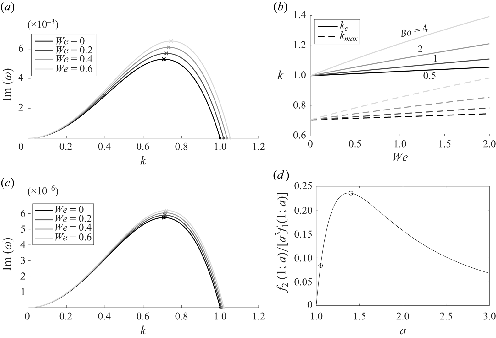
As with the Newtonian film, the growth rates increase with $a$ and $1/{Bo}$, but the relative impact of increasing ${We}$ depends non-monotonically on film thickness parameter $a$. Figure 2(c) shows the growth rates for a much thinner film with $a=1.05$. As may be expected, the growth rates are smaller than for $a=1.4$, but it is also true that the growth rate curves are closer together than in figure 2(a), indicating that increasing ${We}$ has a smaller relative impact on the growth rates and on $k_{max}$ when $a=1.05$ than when $a=1.4$. This may be anticipated from (3.5a,b) or from the thin-film dispersion relation (3.4) in which the term proportional to ${We}$ occurs at higher order in $\beta$ than the other terms.

For moderate values of $a$, the impact of $a$ on $k_{max}$ must be assessed by examining $f_2(1;a)/[a^3f(1;a)]$ in (3.5a,b); this quantity is plotted in figure 2(d). This value reaches a maximum at $a\approx 1.375$; i.e. this value of $a$ produces the largest impact on $k_{max}$ and largest relative impact on the maximum growth rate $GR_{max}$ for small ${We}$ as determined by $[(\partial GR_{max}/\partial We)/GR_{max}]|_{We=0}=f_2(1;a)Bo/[a^3f_1(1;a)]$. We also note that for thick films (large $a$), the relative impact of viscoelasticity on $k_{max}$ and growth rates is again small, as $f_2(1;a)/[a^3f_1(1;a)]$ behaves like $1/a^3$ for large $a$.

In summary, linear instability is driven by both surface tension and viscoelasticity. While growth rates increase monotonically with $a$ and $1/{Bo}$, the relative impact of viscoelasticity on growth rates is highest for moderately thick films.

Note that while the base flow $w_0$ is unchanged by the presence of viscoelasticity, the normal stress is positive, $\sigma _{zz,0}>0$. This stress term plays a crucial role in determining the sign of the first-order velocity $w_1$ through (2.17b); $w_1$ may be expressed as the sum of three parts:

(3.6)\begin{equation} {w_1=w_{ST}+w_{NS}+w_{UCM},} \end{equation}

where

(3.7a) $$\begin{gather} {w_{1,ST}}=\frac{1}{4\widetilde{Bo}}\left(r^2-a^2-2R^2\log\frac{r}{a}\right) \left(\frac{\partial_zR}{R^2}+\partial_{zzz}R\right), \end{gather}$$

(3.7b) $$\begin{gather}{w_{1,NS}}=\frac{\widetilde{We}RR_z}{2}\left(r^2-a^2+2R^2\log\frac{a}{r} \left(1+\log\frac{a}{R}+\log\frac{r}{R}\right)\right), \end{gather}$$

(3.7c) \begin{gather}\begin{array}[b]{@{}l@{}} \displaystyle{w_{1,UCM}}=\frac{\widetilde{We}RR_z}{8}\left(3a^2-3r^2-R^2+\frac{a^2R^2}{r^2}+6R^2 \log\frac{r}{a} \right.\\ \displaystyle\phantom{{w_{1,UCM}}=}\left.+\;2a^2\log\frac{r}{a}-4R^2\log\frac{r}{a}\left(\log\frac{R}{a}+\log\frac{R}{r}\right)\right), \end{array} \end{gather}

where ST denotes surface tension, NS denotes normal stress corresponding to $\sigma _{zz,0}$ and UCM refers to the contribution of the terms in brackets in (2.18b). For $R< r< a$, note that if $R_z>0$, then $w_{1,NS}<0$, $w_{1,UCM}>0$ and $w_{1,NS}+w_{1,UCM}<0$. As a result, the normal stresses (specifically the gradient $\partial _z\sigma _{zz,0}$) generated by the base flow are responsible for the instability growth seen in the current model.

3.2. Absolute and convective instability

Linear stability analysis may also be conducted from a spatio-temporal viewpoint, which allows classification of instabilities as absolute or convective. In experiments, convectively unstable films are those in which visible instability growth is only evident downstream, far from the inlet, while absolutely unstable films exhibit visible instability growth right at or near the inlet.

Deissler, Oron & Lee (Reference Deissler, Oron and Lee1991) first classified instabilities for a falling Newtonian film on the exterior of a tube by applying the methods developed and explored by Bers (Reference Bers1983), Briggs (Reference Briggs1964) and Huerre & Monkewitz (Reference Huerre and Monkewitz1990) among others. They identified a critical velocity separating absolute instability from convective instability for a two-dimensional KS equation, with the critical velocity dependent on the azimuthal mode number. Duprat et al. (Reference Duprat, Ruyer-Quil, Kalliadasis and Giorgiutti-Dauphine2007) applied these techniques to a strongly nonlinear model similar to (2.21) with ${We}=0$ for the exterior case. First finding a critical value for the thin-film parameter ${Bo}^*$ and then transforming the thin-film dispersion relation to the long-wave dispersion relation through a substitution, Duprat et al. (Reference Duprat, Ruyer-Quil, Kalliadasis and Giorgiutti-Dauphine2007) identified a condition on Bond number ${Bo}^*$ and film thickness parameter $a$ that must be met for films to be absolutely unstable. Camassa et al. (Reference Camassa, Ogrosky and Olander2014) later applied this approach to identify a threshold thickness for Newtonian films inside a tube; films thicker than this threshold were shown to be absolutely unstable, while thinner films were convectively unstable.

We briefly state this threshold condition for the Newtonian case. The dispersion relation of the Newtonian case (denoted by subscripts of $N$),

(3.8)\begin{equation} \omega_N=\frac{k_N}{2}(a^2-1-2\log a)+\frac{{\rm i}a^2}{16{{Bo}_N}}({k_N^2}-k_N^4)f_1(1;a), \end{equation}

exhibits absolute instability if the criteria

(3.9)\begin{equation} {\frac{2a^2f_1(1;a)}{{Bo}_N(a^2-1-2\log a)}>8({-}17+7\sqrt{7})^{1/2}} \end{equation}

is met, where ${Bo}_N$ denotes the Bond number in the Newtonian case. This condition matches that found by Camassa et al. (Reference Camassa, Ogrosky and Olander2014) (adjusted for choice of scalings), and arises from considering branches of solutions to (3.8) found for complex wavenumber $k$ and identifying parameter values at which distinct branches coalesce (see, e.g. Huerre & Monkewitz (Reference Huerre and Monkewitz1990), Duprat et al. (Reference Duprat, Ruyer-Quil, Kalliadasis and Giorgiutti-Dauphine2007) and Camassa et al. (Reference Camassa, Ogrosky and Olander2014) for further discussion and a thorough derivation of this criteria).

How does the presence of elasticity affect this condition? The dispersion relation of the Newtonian case (3.8) may be transformed into (3.1) through the substitution

(3.10a,b) \begin{align} {(k_N,\omega_N)=\left(1+\frac{{We}\, {Bo} f_2(1;a)}{2a^3f_1(1;a)}\right)^{{-}1/2}(k,\omega),\quad {Bo}_N=\left(1+\frac{{We}\, {Bo} f_2(1;a)}{2a^3f_1(1;a)}\right)^{{-}3/2}{Bo}.} \end{align}

Substituting (3.10a,b) into (3.9) results in the following condition for absolute instability:

(3.11)\begin{equation} \frac{2{Bo}^{1/2}f_1(1;a)}{a(a^2-1-2\log a)}\left(\frac{a^2}{Bo}+ \frac{{We} f_2(1;a)}{2af_1(1;a)}\right)^{3/2}>8({-}17+7\sqrt{7})^{1/2}. \end{equation}

Figure 3 shows the $a$-Bo boundary between absolute and convective instability for a variety of ${We}$ values. For ${We}=0$, the boundary between absolute and convective instability monotonically increases with increasing Bo. For large values of Bo (or $a$), the boundary is governed by ${Bo}\approx a^4/[4(-17+7\sqrt {7})^{1/2}]$, which may be found by using $f_1(1;a)=a^4+O(a^2)$ and $f_2(1;a)=3a^4+O(a^2)$ in (3.11).

Figure 3.

(a) Boundary in Bo-$a$ space between absolute and convective instability for a variety of ${We}$ values. (b) Same as panel (a) but for a larger range of Bo values. Blue dots denote maximum values of $a$ obtained along each curve.

Increasing ${We}$ results in a greater region of absolute instability, with the effect most pronounced for larger Bo values. In contrast to the ${We}=0$ case, the boundary for ${We}>0$ exhibits non-monotonic behaviour, reaching some maximum attainable value of $a_c$ for a given fixed positive ${We}$. This maximum value, denoted by blue dots in figure 3(b), occurs when ${Bo}=4a^3f_1(1;a)/[{We} f_2(1;a)]$. Past this value of Bo, the boundary decreases monotonically as ${Bo}\rightarrow \infty$, the scaling of which may be found in the thin-film limit by substituting $a=1+\beta$ and $Bo=b\beta ^{\alpha }$ into (3.11) with $\beta \ll 1$. This results in

(3.12)\begin{equation} \frac{16\beta^{1-\alpha}}{3b}(1+{We} b \beta^{\alpha+1})^{3/2}>8({-}17+7\sqrt{7})^{1/2}. \end{equation}

There are two consistent scalings possible, corresponding to one of the two terms inside parentheses providing the dominant balance with the right-hand side of (3.12). If the second term dominates, then $\alpha =-5$ and ${Bo}={9(-17+7\sqrt {7})}/{4{We}^3\beta ^5}$, corresponding to the border between absolute and convective instability for large Bo. The other scaling, with $\alpha =1$ and ${Bo}=2\beta /[3(-17+7\sqrt {7})^{1/2}]$, corresponds to the border for small Bo and is independent of ${We}$.

4.1. Evolution equation

A finite difference method was used to solve (2.21) numerically. Spatial derivatives were calculated using fourth-order approximations; time-stepping was done with an explicit second-order predictor-corrector method. An initial condition was prescribed by perturbing a constant free surface with a superposition of small-amplitude Fourier modes. In a typical simulation, 40 modes were used to perturb the free surface, though a variety of values were tried. The number of initial modes played a role in the transient dynamics as instabilities initially grew, but once the evolution had settled into a quasi-steady state, there was – in almost all cases – no clear signature of the initial conditions. The one exception to this is for films with a mean thickness very near the critical thickness – in which plug formation would only be triggered by wave mergers and not linear wave growth – where a change in initial conditions could result in a change of the final state (plug or no plug) in the finite-time simulations conducted. This was also noted in a study of Newtonian films with wall slip; see Schwitzerlett et al. (Reference Schwitzerlett, Ogrosky and Topaloglu2023) for numerical tests and further discussion of this point.

At $z=0$, inlet boundary conditions were prescribed by populating several ghost nodes upstream of the inlet using a periodic extension of the initial condition moving at the linear phase speed of the free-surface disturbances. At $z=L$, outlet boundary conditions were prescribed by populating several ghost nodes downstream of the inlet using a reflection of the final nodes within the domain. Other outlet boundary conditions were also tried; the exact prescription of these ghost nodes downstream only had a significant impact on the final few nodes near $z=L$, which will be largely ignored in the results. Simulations were also conducted using periodic boundary conditions. Since the dynamical outcomes of the simulations did not change when the boundary conditions were varied, these results are omitted, and results using inlet/outlet boundary conditions will be presented here.

Two dynamical outcomes are evident in simulation snapshots shown in figure 4(a–c). The baseline case in figure 4(a) shows a snapshot of the film in the tube using ${Bo}=10$, ${We}=0$ and $a=1.8$. This snapshot is taken near $t=500$, long after the dynamics have settled into a quasi-steady state. The gently perturbed film entering the domain at the inlet (left) is clearly convectively unstable, with disturbances growing as the film falls down the tube. Between $z=100$ and $z=150$, this growth saturates, with the remainder of the tube coated with a wavy film consisting of small-amplitude travelling-wave-like ripples.

Figure 4.

(a–c) Snapshots of the film evolution for $a=1.8$ and for various Bo and We values. In panels (b,c), the snapshot is taken just prior to the formation of the first plug. (d) Maximum and minimum values of $R$ over the domain in each simulation as a function of $t$.

A second outcome is shown in figure 4(b) with identical parameter values to figure 4)(a) except for ${Bo}=5$. The film is still convectively unstable, but visible growth is seen closer to the inlet, e.g. near $z\approx 50$; the free-surface waves also have larger amplitude than with ${Bo}=10$. However, the simulation is halted near $t=150$ as one of the waves – near $z=220$ – begins to undergo accelerated growth, with the free surface at the wave crest approaching $R=0$ in finite time. Figure 4(d) shows the evolution of $\max R$ and $\min R$ over the domain as a function of time. As with other studies of asymptotic models, $R$ approaching zero may be taken as the model's prediction that plug formation is about to occur. No attempt is made here to continue running the model forward past this time, as the nonlinearities in (2.21) include logarithms and inverse powers of $R$, preventing the model from being run forward as it is, though there has been interesting recent work in this direction. Most notably, Dietze et al. (Reference Dietze, Lavalle and Ruyer-Quil2020) modified a WRIBL model for film flow inside a tube to prevent $R$ from reaching a value of zero during plug formation; this was achieved through inclusion of a novel pressure term that allowed for arbitrarily narrow filaments of core fluid (air) to form where the model exhibited plug formation. Here, the focus is on whether plugs may be expected to form or not, and their propagation after formation is left for future work.

Figure 4(a,b) indicates that for $a=1.8$, there is some critical Bond number $5< {Bo}_c<10$ such that for ${Bo}>{Bo}_c$, plugs do not form; while for ${Bo}<{Bo}_c$, plugs do form. This is consistent with previous work (Camassa et al. Reference Camassa, Ogrosky and Olander2014; Dietze et al. Reference Dietze, Lavalle and Ruyer-Quil2020; Ogrosky Reference Ogrosky2021) showing that stronger base flow inhibits plug formation in Newtonian films. The impact of viscoelasticity is examined next.

Figure 4(c) shows a snapshot of the film with ${Bo}=10$, ${We}=0.9$ and $a=1.8$; note that all three panels of figure 4 have the same value of film thickness parameter $a$. Once again, the film is convectively unstable, though instability growth is visible even closer to the inlet, consistent with the higher linear growth rates found in § 3. The free-surface waves with $We>0$ appear to have shorter typical wavelength than those with $We=0$; e.g. in the simulation snapshots shown in figure 4, the average wavelength from $z=100$ to $z=300$ was approximately 9.5 in figure 4(b) and 7.7 in figure 4(c). This shorter average wavelength may be expected given the impact of viscoelasticity on wavelength shown in (3.5a,b). Similar to figure 4(b), the simulation was halted (near $t=95$) as one wave – near $z=150$ – underwent accelerated amplitude growth, resulting in $R\rightarrow 0$ indicating plug formation.

The results above indicate that either increasing ${We}$ or decreasing Bo past some critical value while holding the film thickness constant results in plug formation. Said another way, for fixed Bo and ${We}$, there is a critical value of $a$ such that if $a$ exceeds this value, plug formation may be expected to occur; increasing ${We}$ or decreasing Bo leads to a reduction in this critical value of $a$.

4.2. Travelling wave solutions

Since the free surface in figure 4 evolves into a travelling wave train, travelling wave solutions are sought next. Substituting $Q(Z)=Q(z-ct)=R(z,t)$ into (2.21) and integrating once results in a third-order ordinary differential equation,

(4.1)\begin{equation} 8cQ^2+K+\left[1-\frac{a^2}{Bo}\left(\frac{Q'}{Q^2}+Q'''\right)\right]f_1(Q;a)-\frac{{We}\,QQ'}{2a}f_2(Q;a)=0, \end{equation}

with speed $c$ and constant of integration $K$. The approach used to find solutions to this ODE follows the approach outlined by Camassa et al. (Reference Camassa, Marzuola, Ogrosky and Vaughn2016) and is briefly outlined here. First, fixed point solutions are found for the three-dimensional dynamical system associated with (4.1); these correspond to constant solutions $Q=Q_0$. If the wave speed $c$ is varied, a Hopf bifurcation in the solution family is identified using XPP/AUTO; XPP is a numerical tool for simulating and analysing dynamical systems (Ermentrout Reference Ermentrout2002) and also provides a front end to the numerical continuation and bifurcation package AUTO (Doedel et al. Reference Doedel, Champneys, Dercole, Fairgrieve, Kuznetsov, Oldeman, Paffenroth, Sandstede, Wang and Zhang2008). This bifurcation is a zero-Hopf bifurcation, which can be somewhat difficult to find numerically; to avoid this issue, a small viscosity-like term $\eta Q''$ was added to (4.1) which makes continuation onto a family of periodic solutions easier. Once periodic solutions have been found, the viscosity parameter $\eta$ may be taken to zero. The mean value of $Q^2$ is ensured to be equal to one by imposing an integral condition. As the focus here is on waves with profiles similar to those seen in transient solutions like figure 4, only solution families with such profiles are presented here; other families, e.g. were considered by Zhou et al. (Reference Zhou, Peng, Zhang and Zhuge2016) for an integral boundary layer model.

Figure 5(a) shows several families of travelling wave solutions with period $4{\rm \pi}$ for a variety of values of Bo and ${We}$; the period $4{\rm \pi}$ was chosen as it is approximately the period of waves for ${We}=0$ seen in figure 4(a) especially near the bottom of the tube, e.g. from $z=150$ to $z=250$. Each curve shows the wave amplitude of solutions within a family as a function of film thickness parameter. Before discussing the impact of viscoelasticity on these curves, we first note that each family has a turning point (denoted by a red dot) at some critical value $a_c$ of the thickness parameter $a$. For ${We}=0$, this critical thickness $a_c$ has previously been shown to be a reliable proxy for the critical thickness required for plugs to form (Camassa et al. Reference Camassa, Ogrosky and Olander2014, Reference Camassa, Marzuola, Ogrosky and Vaughn2016; Ding et al. Reference Ding, Liu, Liu and Yang2019; Dietze et al. Reference Dietze, Lavalle and Ruyer-Quil2020; Camassa et al. Reference Camassa, Marzuola, Ogrosky and Swygert2021). The critical thickness associated with the turning point solution depends on the value of Bo, with higher values of Bo corresponding to higher critical thickness, consistent with the results of § 4.1 and with the results of Dietze et al. (Reference Dietze, Lavalle and Ruyer-Quil2020) showing that while the base flow does not contribute to the linear growth/decay of small disturbances, it plays a nonlinearly stabilizing role. Note that the horizontal axis shows $(a-1)/a$, with values close to 0 representing thin films, and values close to 1 representing thick films (since in the limit $a\rightarrow 1$ (thin films), $(a-1)/a\rightarrow 0$, while in the limit $a\rightarrow \infty$ (thick film), $(a-1)/a\rightarrow 1$). For each thickness $(a-1)/a$ less than the turning-point thickness, there are two travelling wave solutions found, one lying on a ‘lower’ branch with relatively small amplitude and one lying on an ‘upper’ branch with relatively large amplitude. Lower branch solutions are shown for several values of ${We}$ in figure 5(c); these lower branch solutions correspond well to the waves seen in numerical simulations like those of figure 4(a–c). Upper branch solutions have a qualitatively similar shape, but are omitted here as waves with such large amplitude are not seen in numerical simulations (but see examples of these waves in, e.g. Camassa et al. Reference Camassa, Ogrosky and Olander2014 for a Newtonian film).

Figure 5.

(a) Families of travelling wave solutions with ${Bo}=1$ and ${Bo}=10$ for four values of We. Turning points indicated by red dots. (b) Travelling wave solutions with ${Bo}=10$ corresponding to red dots in panel (a). (c) Travelling wave solutions with ${Bo}=10$ and $a=1.5$ corresponding to blue dots in panel (a).

How does the presence of viscoelasticity impact the critical thickness associated with the turning point of solution families? Figure 5(a) shows that as ${We}$ increases, this turning-point thickness – which serves as a proxy for the critical thickness required for plugs to form – decreases, again consistent with the results of § 4.1 showing that viscoelasticity promotes plug formation. The impact is most pronounced for larger values of Bo. Figure 5(b) shows the solution corresponding to the turning point denoted in red in panel  (a) for ${Bo}=10$; as ${We}$ increases, the support of these waves decreases significantly. While some of this change in support could be attributed to the different film thickness of each wave, viscoelasticity also plays a role; to demonstrate this, figure 5(c) shows travelling wave solutions (corresponding to blue dots in figure 5c) for fixed $a$ and ${Bo}$ and various ${We}$. Despite having uniform thickness, the change in support persists, most noticeable when one observes the markedly different distance from wave crest to the trough (capillary ripple) that precedes the crest.

How does the turning point in travelling wave solution families depend on the chosen period size? Figure 6(a) shows the dependence of $a_c$ on period for ${We}=0$ and ${We}=1.5$. For both curves, there appears to be a value of $a_c$ which the curves approach asymptotically in the limit of large period, while for small period, the value of $a_c$ increases rather sharply. The period $4{\rm \pi}$ is denoted along both curves by a (blue or red) dot.

Figure 6.

(a) Dependence of $a_c$ on period size for $We=0$ and $We=1.5$. (b) Families of travelling wave solutions with ${Bo}=10$ for $We=0$ and $We=1.5$; dashed grey and black lines show period $4{\rm \pi}$ solutions (corresponding to the dots in panel a), solid grey line shows period ${\approx }8.5$ solutions (corresponding to red $\times$ in panel a). Thick dots denote the maximum value of $h_{max}$ during numerical simulations of (2.21); see text for details. Vertical (red and blue) dashed lines indicate thickness at which plugs formed in nonlinear simulations.

Given that figure 4(a–c) indicates that elasticity produces waves with shorter wavelength, it may be that a more accurate estimate of the critical thickness would be provided by a turning point found for shorter-wavelength travelling wave solutions for ${We}>0$. Figure 6(b) shows the ${Bo}=10$ travelling wave solution families for ${We}=0$ and ${We}=1.5$ for period $4{\rm \pi}$ (dashed lines), as well as the solution family for ${We}=1.5$ and period ${\approx }8.5$ (solid line). This shorter wavelength produces a turning point at a larger value of $a_c$ than the $4{\rm \pi}$ domain waves, as expected.

To assess which period length better predicts the critical thickness in model solutions, an additional test was conducted. Model solutions were found using an initial condition with a thickness well below the critical thickness. Once the free surface had settled into a quasi-steady state, the film thickness was increased by a small amount. This process was repeated until the simulation indicated plug formation through $R\rightarrow 0$ in finite time. The average value of $\min _z R$ was calculated over a period once a quasi-steady state had been achieved for each thickness; the resulting data points are plotted in figure 6(b) for ${We}=0$ and ${We}=1.5$, with the thickness resulting in plug formation indicated by a vertical dashed line. It appears that for both the Newtonian and non-Newtonian films, the $4{\rm \pi}$ solutions provide a reasonable estimate of the critical thickness.

How does $a_c$ depend on Bo for various values of ${We}$? Figure 7 shows the dependence of the critical thickness parameter $a_c$ on Bo and ${We}$; panel  (a) shows this dependence with various fixed Bo while in panel  (b), ${We}$ is held fixed. For ${We}=0$, the critical thickness increases arbitrarily with increasing Bo. Ogrosky (Reference Ogrosky2021) noted that for Newtonian flow (${We}=0$), there appeared to be a scaling law between Bo and $a_c$ in the limit of strong base flow (weak surface tension), i.e. $Bo\rightarrow \infty$; an empirical fit was found with a 1/5 scaling. Here, we note that the scaling appears to lie somewhere between 1/5 and 1/6 in figure 7(b). A brief justification (relying partially on numerical observations) for the existence of a scaling law is given in Appendix A, where the relationship

(4.2)\begin{equation} {Bo}\propto \frac{a_c^6}{\log a_c} \end{equation}

is identified for $a_c\rightarrow \infty$. Thus, in the absence of elasticity, a film may be arbitrarily thick and still not form plugs, provided the base flow is strong enough relative to the effects of surface tension.

Figure 7.

(a) Critical thickness $a_c$ as a function of We for various fixed values of Bo. (b) $a_c$ versus ${Bo}$ for various fixed values of ${We}$. Grey dashed lines show slopes $m=1/5$ and $m=1/6$; black dashed line shows the approximate critical thickness for vanishing Bo.

For small values of ${Bo}$, the presence of elasticity only slightly modifies the value of $a_c$, consistent with the results of figure 5(a). The curves for various fixed ${We}$ nearly overlap for small ${Bo}$ and approach a value corresponding to a film thickness of 12 % of the tube radius (denoted with a grey horizontal dashed line). This percentage has been identified in previous studies with thin-film models as an approximate estimate of the thickness required for plugs to form (Gauglitz & Radke Reference Gauglitz and Radke1988) in a surface-tension dominated limit.

In contrast to the Newtonian case, however, there is now a maximum value of $a_c$ that is attainable for some ${Bo}$ at a given fixed ${We}>0$; past this ${Bo}$ value, the critical thickness $a_c$ decreases monotonically. Some intuition for this result may be found by revisiting the temporal linear stability analysis. Recall that the maximum growth rate is given by

(4.3)\begin{equation} {GR_{max}=\frac{a^2f_1(1;a)}{16{Bo}}(k_{max}^2-k_{max}^4)+\frac{{We} f_2(1;a)}{32a}k_{max}^2}, \end{equation}

where $k_{max}$ is given in (3.5a,b). Substituting (3.5a,b) into (4.3), taking a derivative with respect to ${Bo}$ and setting equal to zero, a local minimum in $GR_{max}$ as a function of ${Bo}$ may be found at ${Bo}=2a^3f_1(1;a)/{We} f_2(1;a)$ (or alternately, when $k_{max}=1$). This is depicted in figure 8, in which growth rate curves for ${We}=0.8$ and $a=1.4$ are shown for various ${Bo}$ values. The dependence of $GR_{max}$ on ${Bo}$ (through $k_{max}$ in (3.5a,b)) is shown by the dashed line. For these fixed values of $a$ and ${We}$, there is some value of ${Bo}$ for which the growth rate is minimized over all ${Bo}$. While a minimum in the (linear) growth rate cannot be expected to exactly correspond to a maximum in critical thickness, it seems reasonable to conjecture that the existence of such a minimum may indicate a value of ${Bo}$ for which linear instabilities may more readily saturate in the nonlinear regime, suppressing plug formation and allowing for a relatively large value of $a_c$.

Figure 8.

Growth rates of (2.21) for $a=1.4$, ${We}=0.8$ and various values of Bo. $\times$ symbols denote the maximum growth rate $GR_{max}$, and ${\cdot }$ symbols denote cutoff wavenumber $k_c$. Black dashed line indicates dependence of $GR_{max}$ on ${Bo}$ through $k_{max}$ defined in (3.5a,b).

It is important to note that the addition of polymers to a previously Newtonian film not only introduces elasticity (modifying ${We}$) but can also change the surface tension of the film (modifying Bo). Thus, if polymers reduce the film's surface tension, it is possible that their presence could actually inhibit plug formation, despite the plug-promoting role of elasticity. It may be important, therefore, to quantify the dependence of $a_c$ on both Bo and ${We}$, particularly for ${We}\ll 1$. Similar to figure 7, figure 9(a) shows curves containing turning point solutions but now for various fixed values of $a_c$. Each of these curves reaches a maximum value of ${We}$, consistent with the discussion regarding figure 7. The blue dashed lines are tangent lines to each curve at ${We}=0$, and indicate the slope or $(\partial Bo/\partial {We})|_{{{We}=0}}$ for isolines of $a_c$. Those slopes are also shown in figure 9(b) by the three blue dots, with the black curve showing the dependence of this slope on $Bo$. This dependence indicates that the slope $(\partial Bo/\partial {We})|_{{We}=0}$ scales with $Bo^2$.

Figure 9.

(a) Critical thickness $a_c$ isolines as a function of We and Bo. Also shown are the maximum value of We for fixed $a_c$ (red dots) and the tangent line to each curve at $We=0$ (blue dashed lines). (b) Derivative $\partial Bo_c/\partial {We}_c|_{{We}=0,a=a_c}$ plotted as a function of Bo (see text for interpretation of this term).

For example, if polymers are introduced to a Newtonian film with $a_c=1.5$, the impact on plug formation is as follows: if the polymers increase Bo by an amount greater than ${We}\times (\partial Bo/\partial {We})|_{{We}=0}\approx 1.0 {We}$, plug formation will be suppressed. If, however, Bo increases by less than this, or is unchanged or decreases, then plug formation will be promoted by the addition of polymers.

Before concluding, we summarize the model results on plug formation and instability classification (absolute versus convective) in figure 10. The combinations of Bo and $a$ values that produce each outcome are shown in figure 10(a) for several values of ${We}$ and small to moderate Bo; figure 10(b) shows this for higher values of Bo, highlighting the dramatic effect an increase in ${We}$ has for large values of Bo. Note also that, for some small Bo (e.g. ${Bo}\approx 0.125$ for ${We}=0$), the AI/CI boundary and the plug/no-plug boundary cross, indicating the possibility of absolutely unstable films that do not form plugs for ${Bo}\lesssim 0.125$.

Figure 10.

(a) Boundary separating plug formation from no plug formation as determined by turning points in travelling wave families (red lines), and the boundary separating absolutely unstable films from convectively unstable films (grey lines), shown for three values of ${We}$. (b) Same as panel (a) but for larger values of Bo.