





1. Introduction
Reaction networks (RNs) are a fascinating theme, which offers both a framework and structures to describe biochemical dynamics at different scales. They are applied across disciplines such as ecology [Reference May41], sociology [Reference Weidlich and Haag59], cancer [Reference Alarcón and Page1, Reference Barillot, Calzone, Hupe, Vert and Zinovyev6], or neural networks [Reference Goutsias and Jenkinson21]. Moreover, mathematical research on RNs drives both different fields of mathematics and their interplay, including dynamical systems, probability, statistics, combinatorics, or applied algebraic geometry [Reference Anderson, Craciun and Kurtz3, Reference Craciun9, Reference Gorban and Yablonsky20, Reference Hoessly, Wiuf and Xia25, Reference Kurtz37, Reference Pascual-Escudero and Hoessly49].
RNs are mostly given via their reaction graph, where arrows correspond to reactions. As an example, consider the following RN, which serves as a simplified model for gene expression [Reference Thattai and van Oudenaarden55]
 \begin{equation} \emptyset \rightleftharpoons S_1,\quad S_2\to \emptyset ,\quad S_1\to S_1+S_2. \end{equation}
While such a simple example already displays complex behaviour with the exact stationary distribution currently unknown [Reference Thattai and van Oudenaarden55], realistic RNs of interest are usually fairly big, with many reactions and uncertainty in parameter values. Correspondingly, methods to understand properties of their dynamics based on the RNs are a main focus.
These dynamics can be studied in three different settings depending on the number of molecules. When the number of molecules is low, the state of the system is modelled stochastically using a continuous time Markov chain (CTMC) [Reference Kurtz37, Reference McQuarrie43]. In the reaction-network and chemical-physics literature, this same mathematical object is often referred to as a jump process, whose construction from an RN is governed by the rules of stochastic chemical kinetics and whose sample paths are typically simulated using variants of Gillespie’s algorithm [Reference Gillespie18, Reference Gillespie19]. If there are a lot of molecules, species abundances are rescaled into concentrations and studied through a system of ordinary differential equations (ODEs) [Reference Craciun9, Reference Feliu15, Reference Michaelis and Menten44, Reference Wegscheider58]. On the intermediate scale, a diffusion approximation is used [Reference Kurtz35–Reference Kurtz37] via stochastic differential equations (SDEs). This formalism still allows the stochasticity of the system to be taken into account and speeds up the simulations. Unfortunately, the two commonly used diffusion approximations, namely the linear noise approximation (LNA), and the LA, do not satisfy the natural condition that the abundances stay non-negative for all time, and a reflected diffusion, the so-called constrained Langevin approximation (CLA), has therefore been introduced recently [Reference Leite and Williams40].
A crucial aspect of such quantitative methods is the ability to match the models to the available data. In the case of the ODE model, this can simply be done, e.g. via least squares. However, for the stochastic models, statistical inference is required, which tends to be more challenging [Reference Mazza and Benaïm42, Reference Wilkinson60]. For both, an often overlooked issue in practice is identifiability, where a statistical model is called identifiable if its parametrisation map $\theta \mapsto p_\theta$
is injective. For RNs, there are two settings of interest: reaction identifiability, i.e. identifiability of rate constants given the RN structure, and confoundability, e.g. between two different RNs. In practice, both can be necessary for proper parameter inference. Identifiability has been analytically studied in the deterministic setting [Reference Craciun and Pantea10], where depending on the RN both rate constants as well as the RN structure are potentially not identifiable. In CTMC models, both RN structure and rate constants can be identified as long as the observed state space available is big enough [Reference Enciso, Erban and Kim12]. Concerning diffusion approximation, several works have investigated related questions, e.g. identifiability by moment equations [Reference Browning, Warne, Burrage, Baker and Simpson8] for the Langevin equation, identifiability through Fisher information matrix [Reference Komorowski, Costa, Rand and Stumpf33] for the LNA, or investigations that consider stationary distributions of the LNA [Reference Grunberg and Del Vecchio23]. However, identifiability has not been analytically studied for RNs w.r.t. their LAs.
$\theta \mapsto p_\theta$
is injective. For RNs, there are two settings of interest: reaction identifiability, i.e. identifiability of rate constants given the RN structure, and confoundability, e.g. between two different RNs. In practice, both can be necessary for proper parameter inference. Identifiability has been analytically studied in the deterministic setting [Reference Craciun and Pantea10], where depending on the RN both rate constants as well as the RN structure are potentially not identifiable. In CTMC models, both RN structure and rate constants can be identified as long as the observed state space available is big enough [Reference Enciso, Erban and Kim12]. Concerning diffusion approximation, several works have investigated related questions, e.g. identifiability by moment equations [Reference Browning, Warne, Burrage, Baker and Simpson8] for the Langevin equation, identifiability through Fisher information matrix [Reference Komorowski, Costa, Rand and Stumpf33] for the LNA, or investigations that consider stationary distributions of the LNA [Reference Grunberg and Del Vecchio23]. However, identifiability has not been analytically studied for RNs w.r.t. their LAs.
Identifiability can generally be divided into structural identifiability, which is a property of the model and observation map under the assumption of ideal and complete information; and practical identifiability, which accounts for inference from real-world data subject to limitations, incompleteness and measurement or observation errors. In the following, we focus on the analytical characterisation of structural identifiability for RNs modelled by SDEs. Since SDE models are typically obtained through a finer scaling limit than that used for deriving the corresponding ODE [Reference Kurtz37], it is reasonable to conjecture that the ODE is also coarser concerning identifiability. We confirm this conjecture and characterise conditions for identifiability of diffusion approximations through identifiability of the SDEs. Throughout the manuscript we assume mass-action kinetics, i.e. kinetics where the reaction rates are proportional to the amounts of the reactants, though other kinetics are possible as well (e.g. Hill kinetics type I/II or Michaelis–Menten, cf. [Reference Anderson, Craciun and Kurtz3, Reference Heinrich and Schuster24, Reference Horn and Jackson26, Reference Thomas, Straube and Grima56]).
We present our results for SDEs without reflecting boundary conditions focusing on the standard LA [Reference Kurtz35–Reference Kurtz37]. As our analysis is framed in terms of the generators of the SDEs (see Section 5), the results are likely extendable to SDEs with reflecting boundary conditions, i.e. the CLA [Reference Anderson, Higham, Leite and Williams4, Reference Leite and Williams40]. LA and CLA share the same differential operator as their generator, differing only in the set of test functions: for CLA, these functions must satisfy additional boundary conditions. Although this extension falls outside the present scope, it offers a natural avenue for future exploration.
To motivate our investigation, we give the following simple example illustrating that the SDE associated with a RN may not be identifiable. Specifically, in this example, two RNs with the same structure but different reaction rates can give rise to identical SDEs, making them indistinguishable based on observed process realisations.
Example 1.1.
Let $S$
be a chemical species and consider the following RN with two different sets of rate constants:
$S$
be a chemical species and consider the following RN with two different sets of rate constants:
 \begin{equation*}2S\xleftarrow {1}\emptyset \xrightarrow {4}S\xrightarrow {1} \emptyset \xrightarrow {2}3S,\end{equation*}
 \begin{equation*}2S\xleftarrow {4}\emptyset \xrightarrow {1}S \xrightarrow {1} \emptyset \xrightarrow {1}3S .\end{equation*}
Let $s$
denote the abundance of species
$s$
denote the abundance of species $S$
. In the deterministic setting, both RNs give the same ODE:
$S$
. In the deterministic setting, both RNs give the same ODE:
 \begin{equation*}\frac {ds}{dt}=12-s.\end{equation*}
Hence the rate constants are not reaction-identifiable w.r.t. the ODE. Concerning their SDEs, one can calculate their generator, which is determined by the drift vector and diffusion matrix (see (2.4) and (2.5)), which are for both RNs given by:
 \begin{equation*}A(s)=12-s,\quad B(s)=s+26 .\end{equation*}
The two RNs give the same generator and thus the reaction rates are not reaction-identifiable w.r.t. their generators. As the corresponding SDE is regular enough and since the generator determines the law, we conclude that the rate constants are not reaction-identifiable w.r.t. the law of the SDE.
Outline. In Section 2, we recall basic notions on RNs with mass-action kinetics and present the SDE corresponding to the Langevin approximation. In Section 3, we define reaction identifiability and (un-)confoundability with respect to SDE dynamics and state our main characterisations, together with an extension to linear conjugacy. Section 4 is devoted to examples: we discuss special classes of reaction-identifiable networks and provide counterexamples. In Section 5, we reformulate identifiability in terms of generators and establish the link between identifiability of SDEs and of their generators. Section 6 contains concluding remarks and perspectives, while all proofs of the main results are collected in Section 7.
2. Preliminaries
2.1. Notations
Let $\mathbb{Z}^m_{\geq 0}$
represent the m-dimensional lattice of non-negative integers,
$\mathbb{Z}^m_{\geq 0}$
represent the m-dimensional lattice of non-negative integers, $\mathbb{R}^m_{\geq 0}$
the subset of
$\mathbb{R}^m_{\geq 0}$
the subset of $\mathbb{R}^m$
whose coordinates are all non-negative and
$\mathbb{R}^m$
whose coordinates are all non-negative and $\mathbb{R}^m_{\gt 0}$
the subset of
$\mathbb{R}^m_{\gt 0}$
the subset of $\mathbb{R}^m$
whose coordinates are positive. The set of
$\mathbb{R}^m$
whose coordinates are positive. The set of $n \times m$
matrices with real entries is written
$n \times m$
matrices with real entries is written $\mathbb{R}^{n} \otimes \mathbb{R}^m$
, where the transpose of a matrix
$\mathbb{R}^{n} \otimes \mathbb{R}^m$
, where the transpose of a matrix $A$
or a vector
$A$
or a vector $x$
is denoted
$x$
is denoted $A^{\intercal }$
and
$A^{\intercal }$
and $x^{\intercal }$
. For two vectors
$x^{\intercal }$
. For two vectors $x, y \in \mathbb{R}^m$
(viewed as
$x, y \in \mathbb{R}^m$
(viewed as $m \times 1$
column matrices), we denote by
$m \times 1$
column matrices), we denote by $x \cdot y^{\intercal }$
the resulting
$x \cdot y^{\intercal }$
the resulting $m \times m$
matrix product. For a set
$m \times m$
matrix product. For a set $U \subseteq \mathbb{R}^m$
, let
$U \subseteq \mathbb{R}^m$
, let $C_c ^2(U)$
be the set of twice continuously differentiable functions that have compact support on
$C_c ^2(U)$
be the set of twice continuously differentiable functions that have compact support on $U$
. Similarly,
$U$
. Similarly, $C_c ^\infty (U)$
represents the set of infinitely continuously differentiable functions that have compact support on
$C_c ^\infty (U)$
represents the set of infinitely continuously differentiable functions that have compact support on $U$
. Let
$U$
. Let $X$
and
$X$
and $Y$
be two random variables; we write
$Y$
be two random variables; we write $X \overset {d}{=} Y$
if they have the same distribution.
$X \overset {d}{=} Y$
if they have the same distribution.
2.2. Reaction networks
In this subsection, we provide a brief introduction to the concepts of RNs and derive both deterministic and stochastic formulations of their dynamics. For a comprehensive treatment of this topic, we refer the reader to [Reference Anderson and Kurtz5, Reference Feinberg14].
Definition 2.1.
[
Reference Feinberg14
] A RN is a triple $(\mathcal{S},\mathcal{C},\mathcal{R}) \,=\!:\, \mathcal{N}$
, where
$(\mathcal{S},\mathcal{C},\mathcal{R}) \,=\!:\, \mathcal{N}$
, where $\mathcal{S}$
is the set of
species
$\mathcal{S}$
is the set of
species $\mathcal{S}=\{S_1,\ldots ,S_n\}$
,
$\mathcal{S}=\{S_1,\ldots ,S_n\}$
, $\mathcal{C} = \{C_1, \ldots , C_m\}$
is the set of
complexes
and
$\mathcal{C} = \{C_1, \ldots , C_m\}$
is the set of
complexes
and $\mathcal{R}$
is the set of
reactions
$\mathcal{R}$
is the set of
reactions $\mathcal{R}=\{r_1,\ldots ,r_d\}$
. The set of
species
is considered as an orthogonal basis in the Euclidean space
$\mathcal{R}=\{r_1,\ldots ,r_d\}$
. The set of
species
is considered as an orthogonal basis in the Euclidean space $\mathbb{R}^n$
, meaning that each species is a basis vector. A
complex
is a non-negative integer linear combination of species, represented as a vector in
$\mathbb{R}^n$
, meaning that each species is a basis vector. A
complex
is a non-negative integer linear combination of species, represented as a vector in $\mathbb{Z}_{\geq 0}^n$
. That is, for each
$\mathbb{Z}_{\geq 0}^n$
. That is, for each $y \in \mathcal{C}$
, we express
$y \in \mathcal{C}$
, we express
 \begin{align*} y = (y_1,\ldots , y_n) = \sum _{i=1}^n y_i S_i. \end{align*}
A
reaction
is an ordered pair $(y, y^{\prime })\in \mathcal{R}$
with
$(y, y^{\prime })\in \mathcal{R}$
with $y,y^{\prime }\in \mathcal{C}$
and is typically written as
$y,y^{\prime }\in \mathcal{C}$
and is typically written as $y\to y^{\prime }$
. In this reaction, the
source complex
$y\to y^{\prime }$
. In this reaction, the
source complex $y$
is consumed and the
product complex
$y$
is consumed and the
product complex $y^{\prime }$
is produced.
$y^{\prime }$
is produced.
The molecularity of a reaction refers to the total number of reactant molecules involved in an elementary reaction step. Specifically, for a reaction $y\to y^{\prime } \in \mathcal{R}$
, the molecularity is given by
$y\to y^{\prime } \in \mathcal{R}$
, the molecularity is given by $|y| = \sum \limits _{i=1}^n y_i$
. Correspondingly, we call such reactions unimolecular, bimolecular, three-molecular, or
$|y| = \sum \limits _{i=1}^n y_i$
. Correspondingly, we call such reactions unimolecular, bimolecular, three-molecular, or $p$
-molecular reactions provided
$p$
-molecular reactions provided $|y| = 1, 2, 3$
, or
$|y| = 1, 2, 3$
, or $p$
. The reaction vector for a reaction
$p$
. The reaction vector for a reaction $r = y \to y^{\prime }$
is defined as
$r = y \to y^{\prime }$
is defined as $l_r = l_{y \to y'} = y' - y \in \mathbb{Z}^n$
. The stoichiometric matrix
$l_r = l_{y \to y'} = y' - y \in \mathbb{Z}^n$
. The stoichiometric matrix $\Gamma$
is an
$\Gamma$
is an $n \times d$
matrix, where each column represents the reaction vector of a corresponding reaction.
$n \times d$
matrix, where each column represents the reaction vector of a corresponding reaction.
Assuming the law of mass-action, each reaction $r = y\to y^{\prime }$
is assigned a positive rate constant
$r = y\to y^{\prime }$
is assigned a positive rate constant $\kappa _r = \kappa _{y\to y^{\prime }}$
. The rate constant vector is defined as
$\kappa _r = \kappa _{y\to y^{\prime }}$
. The rate constant vector is defined as
 \begin{align*} \kappa = (\kappa _1,\ldots , \kappa _d) = (\kappa _{r_1},\ldots , \kappa _{r_d}) \in \mathbb{R}_{\gt 0}^d. \end{align*}
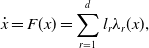
Reaction network dynamics can be modelled in various ways. For large molecule counts, ODEs are commonly used. Let $x(t)$
denote the species concentration vector, a time-dependent function in
$x(t)$
denote the species concentration vector, a time-dependent function in $\mathbb{R}^n$
. Then, it satisfies
$\mathbb{R}^n$
. Then, it satisfies
 \begin{equation} \dot{\kern-1pt x} = F(x) = \sum \limits _{r=1}^d l_r \lambda _r(x) , \end{equation}
where $\lambda _r(x)$
is the kinetics – the reaction rate of
$\lambda _r(x)$
is the kinetics – the reaction rate of $y_r \to y_r^{\prime }$
evaluated at
$y_r \to y_r^{\prime }$
evaluated at $x \in \mathbb{R}^n_{\geq 0}$
. Under the law of mass-action, the kinetics (mass-action kinetics) with rate constant
$x \in \mathbb{R}^n_{\geq 0}$
. Under the law of mass-action, the kinetics (mass-action kinetics) with rate constant $\kappa _r$
is written as
$\kappa _r$
is written as
 \begin{align} \lambda _r(x) = \kappa _r x^{y_r} =\kappa _r \prod \limits _{i=1}^n x_i^{y_{i,r}}. \end{align}
In contrast, in a system of small molecule counts, random fluctuations are significant, and thus CTMCs are used to model the dynamics of a RN. The species counts, denoted by $X_t$
, is a
$X_t$
, is a $\mathbb{Z}_{\geq 0}^n$
-valued CTMC, satisfying the equation
$\mathbb{Z}_{\geq 0}^n$
-valued CTMC, satisfying the equation
 \begin{align*} X(t) = X(0) + \sum _{r = 1}^d Y_{r} \left(\int _0^t \widetilde {\lambda }_{r} (X(s))\right) l_r, \end{align*}
where $\{Y_1,\ldots , Y_d\}$
is a set of i.i.d. Poisson processes with unit rates, and under the law of mass action, the kinetics in the stochastic modelling with rate constant
$\{Y_1,\ldots , Y_d\}$
is a set of i.i.d. Poisson processes with unit rates, and under the law of mass action, the kinetics in the stochastic modelling with rate constant $\kappa _r$
is given by
$\kappa _r$
is given by
 \begin{equation*}\widetilde {\lambda }_r(x) = \kappa _r \prod \limits _{i=1}^n \frac {x_i!}{(x_i - y_{i,r})!}1_{\{x_i\geq y_{i,r}\}}.\end{equation*}
Throughout this article, we denote by $(\mathcal{N}, \kappa )$
for an RN
$(\mathcal{N}, \kappa )$
for an RN $\mathcal{N}$
equipped with mass-action kinetics specified by the rate constant vector
$\mathcal{N}$
equipped with mass-action kinetics specified by the rate constant vector $\kappa$
.
$\kappa$
.
We conclude this subsection by introducing the definition of subnetworks.
Definition 2.2.
[
Reference Fontanil and Mendoza17
] Let $\mathcal{N}=(\mathcal{S},\mathcal{C},\mathcal{R})$
be an RN. Then, any reaction network
$\mathcal{N}=(\mathcal{S},\mathcal{C},\mathcal{R})$
be an RN. Then, any reaction network $\mathcal{N}'=(\mathcal{S}',\mathcal{C}',\mathcal{R}')$
is a subnetwork of
$\mathcal{N}'=(\mathcal{S}',\mathcal{C}',\mathcal{R}')$
is a subnetwork of $\mathcal{N}$
if
$\mathcal{N}$
if $\mathcal{R}' \subseteq \mathcal{R}$
(which implies both
$\mathcal{R}' \subseteq \mathcal{R}$
(which implies both $\mathcal{S}' \subseteq \mathcal{S}$
and
$\mathcal{S}' \subseteq \mathcal{S}$
and $\mathcal{C}' \subseteq \mathcal{C}$
).
$\mathcal{C}' \subseteq \mathcal{C}$
).
2.3. Langevin approximation
In practice, the CTMCs are typically studied through Monte Carlo simulations. Since the discrete stochastic simulations are generally computationally expensive, diffusion approximations, such as linear noise approximation (LNA) [Reference van Kampen57] and LA [Reference Kurtz35, Reference Kurtz36], are commonly used in numerical computation. Recently, a CLA [Reference Anderson, Higham, Leite and Williams4, Reference Leite and Williams40] was developed to address issues arising when the approximating process in LNA or LA reaches the boundary of the positive orthant. In this article, we focus on the identifiability of LA for stochastically modelled RNs.
As a frequently used diffusion approximation for stochastically modelled RNs, the LA is derived from the chemical Langevin equation (CLE) [Reference Gillespie54] and Itô-type SDE. The LA provides an accurate approximation for stochastic RNs up to the first hitting time of the boundary of the positive orthant and is preferred for capturing nonlinear effects in random fluctuations. Specifically, for an RN $(\mathcal{N}, \kappa )$
, the LA satisfies the following
$(\mathcal{N}, \kappa )$
, the LA satisfies the following $n$
-dimensional CLE:
$n$
-dimensional CLE:
 \begin{align} d X_t = A(X_t) dt + \sigma (X_t) dW_t, \end{align}
for all $t \gt 0$
with an initial value
$t \gt 0$
with an initial value $X_0 \in \mathbb{R}_{\gt 0}^n$
, where
$X_0 \in \mathbb{R}_{\gt 0}^n$
, where $A \colon \mathbb{R}^n \to \mathbb{R}^n$
is the drift vector,
$A \colon \mathbb{R}^n \to \mathbb{R}^n$
is the drift vector, $\sigma \colon \mathbb{R}^n \to \mathbb{R}^{n} \otimes \mathbb{R}^{n}$
is the diffusion coefficient and
$\sigma \colon \mathbb{R}^n \to \mathbb{R}^{n} \otimes \mathbb{R}^{n}$
is the diffusion coefficient and $W$
is a
$W$
is a $n$
-dimensional Brownian motion. In the context of LA for stochastic RNs,
$n$
-dimensional Brownian motion. In the context of LA for stochastic RNs, $A$
is given by
$A$
is given by
 \begin{equation} A_i(x) = \sum _{r=1}^d \Gamma _{i,r}\lambda _r(x) = \sum _{r=1}^d (y'_{i,r} - y_{i,r}) \kappa _r x^{y_r}, \quad i = 1,\ldots , n; \end{equation}
and $\sigma$
is given as the unique positive semi-definite square root (existence and uniqueness of square roots for any symmetric positive semi-definite matrix is well established; cf. [Reference Bhatia7].) of the diffusion matrix
$\sigma$
is given as the unique positive semi-definite square root (existence and uniqueness of square roots for any symmetric positive semi-definite matrix is well established; cf. [Reference Bhatia7].) of the diffusion matrix $B$
, with entries
$B$
, with entries
 \begin{equation} B_{i,j}(x)= (\sigma (x) \sigma (x)^{\intercal })_{i,j} = \sum _{r=1}^d \Gamma _{ir}\Gamma _{jr} \lambda _r(x) = \sum _{r = 1}^d (y'_{i,r} - y_{i,r}) (y'_{j,r} - y_{j,r}) \kappa _r x^{y_r}, \quad i, j = 1, \ldots , n. \end{equation}
Additionally, we recall that in (2.4) and (2.5), $\Gamma$
denotes the stoichiometric matrix, and
$\Gamma$
denotes the stoichiometric matrix, and $\lambda$
represents the mass-action kinetics defined in (2.2). In particular, when the initial state is important, we use the notation
$\lambda$
represents the mass-action kinetics defined in (2.2). In particular, when the initial state is important, we use the notation $X_t(x)$
to denote the solution to (2.3) with
$X_t(x)$
to denote the solution to (2.3) with $X_0 = x$
.
$X_0 = x$
.
3. Identifiability of RNs given dynamics
Although solutions to (2.3) may lack uniqueness and/or may explode in finite time, they are well defined and unique up to a stopping time when restricted to a bounded open subset of the positive orthant (see Subsection 5.1). This property enables us to explore the identifiability of RNs given their dynamics in this section. We begin with some definitions.
Definition 3.1.
Two stochastic processes $(X_t)_{t\geq 0},({X}'_t)_{t\geq 0}$
have the same distribution if they have the same finite dimensional distributions (fidis), which is denoted
$(X_t)_{t\geq 0},({X}'_t)_{t\geq 0}$
have the same distribution if they have the same finite dimensional distributions (fidis), which is denoted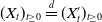 $(X_t)_{t\geq 0}\overset {d}{=}({X}'_t)_{t\geq 0}$
.
$(X_t)_{t\geq 0}\overset {d}{=}({X}'_t)_{t\geq 0}$
.
Definition 3.2.
Let $\mathcal{N} = (\mathcal{S}, \mathcal{C}, \mathcal{R})$
and
$\mathcal{N} = (\mathcal{S}, \mathcal{C}, \mathcal{R})$
and $\mathcal{N}' = (\mathcal{S}, \mathcal{C}', \mathcal{R}')$
be two RNs with the same set of species, where
$\mathcal{N}' = (\mathcal{S}, \mathcal{C}', \mathcal{R}')$
be two RNs with the same set of species, where $\mathcal{R} \neq \mathcal{R}'$
.
$\mathcal{R} \neq \mathcal{R}'$
.
-
• $\mathcal{N}$
is
reaction-identifiable
w.r.t. its SDE, if for every non-empty open bounded set
$U$
, for all initial states
$x\in U$
and distinct rate constant vectors
$\kappa , \kappa '\in \mathbb{R}_{\gt 0}^d$
, the corresponding stochastic processes, when stopped upon reaching the boundary of
$U$
, have different distributions starting from
$x$
.
$\mathcal{N}$
is
reaction-identifiable
w.r.t. its SDE, if for every non-empty open bounded set
$U$
, for all initial states
$x\in U$
and distinct rate constant vectors
$\kappa , \kappa '\in \mathbb{R}_{\gt 0}^d$
, the corresponding stochastic processes, when stopped upon reaching the boundary of
$U$
, have different distributions starting from
$x$
. -
•
$\mathcal{N}$
and
$\mathcal{N}'$
are
unconfoundable
w.r.t. their SDEs, if for every non-empty open bounded set
$U$
, for all initial states
$x\in U$
and rate constant vectors
$\kappa \in \mathbb{R}_{\gt 0}^d$
and
$\kappa '\in \mathbb{R}_{\gt 0}^{d'}$
, the corresponding stochastic processes, when stopped upon reaching the boundary of
$U$
, have different distributions starting from
$x$
.


The next theorem establishes sufficient and necessary conditions for the identifiability of RNs w.r.t. their SDEs. The proof is provided in Subsection 7.1.
Theorem 3.3.
Let $\mathcal{N} = (\mathcal{S}, \mathcal{C}, \mathcal{R})$
and
$\mathcal{N} = (\mathcal{S}, \mathcal{C}, \mathcal{R})$
and $\mathcal{N}' = (\mathcal{S}, \mathcal{C}', \mathcal{R}')$
be two RNs with the same set of species, where
$\mathcal{N}' = (\mathcal{S}, \mathcal{C}', \mathcal{R}')$
be two RNs with the same set of species, where $\mathcal{R} \neq \mathcal{R}'$
.
$\mathcal{R} \neq \mathcal{R}'$
.
-
(1)
$\mathcal{N}$
is reaction-identifiable w.r.t. its SDE if and only if for every source complex
$y\in \mathcal{C}$
, the set of vectors
(3.1)is linearly independent.
\begin{equation} \{(y'-y,(y' - y)\cdot (y' - y)^{\intercal }) \big | \, y\to y'\in \mathcal{R}\} \end{equation}
-
(2)
$\mathcal{N}$
and
$\mathcal{N}'$
are unconfoundable w.r.t. their SDEs if and only if they have different source complexes or share the same source complexes and for every source complex
$y \in \mathcal{C}$
,
$\mathrm{Cone}_{\mathcal{R}}(y) \cap \mathrm{Cone}_{\mathcal{R}'}(y) = \emptyset$
, where
(3.2)
\begin{align} \mathrm{Cone}_{\mathcal{R}}(y)\,:\!=\, \left \{\sum _{y\to y'\in \mathcal{R}}\alpha _{y\to y'}((y' - y),(y' - y)\cdot (y' - y)^{\intercal })\bigg |\, \alpha _{y\to y'}\gt 0\right \} \subseteq \mathbb{R}^n \times \mathbb{R}^n \otimes \mathbb{R}^n. \end{align}







Example 3.4 ([Reference Craciun and Pantea10], Fig. 3). Consider the following two RNs, where the first RN has reaction set $\mathcal{R}$
and the second has reaction set
$\mathcal{R}$
and the second has reaction set $\mathcal{R}'$
:
$\mathcal{R}'$
:
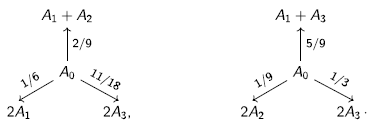
As shown in [ Reference Craciun, Tang and Feinberg11 ], these RNs are confoundable w.r.t. their ODEs. However, one finds that
 \begin{equation*} \mathrm{Cone}_{\mathcal{R}}(A_0) = \left \{\left (\begin{pmatrix} -\alpha _1-\alpha _2 -\alpha _3 \\[3pt] \alpha _1+2\alpha _2\\[3pt] \alpha _1\\[3pt] 2\alpha _3 \end{pmatrix},\begin{pmatrix} \alpha _1+\alpha _2+\alpha _3 & \quad\!\! -\alpha _1-2 \alpha _2 & \quad\!\! -\alpha _1 & \quad\!\! -\alpha _3 \\[3pt] -\alpha _1-2\alpha _2 & \quad\!\! \alpha _1+4\alpha _2 & \quad\!\! \alpha _1 & \quad\!\! 0\\[3pt] -\alpha _1 & \quad\!\! \alpha _1 & \quad\!\! \alpha _1& \quad\!\! 0 \\[3pt] -2\alpha _3 & \quad\!\! 0 & \quad\!\! 0 & \quad\!\! 4 \alpha _3 \end{pmatrix}\right ) \bigg |\, \alpha _1, \alpha _2, \alpha _3 \gt 0 \right \} , \end{equation*}
while
 \begin{equation*} \mathrm {Cone}_{\mathcal{R'}}(A_0) = \left \{\left (\begin{pmatrix} -\alpha _1-\alpha _2 -\alpha _3 \\[3pt] \alpha _1\\[3pt] 2\alpha _2\\[3pt] \alpha _1+2\alpha _3 \end{pmatrix},\begin{pmatrix} \alpha _1+\alpha _2+\alpha _3 & \quad\!\! -\alpha _1 & \quad\!\! -2\alpha _2 & \quad\!\! -\alpha _1-2\alpha _2\\[3pt] -\alpha _1 & \quad\!\! \alpha _1& \quad\!\! 0 & \quad\!\! \alpha _1 \\[3pt] -2\alpha _2 & \quad\!\! 0 & \quad\!\! 4\alpha _2& \quad\!\! 0 \\[3pt] -\alpha _1-2\alpha _2 & \quad\!\! \alpha _1& \quad\!\! 0 & \quad\!\! \alpha _2+4\alpha _3 \end{pmatrix}\right ) \bigg | \, \alpha _1,\alpha _2, \alpha _3 \gt 0 \right \} . \end{equation*}
It is easy to verify that $\mathrm{Cone}_{\mathcal{R}}(A_0) \cap \mathrm{Cone}_{\mathcal{R'}}(A_0) = \emptyset$
, since some coefficients are zero in one of the above matrices but positive in the other. As a result of Theorem
3.3
, these two RNs are unconfoundable w.r.t. their SDEs.
$\mathrm{Cone}_{\mathcal{R}}(A_0) \cap \mathrm{Cone}_{\mathcal{R'}}(A_0) = \emptyset$
, since some coefficients are zero in one of the above matrices but positive in the other. As a result of Theorem
3.3
, these two RNs are unconfoundable w.r.t. their SDEs.
Remark 3.5.
For a RN with mass-action kinetics, the rate constants associated with a source complex $y\in \mathcal{C}$
enter the CLE in both the drift and the diffusion terms,
$y\in \mathcal{C}$
enter the CLE in both the drift and the diffusion terms,
 \begin{align*} A(x) = \sum _{y\in \mathcal{C}}\sum _{y\to y'\in R} (y'-y)\,\kappa _{y\to y'}\, x^y, \qquad B(x) = \sum _{y\in \mathcal{C}}\sum _{y\to y'\in R} (y'-y)\cdot (y'-y)^{\intercal }\,\kappa _{y\to y'}\, x^y. \end{align*}
Hence, for each source complex $y\in C$
, the rate constants appear only through the finite family
$y\in C$
, the rate constants appear only through the finite family
 \begin{align*} \bigl ( y'-y,\,(y'-y)\cdot (y'-y)^{\intercal } \bigr ), \qquad y\to y'\in \mathcal{R}. \end{align*}
Theorem 3.3 shows that reaction identifiability of the SDE is equivalent to the linear independence of this family.
On the other hand, in the deterministic ODE setting, identifiability depends solely on the reaction vectors $y'-y$
[
Reference Craciun9
]. In contrast, in the SDE setting, the diffusion matrix contributes additional constraints through the terms
$y'-y$
[
Reference Craciun9
]. In contrast, in the SDE setting, the diffusion matrix contributes additional constraints through the terms $(y'-y)\cdot (y'-y)^{\intercal }$
, so that identifiability relies on the combined information from both drift and diffusion.
$(y'-y)\cdot (y'-y)^{\intercal }$
, so that identifiability relies on the combined information from both drift and diffusion.
For a general parametric SDE that does not arise from a reaction network, one may still ask whether the map $\theta \mapsto (A_\theta ,B_\theta )$
is injective. However, one cannot typically expect the existence of a canonical finite family of vectors whose linear independence characterises identifiability [
Reference Iacus27
]. The mass-action parametrisation of RNs is therefore crucial for the simple linear-algebraic criterion established in Theorem
3.3
.
$\theta \mapsto (A_\theta ,B_\theta )$
is injective. However, one cannot typically expect the existence of a canonical finite family of vectors whose linear independence characterises identifiability [
Reference Iacus27
]. The mass-action parametrisation of RNs is therefore crucial for the simple linear-algebraic criterion established in Theorem
3.3
.
3.1. Linear conjugacy
In the context of RNs, the concept of linear conjugacy was introduced in [Reference Johnston and Siegel29] for deterministically modelled RNs, borrowing ideas from dynamical systems theory [Reference Perko50]. This notion was further developed in subsequent works [Reference Johnston, Siegel and Szederkényi30, Reference Johnston, Siegel and Szederkényi31, Reference Nazareno, Eclarin, Mendoza and Lao46], among others. Earlier work on conjugacy in detailed balanced RNs can be found in [Reference Krambeck34]. Intuitively, two RNs are said to be linearly conjugated if there exists a linear mapping that transforms the trajectories of one system into those of the other. This property is of particular interest because qualitative features of mass-action systems, such as local stability, multistability, or persistence, are preserved under linear conjugacy. Our goal is to adapt the concept of linear conjugacy and extend the results of [Reference Johnston and Siegel29] to the stochastic setting.
Definition 3.6.
Let $(\mathcal{N}, \kappa )$
and
$(\mathcal{N}, \kappa )$
and $(\mathcal{N}', \kappa ')$
be two RNs with mass-action kinetics, that share a common set of species and
$(\mathcal{N}', \kappa ')$
be two RNs with mass-action kinetics, that share a common set of species and $\mathcal{R} \neq \mathcal{R}'$
.
$\mathcal{R} \neq \mathcal{R}'$
.
-
•
$(\mathcal{N}, \kappa )$
and
$(\mathcal{N}', \kappa ')$
are
$C^k$
-conjugated
w.r.t. their SDEs, if there exists a
$C^k$
-diffeomorphism
$h \colon \mathbb{R}_{\gt 0}^n \to \mathbb{R}_{\gt 0}^n$
, such that for any bounded open set
$U \subseteq \mathbb{R}_{\gt 0}^n$
, and every
$x \in U$
,(3.3)where
\begin{align} h(X_{t \wedge \tau }(x)) \overset {d}{=} X'_{t \wedge \tau '} (h(x)), \end{align}
$X_{t \wedge \tau } (x)$
and
$X_{t\wedge \tau '}' (h(x))$
denotes the solution to the LAs for
$(\mathcal{N}, \kappa )$
and
$(\mathcal{N}',\kappa ')$
starting at
$x$
and
$h(x)$
respectively, up to stopping times defined as
(3.4)
\begin{align} \tau \,:\!=\, \inf \{t \gt 0, X_t (x) \notin U\}\quad \text{and} \quad \tau ' \,:\!=\, \inf \big \{t \gt 0, X_t'(h(x)) \notin h(U)\big \}. \end{align}
-
•
$(\mathcal{N}, \kappa )$
and
$(\mathcal{N}', \kappa ')$
are
linearly conjugated
w.r.t. their SDEs, if they are
$C^{\infty }$
-conjugated w.r.t. their SDEs and the diffeomorphism
$h$
is linear.


Analogous to [Reference Johnston and Siegel29], the following theorem provides a necessary and sufficient condition for the linear conjugacy of two distinct RNs that share the same set of species. The proof is deferred to Subsection 7.4.
Theorem 3.7.
Let $\mathcal{N}$
and
$\mathcal{N}$
and $\mathcal{N}'$
be two RNs that share a common set of species and
$\mathcal{N}'$
be two RNs that share a common set of species and $\mathcal{R} \neq \mathcal{R}'$
. Then, there exist rate constant vectors
$\mathcal{R} \neq \mathcal{R}'$
. Then, there exist rate constant vectors $\kappa$
and
$\kappa$
and $\kappa '$
such that
$\kappa '$
such that $(\mathcal{N}, \kappa )$
and
$(\mathcal{N}, \kappa )$
and $(\mathcal{N}', \kappa ')$
are linearly conjugated w.r.t. their SDEs if and only if there exists a matrix
$(\mathcal{N}', \kappa ')$
are linearly conjugated w.r.t. their SDEs if and only if there exists a matrix $G$
of the form
$G$
of the form $G = DP$
, where
$G = DP$
, where $D$
is a positive diagonal matrix and
$D$
is a positive diagonal matrix and $P$
is a permutation matrix, such that
$P$
is a permutation matrix, such that $\mathcal{N}$
and
$\mathcal{N}$
and $\mathcal{N}'$
have the same complexes up to permutation by P, and such that for every source complex
$\mathcal{N}'$
have the same complexes up to permutation by P, and such that for every source complex $y$
of
$y$
of $\mathcal{N}$
it holds that:
$\mathcal{N}$
it holds that:
 \begin{align*} \mathrm {Cone}_{\mathcal{R}} (y) \cap \mathrm {Cone}^G_{\mathcal{R}'} (y) \neq \emptyset , \end{align*}
where $\mathrm {Cone}_{\mathcal{R}}$
is given by (3.2), and
$\mathrm {Cone}_{\mathcal{R}}$
is given by (3.2), and
 \begin{align*} \mathrm {Cone}^G_{\mathcal{R}'} (y) \,:\!=\, \left \{\sum _{y\to y'\in \mathcal{R}'}\alpha _{y\to y'} \left (G(y' - y),G (y' - y) \cdot (y' - y)^{\intercal } G^{\intercal }\right )\bigg |\, \alpha _{y\to y'}\gt 0\right \} . \end{align*}
Suppose the matrix $G$
in Theorem3.7 consists of only positive scaling. Then,
$G$
in Theorem3.7 consists of only positive scaling. Then, $G$
is a positive diagonal matrix, with diagonal entries
$G$
is a positive diagonal matrix, with diagonal entries $\{c_1, \ldots , c_n\} \subseteq \mathbb{R}_{\gt 0}$
. The following proposition describes the relationship between the rate constant vectors of linearly conjugate RNs w.r.t. their corresponding SDEs. The proof is presented in Subsection 7.5.
$\{c_1, \ldots , c_n\} \subseteq \mathbb{R}_{\gt 0}$
. The following proposition describes the relationship between the rate constant vectors of linearly conjugate RNs w.r.t. their corresponding SDEs. The proof is presented in Subsection 7.5.
Proposition 3.8.
Let $\mathcal{N} = (\mathcal{S}, \mathcal{C}, \mathcal{R})$
and
$\mathcal{N} = (\mathcal{S}, \mathcal{C}, \mathcal{R})$
and $\mathcal{N}' = (\mathcal{S}, \mathcal{C}', \mathcal{R}')$
be two RNs with the same set of species and source complexes. Suppose that for the rate constant vector
$\mathcal{N}' = (\mathcal{S}, \mathcal{C}', \mathcal{R}')$
be two RNs with the same set of species and source complexes. Suppose that for the rate constant vector $\kappa \in \mathbb{R}_{\gt 0}^d$
, there exists a positive vector
$\kappa \in \mathbb{R}_{\gt 0}^d$
, there exists a positive vector $\beta \in \mathbb{R}_{\gt 0}^{d'}$
and a positive diagonal matrix
$\beta \in \mathbb{R}_{\gt 0}^{d'}$
and a positive diagonal matrix $G$
with diagonal entries
$G$
with diagonal entries $\{c_1, \ldots , c_n\} \subseteq \mathbb{R}_{\gt 0}$
, such that for every source complex
$\{c_1, \ldots , c_n\} \subseteq \mathbb{R}_{\gt 0}$
, such that for every source complex $y$
:
$y$
:
 \begin{align} \sum _{y' \colon y\to y'\in \mathcal{R}}\kappa _{y\to y'}(y' - y) =\sum _{y' \colon y\to y'\in \mathcal{R}'}\beta _{y\to y'} G (y' - y) \end{align}
and
 \begin{align} \sum _{y' \colon y\to y'\in \mathcal{R}}\kappa _{y\to y'}(y' - y) \cdot (y' - y)^{\intercal } = \sum _{y' \colon y\to y'\in \mathcal{R}'} \beta _{y\to y'} G (y' - y) \cdot (y' - y)^{\intercal } G^{\intercal }. \end{align}
Then, $(\mathcal{N}, \kappa ')$
and
$(\mathcal{N}, \kappa ')$
and $(\mathcal{N}{{'}}, \kappa ')$
are linearly conjugated w.r.t. their SDEs, where for all
$(\mathcal{N}{{'}}, \kappa ')$
are linearly conjugated w.r.t. their SDEs, where for all $y \to y' \in \mathcal{R}'$
,
$y \to y' \in \mathcal{R}'$
,
 \begin{equation} \kappa '_{y\to y'} \,:\!=\, \beta _{y\to y'} c^y = \beta _{y\to y'} \prod _{j=1}^n c_j^{y_{j}}. \end{equation}
Remark 3.9.
Note that if we impose $G=Id$
the identity map, two different RNs
$G=Id$
the identity map, two different RNs $(\mathcal{N}, \kappa )$
and
$(\mathcal{N}, \kappa )$
and $(\mathcal{N}',\kappa ')$
are linearly conjugated with scaling matrix
$(\mathcal{N}',\kappa ')$
are linearly conjugated with scaling matrix $G = Id$
only if
$G = Id$
only if $\mathcal{N}$
and
$\mathcal{N}$
and $\mathcal{N}'$
are confoundable w.r.t. their SDEs.
$\mathcal{N}'$
are confoundable w.r.t. their SDEs.
Example 3.10. Consider the RNs:
 \begin{equation*}\mathcal{N}:\quad S_1\xrightarrow {\alpha } 3S_1 \quad \text{and } \quad \mathcal{N'}: \quad S_1\xrightarrow {\alpha '} 2S_1 .\end{equation*}
Following Theorem
3.3
, these RNs are not confoundable w.r.t. their SDEs since we cannot find $\alpha \gt 0$
and
$\alpha \gt 0$
and $\alpha '\gt 0$
such that:
$\alpha '\gt 0$
such that:
 \begin{equation*} 2\alpha = \alpha ' \quad \text{and } \quad 4\alpha = \alpha ' . \end{equation*}
In order for ( $\mathcal{N},\alpha$
) and (
$\mathcal{N},\alpha$
) and ( $\mathcal{N'},\alpha '$
) to be linearly conjugated, we need to find
$\mathcal{N'},\alpha '$
) to be linearly conjugated, we need to find $\alpha \gt 0, \alpha '\gt 0$
and
$\alpha \gt 0, \alpha '\gt 0$
and $c_1\gt 0$
such that
3.5
and
3.6
are verified, i.e.:
$c_1\gt 0$
such that
3.5
and
3.6
are verified, i.e.:
 \begin{equation*} 2\alpha = c_1 \alpha ' \quad \text{and } \quad 4\alpha = c_1^2 \alpha ' . \end{equation*}
It is verified for $\alpha = \alpha '$
and
$\alpha = \alpha '$
and $c_1=2$
. It follows that (
$c_1=2$
. It follows that ( $\mathcal{N},\alpha$
) and (
$\mathcal{N},\alpha$
) and ( $\mathcal{N'},\alpha '$
) are linearly conjugated.
$\mathcal{N'},\alpha '$
) are linearly conjugated.
Similarly as for reaction identifiability and confoundability (see Section 5), one can easily obtain the following lemma.
Lemma 3.11. If two RNs are not linearly conjugated w.r.t. their ODEs (see Definitions 3.1 and 3.2 of [ Reference Johnston and Siegel29 ]), then they are not linearly conjugated w.r.t. their SDEs.
4. Investigation of some special classes of RNs concerning identifiability
4.1. Special cases of reaction-identifiable RNs
-
(1) Consider RNs, which only consist of the following types of reactions:
with chemical species
\begin{equation*}S_i\rightarrow S_j, \quad S_i\rightarrow \emptyset , \quad \emptyset \rightarrow S_i ,\end{equation*}
$S_i$
,
$i=1,\ldots ,n$
.
For each complex, the associated reaction vectors are linearly independent, and it follows from [Reference Craciun and Pantea10, Theorem 3.2], that their corresponding RNs always have uniquely identifiable rate constants w.r.t. their ODEs and thus their SDEs. This property extends easily to k-unary chemical reaction networks [Reference Laurence and Robert39], with reactions of the types:
for
\begin{equation*}k_i S_i\rightarrow k_j S_j, \quad k_i S_i\rightarrow \emptyset , \quad \emptyset \rightarrow k_i S_i ,\end{equation*}
$1 \leq i \neq j \leq N$
, where
$k = (k_i)_{1\leq i \leq n} \in \mathbb{Z}^n_{\gt 0}$
.
-
(2) Simple RNs with only one species, have also uniquely identifiable rate constants w.r.t. the SDE, if and only if each source complex is a reactant in at most two reactions. Otherwise, the associated set of vectors in (3.1) will be constituted of three or more vectors in
$\mathbb{R}^2$
and will then be linearly dependent. -
(3) If each reaction in a RN has a distinct source complex, then the corresponding reaction vectors are automatically linearly independent, which in turn guarantees identifiability w.r.t. the ODE.




4.2. Counterexample
Given that RNs with complexes of molecularity of at most one are uniquely identifiable w.r.t. their SDEs, one might expect the same for RNs with reactants of molecularity at most one. The following examples show this is not the case.
Example 4.1. Consider the following RN:
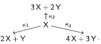
One can verify that the two sets of rate constant vectors $\kappa =(\kappa _1,\kappa _2,\kappa _3) = (2,7,5)$
and
$\kappa =(\kappa _1,\kappa _2,\kappa _3) = (2,7,5)$
and $\kappa ' = (\kappa _1',\kappa _2',\kappa _3') = (5,4,6)$
give the same SDE. Hence, this RN has not uniquely identifiable rate constants w.r.t. its SDE.
$\kappa ' = (\kappa _1',\kappa _2',\kappa _3') = (5,4,6)$
give the same SDE. Hence, this RN has not uniquely identifiable rate constants w.r.t. its SDE.
Note that if we remove the third chemical reaction namely $X\xrightarrow {\kappa _3} 4X+3Y$
, the set of vectors in (
3.1
) becomes linearly independent, which makes the RN having uniquely identifiable rate constants w.r.t. the ODE and then also w.r.t. the SDE.
$X\xrightarrow {\kappa _3} 4X+3Y$
, the set of vectors in (
3.1
) becomes linearly independent, which makes the RN having uniquely identifiable rate constants w.r.t. the ODE and then also w.r.t. the SDE.
5. Identifiability of RNs given generators
The proof of our main result, Theorem3.3, relies on establishing identifiability of RNs given generators. In this section, we introduce the formal notion of identifiability of RNs given their generators and present several supporting results that culminate in the proof of Theorem3.3.
5.1. More on SDEs
We start with introducing key concepts of SDEs relevant to this paper and refer the reader to, e.g. [Reference Ikeda and Watanabe28, Reference Øksendal48] for a more systematic study of the topic.
In general, the SDE (2.3) may not admit a unique solution for all $t \gt 0$
. One issue arises from the fact that the diffusion coefficient
$t \gt 0$
. One issue arises from the fact that the diffusion coefficient $\sigma (x) = \sqrt {B (x)}$
may fail to be Lipschitz continuous at the boundary of the positive orthant. In the one-dimensional case, this problem has been addressed in the seminal work [Reference Yamada and Watanabe61], which establishes the strong uniqueness for an SDE with an
$\sigma (x) = \sqrt {B (x)}$
may fail to be Lipschitz continuous at the boundary of the positive orthant. In the one-dimensional case, this problem has been addressed in the seminal work [Reference Yamada and Watanabe61], which establishes the strong uniqueness for an SDE with an $\alpha$
-Hölder continuous diffusion coefficient when
$\alpha$
-Hölder continuous diffusion coefficient when $\alpha \geq 1/2$
. However, in higher dimensions, where the equation under consideration is likely to reside, uniqueness is no longer guaranteed, as demonstrated in [Reference Swart52].
$\alpha \geq 1/2$
. However, in higher dimensions, where the equation under consideration is likely to reside, uniqueness is no longer guaranteed, as demonstrated in [Reference Swart52].
One possible remedy is to restrict the initial condition to lie strictly within the positive orthant. Even then, a second issue remains, that is the potential explosion of solutions in finite time. Since $\sigma (x)$
exhibits polynomial growth as
$\sigma (x)$
exhibits polynomial growth as $|x| \to \infty$
, it may blow up in finite time. This phenomenon is well understood in the one-dimensional setting [Reference Feller16] and has been generalised to higher dimensions in [Reference Khas’minskiĭ32]. We also note that the issue of (non-)explosion of RNs modelled by CTMCs has been investigated in [Reference Anderson, Cappelletti, Koyama and Kurtz2].
$|x| \to \infty$
, it may blow up in finite time. This phenomenon is well understood in the one-dimensional setting [Reference Feller16] and has been generalised to higher dimensions in [Reference Khas’minskiĭ32]. We also note that the issue of (non-)explosion of RNs modelled by CTMCs has been investigated in [Reference Anderson, Cappelletti, Koyama and Kurtz2].
Nevertheless, both the drift $A$
and the diffusion coefficient
$A$
and the diffusion coefficient $\sigma$
are Lipschitz continuous on compact subsets of the positive orthant and hence the following result holds, see, e.g. [Reference Ikeda and Watanabe28]. We begin with the standard definition of solutions to SDEs.
$\sigma$
are Lipschitz continuous on compact subsets of the positive orthant and hence the following result holds, see, e.g. [Reference Ikeda and Watanabe28]. We begin with the standard definition of solutions to SDEs.
Definition 5.1.
A stochastic process $X = (X_t)_{t \geq 0}$
is called
$X = (X_t)_{t \geq 0}$
is called
-
(1) a strong solution to (2.3), if it is adapted to the filtration generated by the Brownian motion
$W = (W_t)_{t \geq 0}$
in (2.3), and satisfies the following integral equation:
where the stochastic integral is interpreted in the Itô sense. A strong solution is called unique , if, whenever
\begin{align*} X_t - X_0 = \int _0^t A(X_s) ds + \int _0^t \sigma (X_s) d W_s, \end{align*}
$X$
and
$X'$
are any two strong solutions to (2.3) such that
$X_0 = X'_0$
a.s., then
$X_t = X_t'$
for all
$t \geq 0$
, a.s.
-
(2) a weak solution to (2.3), if there exists a probability space and a Brownian motion
$\widetilde {W} = (\widetilde {W}_t)_{t \geq 0}$
with
$\widetilde {W}_0 = 0$
, such that
$X$
is adapted to the filtration generated by
$\widetilde {W}$
and satisfies
where the stochastic integral is interpreted in the Itô sense. A weak solution is called unique (in law), if, whenever
\begin{align*} X_t - X_0 = \int _0^t A(X_s) ds + \int _0^t \sigma (X_s) d \widetilde {W}_s, \end{align*}
$X$
and
$X'$
are any two weak solutions to (2.3) such that
$X_0 \overset {d}{=} X'_0$
, then
$X_t \overset {d}{=} X'_t$
for all
$t \geq 0$
.


Theorem 5.2.
If we let $U \subseteq \mathbb{R}_{\gt 0}^n$
be a bounded open set and take an initial condition
$U \subseteq \mathbb{R}_{\gt 0}^n$
be a bounded open set and take an initial condition $x \in U$
, then (2.3) admits a unique strong solution up to the stopping time
$x \in U$
, then (2.3) admits a unique strong solution up to the stopping time $\tau = \inf \{t \gt 0\colon X_t (x) \notin U\}$
, and therefore also a unique weak solution.
$\tau = \inf \{t \gt 0\colon X_t (x) \notin U\}$
, and therefore also a unique weak solution.
This is sufficient for our investigation of identifiability. Moreover, the solution $(X_{t\wedge \tau }(x))_{t \geq 0}$
is a homogeneous Markov process. In the following, we introduce the concept of the infinitesimal generator for homogeneous Markov processes.
$(X_{t\wedge \tau }(x))_{t \geq 0}$
is a homogeneous Markov process. In the following, we introduce the concept of the infinitesimal generator for homogeneous Markov processes.
Definition 5.3 ([Reference Øksendal48], Definition 7.3.1). Let $(X_t)_{t \geq 0}$
be a homogeneous Markov process with state space
$(X_t)_{t \geq 0}$
be a homogeneous Markov process with state space $D \subseteq \mathbb{R}^n$
. The
infinitesimal generator
(or simply the generator) of
$D \subseteq \mathbb{R}^n$
. The
infinitesimal generator
(or simply the generator) of $X$
is an operator
$X$
is an operator $L$
on
$L$
on $C_c^{\infty } (D)$
, such that for all
$C_c^{\infty } (D)$
, such that for all $f \in C_c^{\infty } (D)$
and
$f \in C_c^{\infty } (D)$
and $x \in D$
,
$x \in D$
,
 \begin{align} L f(x) \,:\!=\, \lim _{t \to 0} \frac {\mathbb{E}[f(X_t(x))] - f(x)}{t}. \end{align}
For a general Markov process, the generator may not always exist—additional properties, such as strong continuity of the process, are required to ensure that the limit in (5.1) exists. In this paper, we focus on the LA for RNs, where the generator exists and takes the form in (5.2).
Then, [Reference Ethier and Kurtz13, Proposition 1.7 in Chapter 4] asserts the following theorem.
Theorem 5.4.
Let $(X_t)_{t \geq 0}$
be a Markov process with generator
$(X_t)_{t \geq 0}$
be a Markov process with generator $L$
. Then, it solves the
martingale problem
for
$L$
. Then, it solves the
martingale problem
for $L$
, namely, for every
$L$
, namely, for every $f \in C_c^{\infty } (\mathbb{R}^d)$
,
$f \in C_c^{\infty } (\mathbb{R}^d)$
,
 \begin{align*} M_t \,:\!=\, f(X_t) - \int _0^t L f(X_s) ds \end{align*}
is a martingale adapted to the filtration generated by $(X_t)_{t \geq 0}$
.
$(X_t)_{t \geq 0}$
.
If the Markov process $(X_t)_{t \geq 0}$
is the solution to an Itô equation (2.3), with locally Lipschitz continuous coefficients
$(X_t)_{t \geq 0}$
is the solution to an Itô equation (2.3), with locally Lipschitz continuous coefficients $A$
and
$A$
and $\sigma$
on
$\sigma$
on $\mathbb{R}_{\gt 0}^n$
, then its infinitesimal generator can be expressed as follows:
$\mathbb{R}_{\gt 0}^n$
, then its infinitesimal generator can be expressed as follows:
 \begin{equation} Lf(x) = \langle A(x), \nabla \rangle f{(x)}+{\frac {1}{2}} (\nabla ^{\intercal } \cdot B (x) \cdot \nabla ) f{(x)} = \sum _{i = 1}^n A_i(x)\frac {\partial }{\partial x_i}f(x)+\frac {1}{2}\sum _{i,j = 1}^n B_{i,j}(x)\frac {\partial ^2}{\partial x_i\partial x_j}f(x), \end{equation}
for all test functions $f\in C^{\infty }_c(\mathbb{R}_{\gt 0}^n)$
, cf. [Reference Øksendal48, Theorem 7.3.3].
$f\in C^{\infty }_c(\mathbb{R}_{\gt 0}^n)$
, cf. [Reference Øksendal48, Theorem 7.3.3].
Remark 5.5.
It is clear that drift and diffusion $A,B$
determine a generator of the form (5.2). Note that also the generator (5.2) uniquely determines
$A,B$
determine a generator of the form (5.2). Note that also the generator (5.2) uniquely determines $A,B$
, where we recall that
$A,B$
, where we recall that $B$
is symmetric. This can be seen, e.g. by considering test functions in
$B$
is symmetric. This can be seen, e.g. by considering test functions in $C_c^{\infty } (\mathbb{R}_{\gt 0}^n)$
that equal
$C_c^{\infty } (\mathbb{R}_{\gt 0}^n)$
that equal $x_i$
or
$x_i$
or $x_ix_j$
on a bounded open set inside
$x_ix_j$
on a bounded open set inside $\mathbb{R}_{\gt 0}^n$
[Reference Ethier and Kurtz13].
$\mathbb{R}_{\gt 0}^n$
[Reference Ethier and Kurtz13].
The following theorem, concerning the equivalence of martingale problems and SDEs, was first established in [Reference Stroock and Varadhan51] and further studied in [Reference Kurtz38]. The equivalence is given in terms of existence of SDEs through a weak solution, i.e. a filtered probability space and stochastic process that satisfies the SDE in its integral form [Reference Øksendal48, Section 5.5].
Theorem 5.6.
A stochastic process $(X_t)_{t \geq 0}$
is a solution to the martingale problem for
$(X_t)_{t \geq 0}$
is a solution to the martingale problem for $L$
of the form (5.2), if and only if it is a weak solution to (2.3).
$L$
of the form (5.2), if and only if it is a weak solution to (2.3).
Example 5.7. In order to exemplify notation, we again consider Example 1.1 :
 \begin{equation*}2S\xleftarrow {1}\emptyset \xrightarrow {4}S\xrightarrow {1} \emptyset \xrightarrow {2}3S , \end{equation*}
 \begin{equation*}2S\xleftarrow {4}\emptyset \xrightarrow {1}S \xrightarrow {1} \emptyset \xrightarrow {1}3S .\end{equation*}
The stoichiometric matrix is a row vector: $\Gamma = ( 2,1,-1,3)$
, which simplifies the calculation of both the drift vector and the diffusion matrix, that are
$\Gamma = ( 2,1,-1,3)$
, which simplifies the calculation of both the drift vector and the diffusion matrix, that are $A(x)=12-x$
and
$A(x)=12-x$
and $ B(x)=x+26$
for all
$ B(x)=x+26$
for all $x \in \mathbb{R}_{\gt 0}$
. Therefore, the LA for the RN is
$x \in \mathbb{R}_{\gt 0}$
. Therefore, the LA for the RN is
 \begin{align*} d X_t = (12 - X_t) dt + \sqrt {X_t + 26} d W_t; \end{align*}
and the infinitesimal generator associated to the RN is
 \begin{align*} L f(x) = (12 - x) \frac {d}{d x} f(x) + \frac {1}{2} (x + 26) \frac {d^2}{d x^2} f(x). \end{align*}
5.2. Reaction identifiability and confoundability given generator
Definition 5.8.
Let $\mathcal{N} = (\mathcal{S}, \mathcal{C}, \mathcal{R})$
and
$\mathcal{N} = (\mathcal{S}, \mathcal{C}, \mathcal{R})$
and $\mathcal{N}' = (\mathcal{S}, \mathcal{C}', \mathcal{R}')$
be two RNs with the same set of species, where
$\mathcal{N}' = (\mathcal{S}, \mathcal{C}', \mathcal{R}')$
be two RNs with the same set of species, where $\mathcal{R} \neq \mathcal{R}'$
.
$\mathcal{R} \neq \mathcal{R}'$
.
-
•
$\mathcal{N}$
is
reaction-identifiable
w.r.t. its generator, if and only if for any distinct rate constant vectors
$\kappa , \kappa ' \in \mathbb{R}^d_{\gt 0}$
, the corresponding generators of their LAs are different.
-
•
$\mathcal{N}$
and
$\mathcal{N}'$
are
confoundable
w.r.t. their generators, if there do exist rate constant vectors
$\kappa \in \mathbb{R}^d_{\gt 0}$
and
$\kappa '\in \mathbb{R}^{d'}_{\gt 0}$
such that the corresponding generators of their LAs are identical, where
$d$
and
$d'$
denote the numbers of reactions in
$\mathcal{N}$
and
$\mathcal{N}'$
, respectively. Otherwise, we say that
$\mathcal{N}$
and
$\mathcal{N}'$
are
unconfoundable
w.r.t. their generators.


In analogy to [Reference Craciun and Pantea10], we have the following result, whose proof is deferred to Subsection 7.2.
Theorem 5.9.
Let $\mathcal{N} = (\mathcal{S}, \mathcal{C}, \mathcal{R})$
be an RN. The followings are equivalent.
$\mathcal{N} = (\mathcal{S}, \mathcal{C}, \mathcal{R})$
be an RN. The followings are equivalent.
-
(1)
$\mathcal{N}$
is reaction-identifiable w.r.t. its generator.
-
(2) There is a non-empty bounded open set
$U\subseteq \mathbb{R}^n_{\gt 0}$
, such that for all rate constant vectors
$\kappa \neq \kappa '\in \mathbb{R}^d_{\gt 0}$
the corresponding generators are different on
$C^{\infty }_c(U)$
. -
(3) For every source complex
$y\in \mathcal{C}$
, the set of vectors in (3.1) is linearly independent.


Remark 5.10.
If two RNs $\mathcal{N}$
and
$\mathcal{N}$
and $\mathcal{N}'$
are unconfoundable w.r.t. their generators, then an analogous of property (2) in Theorem
5.9
holds for all rate constant vectors
$\mathcal{N}'$
are unconfoundable w.r.t. their generators, then an analogous of property (2) in Theorem
5.9
holds for all rate constant vectors $\kappa \in \mathbb{R}^d_{\gt 0}$
and
$\kappa \in \mathbb{R}^d_{\gt 0}$
and $\kappa ' \in \mathbb{R}^{d'}_{\gt 0}$
; see Subsection 7.2
.
$\kappa ' \in \mathbb{R}^{d'}_{\gt 0}$
; see Subsection 7.2
.
Lemma 5.11. If an RN is reaction-identifiable w.r.t. its ODE, then this RN is also reaction-identifiable w.r.t. its generator.
Proof. Suppose an RN is reaction-identifiable w.r.t. its ODE. Then, according to [Reference Craciun and Pantea10, Theorem 3.2], for any source complex $y \in \mathcal{C}$
, the set
$y \in \mathcal{C}$
, the set $\{y' - y \colon y \to y' \in \mathcal{R}\}$
is linearly independent. This, in turn, implies that the set of vectors in (3.1) is also linearly independent. Therefore, the RN is also reaction-identifiable w.r.t. its generator by Theorem5.9.
$\{y' - y \colon y \to y' \in \mathcal{R}\}$
is linearly independent. This, in turn, implies that the set of vectors in (3.1) is also linearly independent. Therefore, the RN is also reaction-identifiable w.r.t. its generator by Theorem5.9.
However, the converse is not necessarily true, as demonstrated in the following example.
Example 5.12. Consider the following birth and death reaction network:
 \begin{equation*}\emptyset \xleftarrow {\kappa _1} S\xrightarrow {\kappa _2} 2S,\end{equation*}
which is used to describe the evolution of cancer cells apart from other applications in biology [ Reference Novozhilov, Karev and Koonin47 ].
There is only one source complex $y = S$
, and we have that the set of vectors defined in (
3.1
), i.e.
$y = S$
, and we have that the set of vectors defined in (
3.1
), i.e. $ \{ (1,1)^{\intercal }, (-1,1)^{\intercal }\}$
are linearly independent. Therefore, according to Theorem
5.9
, this RN is reaction-identifiable w.r.t. its generator. However, if we consider
$ \{ (1,1)^{\intercal }, (-1,1)^{\intercal }\}$
are linearly independent. Therefore, according to Theorem
5.9
, this RN is reaction-identifiable w.r.t. its generator. However, if we consider $(\kappa _1,\kappa _2) = (1.5,1)$
and
$(\kappa _1,\kappa _2) = (1.5,1)$
and $(\kappa _1',\kappa _2') = (2,1.5)$
, then both reaction rates yield the same ODE system:
$(\kappa _1',\kappa _2') = (2,1.5)$
, then both reaction rates yield the same ODE system:
 \begin{align*} \dot{\kern-1pt x} = x-1.5x = 1.5x-2x=-0.5x. \end{align*}
It follows that the RN is not reaction-identifiable w.r.t. its ODE.
Remark 5.13.
In Example 5.12
, $S$
is the only source complex in the RN, which has deficiency one. In fact, it is not hard to verify that a RN with a single source complex is reaction-identifiable w.r.t. its ODE if and only if it has deficiency zero. However, as demonstrated in Example 5.12
, having zero deficiency is only a sufficient but not necessary condition for reaction identifiability w.r.t. its generator.
$S$
is the only source complex in the RN, which has deficiency one. In fact, it is not hard to verify that a RN with a single source complex is reaction-identifiable w.r.t. its ODE if and only if it has deficiency zero. However, as demonstrated in Example 5.12
, having zero deficiency is only a sufficient but not necessary condition for reaction identifiability w.r.t. its generator.
If an RN is not reaction-identifiable w.r.t. its generator, then it remains non-reaction-identifiable even with adding additional reactions.
Lemma 5.14.
Suppose an RN $\mathcal{N}$
is not reaction-identifiable w.r.t. its generator. Then, for every reaction network
$\mathcal{N}$
is not reaction-identifiable w.r.t. its generator. Then, for every reaction network $\mathcal{N}'$
such that
$\mathcal{N}'$
such that $\mathcal{N}$
is a subnetwork of
$\mathcal{N}$
is a subnetwork of $\mathcal{N}'$
,
$\mathcal{N}'$
, $\mathcal{N}'$
is also not reaction-identifiable w.r.t. its generator.
$\mathcal{N}'$
is also not reaction-identifiable w.r.t. its generator.
Proof. $\mathcal{N}$
is not reaction-identifiable w.r.t. its generator so there exists two vectors of rate constants
$\mathcal{N}$
is not reaction-identifiable w.r.t. its generator so there exists two vectors of rate constants $\kappa ^1_{\mathcal{N}}$
and
$\kappa ^1_{\mathcal{N}}$
and $\kappa ^2_{\mathcal{N}}$
giving the same generator. For any
$\kappa ^2_{\mathcal{N}}$
giving the same generator. For any $\mathcal{N}'$
with
$\mathcal{N}'$
with $d' \geq d$
reactions such that
$d' \geq d$
reactions such that $\mathcal{N}$
is a subnetwork of
$\mathcal{N}$
is a subnetwork of $\mathcal{N}'$
, we consider the rate constant vectors
$\mathcal{N}'$
, we consider the rate constant vectors $\kappa ^1_{\mathcal{N}'} = (\kappa ^1_{\mathcal{N}},a)$
and
$\kappa ^1_{\mathcal{N}'} = (\kappa ^1_{\mathcal{N}},a)$
and $\kappa ^2_{\mathcal{N}'}=(\kappa ^2_{\mathcal{N}},a)$
where
$\kappa ^2_{\mathcal{N}'}=(\kappa ^2_{\mathcal{N}},a)$
where $a \in \mathbb{R}^{d-d'}$
. These two vectors give the same generator, and thus,
$a \in \mathbb{R}^{d-d'}$
. These two vectors give the same generator, and thus, $\mathcal{N}'$
is not reaction-identifiable w.r.t. its generator.
$\mathcal{N}'$
is not reaction-identifiable w.r.t. its generator.
5.3. Confoundability of RNs given generators
In the previous subsection, we consider a given RN and its generator.
In this subsection, we investigate the confoundability of RNs given the generator.
Theorem 5.15.
Two RNs $\mathcal{N} = (\mathcal{S}, \mathcal{C}, \mathcal{R})$
and
$\mathcal{N} = (\mathcal{S}, \mathcal{C}, \mathcal{R})$
and $\mathcal{N}' = (\mathcal{S}, \mathcal{C}', \mathcal{R}')$
are confoundable w.r.t. their generators if and only if they have the same source complexes and for every source complex
$\mathcal{N}' = (\mathcal{S}, \mathcal{C}', \mathcal{R}')$
are confoundable w.r.t. their generators if and only if they have the same source complexes and for every source complex $y\in \mathcal{C}$
,
$y\in \mathcal{C}$
, $\mathrm {Cone}_{\mathcal{R}}(y) \cap \mathrm {Cone}_{\mathcal{R}'}(y) \neq \emptyset$
, where
$\mathrm {Cone}_{\mathcal{R}}(y) \cap \mathrm {Cone}_{\mathcal{R}'}(y) \neq \emptyset$
, where $\mathrm {Cone}_{\mathcal{R}}(y)$
is given by (3.2).
$\mathrm {Cone}_{\mathcal{R}}(y)$
is given by (3.2).
The proof of Theorem5.15 can be found in Subsection 7.3.
Example 5.16. Consider the following two different RNs:
 \begin{equation*}S\xleftarrow {5}\emptyset \xrightarrow {1}4S, \quad S\xrightarrow {1}\emptyset , \end{equation*}
 \begin{equation*}2S\xleftarrow {3}\emptyset \xrightarrow {1}3S, \quad S\xrightarrow {1}\emptyset .\end{equation*}
Again both RNs give the same ODE
 \begin{equation*}\frac {ds}{dt}=9-s.\end{equation*}
Despite the RNs being different, there exists two sets of reaction rates for which the ODEs are the same. Hence, the RN structure cannot be distinguished from the ODE alone. This is called (ODE)-confoundable in [ Reference Craciun9 ]. Furthermore, both RNs also have their SDEs given by the same drift vector and diffusion matrix
 \begin{equation*}A(s)=9-s,\quad B(s)=s+21.\end{equation*}
These RNs are thus confoundable w.r.t. their generator. As the corresponding SDE is regular enough, we conclude that these RNs are confoundable w.r.t. the SDE.
Remark 5.17. As pointed out in [ Reference Szederkényi53 ], the confoundability of two RNs w.r.t. their ODEs does not necessarily require their source complexes to be identical. A counterexample in [ Reference Szederkényi53 ] is constructed by choosing special rate constants for reactions with the additional source complex, such that its contribution to the corresponding ODE vanishes. However, this does not apply in our case, as the contribution of each source complex to the diffusion matrix is nonzero and non-negative definite. For further details, we refer the reader to the proof in Subsection 7.3 .
Similar to Lemma 5.11, we state the following lemma.
Lemma 5.18. If two RNs are unconfoundable w.r.t. their ODEs, then they are unconfoundable w.r.t. their generators.
Not surprisingly, the converse of Lemma 5.18 does not hold, as demonstrated in Remark 5.17.
By the definition of the generator, and in a manner similar to Lemma 5.14, the following extension result holds.
Lemma 5.19.
Let $\mathcal{N}_1 = (\mathcal{S}, \mathcal{C}_1, \mathcal{R}_1)$
and
$\mathcal{N}_1 = (\mathcal{S}, \mathcal{C}_1, \mathcal{R}_1)$
and $\mathcal{N}_2 = (\mathcal{S}, \mathcal{C}_2, \mathcal{R}_2)$
be two RNs confoundable w.r.t. their generators and let
$\mathcal{N}_2 = (\mathcal{S}, \mathcal{C}_2, \mathcal{R}_2)$
be two RNs confoundable w.r.t. their generators and let $r\not \in \mathcal{R}_1,r\not \in \mathcal{R}_2$
. Then also the RNs obtained by adding reaction
$r\not \in \mathcal{R}_1,r\not \in \mathcal{R}_2$
. Then also the RNs obtained by adding reaction $r$
to both
$r$
to both $\mathcal{R}_1$
and
$\mathcal{R}_1$
and $\mathcal{R}_2$
are confoundable w.r.t. their generators.
$\mathcal{R}_2$
are confoundable w.r.t. their generators.
6. Conclusion
This work rigorously examines the identifiability of SDEs derived from biochemical RNs under mass-action kinetics. Focusing on the Langevin approximation, we establish necessary and sufficient conditions for the identifiability of rate constants and reaction network structures based on the generator of the corresponding SDEs. We demonstrate that identifiability in the stochastic setting is finer than in the deterministic model, and that distinct RNs can generate indistinguishable stochastic dynamics. The results have direct implications for parameter inference and model selection in systems biology, offering tools to detect when models or parameters are indistinguishable from data. Future directions include extending the analysis to reflected diffusions under CLAs, or using different kinetics.
Conversely, our identifiability analysis was carried out under the assumption that the complete reaction-network is known, and all species are observed. In practice, however, only a subset of species is typically observed, and it is therefore of practical interest to establish identifiability under partial observability. This problem is relatively well studied in the ODE setting for monomolecular RNs [Reference Gross, Harrington, Meshkat and Shiu22], and analogous questions can be addressed for SDE models as well. Moreover, observations are usually available only at discrete time points, where transition densities are rarely available in closed form (except in special cases), and, e.g. maximum-likelihood inference is both numerically and theoretically delicate [Reference Iacus27]. Finally, while identifiability is a necessary condition for parameter estimation, it is generally not sufficient.
7. Proofs
7.1. Proof of Theorem3.3
With Theorems5.9 and 5.15 in hand, the validity of Theorem3.3 reduces to establishing the following proposition.
Proposition 7.1.
Let $\mathcal{N} = (\mathcal{S}, \mathcal{C}, \mathcal{R})$
and
$\mathcal{N} = (\mathcal{S}, \mathcal{C}, \mathcal{R})$
and $\mathcal{N}' = (\mathcal{S}, \mathcal{C}', \mathcal{R}')$
be two RNs with the same set of species, where
$\mathcal{N}' = (\mathcal{S}, \mathcal{C}', \mathcal{R}')$
be two RNs with the same set of species, where $\mathcal{R} \neq \mathcal{R}'$
.
$\mathcal{R} \neq \mathcal{R}'$
.
-
(1)
$\mathcal{N}$
is reaction-identifiable w.r.t. its SDE if and only if
$\mathcal{N}$
is reaction-identifiable w.r.t. its generator.
-
(2)
$\mathcal{N}$
and
$\mathcal{N}'$
are unconfoundable w.r.t. their SDEs if and only if they are unconfoundable w.r.t. their generators.


Proof. (1) $\implies$
: Suppose that
$\implies$
: Suppose that $\mathcal{N}$
is not reaction-identifiable w.r.t. its generator. Then, there exists distinct rate constant vectors
$\mathcal{N}$
is not reaction-identifiable w.r.t. its generator. Then, there exists distinct rate constant vectors $\kappa$
and
$\kappa$
and $\kappa '$
in
$\kappa '$
in $\mathbb{R}^{d}_{\gt 0}$
associated with the same generator on some non-empty bounded open subset
$\mathbb{R}^{d}_{\gt 0}$
associated with the same generator on some non-empty bounded open subset $U$
. By Theorem5.6 – the equivalence of the martingale problem and the SDE – we know that the stochastic processes associated to
$U$
. By Theorem5.6 – the equivalence of the martingale problem and the SDE – we know that the stochastic processes associated to $\kappa$
and
$\kappa$
and $\kappa '$
are weak solutions to the same SDE. Additionally, using Theorem5.2, solutions to this SDE are unique in law up to the stopping time
$\kappa '$
are weak solutions to the same SDE. Additionally, using Theorem5.2, solutions to this SDE are unique in law up to the stopping time $\tau = \inf \{t \gt 0, X_{t} \notin U\}$
. That is,
$\tau = \inf \{t \gt 0, X_{t} \notin U\}$
. That is, $\kappa$
and
$\kappa$
and $\kappa '$
provide two RNs with the identical distribution when starting from the same initial state. Hence,
$\kappa '$
provide two RNs with the identical distribution when starting from the same initial state. Hence, $\mathcal{N}$
is not reaction-identifiable w.r.t. its SDE. In other words,
$\mathcal{N}$
is not reaction-identifiable w.r.t. its SDE. In other words, $\mathcal{N}$
is reaction-identifiable w.r.t. its generator whenever it is reaction-identifiable w.r.t. its SDE.
$\mathcal{N}$
is reaction-identifiable w.r.t. its generator whenever it is reaction-identifiable w.r.t. its SDE. $\impliedby$
: Suppose that
$\impliedby$
: Suppose that $\mathcal{N}$
is not reaction-identifiable w.r.t. its SDE, then there exists
$\mathcal{N}$
is not reaction-identifiable w.r.t. its SDE, then there exists $\kappa \neq \kappa ' \in \mathbb{R}^{d}_{\gt 0}$
such that the two stochastic processes
$\kappa \neq \kappa ' \in \mathbb{R}^{d}_{\gt 0}$
such that the two stochastic processes $(X_t)_{t \geq 0}$
and
$(X_t)_{t \geq 0}$
and $(X'_t)_{t \geq 0}$
associated to
$(X'_t)_{t \geq 0}$
associated to $(\mathcal{N},\kappa )$
and
$(\mathcal{N},\kappa )$
and $(\mathcal{N},\kappa ')$
have the same distribution, when stopped upon reaching the boundary of
$(\mathcal{N},\kappa ')$
have the same distribution, when stopped upon reaching the boundary of $U$
. Then, the corresponding generators coincide, as by Definition 5.3,
$U$
. Then, the corresponding generators coincide, as by Definition 5.3,
 \begin{align} L f(x) = \lim _{t \downarrow 0}\frac {\mathbb{E} [f(X_t (x))] - f(x)}{t} = \lim _{t \downarrow 0}\frac {\mathbb{E} [f(X'_t (x))] - f(x)}{t} = L' f(x), \end{align}
for any $x \in U$
, and test function
$x \in U$
, and test function $f \in C_c^{\infty } (U)$
. This ensures that
$f \in C_c^{\infty } (U)$
. This ensures that $\mathcal{N}$
is not reaction-identifiable w.r.t. its generator.
$\mathcal{N}$
is not reaction-identifiable w.r.t. its generator.
(2) $\implies$
: Suppose that
$\implies$
: Suppose that $\mathcal{N}$
and
$\mathcal{N}$
and $\mathcal{N}'$
are confoundable w.r.t. their generators. Then there exists
$\mathcal{N}'$
are confoundable w.r.t. their generators. Then there exists $\kappa \in \mathbb{R}^{d}_{\gt 0}$
and
$\kappa \in \mathbb{R}^{d}_{\gt 0}$
and $\kappa ' \in \mathbb{R}^{d'}_{\gt 0}$
, such that
$\kappa ' \in \mathbb{R}^{d'}_{\gt 0}$
, such that $(\mathcal{N},\kappa )$
and
$(\mathcal{N},\kappa )$
and $(\mathcal{N}',\kappa ')$
have same generator on some non-empty bounded open subset
$(\mathcal{N}',\kappa ')$
have same generator on some non-empty bounded open subset $U$
. By Theorem5.6 – the equivalence of the martingale problem and the SDE – we know that the stochastic processes associated to
$U$
. By Theorem5.6 – the equivalence of the martingale problem and the SDE – we know that the stochastic processes associated to $(\mathcal{N},\kappa )$
and
$(\mathcal{N},\kappa )$
and $(\mathcal{N}',\kappa ')$
are weak solutions to the same SDE, and therefore share the same law up to the stopping time
$(\mathcal{N}',\kappa ')$
are weak solutions to the same SDE, and therefore share the same law up to the stopping time $\tau = \inf \{t \gt 0, X_{t} \notin U\}$
due to Theorem5.2. This proves that
$\tau = \inf \{t \gt 0, X_{t} \notin U\}$
due to Theorem5.2. This proves that $\mathcal{N}$
and
$\mathcal{N}$
and $\mathcal{N}'$
are confoundable w.r.t. their SDEs. Therefore,
$\mathcal{N}'$
are confoundable w.r.t. their SDEs. Therefore, $\mathcal{N}$
and
$\mathcal{N}$
and $\mathcal{N}'$
are unconfoundable w.r.t. their generators, whenever, they are unconfoundable w.r.t. their SDEs.
$\mathcal{N}'$
are unconfoundable w.r.t. their generators, whenever, they are unconfoundable w.r.t. their SDEs. $\impliedby$
: Suppose that
$\impliedby$
: Suppose that $\mathcal{N}$
and
$\mathcal{N}$
and $\mathcal{N}'$
are confoundable w.r.t. their SDEs, then there exists
$\mathcal{N}'$
are confoundable w.r.t. their SDEs, then there exists $\kappa \in \mathbb{R}^{d}_{\gt 0}$
and
$\kappa \in \mathbb{R}^{d}_{\gt 0}$
and $\kappa ' \in \mathbb{R}^{d'}_{\gt 0}$
such that the two stochastic processes
$\kappa ' \in \mathbb{R}^{d'}_{\gt 0}$
such that the two stochastic processes $(X_t)_{t \geq 0}$
and
$(X_t)_{t \geq 0}$
and $(X'_t)_{t \geq 0}$
associated to
$(X'_t)_{t \geq 0}$
associated to $(\mathcal{N},\kappa )$
and
$(\mathcal{N},\kappa )$
and $(\mathcal{N}',\kappa ')$
have same distribution, when stopped upon reaching the boundary of
$(\mathcal{N}',\kappa ')$
have same distribution, when stopped upon reaching the boundary of $U$
. Thus, equation (7.1) holds for any
$U$
. Thus, equation (7.1) holds for any $x \in U$
, and test function
$x \in U$
, and test function $f \in C_c^{\infty } (U)$
. This ensures that
$f \in C_c^{\infty } (U)$
. This ensures that $\mathcal{N}$
and
$\mathcal{N}$
and $\mathcal{N}'$
are confoundable w.r.t. their generators. The proof of this proposition is complete.
$\mathcal{N}'$
are confoundable w.r.t. their generators. The proof of this proposition is complete.
7.2. Proof of Theorem5.9
We will need the following elementary fact.
Lemma 7.2.
Let $Y\subset \mathbb Z_{\ge 0}^n$
be a finite set and let
$Y\subset \mathbb Z_{\ge 0}^n$
be a finite set and let $v_y\in \mathbb R^m$
be vectors for
$v_y\in \mathbb R^m$
be vectors for $y\in Y$
. If
$y\in Y$
. If
 \begin{align*} \sum _{y\in Y} v_y\,x^y = 0 \qquad \text{for all } x\in U,\quad U\subseteq \mathbb R^n\text{ open}, \end{align*}
then $v_y=0$
for all
$v_y=0$
for all $y\in Y$
.
$y\in Y$
.
Proof. Each coordinate of $\sum _{y\in Y} v_y x^y$
is a polynomial in
$\sum _{y\in Y} v_y x^y$
is a polynomial in $(x_1,\ldots ,x_n)$
that vanishes on the open set
$(x_1,\ldots ,x_n)$
that vanishes on the open set $U\subseteq \mathbb R^n$
. Hence, it is the zero polynomial and all coefficients vanish [Reference Mityagin45].
$U\subseteq \mathbb R^n$
. Hence, it is the zero polynomial and all coefficients vanish [Reference Mityagin45].
Proof of Theorem
5.9. $(1)\implies (2)$
: Let
$(1)\implies (2)$
: Let $\mathcal{N}$
be an RN such that
$\mathcal{N}$
be an RN such that $(2)$
fails. Then, there exist rate constant vectors
$(2)$
fails. Then, there exist rate constant vectors $\kappa \neq \kappa '$
, whose corresponding generators coincide on a nonempty open set
$\kappa \neq \kappa '$
, whose corresponding generators coincide on a nonempty open set $U$
. Recall that the generators take the form (5.2). The fact that two generators coincide on
$U$
. Recall that the generators take the form (5.2). The fact that two generators coincide on $C_c^{\infty } (U)$
is equivalent to their coefficients
$C_c^{\infty } (U)$
is equivalent to their coefficients $A_i$
and
$A_i$
and $B_i$
, which are polynomials, coinciding on
$B_i$
, which are polynomials, coinciding on $U$
. Since a nonzero polynomial cannot vanish on a nonempty open set, it follows that the coefficients (and hence the generators) coincide on all of
$U$
. Since a nonzero polynomial cannot vanish on a nonempty open set, it follows that the coefficients (and hence the generators) coincide on all of $\mathbb{R}^n_{\gt 0}$
(resp. on
$\mathbb{R}^n_{\gt 0}$
(resp. on $C^\infty _c(\mathbb{R}^n_{\gt 0})$
), see Lemma 7.2. As a consequence,
$C^\infty _c(\mathbb{R}^n_{\gt 0})$
), see Lemma 7.2. As a consequence, $\mathcal{N}$
is not identifiable w.r.t. its generator; that is
$\mathcal{N}$
is not identifiable w.r.t. its generator; that is $(1)$
fails. This proves the implication
$(1)$
fails. This proves the implication $(1) \implies (2)$
.
$(1) \implies (2)$
.
Notice that in the above argument, we do not actually require the underlying RNs with rate constant vectors $\kappa$
and
$\kappa$
and $\kappa '$
to share the same network structure. Therefore, the proof still justifies Remark 5.10 without any modification.
$\kappa '$
to share the same network structure. Therefore, the proof still justifies Remark 5.10 without any modification. $(2) \implies (3)$
: Assume that on an open subset
$(2) \implies (3)$
: Assume that on an open subset $U$
as given the generators are different for all
$U$
as given the generators are different for all $\kappa \neq \kappa '$
, but that there is a source complex
$\kappa \neq \kappa '$
, but that there is a source complex $y \in \mathcal{C}$
such that the set of vectors
$y \in \mathcal{C}$
such that the set of vectors
 \begin{equation*}\left \{\left (y' - y,(y' - y)\cdot (y' - y)^{\intercal }\right ) \big | \, y\to y'\in \mathcal{R}\right \}\end{equation*}
is linearly dependent. Then, there exist some real numbers $\alpha _{y\to y'}$
, not all zero such that
$\alpha _{y\to y'}$
, not all zero such that
 \begin{align*} \left (\sum _{y' \colon y \to y'\in \mathcal{R}} \alpha _{y\to y'}(y' - y),\sum _{y' \colon y \to y'\in \mathcal{R}} \alpha _{y\to y'} (y' - y)\cdot (y' - y)^{\intercal } \right ) = 0. \end{align*}
Hence, we can choose rate constant vectors $\kappa ,\kappa ' \in \mathbb{R}^{d}_{\gt 0}$
such that
$\kappa ,\kappa ' \in \mathbb{R}^{d}_{\gt 0}$
such that $\kappa _{y \to y'}- \kappa '_{y \to y'} = \alpha _{y \to y'}$
for all coefficients of reactions
$\kappa _{y \to y'}- \kappa '_{y \to y'} = \alpha _{y \to y'}$
for all coefficients of reactions $y \to y'\in \mathcal{R}$
and
$y \to y'\in \mathcal{R}$
and $\kappa _{R} = \kappa '_{R} = 1$
for other reactions
$\kappa _{R} = \kappa '_{R} = 1$
for other reactions $R \in \mathcal{R}$
. Then, recalling (2.4), (2.5), and (5.2), for these rate constant vectors, with
$R \in \mathcal{R}$
. Then, recalling (2.4), (2.5), and (5.2), for these rate constant vectors, with $L$
and
$L$
and $L'$
denoting the generator with
$L'$
denoting the generator with $k$
and
$k$
and $k'$
, respectively,
$k'$
, respectively,
 \begin{align*} L f(x) - L' f(x) = & \sum _{y\to y'\in \mathcal{R}} \left \langle (y' - y)(\kappa _{y\to y'}-\kappa '_{y\to y'})x^y, \nabla \right \rangle f \\ & + \frac {1}{2} \sum _{y\to y'\in \mathcal{R}} \left (\nabla ^{\intercal } \cdot (y' - y)\cdot (y' - y)^{\intercal }(\kappa _{y\to y'}-\kappa '_{y\to y'}) x^y \cdot \nabla \right ) f = 0. \end{align*}
This contradicts with our assumption, and thus verifies $(2) \implies (3)$
.
$(2) \implies (3)$
. $(3) \implies (1)$
: Assume that for all source complexes
$(3) \implies (1)$
: Assume that for all source complexes $y \in \mathcal{C}$
the set of vectors
$y \in \mathcal{C}$
the set of vectors
 \begin{equation*}\left \{\left (y' - y,(y' - y)\cdot (y' - y)^{\intercal }\right ) \big | \, y\to y'\in \mathcal{R} \right \}\end{equation*}
is linearly independent. Let $\kappa ,\kappa '\in \mathbb{R}^d_{\gt 0}$
such that
$\kappa ,\kappa '\in \mathbb{R}^d_{\gt 0}$
such that $L f(x) - L' f(x) = 0$
, for all test functions
$L f(x) - L' f(x) = 0$
, for all test functions $f\in C^{\infty }_c(\mathbb{R}_{\gt 0}^n)$
and
$f\in C^{\infty }_c(\mathbb{R}_{\gt 0}^n)$
and $x \in R_{\gt 0}^n$
. In other words,
$x \in R_{\gt 0}^n$
. In other words,
 \begin{equation*}\sum _{y \in \mathcal{C}} \left (\sum _{y' \colon y\to y'\in \mathcal{R}}(y' - y)(\kappa _{y\to y'} - \kappa '_{y\to y'})x^y,\sum _{y' \colon y\to y'\in \mathcal{R}}(y' - y)\cdot (y' - y)^{\intercal }(\kappa _{y\to y'}-k'_{y\to y'})x^y \right )= 0,\end{equation*}
where the right-hand side is the zero-function $\mathbb{R}^n\to \mathbb{R}^{n}\times \mathbb{R}^n \otimes \mathbb{R}^n$
. This yields that
$\mathbb{R}^n\to \mathbb{R}^{n}\times \mathbb{R}^n \otimes \mathbb{R}^n$
. This yields that
 \begin{equation*}\sum _{y\in \mathcal{C}}x^y\sum _{y' \colon y\to y'\in \mathcal{R}} (\kappa _{y\to y'}-\kappa '_{y\to y'}) \left ((y' - y),(y' - y)\cdot (y' - y)^{\intercal }\right )= 0.\end{equation*}
Since these vectors are polynomials in $x$
vanishing on
$x$
vanishing on $\mathbb{R}^n_{\gt 0}$
, their polynomial coefficients must be zero. Therefore, for each source complex
$\mathbb{R}^n_{\gt 0}$
, their polynomial coefficients must be zero. Therefore, for each source complex $y\in \mathcal{C}$
,
$y\in \mathcal{C}$
,
 \begin{equation*} \sum _{y' \colon y\to y'\in \mathcal{R}}(\kappa _{y\to y'}-\kappa '_{y\to y'}) \left ((y' - y),(y' - y)\cdot (y' - y)^{\intercal }\right )= 0 . \end{equation*}
By the linear independence, we get that $\kappa _{y\to y'}-\kappa '_{y\to y'}=0$
. This concludes the proof of
$\kappa _{y\to y'}-\kappa '_{y\to y'}=0$
. This concludes the proof of $(3) \implies (1)$
. The proof of this theorem is complete.
$(3) \implies (1)$
. The proof of this theorem is complete.
7.3. Proof of Theorem5.15
First, note that the condition $\textrm {Cone}_{\mathcal{R}}(y)\cap \textrm {Cone}_{\mathcal{R}'}(y)\neq \emptyset$
for all
$\textrm {Cone}_{\mathcal{R}}(y)\cap \textrm {Cone}_{\mathcal{R}'}(y)\neq \emptyset$
for all $y\in \mathcal{C}\cup \mathcal{C}'$
implies that
$y\in \mathcal{C}\cup \mathcal{C}'$
implies that $\mathcal{N}$
and
$\mathcal{N}$
and $\mathcal{N}'$
have the same source complexes: if
$\mathcal{N}'$
have the same source complexes: if $y$
is not a source complex of
$y$
is not a source complex of $\mathcal{R}$
, then
$\mathcal{R}$
, then $\textrm {Cone}_{\mathcal{R}}(y)=\{0\}$
by convention on the empty sum (and similarly for
$\textrm {Cone}_{\mathcal{R}}(y)=\{0\}$
by convention on the empty sum (and similarly for $\mathcal{R}'$
), but the coefficients of the coordinates in
$\mathcal{R}'$
), but the coefficients of the coordinates in $\textrm {Cone}_{\mathcal{R}'}(y)\subset \mathbb{R}^n \otimes \mathbb{R}^n$
from (3.2) are positive, so the intersection is empty. That is the difference to the ODE case of the proof of [Reference Craciun and Pantea10, Theorem 4.4] that was remarked in [Reference Szederkényi53]. Thus, it suffices to prove the equivalence between generator confoundability and the cone condition.
$\textrm {Cone}_{\mathcal{R}'}(y)\subset \mathbb{R}^n \otimes \mathbb{R}^n$
from (3.2) are positive, so the intersection is empty. That is the difference to the ODE case of the proof of [Reference Craciun and Pantea10, Theorem 4.4] that was remarked in [Reference Szederkényi53]. Thus, it suffices to prove the equivalence between generator confoundability and the cone condition. $\implies$
: Assume
$\implies$
: Assume $\mathcal{N}$
and
$\mathcal{N}$
and $\mathcal{N}'$
are confoundable with respect to their generators. Then there exist rate constant vectors
$\mathcal{N}'$
are confoundable with respect to their generators. Then there exist rate constant vectors $\kappa \in \mathbb R^{|\mathcal{R}|}_{\gt 0}$
and
$\kappa \in \mathbb R^{|\mathcal{R}|}_{\gt 0}$
and $\kappa '\in \mathbb R^{|\mathcal{R}'|}_{\gt 0}$
such that, for all
$\kappa '\in \mathbb R^{|\mathcal{R}'|}_{\gt 0}$
such that, for all $x\in \mathbb R^n_{\gt 0}$
,
$x\in \mathbb R^n_{\gt 0}$
,
 \begin{equation} \begin{cases} \displaystyle \sum _{y\in \mathcal{C}\cup \mathcal{C}'} \Bigg ( \sum _{\substack {y':\,y\to y'\in \mathcal{R}}} (y'-y)\,\kappa _{y\to y'} - \sum _{\substack {y':\,y\to y'\in \mathcal{R}'}} (y'-y)\,\kappa '_{y\to y'} \Bigg )x^y = 0,\\[15pt] \displaystyle \sum _{y\in \mathcal{C}\cup \mathcal{C}'} \Bigg ( \sum _{\substack {y':\,y\to y'\in \mathcal{R}}} (y'-y)\cdot (y'-y)^{\intercal }\,\kappa _{y\to y'} - \sum _{\substack {y':\,y\to y'\in \mathcal{R}'}} (y'-y)\cdot (y'-y)^{\intercal }\,\kappa '_{y\to y'} \Bigg )x^y = 0. \end{cases} \end{equation}
Apply Lemma 7.2 to the first (with $m=n$
) and the second lines simultaneously. We obtain, for every
$m=n$
) and the second lines simultaneously. We obtain, for every $y\in \mathcal{C}\cup \mathcal{C}'$
,
$y\in \mathcal{C}\cup \mathcal{C}'$
,
 \begin{equation} \begin{cases} \displaystyle \sum _{\substack {y':\,y\to y'\in \mathcal{R}}} (y'-y)\,\kappa _{y\to y'} = \sum _{\substack {y':\,y\to y'\in \mathcal{R}'}} (y'-y)\,\kappa '_{y\to y'},\\[15pt] \displaystyle \sum _{\substack {y':\,y\to y'\in \mathcal{R}}} (y'-y)\cdot (y'-y)^{\intercal }\,\kappa _{y\to y'} = \sum _{\substack {y':\,y\to y'\in \mathcal{R}'}} (y'-y)\cdot (y'-y)^{\intercal }\,\kappa '_{y\to y'}. \end{cases} \end{equation}
Fix a source complex $y$
. The pair determined by the left-hand sides of (7.3) belongs to
$y$
. The pair determined by the left-hand sides of (7.3) belongs to $\textrm {Cone}_{\mathcal{R}}(y)$
by definition, while the equal pair determined by the right-hand sides belongs to
$\textrm {Cone}_{\mathcal{R}}(y)$
by definition, while the equal pair determined by the right-hand sides belongs to $\textrm {Cone}_{\mathcal{R}'}(y)$
. Hence,
$\textrm {Cone}_{\mathcal{R}'}(y)$
. Hence,
 \begin{align*} \textrm {Cone}_{\mathcal{R}}(y)\cap \textrm {Cone}_{\mathcal{R}'}(y)\neq \emptyset \qquad \text{for every source complex } y. \end{align*} $\impliedby$
: Assume now that
$\impliedby$
: Assume now that $\mathcal{N}$
and
$\mathcal{N}$
and $\mathcal{N}'$
have the same source complexes and that for each source complex
$\mathcal{N}'$
have the same source complexes and that for each source complex $y$
,
$y$
, $\textrm {Cone}_{\mathcal{R}}(y)\cap \textrm {Cone}_{\mathcal{R}'}(y)\neq \emptyset$
. For each such
$\textrm {Cone}_{\mathcal{R}}(y)\cap \textrm {Cone}_{\mathcal{R}'}(y)\neq \emptyset$
. For each such $y$
, choose an element of the intersection and corresponding positive rate subvectors
$y$
, choose an element of the intersection and corresponding positive rate subvectors $\kappa ^{(y)}$
(for reactions in
$\kappa ^{(y)}$
(for reactions in $\mathcal{R}$
with source
$\mathcal{R}$
with source $y$
) and
$y$
) and $\kappa '^{(y)}$
(for reactions in
$\kappa '^{(y)}$
(for reactions in $\mathcal{R}'$
with source
$\mathcal{R}'$
with source $y$
) such that
$y$
) such that
 \begin{equation} \begin{cases} \displaystyle \sum _{\substack {y':\,y\to y'\in \mathcal{R}}} (y'-y)\,\kappa ^{(y)}_{y\to y'} = \sum _{\substack {y':\,y\to y'\in \mathcal{R}'}} (y'-y)\,\kappa '^{(y)}_{y\to y'},\\[15pt] \displaystyle \sum _{\substack {y':\,y\to y'\in \mathcal{R}}} (y'-y)\cdot (y'-y)^{\intercal }\,\kappa ^{(y)}_{y\to y'} = \sum _{\substack {y':\,y\to y'\in \mathcal{R}'}} (y'-y)\cdot (y'-y)^{\intercal }\,\kappa '^{(y)}_{y\to y'}. \end{cases} \end{equation}
Define global rate constant vectors $\kappa \in \mathbb R^{|\mathcal{R}|}_{\gt 0}$
and
$\kappa \in \mathbb R^{|\mathcal{R}|}_{\gt 0}$
and $\kappa '\in \mathbb R^{|\mathcal{R}'|}_{\gt 0}$
by setting, for each reaction
$\kappa '\in \mathbb R^{|\mathcal{R}'|}_{\gt 0}$
by setting, for each reaction $y\to y'$
,
$y\to y'$
,
 \begin{align*} \kappa _{y\to y'} \,:\!=\, \kappa ^{(y)}_{y\to y'}, \qquad \kappa '_{y\to y'} \,:\!=\, \kappa ^{\prime (y)}_{y\to y'}. \end{align*}
This is well defined because each reaction has a unique source complex $y$
. Then, (7.4) implies (7.3) for every source complex
$y$
. Then, (7.4) implies (7.3) for every source complex $y$
. Multiplying (7.3) by
$y$
. Multiplying (7.3) by $x^y$
and summing over
$x^y$
and summing over $y$
yields (7.2) for all
$y$
yields (7.2) for all $x\in \mathbb R^n_{\gt 0}$
. Therefore,
$x\in \mathbb R^n_{\gt 0}$
. Therefore, $\mathcal{N}$
and
$\mathcal{N}$
and $\mathcal{N}'$
are confoundable with respect to their generators.
$\mathcal{N}'$
are confoundable with respect to their generators.
7.4. Proof of Theorem3.7
The proof is similar in structure to that of Theorem5.15. First, $(\mathcal{N}, \kappa )$
and
$(\mathcal{N}, \kappa )$
and $(\mathcal{N}', k')$
are linear conjugates w.r.t. their SDEs, if and only if there exists a linear mapping
$(\mathcal{N}', k')$
are linear conjugates w.r.t. their SDEs, if and only if there exists a linear mapping $h'(x) = G x$
, such that, for any bounded open subset
$h'(x) = G x$
, such that, for any bounded open subset $U \subseteq \mathbb{R}_{\gt 0}^n$
(3.3) holds. Applying the same reasoning as in Theorem5.15, we conclude that
$U \subseteq \mathbb{R}_{\gt 0}^n$
(3.3) holds. Applying the same reasoning as in Theorem5.15, we conclude that $\mathcal{N}$
and
$\mathcal{N}$
and $\mathcal{N}'$
must have the same source complexes to be linear conjugate. On the other hand, [Reference Johnston and Siegel29, Lemma 3.1] asserts the matrix
$\mathcal{N}'$
must have the same source complexes to be linear conjugate. On the other hand, [Reference Johnston and Siegel29, Lemma 3.1] asserts the matrix $G$
consists of at most positively scaling and reindexing coordinates. Additionally,
$G$
consists of at most positively scaling and reindexing coordinates. Additionally, $h'(X_{t \wedge \tau })$
is a Markov process solving the martingale problem for the generator
$h'(X_{t \wedge \tau })$
is a Markov process solving the martingale problem for the generator
 \begin{equation*} L^{h'} f(x) = \langle G A(x), \nabla \rangle f + (\nabla ^{\intercal } \cdot G B G^{\intercal } (x) \cdot \nabla ) f . \end{equation*}
Thus, (3.3) is equivalent to equations
 \begin{equation*} \begin{cases} & \left (\sum \limits _{y' \colon y\to y'\in \mathcal{R}}(y' - y) \kappa _{y\to y'} - \sum \limits _{y' \colon y\to y'\in \mathcal{R}'}G(y' - y)\kappa '_{y\to y'} \right ) x^y = 0, \\[15pt] & \left (\sum \limits _{y' \colon y\to y'\in \mathcal{R}} (y' - y)\cdot (y' - y)^{\intercal } \kappa _{y\to y'}-\sum \limits _{y' \colon y\to y'\in \mathcal{R}'}G(y' - y)\cdot (y' - y)^{\intercal }G^{\intercal } \kappa '_{y\to y'} \right ) x^y = 0, \end{cases} \end{equation*}
for every source complex $y$
and state
$y$
and state $x \in U$
, which holds if and only if
$x \in U$
, which holds if and only if $ \textrm {Cone}_{\mathcal{R}} (y) \cap \textrm {Cone}^{G}_{\mathcal{R}'} (y) \neq \emptyset$
. This completes the proof of this theorem.
$ \textrm {Cone}_{\mathcal{R}} (y) \cap \textrm {Cone}^{G}_{\mathcal{R}'} (y) \neq \emptyset$
. This completes the proof of this theorem.
7.5. Proof of Proposition 3.8
Let $U \subseteq \mathbb{R}_{\gt 0}^n$
be an arbitrary bounded open set. Let
$U \subseteq \mathbb{R}_{\gt 0}^n$
be an arbitrary bounded open set. Let $X_{t \wedge \tau } (x)$
and
$X_{t \wedge \tau } (x)$
and $X_{t\wedge \tau '}' (z)$
be solutions to the LAs for
$X_{t\wedge \tau '}' (z)$
be solutions to the LAs for $(\mathcal{N}, \kappa )$
and
$(\mathcal{N}, \kappa )$
and $(\mathcal{N}', \kappa ')$
, starting at
$(\mathcal{N}', \kappa ')$
, starting at $x \in U$
and
$x \in U$
and $z = h(x) \,:\!=\, G^{-1} x \in h(U)$
, respectively, up to stopping times given by (3.4). Thus, concerning (2.4), (2.5), employing Itô’s formula, and recalling that
$z = h(x) \,:\!=\, G^{-1} x \in h(U)$
, respectively, up to stopping times given by (3.4). Thus, concerning (2.4), (2.5), employing Itô’s formula, and recalling that $G$
is a diagonal matrix, we can write
$G$
is a diagonal matrix, we can write
 \begin{align*} f \big (h \big (X_{t\wedge \tau }(x)\big )\big ) & =\, f(z) + \sum _{i = 1}^n \int _0^{t\wedge \tau } \sum _{r = 1}^{d} c_i^{-1} (y'_{i,r} - y_{i,r} ) \kappa _r X_{t\wedge \tau }(x)^{y_r} f^{(i)} \big (h \big (X_{t\wedge \tau }(x)\big )\big ) \\ & \quad + \frac {1}{2}\sum _{i,j = 1}^n \int _0^{t\wedge \tau } \sum _{r = 1}^d c_i^{-1} c_j^{-1} (y'_{i,r} - y_{i,r}) (y'_{j,r} - y_{j,r}) \kappa _{r} X_{t\wedge \tau }(x)^{y_r} f^{(i, j)} \big (X_{t\wedge \tau }(x)\big ) + M_{t \wedge \tau }\\ & = \sum _{i = 1}^n \sum _{y \in \mathcal{C}} h \big (X_{t\wedge \tau }(x)\big )^{y} c^y \sum _{y' \colon y \to y' \in \mathcal{R}} c_i^{-1} \kappa _{y \to y'} (y'_{i} - y_{i} ) \frac {\partial }{\partial z_i} f^{(i)} \big (h \big (X_{t\wedge \tau }(x)\big )\big ) \\ & \quad +\frac {1}{2}\sum _{i,j = 1}^n \sum _{y \in \mathcal{C}} h \big (X_{t\wedge \tau }(x)\big )^y c^y \sum _{y' \colon y \to y' \in \mathcal{R}} c_i^{-1} c_j^{-1} \kappa _{y \to y'} (y_{i}' - y_{i}) (y_{j}' - y_{j}) f^{(i, j)} \big (X_{t\wedge \tau }(x)\big ) + M_{t \wedge \tau }, \end{align*}
where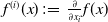 $f^{(i)} (x) \,:\!=\, \frac {\partial }{\partial x_i} f(x)$
,
$f^{(i)} (x) \,:\!=\, \frac {\partial }{\partial x_i} f(x)$
,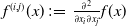 $f^{(i, j)} (x) \,:\!=\, \frac {\partial ^2}{\partial x_i \partial x_j} f(x)$
and
$f^{(i, j)} (x) \,:\!=\, \frac {\partial ^2}{\partial x_i \partial x_j} f(x)$
and $M_{t \wedge \tau }$
is a martingale. Therefore, the Markov process
$M_{t \wedge \tau }$
is a martingale. Therefore, the Markov process $h (X_{t \wedge \tau } (x)) = G^{-1} X_{t \wedge \tau } (x)$
solves the martingale problem for
$h (X_{t \wedge \tau } (x)) = G^{-1} X_{t \wedge \tau } (x)$
solves the martingale problem for $L^h$
given by
$L^h$
given by
 \begin{align*} L^h f (z) = & \sum _{i = 1}^n \sum _{y \in \mathcal{C}} z^{y} c^y \sum _{y' \colon y \to y' \in \mathcal{R}} c_i^{-1} \kappa _{y \to y'} (y'_{i} - y_{i} ) \frac {\partial }{\partial z_i} f(z) \\ & +\frac {1}{2}\sum _{i,j = 1}^n \sum _{y \in \mathcal{C}} z^y c^y \sum _{y' \colon y \to y' \in \mathcal{R}} c_i^{-1} c_j^{-1} \kappa _{y \to y'} (y_{i}' - y_{i}) (y_{j}' - y_{j}) \frac {\partial ^2}{\partial z_i\partial z_j}f(z), \end{align*}
for all $z = h(x) \in h(U)$
. On the other hand, formulas (3.5) and (3.6) suggest that for all
$z = h(x) \in h(U)$
. On the other hand, formulas (3.5) and (3.6) suggest that for all $i,j \in \{1,\ldots , n\}$
and any source complex
$i,j \in \{1,\ldots , n\}$
and any source complex $y$
,
$y$
,
 \begin{align*} c^y \sum _{y' \colon y\to y'\in \mathcal{R}} c_i^{-1} \kappa _{y\to y'}(y_i' - y_i) = \sum _{y' \colon y\to y'\in \mathcal{R}'} c^y \beta _{y\to y'} (y_i' - y_i) = \sum _{y' \colon y\to y'\in \mathcal{R}'} \kappa '_{y\to y'} (y_i' - y_i) \end{align*}
and
 \begin{align*} c^y \sum _{y' \colon y\to y'\in \mathcal{R}} c_i^{-1} c_j^{-1} \kappa _{y \to y'}(y_i' - y_j) \cdot (y'_j - y_j) = \sum _{y' \colon y\to y'\in \mathcal{R}'} \kappa '_{y\to y} (y_i' - y_i) \cdot (y_j' - y_j). \end{align*}
As a consequence, $L^h$
coincides with
$L^h$
coincides with $L'$
the generator for
$L'$
the generator for $X'_{t \wedge \tau '} (h(x)) = X'_{t \wedge \tau '} (z)$
 \begin{align*} L' f (z) = & \sum _{i = 1}^n \sum _{y \in \mathcal{C}} z^{y} \sum _{y' \colon y \to y' \in \mathcal{R}'} \!\!\kappa _{y \to y'}' (y'_{i} - y_{i}) \frac {\partial }{\partial z_i} f(z) +\frac {1}{2}\sum _{i,j = 1}^n \sum _{y \in \mathcal{C}} z^{y} \sum _{y' \colon y \to y' \in \mathcal{R}'} \!\!\kappa _{y \to y'}' (y_{i}' - y_{i}) \cdot (y_{j}' - y_{j}) \frac {\partial ^2}{\partial z_i\partial z_j}f(z). \end{align*}
This completes the proof of Proposition 3.8.
Acknowledgements
We thank Christian Mazza, Enrico Bibbona, Peter Pfaffelhuber and Jan van Waaij for helpful discussions.
Funding statement
LH was partially supported by the Swiss National Science Foundation grant (P2FRP2 188023).
Competing interests
The authors declare that they have no competing interests.
Data availability statement
A Julia implementation for assessing reaction identifiability, confoundability and linear conjugacy with respect to both ODEs and SDEs is available at: https://github.com/faullouis/Identifiability-of-SDEs-for-RNs.
See the Julia documentation at https://docs.julialang.org/ for a comprehensive user guide to the Julia programming language.

 Open access

