


1. Introduction
This paper considers shock propagation through a channel with an area discontinuity. This problem is one subset of the more general problem of wave reflection, transmission, and dissipation in channels. A large knowledge base on this problem exists in the acoustics literature (Lighthill Reference Lighthill1978; Fahy Reference Fahy2000; Lieuwen Reference Lieuwen2012), which is a useful starting point for the subsequent discussion. Assuming linear, one-dimensional(1-D) waves with no bulk flow, incident upon an area discontinuity with constant properties, approximate expressions can be developed for the wave reflection and transmission coefficients. These expressions are developed by assuming that the frequency is below the duct cutoff frequency (otherwise, multi-dimensional waves can be excited at the junction) and that the adjustment zone required for the multi-dimensional, evanescent disturbances to dissipate is small relative to an acoustic wavelength (Lighthill Reference Lighthill1978). By integrating the momentum and energy equations over this adjustment zone, it can be shown that the unsteady pressure and volume flow rate are approximately constant, leading to the resulting pressure reflection and transmission coefficients in terms of the area ratio $\alpha$
(Kinsler et al. Reference Kinsler, Frey, Coppens and Sanders2000):
$\alpha$
(Kinsler et al. Reference Kinsler, Frey, Coppens and Sanders2000):
 \begin{equation} T \equiv \frac {\text{transmitted wave amplitude}}{\text{incident wave amplitude}} = \frac {2\alpha }{\alpha + 1}, \end{equation}
 \begin{equation} R \equiv \frac {\text{reflected wave amplitude}}{\text{incident wave amplitude}} = \frac {\alpha - 1}{\alpha + 1}. \end{equation}
Mean flow and nonlinearity add additional effects. The integral approach described above can be readily generalized to include mean flow but also requires determining the pressure distribution across the control surfaces. This pressure distribution is itself controlled by whether the unsteady flow attaches to the bounding walls or separates (such as when flow transitions rapidly from smaller to larger cross-sectional area ducts). In either case, quasi-steady relations are typically invoked to develop analytical reflection and transmission coefficients. If there is no mean flow, unsteady flow separation causes the wave interaction problem to be intrinsically nonlinear (the acoustic wave dynamics themselves are linear, but the matching conditions are nonlinear) and dissipative, due to the conversion of some of the dilatational energy in the incident wave into rotational, vortical energy. In the presence of mean flow, the leading-order dissipation term is linear in disturbance amplitude. This wave dissipation phenomenon, including its nonlinear amplitude dependence, has been extensively characterized in the literature (Zinn Reference Zinn1970; Ingard & Sinhal Reference Ingard and Singhal1975).
The propagation of shocks through varying channels has receivsed significantly less treatment. This problem arises in several applications in which shocks move through channels, including rotating detonation engines (Kailasanath Reference Kailasanath, Gupta, De, Aggarwal, Kushari and Runchal2020), blast shelters (Cacoilo et al. Reference Cacoilo, Teixeira-Dias, Mourao, Belkassem, Vantomme and Lecompte2018) and supersonic wind tunnels (Gounko & Kavun Reference Gounko and Kavun2018). The shock problem introduces two important processes that are not present in the above described acoustic analyses – first, the wave dynamics themselves are intrinsically nonlinear and non-isentropic, and second, the disturbance length scale is very short. Prior work suggests that even for more complicated channels such as bends and bifurcations, the area ratio between the primary and secondary duct dominates the strength of the transmitted shock wave (Marty et al. Reference Marty, Daniel, Massoni, Biamino, Houas, Leriche and Jourdan2018).
Studies by Rudinger (Reference Rudinger1960) and Oppenheim, Urtiew & Stern (Reference Oppenhein, Urtiew and Stern1959) theoretically analysed wave transmission and reflection resulting from the shock–area change interaction; these works were later expanded upon by Salas (Reference Salas1991); we will utilize Rudinger’s method (Heilg & Igra Reference Heilg, Igra, Ben-Dor, Igra and Elperin2001) in this paper in calculating quasi-1-D approximations. These works can essentially be thought of as finite-amplitude generalizations of the work described above; i.e. they are quasi-1-D analyses that apply conservation principles to the flows upstream and downstream of the multi-dimensional adjustment zone in the immediate vicinity of the area change. As such, they neglect the multi-dimensional ‘near-field’ phenomena occurring near the area change. These can include vortices, oblique shock diamonds, and transverse wave reflections (Mendoza & Bowersox 2013). The nature of such phenomena, and the impact that they have on estimates of reflected and transmitted wave strength, are not understood.
There is some evidence that the impact of such phenomena on the farfield is fairly minor; Shoev et al. (Reference Shoev, Bondar, Khotyanovsky, Kudryavtsev, Maruta and Ivanov2012), for instance, noted a roughly 5 % discrepancy between the quasi-1-D calculations employed by Rudinger and Salas and the two-dimensional (2-D) averaged Euler equations when calculating the Mach numbers of transmitted shock waves through a microchannel. Similarly, Menina et al. (Reference Menina, Saurel, Zereq and Houas2011) observed that while these two methods showed understandable discrepancies in the immediate vicinity of the area change after the passage of the shock, these disagreements diminished sharply far beyond the area jump. However, these works do not answer the question of how general these results are and, even if they are generally true, why the discrepancies are small.
Furthermore, little is known about the energetics of this phenomenon. Travelling acoustic waves have the well-known ‘equi-partition’ property, where average energy density is evenly distributed between kinetic and internal energy associated with the ‘acoustic/compressional/dilatational’ disturbance. Even in the linear acoustic case, dilatational energy in the acoustic wave is not fully converted into the dilatational reflected and transmitted acoustic waves; this is manifested in the fact that the acoustic energy flux of the reflected and transmitted acoustic waves is less than that of the incident wave. Rather, as noted above, some irrotational, dilatational disturbance energy is converted into vortical disturbances where the energy is exclusively kinetic and manifested in rotational, incompressible disturbances (Chu & Kovasznay Reference Chu and Kovasznay1957; Lieuwen Reference Lieuwen2012). Some energy is also transferred into entropy disturbances if the wave interacts with a temperature variation. For the shock problem, although the types of disturbances resulting from this interaction are documented in the literature (Mendoza & Bowersox 2013), it is unknown how much energy is deposited in such disturbances and how much remains with the transmitted and reflected waves. These types of interactions between dilatational, vortical, and entropic disturbances are potentially much more significant in the shock–area change problem due to the much higher flow velocities behind the shock –which, via the Kutta condition (Crighton Reference Crighton1985), lead to vortical disturbances–as well as the intrinsically non-isentropic nature of shock waves. Menina et al. (Reference Menina, Saurel, Zereq and Houas2011) worked to address this gap by accounting for the transport of turbulent energy during the interaction between a weak shock and an abrupt area expansion, but this type of analysis has yet to be generalized to a broad range of incident shock strengths and area changes or to entropy disturbances.
Analytical tools have been developed to quantify energy flux and source terms in flow disturbances that can be brought to bear for this problem. Specifically, Myers (Reference Myers1991) has developed formal expressions that explicitly show the form of disturbance energy for arbitrary amplitude disturbances. This work has been generalized by Brear et al. (Reference Brear, Nicoud, Talei, Giauque and Hawkes2012) to include the effects of species transport and chemical reactions. These formulations are now routinely applied in thermo-acoustic problems (Meadows Reference Meadows1997; Weiczorek et al. Reference Weiczorek, Sensiau, Polifke and Nicoud2011), but this formalism has not yet been applied to the shock–area change problem, to the authors’ knowledge.
The primary goal of this work is to study the propagation of shocks through channels with discontinuous area changes. Within this larger goal, we have the following specific aims.
First, we wish to further understand the types of multi-dimensional, unsteady phenomena resulting from the shock–area change interaction and their impacts on the behaviour of the reflected and transmitted waves. Towards this end, we studied the reflection and transmission of shocks of various strengths through channels with various area changes using both computational fluid dynamics (CFD), which can account for 2-D transient effects, and quasi-1-D methods, which do not. These phenomena are characterized across five different ‘regimes’ governing the shock–area change interaction depending on the area ratio and incident Mach number. We also compare CFD and quasi-1-D theory, and show that they are in surprisingly good agreement, showcasing the viability of quasi-1-D methods to predict the asymptotic strength of reflected and transmitted shocks despite neglecting near-field phenomena. We utilize both inviscid and viscous calculations towards this end, and compare how the regimes are affected by viscosity.
Second, we perform an asymptotic analysis of the quasi-1-D expressions (which are generally implicit expressions) to derive explicit expressions for reflected and transmitted wave energy, as well as accumulation and dissipation of energy in the nearfield. The latter results are not only insightful in being presented in explicit form, but can also serve as boundary conditions for larger-scale calculations. Finally, we analyse the energetics of the interaction. To accomplish this, we use Myers’ expressions for disturbance energy (Myers Reference Myers1991), analyse the relative changes in dilatational energy associated with the area change, and examine the excited vortical and entropic disturbances.
2. Methods
This section is organized as follows. We begin by describing the aforementioned modelling approaches used in this work: the quasi-1-D theory and 2-D CFD. We then describe the methods used to analyse the energetics of the flow field in this problem. This includes a description of disturbance energy as it pertains to this problem, and the methods that we employ to decompose disturbance energy into three modes.
2.1. Modelling approaches
This subsection describes the quasi-1-D and 2-D methods used to analyse the flow field in this problem.
2.1.1. Quasi-1-D theory
(a) Diagram of wave patterns in parameter space. (b) Wave diagram for the case of a reflected shock wave and a transmitted shock and expansion wave (zone IIIa). A thick line indicates a shock; a thin lineindicates an expansion wave; a dashed line indicates a contact surface. Adapted from Salas (Reference Salas1991).

For this work, we used Rudinger’s method to perform quasi-1-D calculations of the flow field resulting from the shock–area change interaction. Rudinger’s method relies on formal application of the Rankine–Hugoniot relations, coupled with physical arguments on the nature of the contact surface, reflected shock wave and transmitted shock wave(s). In other words, before a solution can be obtained, one must first determine the structure of reflected and transmitted waves resulting from the interaction, through either experiment or appeals to physical principles to screen out physically unrealistic patterns. Also, as with most approaches relying on integral jump conditions, quasi-steady relations are used to match the wave characteristics of the incident, reflected and transmitted shocks far upstream and downstream of the area change where these disturbances are 1-D, implicitly neglecting the accumulation terms.
Results are a function of two parameters: the incident shock wave Mach number $M_i$
, and the ratio of upstream to downstream channel areas
$M_i$
, and the ratio of upstream to downstream channel areas $\alpha$
, as shown in figure 1. This parameter space is naturally divided into four quadrants separated by two lines: the space to the left of the vertical line (located at
$\alpha$
, as shown in figure 1. This parameter space is naturally divided into four quadrants separated by two lines: the space to the left of the vertical line (located at $\alpha$
= 1) represents area decreases, while the space to the right of this line represents area increases. Meanwhile, the space below the horizontal line (located at
$\alpha$
= 1) represents area decreases, while the space to the right of this line represents area increases. Meanwhile, the space below the horizontal line (located at $M_i= \left[ \left({(7 - \gamma ) + \sqrt {(7 - \gamma )^2 - 16(2 - \gamma )}}\right)/({4(2 - \gamma )})\right]^{1/2}\approx2.07$
for air) contains cases for which the flow behind the incident shock is subsonic, while the space above the horizontal line contains cases for which the flow behind the incident shock is supersonic. Within each quadrant are various zones corresponding to specific wave structures. One such pattern is shown in figure 1(b); this corresponds to the case of a single reflected and transmitted shock as well as an expansion wave transmitted from the area change. These structures are described next.
$M_i= \left[ \left({(7 - \gamma ) + \sqrt {(7 - \gamma )^2 - 16(2 - \gamma )}}\right)/({4(2 - \gamma )})\right]^{1/2}\approx2.07$
for air) contains cases for which the flow behind the incident shock is subsonic, while the space above the horizontal line contains cases for which the flow behind the incident shock is supersonic. Within each quadrant are various zones corresponding to specific wave structures. One such pattern is shown in figure 1(b); this corresponds to the case of a single reflected and transmitted shock as well as an expansion wave transmitted from the area change. These structures are described next.
Zone Ia corresponds to the case of a weak shock (by which we mean that the shocked flow is subsonic in the lab frame) and an area increase. In this case, the resulting interaction produces a reflected expansion wave and a transmitted shock. As the strength of the shock increases at a given area ratio, one moves into wave zone Ib. In this zone, the expansion wave is strong enough to produce sonic flow upstream of the area decrease. The resulting flow through the area decrease is choked, producing a standing shock wave within the area expansion, in addition to the waves described in the previous case. Further increasing the shock strength moves one into zone Ic. For this case, the pressure ratio across the area change is sufficiently strong to unchoke it, causing the standing shock to exit the area change as a second transmitted normal shock. If the incident shock is strengthened further still, then quadrant II is reached. For sufficiently large area ratios, the pattern corresponds to zone IIa, in which case the expansion wave in the previous case is no longer possible, due to the supersonic flow behind the incident shock, leaving only the two transmitted shocks. If the area ratio is too small, however, then the wave pattern becomes that of zone IIb, in which case the pressure ratio across the area change is too small to unchoke the area increase, resulting in a standing shock and a transmitted shock.
Quadrant IV corresponds to the case of a weak shock (again, one that induces subsonic flow in the lab frame) and a contracting duct. In this case, the resulting interaction produces a reflected and transmitted shock only. If the incident shock wave is strengthened, then the flow behind the area change is accelerated to sonic conditions. In this case, a transmitted expansion wave is generated in addition to the waves present in the previous case, resulting in a type IIIa pattern. For large enough area ratios, this pattern is also present in quadrant III. If, however, the area ratio is small enough, i.e. zone IIIb, then there is only a transmitted expansion wave and a transmitted shock.
To lay the foundation for the later section on approximate solutions derived via perturbation analysis around the small $(M_i - 1)$
limit for a calorically perfect gas, we summarize the key equations next. For a quasi-steady 1-D flow across an area discontinuity given by the upstream and downstream areas
$(M_i - 1)$
limit for a calorically perfect gas, we summarize the key equations next. For a quasi-steady 1-D flow across an area discontinuity given by the upstream and downstream areas $A_1$
and
$A_1$
and $A_2$
, one has the following governing equations:
$A_2$
, one has the following governing equations:
 \begin{equation} \rho _1 u_1 A_1 = \rho _2 u_2 A_2, \end{equation}
 \begin{equation} (p_1 + \rho _1 u_1^2)A_1 = (p_2 + \rho _2 u_2^2)A_2, \end{equation}
 \begin{equation} h_1 + \frac {u_1^2}{2} = \frac {c_1^2}{\gamma - 1} + \frac {u_1^2}{2} = \frac {c_2^2}{\gamma - 1} + \frac {u_2^2}{2}. \end{equation}
Equations (2.1)–(2.3) describe the conservation of mass, momentum and energy. The quantities $p$
,
$p$
, $\rho$
,
$\rho$
, $u$
,
$u$
, $c$
and
$c$
and $\gamma$
denote the pressure, density, velocity (in the frame of the shock), sound speed and specific heat ratio (assumed to be constant in this work), respectively. The final expression makes use of the ideal gas law to relate enthalpy
$\gamma$
denote the pressure, density, velocity (in the frame of the shock), sound speed and specific heat ratio (assumed to be constant in this work), respectively. The final expression makes use of the ideal gas law to relate enthalpy $h$
to sound speed. For conciseness, we define
$h$
to sound speed. For conciseness, we define
 \begin{equation} \begin{aligned} \delta \equiv \frac {\gamma - 1}{2} , \quad \kappa \equiv \frac {\gamma + 1}{2}. \end{aligned} \end{equation}
Rudinger’s method involves decomposing the fluid domain into zones separated by finite compression (shock) and expansion waves, contact surfaces, and the area change. To relate conditions across shock waves, the above conservation equations can be transformed into the Rankine–Hugoniot relations (Anderson Reference Anderson1990):
 \begin{equation} \frac {p_2}{p_1} = \frac {\gamma M_1^2 -\delta }{\kappa }, \end{equation}
 \begin{equation} \frac {\rho _2}{\rho _1} = \frac {u_1}{u_2} = \frac {\kappa M_1^2}{\delta M_1^2 + 1}, \end{equation}
 \begin{equation} M_2^2 = \frac {\delta M_1^2 + 1}{\gamma M_1^2 - \delta }. \end{equation}
It should be noted that the Mach number $M$
is, like
$M$
is, like $u$
, in the frame of the shock. For expansion waves, the following Riemann invariants were utilized:
$u$
, in the frame of the shock. For expansion waves, the following Riemann invariants were utilized:
 \begin{equation} J_+ = c + \delta u = {\rm const}, \end{equation}
 \begin{equation} J_- = c - \delta u = {\rm const}. \end{equation}
The above two relations hold for left- and right-moving isentropic waves, respectively. For isentropic state changes (i.e. changes throughout the expansion wave and area change, provided that there is no standing shock), the following equation was used:
 \begin{equation} \frac {p}{\rho ^{\gamma }} = {\rm const}. \end{equation}
This expression can be combined with the ideal gas law and appropriate conservation relations (i.e. the Riemann invariants for finite waves and conservation of mass/energy for the area change) to relate flow variables between two points. Finally, to relate conditions across a contact surface, we equated the pressure and velocity on either side. Thus although there is no explicit relation between other flow variables across the contact surface, they can still be related implicitly by fixing either pressure or velocity, solving for the corresponding velocity or pressure, and iterating this process until both pressure and velocity are continuous.
While the solution must generally be implemented computationally, Rudinger’s method can be solved explicitly in the weak shock limit using perturbation approaches. We detail the approach in Appendix A, and refer to these solutions later in interpreting computational results.
2.2. The 2-D computations
This subsection presents details of the simulations used to compute the 2-D domain, implemented with ANSYS Fluent 2022 R2. Fluent has robust tools for simulating shocks and has been employed toward this end in numerous works (Wen et al. Reference Wen, Karvounis, Walther, Ding and Yang2020; Janardhanraj, Abhishek & Jagadeesh Reference Janardhanraj, Abhishek and Jagadeesh2021). We employed the density-based solver with the Roe flux-difference splitting scheme. The temporal discretization used a second-order transient scheme with a time step such that the Courant number in the flow behind the incident shock is 0.5. The spatial discretization uses a second-order upwind scheme for flow variables, and a least squares cell-based scheme for gradient computation. Further information on these settings can be found in the Fluent User’s Guide (ANSYS Inc. 2022b ) and Theory Guide (ANSYS Inc. 2022a ). Structured geometry conforming mesh elements (quad cells) were used with uniform size 0.5 mm (1/20th the tube width); this size was determined from a mesh sensitivity study.
The width of the small duct was selected to be 10 mm, the width of the larger duct was determined from the area ratio, and both ducts were given lengths of at least 300 mm (i.e. 30 times the tube width) to capture the transmitted and reflected shocks far enough from the area change for them to be far removed from the near-field disturbances.
Shocks were generated by fixing the static pressure $p_i$
, total pressure
$p_i$
, total pressure $p_{t,i}$
, and total temperature
$p_{t,i}$
, and total temperature $T_{t,i}$
at the inlet to the appropriate values, which were calculated using the following equations:
$T_{t,i}$
at the inlet to the appropriate values, which were calculated using the following equations:
 \begin{equation} p_i = p_0\,\frac {\gamma M_i^2 - \delta }{\kappa }, \end{equation}
 \begin{equation} p_{t,i} = p_i\left (1 + \delta M_d^2\right )^{{\gamma }/{2\delta }}, \quad M_d = \frac {M_i^2 - 1}{\sqrt {(\delta M_i^2 + 1)(\gamma M_i^2 - \delta )}}, \end{equation}
 \begin{equation} T_{t,i} = T_i\left ( 1 +\delta M_d^2\right ), \quad T_i = T_0\, \frac {(\delta M_i^2 + 1)(\gamma M_i^2 - \delta )}{\kappa ^2 M_i^2}. \end{equation}
The above equations are merely re-expressions of the Rankine–Hugoniot relations (2.5)–(2.7) evaluated for the conditions upstream and downstream of the incident shock. Here, $p_0$
and
$p_0$
and $T_0$
represent the initial pressure and temperature in the domain, set at 1 atm and 300 K, respectively. All other surfaces were treated as walls with zero normal velocity and heat flux. This boundary condition is routinely used in problems of this type (Kailasanath Reference Kailasanath, Gupta, De, Aggarwal, Kushari and Runchal2020) and is appropriate because of the relatively short time of contact between the shock and post-shock gases and the wall. The exit boundary condition is unimportant provided that the duct is long enough (i.e. the shock can travel a sufficient distance to develop fully before interacting with the exit) and the pressure and velocity at the wall match that of the exit duct. The duct was initialized with quiescent, atmospheric air.
$T_0$
represent the initial pressure and temperature in the domain, set at 1 atm and 300 K, respectively. All other surfaces were treated as walls with zero normal velocity and heat flux. This boundary condition is routinely used in problems of this type (Kailasanath Reference Kailasanath, Gupta, De, Aggarwal, Kushari and Runchal2020) and is appropriate because of the relatively short time of contact between the shock and post-shock gases and the wall. The exit boundary condition is unimportant provided that the duct is long enough (i.e. the shock can travel a sufficient distance to develop fully before interacting with the exit) and the pressure and velocity at the wall match that of the exit duct. The duct was initialized with quiescent, atmospheric air.
Shock pressure reflection and transmission coefficients were extracted from these calculations, defined as (Rudinger Reference Rudinger1960)
 \begin{equation} T = \frac {p_4 - p_1}{p_3 - p_2}, \end{equation}
 \begin{equation} R = \frac {p_7 - p_3}{p_3 - p_2}, \end{equation}
where the subscripts denote zones in the channel, as summarized in figure 2.
Fluid zones in a channel for a type Ia pattern. Zones are numbered as follows: (1) the right-hand side of the area discontinuity not reached by the transmitted shock; (2) the left-hand side of the area discontinuity not reached by the incident shock; (3) the region upstream of the incident shock not reached by a reflected wave; (4) the region upstream of the transmitted shock not reached by the contact surface; (5) the region between the contact surface and the area discontinuity; (6) the region immediately downstream of the area discontinuity; and (7) the region between the reflected wave and the area discontinuity.

State variables of interest were taken to be the average in each of the zones in figure 2. Zone 4 was taken sufficiently far from the near-field zone that disturbances had returned to being 1-D. The CFD simulations were performed over a range of values for $M_i$
and
$M_i$
and $\alpha$
in all of the zones shown in figure 1.
$\alpha$
in all of the zones shown in figure 1.
Both viscous and inviscid computations were performed and compared. While inviscid calculations are quite standard in supersonic and shocked flow analyses, these comparisons are not only useful for assessing accuracy of inviscid calculations, but also lead to significant physical insight into controlling physics. The reason for this is that flow separation, and the accompanying separation of the approach flow viscous boundary layer into the core flow, is an inherent feature of this geometry. However, purely inviscid mechanisms – namely vortex sheet roll-up and baroclinic vorticity generation – generate significant vorticity in curved shock problems (Sun & Takayama Reference Sun and Takayama2003). Comparison of the vorticity budget in these two calculations provides some assessment of the relative role of viscous mechanisms of vorticity dynamics – i.e. reorganization of separating vorticity from boundary layers – versus inviscid ones. In the former case, because of the high Reynolds numbers of the shocked flows herein, we employed Fluent’s realizable $k\text{-}\varepsilon$
model with standard wall functions, in which the unsteady Reynolds-averaged Navier–Stokes (URANS) equations are solved with said eddy viscosity model (see the Theory Guide for further details; ANSYS Inc. 2022a
). A first-order discretization scheme was adopted for
$k\text{-}\varepsilon$
model with standard wall functions, in which the unsteady Reynolds-averaged Navier–Stokes (URANS) equations are solved with said eddy viscosity model (see the Theory Guide for further details; ANSYS Inc. 2022a
). A first-order discretization scheme was adopted for $k$
and
$k$
and $\varepsilon$
for these simulations. Inviscid calculations utilized Fluent’s inviscid model, which solves the unsteady Euler equations instead. In the viscous simulations, no-slip walls were imposed instead of slip walls. We report on the qualitative and quantitative aspects of both sets of calculations.
$\varepsilon$
for these simulations. Inviscid calculations utilized Fluent’s inviscid model, which solves the unsteady Euler equations instead. In the viscous simulations, no-slip walls were imposed instead of slip walls. We report on the qualitative and quantitative aspects of both sets of calculations.
2.3. Disturbance energy quantification
This subsection describes the approach used to quantify energy and energy flux during the shock–area change interaction. This energetics-based approach has been useful in several fields of study, particularly combustor noise (Brear et al. Reference Brear, Nicoud, Talei, Giauque and Hawkes2012) and combustion instabilities (Urbano et al. Reference Urbano, Selle, Staffelbach, Cuenot, Schmitt, Ducruix and Candel2016; Noiray & Denisov Reference Noiray and Denisov2017). Consider an energy equation of the form
 \begin{equation} \frac {\partial E}{\partial t} + \boldsymbol{\nabla} \boldsymbol{\cdot} {\boldsymbol {I}} = \phi, \end{equation}
where $\boldsymbol {I}$
represents the energy flux, and
$\boldsymbol {I}$
represents the energy flux, and $\phi$
represents energy sources/sinks. Furthermore, consider again the flow in the channel after the incident shock passes through the area change, as outlined in figure 2. Integrating over a control volume
$\phi$
represents energy sources/sinks. Furthermore, consider again the flow in the channel after the incident shock passes through the area change, as outlined in figure 2. Integrating over a control volume $V$
across the incident shock and making use of the divergence theorem, we have the relation
$V$
across the incident shock and making use of the divergence theorem, we have the relation
 \begin{equation} \begin{aligned} \frac {1}{A_L}\, \frac {\partial }{\partial t} \int _V E\, {\rm d}V &= \frac {1}{A_L} \int _V \frac {\partial E}{\partial t}\,{\rm d}V \\[5pt]
&= \frac {1}{A_L} \left [ \int _V \phi\, {\rm d} V - \int _S ({\boldsymbol {I}} \boldsymbol{\cdot} {\boldsymbol {n}})\,{\rm d}A \right ] \\[5pt]
&= \frac {1}{A_L} \int _V \phi\, {\rm d}V + I_{3,x} - I_{1,x} \\[5pt]
&\equiv I_i. \end{aligned} \end{equation}
\begin{equation} \begin{aligned} \frac {1}{A_L}\, \frac {\partial }{\partial t} \int _V E\, {\rm d}V &= \frac {1}{A_L} \int _V \frac {\partial E}{\partial t}\,{\rm d}V \\[5pt]
&= \frac {1}{A_L} \left [ \int _V \phi\, {\rm d} V - \int _S ({\boldsymbol {I}} \boldsymbol{\cdot} {\boldsymbol {n}})\,{\rm d}A \right ] \\[5pt]
&= \frac {1}{A_L} \int _V \phi\, {\rm d}V + I_{3,x} - I_{1,x} \\[5pt]
&\equiv I_i. \end{aligned} \end{equation}
In the above, $A_L$
represents the area on the left-hand (incident) side of the duct, while
$A_L$
represents the area on the left-hand (incident) side of the duct, while $I_{3,x}$
and
$I_{3,x}$
and $I_{1,x}$
represent
$I_{1,x}$
represent $x$
-components of the energy fluxes in zones 1 and 3 as defined in figure 2 (i.e. the unperturbed zone upstream of the area discontinuity and the zone upstream of the incident shock, respectively). We define
$x$
-components of the energy fluxes in zones 1 and 3 as defined in figure 2 (i.e. the unperturbed zone upstream of the area discontinuity and the zone upstream of the incident shock, respectively). We define $I_i$
to be the intensity of the incident shock, and define the intensities of the transmitted and reflected waves in the same manner. To evaluate
$I_i$
to be the intensity of the incident shock, and define the intensities of the transmitted and reflected waves in the same manner. To evaluate $E$
,
$E$
, $\boldsymbol {I}$
and
$\boldsymbol {I}$
and $\phi$
, we use the following expressions from (Myers Reference Myers1991):
$\phi$
, we use the following expressions from (Myers Reference Myers1991):
 \begin{equation} E \equiv \rho [h_T - h_{T0} - T_0(s - s_0)] - \rho _0{\boldsymbol {u}}_0 \boldsymbol{\cdot} ({\boldsymbol {u}} - {\boldsymbol {u}}_0) - (p - p_0), \end{equation}
 \begin{equation} {\boldsymbol {I}} \equiv (\rho {\boldsymbol {u}} - \rho _0 {\boldsymbol {u}}_0)[h_T - h_{T0} - T_0(s - s_0)] + \rho _0 {\boldsymbol {u}}_0(T - T_0)(s - s_0), \end{equation}
 \begin{equation} \phi \equiv (\rho {\boldsymbol {u}} - \rho _0 {\boldsymbol {u}}_0) \boldsymbol{\cdot} [\boldsymbol {\Omega } \times {\boldsymbol {u}} - \boldsymbol {\Omega }_0 \times {\boldsymbol {u}}_0 + (s - s_0)\,\boldsymbol{\nabla} T_0] - (s - s_0)\rho _0 {\boldsymbol {u}}_0 \boldsymbol{\cdot} \boldsymbol{\nabla} (T - T_0). \end{equation}
Here, $h_T$
,
$h_T$
, $s$
and
$s$
and $\Omega$
represent the total enthalpy, entropy and vorticity, respectively, while
$\Omega$
represent the total enthalpy, entropy and vorticity, respectively, while ${\boldsymbol {u}} \equiv (u, v)$
defines the fluid velocity vector.
${\boldsymbol {u}} \equiv (u, v)$
defines the fluid velocity vector. $()_0$
represents the unperturbed state of the fluid, taken in this case to be the state before the arrival of the incident shock. Note that these expressions do not include thermal and viscous diffusion. This is appropriate for the high Reynolds number, convectively dominated flows under consideration. Because the fluid is initially homogeneous and stationary, the source terms are identically zero. Hence the intensity of the incident shock equals the jump in energy flux before and after it.
$()_0$
represents the unperturbed state of the fluid, taken in this case to be the state before the arrival of the incident shock. Note that these expressions do not include thermal and viscous diffusion. This is appropriate for the high Reynolds number, convectively dominated flows under consideration. Because the fluid is initially homogeneous and stationary, the source terms are identically zero. Hence the intensity of the incident shock equals the jump in energy flux before and after it.
Equation (2.16) – with the given definitions of $E$
,
$E$
, $\boldsymbol {I}$
and
$\boldsymbol {I}$
and $\phi$
– is an extension of the familiar acoustic energy relation to arbitrary wave disturbance amplitudes. This enables us to define the power reflection and transmission coefficients
$\phi$
– is an extension of the familiar acoustic energy relation to arbitrary wave disturbance amplitudes. This enables us to define the power reflection and transmission coefficients
 \begin{equation} R_{\Pi} = R_I \equiv \frac {I_r}{I_i}, \end{equation}
 \begin{equation} T_{\Pi} = \frac {1}{\alpha }\,T_I \equiv \frac {I_t}{\alpha I_i}. \end{equation}
Here, $I_i \equiv |{\boldsymbol {I}}_i|$
,
$I_i \equiv |{\boldsymbol {I}}_i|$
, $I_t \equiv |{\boldsymbol {I}}_t|$
and
$I_t \equiv |{\boldsymbol {I}}_t|$
and $I_r \equiv |{\boldsymbol {I}}_r|$
are the incident, transmitted and reflected wave intensities, respectively. Partitioning the domain into the zones shown in figure 2, we define these as follows:
$I_r \equiv |{\boldsymbol {I}}_r|$
are the incident, transmitted and reflected wave intensities, respectively. Partitioning the domain into the zones shown in figure 2, we define these as follows:
 \begin{equation} {\boldsymbol {I}}_i \equiv {\boldsymbol {I}}_3, \quad {\boldsymbol {I}}_t \equiv {\boldsymbol {I}}_4, \quad {\boldsymbol {I}}_r \equiv {\boldsymbol {I}}_7 - {\boldsymbol {I}}_3. \end{equation}
Appendix B expands on the characteristics of Myers’ disturbance energy, and analyses them with respect to the finite-amplitude energy quantification approaches from Jenvey (Reference Jenvey1989) and Doak (Reference Doak1989).
Returning to the problem at hand, consider how to use these results for comparisons of quasi-1-D and 2-D results. There exists some zone before and after the area change where transient and 2-D effects persist; we refer to this as the near-field zone $V_n$
. Considering this zone, we have
$V_n$
. Considering this zone, we have
 \begin{equation} \begin{aligned} \frac {1}{A_L I_i}\int _{V_n} \frac {\partial E}{\partial t}\,{\rm d}V &= -\frac {1}{A_L I_i}\int _{\partial V_n} ({\boldsymbol {I}} \boldsymbol{\cdot} {\boldsymbol {n}})\,{\rm d}A \\ &= -\frac {1}{\alpha I_i}(I_4 - I_6). \end{aligned} \end{equation}
Define the accumulation coefficient $C_e$
to be the normalized disturbance energy flux transferred from the incident shock to disturbances other than the transmitted and reflected finite waves during the interaction:
$C_e$
to be the normalized disturbance energy flux transferred from the incident shock to disturbances other than the transmitted and reflected finite waves during the interaction:
 \begin{equation} \begin{aligned} C_e &\equiv \frac {A_LI_i - A_RI_t - A_LI_r}{A_LI_i} \\ &= 1 - T_{\Pi } - R_{\Pi }. \end{aligned} \end{equation}
Substituting (2.23) and (2.24) into the above relation produces
 \begin{equation} \begin{aligned} C_e &= \frac {1}{A_LI_i}\left [(A_LI_7 - A_RI_6) + \int _{V_n} \frac {\partial E}{\partial t}\,{\rm d}V \right ] \\ &= \frac {\mbox {flux through area change} + \mbox {accumulation in near-field zone}}{\mbox {incident disturbance energy}}. \end{aligned} \end{equation}
We will quantify this accumulation coefficient in the subsequent calculations. The above relations reveal insights into the relationship between quasi-1-D and general results. For instance, the only sources of energy flux between states 4 and 6 in the quasi-1-D theory are a contact surface and possible secondary transmitted waves. This contrasts with the general result, in which the transient, higher-dimensional behaviour in the near field may result in disturbance energy flux. This expression provides a convenient means to assess the magnitude of these discrepancies and their impact on the wave behaviour.
2.3.1. Decomposition into acoustic, vortical and entropic components
For this work, we wished to understand not only the amount of disturbance energy deposited into 2-D phenomena, but the distribution of this disturbance energy. A useful taxonomy for disturbances is to categorize them as acoustic/dilatational, vortical and entropy disturbances (Chu & Kovaznay Reference Chu and Kovasznay1957). These disturbances manifest themselves in the dilatation $\Lambda \equiv \boldsymbol{\nabla} \boldsymbol{\cdot} {\boldsymbol {u}}$
, vorticity
$\Lambda \equiv \boldsymbol{\nabla} \boldsymbol{\cdot} {\boldsymbol {u}}$
, vorticity $\Omega \equiv \boldsymbol{\nabla} \times {\boldsymbol {u}}$
and entropy
$\Omega \equiv \boldsymbol{\nabla} \times {\boldsymbol {u}}$
and entropy $s$
. We also calculated the instantaneous spatial distribution of the total disturbance energy flux
$s$
. We also calculated the instantaneous spatial distribution of the total disturbance energy flux $F \equiv \boldsymbol{\nabla} \boldsymbol{\cdot} {\boldsymbol {I}}$
. While these definitions are unique, note that these fields are not independent as they are in the linear case, but are strongly coupled through nonlinearities (Chu & Kovaznay Reference Chu and Kovasznay1957). In addition, evaluating their contribution to energy transfer becomes more nuanced in the finite-amplitude case because energy flux is a quadratic quantity and such disturbances are nonlinearly coupled (Lieuwen Reference Lieuwen2012). In order to provide insights into how the energy flux is distributed across disturbance modes, we also compared the disturbance energy flux to the corresponding space/time distribution of the dilatation, vorticity and entropy fields. This comparison can be done qualitatively (by visualizing the regions where large energy flux is coincident with regions of large disturbance amplitude of a given mode) or quantitatively by calculating the normalized correlation coefficient between fields as
$F \equiv \boldsymbol{\nabla} \boldsymbol{\cdot} {\boldsymbol {I}}$
. While these definitions are unique, note that these fields are not independent as they are in the linear case, but are strongly coupled through nonlinearities (Chu & Kovaznay Reference Chu and Kovasznay1957). In addition, evaluating their contribution to energy transfer becomes more nuanced in the finite-amplitude case because energy flux is a quadratic quantity and such disturbances are nonlinearly coupled (Lieuwen Reference Lieuwen2012). In order to provide insights into how the energy flux is distributed across disturbance modes, we also compared the disturbance energy flux to the corresponding space/time distribution of the dilatation, vorticity and entropy fields. This comparison can be done qualitatively (by visualizing the regions where large energy flux is coincident with regions of large disturbance amplitude of a given mode) or quantitatively by calculating the normalized correlation coefficient between fields as
 \begin{equation} \text{correlation coefficient} \equiv \frac {\sum _{i=0}^N(F_i - \bar {F})(\psi _i - \bar {\psi })}{\sqrt {\sum _{i=0}^N(F_i - \bar {F})^2 \sum _{i=0}^N(\psi _i - \bar {\psi })^2}}. \end{equation}
The above sums are evaluated over each point $i = 1, \ldots , N$
in the flow field. Here,
$i = 1, \ldots , N$
in the flow field. Here, $\psi$
represents one of the three variables noted above (
$\psi$
represents one of the three variables noted above ( $\Lambda$
,
$\Lambda$
, $\Omega$
and
$\Omega$
and $s$
), and the correlation coefficient was calculated at each instant in time, then time-averaged over a representative time window in which near-field effects are approximately quasi-steady. Therefore, although the flow is not statistically stationary for all time, these time averages are a useful and valid heuristic.
$s$
), and the correlation coefficient was calculated at each instant in time, then time-averaged over a representative time window in which near-field effects are approximately quasi-steady. Therefore, although the flow is not statistically stationary for all time, these time averages are a useful and valid heuristic.
We also analysed the disturbance energy density distribution using methods suggested by Jenvey (Reference Jenvey1989) and Doak (Reference Doak1989), which have been employed in past aero-acoustics studies (Unnikrishnan & Gaitonde Reference Unnikrishnan and Gaitonde2021) to analyse energy transfer between highly nonlinear vortical disturbances and far-field acoustic wave propagation. We perform this decomposition for disturbance energy density as follows. First, split the disturbance energy density into ‘internal’ and ‘kinetic’ energy contributions for reasons discussed later:
 \begin{equation} \begin{aligned} E &= \rho [h - h_{0} - T_0(s - s_0)] - (p - p_0) + \tfrac {1}{2}\rho {\boldsymbol {u}} \boldsymbol{\cdot} {\boldsymbol {u}} \\ &= e_D + \tfrac {1}{2}\rho {\boldsymbol {u}} \boldsymbol{\cdot} {\boldsymbol {u}}. \end{aligned} \end{equation}
Define the internal energy contribution $e_D$
and density
$e_D$
and density $\rho$
to be functions of
$\rho$
to be functions of $p$
and
$p$
and $s$
. Using the relations (Myers Reference Myers1991)
$s$
. Using the relations (Myers Reference Myers1991)
 \begin{equation} {\rm d}h = T\,{\rm d}S + \frac {1}{\rho }\,{\rm d}p, \quad {\rm d}p = \frac {c^2 \rho \beta T}{c_p}\,{\rm d}s + c^2\, {\rm d}\rho, \end{equation}
we differentiate with respect to time and apply the chain rule accordingly to obtain the following decomposition for $e_D$
:
$e_D$
:
 \begin{align} \frac {\partial e_D}{\partial t} &= \frac {\partial e_D}{\partial p} \bigg \rvert _{s = s_0} \frac {\partial p}{\partial t} + \frac {\partial e_D}{\partial p} \bigg \rvert _{p = p_0} \frac {\partial s}{\partial t}, \end{align}
 \begin{align} \frac {\partial e_D}{\partial p} \bigg \rvert _{s = s_0} &= \frac {1}{c^2}\left [h - h_0\right ], \end{align}
 \begin{align} \frac {\partial e_D}{\partial s} \bigg \rvert _{p = p_0} &= -\frac {\rho \beta T}{c_p}\left [\left (h - \frac {c_p}{\beta }\right ) - (h_0 - T_0s_0) - T_0\left (s - \frac {c_p}{\beta T}\right )\right ]. \end{align}
In the above relation, $\beta$
is the coefficient of thermal expansion
$\beta$
is the coefficient of thermal expansion $-(1/\rho )(\partial \rho /\partial T)_p$
, which evaluates to
$-(1/\rho )(\partial \rho /\partial T)_p$
, which evaluates to $\beta = 1/T$
for an ideal gas.
$\beta = 1/T$
for an ideal gas.
To handle the kinetic energy term, perform the following decomposition. First, following Jenvey and Doak, define the quantities
 \begin{equation} \boldsymbol{\nabla} \boldsymbol{\cdot} {\boldsymbol {u}}_{\Lambda } \equiv -\frac {1}{\gamma p}\,\frac {{\rm D}p}{{\rm D}t}, \quad \boldsymbol{\nabla} \boldsymbol{\cdot} {\boldsymbol {u}}_s \equiv \frac {1}{c_p}\,\frac {{\rm D}s}{{\rm D}t}. \end{equation}
Further defining these vector fields to be curl-free, define the curl-free velocity ${\boldsymbol {u}}_D$
as
${\boldsymbol {u}}_D$
as ${\boldsymbol {u}}_D \equiv {\boldsymbol {u}}_{\Lambda } + {\boldsymbol {u}}_s$
. The following relationships then hold:
${\boldsymbol {u}}_D \equiv {\boldsymbol {u}}_{\Lambda } + {\boldsymbol {u}}_s$
. The following relationships then hold:
 \begin{equation} \begin{aligned} \boldsymbol{\nabla} \boldsymbol{\cdot} {\boldsymbol {u}}_D &= \boldsymbol{\nabla} \boldsymbol{\cdot} {\boldsymbol {u}}_{\Lambda } + \boldsymbol{\nabla} \boldsymbol{\cdot} {\boldsymbol {u}}_s \\
&= -\frac {1}{\gamma p}\,\frac {{\rm D}p}{{\rm D}t} + \frac {1}{c_p}\,\frac {{\rm D}s}{{\rm D}t} \\ &= -\frac {1}{\rho }\,\frac {{\rm D}\rho }{{\rm D}t} \\ &= \boldsymbol{\nabla} \boldsymbol{\cdot} {\boldsymbol {u}}. \end{aligned} \end{equation}
\begin{equation} \begin{aligned} \boldsymbol{\nabla} \boldsymbol{\cdot} {\boldsymbol {u}}_D &= \boldsymbol{\nabla} \boldsymbol{\cdot} {\boldsymbol {u}}_{\Lambda } + \boldsymbol{\nabla} \boldsymbol{\cdot} {\boldsymbol {u}}_s \\
&= -\frac {1}{\gamma p}\,\frac {{\rm D}p}{{\rm D}t} + \frac {1}{c_p}\,\frac {{\rm D}s}{{\rm D}t} \\ &= -\frac {1}{\rho }\,\frac {{\rm D}\rho }{{\rm D}t} \\ &= \boldsymbol{\nabla} \boldsymbol{\cdot} {\boldsymbol {u}}. \end{aligned} \end{equation}
Finally, define the divergence-free velocity ${\boldsymbol {u}}_{\Omega }$
as
${\boldsymbol {u}}_{\Omega }$
as ${\boldsymbol {u}}_{\Omega } \equiv {\boldsymbol {u}} - {\boldsymbol {u}}_D$
, so that
${\boldsymbol {u}}_{\Omega } \equiv {\boldsymbol {u}} - {\boldsymbol {u}}_D$
, so that ${\boldsymbol {u}} = {\boldsymbol {u}}_{\Lambda } + {\boldsymbol {u}}_s + {\boldsymbol {u}}_{\Omega }$
. Given the above properties of
${\boldsymbol {u}} = {\boldsymbol {u}}_{\Lambda } + {\boldsymbol {u}}_s + {\boldsymbol {u}}_{\Omega }$
. Given the above properties of ${\boldsymbol {u}}_D$
, one has that
${\boldsymbol {u}}_D$
, one has that $\boldsymbol{\nabla} \boldsymbol{\cdot} {\boldsymbol {u}}_{\Omega }=\boldsymbol{\nabla} \boldsymbol{\cdot} {\boldsymbol {u}} - \boldsymbol{\nabla} \boldsymbol{\cdot} {\boldsymbol {u}}_D=0$
and
$\boldsymbol{\nabla} \boldsymbol{\cdot} {\boldsymbol {u}}_{\Omega }=\boldsymbol{\nabla} \boldsymbol{\cdot} {\boldsymbol {u}} - \boldsymbol{\nabla} \boldsymbol{\cdot} {\boldsymbol {u}}_D=0$
and $\boldsymbol{\nabla} \times {\boldsymbol {u}}_{\Omega } = \boldsymbol{\nabla} \times {\boldsymbol {u}} = \boldsymbol {\Omega }$
. Thus this procedure decomposes the velocity into components associated with pressure, vorticity and entropy as desired; we refer to
$\boldsymbol{\nabla} \times {\boldsymbol {u}}_{\Omega } = \boldsymbol{\nabla} \times {\boldsymbol {u}} = \boldsymbol {\Omega }$
. Thus this procedure decomposes the velocity into components associated with pressure, vorticity and entropy as desired; we refer to ${\boldsymbol {u}}_{\Lambda }$
,
${\boldsymbol {u}}_{\Lambda }$
, ${\boldsymbol {u}}_{\Omega }$
and
${\boldsymbol {u}}_{\Omega }$
and ${\boldsymbol {u}}_s$
as ‘acoustic/dilatational’, ‘vortical’ and ‘entropic’ velocity components, respectively. The procedure for solving for these fields is as follows.
${\boldsymbol {u}}_s$
as ‘acoustic/dilatational’, ‘vortical’ and ‘entropic’ velocity components, respectively. The procedure for solving for these fields is as follows.
-
(i) Solve the Poisson problem $\boldsymbol{\nabla} ^2 \phi$
=
$-\ {1}/{\rho }\ ({{\rm D}\rho }/{{\rm D}t})$
with the Neumann condition
$\boldsymbol{\nabla} \phi \boldsymbol{\cdot} \boldsymbol {n}$
=
${\boldsymbol {u}} \boldsymbol{\cdot} \boldsymbol {n}$
on the boundary for the velocity potential
$\phi$
. Inherent in this boundary condition is the assumption that
$\boldsymbol {u}$
is irrotational at the boundaries. This assumption is consistent with our inviscid calculations, which prevents the generation of vorticity at the walls. Determining boundary conditions for individual potentials for viscous no-slip walls poses numerous difficulties, such as the coupling between acoustic and vortical disturbances (Lieuwen Reference Lieuwen2012). As such, only the inviscid results are used in analysing these decompositions. Because of convecting vortical disturbances, it is also important to place the downstream boundary sufficiently far downstream.
$\boldsymbol{\nabla} ^2 \phi$
=
$-\ {1}/{\rho }\ ({{\rm D}\rho }/{{\rm D}t})$
with the Neumann condition
$\boldsymbol{\nabla} \phi \boldsymbol{\cdot} \boldsymbol {n}$
=
${\boldsymbol {u}} \boldsymbol{\cdot} \boldsymbol {n}$
on the boundary for the velocity potential
$\phi$
. Inherent in this boundary condition is the assumption that
$\boldsymbol {u}$
is irrotational at the boundaries. This assumption is consistent with our inviscid calculations, which prevents the generation of vorticity at the walls. Determining boundary conditions for individual potentials for viscous no-slip walls poses numerous difficulties, such as the coupling between acoustic and vortical disturbances (Lieuwen Reference Lieuwen2012). As such, only the inviscid results are used in analysing these decompositions. Because of convecting vortical disturbances, it is also important to place the downstream boundary sufficiently far downstream. -
(ii) Solve the Poisson problem
$\boldsymbol{\nabla} ^2 \phi _{\Lambda }$
=
$-({1}/{\gamma p})\ ({{\rm D}p}/{{\rm D}t})$
with the Neumann condition
$\boldsymbol{\nabla} \phi _{\Lambda } \boldsymbol{\cdot} \boldsymbol {n}$
=
${\boldsymbol {u}} \boldsymbol{\cdot} \boldsymbol {n}$
on the boundary. This boundary condition implicitly defines
${\boldsymbol {u}}_s \boldsymbol{\cdot} {\boldsymbol {n}}$
to be zero. -
(iii) Calculate
${\boldsymbol {u}}_{\Lambda }$
and
${\boldsymbol {u}}_{D}$
as
$\boldsymbol{\nabla} \phi _{\Lambda }$
and
$\boldsymbol{\nabla} \phi$
, respectively. -
(iv) Calculate
${\boldsymbol {u}}_s$
as
${\boldsymbol {u}}_{D}-{\boldsymbol {u}}_{\Lambda }$
. -
(v) Calculate
${\boldsymbol {u}}_{\Omega }$
as
$\boldsymbol {u}-{\boldsymbol {u}}_D$
.


Making use of the regular, rectangular grid for the domain, we discretized the above Poisson problems using second-order finite differencing, and solved the resulting system of equations using SciKit’s UMFPACK direct solver.
With this decomposition, we partition the kinetic energy accumulation in a similar manner:
 \begin{equation} \begin{aligned} \frac {\partial }{\partial t} \left (\frac {1}{2}\, \rho {\boldsymbol {u}} \boldsymbol{\cdot} {\boldsymbol {u}}\right ) &=\frac {{\boldsymbol {u}} \boldsymbol{\cdot} {\boldsymbol {u}} }{2}\, \frac {\partial \rho }{\partial t} + \rho {\boldsymbol {u}} \boldsymbol{\cdot} \frac {\partial {\boldsymbol {u}}}{\partial t} \\ &= \frac {({\boldsymbol {u}}_{\Lambda } + {\boldsymbol {u}}_{\Omega } + {\boldsymbol {u}}_s) \boldsymbol{\cdot} ({\boldsymbol {u}}_{\Lambda } + {\boldsymbol {u}}_{\Omega } + {\boldsymbol {u}}_s)}{2} \left (\frac {1}{c^2}\, \frac {\partial p}{\partial t} - \frac {\rho \beta T}{c_p}\, \frac {\partial s}{\partial t} \right ) \\ &\quad{}+ \rho ({\boldsymbol {u}}_{\Lambda } + {\boldsymbol {u}}_{\Omega } + {\boldsymbol {u}}_s) \boldsymbol{\cdot} \frac {\partial }{\partial t} ({\boldsymbol {u}}_{\Lambda } + {\boldsymbol {u}}_{\Omega } + {\boldsymbol {u}}_s). \end{aligned} \end{equation}
We now define the acoustic, vortical and entropic contributions to the disturbance energy density to be those terms that are strictly associated with the three fields, i.e. those associated with pure multiples of $\ {\partial p}/{\partial t}$
and/or
$\ {\partial p}/{\partial t}$
and/or ${{\boldsymbol {u}}}_{\boldsymbol {\Lambda }}$
,
${{\boldsymbol {u}}}_{\boldsymbol {\Lambda }}$
, ${\boldsymbol {u}}_{\boldsymbol {\Omega }}$
and
${\boldsymbol {u}}_{\boldsymbol {\Omega }}$
and $\ {\partial s}/{\partial t}$
and/or
$\ {\partial s}/{\partial t}$
and/or ${\boldsymbol {u}}_{{\boldsymbol {s}}}$
, respectively. In doing so, we expand on the methods of Jenvey and Doak by excluding combinations of such terms (
${\boldsymbol {u}}_{{\boldsymbol {s}}}$
, respectively. In doing so, we expand on the methods of Jenvey and Doak by excluding combinations of such terms ( ${\boldsymbol {u}}_s \boldsymbol{\cdot} {\boldsymbol {u}}_{\Lambda }$
, for instance) from these categories, and group them into four additional coupled terms. Thus we have the following definitions for each of the seven contributions to the disturbance energy accumulation
${\boldsymbol {u}}_s \boldsymbol{\cdot} {\boldsymbol {u}}_{\Lambda }$
, for instance) from these categories, and group them into four additional coupled terms. Thus we have the following definitions for each of the seven contributions to the disturbance energy accumulation $\dot {E} \equiv \partial {E}/\partial {t}$
:
$\dot {E} \equiv \partial {E}/\partial {t}$
:
 \begin{align} \dot {E}_{\Lambda } &\equiv \frac {1}{c^2}\left (h - h_0 + \frac {{\boldsymbol {u}}_{\Lambda } \boldsymbol{\cdot} {\boldsymbol {u}}_{\Lambda }}{2} \right )\frac {\partial p}{\partial t} + \rho {\boldsymbol {u}}_{\Lambda } \boldsymbol{\cdot} \frac {\partial {\boldsymbol {u}}_{\Lambda }}{\partial t}, \end{align}
 \begin{align} \dot {E}_{\Omega } &\equiv \rho {\boldsymbol {u}}_{\Omega } \boldsymbol{\cdot} \frac {\partial {\boldsymbol {u}}_{\Omega }}{\partial t}, \end{align}
 \begin{align} \dot {E}_s &\equiv -\frac {\rho \beta T}{c_p}\left (\left [h - \frac {c_p}{\beta }\right ] - (h_0 - T_0s_0) - T_0\left [s - \frac {c_p}{\beta T}\right ] + \frac {{\boldsymbol {u}}_s \boldsymbol{\cdot} {\boldsymbol {u}}_s}{2}\right ) \frac {\partial s}{\partial t} + \rho {\boldsymbol {u}}_s \boldsymbol{\cdot} \frac {\partial {\boldsymbol {u}}_s}{\partial t}, \end{align}
 \begin{align} \dot {E}_{\Lambda , \Omega } &\equiv \frac {2{\boldsymbol {u}}_{\Lambda } \boldsymbol{\cdot} {\boldsymbol {u}}_{\Omega } + {\boldsymbol {u}}_{\Omega } \boldsymbol{\cdot} {\boldsymbol {u}}_{\Omega } }{2c^2}\, \frac {\partial p}{\partial t} + \rho \left ({\boldsymbol {u}}_{\Lambda } \boldsymbol{\cdot} \frac {\partial {\boldsymbol {u}}_{\Omega }}{\partial t} + {\boldsymbol {u}}_{\Omega } \boldsymbol{\cdot} \frac {\partial {\boldsymbol {u}}_{\Lambda }}{\partial t} \right ), \end{align}
 \begin{align} \dot {E}_{\Lambda , s} &\equiv \frac {2{\boldsymbol {u}}_{\Lambda } \boldsymbol{\cdot} {\boldsymbol {u}}_s + {\boldsymbol {u}}_s \boldsymbol{\cdot} {\boldsymbol {u}}_s}{2c^2}\, \frac {\partial p}{\partial t} - \rho \beta T\,\frac { 2{\boldsymbol {u}}_{\Lambda } \boldsymbol{\cdot} {\boldsymbol {u}}_s + {\boldsymbol {u}}_{\Lambda } \boldsymbol{\cdot} {\boldsymbol {u}}_{\Lambda }}{2c_p}\,\frac {\partial s}{\partial t}\nonumber\\
&\quad + \rho \left ({\boldsymbol {u}}_{\Lambda } \boldsymbol{\cdot} \frac {\partial {\boldsymbol {u}}_s}{\partial t} + {\boldsymbol {u}}_s \boldsymbol{\cdot} \frac {\partial {\boldsymbol {u}}_{\Lambda }}{\partial t} \right ), \end{align}
\begin{align} \dot {E}_{\Lambda , s} &\equiv \frac {2{\boldsymbol {u}}_{\Lambda } \boldsymbol{\cdot} {\boldsymbol {u}}_s + {\boldsymbol {u}}_s \boldsymbol{\cdot} {\boldsymbol {u}}_s}{2c^2}\, \frac {\partial p}{\partial t} - \rho \beta T\,\frac { 2{\boldsymbol {u}}_{\Lambda } \boldsymbol{\cdot} {\boldsymbol {u}}_s + {\boldsymbol {u}}_{\Lambda } \boldsymbol{\cdot} {\boldsymbol {u}}_{\Lambda }}{2c_p}\,\frac {\partial s}{\partial t}\nonumber\\
&\quad + \rho \left ({\boldsymbol {u}}_{\Lambda } \boldsymbol{\cdot} \frac {\partial {\boldsymbol {u}}_s}{\partial t} + {\boldsymbol {u}}_s \boldsymbol{\cdot} \frac {\partial {\boldsymbol {u}}_{\Lambda }}{\partial t} \right ), \end{align}
 \begin{align} \dot {E}_{\Omega , s} &\equiv -\rho \beta T\, \frac {2{\boldsymbol {u}}_{\Omega } \boldsymbol{\cdot} {\boldsymbol {u}}_{s} + {\boldsymbol {u}}_{\Omega } \boldsymbol{\cdot} {\boldsymbol {u}}_{\Omega } }{2c_p}\, \frac {\partial s}{\partial t} + \rho \left ({\boldsymbol {u}}_{\Omega } \boldsymbol{\cdot} \frac {\partial {\boldsymbol {u}}_s}{\partial t} + {\boldsymbol {u}}_{\Omega } \boldsymbol{\cdot} \frac {\partial {\boldsymbol {u}}_s}{\partial t} \right ), \end{align}
 \begin{align} \dot {E}_{\Lambda , \Omega , s} &\equiv \frac {{\boldsymbol {u}}_{\Omega } \boldsymbol{\cdot} {\boldsymbol {u}}_s}{c^2}\, \frac {\partial p}{\partial t} - \rho \beta T\, \frac {{\boldsymbol {u}}_{\Lambda } \boldsymbol{\cdot} {\boldsymbol {u}}_{\Omega }}{c_p}\, \frac {\partial s}{\partial t}. \end{align}
To analyse this exchange during the shock–area change interaction, we calculated each of the seven terms, and examined their spatial structures and relative importance over the range of cases studied.
In closing, it should be emphasized that ultimately, it is the actual flow and thermodynamic variables that are fundamentally defined, and the acoustic, entropic and vortical decomposition is imposed upon the data; e.g. the quantities ${\boldsymbol {u}}_s$
and
${\boldsymbol {u}}_s$
and ${\boldsymbol {u}}_{\Lambda }$
are defined quantities. Even while acknowledging that there are other possible definitions resulting in exact decompositions, this line of analysis is pursued because it usefully provides insight into how energy moves between kinetic and internal energy modes, propagating and convecting disturbances, and dilatational, rotational and entropic disturbances.
${\boldsymbol {u}}_{\Lambda }$
are defined quantities. Even while acknowledging that there are other possible definitions resulting in exact decompositions, this line of analysis is pursued because it usefully provides insight into how energy moves between kinetic and internal energy modes, propagating and convecting disturbances, and dilatational, rotational and entropic disturbances.
3. Results and discussion
3.1. Qualitative characteristics
3.1.1. Flow features
Instantaneous inviscid pressure (a–d) and velocity (e–h) fields at four time instants for $M_i=1.1$
,
$M_i=1.1$
, $\alpha=0.25$
. Time elapsed is 0.49 ms.
$\alpha=0.25$
. Time elapsed is 0.49 ms.

Instantaneous inviscid pressure (a–d) and velocity (e–h) fields at four time instants for $M_i=1.5$
,
$M_i=1.5$
, $\alpha=0.25$
. Time elapsed is 0.40 ms.
$\alpha=0.25$
. Time elapsed is 0.40 ms.

Figures 3–6 display the transient, 2-D pressure and velocity magnitude for four representative inviscid cases with the same expanding area ratio but increasing shock strength. Figure 7 shows a single case for a diverging duct. The reasons for selecting these conditions will be discussed later. In the first four cases where the duct expands, the shock cylindrically diffracts into the larger duct before reaching its walls. This results in a series of wave reflections off the duct walls, the transverse components of which weaken with time due to diffraction, and the axial components of which eventually coalesce with the original shock into a planar front. Comparing figures 3–6, note that owing to the increased strength of the initial transmitted shock, this transverse wave system takes more time/distance to weaken as the incident shock strength increases; thus the transmitted shock must travel over a greater distance before coalescing into a planar front. The reflected wave, meanwhile, remains nearly planar. In the contracting duct case, the transmitted shock remains planar. In this case, shocks reflected from the corners of the junction undergo a similar process of transverse wave reflection before coalescing into a planar reflected shock. Portions of this transverse wave system also trail behind the transmitted shock before weakening.
Instantaneous inviscid pressure (a–d) and velocity (e–h) fields at four time instants for $M_i=2.1$
,
$M_i=2.1$
, $\alpha=0.25$
. Time elapsed is 0.31 ms.
$\alpha=0.25$
. Time elapsed is 0.31 ms.

Instantaneous inviscid pressure (a–d) and velocity (e–h) fields at four time instants for $M_i=3.5$
,
$M_i=3.5$
, $\alpha=0.25$
. Time elapsed is 0.19 ms.
$\alpha=0.25$
. Time elapsed is 0.19 ms.

Instantaneous inviscid pressure (a–d) and velocity (e–h) fields at four time instants for $M_i=2.1$
,
$M_i=2.1$
, $\alpha=1.45$
. Time elapsed is 0.077 ms.
$\alpha=1.45$
. Time elapsed is 0.077 ms.

Besides nonlinear waves, there are several noteworthy flow features whose characteristics depend on the incident shock strength and area ratio. In the case of area divergence, a pair of eddies is clearly visible at the jet edges, such as shown in figure 3. Some time after the passage of the incident shock, these eddies form permanent recirculation zones whose streamwise/spanwise length ratio appears to be proportional to that of the area change. This is the familiar phenomenon of vortex roll-up from an impulsive starting jet (Sun & Takayama Reference Sun and Takayama2003). Also, for a sufficiently strong incident shock, the flow entering the area change becomes sonic, producing the supersonic jet shown in figure 4, whose characteristics depend on the static pressure of the exiting fluid jet. This is the well-known case of the supersonic diverging nozzle whose behaviour is controlled by a back pressure; in this case, the back pressure is governed by the area ratio and incident shock strength. This jet is surrounded by recirculation zones and contains the familiar ‘shock diamond’ pattern of alternating oblique shocks and expansion fans.
Near field flow regimes. Snapshots are taken from (1) $M_i = 1.1,\ \alpha = 0.25$
(see figure 3), (2)
$M_i = 1.1,\ \alpha = 0.25$
(see figure 3), (2) $M_i = 1.5,\ \alpha = 0.25$
(see figure 4), (3)
$M_i = 1.5,\ \alpha = 0.25$
(see figure 4), (3) $M_i = 2.1,\ \alpha = 0.25$
(see figure 5), (4)
$M_i = 2.1,\ \alpha = 0.25$
(see figure 5), (4) $M_i = 3.5,\ \alpha = 0.25$
(see figure 6), and (5)
$M_i = 3.5,\ \alpha = 0.25$
(see figure 6), and (5) $M_i = 2.1,\ \alpha = 1.45$
(see figure 7).
$M_i = 2.1,\ \alpha = 1.45$
(see figure 7).

The five different conditions shown in figures 3–7 were chosen as they are each representative of at least five categories of 2-D behaviour; these categories are summarized in figure 8. This classification is distinct from that shown in figure 1, obtained from Salas (Reference Salas1991), as it captures distinct 2-D flow topologies, further detailed in the next subsubsection. In brief, regime 1 transitions to regime 2 when the flow entering the area change becomes choked, to regime 3 when the resulting supersonic jet becomes under-expanded, and to regime 4 when the jet expands to the confines of the secondary duct. Regime 5 encompasses all contracting duct cases.
Comparison of inviscid (a–e) and viscous (f–j) vorticity fields for $\alpha = 0.25$
and
$\alpha = 0.25$
and $M_i =1.1$
(a and f, corresponding to regime 1),
$M_i =1.1$
(a and f, corresponding to regime 1), $M_i =1.5$
(b and g, corresponding to regime 2),
$M_i =1.5$
(b and g, corresponding to regime 2), $M_i =2.1$
(c and h, corresponding to regime 3), and
$M_i =2.1$
(c and h, corresponding to regime 3), and $M_i =3.5$
(d and i, corresponding to regime 4), as well as
$M_i =3.5$
(d and i, corresponding to regime 4), as well as $\alpha=1.45,\ M_i=3.5$
(e and j, corresponding to regime 5).
$\alpha=1.45,\ M_i=3.5$
(e and j, corresponding to regime 5).

Figure 9 shows representative comparisons of the viscous (right) and inviscid cases (left) for these five different categories (quantitative comparisons will be presented later). In brief, the same five flow regimes occur, and key flow features and topologies remain the same between the two calculations, but viscous effects introduce progressive downstream dissipation, and smear out vortical and shock structures in the viscous case. These axial variations are anticipated to scale with the Reynolds number.
An exceptional case worth noting is that of the converging ducts, as shown in figures 9(e) and 9(j). This consists of the typical ‘vena contracta’ phenomenon on the transmitted end, which appears to be nearidentical between the viscous and inviscid cases, and marked two-dimensionality in the velocity field behind the reflected shock in the viscous cases. However, in the viscous case, the reflected shock undergoes a period of adjustment whereby the velocity field (and the corresponding vorticity field) behind it has pronounced tangential gradients near the walls, and the shock becomes curved.
These axially growing dissipative effects, which differentiate between the inviscid and viscous calculations, are quite intuitive. However, a very interesting fundamental question remains of why the calculations share the same qualitative features, particularly in the near field, in a geometry dominated by flow separation. Prior work suggests that inviscid mechanisms such as slipstream roll-up generate the bulk of the vorticity in flows governed by shock diffraction over sharp corners (Sun & Takayama Reference Sun and Takayama2003). In such flows, the impulsively started corner flow separates due to the velocity singularity at the corner. Even a very small amount of numerical viscosity, inherently present due to discretization in an inviscid calculation, will produce this separation. Such separated flows are valid solutions to the equations for inviscid flow (Landau & Lifschitz Reference Landau and Lifschitz1987), and the roll-up of the ensuing slipstream–vortex sheet is governed by purely inertial mechanisms (Rott Reference Rott1956; Sun &Takayama Reference Sun and Takayama2003). In essence, the sharp corner imposes a ‘Kutta condition’ on the flow that enables the resulting vortical structures to be determined using inviscid calculations (Crighton Reference Crighton1985).
3.1.2. Disturbance energy characteristics
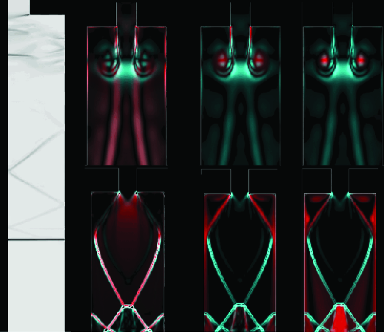
(a) Time-averaged normalized correlation coefficients between disturbance energy flux field and dilatation, vorticity and entropy fields for the inviscid (circles) and viscous (squares) calculations. Inviscid calculations: spatial overlap (white) between flux (cyan) and dilatation, vorticity and entropy (red) for cases (b) $M_i=1.1$
,
$M_i=1.1$
, $\alpha=0.25$
, (c)
$\alpha=0.25$
, (c) $M_i=2.1$
,
$M_i=2.1$
, $\alpha=0.25$
, and (d)
$\alpha=0.25$
, and (d) $M_i=3.5$
,
$M_i=3.5$
, $\alpha=0.25$
.
$\alpha=0.25$
.

This subsubsection further considers the flux of energy disturbances in these different regimes. As might be expected, disturbance energy characteristics are correlated with prominent flow features, such as propagating shocks or convecting eddies. First, consider regime 1, detailed in figure 3. In this case, the disturbance energy flux in the near-field zone is associated with the pair of eddies at the far end of the resulting fluid jet, as shown by figure 8. If the fluid entering the jet is sonic or supersonic, then the dominant sources of disturbance energy flux are either the recirculation zones outside the fluid jet or the oblique shocks/expansion fans within the jet itself. The former appear to dominate in regions where the exiting fluid is either over-expanded (i.e. the pressure of the exiting jet is less than ambient, producing regime 2 in figure 8) or only slightly under-expanded, in which case the jet expands slightly before contracting repeatedly, forming a shock-diamond pattern (regime 3 in figure 8). In cases where the jet is sufficiently under-expanded that the resulting jet fills the channel and does not contract, the oblique shocks/expansion fans are coincident with locations of strongest flux (regime 4 in figure 8). Moreover, there appear to be few or no near-field phenomena of particular note for the converging duct cases (regime 5 in figure 8).
Figure 10 shows the spatial overlap between the disturbance energy flux field and dilatation, vorticity and entropy fields for the inviscid cases. In most cases, the disturbance energy flux field correlates most strongly with the dilatation field, and correlates weakly with the vorticity and entropy fields. As an example, consider the case shown in figure 10(b), where elevated energy flux is correlated most strongly with regions of vortex roll-up. One can clearly observe, however, that of the three fields, the dilatational field corresponds most strongly with the disturbance energy flux. These results indicate that most disturbance energy lies in the dilatational mode. The reasons for this can be understood from the leading-order energy flux term $F_1 \equiv \boldsymbol{\nabla} \boldsymbol{\cdot} (p_1{\boldsymbol {u}}_1)$
. The first-order pressure fluctuation
$F_1 \equiv \boldsymbol{\nabla} \boldsymbol{\cdot} (p_1{\boldsymbol {u}}_1)$
. The first-order pressure fluctuation $p_1$
only has a dilatational component (Lieuwen Reference Lieuwen2012); thus at first order, the disturbance energy flux results from the dilatational mode only. Therefore, any disturbance energy flux from the vortical or entropic disturbances would have to result from higher-order effects whose magnitude is dominated by this first-order effect.
$p_1$
only has a dilatational component (Lieuwen Reference Lieuwen2012); thus at first order, the disturbance energy flux results from the dilatational mode only. Therefore, any disturbance energy flux from the vortical or entropic disturbances would have to result from higher-order effects whose magnitude is dominated by this first-order effect.
For $\alpha<1$
, this trend weakens as the jet becomes less expanded – i.e. as both
$\alpha<1$
, this trend weakens as the jet becomes less expanded – i.e. as both $\alpha$
and
$\alpha$
and $M_i$
increase such that the jet pattern shifts from regime 2 to regime 4. The reason for this can be seen in figure 10(c): for flow regimes 2–4, dilatation values peak in the oblique wave train, whereas the disturbance energy flux reaches local extrema in both the oblique waves and in the surrounding flow separation zone. As the jet pattern shifts to regime 4, the greatest disturbance energy flux values are found in the oblique shocks; however, the disturbance energy reaches local maxima joined to local minima, whereas the dilatation field reaches local minima only. This is why, as shown in figure 10(a), the flux field becomes more negatively correlated with the dilatation field for increasing
$M_i$
increase such that the jet pattern shifts from regime 2 to regime 4. The reason for this can be seen in figure 10(c): for flow regimes 2–4, dilatation values peak in the oblique wave train, whereas the disturbance energy flux reaches local extrema in both the oblique waves and in the surrounding flow separation zone. As the jet pattern shifts to regime 4, the greatest disturbance energy flux values are found in the oblique shocks; however, the disturbance energy reaches local maxima joined to local minima, whereas the dilatation field reaches local minima only. This is why, as shown in figure 10(a), the flux field becomes more negatively correlated with the dilatation field for increasing $\alpha$
for the
$\alpha$
for the $M_i=2.5$
and 3.5 cases. Visually inspecting figure 10(b), the disturbance energy extrema corresponding to the recirculation zones coincide most strongly with those of the vorticity field and, to a lesser extent, the entropy field. Combining these observations, for cases where the area change leads to choked flow, the dilatation field (strongest in the oblique wave train), vorticity field (strongest at the edges of the jet, where shear layers exist) and entropy field (strongest in the area surrounding the jet) are dominant in different spatial structures that rank differently in disturbance energy strength depending on
$M_i=2.5$
and 3.5 cases. Visually inspecting figure 10(b), the disturbance energy extrema corresponding to the recirculation zones coincide most strongly with those of the vorticity field and, to a lesser extent, the entropy field. Combining these observations, for cases where the area change leads to choked flow, the dilatation field (strongest in the oblique wave train), vorticity field (strongest at the edges of the jet, where shear layers exist) and entropy field (strongest in the area surrounding the jet) are dominant in different spatial structures that rank differently in disturbance energy strength depending on $M_i$
and
$M_i$
and $\alpha$
.
$\alpha$
.
The time-averaged, normalized correlation coefficient (defined by (2.27)) is compared between the viscous and inviscid calculations in figure 10(a), showing very clear similarities. The exception appears to be that in the viscous case, the disturbance energy flux becomes increasingly correlated with the entropy mode for converging ducts. This implies that entropy disturbances are more pronounced in the viscous case, and contribute to a greater portion of the disturbance energy.
Relative magnitudes and spatial structures of the dominant disturbance energy accumulation terms for (a) regime 1, (b) regime 2, (c) regime 3, and (d) regime 4. The terms shown in the red, green and blue channels are indicated by the colour triangles in the rightmost column.

Further insight into the disturbance energy flux distribution can be gained by quantifying the terms in the disturbance energy decomposition laid out in (2.37)–(2.42). As discussed in § 2.3.1, this was performed only for the inviscid calculations. For the diverging ducts, this information is summarized in figure 11. The bar graphs detail the relative magnitudes of the time- and space-averaged disturbance energy accumulation terms. The contours showcase the spatial distribution of the three accumulation terms of greatest interest. Taken together, these elucidate the relative importance of various disturbance energy accumulation terms (acoustic/dilatational, vortical, acoustic-vortical, etc.) and the flow structures with which they are correlated. For the case of a weak shock (i.e. regime 1 discussed in the previous paragraphs), acoustic disturbances are responsible for the bulk of the disturbance energy accumulation, with the other fields contributing little to none. This agrees with the information in figure 10(a), in which the disturbance energy flux was most correlated with the dilatation field. Similarly, comparing the RGB contour of figure 11(a) with contours of figure 10(b), the various accumulation terms coincide spatially with their respective fields (i.e. the acoustic accumulation, the red channel of figure 11(a), aligns with the dilatation field; the same holds for the vorticity and entropy fields).
As the incident shock increases in strength, we reach the ‘regime 2’ under-expanded jet of figure 11(b), at which point $\dot {E}_{\Lambda }$
(acoustic disturbance energy accumulation),
$\dot {E}_{\Lambda }$
(acoustic disturbance energy accumulation), $\dot {E}_{\Omega }$
(vortical accumulation) and
$\dot {E}_{\Omega }$
(vortical accumulation) and $\dot {E}_{\Lambda ,\Omega }$
(acoustic-vortical accumulation) have similar magnitudes (although the acoustic is approximately double the other two) and are the dominant contributors to the accumulation. As the incident shock strengthens and the resulting jet becomes more expanded (i.e. the ‘regime 3’ jet of figure 11
c), the latter two terms overwhelm the acoustic accumulation and become the dominant contributors. This shows that the disturbance energy accumulation is dominated by acoustic-vortical products. Additionally, the other four terms (
$\dot {E}_{\Lambda ,\Omega }$
(acoustic-vortical accumulation) have similar magnitudes (although the acoustic is approximately double the other two) and are the dominant contributors to the accumulation. As the incident shock strengthens and the resulting jet becomes more expanded (i.e. the ‘regime 3’ jet of figure 11
c), the latter two terms overwhelm the acoustic accumulation and become the dominant contributors. This shows that the disturbance energy accumulation is dominated by acoustic-vortical products. Additionally, the other four terms ( $\dot {E}_{s}$
,
$\dot {E}_{s}$
, $\dot {E}_{\Lambda , s}$
,
$\dot {E}_{\Lambda , s}$
, $\dot {E}_{\Omega , s}$
and
$\dot {E}_{\Omega , s}$
and $\dot {E}_{\Lambda , \Omega , s}$
) become increasingly important until, in the fully-expanded case of figure 11(d), disturbance energy accumulation is deposited approximately equally between the seven terms. This would appear to result from the emerging entropic mode seen in figure 11(c), reflecting the growing strength of entropy disturbances and, consequently, the growing magnitude of modal cross-products with entropy (i.e.
$\dot {E}_{\Lambda , \Omega , s}$
) become increasingly important until, in the fully-expanded case of figure 11(d), disturbance energy accumulation is deposited approximately equally between the seven terms. This would appear to result from the emerging entropic mode seen in figure 11(c), reflecting the growing strength of entropy disturbances and, consequently, the growing magnitude of modal cross-products with entropy (i.e. $\dot {E}_{\Lambda , s}$
,
$\dot {E}_{\Lambda , s}$
, $\dot {E}_{\Omega , s}$
and
$\dot {E}_{\Omega , s}$
and $\dot {E}_{\Lambda , \Omega , s}$
) in the overall accumulation. This result explains the decreased correlation of the disturbance energy flux with
$\dot {E}_{\Lambda , \Omega , s}$
) in the overall accumulation. This result explains the decreased correlation of the disturbance energy flux with $\Lambda$
,
$\Lambda$
, $\Omega$
and
$\Omega$
and $s$
shown in figure 10 with increased incident shock strength increases; i.e. the energy flux is increasingly dominated by products of these canonical disturbances.
$s$
shown in figure 10 with increased incident shock strength increases; i.e. the energy flux is increasingly dominated by products of these canonical disturbances.
Examining the RGB contours of figures 11(b)and 11(d), acoustic energy accumulation is strongest at the oblique shocks within the supersonic jet, while vortical accumulation is strongest at the edges of the jet, where recirculation zones exist. Examining the entropic accumulation (blue channel) of figure 11(d), the entropic accumulation is also maximized on the jet edges, and has large values between shock diamonds. This last case agrees with figure 10(c); i.e. the acoustic, vortical and entropic accumulations once again appear to coincide with their respective fields, as expected. The acoustic-vortical accumulation ( $\dot {E}_{\Lambda , \Omega }$
), the other dominant contributor for the supersonic jets, is maximized in the Mach disks that separate successive shock diamonds, where the flow is simultaneously expanded and turned. These results suggest that these processes within the jet increase the amount of acoustic-vortical disturbance energy accumulation as the jet expands.
$\dot {E}_{\Lambda , \Omega }$
), the other dominant contributor for the supersonic jets, is maximized in the Mach disks that separate successive shock diamonds, where the flow is simultaneously expanded and turned. These results suggest that these processes within the jet increase the amount of acoustic-vortical disturbance energy accumulation as the jet expands.
Relative magnitudes and spatial structures of the dominant disturbance energy accumulation terms for contracting ducts for three different incident shock strengths. The terms shown in the red, green and blue channels are indicated by the colour triangles in the rightmost column.

For contracting ducts, the distribution of disturbance energy accumulation is summarized in figure 12. Even for weak incident shocks, the acoustic energy accumulation is always smaller than the acoustic-vortical accumulation. The former appears to be strongest at the transverse shocks that persist shortly after transmission into the smaller duct, while the latter appears to dominate in the interior of these shocks. Thus for contracting ducts, the acoustic-vortical accumulation is a significant contributor to the overall disturbance energy. Also present is the acoustic-entropic accumulation, which appears to be strongest near the duct boundaries. As the incident shock is strengthened, the entropic and acoustic-entropic accumulations outweigh the acoustic-vortical accumulation, while the acoustic accumulation maintains its relative importance. This may explain why the correlation between the disturbance energy flux and dilatation fields remains constant with increasing shock strength, as shown in figure 10(a). Combined with the diminishing importance of the vortical accumulation, these observations suggest that vortical disturbances become overwhelmed by entropic ones as incident shock strength increases; these entropic disturbances, in conjunction with strong pressure gradients (acoustic disturbances), produce strong acoustic-entropic disturbance energy.
Combining the above observations, the differing jet patterns in the near-field zones have varying strengths in each of the seven disturbance energy accumulation terms. Acoustic disturbances are strong for all jet patterns observed; as the incident shock increases in strength and produces stronger jets, these disturbances work in tandem with emerging vortical and entropic disturbances to produce cross-product disturbance energy accumulation. Energy accumulation is dominated by acoustic and vortical disturbance products for contracting ducts; the bar graph of figure 12(b) suggests that even relatively weak vortical disturbances are responsible for a significant portion of the energy accumulation when acoustic disturbances are present. Furthermore, these decompositions provide further insight into the alternative visualization approach of determining the correlation of instantaneous disturbance energy flux with the dilatation, vorticity and entropy fields.
3.2. Shock reflections and transmission results
Dependence of reflection and transmission coefficients upon area ratio. Viscous and inviscid results are denoted by circles and squares, respectively.

Figure 13 plots the dependence of the shock pressure reflection and transmission coefficients, $R$
and
$R$
and $T$
, on area ratio at different incident Mach numbers, showing both the quasi-1-D and inviscid/viscous CFD calculations. The right-hand plot shows the difference between the two calculation approaches. Interestingly, the transmission coefficient is much less sensitive to the incident shock strength than the reflection coefficient. As expected,
$T$
, on area ratio at different incident Mach numbers, showing both the quasi-1-D and inviscid/viscous CFD calculations. The right-hand plot shows the difference between the two calculation approaches. Interestingly, the transmission coefficient is much less sensitive to the incident shock strength than the reflection coefficient. As expected, $T$
is less than 1 for area divergences (
$T$
is less than 1 for area divergences ( $\alpha \lt\, 1$
) and greater than 1 for area convergences. The reflection coefficient varies strongly with both
$\alpha \lt\, 1$
) and greater than 1 for area convergences. The reflection coefficient varies strongly with both $\alpha$
and
$\alpha$
and $M_i$
. For a large enough area ratio (i.e. a sudden enough contraction), the reflection coefficient increases in a nearly linear manner with
$M_i$
. For a large enough area ratio (i.e. a sudden enough contraction), the reflection coefficient increases in a nearly linear manner with $M_i$
; this represents a limiting behaviour for the reflection coefficient.
$M_i$
; this represents a limiting behaviour for the reflection coefficient.
As might be expected, discrepancies between the quasi-1-D and computed results grow as the area ratio deviates from unity in either direction (noting that the exact solution is 1-D when the area ratio is unity). Overall, however, the quasi-1-D calculations predict reasonably accurate values of $R$
and
$R$
and $T$
. This overall good agreement suggests that while 2-D disturbances have pronounced effects on the flow field close to the area jump, their lasting effects on the transmitted and reflected waves are fairly minor. This result is not only fundamentally interesting but also consequential for reduced-order models of the phenomenon, as it shows that quasi-1-D considerations can be used to quite accurately understand and quantify the effect of the area change on the reflected and transmitted shock waves.
$T$
. This overall good agreement suggests that while 2-D disturbances have pronounced effects on the flow field close to the area jump, their lasting effects on the transmitted and reflected waves are fairly minor. This result is not only fundamentally interesting but also consequential for reduced-order models of the phenomenon, as it shows that quasi-1-D considerations can be used to quite accurately understand and quantify the effect of the area change on the reflected and transmitted shock waves.
Comparing the viscous and inviscid calculations, there is quite close quantitative agreement, with both $R$
and
$R$
and $T$
being generally lower in the viscous case. These differences remain small but grow with increasing
$T$
being generally lower in the viscous case. These differences remain small but grow with increasing $M_i$
, but not necessarily with increasing
$M_i$
, but not necessarily with increasing $\alpha$
. As noted in the previous subsection, the nature of the near-field behaviour is altered by the presence of viscosity. Furthermore, the presence of viscous boundary layers and possibly other 2-D phenomena behind the transmitted and reflected waves (particularly behind the reflected shocks in the converging duct cases, as discussed in the previous subsection) does not lead to significant deviation. The calculation of these coefficients involves identifying flow variables in uniform regions around these waves (see figure 2 and (2.14)–(2.15)). When these regions are no longer uniform, it becomes increasingly difficult to assign a single variable to these regions, so it should be emphasized that there is no longer a one-to-one correspondence between the three cases (quasi-1-D, 2-D inviscid and 2-D viscous).
$\alpha$
. As noted in the previous subsection, the nature of the near-field behaviour is altered by the presence of viscosity. Furthermore, the presence of viscous boundary layers and possibly other 2-D phenomena behind the transmitted and reflected waves (particularly behind the reflected shocks in the converging duct cases, as discussed in the previous subsection) does not lead to significant deviation. The calculation of these coefficients involves identifying flow variables in uniform regions around these waves (see figure 2 and (2.14)–(2.15)). When these regions are no longer uniform, it becomes increasingly difficult to assign a single variable to these regions, so it should be emphasized that there is no longer a one-to-one correspondence between the three cases (quasi-1-D, 2-D inviscid and 2-D viscous).
Power reflection, transmission and accumulation coefficients over the cases studied. Viscous and inviscid results are denoted by circles and squares, respectively.

We next consider power reflection, transmission and accumulation. We start this discussion by noting that these results are strongly influenced by the transient and frontal nature of the shocks; i.e. the post-shock state persists indefinitely, and does not return to its condition before the shock arrived. As such, the results are less physically intuitive than the case of, say, a shock ‘pulse’, in which the fluid behind the shock eventually returns to rest (when, for example, a piston compresses the gas for a certain time before returning to rest). Moreover, the transient nature of the problem implies that the energy fluxes into and out of the domain need not balance, as energy can accumulate.
The dependence of $R_\Pi$
,
$R_\Pi$
, $T_\Pi$
and
$T_\Pi$
and $C_e$
upon area ratio, computed for both flow models, is shown in figure 14. The deviation between the quasi-1-D and CFD results is again plotted on the right. Once again, the values are quite similar between the two models. Moreover, as with
$C_e$
upon area ratio, computed for both flow models, is shown in figure 14. The deviation between the quasi-1-D and CFD results is again plotted on the right. Once again, the values are quite similar between the two models. Moreover, as with $T$
,
$T$
, $T_\Pi$
and
$T_\Pi$
and $C_e$
, the largest deviations appear for larger area changes. Unlike
$C_e$
, the largest deviations appear for larger area changes. Unlike $T$
, however,
$T$
, however, $T_\Pi$
varies with both
$T_\Pi$
varies with both $M_i$
and
$M_i$
and $\alpha$
. Furthermore,
$\alpha$
. Furthermore, $R_I$
shows little variation between the two results except in the case of very strong and very weak shocks interacting with a large area divergence; this contrasts with the behaviour of
$R_I$
shows little variation between the two results except in the case of very strong and very weak shocks interacting with a large area divergence; this contrasts with the behaviour of $R$
noted in the previous subsection.
$R$
noted in the previous subsection.
Unlike $T$
,
$T$
, $T_{\Pi }$
exceeds unity for sufficiently strong shocks for diverging ducts with certain area ratios. This does not indicate that energy conservation is violated; it merely indicates the presence of stronger energy accumulation terms in the region between the shocks owing to the transient nature of the problem (see (2.25) and (2.26)). For instance, consider the balance of total energy between the waves in the weak shock case. By employing the perturbation methods discussed in the next subsection, the following can be demonstrated for the quasi-1-D method:
$T_{\Pi }$
exceeds unity for sufficiently strong shocks for diverging ducts with certain area ratios. This does not indicate that energy conservation is violated; it merely indicates the presence of stronger energy accumulation terms in the region between the shocks owing to the transient nature of the problem (see (2.25) and (2.26)). For instance, consider the balance of total energy between the waves in the weak shock case. By employing the perturbation methods discussed in the next subsection, the following can be demonstrated for the quasi-1-D method:
 \begin{equation} \frac {\mbox {transmitted total power}}{\mbox {incident total power}} = \frac {\rho _4u_4h_{T4}A_t}{\rho _3u_3h_{T3}A_i} = \frac {2}{\alpha + 1} + \mathcal {O}(M_i-1), \end{equation}
 \begin{equation} \frac {\mbox {reflected total power}}{\mbox {incident total power}} = \frac {\rho _3u_3h_{T3} - \rho _7u_7h_{T7}}{\rho _3u_3h_{T3}} = \frac {\alpha - 1}{\alpha + 1} + \mathcal {O}(M_i-1), \end{equation}
 \begin{equation} \frac {\mbox {incident}-\mbox{transmitted}-\mbox{reflected total power}}{\mbox {incident total power}} \propto (\alpha - 1)(M_i - 1)^5 + \mathcal {O}(M_i - 1)^6. \end{equation}
One notes the following from the above expressions. First, even in the acoustic ( $M_i=1$
) limit, the total power transmission ratio exceeds unity, but this is balanced by a negative total power reflection coefficient, such that the two sum to unity up to
$M_i=1$
) limit, the total power transmission ratio exceeds unity, but this is balanced by a negative total power reflection coefficient, such that the two sum to unity up to $\mathcal {O}(M_i - 1)$
. This unfamiliar result pertains to the total energy, not the disturbance energy; the latter produces the more familiar result for linear acoustics, as discussed in Appendix B. This is made possible by the transient nature of the physics. That is, the time derivative in the energy equation permits an imbalance in the fluxes that can be positive or negative. Second, the third expression indicates that at
$\mathcal {O}(M_i - 1)$
. This unfamiliar result pertains to the total energy, not the disturbance energy; the latter produces the more familiar result for linear acoustics, as discussed in Appendix B. This is made possible by the transient nature of the physics. That is, the time derivative in the energy equation permits an imbalance in the fluxes that can be positive or negative. Second, the third expression indicates that at $\mathcal {O}(M_i - 1)$
, the power of the transmitted and reflected waves exceeds that of the incident wave for diverging ducts (since
$\mathcal {O}(M_i - 1)$
, the power of the transmitted and reflected waves exceeds that of the incident wave for diverging ducts (since $\alpha-1<0$
). This result is due to the contact surface present in the quasi-1-D model. Such flow disturbances (the reflected wave and contact surface in this example) supply the necessary power to allow the transmitted power to exceed that of the incident shock.
$\alpha-1<0$
). This result is due to the contact surface present in the quasi-1-D model. Such flow disturbances (the reflected wave and contact surface in this example) supply the necessary power to allow the transmitted power to exceed that of the incident shock.
In nearly every case except those for weak shocks, $C_e$
is over-predicted by the quasi-1-D theory. Thus despite not explicitly accounting for 2-D near-field disturbances, the quasi-1-D theory partially captures the disturbance energy accumulation (the secondary transmitted shock of zone Ic in figure 1, for instance, is one phenomenon responsible for this) not seen in the 2-D results.
$C_e$
is over-predicted by the quasi-1-D theory. Thus despite not explicitly accounting for 2-D near-field disturbances, the quasi-1-D theory partially captures the disturbance energy accumulation (the secondary transmitted shock of zone Ic in figure 1, for instance, is one phenomenon responsible for this) not seen in the 2-D results.
These quasi-1-D calculations can be generalized by adding additional physics to partially capture 2-D effects. For example, consider the recirculation patterns exhibited for weak shock interactions with a diverging duct (behaviour (1) in figure 8). This flow separation associated with a sudden flow expansion causes the flow to increase in entropy. Flow separation can be incorporated into the quasi-1-D approach by accounting for this entropy jump. Using the entropy jump value developed previously by Isaacson (Reference Isaacson2011), valid for $\alpha \in(0.2, 1)$
, leads to
$\alpha \in(0.2, 1)$
, leads to
 \begin{equation} \Delta s = \mathscr {C}_v[(1 - \alpha )^2 + (1 - \alpha )^6]\gamma \delta M_7^2. \end{equation}
Here, $\mathscr {C}_v$
is the constant volume specific heat. This can be combined with the steady energy conservation equation and the Gibbs relations to obtain a more accurate set of relations between the pre- and post-area change conditions. The effects of such a correction can be most clearly seen in
$\mathscr {C}_v$
is the constant volume specific heat. This can be combined with the steady energy conservation equation and the Gibbs relations to obtain a more accurate set of relations between the pre- and post-area change conditions. The effects of such a correction can be most clearly seen in $R_\Pi$
, as shown in figure 15; for the most severe area increase studied, errors between quasi-1-D and CFD were reduced from 56 % to 3 % for the inviscid calculations.
$R_\Pi$
, as shown in figure 15; for the most severe area increase studied, errors between quasi-1-D and CFD were reduced from 56 % to 3 % for the inviscid calculations.
Power reflection coefficient for various diverging ducts calculated using the quasi-1-D method, the corrected quasi-1-D method accounting for flow separation, and 2-D inviscid CFD.

3.3. Analytical results for weak shocks
The results of the previous subsection can be further interpreted by writing explicit solutions from the quasi-1-D theory, obtained by a perturbation expansion in powers of $(M_i - 1)$
. We now present results with the leading-order nonlinear corrections for
$(M_i - 1)$
. We now present results with the leading-order nonlinear corrections for $T$
,
$T$
, $R$
,
$R$
, $T_{\Pi }$
,
$T_{\Pi }$
, $R_{\Pi }$
and
$R_{\Pi }$
and $C_e$
from their linear acoustic relations (see Appendix A for details):
$C_e$
from their linear acoustic relations (see Appendix A for details):
 \begin{align} T &= \frac {2 \alpha }{\alpha + 1} + \frac {2\alpha (\alpha - 1)(\delta - 1)}{\kappa (\alpha + 1)^2}\,(M_i - 1) + \mathcal {O}(M_i - 1)^2, \end{align}
 \begin{align} R &= \frac {\alpha - 1}{\alpha + 1} + \frac {2(\alpha - 1)(\alpha \kappa + 2)}{\kappa (\alpha + 1)^2}\,(M_i - 1) + \mathcal {O}(M_i - 1)^2, \end{align}
 \begin{align} T_{\Pi } &= \frac {4 \alpha }{(\alpha + 1)^2} + \frac {4\alpha (\alpha - 1)(\delta - 1)}{\kappa (\alpha + 1)^3}\,(M_i - 1) + \mathcal {O}(M_i - 1)^2, \end{align}
 \begin{align} R_{\Pi } &= \left (\frac {\alpha - 1}{\alpha + 1}\right )^2 - \frac {4\alpha (\alpha - 1)(\delta - 1)}{\kappa (\alpha + 1)^3}\,(M_i - 1) + \mathcal {O}(M_i - 1)^2, \end{align}
 \begin{align} C_e &= \left \{ \begin{array}{ l l } \dfrac {64\delta (\alpha - 1)\alpha ^2(1 + \alpha [4 + 7\alpha ])}{3\kappa ^3(\alpha + 1)^6}\,(M_i - 1)^4 + \mathcal {O}(M_i - 1)^5, & \alpha \lt 1, \\ \dfrac {128\delta (\alpha - 1)\alpha ^3}{\kappa ^3(\alpha + 1)^5}\,(M_i - 1)^4 + \mathcal {O}(M_i - 1)^5, & \alpha \gt 1. \end{array} \right . \end{align}
Several important observations can be made from these equations. First, all of the expressions limit to their classical acoustic expressions (see Kinsler et al. Reference Kinsler, Frey, Coppens and Sanders2000). While the above terms depend only on $\alpha$
in the acoustic limit, nonlinear corrections depend on the incident shock strength and the specific heat ratio of the gas,
$\alpha$
in the acoustic limit, nonlinear corrections depend on the incident shock strength and the specific heat ratio of the gas, $\gamma$
. Second, while nonlinear corrections to
$\gamma$
. Second, while nonlinear corrections to $T$
,
$T$
, $R$
,
$R$
, $T_{\Pi }$
,
$T_{\Pi }$
, $R_{\Pi }$
, occur at leading order in
$R_{\Pi }$
, occur at leading order in $(M_i - 1)$
, the correction to
$(M_i - 1)$
, the correction to $C_e$
occurs at
$C_e$
occurs at $\mathcal{O}(M_i-1)^4$
, implying that it is very weak at low Mach numbers. Since the quasi-1-D theory accounts for only dilatational and entropy disturbances (i.e. not vortical), energy exchange occurs only between these two disturbances in the quasi-1-D problem. Moreover, since at
$\mathcal{O}(M_i-1)^4$
, implying that it is very weak at low Mach numbers. Since the quasi-1-D theory accounts for only dilatational and entropy disturbances (i.e. not vortical), energy exchange occurs only between these two disturbances in the quasi-1-D problem. Moreover, since at $\mathcal {O}(M_i-1)^2$
and lower there is no entropy produced by shocks, energy in the dilatational disturbances is conserved to that order. The area change rearranges the energy in the incident shock between the reflected and transmitted shock, but the power carried away by these reflected/transmitted waves exactly equals that of the incident wave up to
$\mathcal {O}(M_i-1)^2$
and lower there is no entropy produced by shocks, energy in the dilatational disturbances is conserved to that order. The area change rearranges the energy in the incident shock between the reflected and transmitted shock, but the power carried away by these reflected/transmitted waves exactly equals that of the incident wave up to $\mathcal {O}(M_i-1)^3$
. To further understand this point for this specific problem, consider (2.26). In this case, the area change is isentropic and steady, so it has no net disturbance energy flux, leaving only the unsteady accumulation in the near-field zone, given by (2.24). The leading-order contribution to the power accumulation is the jump in stagnation enthalpy flux across the contact surface. Because the pressure and velocity are continuous across the contact surface, this reduces to
$\mathcal {O}(M_i-1)^3$
. To further understand this point for this specific problem, consider (2.26). In this case, the area change is isentropic and steady, so it has no net disturbance energy flux, leaving only the unsteady accumulation in the near-field zone, given by (2.24). The leading-order contribution to the power accumulation is the jump in stagnation enthalpy flux across the contact surface. Because the pressure and velocity are continuous across the contact surface, this reduces to
 \begin{equation} \rho _4u_4h_{T4} - \rho _5u_5h_{T5} = \frac {u_4^3}{2}\,(\rho _4 - \rho _5). \end{equation}
This expression explicitly shows that $u_4^3$
is
$u_4^3$
is $\mathcal {O}(M_i-1)^3$
in magnitude. Since the contact surface exists only at
$\mathcal {O}(M_i-1)^3$
in magnitude. Since the contact surface exists only at $\mathcal {O}(M_i-1)^3$
and higher, the jump in density across the contact surface is
$\mathcal {O}(M_i-1)^3$
and higher, the jump in density across the contact surface is $\mathcal {O}(M_i-1)^3$
in magnitude; thus the unsteady accumulation of disturbance energy in the near-field zone is only
$\mathcal {O}(M_i-1)^3$
in magnitude; thus the unsteady accumulation of disturbance energy in the near-field zone is only $\mathcal {O}(M_i - 1)^6$
in magnitude. Because
$\mathcal {O}(M_i - 1)^6$
in magnitude. Because $I_i$
is
$I_i$
is $\mathcal {O}(M_i - 1)^2$
in magnitude,
$\mathcal {O}(M_i - 1)^2$
in magnitude, $C_e$
is
$C_e$
is $\mathcal {O}(M_i - 1)^4$
in magnitude. Summarizing the above points, the quasi-1-D theory accounts for only entropy and acoustic disturbances; thus there is disturbance energy accumulation up to the order at which entropy disturbances appear. Consequently, transfer of energy out of the shock into other disturbances occurs only at very high order (i.e. its magnitude is quite small). This result was noted more generally by Jenvey (Reference Jenvey1989), who stated that acoustic energy transport due to mass flux fluctuations is conserved to arbitrary order for irrotational, homentropic flow, and by Doak (Reference Doak1989), who noted that such flows exist in a ‘local fluctuating dynamical equilibrium’ in which the net power flux is zero.
$\mathcal {O}(M_i - 1)^4$
in magnitude. Summarizing the above points, the quasi-1-D theory accounts for only entropy and acoustic disturbances; thus there is disturbance energy accumulation up to the order at which entropy disturbances appear. Consequently, transfer of energy out of the shock into other disturbances occurs only at very high order (i.e. its magnitude is quite small). This result was noted more generally by Jenvey (Reference Jenvey1989), who stated that acoustic energy transport due to mass flux fluctuations is conserved to arbitrary order for irrotational, homentropic flow, and by Doak (Reference Doak1989), who noted that such flows exist in a ‘local fluctuating dynamical equilibrium’ in which the net power flux is zero.
These quasi-1-D near-field power accumulation results can be similarly modified to account for flow separation using the correction developed in (3.4). If this equation is added to the system to be solved, then one obtains the following new expressions for the above variables:
 \begin{align} T &= \frac {2 \alpha }{\alpha + 1} + \left [\frac {2\alpha (\alpha - 1)(\delta - 1)}{\kappa (\alpha + 1)^2} - \frac {4\alpha\, F(\alpha )}{\kappa (1 + \alpha )^3}\right ](M_i - 1) + \mathcal {O}(M_i - 1)^2, \end{align}
 \begin{align} R &= \frac {\alpha - 1}{\alpha + 1} + \left [\frac {2(\alpha - 1)(\alpha \kappa + 2)}{\kappa (\alpha + 1)^2} + \frac {4\,F(\alpha )}{\kappa (1 + \alpha )^3}\right ](M_i - 1) + \mathcal {O}(M_i - 1)^2, \end{align}
 \begin{align} T_{\Pi } &= \frac {4 \alpha }{(\alpha + 1)^2} + 4\alpha \left [\frac {(\alpha - 1)(\delta - 1)}{\kappa (\alpha + 1)^3} - \frac {4\,F(\alpha )}{\kappa (1 + \alpha )^3} \right ](M_i - 1) + \mathcal {O}(M_i - 1)^2, \end{align}
 \begin{align} R_{\Pi } &= \left (\frac {\alpha - 1}{\alpha + 1}\right )^2 - 4\alpha (\alpha - 1)\left [\frac {\delta - 1}{\kappa (\alpha + 1)^3} - \frac {2\,F(\alpha )}{\kappa (\alpha + 1)^4}\right ](M_i - 1) + \mathcal {O}(M_i - 1)^2, \end{align}
 \begin{align} C_e &= \frac {8\,F(\alpha )}{\kappa (1 + \alpha )^3}(M_i - 1) + \mathcal {O}(M_i - 1)^2 , \end{align}
where $F(\alpha ) \equiv (1 - \alpha )^2 + (1 - \alpha )^6$
. This equation has noteworthy consequences. First, the accumulation coefficient is now
$F(\alpha ) \equiv (1 - \alpha )^2 + (1 - \alpha )^6$
. This equation has noteworthy consequences. First, the accumulation coefficient is now $\mathcal {O}(M_i - 1)$
in magnitude. Thus although this coefficient is small in both cases, Rudinger’s method under-predicts the accumulation by orders of magnitude in the weak shock case (in the framework of (3.4)). Second, the aforementioned discrepancies in
$\mathcal {O}(M_i - 1)$
in magnitude. Thus although this coefficient is small in both cases, Rudinger’s method under-predicts the accumulation by orders of magnitude in the weak shock case (in the framework of (3.4)). Second, the aforementioned discrepancies in $T$
,
$T$
, $R$
,
$R$
, $T_{\Pi }$
and
$T_{\Pi }$
and $R_{\Pi }$
are first-order effects. It is also worth noting that using (3.4) correctly predicts the sign of this discrepancy; neglecting these effects causes one to over-predict
$R_{\Pi }$
are first-order effects. It is also worth noting that using (3.4) correctly predicts the sign of this discrepancy; neglecting these effects causes one to over-predict $T$
,
$T$
, $T_{\Pi }$
and
$T_{\Pi }$
and $R_{\Pi }$
, and under-predict
$R_{\Pi }$
, and under-predict $R$
. Furthermore, because of the form of
$R$
. Furthermore, because of the form of $F(\alpha )$
, these effects are most significant at lower
$F(\alpha )$
, these effects are most significant at lower $\alpha$
(i.e. more severe area increases), but their prominence diminishes sharply with increasing
$\alpha$
(i.e. more severe area increases), but their prominence diminishes sharply with increasing $\alpha$
(i.e. for less severe area increases).
$\alpha$
(i.e. for less severe area increases).
4. Conclusions
The interactions between shock waves and discrete area changes have been studied using both computational and analytical approaches. This was done to both generalize existing results and further understand how energy moves between dilatational, vortical and entropic disturbances in shock wave interactions with complex geometries. The computational approach reveals five categories of 2-D transient ‘near-field’ phenomena that persist near the area change after the passage of the incident shock; these categories, which depend on 2-D flow features, are distinct from those used in the quasi-1-D theory, which depend on the structure of the 1-D wave patterns (contact surfaces, reflected shocks or expansion waves, transmitted shocks). The observed flow regime depends on the incident shock strength and the area ratio. The transfer of disturbance energy from the shock waves to such near-field disturbances was also analysed. This revealed that disturbance energy is spatially correlated with flow regimes in the near field (vortex roll-up, shock diamonds, etc.). The flow regime responsible for the greatest disturbance energy flux depends on the incident Mach number and area ratio.
This work represents the first study, to our knowledge, investigating how disturbance energy is produced by and associated with acoustic, vortical and entropic disturbances of arbitrary magnitude during the shock–area change interaction. Correlating the disturbance energy flux with dilatation, vorticity and entropy reveals that the dominant disturbance depends on the category of near-field behaviour. For example, for a weak shock, dilatational disturbances are strongest. Formally decomposing the disturbance energy further reveals the relative importance of these disturbances, and that they interact to produce disturbance energy in nonlinear cross-products. For diverging ducts, such interactions eventually cause disturbance energy to change at nearly equal rates across all disturbances and their cross-products. For both ducts, vortical disturbances contribute less disturbance energy than entropy disturbances with increasing shock strength; these disturbances interact with ever-present acoustic disturbances to produce energy in cross-product terms. This agrees with the asymptotic analysis in the weak shock limit: for stronger incident shocks, entropy disturbances become more prominent and accumulate more energy.
Comparison between CFD and the quasi-1-D method reveals good agreement between the two. This suggests that quasi-1-D methods accurately capture the asymptotic behaviour of wave reflections and transmissions, an important observation considering the vast differences in computational complexity between these methods. However, the near-field power accumulation resulting from the travelling shock waves can be off by orders of magnitude for weak shocks. Furthermore, we show how to resolve some of the aforementioned quantitative differences by accounting for entropy production associated with flow separation in the near field.
These results show that shock transmission is effected primarily by area ratio, while shock reflection is greatly influenced by both area ratio and incident Mach number. For large enough area contractions, the reflection coefficient is influenced by incident Mach number only. Using perturbation methods, we quantified the order of magnitude of important physical effects such as power accumulation, and provide analytic, asymptotic expressions for variables of interest. We demonstrated that accumulation has a notably low order of magnitude in the weak shock case. However, this order of magnitude, while low in both cases, is severely under-predicted when near-field phenomena are neglected. This is because the quasi-1-D method accounts for only dilatational and entropic disturbances; because the latter appear only at high orders, this method conserves dilatational energy in the shocks to third order. This showcases the readiness of physical insight and ease of calculation provided by such methods, improving both the simplicity and transparency of quasi-1-D methods.
Funding.
This research has been partially funded by the US Air Force Office of Scientific Research (contract no. FA9550-23-1-0222, contract monitor Dr C. Li).
Declaration of interests.
The authors report no conflict of interest.
Appendix A. Perturbation expansion for weak shocks
In this appendix, we present asymptotic, quasi-1-D results referred to in § 2.1. In general, one cannot obtain an analytical expression for $R$
and
$R$
and $T$
using Rudinger’s method. However, such expressions can be obtained by expanding the governing equations in powers of
$T$
using Rudinger’s method. However, such expressions can be obtained by expanding the governing equations in powers of $(M_i-1) $
. During this interaction, we have the following system of equations:
$(M_i-1) $
. During this interaction, we have the following system of equations:
 \begin{align} \alpha &= \frac {M_5}{M_7} \left (\frac {1 + \delta M_7^2}{1 + \delta M_5^2} \right )^{{\kappa }/{2\delta }}, \\[-3pt] \nonumber \end{align}
 \begin{align} p_5 &= p_7 \left ( \frac {1 + \delta M_7^2}{1 + \delta M_5^2} \right )^{{\gamma }/{2 \delta }}, \\[-3pt] \nonumber\end{align}
 \begin{align} u_5 &= M_5c_5 = M_5c_7\left (\frac {1 + \delta M_7^2}{1 + \delta M_5^2} \right )^{{1}/{2}}, \\[-3pt] \nonumber\end{align}
 \begin{align} u_5 &= u_4 = \frac {c_1}{\kappa } \left ( \sqrt {\frac {\kappa p_5 + \delta p_1}{\gamma p_1}} - \sqrt {\frac {\gamma p_1}{\kappa p_5 +p \delta p_1}} \right ). \\[-3pt] \nonumber\end{align}
The first equation is obtained by combining the conservation equations for mass and energy with the Poisson adiabat (i.e. (2.1), (2.3) and (2.10)), the second equation simply states that the total pressure is conserved throughout the area discontinuity (consistent with isentropic flow), and the third equation is an alternate expression of the energy conservation equation. The final equation is obtained from the normal shock relations across the transmitted shock after some algebra. The numerical subscripts are summarized in figure 2. The type of reflected wave depends on whether the area increases (resulting in a reflected expansion wave) or decreases (resulting in a reflected shock). For now, we limit consideration to the former case, wherein we have the following equations for $p_7$
and
$p_7$
and $c_7$
:
$c_7$
:
 \begin{equation} p_7 = p_3\left (\frac {1 + \delta M_3}{1 + \delta M_7} \right )^{{\gamma }/{\delta }}, \end{equation}
 \begin{equation} c_7 = c_3\left (\frac {1 + \delta M_3}{1 + \delta M_7} \right ). \end{equation}
This results in a system of four nonlinear equations for the variables $M_5$
,
$M_5$
, $M_7$
,
$M_7$
, $p_5$
and
$p_5$
and $u_5$
. Although this cannot be solved explicitly in general, explicit solutions can be determined to the desired order of accuracy by expanding each variable in the following manner:
$u_5$
. Although this cannot be solved explicitly in general, explicit solutions can be determined to the desired order of accuracy by expanding each variable in the following manner:
 \begin{align} \begin{aligned} M_7 \equiv \nu _0 + \nu _1 + \cdots + \nu _n, \quad M_5 \equiv \mu _0 + \mu _1 + \cdots + \mu _n, \\ \Pi _5 \equiv \frac {p_5}{p_1} - 1 \equiv \pi _0 + \pi _1 + \cdots + \pi _n, \quad u_5 \equiv v_0 + v_1 + \cdots + v_n. \end{aligned} \end{align}
At order $n$
, we have the following system of linear equations for
$n$
, we have the following system of linear equations for $(\nu , \mu , \pi , v)_n$
:
$(\nu , \mu , \pi , v)_n$
:
 \begin{equation} \begin{bmatrix} A_CB_C & A_CC_C & 1 & 0 \\ A_VB_V & A_VC_V & 0 & 1 \\ B_A & C_A & 0 & 0 \\ 0 & 0 & -D_W(2\gamma + \kappa P_n) & 1 \end{bmatrix} \begin{bmatrix} \nu _n \\ \mu _n \\ \pi _n \\ v_n \end{bmatrix} = \begin{bmatrix} A_C - P_n - 1 \\ M_nA_V - V_n \\ A_A \alpha - 1 \\ 2P_nD_W(\gamma + \kappa P_n) - V_n \end{bmatrix}, \end{equation}
 \begin{gather*} N_n \equiv \sum _{k=0}^{n-1} \nu _k, \quad M_n \equiv \sum _{k=0}^{n-1} \mu _k, \quad P_n \equiv \sum _{k=0}^{n-1} \pi _k, \quad V_n \equiv \sum _{k=0}^{n-1}v_k, \\[3pt]
A_C \equiv \frac {p_3}{p_1} \left (\frac {1 + \delta M_3}{1 + \delta N_n} \right )^{{\gamma }/{\delta }} \left (\frac {1 + \delta N_n^2}{1 + \delta M_n^2} \right )^{{\gamma }/{2\delta }}, \\[3pt]
A_V \equiv a_3 \left ( \frac {1 + \delta M_3}{1 + \delta N_n} \right )\left (\frac {1 + \delta N_n^2}{1 + \delta M_n^2} \right )^{{1}/{2}}, \\[3pt]
A_A \equiv \frac {N_n}{M_n} \left (\frac {1 + \delta M_n^2}{1 + \delta N_n^2} \right )^{{\kappa }/{2 \delta }}, \\[3pt]
B_C \equiv \frac {\gamma (1 - N_n)}{(1 + \delta N_n)(1 + \delta N_n^2)}, \quad B_V \equiv \frac {\delta M_n(1 - N_n)}{(1 + \delta N_n)(1 + \delta N_n^2)}, \quad B_A \equiv \frac {N_n^2 - 1}{N_n(1 + \delta N_n^2)}, \\[3pt]
C_C \equiv \frac {\gamma M_n}{1 + \delta M_n^2}, \quad C_V \equiv -\frac {1}{1 + \delta N_n^2}, \quad C_A \equiv \frac {1 - M_n^2}{M_n(1 + \delta M_n^2)}, \\[3pt]
D_W \equiv \frac {c_1}{2\gamma ^2} \left (\frac {\gamma }{\gamma + \kappa P_n} \right )^{{3}/{2}}. \end{gather*}
\begin{gather*} N_n \equiv \sum _{k=0}^{n-1} \nu _k, \quad M_n \equiv \sum _{k=0}^{n-1} \mu _k, \quad P_n \equiv \sum _{k=0}^{n-1} \pi _k, \quad V_n \equiv \sum _{k=0}^{n-1}v_k, \\[3pt]
A_C \equiv \frac {p_3}{p_1} \left (\frac {1 + \delta M_3}{1 + \delta N_n} \right )^{{\gamma }/{\delta }} \left (\frac {1 + \delta N_n^2}{1 + \delta M_n^2} \right )^{{\gamma }/{2\delta }}, \\[3pt]
A_V \equiv a_3 \left ( \frac {1 + \delta M_3}{1 + \delta N_n} \right )\left (\frac {1 + \delta N_n^2}{1 + \delta M_n^2} \right )^{{1}/{2}}, \\[3pt]
A_A \equiv \frac {N_n}{M_n} \left (\frac {1 + \delta M_n^2}{1 + \delta N_n^2} \right )^{{\kappa }/{2 \delta }}, \\[3pt]
B_C \equiv \frac {\gamma (1 - N_n)}{(1 + \delta N_n)(1 + \delta N_n^2)}, \quad B_V \equiv \frac {\delta M_n(1 - N_n)}{(1 + \delta N_n)(1 + \delta N_n^2)}, \quad B_A \equiv \frac {N_n^2 - 1}{N_n(1 + \delta N_n^2)}, \\[3pt]
C_C \equiv \frac {\gamma M_n}{1 + \delta M_n^2}, \quad C_V \equiv -\frac {1}{1 + \delta N_n^2}, \quad C_A \equiv \frac {1 - M_n^2}{M_n(1 + \delta M_n^2)}, \\[3pt]
D_W \equiv \frac {c_1}{2\gamma ^2} \left (\frac {\gamma }{\gamma + \kappa P_n} \right )^{{3}/{2}}. \end{gather*}
Solving for $M_5$
,
$M_5$
, $M_7$
,
$M_7$
, $p_5$
, and
$p_5$
, and $u_5$
closes the system.
$u_5$
closes the system.
One can obtain simplified expressions for certain terms of interest by expanding them in a Taylor series in $M_i$
centred about 1. The first two terms in the expansions for each variable are
$M_i$
centred about 1. The first two terms in the expansions for each variable are $\mathcal{O}(M_i - 1)$
and
$\mathcal{O}(M_i - 1)$
and $\mathcal{O}(M_i - 1)^2$
, respectively, while the third term in each expansion is
$\mathcal{O}(M_i - 1)^2$
, respectively, while the third term in each expansion is $\mathcal{O}(M_i - 1)^3$
. For comparison, consider the entropy jump across the incident shock, given by
$\mathcal{O}(M_i - 1)^3$
. For comparison, consider the entropy jump across the incident shock, given by
 \begin{equation} \begin{aligned} \Delta s &= \mathscr {C}_v\left [\log \left (\frac {p_3}{p_1} \right ) - \gamma \log \left (\frac {\rho _3}{\rho _1} \right )\right ] \\
&= \mathscr {C}_v\left [\log \left (\frac {\gamma M_i^2 -\delta }{\kappa } \right ) - \gamma \log \left (\frac {\kappa M_i^2}{\delta M_i^2 + 1} \right )\right ]. \end{aligned} \end{equation}
\begin{equation} \begin{aligned} \Delta s &= \mathscr {C}_v\left [\log \left (\frac {p_3}{p_1} \right ) - \gamma \log \left (\frac {\rho _3}{\rho _1} \right )\right ] \\
&= \mathscr {C}_v\left [\log \left (\frac {\gamma M_i^2 -\delta }{\kappa } \right ) - \gamma \log \left (\frac {\kappa M_i^2}{\delta M_i^2 + 1} \right )\right ]. \end{aligned} \end{equation}
Here, $\mathscr {C}_v$
is the constant volume specific heat. Making use of the aforementioned series expansion, note that this expression is
$\mathscr {C}_v$
is the constant volume specific heat. Making use of the aforementioned series expansion, note that this expression is $\mathcal {O}(M_i - 1)^3$
in magnitude. Similarly, if one calculates
$\mathcal {O}(M_i - 1)^3$
in magnitude. Similarly, if one calculates $s_5$
and
$s_5$
and $s_4$
(the entropy after the area change and before the transmitted shock, respectively), then note that the difference between the two is also
$s_4$
(the entropy after the area change and before the transmitted shock, respectively), then note that the difference between the two is also $\mathcal {O}(M_i - 1)^3$
in magnitude. The pressure jump across the shock, meanwhile, is
$\mathcal {O}(M_i - 1)^3$
in magnitude. The pressure jump across the shock, meanwhile, is $\mathcal {O}(M_i - 1)$
in magnitude. This type of analysis yields (3.6)–(3.9) in the main text. We note the difficulty in grouping terms of the same order in
$\mathcal {O}(M_i - 1)$
in magnitude. This type of analysis yields (3.6)–(3.9) in the main text. We note the difficulty in grouping terms of the same order in $(M_i - 1)$
in the above procedure. For this reason, we utilized Wolfam Mathematica 12, which has powerful tools for this purpose. We strongly advise others to use a similar tool in reproducing the results of this paper. For the sake of guidance, we have included a portion of our Mathematica code in Listing 1 below.
$(M_i - 1)$
in the above procedure. For this reason, we utilized Wolfam Mathematica 12, which has powerful tools for this purpose. We strongly advise others to use a similar tool in reproducing the results of this paper. For the sake of guidance, we have included a portion of our Mathematica code in Listing 1 below.
Example Mathematica snippet for converging duct.

To demonstrate the convergence of this method towards the numerical results, figure 16 plots the absolute difference between the two against $(M_i - 1)$
and iteration number in the aforementioned iterative method. The left-hand plot demonstrates the legitimacy of the approximation, as the errors have the correct slope on the log-log plot.
$(M_i - 1)$
and iteration number in the aforementioned iterative method. The left-hand plot demonstrates the legitimacy of the approximation, as the errors have the correct slope on the log-log plot.
Absolute difference between the series approximation and numerical solution for transmitted Mach number $M_t$
versus
$M_t$
versus $(M_i - 1)$
(left) and iteration number (right).
$(M_i - 1)$
(left) and iteration number (right).

To understand how near-field effects alter the solution, consider (3.4), which accounts for the entropy jump resulting from the flow separation phenomena, neglected by Rudinger’s method. In this case, making use of (A9), we replace $A_C$
,
$A_C$
, $A_A$
,
$A_A$
, $B_C$
and
$B_C$
and $B_A$
in (A8) with
$B_A$
in (A8) with $A^{\prime}_C$
,
$A^{\prime}_C$
, $A^{\prime}_A$
,
$A^{\prime}_A$
, $B^{\prime}_C$
and
$B^{\prime}_C$
and $B^{\prime}_A$
given by the following equations:
$B^{\prime}_A$
given by the following equations:
 \begin{equation} A^{\prime}_C \equiv \frac {p_3}{p_1} \left (\frac {1 + \delta M_3}{1 + \delta N_n} \right )^{{\gamma }/{\delta }} \left (\frac {1 + \delta N_n^2}{1 + \delta M_n^2} \right )^{{\gamma }/{2\delta }}\exp \left (-\frac {1}{2}\,\gamma N_n^2 \,F(\alpha )\right ), \end{equation}
 \begin{equation} A^{\prime}_A \equiv \frac {N_n}{M_n} \left (\frac {1 + \delta M_n^2}{1 + \delta N_n^2} \right )^{{\kappa }/{2 \delta }}\exp \left (-\gamma N_n^2\, F(\alpha )\right ), \end{equation}
 \begin{equation} B^{\prime}_C \equiv \frac {\gamma (1 + N_n[F(\alpha )\,(1 + \delta N_n)(1 + \delta N_n^2) - 1])}{(1 + \delta N_n)(1 + \delta N_n^2)}, \end{equation}
 \begin{equation} B^{\prime}_A \equiv \frac {[1 - 2\gamma\, F(\alpha )]N_n^2 - 2\delta \gamma\, F(\alpha )\,N_n^4 - 1}{N_n(1 + \delta N_n^2)}, \end{equation}
 \begin{equation*} F(\alpha ) \equiv (1 - \alpha )^2 + (1 - \alpha )^6. \end{equation*}
If this new system is solved, then one obtains (3.12)–(3.15).
If the area decreases, then the system must be modified as follows. The reflected wave is now a shock, in which case we have the following equations for $p_7$
and
$p_7$
and $c_7$
:
$c_7$
:
 \begin{equation} p_7 = p_3\, \frac {\gamma [M_3 + ({W}/{a_3})]^2 - \delta }{\kappa }, \end{equation}
 \begin{equation} c_7 = c_3\, \frac {\sqrt {\left (\gamma [M_3 + ({W}/{a_3})]^2 - \delta \right )\left (\delta [M_3 + ({W}/{a_3})]^2 + 1\right )}}{\kappa [M_3 + ({W}/{a_3})]}. \end{equation}
Here, $W$
is the speed of the reflected wave, which represents a new unknown variable. Rather than solving for this new variable in terms of variables of the original system, it is more convenient to include the following equation in the system and solve for it along with the others:
$W$
is the speed of the reflected wave, which represents a new unknown variable. Rather than solving for this new variable in terms of variables of the original system, it is more convenient to include the following equation in the system and solve for it along with the others:
 \begin{equation} M_7 = \frac {1 + [M_3 + ({W}/{a_3})][\delta M_3 - ({W}/{a_3})]}{\sqrt {\left (\gamma [M_3 + ({W}/{a_3})]^2 - \delta \right )\left (\delta [M_3 + ({W}/{a_3})]^2 + 1\right )}}. \end{equation}
Because this system contains nonlinear multiples of $W$
when expanded in a power series, it is necessary to replace it with the variable
$W$
when expanded in a power series, it is necessary to replace it with the variable $\Omega \equiv 1 - \ {W}/{a_3}$
, after which the expansion
$\Omega \equiv 1 - \ {W}/{a_3}$
, after which the expansion $\Omega\equiv\omega_1+\omega_2+\cdots+\omega_n$
can be utilized. The system is than successively solved at higher orders, starting from zeroth order. This results in the following system of linear equations for
$\Omega\equiv\omega_1+\omega_2+\cdots+\omega_n$
can be utilized. The system is than successively solved at higher orders, starting from zeroth order. This results in the following system of linear equations for $(\omega , \nu , \mu , \pi , v)_n$
:
$(\omega , \nu , \mu , \pi , v)_n$
:
 \begin{equation} \begin{bmatrix} F_N & 1 & 0 & 0 & 0 \\ A_CF_C & A_CB_C & A_CC_C & 1 & 0 \\ A_VF_V & A_VB_V & A_VC_V & 0 & 1 \\ 0 & B_A & C_A & 0 & 0 \\ 0 & 0 & 0 & -D_W(2\gamma + \kappa P_n) & 1 \end{bmatrix} \begin{bmatrix} \omega _n \\ \nu _n \\ \mu _n \\ \pi _n \\ v_n \end{bmatrix} = \begin{bmatrix} A_N - N_n \\ A_C - P_n - 1 \\ M_nA_V - V_n \\ A_A \alpha - 1 \\ 2P_nD_W(\gamma + \kappa P_n) - V_n \end{bmatrix}, \end{equation}
 \begin{gather*} N_n \equiv \sum _{k=0}^{n-1} \nu _k, \quad M_n \equiv \sum _{k=0}^{n-1} \mu _k, \quad P_n \equiv \sum _{k=0}^{n-1} \pi _k, \quad V_n \equiv \sum _{k=0}^{n-1}v_k, \quad W_n \equiv \sum _{k=0}^{n-1} \omega _k, \\[3pt]
A_N \equiv \frac {\delta M_3^2 + (2 - W_n)W_n + (\delta - 1)M_3(1 - W_n)}{\sqrt {(\gamma [M_3 + 1 - W_n]^2 - \delta )(\delta [M_3 + 1 - W_n]^2 + 1)}}, \\[3pt]
A_C \equiv \frac {\gamma (M_3 + 1 - W_n)^2 - \delta }{\kappa } \left (\frac {1 + \delta N_n^2}{1 + \delta M_n^2} \right )^{{\gamma }/{2\delta }}, \\[3pt]
A_V \equiv a_3 \frac {\sqrt {(\gamma [M_3 + 1 - W_n]^2 - \delta )(\delta [M_3 + 1 - W_n]^2 + 1)}}{\kappa (1 + M_3 - W_n)} \left (\frac {1 + \delta N_n^2}{1 + \delta M_n^2} \right )^{{1}/{2}}, \\[3pt]
A_A \equiv \frac {N_n}{M_n} \left (\frac {1 + \delta M_n^2}{1 + \delta N_n^2} \right )^{{\kappa }/{2 \delta }}, \\[3pt]
B_C \equiv -\frac {\gamma N_n}{1 + \delta N_n^2}, \quad B_V \equiv -\frac {\delta M_n N_n}{1 + \delta N_n^2}, \quad B_A \equiv \frac {N_n^2 - 1}{N_n(1 + \delta N_n^2)}, \\[3pt]
C_C \equiv \frac {\gamma M_n}{1 + \delta M_n^2}, \quad C_V \equiv -\frac {1}{1 + \delta M_n^2}, \quad C_A \equiv \frac {1 - M_n^2}{M_n(1 + \delta M_n^2)}, \\[3pt]
D_W \equiv \frac {c_1}{2\gamma ^2} \left (\frac {\gamma }{\gamma + \kappa P_n} \right )^{{3}/{2}}, \\[3pt]
F_N \equiv -\frac {\partial }{\partial \omega _n} M_7 \bigg \rvert _{w_n = 0}, \\[3pt]
F_V \equiv \frac {\delta M_n(1 + \gamma [1 + M_3 - W_n]^4)}{(1 + \delta [M_3 + 1 - W_n]^2)(\gamma [M_3 + 1 - W_n]^2 - \delta )(1 + M_3 - W_n)}. \end{gather*}
\begin{gather*} N_n \equiv \sum _{k=0}^{n-1} \nu _k, \quad M_n \equiv \sum _{k=0}^{n-1} \mu _k, \quad P_n \equiv \sum _{k=0}^{n-1} \pi _k, \quad V_n \equiv \sum _{k=0}^{n-1}v_k, \quad W_n \equiv \sum _{k=0}^{n-1} \omega _k, \\[3pt]
A_N \equiv \frac {\delta M_3^2 + (2 - W_n)W_n + (\delta - 1)M_3(1 - W_n)}{\sqrt {(\gamma [M_3 + 1 - W_n]^2 - \delta )(\delta [M_3 + 1 - W_n]^2 + 1)}}, \\[3pt]
A_C \equiv \frac {\gamma (M_3 + 1 - W_n)^2 - \delta }{\kappa } \left (\frac {1 + \delta N_n^2}{1 + \delta M_n^2} \right )^{{\gamma }/{2\delta }}, \\[3pt]
A_V \equiv a_3 \frac {\sqrt {(\gamma [M_3 + 1 - W_n]^2 - \delta )(\delta [M_3 + 1 - W_n]^2 + 1)}}{\kappa (1 + M_3 - W_n)} \left (\frac {1 + \delta N_n^2}{1 + \delta M_n^2} \right )^{{1}/{2}}, \\[3pt]
A_A \equiv \frac {N_n}{M_n} \left (\frac {1 + \delta M_n^2}{1 + \delta N_n^2} \right )^{{\kappa }/{2 \delta }}, \\[3pt]
B_C \equiv -\frac {\gamma N_n}{1 + \delta N_n^2}, \quad B_V \equiv -\frac {\delta M_n N_n}{1 + \delta N_n^2}, \quad B_A \equiv \frac {N_n^2 - 1}{N_n(1 + \delta N_n^2)}, \\[3pt]
C_C \equiv \frac {\gamma M_n}{1 + \delta M_n^2}, \quad C_V \equiv -\frac {1}{1 + \delta M_n^2}, \quad C_A \equiv \frac {1 - M_n^2}{M_n(1 + \delta M_n^2)}, \\[3pt]
D_W \equiv \frac {c_1}{2\gamma ^2} \left (\frac {\gamma }{\gamma + \kappa P_n} \right )^{{3}/{2}}, \\[3pt]
F_N \equiv -\frac {\partial }{\partial \omega _n} M_7 \bigg \rvert _{w_n = 0}, \\[3pt]
F_V \equiv \frac {\delta M_n(1 + \gamma [1 + M_3 - W_n]^4)}{(1 + \delta [M_3 + 1 - W_n]^2)(\gamma [M_3 + 1 - W_n]^2 - \delta )(1 + M_3 - W_n)}. \end{gather*}
This system, when solved, yields the same expressions for $T$
,
$T$
, $R$
,
$R$
, $T_\Pi$
and
$T_\Pi$
and $R_\Pi$
up to
$R_\Pi$
up to $\mathcal {O}(M_i - 1)^2$
as those for the increasing area case. Observing the definitions of these terms, one notes that the order at which certain physics affect these terms is one less than the order at which it affects the waves. For instance, consider the expression for the transmitted Mach number
$\mathcal {O}(M_i - 1)^2$
as those for the increasing area case. Observing the definitions of these terms, one notes that the order at which certain physics affect these terms is one less than the order at which it affects the waves. For instance, consider the expression for the transmitted Mach number $M_t$
:
$M_t$
:
 \begin{equation} M_t = 1 + \frac {2\alpha }{\alpha + 1}\,(M_i - 1) + \frac {2\alpha (\alpha - 1)(\delta - 1)}{\kappa (\alpha + 1)^2}\,(M_i - 1)^2 + \mathcal {O}(M_i - 1)^3. \end{equation}
Comparing this with (3.6)–(3.9), one observes that the area ratio affects $M_t$
at first order, and the specific heat affects
$M_t$
at first order, and the specific heat affects $M_t$
at second order; this is one order higher than the order at which these factors affect the above coefficients. Similarly, because the entropy jump across the wave is a third-order quantity, the fact that the reflected wave is no longer isentropic when
$M_t$
at second order; this is one order higher than the order at which these factors affect the above coefficients. Similarly, because the entropy jump across the wave is a third-order quantity, the fact that the reflected wave is no longer isentropic when $\alpha\gt 1$
affects the coefficients at second order. As a consequence, the leading-order expression for
$\alpha\gt 1$
affects the coefficients at second order. As a consequence, the leading-order expression for $C_e$
is also changed as follows:
$C_e$
is also changed as follows:
 \begin{equation} C_e = \frac {128\delta (\alpha - 1)\alpha ^3}{\kappa ^3(\alpha + 1)^5}\,(M_i - 1)^4 + \mathcal {O}(M_i - 1)^5. \end{equation}
Thus although $C_e$
varies with area ratio differently depending on whether the reflected wave is a shock or an isentropic expansion wave, its order of magnitude (in terms of shock strength) is the same in both cases.
$C_e$
varies with area ratio differently depending on whether the reflected wave is a shock or an isentropic expansion wave, its order of magnitude (in terms of shock strength) is the same in both cases.
Appendix B. Characteristics of Myers’ disturbance energy
Myers’ disturbance energy (Myers Reference Myers1991), repeated below for convenience,
 \begin{equation} {\boldsymbol {I}} \equiv (\rho {\boldsymbol {u}} - \rho _0 {\boldsymbol {u}}_0)[h_T - h_{T0} - T_0(s - s_0)] + \rho _0 {\boldsymbol {u}}_0(T - T_0)(s - s_0), \end{equation}
is an extension of the familiar concept of acoustic disturbance energy to arbitrary disturbances. To illustrate this, consider the case of a flow for which no mean flow or entropy disturbances exist. Substituting equations (2.18)–(2.20) into equation (2.16) and expanding to second order in perturbation amplitude yields the following familiar acoustic disturbance energy equation (Myers Reference Myers1991):
 \begin{equation} \frac {\partial }{\partial t}\left (\frac {1}{2}\,\rho _0 [{\boldsymbol {u}}_1 \boldsymbol{\cdot} {\boldsymbol {u}}_1] + \frac {p_1^2}{2\rho _0c_0^2} \right ) + \boldsymbol{\nabla} \boldsymbol{\cdot} (p_1 {\boldsymbol {u}}_1) = 0. \end{equation}
As in the acoustic energy equation, $E$
represents the total (internal + kinetic) energy strictly associated with flow disturbances, termed disturbance energy. We chose this representation for the energy of the system for a couple of key reasons. First, disturbance energy is a ubiquitous concept in linear acoustics, with familiar interpretations. For instance, an equivalent description of the reflection and transmission of acoustic waves is the power reflection and transmission coefficients, defined in (2.21) and (2.22). Thus using this form of energy flux provides a convenient lens through which to view wave reflection and transmission. Because
$E$
represents the total (internal + kinetic) energy strictly associated with flow disturbances, termed disturbance energy. We chose this representation for the energy of the system for a couple of key reasons. First, disturbance energy is a ubiquitous concept in linear acoustics, with familiar interpretations. For instance, an equivalent description of the reflection and transmission of acoustic waves is the power reflection and transmission coefficients, defined in (2.21) and (2.22). Thus using this form of energy flux provides a convenient lens through which to view wave reflection and transmission. Because $T_{\Pi }$
and
$T_{\Pi }$
and $R_{\Pi }$
are also related to
$R_{\Pi }$
are also related to $T$
and
$T$
and $R$
(at least in the acoustic limit), viewing this phenomenon from this standpoint can also clarify trends observed from a pressure standpoint. Second, note that although disturbances cause fluctuations in total energy, these are not equivalent to disturbance energy. This can be demonstrated by considering the aforementioned flow field and expanding the total energy to second order in perturbation amplitude:
$R$
(at least in the acoustic limit), viewing this phenomenon from this standpoint can also clarify trends observed from a pressure standpoint. Second, note that although disturbances cause fluctuations in total energy, these are not equivalent to disturbance energy. This can be demonstrated by considering the aforementioned flow field and expanding the total energy to second order in perturbation amplitude:
 \begin{equation} \begin{aligned} \rho e_T & = (\rho e_T)_0 + \delta (\rho e_T)_1 + \delta ^2(\rho e_T)_2 + \mathcal {O}(\delta ^3) \\ & = \rho _0 e_{T0} + \delta (\rho _1 h_0) + \delta ^2\left (\rho _2 h_0 + \frac {1}{2}\,\rho _0 [{\boldsymbol {u}}_1 \boldsymbol{\cdot} {\boldsymbol {u}}_1] + \frac {p_1^2}{2\rho _0c_0^2} \right ) + \mathcal {O}(\delta ^3) \\ & = \rho _0 e_{T0} + \delta (\rho _1 h_0) + \delta ^2(\rho _2 h_0 + E) + \mathcal {O}(\delta ^3). \end{aligned} \end{equation}
In the above expression, $\delta$
represents the perturbation amplitude. It can be seen here that fluctuations in density induce fluctuations in the total energy irrespective of the disturbance energy. Conversely, a system with no mean energy or enthalpy has disturbance energy only; thus this energy is considered to be strictly associated with the finite waves.
$\delta$
represents the perturbation amplitude. It can be seen here that fluctuations in density induce fluctuations in the total energy irrespective of the disturbance energy. Conversely, a system with no mean energy or enthalpy has disturbance energy only; thus this energy is considered to be strictly associated with the finite waves.
Other authors have put forward similar energy metrics with similar characteristics; in particular, they reduce to acoustic energy for small-amplitude disturbances in inviscid, homentropic media. Some prominent metrics with comparable characteristics are those put forward by Jenvey (Reference Jenvey1989) and Doak (Reference Doak1989). Both authors study the behaviour of an energy flux of the form ${\boldsymbol {I}}_D\equiv\overline {h_T' (\rho {\boldsymbol {u}})'}$
, i.e. the mean energy flux due to stagnation enthalpy and momentum fluctuations. The overbar in this flux expression denotes a time average, while the prime represents deviations from the time average (i.e.
${\boldsymbol {I}}_D\equiv\overline {h_T' (\rho {\boldsymbol {u}})'}$
, i.e. the mean energy flux due to stagnation enthalpy and momentum fluctuations. The overbar in this flux expression denotes a time average, while the prime represents deviations from the time average (i.e. $()\equiv\overline {()}+()'$
). The chief differences between this flux and Myers’ disturbance energy flux are as follows.
$()\equiv\overline {()}+()'$
). The chief differences between this flux and Myers’ disturbance energy flux are as follows.
-
(i) The time-averaged quantities in
${\boldsymbol {I}}_D$
are not the same as the base quantities (those with subscript 0 in (B1)) in
$\boldsymbol {I}$
; this holds only for the time-stationary flows studied by Jenvey and Doak. In general, we have that
$\overline{()}=()_0+ \overline{()_1 + ()_2 + \cdots}$
, i.e. higher-order fluctuations induce shifts in the time average. For this work, we have deliberately avoided using time averages because the travelling shocks induce significant changes in the time average, thereby obscuring physical interpretation. Selecting the quiescent pre-shock flowfield to be the base flow for this problem facilitates physical insight; the resulting energy flux is strictly associated with disturbances to this base flow, i.e. finite waves and the flow phenomena that they induce. -
(ii) The authors note that as with
$\boldsymbol {I}$
,
${\boldsymbol {I}}_D$
reduces to the acoustic disturbance energy at second order for a homentropic, irrotational flowfield. However, slight differences emerge when entropy disturbances are accounted for; these are present even for time-stationary flows (i.e. those for which
$\overline {()}=()_0$
) at second order, and are magnified at higher orders. At second order, for instance, we have(B4)
\begin{equation} \begin{aligned} {\boldsymbol {I}}_{{2}} &= (\rho {\boldsymbol {u}})_1(h_{T1} - T_0s_1) + \rho _0{\boldsymbol {u}}_0T_1s_1 \\ &= (\rho _1{\boldsymbol {u}}_0 + \rho _0{\boldsymbol {u}}_1)\left ( \frac {p_1}{\rho _0} + {\boldsymbol {u}}_0 \boldsymbol{\cdot} {\boldsymbol {u}}_1\right ) + \rho _0 {\boldsymbol {u}}_0 T_1 s_1, \end{aligned} \end{equation}
(B5)Thus, even ignoring the fact that the former describes an instantaneous energy flux while the latter describes a mean energy flux, entropy fluctuations affect these quantities differently; Myers’ formulation accounts for flux due to entropy and temperature disturbances transported by the mean flow (
\begin{equation} \begin{aligned} {\boldsymbol {I}}_{D2} &= \overline {(\rho {\boldsymbol {u}})_1h_{T1}} \\ &= \overline {(\rho _1{\boldsymbol {u}}_0 + \rho _0{\boldsymbol {u}}_1)\left ( \frac {p_1}{\rho _0} + {\boldsymbol {u}}_0 \boldsymbol{\cdot} {\boldsymbol {u}}_1\right )} + \overline {(\rho {\boldsymbol {u}})_1 T_0 s_1}. \end{aligned} \end{equation}
$\rho _0 {\boldsymbol {u}}_0 T_1 s_1$
), while Jenvey’s and Doak’s formulations account for flux due to entropy and momentum fluctuations. At arbitrary order (and once again assuming time stationarity for ease of comparison), we have(B6)Thus Myers’ disturbance energy differs from these by excluding the second set of terms in the above equation, which can be interpreted physically as energy transported by a particular coupling of momentum, temperature and energy fluctuations.
\begin{equation} {\boldsymbol {I}}_D = \overline {(H - H_0)(\rho {\boldsymbol {u}} + \rho _0 {\boldsymbol {u}}_0)} = \overline {{\boldsymbol {I}} - (\rho {\boldsymbol {u}} \hspace {0.5mm} T_0 - \rho _0 {\boldsymbol {u}}_0 T)(s - s_0)}. \end{equation}


 Open access