





1. Introduction
In thermally driven inclined layer convection (ILC), a fluid layer is confined between two parallel walls inclined against gravity, and is heated from one wall while being cooled from the other. The inclination angle ( $\gamma$
), Rayleigh number (
$\gamma$
), Rayleigh number ( $ \textit{Ra}$
) and Prandtl number (
$ \textit{Ra}$
) and Prandtl number ( $ \textit{Pr}$
) constitute the three control parameters of the ILC system. The inclined convection system is a broadly studied model motivated by its relevance to physical processes across a wide range of applications, including geophysical, meteorological and atmospheric flows as well as engineering systems (Hart Reference Hart1971; Kaushika & Sumathy Reference Kaushika and Sumathy2003; Arici, Karabay & Kan Reference Arici, Karabay and Kan2015). In addition, this spatially extended fluid system also provides a well-controlled setting to investigate pattern formation driven by both buoyancy and shear above the onset of convection.
$ \textit{Pr}$
) constitute the three control parameters of the ILC system. The inclined convection system is a broadly studied model motivated by its relevance to physical processes across a wide range of applications, including geophysical, meteorological and atmospheric flows as well as engineering systems (Hart Reference Hart1971; Kaushika & Sumathy Reference Kaushika and Sumathy2003; Arici, Karabay & Kan Reference Arici, Karabay and Kan2015). In addition, this spatially extended fluid system also provides a well-controlled setting to investigate pattern formation driven by both buoyancy and shear above the onset of convection.
Early experimental investigations of ILC have primarily focused on heat transfer mechanisms and how the occurrence of flow instabilities dictates variations in heat transfer (de Graaf & van der Held Reference de Graaf and van der Held1953; Hollands & Konicek Reference Hollands and Konicek1973; Ruth et al. Reference Ruth, Hollands and Raithby1980a
,
Reference Ruth, Raithby and Hollandsb
). More recently, Daniels, Plapp & Bodenschatz (Reference Daniels, Plapp and Bodenschatz2000) observed and characterised a profusion of complex, self-organised, spatio-temporal patterns in a large-aspect-ratio ILC experiment at $ \textit{Pr}=1.07$
(compressed CO
$ \textit{Pr}=1.07$
(compressed CO $_2$
). In the ILC system, with increasing Rayleigh number, the laminar base flow loses linear stability and two types of straight convection rolls (secondary states) can emerge: longitudinal rolls resulting from buoyancy-driven primary instability and transverse rolls resulting from shear-driven instability. While these two secondary states are equilibria, the tertiary states are chaotic. Subramanian et al. (Reference Subramanian, Brausch, Daniels, Bodenschatz, Schneider and Pesch2016) studied systematically these tertiary patterns in periodic domains using Floquet analysis; specifically, they identified five tertiary patterns that show a complex dynamics: skewed varicose, longitudinal subharmonic oscillations, wavy rolls, knots and switching diamond panes (SDP, also called transverse oscillatory rolls). They reported that these five patterns can be associated with the unstable eigenmodes of the secondary states. Among these five patterns, SDP requires by far the largest domain to be observed, due to the long pattern wavelength (Reetz, Subramanian & Schneider Reference Reetz, Subramanian and Schneider2020).
$_2$
). In the ILC system, with increasing Rayleigh number, the laminar base flow loses linear stability and two types of straight convection rolls (secondary states) can emerge: longitudinal rolls resulting from buoyancy-driven primary instability and transverse rolls resulting from shear-driven instability. While these two secondary states are equilibria, the tertiary states are chaotic. Subramanian et al. (Reference Subramanian, Brausch, Daniels, Bodenschatz, Schneider and Pesch2016) studied systematically these tertiary patterns in periodic domains using Floquet analysis; specifically, they identified five tertiary patterns that show a complex dynamics: skewed varicose, longitudinal subharmonic oscillations, wavy rolls, knots and switching diamond panes (SDP, also called transverse oscillatory rolls). They reported that these five patterns can be associated with the unstable eigenmodes of the secondary states. Among these five patterns, SDP requires by far the largest domain to be observed, due to the long pattern wavelength (Reetz, Subramanian & Schneider Reference Reetz, Subramanian and Schneider2020).
The SDP pattern exhibits large-scale oblique and diamond-shaped amplitude modulations, with the spatial phase of diamonds switching in time inducing small-scale defects in the rolls. In a sufficiently large-aspect-ratio experimental or numerical domain, at $ \textit{Pr}\approx 1$
, the emergence of the SDP pattern represents the onset of a complex dynamics with increasing Rayleigh number at inclination angles from approximately
$ \textit{Pr}\approx 1$
, the emergence of the SDP pattern represents the onset of a complex dynamics with increasing Rayleigh number at inclination angles from approximately $84^\circ$
to
$84^\circ$
to $120^\circ$
; see the phase diagram in figure 4 of Daniels et al. (Reference Daniels, Plapp and Bodenschatz2000). Notably, this range is centred around
$120^\circ$
; see the phase diagram in figure 4 of Daniels et al. (Reference Daniels, Plapp and Bodenschatz2000). Notably, this range is centred around $\gamma =90^\circ$
(vertical convection), where the shear in the laminar flow is the highest. We will only consider
$\gamma =90^\circ$
(vertical convection), where the shear in the laminar flow is the highest. We will only consider $(\textit{Pr}, \gamma )=(1.07, 100^\circ )$
in this work to directly compare with the experimental observations in figure 9(a) of Daniels et al. (Reference Daniels, Plapp and Bodenschatz2000). While complex oblique large-scale patterns have been extensively studied in plane Couette flow (Barkley & Tuckerman Reference Barkley and Tuckerman2005; Duguet, Schlatter & Henningson Reference Duguet, Schlatter and Henningson2010; Duguet & Schlatter Reference Duguet and Schlatter2013; Reetz, Kreilos & Schneider Reference Reetz, Kreilos and Schneider2019), in plane Poiseuille flow (Fukudome & Iida Reference Fukudome and Iida2012; Tuckerman et al. Reference Tuckerman, Kreilos, Schrobsdorff, Schneider and Gibson2014; Xiong et al. Reference Xiong, Tao, Chen and Brandt2015; Tao, Eckhardt & Xiong Reference Tao, Eckhardt and Xiong2018) and in counter-rotating Taylor–Couette flow (Meseguer et al. Reference Meseguer, Mellibovsky, Avila and Marques2009; Dong Reference Dong2009), such patterns have been investigated to a relatively limited extent in thermal convection systems.
$(\textit{Pr}, \gamma )=(1.07, 100^\circ )$
in this work to directly compare with the experimental observations in figure 9(a) of Daniels et al. (Reference Daniels, Plapp and Bodenschatz2000). While complex oblique large-scale patterns have been extensively studied in plane Couette flow (Barkley & Tuckerman Reference Barkley and Tuckerman2005; Duguet, Schlatter & Henningson Reference Duguet, Schlatter and Henningson2010; Duguet & Schlatter Reference Duguet and Schlatter2013; Reetz, Kreilos & Schneider Reference Reetz, Kreilos and Schneider2019), in plane Poiseuille flow (Fukudome & Iida Reference Fukudome and Iida2012; Tuckerman et al. Reference Tuckerman, Kreilos, Schrobsdorff, Schneider and Gibson2014; Xiong et al. Reference Xiong, Tao, Chen and Brandt2015; Tao, Eckhardt & Xiong Reference Tao, Eckhardt and Xiong2018) and in counter-rotating Taylor–Couette flow (Meseguer et al. Reference Meseguer, Mellibovsky, Avila and Marques2009; Dong Reference Dong2009), such patterns have been investigated to a relatively limited extent in thermal convection systems.
The coherent features within these turbulent patterns, which recur in space and time, suggest the existence of invariant solutions to the flow equations that underlie the observed dynamics and capture the essential pattern properties. Within the dynamical systems approach to turbulence, the evolution of the flow is envisioned as a chaotic trajectory in the infinite-dimensional state space of the flow equations. This chaotic trajectory transiently visits the neighbourhoods of unstable invariant solutions embedded in the chaotic attractor of the system. Simple unstable invariant states such as (relative) periodic orbits, equilibria and travelling waves are thus elementary building blocks to unravel the chaotic dynamics of the flow (Cvitanović & Eckhardt Reference Cvitanovic and Eckhardt1991; Kawahara & Kida Reference Kawahara and Kida2001; Kawahara et al. Reference Kawahara, Uhlmann and van Veen2012; Chandler & Kerswell Reference Chandler and Kerswell2013; Graham & Floryan Reference Graham and Floryan2021). Identifying an invariant solution that exhibits the spatio-temporal pattern of interest may enable us to explain the emergence of the pattern as a consequence of the chaotic trajectory visiting such simple structures in state space, and to investigate the underlying mechanisms in a simpler setting than the chaotic attractor.
In the context of thermal convection, Reetz & Schneider (Reference Reetz and Schneider2020) and Reetz et al. (Reference Reetz, Subramanian and Schneider2020) discovered many invariant solutions underlying the aforementioned convection patterns, studied the temporal transitions between these invariant states and investigated their bifurcation structures. Regarding the SDP pattern, Reetz et al. (Reference Reetz, Subramanian and Schneider2020) used a minimal periodic domain supporting this large-wavelength pattern, constrained the dynamics by imposing both reflection and translation symmetries and identified one periodic orbit which they referred to as transverse oscillations. This orbit bifurcates from transverse rolls in a Hopf bifurcation, and the neutral eigenspace at the bifurcation point is two-dimensional. Without imposed symmetries, however, four complex conjugate eigenvalue pairs cross the imaginary axis simultaneously. Furthermore, this orbit only captures part of the complex SDP pattern dynamics: roll defects observed in both experiments and simulations are absent. The understanding of SDP and of the linear instability of transverse rolls remains incomplete, and the bifurcation-theoretic origin of the pattern is still unclear. These open questions have motivated the present work.
Pattern formation, a classical topic in non-equilibrium physics and fluid mechanics (Cross & Hohenberg Reference Cross and Hohenberg1993), can be traced back to Bénard (Reference Bénard1900), Rayleigh (Reference Rayleigh1916) and Taylor (Reference Taylor1923) for classic hydrodynamic flows, as well as to Turing (Reference Turing1952). For low-dimensional model systems, theoretical analyses have usually been carried out in the linear or weakly nonlinear regimes. In high-dimensional fluid dynamical systems, the focus is often in the fully nonlinear regime. Nevertheless, close to a local bifurcation point, where the dimension of the stable and unstable manifolds of the parent state changes, the dynamics of the high-dimensional system can be accurately captured by an appropriate normal form. Such normal forms are the smallest systems in terms of both the number of variables and polynomial order that are able to reproduce the behaviour of the original system near the bifurcation, and are constrained by the symmetries of the parent branch. This is an application of equivariant bifurcation theory – theory of bifurcations in dynamical systems with symmetries – via which possible bifurcation scenarios can be predicted (Golubitsky & Schaeffer Reference Golubitsky and Schaeffer1985; Golubitsky, Stewart & Schaeffer Reference Golubitsky, Stewart and Schaeffer1988; Crawford & Knobloch Reference Crawford and Knobloch1991; Chossat & Lauterbach Reference Chossat and Lauterbach2000). It is in this spirit and with this methodology that we will analyse the complex SDP pattern and interpret various bifurcating branches.
In this work, we explore the state-space structures underlying the observed SDP dynamics by computing invariant solutions to the three-dimensional Oberbeck–Boussinesq equations. We characterise the linear stability of these solutions, which include both equilibria and periodic orbits, and follow the bifurcation structure of their solution branches under parametric continuation in Rayleigh number. We discover bifurcation scenarios involving the simultaneous creation of five non-symmetrically related branches emerging from transverse rolls. The existence of these branches follows from the breaking of the spatial $D_4$
and
$D_4$
and $O(2)$
symmetries – two symmetry groups of the plane – in a Hopf bifurcation. A heteroclinic cycle between two unstable periodic orbits emerges immediately after the Hopf bifurcation point. Additional unstable periodic orbits capturing both large- and small-scale features of the SDP pattern are also identified, and their global bifurcation is revealed.
$O(2)$
symmetries – two symmetry groups of the plane – in a Hopf bifurcation. A heteroclinic cycle between two unstable periodic orbits emerges immediately after the Hopf bifurcation point. Additional unstable periodic orbits capturing both large- and small-scale features of the SDP pattern are also identified, and their global bifurcation is revealed.
The rest of the manuscript is structured as follows. In § 2, we present the numerical methods used in our research. The analysis of direct numerical simulations in both large and small spatial domains are shown in § 3. In § 4, we discuss the linear instability of the secondary state as well as its simultaneous bifurcations to the tertiary states. In § 5, a global bifurcation of a relevant periodic orbit is presented. In § 6, we investigate the edge state between two periodic orbits exhibiting the same spatial symmetry. Eventually, we conclude with a summary of key findings and a discussion in § 7.
2. System and numerical concepts
The numerical methods used in this work are the same as those described in Reetz & Schneider (Reference Reetz and Schneider2020), Reetz et al. (Reference Reetz, Subramanian and Schneider2020), Zheng et al. (Reference Zheng, Tuckerman and Schneider2024a , Reference Zheng, Tuckerman and Schneiderb ), Ringenbach, Tobias & Schneider (Reference Ringenbach, Tobias and Schneider2025) and Zheng (Reference Zheng2025). Therefore, we refer the reader to these publications for more details and provide a succinct overview in this section.
Schematic of the convection cell where the confined fluid layer is inclined against the gravity (denoted by $\boldsymbol{g}$
) by angle
$\boldsymbol{g}$
) by angle $\gamma$
. The co-ordinates
$\gamma$
. The co-ordinates $x$
,
$x$
, $y$
and
$y$
and $z$
represent the streamwise, spanwise and wall-normal directions, respectively. The flow is bounded between two fixed walls in
$z$
represent the streamwise, spanwise and wall-normal directions, respectively. The flow is bounded between two fixed walls in $z$
, at
$z$
, at $z=-0.5$
where the fluid is heated and at
$z=-0.5$
where the fluid is heated and at $z=0.5$
where the fluid is cooled. For
$z=0.5$
where the fluid is cooled. For $\gamma \gt 90 ^\circ$
, the fluid is heated from above. The velocity (
$\gamma \gt 90 ^\circ$
, the fluid is heated from above. The velocity ( $\boldsymbol u_0$
) and temperature (
$\boldsymbol u_0$
) and temperature ( $\mathcal{T}_0$
) profile of laminar base solution are shown by orange curve and green line, respectively. All flow field snapshots presented in this paper are temperature field visualised at the midplane
$\mathcal{T}_0$
) profile of laminar base solution are shown by orange curve and green line, respectively. All flow field snapshots presented in this paper are temperature field visualised at the midplane $z=0$
.
$z=0$
.

We perform direct numerical simulations (DNS) by using the ILC extension module of the pseudo-spectral code Channelflow 2.0 (Gibson et al. Reference Gibson2019). The Channelflow-ILC code time integrates the non-dimensionalised Oberbeck–Boussinesq equations
 \begin{align} \dfrac {\partial \boldsymbol u}{\partial t}+ (\boldsymbol u \boldsymbol{\cdot }\boldsymbol{\nabla })\boldsymbol u &= -\boldsymbol{\nabla }\!p + \sqrt {\frac {\textit{Pr}}{\textit{Ra}}} {\nabla} ^2 \boldsymbol u - \hat {\boldsymbol{g}}\mathcal{T}, \\[-10pt] \nonumber \end{align}
 \begin{align} \dfrac {\partial \mathcal{T}}{\partial t} + (\boldsymbol u \boldsymbol{\cdot }\boldsymbol{\nabla })\mathcal{T} &= \frac {1}{\sqrt {\textit{Pr}\textit{Ra}}}{\nabla} ^2 \mathcal{T}, \\[-10pt] \nonumber \end{align}
 \begin{align} \boldsymbol{\nabla }\boldsymbol{\cdot }\boldsymbol u&= 0, \\[10pt] \nonumber \end{align}
in a channel geometry depicted in figure 1. In (2.1)–(2.3), $\boldsymbol u$
,
$\boldsymbol u$
, $\mathcal{T}$
and
$\mathcal{T}$
and $p$
stand for total velocity, total temperature and pressure relative to the hydrostatic pressure, respectively. The flow is subject to periodic boundary conditions in the streamwise
$p$
stand for total velocity, total temperature and pressure relative to the hydrostatic pressure, respectively. The flow is subject to periodic boundary conditions in the streamwise $x$
and spanwise
$x$
and spanwise $y$
directions, and a zero mean pressure gradient integral constraint is imposed in
$y$
directions, and a zero mean pressure gradient integral constraint is imposed in $x$
and
$x$
and $y$
. The computational domain is bounded at
$y$
. The computational domain is bounded at $z=\pm 0.5$
, where
$z=\pm 0.5$
, where $\boldsymbol u(z=\pm 0.5)=\mathbf{0}$
and
$\boldsymbol u(z=\pm 0.5)=\mathbf{0}$
and $\mathcal{T}(z=\pm 0.5)=\mp 0.5$
. The domain is inclined against gravity by an angle
$\mathcal{T}(z=\pm 0.5)=\mp 0.5$
. The domain is inclined against gravity by an angle $\gamma$
, resulting in the buoyancy force contributing to both the
$\gamma$
, resulting in the buoyancy force contributing to both the $x$
- and
$x$
- and $z$
-momentum equations
$z$
-momentum equations
 \begin{align} \hat {\boldsymbol{g}}= -\sin (\gamma )\boldsymbol e_x - \cos (\gamma )\boldsymbol e_z. \end{align}
Equations (2.1)–(2.3), together with the given boundary conditions, admit the following laminar solution:
 \begin{align} & \boldsymbol u_0(z) = \dfrac {\sin (\gamma )\sqrt {\textit{Ra}}}{6\sqrt {\textit{Pr}}} \left ( z^3 - \frac {1}{4}z \right ) \boldsymbol e_x, \\[-10pt] \nonumber \end{align}
 \begin{align} &\mathcal{T}_0(z) = -z, \\[-10pt] \nonumber \end{align}
 \begin{align} &p_0(z) = \varPi - \cos (\gamma )z^2/2, \\[10pt] \nonumber \end{align}
with $\varPi$
being an arbitrary pressure constant. The laminar velocity and temperature profiles are sketched in figure 1.
$\varPi$
being an arbitrary pressure constant. The laminar velocity and temperature profiles are sketched in figure 1.
The ILC system is equivariant under reflection with respect to the $y$
axis (2.8a
), a point reflection in the
$y$
axis (2.8a
), a point reflection in the $x$
–
$x$
– $z$
plane (2.8b
), and under translation in the
$z$
plane (2.8b
), and under translation in the $x$
and
$x$
and $y$
directions (2.8c
)
$y$
directions (2.8c
)
 \begin{eqnarray} &\pi _y[U,V,W,\mathcal{T}](x,y,z) \equiv [U,-V,W,\mathcal{T}](x, -y,z), \\[-25pt] \nonumber \end{eqnarray}
 \begin{eqnarray} &\pi _{xz}[U,V,W,\mathcal{T}](x,y,z) \equiv [-U,V,-W,-\mathcal{T}](-x, y,-z), \\[-25pt] \nonumber \end{eqnarray}
 \begin{eqnarray} &\tau (\Delta x, \Delta y)[U,V,W,\mathcal{T}](x,y,z) \equiv [U,V,W,\mathcal{T}](x+\Delta x, y + \Delta y,z). \\[0pt] \nonumber \end{eqnarray}
These symmetry operations form the equivariance group of the ILC system, denoted by $S_{ILC} \equiv \langle {\pi _{xz}, \pi _y, \tau (\Delta x, \Delta y)}\rangle \sim [O(2)]_{xz} \times [O(2)]_y$
, where
$S_{ILC} \equiv \langle {\pi _{xz}, \pi _y, \tau (\Delta x, \Delta y)}\rangle \sim [O(2)]_{xz} \times [O(2)]_y$
, where $\langle \rangle$
implies all products of the elements given in the brackets.
$\langle \rangle$
implies all products of the elements given in the brackets.
We use two domain sizes in this work: $[L_x, L_y, L_z] = [26.65, 12.1, 1]$
and
$[L_x, L_y, L_z] = [26.65, 12.1, 1]$
and $[100, 50, 1]$
, that are discretised using
$[100, 50, 1]$
, that are discretised using $[N_x, N_y, N_z] = [96, 48, 31]$
and
$[N_x, N_y, N_z] = [96, 48, 31]$
and $[384, 192, 31]$
Fourier–Fourier–Chebychev collocation points, respectively. The domain
$[384, 192, 31]$
Fourier–Fourier–Chebychev collocation points, respectively. The domain $[L_x, L_y, L_z] = [26.65, 12.1, 1]$
has been used by Reetz & Schneider (Reference Reetz and Schneider2020) and Reetz et al. (Reference Reetz, Subramanian and Schneider2020) for bifurcation analysis; this domain size has been chosen based on the SDP pattern wavelength suggested by linear stability analysis (Subramanian et al. Reference Subramanian, Brausch, Daniels, Bodenschatz, Schneider and Pesch2016). The Rayleigh number is the sole control parameter in this work, with
$[L_x, L_y, L_z] = [26.65, 12.1, 1]$
has been used by Reetz & Schneider (Reference Reetz and Schneider2020) and Reetz et al. (Reference Reetz, Subramanian and Schneider2020) for bifurcation analysis; this domain size has been chosen based on the SDP pattern wavelength suggested by linear stability analysis (Subramanian et al. Reference Subramanian, Brausch, Daniels, Bodenschatz, Schneider and Pesch2016). The Rayleigh number is the sole control parameter in this work, with $\gamma$
and
$\gamma$
and $ \textit{Pr}$
fixed to be
$ \textit{Pr}$
fixed to be $100^\circ$
and
$100^\circ$
and $1.07$
, respectively. We will occasionally use the rescaled Rayleigh number
$1.07$
, respectively. We will occasionally use the rescaled Rayleigh number $\epsilon = (Ra - Ra_{c})/Ra_{c}$
, where
$\epsilon = (Ra - Ra_{c})/Ra_{c}$
, where $ \textit{Ra}_{c}=9122$
is the critical Rayleigh number corresponding to the onset of convection at
$ \textit{Ra}_{c}=9122$
is the critical Rayleigh number corresponding to the onset of convection at $(\gamma , \textit{Pr})=(100^\circ ,1.07)$
in the domain
$(\gamma , \textit{Pr})=(100^\circ ,1.07)$
in the domain $[L_x, L_y, L_z] = [26.65, 12.1, 1]$
.
$[L_x, L_y, L_z] = [26.65, 12.1, 1]$
.
Invariant solutions, including equilibria and periodic orbits, are numerically computed using the standard Newton-based shooting method, which identifies the state vector $\boldsymbol{x}^{*}(t)$
satisfying the recurrence equation
$\boldsymbol{x}^{*}(t)$
satisfying the recurrence equation
 \begin{align} \mathcal{G}(\boldsymbol{x}^{*})=\sigma \mathcal{F}^T(\boldsymbol{x}^{*}) - \boldsymbol{x}^{*} = 0, \end{align}
where $\mathcal{F}^T$
is the evolution operator corresponding to the time integration of (2.1)–(2.3) from an initial state
$\mathcal{F}^T$
is the evolution operator corresponding to the time integration of (2.1)–(2.3) from an initial state $\boldsymbol{x}^{*}$
over a finite time period
$\boldsymbol{x}^{*}$
over a finite time period $T$
, and
$T$
, and $\sigma$
is a symmetry operator. The time interval
$\sigma$
is a symmetry operator. The time interval $T$
is arbitrary for a steady solution, and is the period of a time-periodic solution. To find invariant solutions underlying the SDP pattern, we extract initial guesses from DNS. These guesses are subsequently converged to an invariant solution by solving the root-finding problem (2.9) using Newton iterations combined with the hookstep trust-region optimisation (Viswanath Reference Viswanath2009). For alternative methods of computing unstable invariant solutions, see, for example Farazmand (Reference Farazmand2016), Azimi, Ashtari & Schneider (Reference Azimi, Ashtari and Schneider2022), Parker & Schneider (Reference Parker and Schneider2022) and Ashtari & Schneider (Reference Ashtari and Schneider2023). For each converged state, linear stability is analysed by computing the leading eigenvalues of the linearised dynamics using the Arnoldi algorithm, and bifurcations of the invariant solutions are tracked using parametric continuations in Rayleigh number.
$T$
is arbitrary for a steady solution, and is the period of a time-periodic solution. To find invariant solutions underlying the SDP pattern, we extract initial guesses from DNS. These guesses are subsequently converged to an invariant solution by solving the root-finding problem (2.9) using Newton iterations combined with the hookstep trust-region optimisation (Viswanath Reference Viswanath2009). For alternative methods of computing unstable invariant solutions, see, for example Farazmand (Reference Farazmand2016), Azimi, Ashtari & Schneider (Reference Azimi, Ashtari and Schneider2022), Parker & Schneider (Reference Parker and Schneider2022) and Ashtari & Schneider (Reference Ashtari and Schneider2023). For each converged state, linear stability is analysed by computing the leading eigenvalues of the linearised dynamics using the Arnoldi algorithm, and bifurcations of the invariant solutions are tracked using parametric continuations in Rayleigh number.
We employ the $L_2$
-norm of the temperature deviations
$L_2$
-norm of the temperature deviations $\theta \equiv \mathcal{T} - \mathcal{T}_0$
as an observable for plotting bifurcation diagrams
$\theta \equiv \mathcal{T} - \mathcal{T}_0$
as an observable for plotting bifurcation diagrams
 \begin{align} \|\theta \|_2 = \left ( \frac {1}{L_x}\frac {1}{L_y}\int _{0}^{L_x} \int _{0}^{L_y} \int _{-0.5}^{0.5} \theta ^2(x, y, z)\, {\rm d}z{\rm d}y{\rm d}x \right )^{\frac {1}{2}}\!. \end{align}
The branches of equilibria are represented by curves showing $\| \theta \|_2$
as a function of
$\| \theta \|_2$
as a function of $ \textit{Ra}$
. For periodic orbits, the maximum and minimum of
$ \textit{Ra}$
. For periodic orbits, the maximum and minimum of $\| \theta \|_2$
along an orbit are plotted. In addition, we use the rate of thermal energy input
$\| \theta \|_2$
along an orbit are plotted. In addition, we use the rate of thermal energy input $I$
due to buoyancy forces, the viscous dissipation rate
$I$
due to buoyancy forces, the viscous dissipation rate $D$
, the space-averaged streamwise velocity deviation
$D$
, the space-averaged streamwise velocity deviation $u_{\textit{bulk}}$
and the Nusselt number evaluated at
$u_{\textit{bulk}}$
and the Nusselt number evaluated at $z=0$
, for projections in phase portraits and quantitative comparisons; we refer readers to § 2.3 of Reetz & Schneider (Reference Reetz and Schneider2020) for detailed formulas. Throughout the paper, flow fields and eigenvectors are visualised using the temperature deviation field
$z=0$
, for projections in phase portraits and quantitative comparisons; we refer readers to § 2.3 of Reetz & Schneider (Reference Reetz and Schneider2020) for detailed formulas. Throughout the paper, flow fields and eigenvectors are visualised using the temperature deviation field $\theta$
at the midplane
$\theta$
at the midplane $z=0$
.
$z=0$
.
3. Direct numerical simulations of switching diamond panes patterns
We perform DNS in two domains $[L_x, L_y, L_z] = [26.65, 12.1, 1]$
and
$[L_x, L_y, L_z] = [26.65, 12.1, 1]$
and $[100, 50, 1]$
, to gain insight into the spatio-temporal dynamics of the SDP pattern and its characteristic features. These two domains are hereafter referred to as the small and large domains, respectively.
$[100, 50, 1]$
, to gain insight into the spatio-temporal dynamics of the SDP pattern and its characteristic features. These two domains are hereafter referred to as the small and large domains, respectively.
Snapshots of the midplane temperature field. (a–d) Simulations in the large spatial domain $[L_x, L_y, L_z] = [100, 50, 1]$
at four Rayleigh numbers
$[L_x, L_y, L_z] = [100, 50, 1]$
at four Rayleigh numbers $ \textit{Ra}=9600$
(a),
$ \textit{Ra}=9600$
(a), $9800$
(b),
$9800$
(b), $10\,000$
(c) and
$10\,000$
(c) and $10\,200$
(d). From (a) to (d), the flow transitions from almost straight (in
$10\,200$
(d). From (a) to (d), the flow transitions from almost straight (in $y$
) transverse convection rolls to spatio-temporally chaotic switching of large-amplitude regions of transverse rolls. The complex pattern in (b) and (c) is called SDP. (e–f) Simulations in the small periodic domain
$y$
) transverse convection rolls to spatio-temporally chaotic switching of large-amplitude regions of transverse rolls. The complex pattern in (b) and (c) is called SDP. (e–f) Simulations in the small periodic domain $[L_x, L_y, L_z] = [26.6, 12.1, 1]$
at
$[L_x, L_y, L_z] = [26.6, 12.1, 1]$
at $ \textit{Ra}=9800$
(e, two snapshots) and
$ \textit{Ra}=9800$
(e, two snapshots) and $ \textit{Ra}=10\,000$
(f, six snapshots). The time series of
$ \textit{Ra}=10\,000$
(f, six snapshots). The time series of $\|\theta \|_2$
at
$\|\theta \|_2$
at $ \textit{Ra}=9800$
and
$ \textit{Ra}=9800$
and $10\,000$
are shown in panels (b) and (f) of figure 6, respectively. The same colour bar is used in all plots.
$10\,000$
are shown in panels (b) and (f) of figure 6, respectively. The same colour bar is used in all plots.

3.1. Dynamics in the large (spatially extended) domain
Representative snapshots from DNS at four successively increasing Rayleigh numbers are shown in figure 2(a–d). In figure 2(a) at $ \textit{Ra}=9600$
, we observe many transverse convection rolls which are almost straight in the spanwise (
$ \textit{Ra}=9600$
, we observe many transverse convection rolls which are almost straight in the spanwise ( $y$
) direction. In addition to these transverse rolls, few low-amplitude defects inducing large-wavelength stripes are observed. Most of these stripes are obliquely oriented and are therefore referred to as oblique stripes; however, alignment with the
$y$
) direction. In addition to these transverse rolls, few low-amplitude defects inducing large-wavelength stripes are observed. Most of these stripes are obliquely oriented and are therefore referred to as oblique stripes; however, alignment with the $y$
-axis is also possible. In figure 2(b) at
$y$
-axis is also possible. In figure 2(b) at $ \textit{Ra}=9800$
, the modulation of transverse rolls is more pronounced, and a larger number of oblique stripes and defect regions are present. According to Daniels et al. (Reference Daniels, Plapp and Bodenschatz2000),
$ \textit{Ra}=9800$
, the modulation of transverse rolls is more pronounced, and a larger number of oblique stripes and defect regions are present. According to Daniels et al. (Reference Daniels, Plapp and Bodenschatz2000), $ \textit{Ra}=9800$
(
$ \textit{Ra}=9800$
( $\epsilon \approx 0.07$
) corresponds approximately to the onset of the SDP pattern, in the large-aspect-ratio convection experiment.
$\epsilon \approx 0.07$
) corresponds approximately to the onset of the SDP pattern, in the large-aspect-ratio convection experiment.
At $ \textit{Ra}=10\,000$
(
$ \textit{Ra}=10\,000$
( $\epsilon \approx 0.1$
) in figure 2(c), the defects and oblique stripes continue to spread throughout the entire domain. Furthermore, some high-amplitude regions with oblique orientation are observed, which are almost parallel to each other. We refer to these structures as oblique bursts. The emergence of these bursts locally correlates with enhanced heat transport and higher values of the Nusselt number. The interlaced and intersected oblique stripes and bursts form the shape of diamond panes which appear, disappear and then reappear in an erratic manner. This complex pattern is called SDP; see and compare with the shadowgraph images in figure 9(a) of Daniels et al. (Reference Daniels, Plapp and Bodenschatz2000). Further increasing the thermal driving to
$\epsilon \approx 0.1$
) in figure 2(c), the defects and oblique stripes continue to spread throughout the entire domain. Furthermore, some high-amplitude regions with oblique orientation are observed, which are almost parallel to each other. We refer to these structures as oblique bursts. The emergence of these bursts locally correlates with enhanced heat transport and higher values of the Nusselt number. The interlaced and intersected oblique stripes and bursts form the shape of diamond panes which appear, disappear and then reappear in an erratic manner. This complex pattern is called SDP; see and compare with the shadowgraph images in figure 9(a) of Daniels et al. (Reference Daniels, Plapp and Bodenschatz2000). Further increasing the thermal driving to $ \textit{Ra}=10\,200$
, the oblique bursting spots spread over the domain with an increased switching frequency and roll intensity. This triggers the transition from the SDP pattern to the ‘longitudinal bursts within diamond panes’ pattern (Daniels et al. Reference Daniels, Plapp and Bodenschatz2000), the investigation of which lies beyond the scope of this paper.
$ \textit{Ra}=10\,200$
, the oblique bursting spots spread over the domain with an increased switching frequency and roll intensity. This triggers the transition from the SDP pattern to the ‘longitudinal bursts within diamond panes’ pattern (Daniels et al. Reference Daniels, Plapp and Bodenschatz2000), the investigation of which lies beyond the scope of this paper.
3.2. Dynamics in the small domain
Snapshots from simulations in the small domain at $ \textit{Ra}=9800$
and
$ \textit{Ra}=9800$
and $10\,000$
are shown in figure 2(e,f). We have focused on these two Rayleigh numbers because the SDP pattern emerges within this
$10\,000$
are shown in figure 2(e,f). We have focused on these two Rayleigh numbers because the SDP pattern emerges within this $ \textit{Ra}$
-range. At
$ \textit{Ra}$
-range. At $ \textit{Ra}=9800$
, the dynamics consists of low-amplitude oscillations of transverse rolls, without any defects and large-scale stripes. This observation might be surprising at first glance, when comparing with large-domain simulations at the same
$ \textit{Ra}=9800$
, the dynamics consists of low-amplitude oscillations of transverse rolls, without any defects and large-scale stripes. This observation might be surprising at first glance, when comparing with large-domain simulations at the same $ \textit{Ra}$
. We will discuss in detail in § 4.3 that the dynamics at
$ \textit{Ra}$
. We will discuss in detail in § 4.3 that the dynamics at $ \textit{Ra}=9800$
in the small domain consists of a heteroclinic cycle between two unstable periodic orbits. Due to the existence of this attracting heteroclinic cycle, the complex dynamics is effectively simplified to visiting these two unstable orbits. The heteroclinic cycle is unstable in the large domain and thus overwhelmed by the defects and large-scale structures. We have also confirmed that simulations in the small domain starting from random initial conditions (amplitude noise) indeed pass through transients capturing stripes and defects (not shown) before settling onto the dynamically stable heteroclinic cycle.
$ \textit{Ra}=9800$
in the small domain consists of a heteroclinic cycle between two unstable periodic orbits. Due to the existence of this attracting heteroclinic cycle, the complex dynamics is effectively simplified to visiting these two unstable orbits. The heteroclinic cycle is unstable in the large domain and thus overwhelmed by the defects and large-scale structures. We have also confirmed that simulations in the small domain starting from random initial conditions (amplitude noise) indeed pass through transients capturing stripes and defects (not shown) before settling onto the dynamically stable heteroclinic cycle.
At $ \textit{Ra}=10\,000$
, a complex spatio-temporal dynamics is observed, and we have shown six characteristic snapshots in figure 2(f). Each snapshot corresponds to an instantaneous temperature field in the simulation, and all six can be approximately identified at different locations in the large-domain snapshot (figure 2
c) at a given time. At this
$ \textit{Ra}=10\,000$
, a complex spatio-temporal dynamics is observed, and we have shown six characteristic snapshots in figure 2(f). Each snapshot corresponds to an instantaneous temperature field in the simulation, and all six can be approximately identified at different locations in the large-domain snapshot (figure 2
c) at a given time. At this $ \textit{Ra}$
, the heteroclinic cycle mentioned above has broken, and so a chaotic dynamics takes place. Snapshots in figure 2(f) capture defects, stripes, bursts and diamond-shaped modulations of rolls. The states in these snapshots are not exactly symmetric, but most of them exhibit visual features reminiscent of reflection and/or translation symmetries. We will converge equilibria, travelling waves and periodic orbits that exhibit characteristics very similar to these snapshots and are exactly symmetric, as imposed numerically. For the rest of the paper, we study the dynamics and invariant states in the small domain,
$ \textit{Ra}$
, the heteroclinic cycle mentioned above has broken, and so a chaotic dynamics takes place. Snapshots in figure 2(f) capture defects, stripes, bursts and diamond-shaped modulations of rolls. The states in these snapshots are not exactly symmetric, but most of them exhibit visual features reminiscent of reflection and/or translation symmetries. We will converge equilibria, travelling waves and periodic orbits that exhibit characteristics very similar to these snapshots and are exactly symmetric, as imposed numerically. For the rest of the paper, we study the dynamics and invariant states in the small domain, $[L_x, L_y, L_z] = [26.65, 12.1, 1]$
.
$[L_x, L_y, L_z] = [26.65, 12.1, 1]$
.
4. Local supercritical Hopf bifurcations from transverse rolls
To understand the complex SDP patterns seen in figure 2, a natural step is to investigate the linear stability of the secondary-state, transverse rolls. Figure 3(a) shows the bifurcation diagram of the identified invariant solutions over a range of $ \textit{Ra}$
relevant to the observations discussed in § 3. Transverse rolls, which is a fixed point (or equilibrium state) and thus denoted with FP1 in the following, bifurcate from the laminar base flow at
$ \textit{Ra}$
relevant to the observations discussed in § 3. Transverse rolls, which is a fixed point (or equilibrium state) and thus denoted with FP1 in the following, bifurcate from the laminar base flow at $ \textit{Ra}=9122$
. The equilibrium state FP1, as shown in figure 3(d), consists of 12 identical straight rolls and has reflection and translation symmetries
$ \textit{Ra}=9122$
. The equilibrium state FP1, as shown in figure 3(d), consists of 12 identical straight rolls and has reflection and translation symmetries
 \begin{align} S_{\textit{FP1}} \equiv \langle {\pi _{xz},\pi _y,\tau (L_x/12,\Delta y)}\rangle \sim [D_{12}]_{xz} \times [O(2)]_y. \end{align}
Equilibrium FP1 loses linear stability at $ \textit{Ra}=9692.2$
, which is emphasised in the inset of figure 3(a). At
$ \textit{Ra}=9692.2$
, which is emphasised in the inset of figure 3(a). At $ \textit{Ra}=9692.2$
, eight eigenvalues – four complex conjugate pairs with the same oscillation frequency
$ \textit{Ra}=9692.2$
, eight eigenvalues – four complex conjugate pairs with the same oscillation frequency $\omega = 0.0273$
– cross simultaneously the imaginary axis; the centre manifold at the bifurcation point is thus eight-dimensional. We identified three standing waves and two travelling waves (in total eight dashed curves in figure 3
a), all bifurcating from FP1 at
$\omega = 0.0273$
– cross simultaneously the imaginary axis; the centre manifold at the bifurcation point is thus eight-dimensional. We identified three standing waves and two travelling waves (in total eight dashed curves in figure 3
a), all bifurcating from FP1 at $ \textit{Ra}=9692.2$
in supercritical Hopf bifurcations. This section is devoted to explaining these non-generic simultaneous bifurcations and the related eight-dimensional neutral eigenspace.
$ \textit{Ra}=9692.2$
in supercritical Hopf bifurcations. This section is devoted to explaining these non-generic simultaneous bifurcations and the related eight-dimensional neutral eigenspace.
(a) Bifurcation diagram of one equilibrium state, two travelling waves and three periodic orbits. Solid and dashed curves indicate linearly stable and unstable states, respectively. The inset zooms in on the Hopf bifurcation at which five solution branches – TW1, TW2, PO1, PO2 and PO3 – bifurcate simultaneously from FP1. The two curves representing the maximum and minimum of $\| \theta \|_2$
for PO3 (shown in orange–red) are too close to be distinguished near the bifurcation point, and there are in total eight dashed curves emanating from FP1. (b) Periods of the three periodic orbits. (c) Time series of
$\| \theta \|_2$
for PO3 (shown in orange–red) are too close to be distinguished near the bifurcation point, and there are in total eight dashed curves emanating from FP1. (b) Periods of the three periodic orbits. (c) Time series of $\|\theta \|_2$
for the three periodic orbits at
$\|\theta \|_2$
for the three periodic orbits at $ \textit{Ra}=10\,057$
. (d–o) Snapshots of the midplane temperature of FP1, TW1, TW2, PO1, PO2 and PO3. In (a–c), the stars and labels indicate the locations of the corresponding states visualised in (d–o). The same colour bar is used in all plots. (q–u) Schematics of five states simultaneously bifurcating from a square lattice (p) in a Hopf bifurcation. The patterns in (q,r) travel in the direction of the orange arrows; in (s,t), they oscillate between opposite edges and vertices of the square; and in (u), they rotate around the origin. The names describing each of the states in (q–u) are those used by Swift (Reference Swift1988) and Silber & Knobloch (Reference Silber and Knobloch1991). Schematics are inspired by figure 2 of Swift (Reference Swift1988) and figure 4 of Silber & Knobloch (Reference Silber and Knobloch1991).
$ \textit{Ra}=10\,057$
. (d–o) Snapshots of the midplane temperature of FP1, TW1, TW2, PO1, PO2 and PO3. In (a–c), the stars and labels indicate the locations of the corresponding states visualised in (d–o). The same colour bar is used in all plots. (q–u) Schematics of five states simultaneously bifurcating from a square lattice (p) in a Hopf bifurcation. The patterns in (q,r) travel in the direction of the orange arrows; in (s,t), they oscillate between opposite edges and vertices of the square; and in (u), they rotate around the origin. The names describing each of the states in (q–u) are those used by Swift (Reference Swift1988) and Silber & Knobloch (Reference Silber and Knobloch1991). Schematics are inspired by figure 2 of Swift (Reference Swift1988) and figure 4 of Silber & Knobloch (Reference Silber and Knobloch1991).

4.1. Three standing waves and two travelling waves
We will start by discussing each of the solution branches that we identified, and particularly the symmetries of each state.
4.1.1. States PO1 and TW1
Reetz et al. (Reference Reetz, Subramanian and Schneider2020) reported a periodic orbit bifurcating from FP1 and called it transverse oscillations, a name also used by Subramanian et al. (Reference Subramanian, Brausch, Daniels, Bodenschatz, Schneider and Pesch2016). This orbit has been recomputed here and is referred to as PO1. The bifurcation diagram of PO1 is shown in figure 3(a), its periods in figure 3(b), the time series of its temperature norm at $ \textit{Ra}=10\,057$
in figure 3(c), and selected snapshots in figure 3(g–i). Orbit PO1 has the spatial symmetries
$ \textit{Ra}=10\,057$
in figure 3(c), and selected snapshots in figure 3(g–i). Orbit PO1 has the spatial symmetries $S_{\textit{PO1}} \equiv \langle {\pi _{xz}, \pi _y, \tau (L_x/2, L_y/2)}\rangle$
, as well as the spatio-temporal symmetry
$S_{\textit{PO1}} \equiv \langle {\pi _{xz}, \pi _y, \tau (L_x/2, L_y/2)}\rangle$
, as well as the spatio-temporal symmetry
 \begin{align} (u,v,w,\theta )(x,y,z,t+T/2) = (u,v,w,\theta )(x+L_x/2,y,z,t), \end{align}
where $T$
is the period of PO1 at a given
$T$
is the period of PO1 at a given $ \textit{Ra}$
. This spatio-temporal symmetry can be seen by comparing, for instance, figures 3(g) and 3(i). Orbit PO1 is a pre-periodic orbit (see Cvitanovic et al. (Reference Cvitanovic, Artuso, Mainieri, Tanner, Vattay, Whelan and Wirzba2005) and Budanur & Cvitanović (Reference Budanur and Cvitanović2017) for definition) and a standing wave solution, as suggested by Reetz et al. (Reference Reetz, Subramanian and Schneider2020). Within the subspace of flow fields symmetric under
$ \textit{Ra}$
. This spatio-temporal symmetry can be seen by comparing, for instance, figures 3(g) and 3(i). Orbit PO1 is a pre-periodic orbit (see Cvitanovic et al. (Reference Cvitanovic, Artuso, Mainieri, Tanner, Vattay, Whelan and Wirzba2005) and Budanur & Cvitanović (Reference Budanur and Cvitanović2017) for definition) and a standing wave solution, as suggested by Reetz et al. (Reference Reetz, Subramanian and Schneider2020). Within the subspace of flow fields symmetric under $S_{\textit{PO1}}$
, PO1 is linearly stable for
$S_{\textit{PO1}}$
, PO1 is linearly stable for $9692.2\lt Ra \lesssim 10\,100$
. However, when perturbations that break the spatial symmetries of PO1 are allowed, this periodic orbit is unstable at onset. We have continued PO1 until
$9692.2\lt Ra \lesssim 10\,100$
. However, when perturbations that break the spatial symmetries of PO1 are allowed, this periodic orbit is unstable at onset. We have continued PO1 until $ \textit{Ra}=11\,000$
.
$ \textit{Ra}=11\,000$
.
A Hopf bifurcation breaking $O(2)$
symmetry leads generically to branches of both travelling waves and standing waves (Knobloch Reference Knobloch1986); see more discussions in § 4.2. Here, TW1, shown in figure 3(e), is the travelling wave solution which bifurcates simultaneously with PO1. State TW1 has the spatial symmetries
$O(2)$
symmetry leads generically to branches of both travelling waves and standing waves (Knobloch Reference Knobloch1986); see more discussions in § 4.2. Here, TW1, shown in figure 3(e), is the travelling wave solution which bifurcates simultaneously with PO1. State TW1 has the spatial symmetries $S_{{TW1}} \equiv \langle {\pi _{xz}, \tau (L_x/2, L_y/2)}\rangle$
and travels in the
$S_{{TW1}} \equiv \langle {\pi _{xz}, \tau (L_x/2, L_y/2)}\rangle$
and travels in the $y$
direction with speed
$y$
direction with speed $c=L_y/T=12.1/230=0.0526$
where
$c=L_y/T=12.1/230=0.0526$
where $T$
is the period of PO1 at the bifurcation point. State TW1 is unstable (from its creation) within the symmetry subspace
$T$
is the period of PO1 at the bifurcation point. State TW1 is unstable (from its creation) within the symmetry subspace $S_{{TW1}}$
and thus more unstable in the full phase space. State TW1 undergoes several saddle-node bifurcations in the range
$S_{{TW1}}$
and thus more unstable in the full phase space. State TW1 undergoes several saddle-node bifurcations in the range $10\,200\lesssim Ra\lesssim 10\,600$
, and we have continued it until
$10\,200\lesssim Ra\lesssim 10\,600$
, and we have continued it until $ \textit{Ra}=10\,800$
.
$ \textit{Ra}=10\,800$
.
4.1.2. States PO2 and TW2
We have found another periodic orbit, denoted by PO2 and shown in figures 3(j)–3(l); see also figure 3(a–c). Orbit PO2 has the spatial symmetries $S_{\textit{PO2}} \equiv \langle \pi _{xz}\pi _y,{} \tau (L_x/12, -L_y/12) \rangle$
, as well as the spatio-temporal symmetry (4.2). Similar to PO1, PO2 is also a pre-periodic orbit and a standing wave. Orbit PO2 is unstable within
$S_{\textit{PO2}} \equiv \langle \pi _{xz}\pi _y,{} \tau (L_x/12, -L_y/12) \rangle$
, as well as the spatio-temporal symmetry (4.2). Similar to PO1, PO2 is also a pre-periodic orbit and a standing wave. Orbit PO2 is unstable within $S_{\textit{PO2}}$
.
$S_{\textit{PO2}}$
.
The second travelling wave we found is TW2 (paired with PO2, see § 4.2), shown in figure 3(f). State TW2 has the spatial symmetries $S_{{TW2}} \equiv \langle {\tau (L_x/12, L_y/12)}\rangle$
, and travels in the
$S_{{TW2}} \equiv \langle {\tau (L_x/12, L_y/12)}\rangle$
, and travels in the $y$
direction. State TW2 is unstable within
$y$
direction. State TW2 is unstable within $S_{{TW2}}$
and is continued until
$S_{{TW2}}$
and is continued until $ \textit{Ra}=11\,000$
. The existence of travelling wave solutions may explain the observed travelling dynamics of the SDP pattern.
$ \textit{Ra}=11\,000$
. The existence of travelling wave solutions may explain the observed travelling dynamics of the SDP pattern.
4.1.3. State PO3
The third periodic orbit that we found is PO3, shown in figure 3(m–o); see also figure 3(a–c). The oscillation amplitude of PO3 is smaller than that of PO1 and PO2, thus the maxima and minima of $\| \theta \|_2$
of PO3 almost coincide close to the bifurcation point (see the inset of figure 3
a). Orbit PO3 has the spatial symmetries
$\| \theta \|_2$
of PO3 almost coincide close to the bifurcation point (see the inset of figure 3
a). Orbit PO3 has the spatial symmetries $S_{\textit{PO3}} \equiv \langle {\tau (L_x/2, L_y/2)}\rangle$
, as well as the spatio-temporal symmetry
$S_{\textit{PO3}} \equiv \langle {\tau (L_x/2, L_y/2)}\rangle$
, as well as the spatio-temporal symmetry
 \begin{align} (u,v,w,\theta )(x,y,z,t+T/4) &= \pi _y(u,v,w,\theta )(x-L_x/4,y,z,t), \end{align}
where $T$
is the period of PO3. This spatio-temporal symmetry can be seen by comparing, for instance, figure 3(m,n). Note that applying (4.3) twice, the initial and final states are related by
$T$
is the period of PO3. This spatio-temporal symmetry can be seen by comparing, for instance, figure 3(m,n). Note that applying (4.3) twice, the initial and final states are related by $\sigma \equiv \tau (\pm L_x/2,0)$
; compare figure 3(m,o). Orbit PO3 is also a pre-periodic orbit and a standing wave, but it does not have a paired travelling wave; this will be explained in § 4.2. Orbit PO3 is unstable within
$\sigma \equiv \tau (\pm L_x/2,0)$
; compare figure 3(m,o). Orbit PO3 is also a pre-periodic orbit and a standing wave, but it does not have a paired travelling wave; this will be explained in § 4.2. Orbit PO3 is unstable within $S_{\textit{PO3}}$
, and we have managed to continue it until
$S_{\textit{PO3}}$
, and we have managed to continue it until $ \textit{Ra}=10\,800$
.
$ \textit{Ra}=10\,800$
.
Close to the bifurcation of PO1, PO2 and PO3 from FP1, the period $T\approx 230$
of PO1–PO3 closely matches
$T\approx 230$
of PO1–PO3 closely matches $2\pi /\omega$
, as is typical for Hopf bifurcations. As seen in figure 3(a), all five bifurcating states have lower temperature norm
$2\pi /\omega$
, as is typical for Hopf bifurcations. As seen in figure 3(a), all five bifurcating states have lower temperature norm $\|\theta \|_2$
than FP1 until at least
$\|\theta \|_2$
than FP1 until at least $ \textit{Ra}=10\,800$
; this is also the case in terms of the Nusselt number (shown in figure 13
a in Appendix A). This indicates that these local Hopf bifurcations associated with the secondary instability of the system lead to tertiary states with reduced heat transfer.
$ \textit{Ra}=10\,800$
; this is also the case in terms of the Nusselt number (shown in figure 13
a in Appendix A). This indicates that these local Hopf bifurcations associated with the secondary instability of the system lead to tertiary states with reduced heat transfer.
4.2. Simultaneous Hopf bifurcations
As is seen in § 4.1, even though five solution branches bifurcate together from FP1, they differ qualitatively and quantitatively; they have different symmetries, temperature norms $\| \theta \|_2$
and periods (for orbits). This subsection will address the theoretical basis for these simultaneous bifurcations.
$\| \theta \|_2$
and periods (for orbits). This subsection will address the theoretical basis for these simultaneous bifurcations.
4.2.1. Equivariant bifurcation theory
It is known that Hopf bifurcations breaking the $O(2)$
symmetry of an equilibrium state give rise simultaneously to a standing wave branch and a travelling wave branch. The travelling wave branch includes two physically identical solutions that travel with the same speed but in opposite directions – the left- and right-travelling waves. Close to the Hopf bifurcation point, the standing wave can be interpreted as the superposition of these two counter-propagating travelling waves. Such bifurcations involve a four-dimensional neutral eigenspace. The corresponding normal form – namely ordinary differential equations for the amplitudes of the critical modes – is analysed in Golubitsky & Stewart (Reference Golubitsky and Stewart1985) and Knobloch (Reference Knobloch1986), and examples in high-dimensional hydrodynamic systems can be found in Borońska & Tuckerman (Reference Borońska and Tuckerman2006) and Reetz et al. (Reference Reetz, Subramanian and Schneider2020). In our case, the existence of both TW1–PO1 and TW2–PO2 pairs can be understood as a consequence of breaking the
$O(2)$
symmetry of an equilibrium state give rise simultaneously to a standing wave branch and a travelling wave branch. The travelling wave branch includes two physically identical solutions that travel with the same speed but in opposite directions – the left- and right-travelling waves. Close to the Hopf bifurcation point, the standing wave can be interpreted as the superposition of these two counter-propagating travelling waves. Such bifurcations involve a four-dimensional neutral eigenspace. The corresponding normal form – namely ordinary differential equations for the amplitudes of the critical modes – is analysed in Golubitsky & Stewart (Reference Golubitsky and Stewart1985) and Knobloch (Reference Knobloch1986), and examples in high-dimensional hydrodynamic systems can be found in Borońska & Tuckerman (Reference Borońska and Tuckerman2006) and Reetz et al. (Reference Reetz, Subramanian and Schneider2020). In our case, the existence of both TW1–PO1 and TW2–PO2 pairs can be understood as a consequence of breaking the $[O(2)]_y$
symmetry of FP1 (see (4.1)). However, two key observations remain to be understood. First, not one but two pairs bifurcate simultaneously, and second, PO3 bifurcates together with them from the same parent branch. To the best of our knowledge, this bifurcation scenario has not been previously reported in three-dimensional Navier–Stokes systems. To understand these simultaneous bifurcations, we briefly review the theory of pitchfork and Hopf bifurcations that break the
$[O(2)]_y$
symmetry of FP1 (see (4.1)). However, two key observations remain to be understood. First, not one but two pairs bifurcate simultaneously, and second, PO3 bifurcates together with them from the same parent branch. To the best of our knowledge, this bifurcation scenario has not been previously reported in three-dimensional Navier–Stokes systems. To understand these simultaneous bifurcations, we briefly review the theory of pitchfork and Hopf bifurcations that break the $D_4$
symmetry of a steady state.
$D_4$
symmetry of a steady state.
In pitchfork bifurcations that break the $D_4$
symmetry of an equilibrium, two purely real eigenvalues cross the imaginary axis at the same time. This steady-state bifurcation gives rise to two different solution branches simultaneously, as described by the corresponding normal form in Swift (Reference Swift1985) and Hoyle (Reference Hoyle2006). In many hydrodynamic configurations, one of the two bifurcating branches corresponds to nonlinear states with diagonally oriented coherent features, referred to as diagonal states or rolls. The other branch consists of nonlinear states exhibiting features which are aligned with a periodic direction, known as rectangular states or squares. Examples of such simultaneous bifurcations in three-dimensional hydrodynamic systems can be found in Bergeon, Henry & Knobloch (Reference Bergeon, Henry and Knobloch2001), Torres et al. (Reference Torres, Henry, Komiya and Maruyama2014), Bengana & Tuckerman (Reference Bengana and Tuckerman2019), Reetz et al. (Reference Reetz, Subramanian and Schneider2020), Zheng et al. (Reference Zheng, Tuckerman and Schneider2024a
) and Zheng et al. (Reference Zheng, Tuckerman and Schneider2024b
).
$D_4$
symmetry of an equilibrium, two purely real eigenvalues cross the imaginary axis at the same time. This steady-state bifurcation gives rise to two different solution branches simultaneously, as described by the corresponding normal form in Swift (Reference Swift1985) and Hoyle (Reference Hoyle2006). In many hydrodynamic configurations, one of the two bifurcating branches corresponds to nonlinear states with diagonally oriented coherent features, referred to as diagonal states or rolls. The other branch consists of nonlinear states exhibiting features which are aligned with a periodic direction, known as rectangular states or squares. Examples of such simultaneous bifurcations in three-dimensional hydrodynamic systems can be found in Bergeon, Henry & Knobloch (Reference Bergeon, Henry and Knobloch2001), Torres et al. (Reference Torres, Henry, Komiya and Maruyama2014), Bengana & Tuckerman (Reference Bengana and Tuckerman2019), Reetz et al. (Reference Reetz, Subramanian and Schneider2020), Zheng et al. (Reference Zheng, Tuckerman and Schneider2024a
) and Zheng et al. (Reference Zheng, Tuckerman and Schneider2024b
).
Hopf bifurcations breaking the $D_4$
symmetry of an equilibrium state are studied by Golubitsky & Stewart (Reference Golubitsky and Stewart1986), Swift (Reference Swift1988), Silber & Knobloch (Reference Silber and Knobloch1991) and Rucklidge (Reference Rucklidge1997). Swift (Reference Swift1988) derived and analysed the so-called truncated Birkhoff normal form. In this analysis, the continuous translational symmetry along two orthonormal directions of the square is not included, thus the resulting states cannot drift or travel – no travelling waves are allowed. Swift (Reference Swift1988) reported that at least three different oscillatory solutions bifurcate simultaneously from the trivial solution; these are called edge oscillation, vertex oscillation, rotating wave and possibly a fourth non-symmetric periodic solution; see schematics in figure 2 of Swift (Reference Swift1988) and figure 3(s–u). In the edge and vertex oscillations, the ‘point particle’ oscillates along a line joining opposite edges or vertices of a square (figures 3
s and 3
t); in the rotating wave, the point particle follows a circular closed trajectory with square symmetry (figure 3
u). These periodic solutions were later discussed in Silber & Knobloch (Reference Silber and Knobloch1991) and Rucklidge (Reference Rucklidge1997), who used slightly different names; see a summary of these names in table 1.
$D_4$
symmetry of an equilibrium state are studied by Golubitsky & Stewart (Reference Golubitsky and Stewart1986), Swift (Reference Swift1988), Silber & Knobloch (Reference Silber and Knobloch1991) and Rucklidge (Reference Rucklidge1997). Swift (Reference Swift1988) derived and analysed the so-called truncated Birkhoff normal form. In this analysis, the continuous translational symmetry along two orthonormal directions of the square is not included, thus the resulting states cannot drift or travel – no travelling waves are allowed. Swift (Reference Swift1988) reported that at least three different oscillatory solutions bifurcate simultaneously from the trivial solution; these are called edge oscillation, vertex oscillation, rotating wave and possibly a fourth non-symmetric periodic solution; see schematics in figure 2 of Swift (Reference Swift1988) and figure 3(s–u). In the edge and vertex oscillations, the ‘point particle’ oscillates along a line joining opposite edges or vertices of a square (figures 3
s and 3
t); in the rotating wave, the point particle follows a circular closed trajectory with square symmetry (figure 3
u). These periodic solutions were later discussed in Silber & Knobloch (Reference Silber and Knobloch1991) and Rucklidge (Reference Rucklidge1997), who used slightly different names; see a summary of these names in table 1.
Correspondence of five simultaneously bifurcating states (that are present in our configuration) with the equivariant bifurcation theory discussed in Swift (Reference Swift1988), Silber & Knobloch (Reference Silber and Knobloch1991) and Rucklidge (Reference Rucklidge1997). A sixth solution (periodic orbit, S6) is predicted by the theory but cannot exist in our case, where the five states all bifurcate supercritically with none being linearly stable (see text). States not reported are indicated by ‘—’. The abbreviations used by Silber & Knobloch (Reference Silber and Knobloch1991) are given in parenthesis, and the schematics for SS, TS, SR, TR and AR are shown in figure 3(q–u).

Silber & Knobloch (Reference Silber and Knobloch1991) extended the work of Swift (Reference Swift1988) by imposing periodic boundary conditions in the two orthogonal directions and thereby incorporating the spatial translation symmetry of the square; this allows travelling waves to exist. Silber & Knobloch (Reference Silber and Knobloch1991) found that generically there are at least five solution branches – two travelling waves and three standing waves – bifurcating simultaneously from the trivial solution, in the case of the cubic truncation of the normal form. These five solutions are guaranteed by the equivariant Hopf theorem (Golubitsky & Stewart Reference Golubitsky and Stewart1985). There is potentially a sixth solution which is possibly the fourth (non-symmetric periodic) solution in Swift (Reference Swift1988); this solution is a standing wave, is always unstable, and its existence depends on the cubic coefficients of normal form. The two new travelling waves (in addition to Swift Reference Swift1988) are called travelling squares and travelling rolls; see the shadowgraph images of a convecting fluid layer in figure 4 of Silber & Knobloch (Reference Silber and Knobloch1991) and schematics in figure 3(q–r). In figure 3(q–t), we use two ovals in a square to represent travelling and standing rolls, and four circles in a square to represent travelling and standing squares; these follow the conventional pictures of rolls and squares in steady-state bifurcations from $D_4$
-symmetric states. Silber & Knobloch (Reference Silber and Knobloch1991) computed the stability of these five solutions and reported 34 possible bifurcation diagrams. In particular, it is possible for all five branches to bifurcate supercritically with none being stable; this corresponds to cases 12 and 34 of figure 9 in Silber & Knobloch (Reference Silber and Knobloch1991). In case 12, the standing squares have to be unstable, and in case 34, the standing rolls have to be unstable. In both cases, one is necessarily in a part of the (normal form) coefficient space where the sixth solution standing cross-rolls (SCR) does not exist; see figure 5 of Silber & Knobloch (Reference Silber and Knobloch1991).
$D_4$
-symmetric states. Silber & Knobloch (Reference Silber and Knobloch1991) computed the stability of these five solutions and reported 34 possible bifurcation diagrams. In particular, it is possible for all five branches to bifurcate supercritically with none being stable; this corresponds to cases 12 and 34 of figure 9 in Silber & Knobloch (Reference Silber and Knobloch1991). In case 12, the standing squares have to be unstable, and in case 34, the standing rolls have to be unstable. In both cases, one is necessarily in a part of the (normal form) coefficient space where the sixth solution standing cross-rolls (SCR) does not exist; see figure 5 of Silber & Knobloch (Reference Silber and Knobloch1991).
4.2.2. Our hydrodynamic system
The five simultaneously bifurcating branches (PO1, PO2, PO3, TW1 and TW2) discussed in § 4.1 reflect precisely the equivariant bifurcation theory described in Silber & Knobloch (Reference Silber and Knobloch1991). In our hydrodynamic configuration, the continuous translation symmetry (of the square) is analogous to the $O(2)$
symmetry of FP1 in the
$O(2)$
symmetry of FP1 in the $y$
-direction, allowing travelling waves in
$y$
-direction, allowing travelling waves in $y$
to exist. The
$y$
to exist. The $[D_4]_{xz}$
symmetry is embedded in the
$[D_4]_{xz}$
symmetry is embedded in the $[D_{12}]_{xz}$
symmetry of FP1; note that, if a state has
$[D_{12}]_{xz}$
symmetry of FP1; note that, if a state has $D_{12}$
symmetry, it necessarily has
$D_{12}$
symmetry, it necessarily has $D_{2}$
,
$D_{2}$
, $D_{3}$
,
$D_{3}$
, $D_{4}$
and
$D_{4}$
and $D_{6}$
symmetries. Each of the five bifurcating states breaks the
$D_{6}$
symmetries. Each of the five bifurcating states breaks the $D_4$
symmetry of FP1 in the
$D_4$
symmetry of FP1 in the $xz$
-direction at the same time as it breaks the
$xz$
-direction at the same time as it breaks the $O(2)$
symmetry in the
$O(2)$
symmetry in the $y$
-direction.
$y$
-direction.
Combining figure 3(d–l) and spatial symmetries of these invariant solutions, it can be inferred that PO1 (with $y$
- and
$y$
- and $xz$
-reflection) and TW1 (with
$xz$
-reflection) and TW1 (with $xz$
-reflection) are rectangular states; they correspond to standing and travelling squares in Silber & Knobloch (Reference Silber and Knobloch1991). Orbit PO2 (with
$xz$
-reflection) are rectangular states; they correspond to standing and travelling squares in Silber & Knobloch (Reference Silber and Knobloch1991). Orbit PO2 (with $\tau (L_x/12, -L_y/12)$
translation) and TW2 (with
$\tau (L_x/12, -L_y/12)$
translation) and TW2 (with $\tau (L_x/12, L_y/12)$
translation) are diagonal states; they correspond to standing and travelling rolls in Silber & Knobloch (Reference Silber and Knobloch1991). For standing squares (edge oscillation, figure 3
s) and standing rolls (vertex oscillation, figure 3
t), one complete oscillation consists of two half-oscillations related by spatio-temporal symmetries. This is exactly the case for PO1, PO2 and their spatio-temporal symmetry (4.2) after a half-period. Orbit PO3 (with
$\tau (L_x/12, L_y/12)$
translation) are diagonal states; they correspond to standing and travelling rolls in Silber & Knobloch (Reference Silber and Knobloch1991). For standing squares (edge oscillation, figure 3
s) and standing rolls (vertex oscillation, figure 3
t), one complete oscillation consists of two half-oscillations related by spatio-temporal symmetries. This is exactly the case for PO1, PO2 and their spatio-temporal symmetry (4.2) after a half-period. Orbit PO3 (with $\tau (L_x/2, L_y/2)$
translation) corresponds to the alternating rolls in Silber & Knobloch (Reference Silber and Knobloch1991). In a square, alternating rolls change orientation by
$\tau (L_x/2, L_y/2)$
translation) corresponds to the alternating rolls in Silber & Knobloch (Reference Silber and Knobloch1991). In a square, alternating rolls change orientation by $90^\circ$
after a quarter of the period, and return to the original state after a full period; see figure 4 of Silber & Knobloch (Reference Silber and Knobloch1991) and figure 3(u). This is precisely the behaviour seen for PO3; it has the spatio-temporal symmetry (4.3) after a quarter-period. Orbit PO3 does not have a paired travelling wave, as is the case in the normal-form analysis. The correspondence between the five solution branches and the theory is summarised in table 1. In addition, all five branches bifurcate supercritically from FP1, and they are all linearly unstable directly after their creation, as discussed in § 4.1. This suggests that the potential sixth solution (SCR) predicted by Silber & Knobloch (Reference Silber and Knobloch1991) does not exist in this case.
$90^\circ$
after a quarter of the period, and return to the original state after a full period; see figure 4 of Silber & Knobloch (Reference Silber and Knobloch1991) and figure 3(u). This is precisely the behaviour seen for PO3; it has the spatio-temporal symmetry (4.3) after a quarter-period. Orbit PO3 does not have a paired travelling wave, as is the case in the normal-form analysis. The correspondence between the five solution branches and the theory is summarised in table 1. In addition, all five branches bifurcate supercritically from FP1, and they are all linearly unstable directly after their creation, as discussed in § 4.1. This suggests that the potential sixth solution (SCR) predicted by Silber & Knobloch (Reference Silber and Knobloch1991) does not exist in this case.
(a) Eigenvector $e_1$
responsible for FP1
$e_1$
responsible for FP1 $\rightarrow$
TW1 bifurcation and (b) its quarter-diagonal translation
$\rightarrow$
TW1 bifurcation and (b) its quarter-diagonal translation $\tau (L_x/4,L_y/4) e_1$
. (c) Linear combination
$\tau (L_x/4,L_y/4) e_1$
. (c) Linear combination $(e_1 + \tau (L_x/4,L_y/4) e_1)/\sqrt {2}$
. (d) Eigenvector
$(e_1 + \tau (L_x/4,L_y/4) e_1)/\sqrt {2}$
. (d) Eigenvector $e_2$
responsible for FP1
$e_2$
responsible for FP1 $\rightarrow$
TW2 bifurcation and (e) its
$\rightarrow$
TW2 bifurcation and (e) its $xz$
-reflection
$xz$
-reflection $\pi _{xz} e_2$
. (f) Linear combination
$\pi _{xz} e_2$
. (f) Linear combination $(e_2 + \pi _{xz} e_2)/\sqrt {2}$
. All eigenvectors are visualised using the temperature field in the
$(e_2 + \pi _{xz} e_2)/\sqrt {2}$
. All eigenvectors are visualised using the temperature field in the $x$
–
$x$
– $y$
plane at
$y$
plane at $z=0$
. The same colour bar is used in all plots.
$z=0$
. The same colour bar is used in all plots.

To make a connection with the breaking of $D_4$
-symmetry in pitchfork bifurcations, we show in figures 4(a) and 4(d) the eigenmodes of FP1 that give rise to TW1 and TW2 (with a fixed phase), respectively; we denote these by
$D_4$
-symmetry in pitchfork bifurcations, we show in figures 4(a) and 4(d) the eigenmodes of FP1 that give rise to TW1 and TW2 (with a fixed phase), respectively; we denote these by $e_{1}$
and
$e_{1}$
and $e_2$
. The eigenmodes
$e_2$
. The eigenmodes $e_{1,2}$
are obtained by subtracting FP1 from TW1 and TW2 at
$e_{1,2}$
are obtained by subtracting FP1 from TW1 and TW2 at $ \textit{Ra}=9693$
; this enables us to choose the correct vector from the span of the neutral eigenvectors of FP1, returned by the Arnoldi method at the bifurcation point. We have verified the dimension of the centre manifold calculated numerically by confirming that
$ \textit{Ra}=9693$
; this enables us to choose the correct vector from the span of the neutral eigenvectors of FP1, returned by the Arnoldi method at the bifurcation point. We have verified the dimension of the centre manifold calculated numerically by confirming that $e_{1}$
and
$e_{1}$
and $e_2$
can be expressed as linear combinations of the eigenmodes returned by the Arnoldi method. Figures 4(b) and 4(e) show the shifted and reflected versions of
$e_2$
can be expressed as linear combinations of the eigenmodes returned by the Arnoldi method. Figures 4(b) and 4(e) show the shifted and reflected versions of $e_{1,2}$
, and figures 4(c) and 4(f) show the equal superposition of the two symmetry-related eigenmodes. We find that figure 4(c) is identical to figure 4(d), and figure 4(f) is the same as figure 4(a). This is a manifestation of the fact that linear combinations of two symmetry-related diagonal (rectangular) states give the rectangular (diagonal) states, as in the normal form of pitchfork bifurcations with
$e_{1,2}$
, and figures 4(c) and 4(f) show the equal superposition of the two symmetry-related eigenmodes. We find that figure 4(c) is identical to figure 4(d), and figure 4(f) is the same as figure 4(a). This is a manifestation of the fact that linear combinations of two symmetry-related diagonal (rectangular) states give the rectangular (diagonal) states, as in the normal form of pitchfork bifurcations with $D_4$
symmetry. The same analysis could be carried out for the eigenmodes leading to PO1 and PO2, and gives the same results (not shown).
$D_4$
symmetry. The same analysis could be carried out for the eigenmodes leading to PO1 and PO2, and gives the same results (not shown).
Note that FP1 also has $D_{6}$
(hexagonal) symmetry. Hopf bifurcation from
$D_{6}$
(hexagonal) symmetry. Hopf bifurcation from $D_6$
-symmetric states and its normal form are discussed in Roberts, Swift & Wagner (Reference Roberts, Swift and Wagner1986), who report that the
$D_6$
-symmetric states and its normal form are discussed in Roberts, Swift & Wagner (Reference Roberts, Swift and Wagner1986), who report that the $D_{6}$
symmetry forces the dimension of the eigenspace to be a multiple of 12, and there are at least 11 different types of bifurcating solutions, including a variety of standing and travelling waves. However, in the present case, the
$D_{6}$
symmetry forces the dimension of the eigenspace to be a multiple of 12, and there are at least 11 different types of bifurcating solutions, including a variety of standing and travelling waves. However, in the present case, the $D_{6}$
symmetry of FP1 does not play a role in the observed bifurcation scenarios. Note also that the
$D_{6}$
symmetry of FP1 does not play a role in the observed bifurcation scenarios. Note also that the $D_{12}$
symmetry of FP1 is particular to the chosen domain size; a different domain size will lead to a different symmetry group, e.g.
$D_{12}$
symmetry of FP1 is particular to the chosen domain size; a different domain size will lead to a different symmetry group, e.g. $D_{11}$
or
$D_{11}$
or $D_{13}$
, and so different bifurcation scenarios.
$D_{13}$
, and so different bifurcation scenarios.
4.3. Heteroclinic cycle between two unstable periodic orbits (PO1 and PO3)
In addition to the simultaneously bifurcating branches that we investigated in § 4.2, Silber & Knobloch (Reference Silber and Knobloch1991) also predicted a non-trivial attractor associated with regions of the normal-form coefficient space where all bifurcating branches are supercritical and unstable. This attractor is non-trivial because both the steady-state parent branch (FP1 in our system) and all bifurcating states are linearly unstable immediately after the Hopf bifurcation point. Silber & Knobloch (Reference Silber and Knobloch1991) suggest that such bifurcations lead from a stable steady state directly to a structurally stable heteroclinic cycle, also called an invariant torus by Swift (Reference Swift1988) who made the same prediction.
(a–c) Time series for the long-time dynamics at $ \textit{Ra}=9710$
,
$ \textit{Ra}=9710$
, $9750$
and
$9750$
and $9790$
. The inset in (a) zooms in on the oscillatory behaviour, corresponding to PO3, in the range
$9790$
. The inset in (a) zooms in on the oscillatory behaviour, corresponding to PO3, in the range $60\,000\lesssim t \lesssim 64\,000$
with very small oscillation amplitude. (d–f) Phase portraits of the long DNS and three periodic orbits. The torus-like dynamics shows a heteroclinic cycle between two saddle orbits PO1 and PO3.
$60\,000\lesssim t \lesssim 64\,000$
with very small oscillation amplitude. (d–f) Phase portraits of the long DNS and three periodic orbits. The torus-like dynamics shows a heteroclinic cycle between two saddle orbits PO1 and PO3.

In order to confirm the theoretical predictions, we performed DNS initialised from random initial conditions and ran it for very long intervals ( $\approx$ $3\times 10^5$
time units). The DNS are conducted at three successively increasing Rayleigh numbers
$3\times 10^5$
time units). The DNS are conducted at three successively increasing Rayleigh numbers $ \textit{Ra}=9710$
,
$ \textit{Ra}=9710$
, $9750$
and
$9750$
and $9790$
, all above the critical value of Hopf bifurcation point (
$9790$
, all above the critical value of Hopf bifurcation point ( $ \textit{Ra}=9692.2$
). Recall that the periods of PO1, PO2 and PO3 are all around
$ \textit{Ra}=9692.2$
). Recall that the periods of PO1, PO2 and PO3 are all around $T=250$
at these
$T=250$
at these $ \textit{Ra}$
ranges (see figure 3
b and table 2). The time series of these simulations are shown in figure 5(a–c). In each time series, two periodic behaviours are observed – one with small oscillation amplitude, corresponding to PO3, and another with large oscillation amplitude, corresponding to PO1 – and there is a heteroclinic connection between these two periodic flows. When approaching the Hopf bifurcation point from above, the time spent near each of the two periodic orbits increases, and we expect that this time approaches infinity (and thus an actual infinite period heteroclinic) at the bifurcation point. As seen in figure 5(a–c), the heteroclinic cycle is observed over a relatively large
$ \textit{Ra}$
ranges (see figure 3
b and table 2). The time series of these simulations are shown in figure 5(a–c). In each time series, two periodic behaviours are observed – one with small oscillation amplitude, corresponding to PO3, and another with large oscillation amplitude, corresponding to PO1 – and there is a heteroclinic connection between these two periodic flows. When approaching the Hopf bifurcation point from above, the time spent near each of the two periodic orbits increases, and we expect that this time approaches infinity (and thus an actual infinite period heteroclinic) at the bifurcation point. As seen in figure 5(a–c), the heteroclinic cycle is observed over a relatively large $ \textit{Ra}$
-interval suggesting structural stability. We do not discuss the linear stability of this cycle here.
$ \textit{Ra}$
-interval suggesting structural stability. We do not discuss the linear stability of this cycle here.
Properties of five simultaneously bifurcating states at $ \textit{Ra}=9710$
and
$ \textit{Ra}=9710$
and $9750$
. For each state, we list the period (
$9750$
. For each state, we list the period ( $T$
, for periodic orbits), the dimension of the unstable manifold (
$T$
, for periodic orbits), the dimension of the unstable manifold ( $N^u$
), the Floquet exponent with the largest positive real part (Re
$N^u$
), the Floquet exponent with the largest positive real part (Re $(\lambda _1)$
) and the sum of the real parts of all unstable Floquet exponents (
$(\lambda _1)$
) and the sum of the real parts of all unstable Floquet exponents ( $\sum _{i=1}^{N}$
Re
$\sum _{i=1}^{N}$
Re $(\lambda _i)$
).
$(\lambda _i)$
).

To visualise the complex dynamics and geometry of the non-trivial attractor, we project the flow fields onto $D$
,
$D$
, $I$
and
$I$
and $u_{\textit{bulk}}$
(defined in § 2), in figure 5(d–f). The simulation trajectory on the attractor is represented by continuous grey curves, and periodic orbits are illustrated by closed loops using coloured markers. These phase-space projections show torus-like structures where the trajectory spirals when leaving the saddle periodic orbits PO1 and PO3 along their unstable manifolds and when approaching them along their stable manifolds. For each case, the torus structure comprises two types of oscillations – a cone-like outer one with large amplitude and a chimney-like inner one with small amplitude. (The chimney structure is more difficult to identify visually at
$u_{\textit{bulk}}$
(defined in § 2), in figure 5(d–f). The simulation trajectory on the attractor is represented by continuous grey curves, and periodic orbits are illustrated by closed loops using coloured markers. These phase-space projections show torus-like structures where the trajectory spirals when leaving the saddle periodic orbits PO1 and PO3 along their unstable manifolds and when approaching them along their stable manifolds. For each case, the torus structure comprises two types of oscillations – a cone-like outer one with large amplitude and a chimney-like inner one with small amplitude. (The chimney structure is more difficult to identify visually at $ \textit{Ra}=9790$
.) When leaving PO1 and approaching PO3, the PO1-type oscillations first spiral down (decrease of
$ \textit{Ra}=9790$
.) When leaving PO1 and approaching PO3, the PO1-type oscillations first spiral down (decrease of $u_{\textit{bulk}}$
) with decreasing oscillation amplitude, then rebound upwards (increase of
$u_{\textit{bulk}}$
) with decreasing oscillation amplitude, then rebound upwards (increase of $u_{\textit{bulk}}$
) towards PO3 along the chimney structure, with slightly increasing oscillation amplitude. Afterwards, when leaving PO3 and approaching PO1, the PO3-type oscillations spiral up (slight increase of
$u_{\textit{bulk}}$
) towards PO3 along the chimney structure, with slightly increasing oscillation amplitude. Afterwards, when leaving PO3 and approaching PO1, the PO3-type oscillations spiral up (slight increase of $u_{\textit{bulk}}$
) with increasing oscillation amplitude.
$u_{\textit{bulk}}$
) with increasing oscillation amplitude.
Note that PO2, TW1 and TW2 are not visited by the heteroclinic cycle. In order to relate this observation to the stability properties of the five states, we perform a linear stability analysis for all five states at $ \textit{Ra}=9710$
and
$ \textit{Ra}=9710$
and $9750$
; the results are summarised in table 2. Indeed, at both Rayleigh numbers, PO1 and PO3 have fewer unstable eigendirections, a smaller leading unstable Floquet exponent and a smaller sum of the positive real parts of the Floquet exponents than the other three states. Particularly, the leading Floquet exponent of PO3 is almost an order of magnitude smaller than other states at
$9750$
; the results are summarised in table 2. Indeed, at both Rayleigh numbers, PO1 and PO3 have fewer unstable eigendirections, a smaller leading unstable Floquet exponent and a smaller sum of the positive real parts of the Floquet exponents than the other three states. Particularly, the leading Floquet exponent of PO3 is almost an order of magnitude smaller than other states at $ \textit{Ra}=9710$
, and 3–5 times smaller at
$ \textit{Ra}=9710$
, and 3–5 times smaller at $ \textit{Ra}=9750$
. These results reflect and are consistent with the previous observation (heteroclinic cycle between only PO1 and PO3), and explain why the heteroclinic cycle leaves PO3 much more slowly than leaving PO1; equivalently, the time spent near PO3 is longer than PO1, as already seen in figure 5(a,b).
$ \textit{Ra}=9750$
. These results reflect and are consistent with the previous observation (heteroclinic cycle between only PO1 and PO3), and explain why the heteroclinic cycle leaves PO3 much more slowly than leaving PO1; equivalently, the time spent near PO3 is longer than PO1, as already seen in figure 5(a,b).
4.4. Breaking of the heteroclinic cycle
The heteroclinic cycle forms at the Hopf bifurcation point where FP1 loses stability, and we have seen in figure 5 that it persists until at least $ \textit{Ra}=9790$
. However, this cycle should break at some point, so that a more complex dynamics such as that shown in figure 2(f) can take place. We perform DNS at higher Rayleigh numbers, up to
$ \textit{Ra}=9790$
. However, this cycle should break at some point, so that a more complex dynamics such as that shown in figure 2(f) can take place. We perform DNS at higher Rayleigh numbers, up to $ \textit{Ra}=10\,000$
, for an interval of
$ \textit{Ra}=10\,000$
, for an interval of $\approx$ $5\times 10^4$
time units; the time series are shown in figure 6. Note that figure 6(a) is the same as figure 5(b); the only difference is the scale of the
$5\times 10^4$
time units; the time series are shown in figure 6. Note that figure 6(a) is the same as figure 5(b); the only difference is the scale of the $y$
-axis.
$y$
-axis.
Time series of the long-time dynamics at $ \textit{Ra}=9750$
,
$ \textit{Ra}=9750$
, $9800$
,
$9800$
, $9850$
,
$9850$
, $9900$
,
$9900$
, $9950$
and
$9950$
and $10\,000$
. From low to high Rayleigh numbers, the quasi-periodic signal that corresponds to a heteroclinic cycle between PO1 and PO3 is gradually replaced by chaotic signals. Several temperature field snapshots at
$10\,000$
. From low to high Rayleigh numbers, the quasi-periodic signal that corresponds to a heteroclinic cycle between PO1 and PO3 is gradually replaced by chaotic signals. Several temperature field snapshots at $ \textit{Ra}=9800$
and
$ \textit{Ra}=9800$
and $ \textit{Ra}=10\,000$
were previously shown in figure 2(e–f).
$ \textit{Ra}=10\,000$
were previously shown in figure 2(e–f).

At $ \textit{Ra}=9800$
, the cycle still persists; the scenario is similar to the case of
$ \textit{Ra}=9800$
, the cycle still persists; the scenario is similar to the case of $ \textit{Ra}=9790$
in figure 5(c). Two snapshots of the temperature field were previously shown in figure 2(e). At
$ \textit{Ra}=9790$
in figure 5(c). Two snapshots of the temperature field were previously shown in figure 2(e). At $ \textit{Ra}=9850$
, the system no longer exhibits an attracting heteroclinic cycle, and chaotic signals are observed for long time intervals at around
$ \textit{Ra}=9850$
, the system no longer exhibits an attracting heteroclinic cycle, and chaotic signals are observed for long time intervals at around $t\approx 12\,000$
and
$t\approx 12\,000$
and $t\approx 32\,000$
. The occurrence of these chaotic episodes may be related to the torus fractalisation reported in Kaneko (Reference Kaneko1984), and is associated with a significant decrease in the temperature norm
$t\approx 32\,000$
. The occurrence of these chaotic episodes may be related to the torus fractalisation reported in Kaneko (Reference Kaneko1984), and is associated with a significant decrease in the temperature norm $\| \theta \|_2$
. Since PO1, PO3 and all other solutions discussed above consist of 12 (similar) rolls or small-amplitude oscillations of rolls, the decrease of the temperature norm during chaotic episodes suggests that the strength of rolls attenuates and/or the number of rolls decreases. We have subsequently verified (by checking the flow fields) that these chaotic signals correspond precisely to the onset of defects and stripes. (Determining the exact Rayleigh number between
$\| \theta \|_2$
. Since PO1, PO3 and all other solutions discussed above consist of 12 (similar) rolls or small-amplitude oscillations of rolls, the decrease of the temperature norm during chaotic episodes suggests that the strength of rolls attenuates and/or the number of rolls decreases. We have subsequently verified (by checking the flow fields) that these chaotic signals correspond precisely to the onset of defects and stripes. (Determining the exact Rayleigh number between $ \textit{Ra}=9800$
and
$ \textit{Ra}=9800$
and $9850$
for the onset lies outside of the scope of the present work.) At
$9850$
for the onset lies outside of the scope of the present work.) At $ \textit{Ra}=9900$
, the portion of the chaotic signals in the entire time series increases, yet (quasi-)periodic behaviour is still present. At
$ \textit{Ra}=9900$
, the portion of the chaotic signals in the entire time series increases, yet (quasi-)periodic behaviour is still present. At $ \textit{Ra}=9950$
, and further at
$ \textit{Ra}=9950$
, and further at $ \textit{Ra}=10\,000$
, the flow transitions to a fully chaotic state; six snapshots at
$ \textit{Ra}=10\,000$
, the flow transitions to a fully chaotic state; six snapshots at $ \textit{Ra}=10\,000$
were previously shown in figure 2(f).
$ \textit{Ra}=10\,000$
were previously shown in figure 2(f).
In § 4, we discussed the non-generic bifurcation structure resulting from the secondary-state FP1. Even though PO1, PO2, PO3, TW1 and TW2 all capture local, small-amplitude modulations of convection rolls, it is unlikely that the analysis based on the linear instability of FP1 builds up the full complexity of the observed SDP pattern. The SDP pattern is observed with topological reorganisation of the rolls in experiments (Daniels et al. Reference Daniels, Plapp and Bodenschatz2000) and large-domain simulations (figure 2). As seen in figure 6, the heteroclinic connection breaks and a more complex dynamics starts to play a role at around $ \textit{Ra}=9850$
. These features cannot be explained entirely by the five invariant solutions discussed above. This suggests that there may exist other dynamically relevant solutions which can capture and explain other aspects of the SDP pattern. These solutions will be explored in the following sections.
$ \textit{Ra}=9850$
. These features cannot be explained entirely by the five invariant solutions discussed above. This suggests that there may exist other dynamically relevant solutions which can capture and explain other aspects of the SDP pattern. These solutions will be explored in the following sections.
5. Global homoclinic bifurcation from ribbons
In this section, we discuss a periodic orbit PO4, shown in figure 7(c–e) at $ \textit{Ra}=10\,057$
and in figure 8(a–d) at
$ \textit{Ra}=10\,057$
and in figure 8(a–d) at $ \textit{Ra}=9695$
. Orbit PO4 captures features observed in the large-domain simulations and experiments: the diamond-shaped amplitude modulations, rolls’ defects, as well as the appearance and disappearance of diamond panes. Orbit PO4 has spatial symmetries
$ \textit{Ra}=9695$
. Orbit PO4 captures features observed in the large-domain simulations and experiments: the diamond-shaped amplitude modulations, rolls’ defects, as well as the appearance and disappearance of diamond panes. Orbit PO4 has spatial symmetries $S_{\textit{PO4}} \equiv \langle {\pi _y, \pi _{xz}, \tau (L_x/2, L_y/2)}\rangle$
, and is linearly stable at
$S_{\textit{PO4}} \equiv \langle {\pi _y, \pi _{xz}, \tau (L_x/2, L_y/2)}\rangle$
, and is linearly stable at $ \textit{Ra}=10\,057$
within this symmetry subspace. As a result, we can identify PO4 at this Rayleigh number using a DNS constrained to
$ \textit{Ra}=10\,057$
within this symmetry subspace. As a result, we can identify PO4 at this Rayleigh number using a DNS constrained to $S_{\textit{PO4}}$
. However, PO4 is linearly unstable throughout its range of existence in
$S_{\textit{PO4}}$
. However, PO4 is linearly unstable throughout its range of existence in $ \textit{Ra}$
when perturbations in the full state space, breaking the symmetries
$ \textit{Ra}$
when perturbations in the full state space, breaking the symmetries $S_{\textit{PO4}}$
, are allowed.
$S_{\textit{PO4}}$
, are allowed.
(a) Bifurcation diagram. Solid and dashed curves indicate stable and unstable states, respectively. The inset zooms in on the saddle-node bifurcation of PO4 at $ \textit{Ra}=9693.23$
. (b) Periods of PO4. The inset zooms in on the range
$ \textit{Ra}=9693.23$
. (b) Periods of PO4. The inset zooms in on the range $9693 \lesssim Ra \lesssim 9695.5$
, close to which a global homoclinic bifurcation occurs. The inset also shows the logarithmic fitting
$9693 \lesssim Ra \lesssim 9695.5$
, close to which a global homoclinic bifurcation occurs. The inset also shows the logarithmic fitting $T \approx - ({1}/{|\lambda _4|})\ln (Ra_{cr}-Ra)+c_T$
, with
$T \approx - ({1}/{|\lambda _4|})\ln (Ra_{cr}-Ra)+c_T$
, with $\lambda _4 = 0.0103$
,
$\lambda _4 = 0.0103$
, $ \textit{Ra}_{cr} = 9695.28$
and
$ \textit{Ra}_{cr} = 9695.28$
and $c_T = 566$
. Figure 8 shows the analysis of PO4 on the upper branch at
$c_T = 566$
. Figure 8 shows the analysis of PO4 on the upper branch at $ \textit{Ra}=9695$
, marked on the solution curve. (c–f) Snapshots of the midplane temperature field of PO4 and FP2. The same colour bar is used in all plots. (g) Time series of PO4 at
$ \textit{Ra}=9695$
, marked on the solution curve. (c–f) Snapshots of the midplane temperature field of PO4 and FP2. The same colour bar is used in all plots. (g) Time series of PO4 at $ \textit{Ra}=10\,057$
. In panels (a,b,g), the stars and labels indicate the locations of the visualisations of (c–f).
$ \textit{Ra}=10\,057$
. In panels (a,b,g), the stars and labels indicate the locations of the visualisations of (c–f).

As shown in figure 7(a), we have continued PO4 forward up to $ \textit{Ra} \approx 11\,000$
. Continuing PO4 backwards, it undergoes a saddle-node bifurcation at
$ \textit{Ra} \approx 11\,000$
. Continuing PO4 backwards, it undergoes a saddle-node bifurcation at $ \textit{Ra} = 9693.23$
(emphasised in the inset of figure 7
a). This saddle-node bifurcation leads to the so-called upper branch because of its longer periods; see the inset of figure 7(b) where the period is visualised as a function of
$ \textit{Ra} = 9693.23$
(emphasised in the inset of figure 7
a). This saddle-node bifurcation leads to the so-called upper branch because of its longer periods; see the inset of figure 7(b) where the period is visualised as a function of $ \textit{Ra}$
. Within the subspace
$ \textit{Ra}$
. Within the subspace $S_{\textit{PO4}}$
, PO4 is stable for
$S_{\textit{PO4}}$
, PO4 is stable for $9693.23 \leqslant Ra \lesssim 10\,375$
(lower branch); the stability is lost after undergoing the saddle-node bifurcation and the instability at
$9693.23 \leqslant Ra \lesssim 10\,375$
(lower branch); the stability is lost after undergoing the saddle-node bifurcation and the instability at $ \textit{Ra}\approx 10\,375$
is not discussed here. The upper branch then disappears in a global homoclinic bifurcation at
$ \textit{Ra}\approx 10\,375$
is not discussed here. The upper branch then disappears in a global homoclinic bifurcation at $ \textit{Ra}_{cr} = 9695.28$
.
$ \textit{Ra}_{cr} = 9695.28$
.
Close to the global bifurcation point at $ \textit{Ra} = 9695$
on the upper branch, the dynamics of PO4 is relatively slow during a large portion of the orbit period, as illustrated by the plateau (
$ \textit{Ra} = 9695$
on the upper branch, the dynamics of PO4 is relatively slow during a large portion of the orbit period, as illustrated by the plateau ( $300\lesssim t \lesssim 500$
) in the time series in figure 8(g). Two symmetry-related fixed points are identified by using the states at
$300\lesssim t \lesssim 500$
) in the time series in figure 8(g). Two symmetry-related fixed points are identified by using the states at $t\approx 60$
(shown in figure 8
a) and at
$t\approx 60$
(shown in figure 8
a) and at $t\approx 360$
(shown in figure 8
c) as initial guesses in Newton’s method. These two fixed points capture the ribbons pattern and are called FP2 and FP2
$t\approx 360$
(shown in figure 8
c) as initial guesses in Newton’s method. These two fixed points capture the ribbons pattern and are called FP2 and FP2 $^\prime \equiv \tau (L_x/2, 0)$
FP2. Equilibrium FP2 at
$^\prime \equiv \tau (L_x/2, 0)$
FP2. Equilibrium FP2 at $ \textit{Ra}=10\,057$
is shown in figure 7(f). This equilibrium solution bifurcates from the unstable base flow at
$ \textit{Ra}=10\,057$
is shown in figure 7(f). This equilibrium solution bifurcates from the unstable base flow at $ \textit{Ra}=9354.76$
(see figure 7
a), remains unstable for its entire
$ \textit{Ra}=9354.76$
(see figure 7
a), remains unstable for its entire $ \textit{Ra}$
-range of existence, and has the spatial symmetries
$ \textit{Ra}$
-range of existence, and has the spatial symmetries $S_{\textit{FP2}} = \langle {\pi _y, \pi _{xz}, \tau (L_x/11,0), \tau (L_x/22,L_y/2)}\rangle$
. As seen in figure 7(a) (and figure 13
b in Appendix A),
$S_{\textit{FP2}} = \langle {\pi _y, \pi _{xz}, \tau (L_x/11,0), \tau (L_x/22,L_y/2)}\rangle$
. As seen in figure 7(a) (and figure 13
b in Appendix A), $\|\theta \|_2$
and
$\|\theta \|_2$
and $\textit{Nu}$
of PO4 and FP2 are lower than those of FP1 until at least
$\textit{Nu}$
of PO4 and FP2 are lower than those of FP1 until at least $ \textit{Ra}\approx 10\,750$
.
$ \textit{Ra}\approx 10\,750$
.
Orbit PO4 at $ \textit{Ra} = 9695$
with period
$ \textit{Ra} = 9695$
with period $T=691.9$
, on the upper branch. (a–d) Snapshots of the midplane temperature. Snapshots (b) and (d) show diamond-shaped amplitude modulations. Snapshots (a) and (c) are used as initial guesses in Newton’s method to converge to FP2
$T=691.9$
, on the upper branch. (a–d) Snapshots of the midplane temperature. Snapshots (b) and (d) show diamond-shaped amplitude modulations. Snapshots (a) and (c) are used as initial guesses in Newton’s method to converge to FP2 $^\prime$
and FP2. (e,f) Snapshots of the unstable and stable eigenmodes
$^\prime$
and FP2. (e,f) Snapshots of the unstable and stable eigenmodes $e_{1}^u$
and
$e_{1}^u$
and $e_{4}^s$
of FP2, which are responsible for escaping from and approaching towards this equilibrium solution, respectively. (g) Time series from DNS. The four red stars indicate the moments where the snapshots (a–d) are taken. (h) Phase portrait of PO4, generated using the respective
$e_{4}^s$
of FP2, which are responsible for escaping from and approaching towards this equilibrium solution, respectively. (g) Time series from DNS. The four red stars indicate the moments where the snapshots (a–d) are taken. (h) Phase portrait of PO4, generated using the respective $L_2$
-distances of PO4 from FP2 and FP2
$L_2$
-distances of PO4 from FP2 and FP2 $^\prime$
:
$^\prime$
: $\|\boldsymbol{x}(t)-\text{FP}\|_2$
. The points are clustered near two equilibria; FP2 is closely visited while FP2
$\|\boldsymbol{x}(t)-\text{FP}\|_2$
. The points are clustered near two equilibria; FP2 is closely visited while FP2 $^\prime$
is only partially visited. (i) The
$^\prime$
is only partially visited. (i) The $L_2$
-distance between PO4 and FP2 as a function of time. The dynamics of PO4 is exponential for most of the cycle (black). The exponential approach to FP2 (red) and escape from it (blue) can be approximated using the eigenvalues
$L_2$
-distance between PO4 and FP2 as a function of time. The dynamics of PO4 is exponential for most of the cycle (black). The exponential approach to FP2 (red) and escape from it (blue) can be approximated using the eigenvalues $\lambda _{4}$
(slow approach rate) and
$\lambda _{4}$
(slow approach rate) and $\lambda _{1}$
(fast escape rate), computed from the linearised dynamics around FP2.
$\lambda _{1}$
(fast escape rate), computed from the linearised dynamics around FP2.

To quantitatively characterise and visualise how FP2 and FP2 $^\prime$
are visited by PO4 at
$^\prime$
are visited by PO4 at $ \textit{Ra} = 9695$
, we show a phase portrait in figure 8(h). This phase portrait depicts the distance between instantaneous flow fields along PO4 and the two fixed points:
$ \textit{Ra} = 9695$
, we show a phase portrait in figure 8(h). This phase portrait depicts the distance between instantaneous flow fields along PO4 and the two fixed points: $\|\boldsymbol{x}(t)-\text{FP}\|_2$
where
$\|\boldsymbol{x}(t)-\text{FP}\|_2$
where $\boldsymbol{x}(t)$
stands for the state vectors of PO4. We observe that many points, that are equally spaced in time, cluster near the two equilibria, and PO4 visits FP2 and FP2
$\boldsymbol{x}(t)$
stands for the state vectors of PO4. We observe that many points, that are equally spaced in time, cluster near the two equilibria, and PO4 visits FP2 and FP2 $^\prime$
with a minimum distance of the order of
$^\prime$
with a minimum distance of the order of $10^{-3}$
and
$10^{-3}$
and $10^{-2}$
, respectively. Therefore, figure 8(g,h) together suggest that PO4 is close to a homoclinic orbit closely visiting FP2, and that FP2
$10^{-2}$
, respectively. Therefore, figure 8(g,h) together suggest that PO4 is close to a homoclinic orbit closely visiting FP2, and that FP2 $^\prime$
does not play an essential role in the global bifurcation. By symmetry arguments, since FP2 and FP2
$^\prime$
does not play an essential role in the global bifurcation. By symmetry arguments, since FP2 and FP2 $^\prime$
are related by a symmetry, there exists a symmetric counterpart of PO4 visiting FP2
$^\prime$
are related by a symmetry, there exists a symmetric counterpart of PO4 visiting FP2 $^\prime$
closer than FP2; in the phase portrait, this corresponds to a reflected version of the current portrait with respect to ‘
$^\prime$
closer than FP2; in the phase portrait, this corresponds to a reflected version of the current portrait with respect to ‘ $y=x$
’ (not shown).
$y=x$
’ (not shown).
A homoclinic orbit approaches an equilibrium along one of its stable directions and escapes from it along one of its unstable directions. We compute the eigenvalues and eigenvectors of FP2 in $S_{\textit{PO4}}$
; the six leading eigenvalues are
$S_{\textit{PO4}}$
; the six leading eigenvalues are $[\lambda _1, \lambda _{2,3}, \lambda _4, \lambda _5, \lambda _6]= [0.0382, -0.0086 \pm 0.00276i, -0.0103, -0.0178, -0.0385]$
. There is only one unstable eigendirection; we confirmed numerically that perturbing FP2 in this direction triggers a transition following a homoclinic connection that visits the neighbourhood of FP2
$[\lambda _1, \lambda _{2,3}, \lambda _4, \lambda _5, \lambda _6]= [0.0382, -0.0086 \pm 0.00276i, -0.0103, -0.0178, -0.0385]$
. There is only one unstable eigendirection; we confirmed numerically that perturbing FP2 in this direction triggers a transition following a homoclinic connection that visits the neighbourhood of FP2 $^\prime$
and finally returns to the vicinity of FP2. The unstable eigenmode
$^\prime$
and finally returns to the vicinity of FP2. The unstable eigenmode $e_1^u$
associated with
$e_1^u$
associated with $\lambda _1$
, shown in figure 8(e), contains 12 rolls, while FP2 has 11 rolls. Adding a small amount of the spatially detuned
$\lambda _1$
, shown in figure 8(e), contains 12 rolls, while FP2 has 11 rolls. Adding a small amount of the spatially detuned $e_1^u$
to FP2 causes phase interference: the modulation amplitude increases if the eigenmode is in phase with FP2 and decreases if out of phase. Such an observation is reminiscent of a sideband (also called modulational) instability giving rise to the observed large-scale diamond-shaped amplitude modulation with defects in figures 8(b) and 8(d).
$e_1^u$
to FP2 causes phase interference: the modulation amplitude increases if the eigenmode is in phase with FP2 and decreases if out of phase. Such an observation is reminiscent of a sideband (also called modulational) instability giving rise to the observed large-scale diamond-shaped amplitude modulation with defects in figures 8(b) and 8(d).
The direction along which PO4 approaches FP2 is $e_4^s$
, associated with
$e_4^s$
, associated with $\lambda _{4}$
. This is confirmed by subtracting FP2 from the instantaneous flow fields of PO4 and comparing the result with the eigenmodes, as well as by the fact that the approaching phase does not contain any oscillations (not a complex conjugate pair such as
$\lambda _{4}$
. This is confirmed by subtracting FP2 from the instantaneous flow fields of PO4 and comparing the result with the eigenmodes, as well as by the fact that the approaching phase does not contain any oscillations (not a complex conjugate pair such as $\lambda _{2,3}$
). The exponential approaching and escaping dynamics of PO4 with respect to FP2 can be characterised by two eigenvalues
$\lambda _{2,3}$
). The exponential approaching and escaping dynamics of PO4 with respect to FP2 can be characterised by two eigenvalues $\lambda _{1,4}$
of FP2. This is illustrated in figure 8(i); the quantity
$\lambda _{1,4}$
of FP2. This is illustrated in figure 8(i); the quantity $\|\boldsymbol{x}(t) - \text{FP2}\|_2$
decreases and increases exponentially at rates
$\|\boldsymbol{x}(t) - \text{FP2}\|_2$
decreases and increases exponentially at rates $\lambda _{4}$
and
$\lambda _{4}$
and $\lambda _{1}$
, respectively.
$\lambda _{1}$
, respectively.
As $\lambda _1 \gt |\lambda _4|$
, the homoclinic orbit PO4 (upper branch) is unstable, as already stated above. The only way a stable periodic orbit (lower branch) can terminate in such a global homoclinic bifurcation is by first losing linear stability in a fold. This fold has a destabilising effect and has to exist prior to the global bifurcation. Along the backward continuation of PO4 from
$\lambda _1 \gt |\lambda _4|$
, the homoclinic orbit PO4 (upper branch) is unstable, as already stated above. The only way a stable periodic orbit (lower branch) can terminate in such a global homoclinic bifurcation is by first losing linear stability in a fold. This fold has a destabilising effect and has to exist prior to the global bifurcation. Along the backward continuation of PO4 from $ \textit{Ra}=10\,057$
, its period increases monotonically. After undergoing the saddle-node bifurcation and close to the global bifurcation, the period diverges on the upper branch and reaches
$ \textit{Ra}=10\,057$
, its period increases monotonically. After undergoing the saddle-node bifurcation and close to the global bifurcation, the period diverges on the upper branch and reaches $T=706.01$
at
$T=706.01$
at $ \textit{Ra} =9695.0423$
; see figure 7(b). The period of PO4 is dominated by the time for approaching FP2, as shown in figure 8(i). We have fitted the numerical data of the upper branch to the formula
$ \textit{Ra} =9695.0423$
; see figure 7(b). The period of PO4 is dominated by the time for approaching FP2, as shown in figure 8(i). We have fitted the numerical data of the upper branch to the formula $T \approx -({1}/{|\lambda _4|})\ln (Ra_{cr}-Ra) +c_T$
(see Gaspard Reference Gaspard1990 and Reetz et al. Reference Reetz, Subramanian and Schneider2020 for references of the formula), where
$T \approx -({1}/{|\lambda _4|})\ln (Ra_{cr}-Ra) +c_T$
(see Gaspard Reference Gaspard1990 and Reetz et al. Reference Reetz, Subramanian and Schneider2020 for references of the formula), where $c_T$
is a fitting constant and
$c_T$
is a fitting constant and $ \textit{Ra}_{cr} = 9695.28$
is determined from the fit, as shown in the inset of figure 7(b).
$ \textit{Ra}_{cr} = 9695.28$
is determined from the fit, as shown in the inset of figure 7(b).
6. Edge states between two attracting periodic orbits
Orbits PO1 (§ 4.1.1) and PO4 (§ 5) have the same spatial symmetries $\langle {\pi _y, \pi _{xz}},{} {\tau (L_x/2, L_y/2)}\rangle$
, and are both linearly stable within this symmetry subspace for specific Rayleigh number ranges. Since there are two distinct attractors, there should exist a saddle state (edge state) separating their basins of attraction. In this section, we will track the edge states between PO1 and PO4 and analyse their bifurcation structures.
$\langle {\pi _y, \pi _{xz}},{} {\tau (L_x/2, L_y/2)}\rangle$
, and are both linearly stable within this symmetry subspace for specific Rayleigh number ranges. Since there are two distinct attractors, there should exist a saddle state (edge state) separating their basins of attraction. In this section, we will track the edge states between PO1 and PO4 and analyse their bifurcation structures.
6.1. Edge-state tracking at two Rayleigh numbers
In the literature, most of the edge trackings in shear flows have focused on turbulent–laminar attractors. The turbulent–laminar edge tracking can be traced back to the work of Itano & Toh (Reference Itano and Toh2001), Toh & Itano (Reference Toh and Itano2003) and Skufca, Yorke & Eckhardt (Reference Skufca, Yorke and Eckhardt2006), where the edge of chaos in channel flows was discovered. Soon after, edge states were found in pipe flow (Schneider, Eckhardt & Yorke Reference Schneider, Eckhardt and Yorke2007), plane Couette flow (Schneider et al. Reference Schneider, Gibson, Lagha, De Lillo and Eckhardt2008, Reference Schneider, Marinc and Eckhardt2010; Melnikov, Kreilos & Eckhardt Reference Melnikov, Kreilos and Eckhardt2014), boundary layer flow (Khapko et al. Reference Khapko, Kreilos, Schlatter, Duguet, Eckhardt and Henningson2013; Kreilos et al. Reference Kreilos, Veble, Schneider and Eckhardt2013) and plane Poiseuille flow (Zammert & Eckhardt Reference Zammert and Eckhardt2014). Outside the scope of turbulent–laminar transition, Bengana et al. (Reference Bengana, Loiseau, Robinet and Tuckerman2019) performed edge tracking to find unstable quasi-periodic states in shear-driven cavity flows. In the context of the present work, in order to find the edge between two attracting periodic orbits, we use the temperature norm to distinguish between a PO4 attractor (for which $\| \theta \|_2$
fluctuates in a lower range) and a PO1 attractor (for which
$\| \theta \|_2$
fluctuates in a lower range) and a PO1 attractor (for which $\| \theta \|_2$
fluctuates in a higher range). According to the bifurcation diagram in figure 3(a) and figure 7(a), for
$\| \theta \|_2$
fluctuates in a higher range). According to the bifurcation diagram in figure 3(a) and figure 7(a), for $ \textit{Ra} \lesssim 10\,300$
, the norms
$ \textit{Ra} \lesssim 10\,300$
, the norms $\| \theta \|_2$
of PO1 and PO4 do not overlap and are clearly different.
$\| \theta \|_2$
of PO1 and PO4 do not overlap and are clearly different.
To start the edge-tracking program, two initial conditions (flow fields) – one whose DNS trajectories converge to PO1 and the other to PO4 – should be provided. The bisection method is adopted to find two extremely close states on either side of the edge. We then integrate these two states forward in time, with the edge always lying between them. After some time, the two resulting trajectories will separate in the edge’s unstable direction, and a refining bisection is required to determine a closer pair of states. The algorithm consists of a constant switching between the flow fields’ bisection and forward time integration, to trace the stable manifold of the edge state – the basin boundary. In turbulent–laminar edge tracking, the time integration is continued until the cross-flow energy of the flow exceeds a predefined upper threshold or falls below a chosen lower threshold; then the current bisection is stopped, and a decision is made as to whether the state is turbulent or laminar. In our problem, however, a minimum integration of $2000$
time units is enforced before distinguishing between PO1 or PO4. The reason is to ignore the large variation in the temperature norm that occurs at the beginning of the time integration (initial transient) of each bisection (see figure 9), and to let the dynamics settle onto the relevant orbit.
$2000$
time units is enforced before distinguishing between PO1 or PO4. The reason is to ignore the large variation in the temperature norm that occurs at the beginning of the time integration (initial transient) of each bisection (see figure 9), and to let the dynamics settle onto the relevant orbit.
Time series from the edge tracking at two Rayleigh numbers $ \textit{Ra}=9800$
and
$ \textit{Ra}=9800$
and $10\,057$
. The cases in (a) and (b) converge to an equilibrium (FP3) and a periodic orbit (PO5), respectively. The red and green horizontal lines represent the predefined upper and lower limits of
$10\,057$
. The cases in (a) and (b) converge to an equilibrium (FP3) and a periodic orbit (PO5), respectively. The red and green horizontal lines represent the predefined upper and lower limits of $\| \theta \|_2$
characterising PO1 and PO4. The black curve corresponds to tracing the basin boundary until the respective edge state is reached after a sufficiently long time. Both figures include two bisection steps at two different instants.
$\| \theta \|_2$
characterising PO1 and PO4. The black curve corresponds to tracing the basin boundary until the respective edge state is reached after a sufficiently long time. Both figures include two bisection steps at two different instants.

Phase-space projection onto the thermal energy input ( $I$
) and the viscous dissipation over energy input (
$I$
) and the viscous dissipation over energy input ( $D/I$
), at
$D/I$
), at $ \textit{Ra} = 10\,057$
(
$ \textit{Ra} = 10\,057$
( $\epsilon \approx 0.1$
). The edge-state equilibrium FP3 (black circle) is connected to PO1 (stars) and PO4 (crosses). Perturbing along different directions of the single unstable eigenvector of FP3 leads to either PO1 or PO4.
$\epsilon \approx 0.1$
). The edge-state equilibrium FP3 (black circle) is connected to PO1 (stars) and PO4 (crosses). Perturbing along different directions of the single unstable eigenvector of FP3 leads to either PO1 or PO4.

By using the same initial states, the algorithm converges to a new equilibrium, that we will call FP3, at $ \textit{Ra} = 10\,057$
, and a new periodic orbit, that we will call PO5, at
$ \textit{Ra} = 10\,057$
, and a new periodic orbit, that we will call PO5, at $ \textit{Ra} = 9800$
, as shown in figure 9. Figures 9(a) and 9(b) show the convergence to the edge state, along which several (only two are shown) bisections are performed to distinguish between PO1 and PO4. The upper and lower
$ \textit{Ra} = 9800$
, as shown in figure 9. Figures 9(a) and 9(b) show the convergence to the edge state, along which several (only two are shown) bisections are performed to distinguish between PO1 and PO4. The upper and lower $\| \theta \|_2$
limits, indicated by red and green horizontal lines, are predefined thresholds used to determine whether the trajectory reaches PO1 or PO4. Both converged edge states are unstable with a single unstable eigenvector; the two directions along this vector connect the edge state to either PO1 or PO4, depending on the direction of the perturbation. This is illustrated in figure 10, where the state space is visualised by a
$\| \theta \|_2$
limits, indicated by red and green horizontal lines, are predefined thresholds used to determine whether the trajectory reaches PO1 or PO4. Both converged edge states are unstable with a single unstable eigenvector; the two directions along this vector connect the edge state to either PO1 or PO4, depending on the direction of the perturbation. This is illustrated in figure 10, where the state space is visualised by a $2$
D plane spanned by the rate of energy input (
$2$
D plane spanned by the rate of energy input ( $I$
) and dissipation (
$I$
) and dissipation ( $D$
); FP3 is the edge state at
$D$
); FP3 is the edge state at $ \textit{Ra}=10\,057$
with one unstable eigendirection, this direction connects FP3 to PO1 or PO4.
$ \textit{Ra}=10\,057$
with one unstable eigendirection, this direction connects FP3 to PO1 or PO4.
6.2. Parametric continuations of edge states
Once the edge states obtained by edge tracking are converged to invariant solutions by Newton’s method, parametric continuations in $ \textit{Ra}$
are performed to understand their bifurcation structures. The resulting bifurcation diagram is shown in figure 11(a).
$ \textit{Ra}$
are performed to understand their bifurcation structures. The resulting bifurcation diagram is shown in figure 11(a).
6.2.1. Bifurcation structure of FP3
The edge-state FP3, shown in figure 11(b), bifurcates from FP4 at $ \textit{Ra}=9843$
in a pitchfork bifurcation. Equilibrium FP4, shown in figure 11(c), in turn, bifurcates from the unstable base flow at
$ \textit{Ra}=9843$
in a pitchfork bifurcation. Equilibrium FP4, shown in figure 11(c), in turn, bifurcates from the unstable base flow at $ \textit{Ra}=9508$
. Equilibrium FP4 contains ten identical straight rolls; the wavelength of each roll is slightly longer than that of FP1. Equilibrium FP4 has the spatial symmetry
$ \textit{Ra}=9508$
. Equilibrium FP4 contains ten identical straight rolls; the wavelength of each roll is slightly longer than that of FP1. Equilibrium FP4 has the spatial symmetry $S_{\textit{FP4}} \equiv \langle {\pi _{xz},\pi _y,\tau (L_x/10,\Delta y)}\rangle$
; FP3 has the spatial symmetry
$S_{\textit{FP4}} \equiv \langle {\pi _{xz},\pi _y,\tau (L_x/10,\Delta y)}\rangle$
; FP3 has the spatial symmetry $S_{\textit{FP3}} \equiv \langle {\pi _{xz}, \pi _y, \tau (L_x/2, L_y/2)}\rangle$
, the same symmetry group as PO1 and PO4. After bifurcating from FP4, FP3 undergoes two saddle-node bifurcations at
$S_{\textit{FP3}} \equiv \langle {\pi _{xz}, \pi _y, \tau (L_x/2, L_y/2)}\rangle$
, the same symmetry group as PO1 and PO4. After bifurcating from FP4, FP3 undergoes two saddle-node bifurcations at $ \textit{Ra}=10\,128$
and then at
$ \textit{Ra}=10\,128$
and then at $ \textit{Ra} = 9739.9$
, and continues to exist beyond
$ \textit{Ra} = 9739.9$
, and continues to exist beyond $ \textit{Ra}=11\,000$
. Both FP3 and FP4 are linearly unstable for their entire existence range in
$ \textit{Ra}=11\,000$
. Both FP3 and FP4 are linearly unstable for their entire existence range in $ \textit{Ra}$
.
$ \textit{Ra}$
.
(a) Bifurcation diagram. Solid and dashed curves indicate stable and unstable states, respectively. The inset shows the periods of PO5 which diverge at its two ends. The stars and labels indicate the locations of the visualisations of (b–c). (b,c) Snapshots of the midplane temperature field of FP3 and FP4.

Equilibrium FP3 contains 12 rolls; the increase of number of rolls (from 10 to 12) along the FP3 branch with saddle-node bifurcations is reminiscent of the Eckhaus instability, e.g. the roll creation and roll splitting described in Zheng et al. (Reference Zheng, Tuckerman and Schneider2024a
). Equilibrium FP3 is an edge state between PO1 and PO4 only in the range $9954\lesssim Ra \lesssim 10\,111$
, in the upper most branch in terms of
$9954\lesssim Ra \lesssim 10\,111$
, in the upper most branch in terms of $\| \theta \|_2$
projection; on all other parts of the branch, the perturbation always leads to PO4 or PO1.
$\| \theta \|_2$
projection; on all other parts of the branch, the perturbation always leads to PO4 or PO1.
6.2.2. Bifurcation structure of PO5
The edge-state PO5 does not show distinct features compared with PO4, thus we do not show its snapshots. It has the same spatial symmetries as PO4: $S_{\textit{PO5}} \equiv \langle {\pi _{xz}, \pi _y, \tau (L_x/2, L_y/2)}\rangle$
, and an additional spatio-temporal symmetry
$S_{\textit{PO5}} \equiv \langle {\pi _{xz}, \pi _y, \tau (L_x/2, L_y/2)}\rangle$
, and an additional spatio-temporal symmetry
 \begin{align} (u,v,w,\theta )(x,y,z,t+T/2) = (u,v,w,\theta )(x+L_x/2,y,z,t), \end{align}
where $T$
is the period of PO5 at a given
$T$
is the period of PO5 at a given $ \textit{Ra}$
. We continue PO5 backward and forward to
$ \textit{Ra}$
. We continue PO5 backward and forward to $ \textit{Ra}=9679.916$
and
$ \textit{Ra}=9679.916$
and $ \textit{Ra}=10\,034.285$
, respectively. At its two ends, the period diverges as is shown in the inset of figure 11(a), suggesting two global bifurcations via which PO5 emerges or terminates. Based on figure 11(a), the
$ \textit{Ra}=10\,034.285$
, respectively. At its two ends, the period diverges as is shown in the inset of figure 11(a), suggesting two global bifurcations via which PO5 emerges or terminates. Based on figure 11(a), the $\|\theta \|_2$
values of PO5, FP3 and FP4 are lower than that of FP1 until
$\|\theta \|_2$
values of PO5, FP3 and FP4 are lower than that of FP1 until $ \textit{Ra}\approx 10\,800$
.
$ \textit{Ra}\approx 10\,800$
.
Orbit PO5 at $ \textit{Ra}=9679.916$
, close to the global bifurcation point. (a): Time series from DNS. (b): Phase portrait with respect to FP2 and FP2
$ \textit{Ra}=9679.916$
, close to the global bifurcation point. (a): Time series from DNS. (b): Phase portrait with respect to FP2 and FP2 $^\prime$
. The points are clustered near two equilibria which are closely visited by PO5. (c): The
$^\prime$
. The points are clustered near two equilibria which are closely visited by PO5. (c): The $L_2$
-distance between PO5 and FP2. The dynamics of PO5 is exponential for most of the cycle (black line), the approach (red) and escape (blue) dynamics with respect to FP2 are shown and are governed by two eigenvalues of FP2.
$L_2$
-distance between PO5 and FP2. The dynamics of PO5 is exponential for most of the cycle (black line), the approach (red) and escape (blue) dynamics with respect to FP2 are shown and are governed by two eigenvalues of FP2.

The time series and phase portrait of PO5 at $ \textit{Ra}=9679.916$
are shown in figure 12; it can be seen that both FP2 and FP2
$ \textit{Ra}=9679.916$
are shown in figure 12; it can be seen that both FP2 and FP2 $^\prime$
are closely visited by PO5. As is the case for PO4, the exponential approaching and escaping dynamics of PO5 with respect to FP2 is governed by two eigenvalues
$^\prime$
are closely visited by PO5. As is the case for PO4, the exponential approaching and escaping dynamics of PO5 with respect to FP2 is governed by two eigenvalues $\lambda _{1,4}$
of FP2. The associated eigenmodes
$\lambda _{1,4}$
of FP2. The associated eigenmodes $e_{1,4}$
are similar to those shown in figure 8(e,f). The minimum relative distance between PO5 and the two equilibria is of the order of
$e_{1,4}$
are similar to those shown in figure 8(e,f). The minimum relative distance between PO5 and the two equilibria is of the order of $8\times 10^{-3}$
. These pieces of evidence suggest that PO5 emerges from a heteroclinic cycle between two symmetrically related versions of FP2. Interestingly, PO5 emerges when FP1 (secondary state) is still linearly stable. We do not discuss the global bifurcation close to
$8\times 10^{-3}$
. These pieces of evidence suggest that PO5 emerges from a heteroclinic cycle between two symmetrically related versions of FP2. Interestingly, PO5 emerges when FP1 (secondary state) is still linearly stable. We do not discuss the global bifurcation close to $ \textit{Ra}=10\,034.285$
to avoid repetitions, as most features of the orbit and the analysis are the same as those discussed above.
$ \textit{Ra}=10\,034.285$
to avoid repetitions, as most features of the orbit and the analysis are the same as those discussed above.
7. Summary and concluding remarks
The ILC system exhibits a profusion of flow regimes and self-organised coherent patterns, which makes this system a paradigm to study pattern formation. Like other shear flows, ILC exhibits a large-scale oblique pattern – SDP – which is reminiscent of the turbulent–laminar stripes in plane Couette flow. In the present study, by performing numerical simulations and continuations, we identify, within the framework of dynamical systems approach, multiple invariant states of the fully nonlinear three-dimensional Oberbeck–Boussinesq equations underlying the spatio-temporally complex SDP pattern, and construct their bifurcation diagram. These invariant states are found via time-dependent simulations (with possible simplifications by imposing symmetry constraints rendering solutions less unstable), recurrent flow analysis and edge-state tracking. Generally, two types of bifurcation structures of these invariant solutions are identified and studied in detail: local (pitchfork, Hopf and saddle-node) bifurcations and global (homoclinic and heteroclinic) bifurcations.
Regarding local bifurcations, we investigate the linear instability of the 12-roll branch FP1 and discover four new branches (including two periodic orbits and two travelling waves) that, together with the PO1 branch reported by Reetz et al. (Reference Reetz, Subramanian and Schneider2020), bifurcate simultaneously from FP1. We show that the spatial symmetries of FP1 are responsible for the quadrupling of the eigenvalues at the bifurcation; the simultaneous creation of these five branches in supercritical Hopf bifurcations is understood as a consequence of breaking the spatial $[D_{4}]_{xz}$
and
$[D_{4}]_{xz}$
and $[O(2)]_y$
symmetries. Above the bifurcation point, a heteroclinic cycle between two unstable periodic orbits is observed, and is interpreted as a consequence of these five unstable branches. Although phenomena resulting from the individual breaking of
$[O(2)]_y$
symmetries. Above the bifurcation point, a heteroclinic cycle between two unstable periodic orbits is observed, and is interpreted as a consequence of these five unstable branches. Although phenomena resulting from the individual breaking of $D_{4}$
or
$D_{4}$
or $O(2)$
symmetries – simultaneous creation of two quantitatively different, not symmetrically related branches – have been reported and analysed in the past, our scenario may be the first one reported in three-dimensional hydrodynamic systems.
$O(2)$
symmetries – simultaneous creation of two quantitatively different, not symmetrically related branches – have been reported and analysed in the past, our scenario may be the first one reported in three-dimensional hydrodynamic systems.
While the bifurcation structure at the Hopf bifurcation is already complicated, the resulting five states cannot fully explain the observed complex pattern. Both PO4 and PO5 are not part of the Hopf bifurcation but capture important features – diamond-shaped amplitude modulation and defect of rolls – of the SDP pattern. Orbits PO4 and PO5 are similar in terms of spatio-temporal features, but are different in terms of bifurcations; PO4 terminates by meeting FP2 in a homoclinic bifurcation, while PO5 terminates in a heteroclinic bifurcation by meeting two symmetrically related copies of FP2. The modulational instability associated with FP2 or its unstable eigenmode is responsible for generating the large-scale diamond-shaped modulations in PO4 and PO5.
An edge tracking algorithm is employed as a tool not only for finding invariant solutions such as the edge states FP3 and PO5, but also for revealing the connection between the attractors – PO1 and PO4, in the same symmetry subspace. These two periodic orbits are not related by any local or global bifurcation, but are connected by an edge state separating their basins of attraction. In addition to various bifurcation scenarios, the heat transport properties of identified solutions are discussed. We report that in this work, most instabilities (and bifurcations) lead to states with reduced heat transport. In particular, we find that the 12-roll state FP1 has the largest $\textit{Nu}$
and thus is the optimal heat transport solution in the
$\textit{Nu}$
and thus is the optimal heat transport solution in the $ \textit{Ra}$
-range that we consider.
$ \textit{Ra}$
-range that we consider.
It has been conjectured that a turbulent flow can be seen as a trajectory ricocheting unstable invariant states in the phase space (Kawahara et al. Reference Kawahara, Uhlmann and van Veen2012), and that a large number of unstable periodic orbits are believed to exist and to be embedded within the chaotic attractor of turbulence (Chandler & Kerswell Reference Chandler and Kerswell2013; Zheng et al. Reference Zheng, Tuckerman and Schneider2025b ). The spatio-temporal dynamics of these invariant solutions may capture features of the trajectories that shadow them; this might also be true even when the solution itself has disappeared past a saddle-node bifurcation – the so-called ghost phenomenon, see Zheng et al. (Reference Zheng, Beck, Yang, Ashtari, Parker and Schneider2025a ) for details. Describing and understanding weak turbulence by using nonlinear dynamical systems concepts have been of great interest over the past decades (Graham & Floryan Reference Graham and Floryan2021), our results in the shear dominant region of transitional thermal convection emphasise again its power in explaining the spatio-temporal chaos far from the threshold of linear instability.
Acknowledgements
We thank L. Tuckerman, E. Knobloch, C. Beaume and O. Ashtari for fruitful discussions and valuable comments on the manuscript.
Funding
This work was supported by the European Research Council (ERC) under the European Union’s Horizon 2020 research and innovation programme (grant no. 865677).
Declaration of interests
The authors report no conflicts of interest.
Appendix A. Bifurcation diagrams based on the Nusselt number
In order to report properties of the solutions in terms of heat transfer, in figure 13, we replot two bifurcation diagrams, previously shown in figures 3(a) and 7(a), with the Nusselt number in ‘ $y$
’. The Nusselt number is defined such that the onset of convection corresponds to
$y$
’. The Nusselt number is defined such that the onset of convection corresponds to $\textit{Nu}=0$
. Based on figure 13, it can be remarked that in the
$\textit{Nu}=0$
. Based on figure 13, it can be remarked that in the $ \textit{Ra}$
-range that we consider, the 12-roll state FP1 has the largest
$ \textit{Ra}$
-range that we consider, the 12-roll state FP1 has the largest $\textit{Nu}$
.
$\textit{Nu}$
.
Bifurcation diagrams plotted in terms of the Nusselt number.

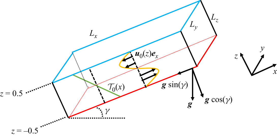


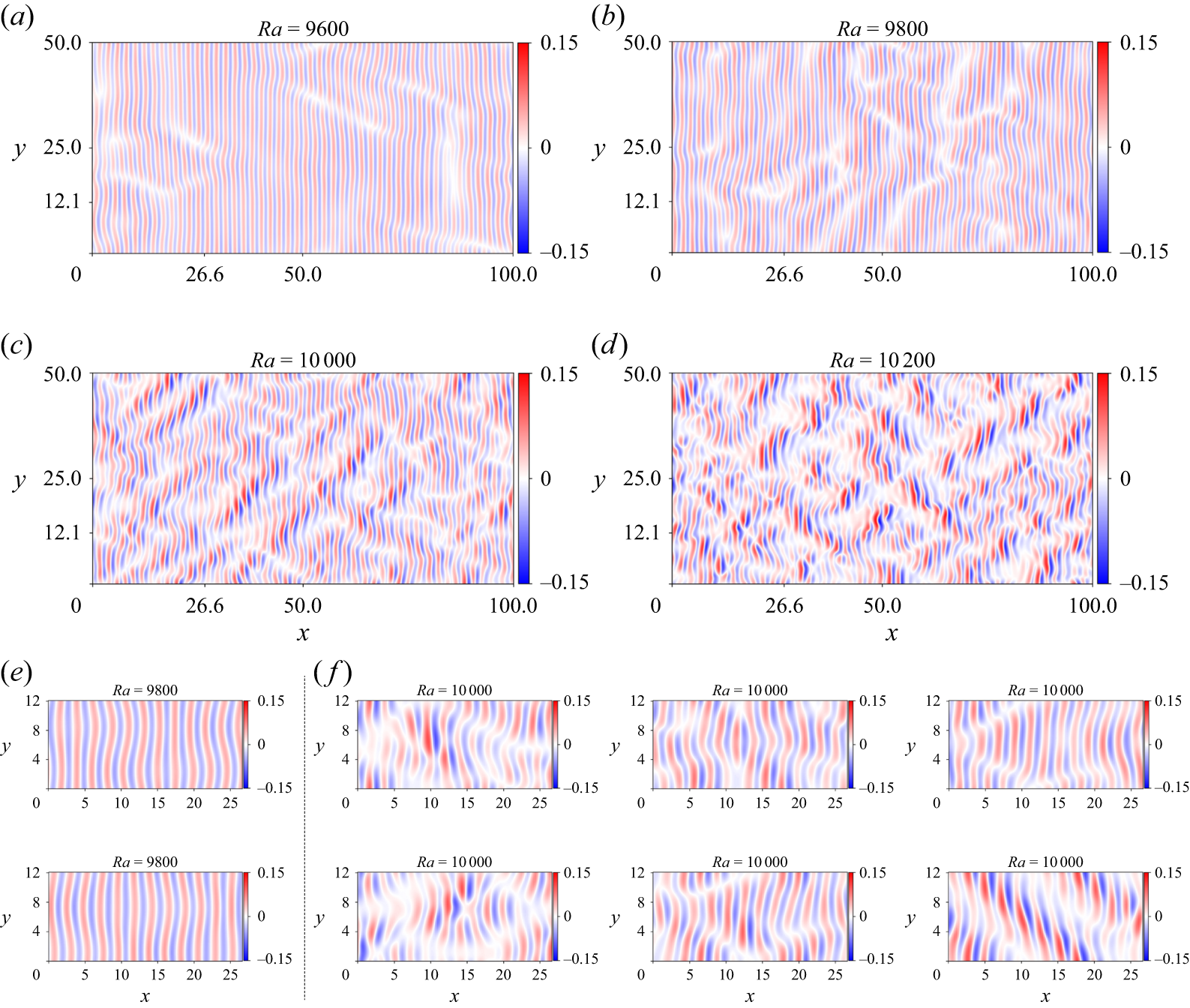


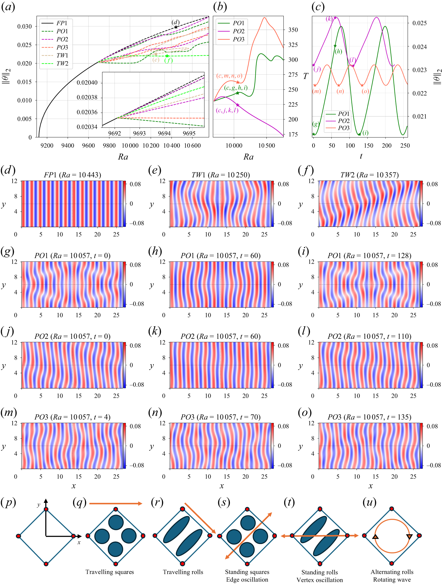


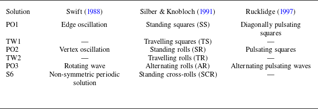
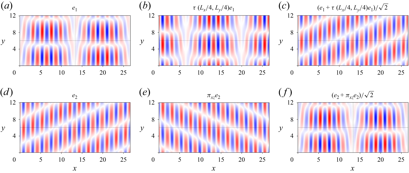


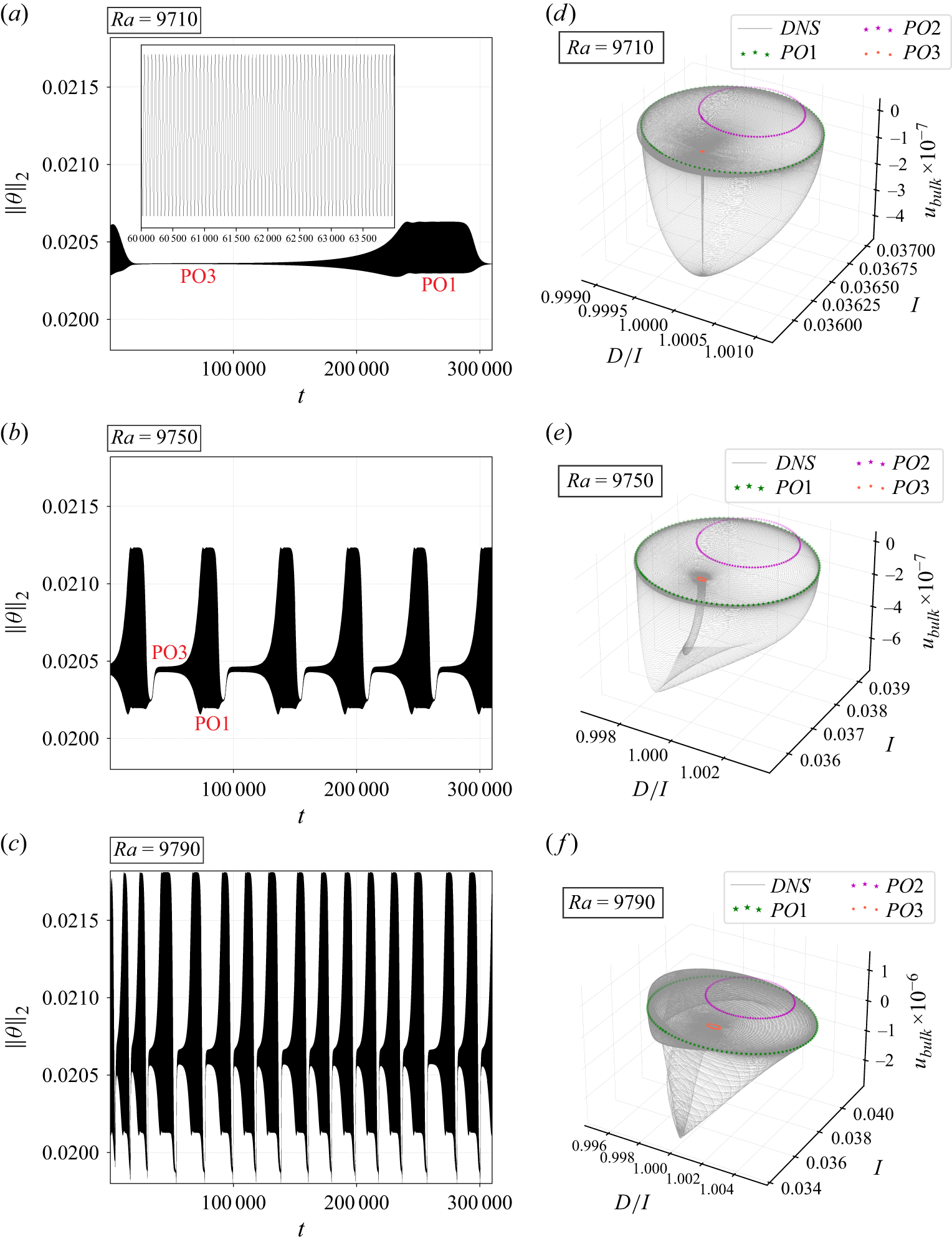


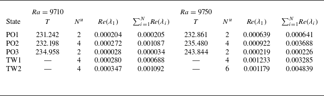


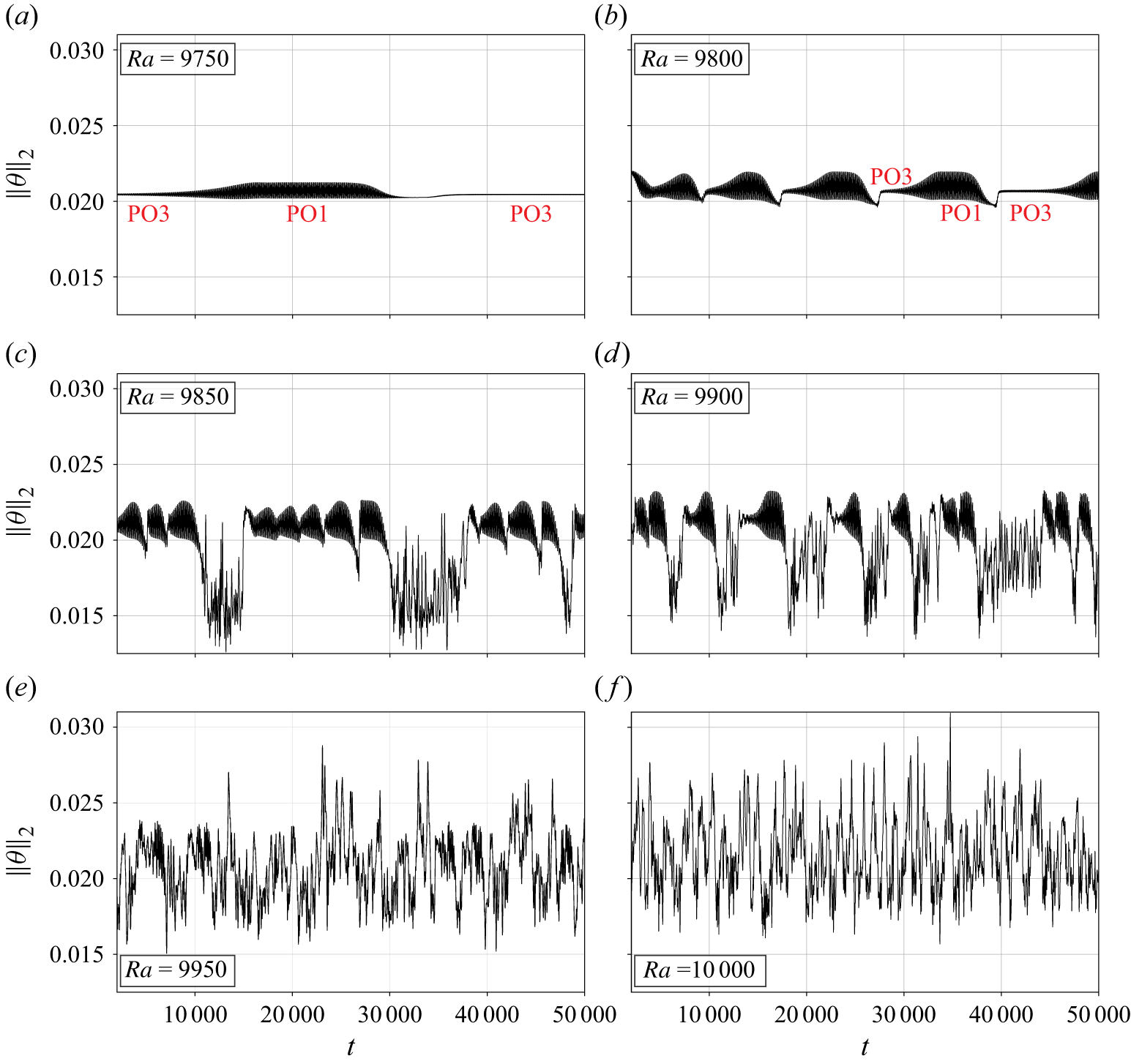


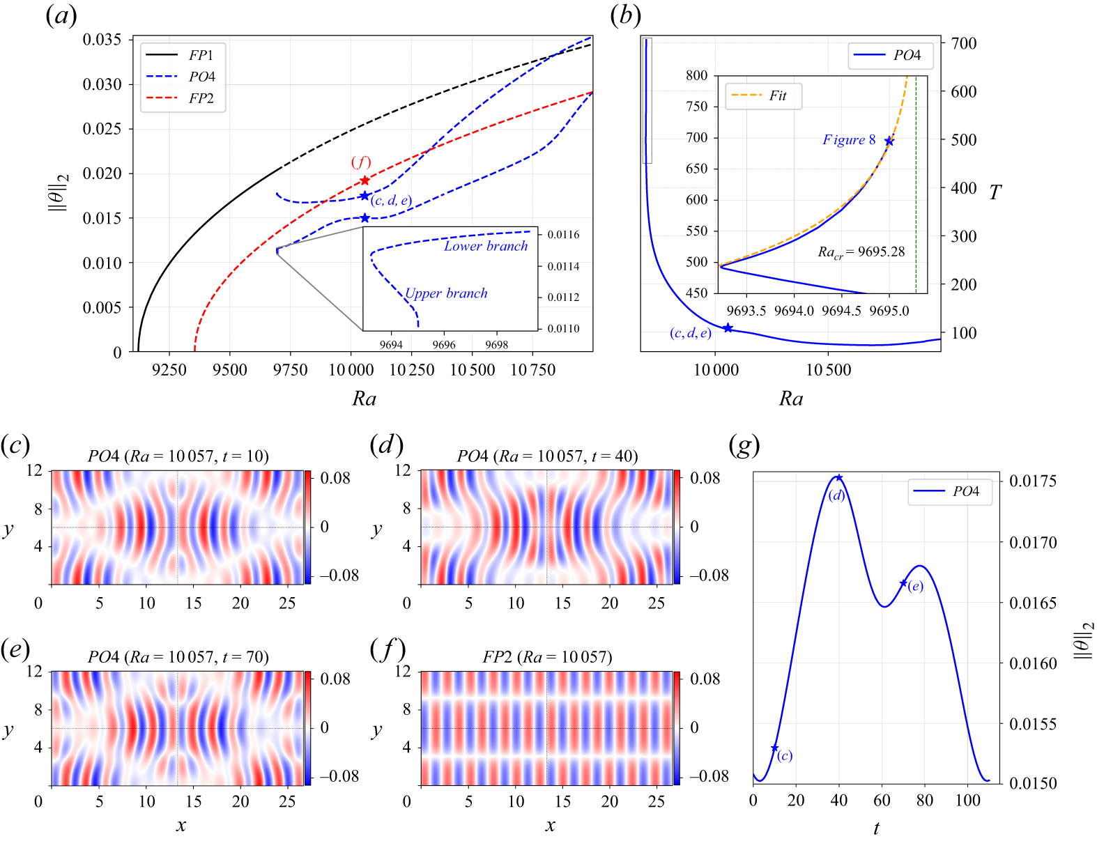


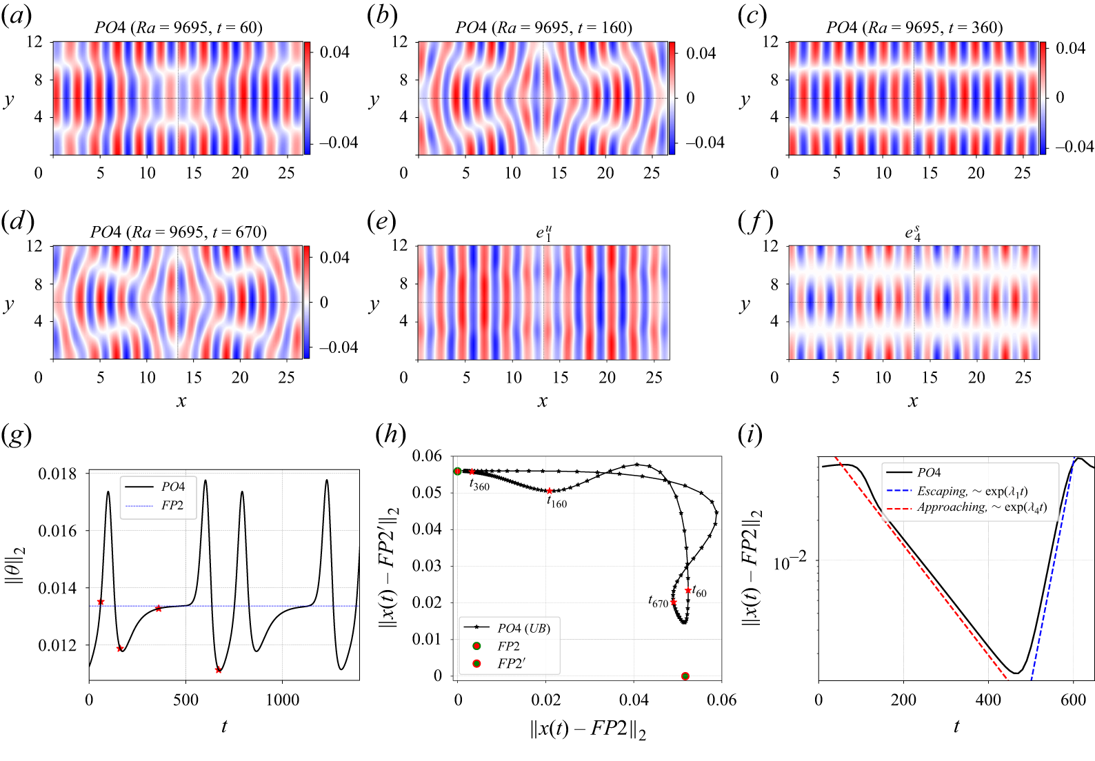


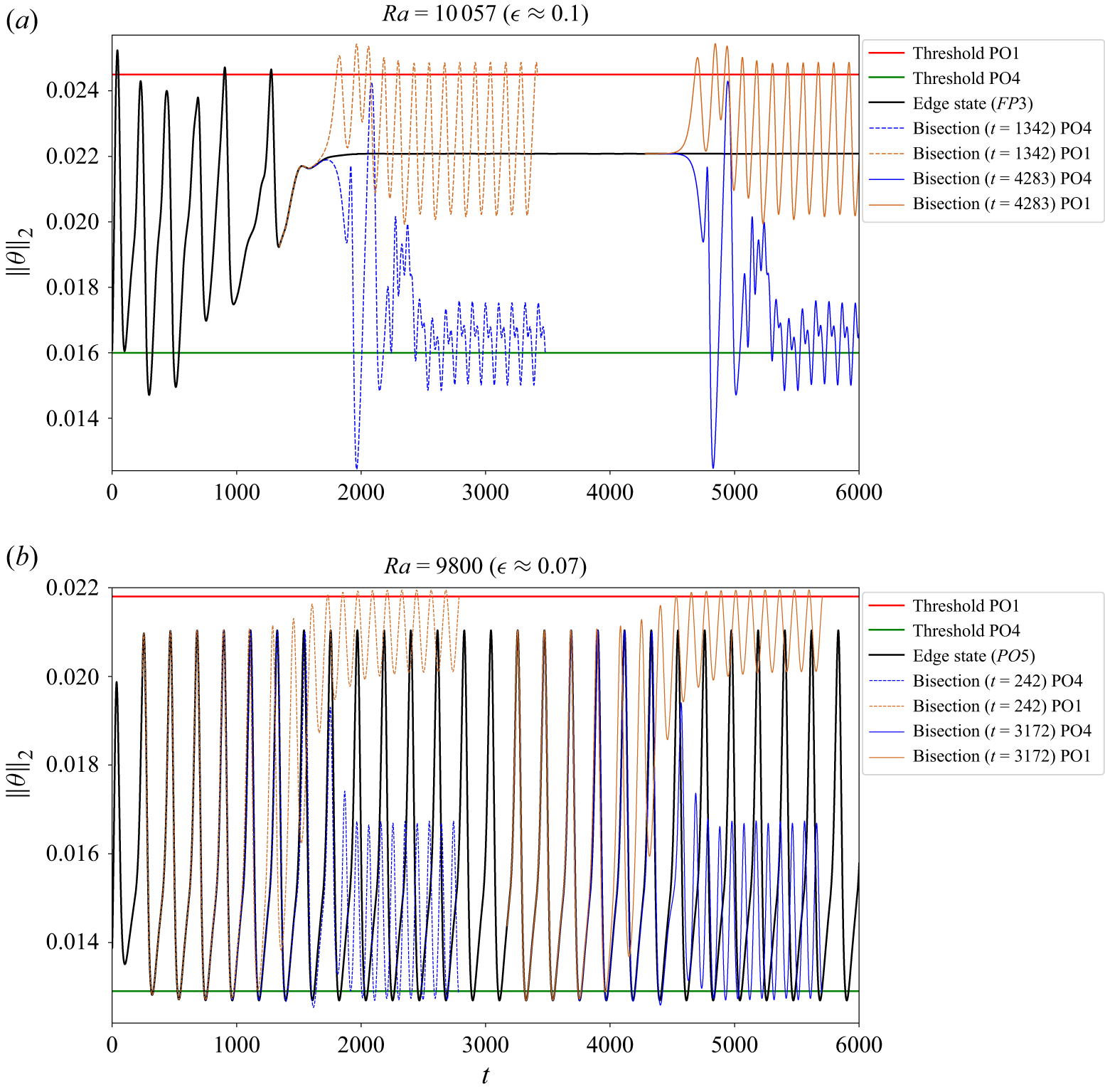


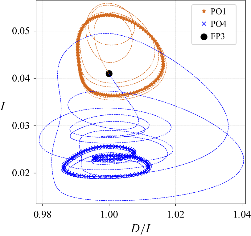


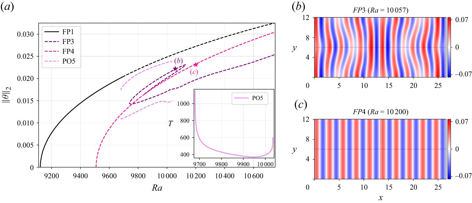
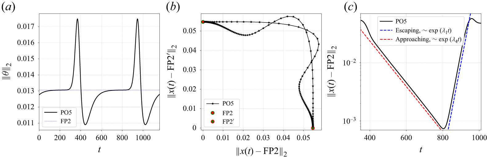


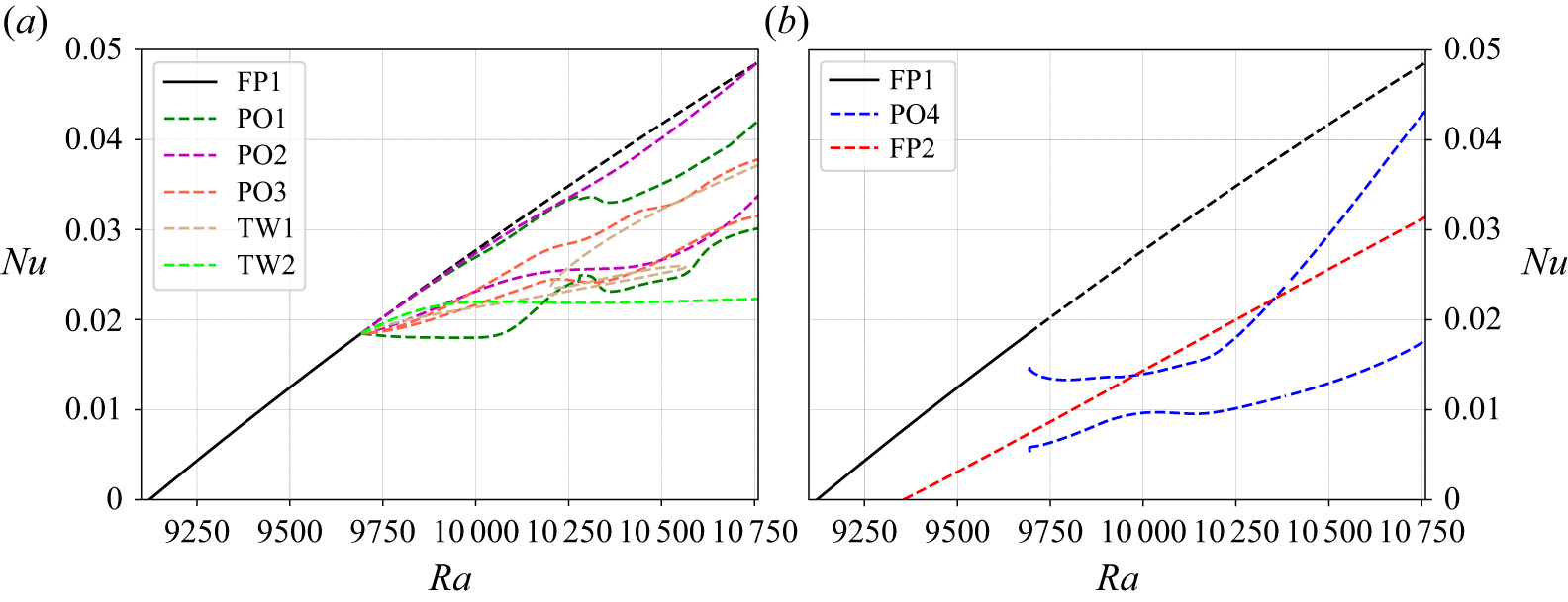

 Open access

