





1. Introduction
Viscoplastic fluids are materials that behave as a solid body as long as the stress remains below the yield stress, and as a viscous fluid above this threshold. Many geophysical mass flows such as avalanches, mud and lava flows involve yield-stress behaviour (Ancey Reference Ancey2007). Biological materials such as blood clots or mucus can be viscoplastic, causing relevant problems in medicine (Balmforth, Frigaard & Ovarlez Reference Balmforth, Frigaard and Ovarlez2014). Engineering applications such as inkjet printing, the creation of chocolate confections or concrete, all have to deal with the viscoplastic behaviour (Bird et al. Reference Bird, Dai, Yarusso and Bird1983). In this work, we consider free-surface flows of idealized viscoplastic fluids down an inclined plane under gravity. Here, idealized viscoplasticity corresponds to a perfectly rigid behaviour in the solid-like regime.
Mathematical modelling of ideal viscoplastic fluid flows generally relies on the Bingham or the Herschel–Bulkley constitutive laws, combined with mass conservation and Cauchy momentum equations. An accurate direct numerical simulation of this problem generally requires large computing times and the use of very fine meshes in the vicinity of yield surfaces separating unyielded (solid-like) from yielded (fluid-like) regions (Frigaard & Nouar Reference Frigaard and Nouar2005; Glowinski & Wachs Reference Glowinski and Wachs2011; Dimakopoulos, Pavlidis & Tsamopoulos Reference Dimakopoulos, Pavlidis and Tsamopoulos2013; Liu, Balmforth & Hormozi Reference Liu, Balmforth and Hormozi2019). Alternatively, approximate models of reduced dimensionality can be considered. For free-surface flows, a thin-layer approximation combined with an integration over the flow depth is the most common approach to derive reduced models. In addition to reducing the number of equations to be solved, this approach also allows the boundary conditions to be directly incorporated into the models.
The thin-layer approach includes one-equation models based on a single mass balance equation (Balmforth et al. Reference Balmforth, Craster, Rust and Sassi2006; Ancey & Cochard Reference Ancey and Cochard2009) and more general shallow-flow models relying on two (Ng & Mei Reference Ng and Mei1994; Fernández-Nieto et al. Reference Fernández-Nieto, Noble and Vila2010; Muchiri, Monnier & Sellier Reference Muchiri, Monnier and Sellier2025) or three equations (Denisenko, Richard & Chambon Reference Denisenko, Richard and Chambon2023). One-equation models have usually simple structures and are easy to implement, however, they might produce diverging or inaccurate solutions when the instability threshold for uniform flows is exceeded (Benney Reference Benney1966; Pumir, Manneville & Pomeau Reference Pumir, Manneville and Pomeau1983; Ooshida Reference Ooshida1999). Two-equation shallow-flow models include inertia and are widely used for many types of fluids. They are typically based on the mass and momentum balance equations. However, these models are generally incompatible with the work–energy theorem (Richard et al. Reference Richard, Gisclon, Ruyer-Quil and Vila2019). This issue can be overcome by using three-equation shallow-flow models, which are usually based on mass, momentum and energy balance equations. Compatibility with the work–energy theorem is guaranteed by the introduction of an enstrophy variable, related to internal shearing of the flow. This approach was initially proposed by Teshukov (Reference Teshukov2007) and successfully applied to viscous fluids by Richard, Ruyer-Quil & Vila (Reference Richard, Ruyer-Quil and Vila2016), to Bingham materials by Denisenko et al. (Reference Denisenko, Richard and Chambon2023) and to granular materials by Deleage & Richard (Reference Deleage and Richard2025). An important advantage of this three-equation approach is the fully hyperbolic structure of the resulting models, which ensures the well-posedness of the problem and allows for efficient computational resolution with robust numerical schemes.
The key parameter in thin-layer approaches is the aspect ratio $\varepsilon = h_0/l_0$
, where
$\varepsilon = h_0/l_0$
, where $h_0$
and
$h_0$
and $l_0$
are the typical depth and length of the flow, respectively. Thin-layer models are derived by averaging the governing equation along the depth, using asymptotic expansions with respect to
$l_0$
are the typical depth and length of the flow, respectively. Thin-layer models are derived by averaging the governing equation along the depth, using asymptotic expansions with respect to $\varepsilon$
. To capture the right physics and properly account for the fluid rheology, the derived models should be consistent at least at order
$\varepsilon$
. To capture the right physics and properly account for the fluid rheology, the derived models should be consistent at least at order $O(\varepsilon )$
. A model is said to be consistent at order
$O(\varepsilon )$
. A model is said to be consistent at order $k$
if the leading terms in the model equations are of
$k$
if the leading terms in the model equations are of $O(1)$
, and if all terms vanish except for a remainder of
$O(1)$
, and if all terms vanish except for a remainder of $O(\varepsilon ^{k+1})$
after having inserted the asymptotic expansions obtained above into the model equations. Many consistent models have been derived for Newtonian (Benney Reference Benney1966; Ruyer-Quil & Manneville Reference Ruyer-Quil and Manneville2000; Usha & Uma Reference Usha and Uma2004; Richard et al. Reference Richard, Ruyer-Quil and Vila2016) or power-law fluid flows (Ruyer-Quil, Chakraborty & Dandapat Reference Ruyer-Quil, Chakraborty and Dandapat2012; Noble & Vila Reference Noble and Vila2013; Boutounet, Monnier & Vila Reference Boutounet, Monnier and Vila2016; Chesnokov Reference Chesnokov2021). However, the derivation of consistent models for viscoplastic fluids remains rare (Balmforth & Liu Reference Balmforth and Liu2004; Fernández-Nieto et al. Reference Fernández-Nieto, Noble and Vila2010; Denisenko et al. Reference Denisenko, Richard and Chambon2023) and is limited to the case of Bingham fluids. Extension of these models to Herschel–Bulkley fluids is challenging due to an additional singularity in the viscous stress tensor and the nonlinear behaviour inherent to power-law rheology. Yet, the Herschel–Bulkley model is better representative of real viscoplastic materials, making such extensions essential for realistic modelling.
$O(\varepsilon ^{k+1})$
after having inserted the asymptotic expansions obtained above into the model equations. Many consistent models have been derived for Newtonian (Benney Reference Benney1966; Ruyer-Quil & Manneville Reference Ruyer-Quil and Manneville2000; Usha & Uma Reference Usha and Uma2004; Richard et al. Reference Richard, Ruyer-Quil and Vila2016) or power-law fluid flows (Ruyer-Quil, Chakraborty & Dandapat Reference Ruyer-Quil, Chakraborty and Dandapat2012; Noble & Vila Reference Noble and Vila2013; Boutounet, Monnier & Vila Reference Boutounet, Monnier and Vila2016; Chesnokov Reference Chesnokov2021). However, the derivation of consistent models for viscoplastic fluids remains rare (Balmforth & Liu Reference Balmforth and Liu2004; Fernández-Nieto et al. Reference Fernández-Nieto, Noble and Vila2010; Denisenko et al. Reference Denisenko, Richard and Chambon2023) and is limited to the case of Bingham fluids. Extension of these models to Herschel–Bulkley fluids is challenging due to an additional singularity in the viscous stress tensor and the nonlinear behaviour inherent to power-law rheology. Yet, the Herschel–Bulkley model is better representative of real viscoplastic materials, making such extensions essential for realistic modelling.
Most models used in practical applications for viscoplastic fluids are inconsistent and generally based on simple, ad hoc closures. In particular, the friction term is often postulated from the relation associated with the leading-order velocity profile. For Bingham fluids, this leads to an analytical expression of the friction term (Huang & Garcia Reference Huang and Garcia1998). However, this expression depends on the unknown position of the yield surface. Pastor et al. (Reference Pastor, Quecedo, González, Herreros, Merodo and Mira2004) expressed this position as a function of the friction, providing a closure more suitable for numerical implementation under the form of a third-order polynomial. For Herschel–Bulkley fluids, this approach leads to a nonlinear algebraic equation that cannot be solved analytically (Ancey, Andreini & Epely-Chauvin Reference Ancey, Andreini and Epely-Chauvin2012). An analytical fit for this equation was proposed by Coussot (Reference Coussot1997) for values of power-law index $n$
close to
$n$
close to $1/3$
. Muchiri et al. (Reference Muchiri, Monnier and Sellier2025) proposed considering a friction term linearly dependent on the velocity. It allows them to write the friction term in an analytical form, but their expression does not coincide with the exact expression of the friction term in the particular case of power-law fluids (Ng & Mei Reference Ng and Mei1994). Generally, inconsistent ad hoc shallow-flow models may demonstrate relatively accurate predictions for the front velocity and free-surface shape (Hogg & Pritchard Reference Hogg and Pritchard2004; Ancey & Cochard Reference Ancey and Cochard2009; Ancey et al. Reference Ancey, Andreini and Epely-Chauvin2012; Saingier, Deboeuf & Lagrée Reference Saingier, Deboeuf and Lagrée2016; Fernández-Nieto et al. Reference Fernández-Nieto, Garres-Díaz and Vigneaux2023; Muchiri et al. Reference Muchiri, Hewett, Sellier, Moyers-Gonzalez and Monnier2024). However, these models usually fail to capture the proper instability threshold of the equilibrium flows (Balmforth & Liu Reference Balmforth and Liu2004; Kalliadasis et al. Reference Kalliadasis, Ruyer-Quil, Scheid and Velarde2012).
$1/3$
. Muchiri et al. (Reference Muchiri, Monnier and Sellier2025) proposed considering a friction term linearly dependent on the velocity. It allows them to write the friction term in an analytical form, but their expression does not coincide with the exact expression of the friction term in the particular case of power-law fluids (Ng & Mei Reference Ng and Mei1994). Generally, inconsistent ad hoc shallow-flow models may demonstrate relatively accurate predictions for the front velocity and free-surface shape (Hogg & Pritchard Reference Hogg and Pritchard2004; Ancey & Cochard Reference Ancey and Cochard2009; Ancey et al. Reference Ancey, Andreini and Epely-Chauvin2012; Saingier, Deboeuf & Lagrée Reference Saingier, Deboeuf and Lagrée2016; Fernández-Nieto et al. Reference Fernández-Nieto, Garres-Díaz and Vigneaux2023; Muchiri et al. Reference Muchiri, Hewett, Sellier, Moyers-Gonzalez and Monnier2024). However, these models usually fail to capture the proper instability threshold of the equilibrium flows (Balmforth & Liu Reference Balmforth and Liu2004; Kalliadasis et al. Reference Kalliadasis, Ruyer-Quil, Scheid and Velarde2012).
The main difficulty in deriving consistent shallow-flow models for Herschel–Bulkley fluids is related to the intricacies of the asymptotic expansion. At leading order with respect to $\varepsilon$
, the velocity expansion describes a yielded layer at the base of the flow, overlaid by a rigid plug close to the free surface (Coussot Reference Coussot1994; Chambon, Ghemmour & Laigle Reference Chambon, Ghemmour and Laigle2009). However, at the next order, this plug layer happens to be a pseudoplug in which the strain rate is of order
$\varepsilon$
, the velocity expansion describes a yielded layer at the base of the flow, overlaid by a rigid plug close to the free surface (Coussot Reference Coussot1994; Chambon, Ghemmour & Laigle Reference Chambon, Ghemmour and Laigle2009). However, at the next order, this plug layer happens to be a pseudoplug in which the strain rate is of order $O(\varepsilon )$
(Balmforth & Craster Reference Balmforth and Craster1999; Chambon et al. Reference Chambon, Freydier, Naaim and Vila2020). The strain rate thus derived diverges at the interface between the pseudoplug and the sheared layer, resulting in a non-smooth velocity profile. While it is possible to employ this expansion for deriving a consistent shallow-flow model (Fernández-Nieto et al. Reference Fernández-Nieto, Noble and Vila2010), this model is characterized by a complex mathematical structure and exhibits an unphysical destabilizing effect of plasticity at large angles, predicting an absolutely unstable rigid layer at the plastic limit (Denisenko et al. Reference Denisenko, Richard and Chambon2023). A smooth expression for the velocity field, avoiding divergence of the strain rate, can be obtained through an asymptotic matching procedure that introduces an additional transition layer and includes extra terms of higher orders (Fernández-Nieto et al. Reference Fernández-Nieto, Noble and Vila2010; Denisenko, Richard & Chambon Reference Denisenko, Richard and Chambon2025). However, these extra terms are given by non-integrable expressions, preventing one from deriving a traceable shallow-flow model. In our recent paper (Denisenko et al. Reference Denisenko, Richard and Chambon2025) we proposed an alternative path to construct a smooth velocity expansion given by fully analytical expressions, based on an alternative tensorial extension of the Herschel–Bulkley law. In the case of Bingham fluids, this approach was already successfully used to derive a three-equation shallow-flow model with a good mathematical structure (Denisenko et al. Reference Denisenko, Richard and Chambon2023).
$O(\varepsilon )$
(Balmforth & Craster Reference Balmforth and Craster1999; Chambon et al. Reference Chambon, Freydier, Naaim and Vila2020). The strain rate thus derived diverges at the interface between the pseudoplug and the sheared layer, resulting in a non-smooth velocity profile. While it is possible to employ this expansion for deriving a consistent shallow-flow model (Fernández-Nieto et al. Reference Fernández-Nieto, Noble and Vila2010), this model is characterized by a complex mathematical structure and exhibits an unphysical destabilizing effect of plasticity at large angles, predicting an absolutely unstable rigid layer at the plastic limit (Denisenko et al. Reference Denisenko, Richard and Chambon2023). A smooth expression for the velocity field, avoiding divergence of the strain rate, can be obtained through an asymptotic matching procedure that introduces an additional transition layer and includes extra terms of higher orders (Fernández-Nieto et al. Reference Fernández-Nieto, Noble and Vila2010; Denisenko, Richard & Chambon Reference Denisenko, Richard and Chambon2025). However, these extra terms are given by non-integrable expressions, preventing one from deriving a traceable shallow-flow model. In our recent paper (Denisenko et al. Reference Denisenko, Richard and Chambon2025) we proposed an alternative path to construct a smooth velocity expansion given by fully analytical expressions, based on an alternative tensorial extension of the Herschel–Bulkley law. In the case of Bingham fluids, this approach was already successfully used to derive a three-equation shallow-flow model with a good mathematical structure (Denisenko et al. Reference Denisenko, Richard and Chambon2023).
The goal of this paper is to derive a consistent three-equation shallow-flow model based on the alternative tensorial extension of the Herschel–Bulkley law. The three-equation approach of Richard et al. (Reference Richard, Ruyer-Quil and Vila2016) is important to get the compatibility with the depth-averaged energy equation, while employing the new asymptotic expansion of Denisenko et al. (Reference Denisenko, Richard and Chambon2025) is crucial to obtain a physical instability threshold. The model is derived by averaging the mass, momentum and energy equations. The final result is a hyperbolic system with relaxation source terms, allowing robust numerical schemes to be employed. The influence of the yield-stress and shear-thinning effects on the instability criterion and roll waves are investigated. Importantly, the model is adapted to handle dry fronts and stoppage of the material. These properties are generally lacking in existing consistent shallow-flow models. Comparisons with dam-break experiments are performed. The final plastic shapes of the fluid are studied.
The structure of the paper is the following. In § 2, we present the alternative tensorial extension of the Herschel–Bulkley constitutive law and formulate the governing equations for the fluid flow motion. In § 3, we provide the expression for the long-wave asymptotic expansion ensuring a smooth velocity field. In § 4, a consistent three-equation shallow-flow model is derived from the asymptotic expansion. Section 5 presents applications to various flow configurations, including uniform flow instability, the dam-break problem and flow stoppage. Lastly, in § 6, the influence of selecting different source terms is examined by comparing results for steady-state surges.
2. Statement of the problem
We study a two-dimensional gravity-driven flow of a viscoplastic fluid down an inclined plane (figure 1). The angle of the plane to the horizontal is denoted by $\theta$
. The gravity vector is
$\theta$
. The gravity vector is $\boldsymbol g$
. The
$\boldsymbol g$
. The $x$
- and
$x$
- and $z$
-axes are parallel and orthogonal to the plane, respectively. The components of the velocity
$z$
-axes are parallel and orthogonal to the plane, respectively. The components of the velocity $\boldsymbol{{v}}$
along the
$\boldsymbol{{v}}$
along the $x$
and
$x$
and $z$
directions are denoted
$z$
directions are denoted $u$
and
$u$
and $w$
. The components of the strain-rate tensor
$w$
. The components of the strain-rate tensor $\dot {\boldsymbol{\gamma }}$
are defined as
$\dot {\boldsymbol{\gamma }}$
are defined as $\dot \gamma _{xx} = 2 \partial u / \partial x$
,
$\dot \gamma _{xx} = 2 \partial u / \partial x$
, $\dot \gamma _{xz} =\partial u/\partial z + \partial w /\partial x$
,
$\dot \gamma _{xz} =\partial u/\partial z + \partial w /\partial x$
, $\dot \gamma _{zz} = 2 \partial w /\partial x$
. The fluid depth is denoted by
$\dot \gamma _{zz} = 2 \partial w /\partial x$
. The fluid depth is denoted by $h(x,t)$
. The fluid is incompressible (
$h(x,t)$
. The fluid is incompressible ( $\text{tr} \, \dot {\boldsymbol \gamma } = 0$
) with a density
$\text{tr} \, \dot {\boldsymbol \gamma } = 0$
) with a density $\rho$
and a pressure
$\rho$
and a pressure $p$
.
$p$
.
Definition sketch.

2.1. Constitutive law
A generalized tensorial extension of the Herschel–Bulkley constitutive law within the framework of the shallow-flow asymptotic expansion has been proposed in our recent work (Denisenko et al. Reference Denisenko, Richard and Chambon2025). Namely, the extra-stress tensor $\boldsymbol{\tau }$
is expressed as
$\boldsymbol{\tau }$
is expressed as
 \begin{align} \tau _{\textit{ij}} = {\tau }_{\textit{ij}}^Y \displaystyle + K{|\dot {\boldsymbol{\gamma }}|^{n-1}}\dot { \gamma }_{\textit{ij}} \qquad & |\dot {\boldsymbol{\gamma }}|\gt 0, \end{align}
 \begin{align} \dot {{\gamma }}_{\textit{ij}} = 0 \qquad & |\boldsymbol \tau | \leqslant \tau _c. \end{align}
The parameters $K$
and
$K$
and $n$
are the consistency and the power index of the material, respectively. The tensor
$n$
are the consistency and the power index of the material, respectively. The tensor $\boldsymbol{\tau }^Y$
is called the yield-stress tensor. The norm is defined as
$\boldsymbol{\tau }^Y$
is called the yield-stress tensor. The norm is defined as $ |\boldsymbol{T}| = (0.5\boldsymbol{T}_{\textit{ij}}\boldsymbol{T}_{\textit{ij}} )^{0.5}$
for any second-order tensor. Hereinafter, for
$ |\boldsymbol{T}| = (0.5\boldsymbol{T}_{\textit{ij}}\boldsymbol{T}_{\textit{ij}} )^{0.5}$
for any second-order tensor. Hereinafter, for $|\boldsymbol \tau | \gt \tau _c$
, we split the extra-stress in its yield-stress and viscous contributions as
$|\boldsymbol \tau | \gt \tau _c$
, we split the extra-stress in its yield-stress and viscous contributions as
 \begin{align} \tau _{\textit{ij}}=\tau _{\textit{ij}}^Y+\tau _{\textit{ij}}^{v}, \quad \tau _{\textit{ij}}^{v}=K\dot {\gamma }_{\textit{ij}}|\dot {{\boldsymbol \gamma }}|^{n-1}. \end{align}
Unlike in the classical tensorial extension of the Herschel–Bulkley rheology, here the yield-stress tensor is not assumed to be aligned with the strain-rate tensor via the expression $\tau _{\textit{ij}}^Y = \tau _c { {\dot {\gamma }_{\textit{ij}}}}/|{\boldsymbol{\dot \gamma }}|$
. We instead define the yield-stress tensor
$\tau _{\textit{ij}}^Y = \tau _c { {\dot {\gamma }_{\textit{ij}}}}/|{\boldsymbol{\dot \gamma }}|$
. We instead define the yield-stress tensor $\boldsymbol{\tau }^{Y}$
based on the following criteria.
$\boldsymbol{\tau }^{Y}$
based on the following criteria.
-
(i) The norm of $\boldsymbol{\tau ^Y}$
is equal to the yield stress
$\tau _c$
in the yielded regime:
$|\boldsymbol{\tau ^Y}|=\tau _c$
. This corresponds to the von Mises yielding criterion.
$\boldsymbol{\tau ^Y}$
is equal to the yield stress
$\tau _c$
in the yielded regime:
$|\boldsymbol{\tau ^Y}|=\tau _c$
. This corresponds to the von Mises yielding criterion. -
(ii) The trace of
$\boldsymbol{\tau ^Y}$
is zero in relation to the incompressibility assumption:
$\mathrm{tr}\, \boldsymbol{\tau ^Y}=0$
. -
(iii) There are no normal stress differences in simple shear, such that
$\boldsymbol{\tau ^Y}$
is aligned with
$\boldsymbol{\dot {\gamma }}/|\boldsymbol{\dot {\gamma }}|$
in the particular case of simple shear flows. Although questionable, this assumption is made to obtain the same leading-order solution as in models based on the classical formulation of the rheology. -
(iv) The existence of a normal stress difference in the pseudoplug at leading order (see below), and all terms originating from these normal stresses in the asymptotic expansions at
$O(\varepsilon )$
, are attributed to the yield-stress tensor and not to the viscous-stress tensor
$\tau ^{v}=K\dot {\gamma }|\dot {{\boldsymbol \gamma }}|^{n-1}$
. All other terms in the asymptotic expansions are attributed to the viscous-stress tensor.


The constitutive law (2.1) together with these four conditions can be viewed as an alternative extension of the one-dimensional Herschel–Bulkley law for two-dimensional shallow flows, since the classical scalar expression $\tau _{xz}=\tau _c+\dot \gamma ^n$
is recovered in simple-shear flows. The fourth condition here can be interpreted as a closure assumption ensuring that the normal stress differences associated with the perfectly rigid regime do not influence the fluid-like dynamics. It avoids the spurious destabilizing effects of plasticity at large slope angles that are observed in the model based on the classical tensorial law (Denisenko et al. Reference Denisenko, Richard and Chambon2023). It is important to emphasize that the four conditions formulated above are meaningful only in the shallow-flow regime, where a dominant direction can be identified and the flow is close to one-dimensional. Although these conditions are not sufficient to fully determine the yield-stress tensor in a general flow, they are sufficient to work out a thin-layer asymptotic expansion up to
$\tau _{xz}=\tau _c+\dot \gamma ^n$
is recovered in simple-shear flows. The fourth condition here can be interpreted as a closure assumption ensuring that the normal stress differences associated with the perfectly rigid regime do not influence the fluid-like dynamics. It avoids the spurious destabilizing effects of plasticity at large slope angles that are observed in the model based on the classical tensorial law (Denisenko et al. Reference Denisenko, Richard and Chambon2023). It is important to emphasize that the four conditions formulated above are meaningful only in the shallow-flow regime, where a dominant direction can be identified and the flow is close to one-dimensional. Although these conditions are not sufficient to fully determine the yield-stress tensor in a general flow, they are sufficient to work out a thin-layer asymptotic expansion up to $O(\varepsilon )$
.
$O(\varepsilon )$
.
The conditions on $\tau _{\textit{ij}}^{Y}$
formulated above were first proposed in Denisenko et al. (Reference Denisenko, Richard and Chambon2023) to avoid the singularity of the yield-stress tensor for
$\tau _{\textit{ij}}^{Y}$
formulated above were first proposed in Denisenko et al. (Reference Denisenko, Richard and Chambon2023) to avoid the singularity of the yield-stress tensor for $|\boldsymbol{\dot {\gamma }}|=0$
. This allowed us to derive a consistent three-equation shallow-flow model for Bingham fluids with a smooth velocity field and a physically correct instability threshold. Later these conditions were used in the derivation of a smooth asymptotic expansion for Herschel–Bulkley fluids (Denisenko et al. Reference Denisenko, Richard and Chambon2025). Here we build on these previous developments to derive a consistent three-equation shallow-flow model in the Herschel–Bulkley case.
$|\boldsymbol{\dot {\gamma }}|=0$
. This allowed us to derive a consistent three-equation shallow-flow model for Bingham fluids with a smooth velocity field and a physically correct instability threshold. Later these conditions were used in the derivation of a smooth asymptotic expansion for Herschel–Bulkley fluids (Denisenko et al. Reference Denisenko, Richard and Chambon2025). Here we build on these previous developments to derive a consistent three-equation shallow-flow model in the Herschel–Bulkley case.
2.2. Governing equations
The continuity equation (mass conservation balance) reads
 \begin{align} \frac {\partial u}{\partial x} + \frac {\partial w}{\partial y}=0. \end{align}
The Cauchy momentum equations in the $x$
and
$x$
and $z$
directions read
$z$
directions read
 \begin{align} \rho \left ( \frac {\partial u}{\partial t} + u\frac {\partial u}{\partial x} + w\frac {\partial u}{\partial z} \right ) = -\frac {\partial p}{\partial x} + \rho g \sin {\theta } +\frac {\partial \tau _{xz}}{\partial z} +\frac {\partial \tau _{xx}}{\partial x}, \end{align}
 \begin{align} \rho \left ( \frac {\partial w}{\partial t} + u \frac {\partial w}{\partial x} + w \frac {\partial w}{\partial z} \right ) = -\frac {\partial p}{\partial z} -\rho g \cos {\theta } +\frac {\partial \tau _{xz}}{\partial x} +\frac {\partial \tau _{xx}}{\partial z}. \end{align}
At the bottom, no-penetration and no-slip boundary conditions are assumed:
 \begin{align} u_{|_{z=0}}=w_{|_{z=0}}=0. \end{align}
At the free surface, the kinematic boundary condition is given by
 \begin{align} \frac {\partial h}{\partial t} + u_{|_{z=h(x)}}\frac {\partial h}{\partial x} =w_{|_{z=h(x)}}, \end{align}
while the dynamic boundary conditions are
 \begin{align} \left [ \displaystyle 1- \left ( \frac {\partial h}{\partial x} \right )^2 \right ]\tau _{xz|_{z=h(x)}} = 2 \displaystyle \left (\frac {\partial h}{\partial x}\right ) \tau _{xx|_{z=h(x)}},\end{align}
 \begin{align} \left [ \displaystyle 1- \left ( \frac {\partial h}{\partial x} \right )^2 \right ] p_{|_{z=h(x)}} = - \left [1+ \displaystyle \left (\frac {\partial h}{\partial x} \right )^2 \right ] \tau _{xx|_{z=h(x)}}.\end{align}
Note that capillarity is neglected in this study. The atmospheric pressure is taken constant and equal to zero.
2.3. Shallow-flow scaling
Let us denote by $h_0$
the characteristic length in
$h_0$
the characteristic length in $z$
direction, by
$z$
direction, by $l_0$
the characteristic length in
$l_0$
the characteristic length in $x$
direction and by
$x$
direction and by $u_0$
the characteristic velocity in
$u_0$
the characteristic velocity in $x$
direction. The shallow-flow hypothesis implies that the aspect ratio
$x$
direction. The shallow-flow hypothesis implies that the aspect ratio $\varepsilon = h_0/l_0$
is small. The relevant dimensionless groups of the problem are the Reynolds number
$\varepsilon = h_0/l_0$
is small. The relevant dimensionless groups of the problem are the Reynolds number $ \textit{Re}$
, the Froude number
$ \textit{Re}$
, the Froude number $ \textit{Fr}$
and the Bingham number
$ \textit{Fr}$
and the Bingham number $ \textit{Bi}$
:
$ \textit{Bi}$
:
 \begin{align} \textit{Re} = \frac {\rho u_0^{2-n}h_0^{n}}{K}, \qquad Fr = \frac {u_0}{\sqrt {gh_0\cos \theta }}, \qquad \textit{Bi} = \frac {\tau _c}{K} \left (\frac {h_0}{u_0}\right )^n. \qquad \end{align}
In this study, these parameters and the slope angle $\theta$
are assumed to be
$\theta$
are assumed to be $O(1)$
with respect to
$O(1)$
with respect to $\varepsilon$
. To rewrite the problem (2.4)–(2.10) into a dimensionless form, the flow variables are expressed as
$\varepsilon$
. To rewrite the problem (2.4)–(2.10) into a dimensionless form, the flow variables are expressed as
 \begin{align} x = l_0{x^\prime}; \quad z = h_0{z^\prime}; \quad u = u_0{u^\prime}; \quad w = \varepsilon u_0 {w^\prime}; \quad t = \frac {l_0}{u_0} {t^\prime}; \quad h = u_0 {h^\prime}; \nonumber \\ p = \rho g h_0\cos \theta {p^\prime}; \quad \tau _{\textit{ij}} = \tau _c {\tau ^\prime}_{\textit{ij}}; \quad |\boldsymbol \tau | =\tau _c|{\boldsymbol \tau }^\prime|; \quad |\dot {\boldsymbol{\gamma }}| = \frac {u_0}{h_0}|\dot {{\boldsymbol{\gamma }}}^\prime|. \end{align}
For convenience, we shall further omit the primes. The continuity (2.4) keeps the form
 \begin{align} \frac {\partial u}{\partial x} + \frac {\partial w}{\partial y}=0, \end{align}
while the scaled momentum (2.5)–(2.6) take the following form:
 \begin{align} \varepsilon \left (\frac {\partial u}{\partial t} + {u}\frac {\partial u}{\partial x} + {w}\frac {\partial u}{\partial z}\right ) = - \frac {\varepsilon }{Fr^2} \frac {\partial p}{\partial x} + \frac {\lambda }{ \textit{Re}} + \frac {\textit{Bi}}{ \textit{Re}} \frac {\partial \tau _{xz}}{\partial z} + \frac {\varepsilon \textit{Bi}}{\textit{Re}}\frac {\partial \tau _{xx}}{\partial x},\end{align}
 \begin{align} \varepsilon ^2 \left ( \frac {\partial w}{\partial t} + {u} \frac {\partial w}{\partial x} + {w} \frac {\partial w}{\partial z} \right ) = -\frac {1}{Fr^2} \left ( 1+\frac {\partial p}{\partial z} \right ) + \frac {\varepsilon \textit{Bi}}{\textit{Re}} \frac {\partial \tau _{xz}}{\partial x} + \frac {\textit{Bi}}{\textit{Re}}\frac {\partial \tau _{zz}}{\partial z},\end{align}
with the driving parameter $\lambda$
given by
$\lambda$
given by
 \begin{align} \lambda = \frac {\rho g h_0^{n+1} \sin {\theta }}{K{u}_0^n}=\frac {\textit{Re}}{Fr^2}\tan {\theta }. \end{align}
In the scaled variables, the yielding criterion reduces to $|\boldsymbol \tau |=1$
. For
$|\boldsymbol \tau |=1$
. For $|\boldsymbol \tau |\gt 1$
, the expressions for the viscous and yield-stress components of (2.3) are transformed to
$|\boldsymbol \tau |\gt 1$
, the expressions for the viscous and yield-stress components of (2.3) are transformed to
 \begin{align} {\tau }_{xx} = {\tau }_{xx}^Y + {\tau }_{xx}^{v}, \qquad {\tau }_{xx}^{v} = \frac {2\varepsilon }{\textit{Bi}} \frac {\partial u}{\partial x}| {\boldsymbol{{\dot \gamma }}}|^{n-1},\end{align}
 \begin{align} {\tau }_{xz} = {\tau }_{xz}^Y + {\tau }_{xz}^{v}, \qquad {\tau }_{xz}^{v} = \frac {1}{\textit{Bi}}\left (\frac {\partial u}{\partial z} +\varepsilon ^2 \frac {\partial w}{\partial x} \right ) | {\boldsymbol{{\dot \gamma }}}|^{n-1}.\end{align}
The condition on the norm of the dimensionless yield-stress tensor is
 \begin{align} \left ({\tau }_{xx}^Y\right )^2 + \left ({\tau }_{xz}^Y\right )^2=1. \end{align}
The no-penetration and no-slip conditions (2.7) keep the same form,
 \begin{align} {u}_{|_{{z}=0}}={w}_{|_{{z}=0}}=0, \end{align}
while the scaled kinematic and dynamic boundary conditions (2.8)–(2.10) are rewritten as
 \begin{align} \frac {\partial h}{\partial x} + {u}_{|_{{z}={h}({x})}}\frac {\partial h}{\partial x} ={w}_{|_{{z}={h}({x})}},\end{align}
 \begin{align} \left [ \displaystyle 1- \varepsilon ^2\left ( \frac {\partial h}{\partial x} \right )^2 \right ]{\tau _{xz}}_{|_{{z}={h}({x})}} = 2 \varepsilon \left (\frac {\partial h}{\partial x}\right ) {\tau _{xx}}_{|_{{z}={h}({x})}},\end{align}
 \begin{align} \left [ 1-\varepsilon ^2 \left ( \frac {\partial h}{\partial x} \right )^2 \right ] {p}_{|_{{z}={h}({x})}} = -\frac {\textit{Bi} Fr^2}{\textit{Re}} \left [1+ \varepsilon ^2\left (\frac {\partial h}{\partial x} \right )^2 \right ] {{\tau }_{xx}}_{|_{{z}={h}({x})}}.\end{align}
Finally, the norms of the dimensionless stress and strain-rate tensors read
 \begin{align} |{\boldsymbol \tau }| = \sqrt {{\tau }_{xx}^2+{\tau }_{xz}^2}, \qquad |{\boldsymbol{{\dot \gamma }}}| = \sqrt { \left ( {\partial _z {u}} + \varepsilon ^2 {\partial _x {w}} \right )^2 + 4\varepsilon ^2 \left ( {\partial _x {u}} \right )^2 }. \end{align}
3. Asymptotic expansion
Asymptotic expansions of the flow variables for the alternative rheology (2.1)–(2.2) have been derived up to $O(\varepsilon )$
in our recent paper (Denisenko et al. Reference Denisenko, Richard and Chambon2025). All variables are expanded as
$O(\varepsilon )$
in our recent paper (Denisenko et al. Reference Denisenko, Richard and Chambon2025). All variables are expanded as
 \begin{align} f =f^{(0)}+\varepsilon f^{(1)}+O(\varepsilon ^2). \end{align}
The detailed expressions of these expansions are given in Appendix A. Here we only recall the structure and key properties of the longitudinal velocity expansion.
At leading order, the term $u^{(0)}$
coincides with the expression obtained for the classical Herschel–Bulkley constitutive law, as considered in many studies (e.g. Coussot Reference Coussot1994; Chambon et al. Reference Chambon, Ghemmour and Laigle2009). It corresponds to a sheared layer at the base of the flow, overlaid by a rigid plug close to the free surface. The thickness of the plug is
$u^{(0)}$
coincides with the expression obtained for the classical Herschel–Bulkley constitutive law, as considered in many studies (e.g. Coussot Reference Coussot1994; Chambon et al. Reference Chambon, Ghemmour and Laigle2009). It corresponds to a sheared layer at the base of the flow, overlaid by a rigid plug close to the free surface. The thickness of the plug is $h_p=\textit{Bi}/\lambda$
. In this plug the stress is at the yielding point
$h_p=\textit{Bi}/\lambda$
. In this plug the stress is at the yielding point $|\boldsymbol{\tau }|=\tau _c$
due to the contribution of the plastic normal stresses. At the next order, the plug layer is treated as a pseudoplug, characterized by a strain rate of order
$|\boldsymbol{\tau }|=\tau _c$
due to the contribution of the plastic normal stresses. At the next order, the plug layer is treated as a pseudoplug, characterized by a strain rate of order $O(\varepsilon )$
. This idea was proposed by Balmforth & Craster (Reference Balmforth and Craster1999) in order to allow the asymptotic expansion to be carried out.
$O(\varepsilon )$
. This idea was proposed by Balmforth & Craster (Reference Balmforth and Craster1999) in order to allow the asymptotic expansion to be carried out.
At first order, the correction $u^{(1)}$
consists of two contributions. The first contribution is identical to the result derived for the classical Herschel–Bulkley constitutive law under the assumption of zero shearing in the pseudoplug, obtained by Balmforth & Liu (Reference Balmforth and Liu2004). The second contribution depends on an additional parameter
$u^{(1)}$
consists of two contributions. The first contribution is identical to the result derived for the classical Herschel–Bulkley constitutive law under the assumption of zero shearing in the pseudoplug, obtained by Balmforth & Liu (Reference Balmforth and Liu2004). The second contribution depends on an additional parameter $\delta$
and arises as a result of the ‘Bingham plateau’ regularization, which is introduced at
$\delta$
and arises as a result of the ‘Bingham plateau’ regularization, which is introduced at $O(\varepsilon )$
for
$O(\varepsilon )$
for $n\lt 1$
in order to suppress the divergence of the local effective viscosity and to allow for non-zero shearing in the pseudoplug. This regularization is required to obtain asymptotic expansions in a closed analytical form with the alternative tensorial constitutive law used here, and only concerns the viscous stress tensor, such that the material remains perfectly rigid below the yielding threshold (for more details see Denisenko et al. (Reference Denisenko, Richard and Chambon2025)). Importantly, applying this regularization at
$n\lt 1$
in order to suppress the divergence of the local effective viscosity and to allow for non-zero shearing in the pseudoplug. This regularization is required to obtain asymptotic expansions in a closed analytical form with the alternative tensorial constitutive law used here, and only concerns the viscous stress tensor, such that the material remains perfectly rigid below the yielding threshold (for more details see Denisenko et al. (Reference Denisenko, Richard and Chambon2025)). Importantly, applying this regularization at $O(\varepsilon )$
, rather than at
$O(\varepsilon )$
, rather than at $O(1)$
, is beneficial, as it does not affect the leading-order expression and allows us to recover the classical Herschel–Bulkley result for
$O(1)$
, is beneficial, as it does not affect the leading-order expression and allows us to recover the classical Herschel–Bulkley result for $u^{(0)}$
. The regularization parameter
$u^{(0)}$
. The regularization parameter $\delta$
is considered to be small and of order
$\delta$
is considered to be small and of order $O(\varepsilon ^{\beta })$
with
$O(\varepsilon ^{\beta })$
with $\beta \gt 0$
, so the total contribution associated with
$\beta \gt 0$
, so the total contribution associated with $\delta$
is of
$\delta$
is of $O(\delta ^{1/n-1} \varepsilon )$
=
$O(\delta ^{1/n-1} \varepsilon )$
= $O(\varepsilon ^{1+\beta (1/n-1)}$
) and it does not formally contribute to the expansions up to
$O(\varepsilon ^{1+\beta (1/n-1)}$
) and it does not formally contribute to the expansions up to $O(\varepsilon )$
.
$O(\varepsilon )$
.
In essence, the parameter $\delta$
allows one to tune the magnitude of a small shear rate in the pseudoplug. In particular, a suitable value of this parameter enables an accurate approximation of the ‘complete’ asymptotic expansion associated with non-integrable equations (for more details Denisenko et al. (Reference Denisenko, Richard and Chambon2025)). However, as shown later, the effect of this parameter on the instability thresholds and free-surface profiles is barely noticeable.
$\delta$
allows one to tune the magnitude of a small shear rate in the pseudoplug. In particular, a suitable value of this parameter enables an accurate approximation of the ‘complete’ asymptotic expansion associated with non-integrable equations (for more details Denisenko et al. (Reference Denisenko, Richard and Chambon2025)). However, as shown later, the effect of this parameter on the instability thresholds and free-surface profiles is barely noticeable.
It should also be noted that the definition of the yield-stress tensor $\boldsymbol{\tau }^{Y}$
through the four conditions (i)–(iv) can thus be considered as a specific type of regularization written in the framework of shallow flows. Indeed, it recovers the classical shallow-flow asymptotic expansion in the fully sheared layer up to
$\boldsymbol{\tau }^{Y}$
through the four conditions (i)–(iv) can thus be considered as a specific type of regularization written in the framework of shallow flows. Indeed, it recovers the classical shallow-flow asymptotic expansion in the fully sheared layer up to $O(\varepsilon )$
; the differences arise only in the pseudoplug region at
$O(\varepsilon )$
; the differences arise only in the pseudoplug region at $O(\varepsilon )$
. However, unlike classical regularizations – where solid behaviour is approximated by a highly viscous fluid – the material here remains truly rigid below the yield point. As a result, the present approach for deriving the tractable asymptotic expansion of viscoplastic fluids combines two distinct types of regularization: one avoids the singularity of the yield-stress tensor by relaxing the general collinearity condition between the yield-stress tensor and the strain-rate tensor and replacing it with additional closure assumptions that allow to preserve the rigid behaviour below the yield point; the other modifies the power-law viscous contribution at
$O(\varepsilon )$
. However, unlike classical regularizations – where solid behaviour is approximated by a highly viscous fluid – the material here remains truly rigid below the yield point. As a result, the present approach for deriving the tractable asymptotic expansion of viscoplastic fluids combines two distinct types of regularization: one avoids the singularity of the yield-stress tensor by relaxing the general collinearity condition between the yield-stress tensor and the strain-rate tensor and replacing it with additional closure assumptions that allow to preserve the rigid behaviour below the yield point; the other modifies the power-law viscous contribution at $O(\varepsilon )$
in the pseudoplug layer by replacing Herschel–Bulkley behaviour with Bingham behaviour, while retaining the full Herschel–Bulkley rheology at leading order.
$O(\varepsilon )$
in the pseudoplug layer by replacing Herschel–Bulkley behaviour with Bingham behaviour, while retaining the full Herschel–Bulkley rheology at leading order.
4. Depth-averaged model
The model is derived by averaging the governing (2.13)–(2.15) over the flow depth, taking into account the boundary conditions at the bottom and at the free surface. The asymptotic expansions presented in the Appendix A are used for neglecting all terms smaller than $O(\varepsilon \delta ^{1/n-1})$
. It should be emphasized that an infinite number of asymptotically consistent models with different source terms can be derived using the asymptotic procedure presented below. However, not all such formulations would lead to physically meaningful or numerically robust solutions. The selection of appropriate source terms requires physically motivated judgement beyond formal asymptotic consistency. This point is particularly highlighted in § 6, where we demonstrate that different formulations of the source terms result in markedly different steady-state surge solutions. In fact, the choice of source terms adopted in our paper was reached after exploring a range of possible formulations and selecting the one that best satisfies physical and numerical considerations.
$O(\varepsilon \delta ^{1/n-1})$
. It should be emphasized that an infinite number of asymptotically consistent models with different source terms can be derived using the asymptotic procedure presented below. However, not all such formulations would lead to physically meaningful or numerically robust solutions. The selection of appropriate source terms requires physically motivated judgement beyond formal asymptotic consistency. This point is particularly highlighted in § 6, where we demonstrate that different formulations of the source terms result in markedly different steady-state surge solutions. In fact, the choice of source terms adopted in our paper was reached after exploring a range of possible formulations and selecting the one that best satisfies physical and numerical considerations.
For any flow variable $A$
, we define the depth-averaged value
$A$
, we define the depth-averaged value $\langle A \rangle$
by
$\langle A \rangle$
by
 \begin{align} \langle A \rangle = \frac {1}{h}\int \limits _{0}^{h}A{\rm d}z. \end{align}
For the averaged longitudinal velocity, we use the specific notation $\langle u \rangle = U$
. The expression for the leading-order term
$\langle u \rangle = U$
. The expression for the leading-order term $U^{(0)}$
comes readily from (A5):
$U^{(0)}$
comes readily from (A5):
 \begin{align} U^{(0)} = \frac {n}{1+2n}\lambda ^{\frac {1}{n}} h^{\frac {n+1}{n}} \left (1-\frac {h_p}{h}\right )^{\frac {n+1}{n}} \left (1+\frac {n}{n+1}\frac {h_p}{h}\right ). \end{align}
4.1. Mass conservation
Averaging the continuity (2.13) and taking into account the kinematic boundary condition (2.21) yields the following mass conservation equation:
 \begin{align} \frac {\partial h}{\partial t} +\frac {\partial hU}{\partial x}=0. \end{align}
Inserting the leading-order asymptotic expansion (4.2) for $U$
into (4.3) results in a kinematic wave equation:
$U$
into (4.3) results in a kinematic wave equation:
 \begin{align} \frac {\partial h}{\partial t} +\lambda ^{\frac {1}{n}} h(h-h_p)^{\frac {1}{n}} \frac {\partial h}{\partial x}=\text{O}(\varepsilon ). \end{align}
This equation, together with the expressions of $u^{(1)}$
given by (A11)–(A17), allows us to write the first-order correction
$u^{(1)}$
given by (A11)–(A17), allows us to write the first-order correction $U^{(1)}$
in the form given by (A18) in Appendix A.
$U^{(1)}$
in the form given by (A18) in Appendix A.
4.2. Momentum balance
The momentum balance (2.14) is averaged over the depth, using the no-slip condition (2.20), the kinematic boundary condition (2.21) and the dynamic boundary conditions (2.22) and (2.23). Employing the leading-order expressions for the stresses (A1)–(A4) and for the pressure (A6), yields
 \begin{align} \frac {\partial }{\partial t} \left ( hU \right ) +\frac {\partial }{\partial x} \left ( h\langle u^2 \rangle +\frac {h^2}{2Fr^2} \right )= -\frac {\textit{Bi}\tau _{xz}^{(1)}(0)}{ \textit{Re}} + O(\varepsilon ), \end{align}
where $\tau _{xz}^{(1)}(0)$
denotes the first-order correction to the shear stress at the bottom
$\tau _{xz}^{(1)}(0)$
denotes the first-order correction to the shear stress at the bottom $z=0$
.
$z=0$
.
In most shallow-flow models, the quadratic term $\langle u^2 \rangle$
is replaced by
$\langle u^2 \rangle$
is replaced by $U^2$
, so the mass conservation (4.3) and the momentum balance (4.5) yield a system of two coupled equations for the flow height
$U^2$
, so the mass conservation (4.3) and the momentum balance (4.5) yield a system of two coupled equations for the flow height $h$
and the depth-averaged velocity
$h$
and the depth-averaged velocity $U$
. This assumption is justified if the fluid is only slightly sheared. However, in general viscous fluids this is not the case. To treat properly the term
$U$
. This assumption is justified if the fluid is only slightly sheared. However, in general viscous fluids this is not the case. To treat properly the term $\langle u^2 \rangle$
, we introduce the deviation of the velocity from its averaged value:
$\langle u^2 \rangle$
, we introduce the deviation of the velocity from its averaged value:
 \begin{align} u^{\ast }(x,z,t) = u(x,z,t) - U(x,t). \end{align}
By definition $\langle u^{\ast } \rangle = 0$
, so that
$\langle u^{\ast } \rangle = 0$
, so that $\langle u^2 \rangle =U^2+\langle u^{\ast 2} \rangle$
in (4.5). The deviation
$\langle u^2 \rangle =U^2+\langle u^{\ast 2} \rangle$
in (4.5). The deviation $\langle u^{\ast 2} \rangle$
could be formally estimated by the asymptotic expansion at leading order. This would yield a closed system of two coupled equations for the variables
$\langle u^{\ast 2} \rangle$
could be formally estimated by the asymptotic expansion at leading order. This would yield a closed system of two coupled equations for the variables $h$
and
$h$
and $U$
(Fernández-Nieto et al. Reference Fernández-Nieto, Noble and Vila2010; Noble & Vila Reference Noble and Vila2013). However, as shown by Richard et al. (Reference Richard, Gisclon, Ruyer-Quil and Vila2019) for viscous fluids, to guarantee the compatibility of the averaged mass and momentum equations with the depth-averaged energy equation, one should rather consider the deviation
$U$
(Fernández-Nieto et al. Reference Fernández-Nieto, Noble and Vila2010; Noble & Vila Reference Noble and Vila2013). However, as shown by Richard et al. (Reference Richard, Gisclon, Ruyer-Quil and Vila2019) for viscous fluids, to guarantee the compatibility of the averaged mass and momentum equations with the depth-averaged energy equation, one should rather consider the deviation $\langle u^{\ast 2} \rangle$
as an independent variable (see also Teshukov Reference Teshukov2007). We adapt here this three-variable approach for Herschel–Bulkley fluids. Instead of
$\langle u^{\ast 2} \rangle$
as an independent variable (see also Teshukov Reference Teshukov2007). We adapt here this three-variable approach for Herschel–Bulkley fluids. Instead of $\langle u^{\ast 2} \rangle$
, it is more convenient to introduce the following third variable:
$\langle u^{\ast 2} \rangle$
, it is more convenient to introduce the following third variable:
 \begin{align} \varphi = \frac {\langle {u}^{\ast 2} \rangle }{h(h-h_p)}. \end{align}
This variable $\varphi$
plays the role of an entropy for the system (Richard & Gavrilyuk Reference Richard and Gavrilyuk2012) and is called enstrophy. The negative correction term
$\varphi$
plays the role of an entropy for the system (Richard & Gavrilyuk Reference Richard and Gavrilyuk2012) and is called enstrophy. The negative correction term $-h\,h_p$
in the denominator of (4.7) is required only in the viscoplastic case, in order to prevent a non-physical relaxation of the enstrophy towards zero at
$-h\,h_p$
in the denominator of (4.7) is required only in the viscoplastic case, in order to prevent a non-physical relaxation of the enstrophy towards zero at $h=h_p$
later in the model.
$h=h_p$
later in the model.
The expansion of the enstrophy,
 \begin{align} \varphi = \varphi ^{(0)} + \varepsilon \varphi ^{(1)} + {O(\varepsilon ^2) } ,\end{align}
leads to $\varphi ^{(0)} = \big \langle (u^{\ast (0)} )^2 \big \rangle /h(h-h_p)$
and
$\varphi ^{(0)} = \big \langle (u^{\ast (0)} )^2 \big \rangle /h(h-h_p)$
and $\varphi ^{(1)} = 2\langle u^{\ast (0)}u^{\ast (1)} \rangle /h(h-h_p)$
. Thus, at leading order we have
$\varphi ^{(1)} = 2\langle u^{\ast (0)}u^{\ast (1)} \rangle /h(h-h_p)$
. Thus, at leading order we have
 \begin{align} \varphi ^{(0)}= \frac {\lambda ^{\frac {2}{n}} h^{\frac {2}{n}}{n^3}}{(2n+1)^2(3n+2)} \left (1-\xi \right )^{\frac {2(1+n)}{n}} \left (1+\frac {3n+2}{(n+1)^2}{n}\xi \right ). \end{align}
Here $\xi =h_p/h$
. At order
$\xi =h_p/h$
. At order $O(\varepsilon )$
the expression
$O(\varepsilon )$
the expression $\varphi ^{(1)}$
is lengthy and given by (A19) in Appendix A.
$\varphi ^{(1)}$
is lengthy and given by (A19) in Appendix A.
Introducing the new variable $\varphi$
, (4.5) is rewritten as
$\varphi$
, (4.5) is rewritten as
 \begin{align} \frac {\partial }{\partial t} \left ( hU \right ) +\frac {\partial }{\partial x} \left (hU^2+h^3\varphi +\frac {h^2}{2Fr^2}\right )= -\frac {\textit{Bi}\tau _{xz}^{(1)}(0)}{ \textit{Re}} + \frac {\partial }{\partial x} \left ( h_p h^2\varphi \right ). \end{align}
To derive a model with a well-posed mathematical structure, the source terms on the right-hand side of (4.10) should be expressed as a sum of relaxation terms for $h$
,
$h$
, $U$
and
$U$
and $\varphi$
. Using the relation (4.4), the shear stress correction (A9) and the expression (A18) for
$\varphi$
. Using the relation (4.4), the shear stress correction (A9) and the expression (A18) for $U^{(1)}$
, one can write
$U^{(1)}$
, one can write
 \begin{align} \frac {\textit{Bi}{\tau _{xz}^{(1)}}{(0)}}{\textit{Re}} = \frac {3 n (n+1) (2 n+1)}{3 n \left [2 n \xi \left (n \xi +1\right )+n+1\right ] \left (1-\xi \right ){}^{\frac {1}{n}}+\zeta ^{\frac {1-n}{n}} (n+1) (2 n+1)}\frac {U^{(1)} }{\lambda ^{\frac {1-n}{n}} h^{\frac {1}{n}} \textit{Re}}\nonumber \\ -\lambda ^{\frac {2}{n}}h^{\frac {2(1+n)}{n}} C_1(n,\xi ,\zeta ) \frac {\partial h}{\partial x}, \end{align}
where the function $C_1$
is given in Appendix B and the dimensionless quantity
$C_1$
is given in Appendix B and the dimensionless quantity $\zeta$
is defined as
$\zeta$
is defined as $\zeta = \delta /h$
. The second term on the right-hand side of (4.10) can be expressed at leading order using (4.9):
$\zeta = \delta /h$
. The second term on the right-hand side of (4.10) can be expressed at leading order using (4.9):
 \begin{align} \frac {\partial }{\partial x} \left ( h_p h^2 \varphi \right ) = \lambda ^{\frac {2}{n}}h^{\frac {2(1+n)}{n}} C_2(n,\xi )\frac {\partial h}{\partial x} + O(\varepsilon ). \end{align}
Here the function $C_2$
is given in Appendix B.
$C_2$
is given in Appendix B.
We can now express the different terms in (4.11) and (4.12) using forms that relax towards the equilibrium (leading-order) solution. For the first term in (4.11), using the asymptotic expansion $U = U^{(0)} + \varepsilon U^{(1)} + O(\varepsilon ^2)$
and expression (4.2) for
$U = U^{(0)} + \varepsilon U^{(1)} + O(\varepsilon ^2)$
and expression (4.2) for $U^{(0)}$
, we can write
$U^{(0)}$
, we can write
 \begin{align} \lambda h [1-q(n,\xi )]& - \textit{Bi} - \alpha _1(n)\frac { U}{h}\left |\frac {U}{h}\right |^{n-1} =\nonumber \\ &-\frac {\varepsilon }{\lambda ^{\frac {1-n}{n}}h^{\frac {1}{n}}}\left [(2 n+1) (1-\xi )^{n-\frac {1}{n}} \left (\frac {n+1}{n \xi +n+1}\right )^{1-n}\right ]U^{(1)} + O(\varepsilon ^2) \end{align}
where $\alpha _1$
and
$\alpha _1$
and $q$
are given by
$q$
are given by
 \begin{align} \alpha _1(n)= \left (\frac {2 n+1}{n}\right )^n, \quad q(n,\xi )=(1-\xi ) \left [1-\left (\frac {(1-\xi ) (n \xi +n+1)}{n+1}\right )^n\right ]. \end{align}
Accordingly, the quantity $U^{(1)}$
can be written as a relaxation term in
$U^{(1)}$
can be written as a relaxation term in $U$
:
$U$
:
 \begin{align} U^{(1)} = -\frac {\lambda ^{\frac {1-n}{n}} h^{\frac {1}{n}}(1-\xi )^{\frac {1-n^2}{n}} \left ({n+1}\right )^{n-1}}{\varepsilon (2 n+1) ({n \xi +n+1})^{n-1} }\Bigg [ \lambda h [1-q(n,\xi )] - \textit{Bi} - \alpha _1(n)\frac {U}{h}\left |\frac {U}{h}\right |^{n-1} \Bigg ]. \end{align}
The derivative $\partial h/\partial x$
in (4.11) and (4.12) can be expressed consistently as the sum of two relaxation terms in
$\partial h/\partial x$
in (4.11) and (4.12) can be expressed consistently as the sum of two relaxation terms in $U$
and
$U$
and $\varphi$
. First, let us consider the following relation obtained from the asymptotic expansions for
$\varphi$
. First, let us consider the following relation obtained from the asymptotic expansions for $U$
and
$U$
and $\varphi$
:
$\varphi$
:
 \begin{align} \varphi ^{\frac {n-2}{2}}\Bigg [\varphi -\alpha _2(n,\xi )\frac {U^2}{h^2} \Bigg ] = \varepsilon \textit{Re}\lambda ^{\frac {2}{n}}h^{\frac {2(1+n)}{n}} C_3(n,\xi ,\zeta ) \frac {\partial h}{\partial x} + \varepsilon \frac {C_4(n,\xi ,\zeta )}{\lambda ^{\frac {1-n}{n}}h^{\frac {1}{n}}} U^{(1)} +O(\varepsilon ^2). \end{align}
Here the functions $C_3$
and
$C_3$
and $C_4$
are given in Appendix B, while the function
$C_4$
are given in Appendix B, while the function $\alpha _2$
reads
$\alpha _2$
reads
 \begin{align} \alpha _2(n,\xi )=n\frac {n [(3 n+2) \xi +n+2]+1}{(3 n+2) (n \xi +n+1)^2}. \end{align}
From (4.2) and (4.9), the left-hand side of (4.16) vanishes at leading order, which means that this term has the structure of a relaxation term in $\varphi$
. The factor
$\varphi$
. The factor $\varphi ^{{(n-2)}/{2}}$
on the left-hand side of (4.16) is introduced to avoid the appearance of a factor
$\varphi ^{{(n-2)}/{2}}$
on the left-hand side of (4.16) is introduced to avoid the appearance of a factor $(1/\lambda )^{(2-n)/n}$
in front of a source term further in the model, that would lead to a divergence in the case
$(1/\lambda )^{(2-n)/n}$
in front of a source term further in the model, that would lead to a divergence in the case $\theta =0$
. The second term on the right-hand side of (4.16) also has a relaxation structure owing to (4.15). Finally, the integrated momentum (4.10) can thus be rewritten as
$\theta =0$
. The second term on the right-hand side of (4.16) also has a relaxation structure owing to (4.15). Finally, the integrated momentum (4.10) can thus be rewritten as
 \begin{align} \frac {\partial }{\partial t} \left ( hU \right ) +\frac {\partial }{\partial x} \left (hU^2+h^3\varphi +\frac {h^2}{2Fr^2}\right ) = \nonumber \\ \frac {1}{\varepsilon \textit{Re}}\left [\lambda h [1-q(n,\xi ) ] - \textit{Bi} - \alpha _1(n)\frac {U}{h}\left |\frac {U}{h}\right |^{n-1} \right ]\beta _1(n,\xi ,\zeta ) \nonumber \\ +\frac {\varphi ^{\frac {n-2}{2}}}{\varepsilon \textit{Re}}\left [\varphi - \alpha _2(n,\xi )\frac {U^2}{h^2} \right ]\beta _2(n,\xi ,\zeta ), \end{align}
where the functions $\beta _1$
and
$\beta _1$
and $\beta _2$
are given in Appendix B. The first relaxation term in (4.18) interprets as the balance between gravity, yield stress and viscous friction along the
$\beta _2$
are given in Appendix B. The first relaxation term in (4.18) interprets as the balance between gravity, yield stress and viscous friction along the $x$
-axis.
$x$
-axis.
As will be shown later, writing the viscous friction term in the form of a power law in $U/h$
is important to get proper free-surface shapes for steady-state surges (see § 6). The additional friction term
$U/h$
is important to get proper free-surface shapes for steady-state surges (see § 6). The additional friction term $\lambda h \, q(n,\xi )$
is specific to the viscoplastic case (since
$\lambda h \, q(n,\xi )$
is specific to the viscoplastic case (since $q=0$
if
$q=0$
if $\tau _c=0$
) and originates from the consistency requirement when expressing the first source term as a sum of weight, yield stress and power-law viscous friction.
$\tau _c=0$
) and originates from the consistency requirement when expressing the first source term as a sum of weight, yield stress and power-law viscous friction.
The second term on the right-hand side of (4.18) corresponds to a relaxation for the enstrophy. The terms with $\lambda h q$
and
$\lambda h q$
and $ \textit{Bi}$
in (4.18) formally oppose the flow and should, in general, depend on the sign of
$ \textit{Bi}$
in (4.18) formally oppose the flow and should, in general, depend on the sign of $U$
. However, in the present study, we restrict our analysis to flow regimes with positive velocity values only.
$U$
. However, in the present study, we restrict our analysis to flow regimes with positive velocity values only.
4.3. Enstrophy balance equation
The mass and momentum (4.3) and (4.18) involve three unknown variables: $h$
,
$h$
, $U$
and
$U$
and $\varphi$
. A third equation for an enstrophy balance is thus needed to close the problem. To that aim, we first consider the work–energy theorem (or kinetic energy equation), which in dimensional variables reads
$\varphi$
. A third equation for an enstrophy balance is thus needed to close the problem. To that aim, we first consider the work–energy theorem (or kinetic energy equation), which in dimensional variables reads
 \begin{align} \frac {\partial }{\partial {t}} \left (\frac {1}{2}\rho {v}^2\right ) +\text{div} \left ( \frac {1}{2}\rho {v}^2{\boldsymbol{{v}} } \right )= \text{div}(\boldsymbol{{\sigma }} \boldsymbol{\cdot }\boldsymbol{ {v} } ) -{{\boldsymbol \sigma }}:{\frac {{\boldsymbol{{\dot \gamma }}}}{2}} +\rho {\boldsymbol g}{\boldsymbol{{v}} }, \end{align}
where $ {\boldsymbol{{\sigma } }} =-{p}\boldsymbol I+\boldsymbol{{\tau }}$
. Introducing the components of the vectors and tensors, we obtain the following expression in dimensionless form:
$ {\boldsymbol{{\sigma } }} =-{p}\boldsymbol I+\boldsymbol{{\tau }}$
. Introducing the components of the vectors and tensors, we obtain the following expression in dimensionless form:
 \begin{align} \frac {\partial }{\partial t} \left ( \frac {u^2}{2}\!+\!\varepsilon ^2\frac {w^2}{2} \right ) \!+\!\frac {\partial }{\partial x}\! \left [ u \left ( \frac {u^2}{2} \!+\!\varepsilon ^2\frac {w^2}{2} -\frac {x\tan {\theta }}{\varepsilon Fr^2} \!+\!\frac {z}{Fr^2} \right ) \!+\!\frac {pu}{Fr^2} -\frac {\textit{Bi}}{\textit{Re}} (\tau _{xx}u+\varepsilon \tau _{xz}w) \right ] \nonumber \\ + \frac {\partial }{\partial z} \left [ w \left ( \frac {u^2}{2} +\varepsilon ^2\frac {w^2}{2} -\frac {x\tan {\theta }}{\varepsilon Fr^2} +\frac {z}{Fr^2}\right ) +\frac {pw}{Fr^2} -\frac {\textit{Bi}}{\varepsilon \textit{Re}}\tau _{xz} u -\frac {\textit{Bi}}{\textit{Re}}\tau _{zz} w \right ] \nonumber \\ =-\frac {2\textit{Bi}}{\textit{Re}} \left ( \tau _{xx}^{{Y}} +2\frac {\varepsilon }{\textit{Bi}} \frac {\partial u}{\partial x} \right ) \frac {\partial u}{\partial x} - \frac {\textit{Bi}}{\varepsilon \textit{Re}} \left ( \tau _{xz}^{{Y}} +\frac {1}{\textit{Bi}} \left ( \frac {\partial u}{\partial z} +\varepsilon ^2\frac {\partial w}{\partial z} \right )\right ) \left ( \frac {\partial u}{\partial z} +\varepsilon ^2\frac {\partial w}{\partial z} \right ). \end{align}
This equation is averaged over the depth using the boundary conditions and neglecting all terms smaller than $O(\varepsilon \delta ^{1/n-1})$
. We omit this lengthy but algebraically straightforward derivation. The conservative left-hand side matches the classical structure formulated in Richard & Gavrilyuk (Reference Richard and Gavrilyuk2012), whereas the right-hand side is given by relaxation terms similar to those introduced for the momentum (4.18). The final depth-averaged energy equation reads
$O(\varepsilon \delta ^{1/n-1})$
. We omit this lengthy but algebraically straightforward derivation. The conservative left-hand side matches the classical structure formulated in Richard & Gavrilyuk (Reference Richard and Gavrilyuk2012), whereas the right-hand side is given by relaxation terms similar to those introduced for the momentum (4.18). The final depth-averaged energy equation reads
 \begin{align} \frac {\partial }{\partial t} \left ( \frac {h U^2 }{2} +\frac {h^3 \varphi }{2} +\frac {h^2}{2Fr^2} \right ) +\frac {\partial }{\partial x} \left (\frac {hU^3}{2} +\frac {3h^3U\varphi }{2} +\frac {h^2U}{Fr^2} \right ) \nonumber \\ =\frac {U}{\varepsilon \textit{Re}}\left [\lambda h (1-q(n,\xi ) ) - \textit{Bi} - \alpha _1(n) \frac {U}{h}\left |\frac {U}{h}\right |^{n-1} \right ]\varGamma _1(n,\xi ,\zeta ) \nonumber \\ +\frac {U\varphi ^{\frac {n-2}{2}}}{\varepsilon \textit{Re}}\left [\varphi - \alpha _2(n,\xi )\frac {U^2}{h^2} \right ]\varGamma _2(n,\xi ,\zeta ). \end{align}
Here the functions $\varGamma _1$
and
$\varGamma _1$
and $\varGamma _2$
are given in Appendix B. The first relaxation term on the right-hand side of (4.21) interprets as the balance between the power of weight, of yield stress and of viscous friction. The second term corresponds to the relaxation for the enstrophy
$\varGamma _2$
are given in Appendix B. The first relaxation term on the right-hand side of (4.21) interprets as the balance between the power of weight, of yield stress and of viscous friction. The second term corresponds to the relaxation for the enstrophy $\varphi$
.
$\varphi$
.
By combining (4.3), (4.18) and (4.21), an evolution equation for the enstrophy can be derived. This equation can be written as
 \begin{align} \frac {h^2}{2} \left ( \frac {\partial h\varphi }{\partial t}+\frac {\partial hU\varphi }{\partial x}\right )= \frac {U}{\varepsilon \textit{Re}}\left [\lambda h (1-q(n,\xi ) ) - \textit{Bi} - \alpha _1(n)\frac {U}{h}\left |\frac {U}{h}\right |^{n-1} \right ]r_1(n,\xi ,\zeta ) \nonumber \\ +\frac {U\varphi ^{\frac {n-2}{2}}}{\varepsilon \textit{Re}}\left [\varphi - \alpha _2(n,\xi )\frac {U^2}{h^2} \right ]r_2(n,\xi ,\zeta ). \end{align}
Here the functions $r_1$
and
$r_1$
and $r_2$
are given in Appendix B. It can be checked that
$r_2$
are given in Appendix B. It can be checked that $r_2(n,\xi ,\zeta )\lt 0$
, indicating that the enstrophy relaxes properly towards its equilibrium value
$r_2(n,\xi ,\zeta )\lt 0$
, indicating that the enstrophy relaxes properly towards its equilibrium value $\alpha _2(\xi ,n) U^2/h^2$
.
$\alpha _2(\xi ,n) U^2/h^2$
.
The system of conservation (4.3), (4.18), (4.21) and the system (4.3), (4.18), (4.22) are hyperbolic and create discontinuities – or shocks – in finite time. Apart from shocks, the two systems are equivalent. In the case of a shock, solving system (4.3), (4.18), (4.21) leads to conservation of energy and production of enstrophy. On the other hand, solving system (4.3), (4.18), (4.22) leads to conservation of enstrophy and dissipation of energy. A production of enstrophy at shocks is relevant in open-channel hydraulics to model the apparition of a turbulent roller in hydraulic jumps or turbulent roll waves with a mechanism similar to that of breaking waves (Richard & Gavrilyuk Reference Richard and Gavrilyuk2012, Reference Richard and Gavrilyuk2013; Richard Reference Richard2024). Conversely, the enstrophy is conserved – and the energy is dissipated – when the enstrophy is due to bottom friction or viscous shearing (see Richard (Reference Richard2024) and Deleage & Richard (Reference Denisenko, Richard and Chambon2025), for turbulent roll waves and granular flows, respectively). In the present case of a viscoplastic flow, enstrophy arises from viscous shearing associated with bottom friction, in the absence of turbulent rollers or wave-breaking mechanisms. Therefore, the enstrophy (4.22) is solved instead of the energy (4.21), along with the mass and momentum (4.3) and (4.18).
4.4. Structure of the model for material stoppage
An important requirement for viscoplastic flow models is the ability to describe the stoppage of the material. However, the structure of the system (4.3), (4.18) and (4.22) cannot account for this feature. Formally, the final shape of the material after stoppage should satisfy the condition $h\leqslant h_p$
for any
$h\leqslant h_p$
for any $x$
, since the opposite situation would immediately generate yielding due to the gravity term
$x$
, since the opposite situation would immediately generate yielding due to the gravity term $\lambda h$
being larger than the plastic term
$\lambda h$
being larger than the plastic term $ \textit{Bi}$
. However, the asymptotic expansions derived in § 3 are valid only for
$ \textit{Bi}$
. However, the asymptotic expansions derived in § 3 are valid only for $h \gt h_p$
. Hence, it cannot be guaranteed that the coefficients
$h \gt h_p$
. Hence, it cannot be guaranteed that the coefficients $\beta _1, \beta _2$
,
$\beta _1, \beta _2$
, $r_1$
and
$r_1$
and $r_2$
remain well-behaved for
$r_2$
remain well-behaved for $h\leqslant h_p$
. This drawback comes from the fact that the thickness of the pseudoplug is supposed to be constant in the asymptotic expansions. As we show below, the coefficients can nevertheless be modified to properly capture stoppage, although this regime is formally outside of the validity of the asymptotic approach. To that aim we use the following strategy: let us first consider that
$h\leqslant h_p$
. This drawback comes from the fact that the thickness of the pseudoplug is supposed to be constant in the asymptotic expansions. As we show below, the coefficients can nevertheless be modified to properly capture stoppage, although this regime is formally outside of the validity of the asymptotic approach. To that aim we use the following strategy: let us first consider that $h\leqslant h_p$
and that the material is highly sheared. In this case, the material is expected to behave similarly to a power-law fluid, so that instead of the coefficients
$h\leqslant h_p$
and that the material is highly sheared. In this case, the material is expected to behave similarly to a power-law fluid, so that instead of the coefficients $\beta _1, \beta _2$
,
$\beta _1, \beta _2$
, $r_1$
and
$r_1$
and $r_2$
, we expect to recover their power-law limits:
$r_2$
, we expect to recover their power-law limits:
 \begin{align} \beta _1(0,0,n) = 1, \\[-28pt]\nonumber \end{align}
 \begin{align} r_1(0,0,n) = 0, \\[-28pt]\nonumber \end{align}
 \begin{align} \beta _2^*(n) = \beta _2(0,0,n) \equiv \frac {1}{2} n^{1-3 n/2} (2 n+1)^{n-1} (3 n+2)^{n/2} (4 n+3), \\[-28pt]\nonumber \end{align}
 \begin{align} r_2^*(n) = r_2(0,0,n) \equiv -\frac {1}{2} n^{1-3 n/2} (n+1) (2 n+1)^{n-2} (3 n+2)^{n/2} (4 n+3).\\[0pt]\nonumber \end{align}
To ensure a consistent transition from the original coefficients $\beta _1, \beta _2$
,
$\beta _1, \beta _2$
, $r_1$
and
$r_1$
and $r_2$
to their power-law limits (4.23)–(4.26) for
$r_2$
to their power-law limits (4.23)–(4.26) for $h\leqslant h_p$
, let us introduce the following function:
$h\leqslant h_p$
, let us introduce the following function:
 \begin{align} f(n,\varphi ,\xi ) = \begin{cases} \exp \left (2-\frac {\displaystyle \varphi }{\displaystyle \varphi ^{(0)}(n,\xi )}-\frac {\displaystyle \varphi ^{(0)}(n,\xi )}{\displaystyle \varphi }\right ), \quad \text{for} \ \ \xi \lt 1 \ \ \text{and} \ \ \varphi \gt 0, \\ 0, \quad \text{otherwise}, \end{cases} \end{align}
where $\varphi ^{(0)}$
is given by (4.9). An important property of
$\varphi ^{(0)}$
is given by (4.9). An important property of $f$
is that a multiplication of the source terms by this function does not change the order of consistency of the model, since
$f$
is that a multiplication of the source terms by this function does not change the order of consistency of the model, since $f(n,\varphi ,\xi ) = 1 + O(\varepsilon ^2)$
. This function can thus be used to cancel out unwanted terms when
$f(n,\varphi ,\xi ) = 1 + O(\varepsilon ^2)$
. This function can thus be used to cancel out unwanted terms when $h \leqslant h_p$
. Taking into account this property, the momentum (4.18) and enstrophy balance (4.22) can be rewritten consistently as
$h \leqslant h_p$
. Taking into account this property, the momentum (4.18) and enstrophy balance (4.22) can be rewritten consistently as
 \begin{align} &\frac {\partial }{\partial t} \left ( hU \right ) +\frac {\partial }{\partial x} \left (hU^2+h^3\varphi + \frac {h^2}{2Fr^2} \right ) = \nonumber \\& \quad + \!\frac {1}{\varepsilon \textit{Re}}\!\left [\!\lambda h (1-q(n,\xi ) ) - \textit{Bi} - \alpha _1(n)\frac { U}{h}\left |\frac { U}{h}\right |^{n-1} \right ] \Big (1+\big [\beta _1(n,\xi ,\zeta )-1\big ] f(n,\varphi ,\xi ) \Big ) \nonumber \\& \quad +\frac {\varphi ^{\frac {n-2}{2}}}{\varepsilon \textit{Re}}\left [\varphi - \alpha _1(n)\frac {U^2}{h^2} \right ]\Big (\beta _2^*(n)+\big [\beta _2(n,\xi ,\zeta )-\beta _2^*(n)\big ] f(n,\varphi ,\xi ) \Big ), \end{align}
 \begin{align} &\frac {h^2}{2} \left ( \frac {\partial h\varphi }{\partial t}+\frac {\partial hU\varphi }{\partial x}\right )= \nonumber \\& \quad \frac {U}{\varepsilon \textit{Re}}\left [\lambda h (1-q(n,\xi ) ) - \textit{Bi} - \alpha _1(n)\frac {U}{h}\left |\frac {U}{h}\right |^{n-1} \right ]r_1(\xi ,n,\zeta ) f(n,\varphi ,\xi ) \nonumber \\& \quad +\frac {U\varphi ^{\frac {n-2}{2}}}{\varepsilon \textit{Re}}\left [\varphi - \alpha _1(n,\xi )\frac {U^2}{h^2} \right ]\Big (r_2^*(n)+\big [r_2(n,\xi ,\zeta )-r_2^*(n)\big ] f(n,\varphi ,\xi ) \Big ). \end{align}
It should be noted that the function $q(n,\xi )$
is also not well-defined for
$q(n,\xi )$
is also not well-defined for $\xi \lt 1$
(
$\xi \lt 1$
( $h\lt h_p$
). Hence, we consider its limiting value
$h\lt h_p$
). Hence, we consider its limiting value $q(n,1)=0$
for any
$q(n,1)=0$
for any $\xi \leqslant 1$
.
$\xi \leqslant 1$
.
If now $h\leqslant h_p$
and the material is only slightly sheared, the fluid is expected to slow down and progressively stop. In this case, the fluid velocity and enstrophy are small, such that the dominant terms in (4.28) and (4.29) are the hydrostatic pressure, the gravity and the yield stress. In particular, when the material is stopped (
$h\leqslant h_p$
and the material is only slightly sheared, the fluid is expected to slow down and progressively stop. In this case, the fluid velocity and enstrophy are small, such that the dominant terms in (4.28) and (4.29) are the hydrostatic pressure, the gravity and the yield stress. In particular, when the material is stopped ( $U=0$
,
$U=0$
, $\varphi =0$
and
$\varphi =0$
and $h\leqslant h_p$
), the momentum balance (4.28) properly reduces to
$h\leqslant h_p$
), the momentum balance (4.28) properly reduces to
 \begin{align} \lambda h\left (1 -\varepsilon \cot {\theta } \frac {\partial h}{\partial x}\right ) = \textit{Bi}, \end{align}
which is the classical equation for a static surge stopped on an inclined plane, as used in several previous studies (Balmforth et al. Reference Balmforth, Craster, Rust and Sassi2006; Hogg & Matson Reference Hogg and Matson2009; Dubash et al. Reference Dubash, Balmforth, Slim and Cochard2009). Note also that both the left- and right-hand sides of the enstrophy (4.29) are zero when the fluid is stopped. This is not the case for the original (4.22): here the first source term is never zero (except if $h=h_p$
), which would prevent equality between the left- and right-hand sides at stoppage. Hence, the consistent modification of the source term coefficients in (4.28) and (4.29) properly captures the expected flow behaviour for
$h=h_p$
), which would prevent equality between the left- and right-hand sides at stoppage. Hence, the consistent modification of the source term coefficients in (4.28) and (4.29) properly captures the expected flow behaviour for $h\leqslant h_p$
both when the fluid is highly and slightly sheared: in the former case the fluid behaves as a power-law fluid, while in the latter case the material converges to a stoppage.
$h\leqslant h_p$
both when the fluid is highly and slightly sheared: in the former case the fluid behaves as a power-law fluid, while in the latter case the material converges to a stoppage.
Lastly, note that (4.30) only refers to the relation between driving and resisting forces after stoppage. In general, the full stoppage criterion reads
 \begin{align} \left | \lambda h\left (1 -\varepsilon \cot {\theta } \frac {\partial h}{\partial x}\right ) -\varepsilon \textit{Re}\left [\frac {\partial }{\partial t}\left ( hU \right ) +\frac {\partial }{\partial x} \big (hU^2+h^3\varphi \big )\right ] \right | \leqslant \textit{Bi} \ \ \Rightarrow \ \ (U,\varphi )=0, \end{align}
meaning that the material moves only when the sum of the driving forces (weight, pressure gradient and inertia) overcomes the yield stress. Furthermore, (4.30) describes only one of the possible equilibrium shapes of the viscoplastic material at stoppage. This scenario happens when the fluid velocity decreases to zero as the driving forces approach the balance with the yield stress. In a more general case, it is also possible to have situations for which the fluid velocity is still large, while the sum of the gravity and hydrostatic pressure has already become smaller than the yield stress. In this case, according to the momentum (4.28), the source terms will become largely negative, slowing down the fluid and leading to an abrupt stoppage. Therefore, a more general condition at stoppage is
 \begin{align} \lambda h\left (1 -\varepsilon \cot {\theta } \frac {\partial h}{\partial x}\right ) \leqslant \textit{Bi}. \end{align}
This issue is further elaborated in § 5.3.2, where we simulate dam-break surges and study different shapes after stoppage.
4.5. The model in dimensional variables
In dimensional variables, the system of (4.3), (4.28) and (4.29) is rewritten as
 \begin{align}&\qquad\qquad\qquad\qquad\qquad\qquad\qquad\frac {\partial h}{\partial t} +\frac {\partial hU}{\partial x}=0,\end{align}
 \begin{align} &\frac {\partial }{\partial t} \left ({h}{U}\right ) +\frac {\partial }{\partial {{x}}} \big ({h}{U}^2+ h^3\varphi \big ) = -\frac {\partial }{\partial x}\frac {g h^2\cos {\theta }}{2} \nonumber \\&\quad + \!\left [\! g h \sin {\theta } ( 1- q(n,\xi ) )-\frac {\tau _c}{\rho } -\alpha _1(n)\nu \frac {U}{h}\left |\frac {U}{h}\right |^{n-1} \right ]\!\Big (1\!+\!\big [\beta _1(n,\xi ,\zeta )-1\big ] f(n,\varphi ,\xi ) \Big ) \nonumber \\&\quad +\varphi ^{\frac {n-2}{2}} \Bigg [ \varphi -\alpha _2(n,\xi )\frac { U^2}{h^2} \Bigg ] \Big (\beta _2^*(n)+\big [\beta _2(n,\xi ,\zeta )-\beta _2^*(n)\big ] f(n,\varphi ,\xi ) \Big ), \end{align}
 \begin{align} &\frac {h^2}{2} \left ( \frac {\partial h\varphi }{\partial t}+\frac {\partial hU\varphi }{\partial x}\right )= \nonumber \\& \quad U\left [ g h \sin {\theta } ( 1- q(n,\xi ) )-\frac {\tau _c}{\rho } -\alpha _1(n)\nu \frac {U}{h}\left |\frac {U}{h}\right |^{n-1} \right ] r_1(n,\xi ,\zeta ) f(n,\varphi ,\xi ) \nonumber \\& \quad + U\varphi ^{\frac {n-2}{2}} \Bigg [ \varphi -\alpha _2(n,\xi )\frac { U^2}{h^2} \Bigg ] \Big (r_2^*(n)+\big [r_2(n,\xi ,\zeta )-r_2^*(n)\big ] f(n,\varphi ,\xi ) \Big ), \end{align}
where $\nu =K / \rho$
,
$\nu =K / \rho$
, $\xi =\tau _c/(\rho g h \sin {\theta })$
and
$\xi =\tau _c/(\rho g h \sin {\theta })$
and $\zeta =\delta /h$
. The functions
$\zeta =\delta /h$
. The functions $\alpha _i$
(
$\alpha _i$
( $i=1,2$
) and
$i=1,2$
) and $q$
are defined in § 4.2. The functions
$q$
are defined in § 4.2. The functions $r_i$
and
$r_i$
and $\beta _i$
(
$\beta _i$
( $i=1,2)$
are defined in Appendix B. The functions
$i=1,2)$
are defined in Appendix B. The functions $\beta ^*_2$
,
$\beta ^*_2$
, $r^*_2$
and
$r^*_2$
and $f$
are defined in § 4.4. Note that the parameter of pseudoplug shearing
$f$
are defined in § 4.4. Note that the parameter of pseudoplug shearing $\delta$
is here dimensional and can be interpreted as the thickness of the thin intermediate layer located between the sheared layer and the pseudoplug, in which the ‘Bingham plateau’ regularization contributes to the first-order correction of the velocity asymptotic expansion (A11). For completeness, the stoppage criterion (4.31) in dimensional variables reads
$\delta$
is here dimensional and can be interpreted as the thickness of the thin intermediate layer located between the sheared layer and the pseudoplug, in which the ‘Bingham plateau’ regularization contributes to the first-order correction of the velocity asymptotic expansion (A11). For completeness, the stoppage criterion (4.31) in dimensional variables reads
 \begin{align} \left | gh\sin {\theta }-\frac {\partial }{\partial x}\frac {gh^2\cos \theta }{2}- \frac {\partial }{\partial t} \left ( hU \right ) -\frac {\partial }{\partial x} \big (hU^2+h^3\varphi \big ) \right | \leqslant \frac {\tau _c}{\rho } \ \ \Rightarrow \ \ (U,\varphi ) = 0. \end{align}
The left-hand side of the system (4.33)–(4.35) has the structure of the Euler equations for compressible fluids with $h^3\varphi$
and
$h^3\varphi$
and $\varphi$
playing the roles of pressure and entropy, respectively. The model is therefore fully hyperbolic, enabling the implementation of an efficient well-balanced numerical scheme, described in detail in Appendix C. The well-balanced property, i.e. the ability of the scheme to capture non-trivial static solutions satisfying the inequality (4.32), is ensured by treating the hydrostatic pressure as a source term and by employing a discretized stoppage criterion (C11). Importantly, although the final model is highly nonlinear and complex, it can still be regarded as computationally efficient. The first step of the numerical scheme, which involves solving the homogeneous system, is handled using the standard Rusanov Riemann solvers developed for classical systems of gas dynamics (e.g. see Toro Reference Toro1999). This step is therefore straightforward and computationally inexpensive. The second step, which involves integrating the source terms, may appear more computationally demanding due to the length and complexity of the source-term expressions. Nevertheless, the use of a semi-implicit scheme allows the resulting algebraic system to be solved analytically with respect to the flow variables, thereby keeping the computational cost relatively low.
$\varphi$
playing the roles of pressure and entropy, respectively. The model is therefore fully hyperbolic, enabling the implementation of an efficient well-balanced numerical scheme, described in detail in Appendix C. The well-balanced property, i.e. the ability of the scheme to capture non-trivial static solutions satisfying the inequality (4.32), is ensured by treating the hydrostatic pressure as a source term and by employing a discretized stoppage criterion (C11). Importantly, although the final model is highly nonlinear and complex, it can still be regarded as computationally efficient. The first step of the numerical scheme, which involves solving the homogeneous system, is handled using the standard Rusanov Riemann solvers developed for classical systems of gas dynamics (e.g. see Toro Reference Toro1999). This step is therefore straightforward and computationally inexpensive. The second step, which involves integrating the source terms, may appear more computationally demanding due to the length and complexity of the source-term expressions. Nevertheless, the use of a semi-implicit scheme allows the resulting algebraic system to be solved analytically with respect to the flow variables, thereby keeping the computational cost relatively low.
We recall that the model (4.33)–(4.35) is applicable only for $n\lt 1$
due to the specific regularization of the viscous stress tensor at
$n\lt 1$
due to the specific regularization of the viscous stress tensor at $O(\varepsilon )$
, except in the case
$O(\varepsilon )$
, except in the case $\delta =0$
, which corresponds to the model with zero shearing in the pseudoplug and is valid for any value of
$\delta =0$
, which corresponds to the model with zero shearing in the pseudoplug and is valid for any value of $n$
. Although it is possible to adapt the regularization for
$n$
. Although it is possible to adapt the regularization for $n\gt 1$
, the existing real viscoplastic fluids are generally characterized by
$n\gt 1$
, the existing real viscoplastic fluids are generally characterized by $n\lt 1$
, and therefore we restricted our analysis to this case.
$n\lt 1$
, and therefore we restricted our analysis to this case.
For the particular case of Bingham fluids ( $n=1)$
, the model is presented in Appendix D. This model is derived similarly to the model described above for Herschel–Bulkley fluids, but using the analytical asymptotic expansions obtained in Denisenko et al. (Reference Denisenko, Richard and Chambon2023) (without the regularization parameter
$n=1)$
, the model is presented in Appendix D. This model is derived similarly to the model described above for Herschel–Bulkley fluids, but using the analytical asymptotic expansions obtained in Denisenko et al. (Reference Denisenko, Richard and Chambon2023) (without the regularization parameter $\delta$
). Note that the model for Bingham fluids (D1)–(D3) cannot be obtained from the model (4.33)–(4.35) as
$\delta$
). Note that the model for Bingham fluids (D1)–(D3) cannot be obtained from the model (4.33)–(4.35) as $n\to 1$
. This issue is due to the divergence of the effective viscosity for
$n\to 1$
. This issue is due to the divergence of the effective viscosity for $n\lt 1$
, that immediately leads to zero shearing in the pseudoplug for the asymptotic expansion at
$n\lt 1$
, that immediately leads to zero shearing in the pseudoplug for the asymptotic expansion at $O(\varepsilon )$
. The introduction of the ‘Bingham plateau’ regularization with the parameter
$O(\varepsilon )$
. The introduction of the ‘Bingham plateau’ regularization with the parameter $\delta$
, which is introduced to recover non-zero shearing in the pseudoplug for
$\delta$
, which is introduced to recover non-zero shearing in the pseudoplug for $n\lt 1$
, also slightly alters the expansion in the sheared layer (
$n\lt 1$
, also slightly alters the expansion in the sheared layer ( $z\lt h-h_p$
) at
$z\lt h-h_p$
) at $O(\varepsilon )$
for any values of
$O(\varepsilon )$
for any values of $n$
. Hence, at
$n$
. Hence, at $n=1$
, the first-order correction (A11)–(A17) differs from that in Denisenko et al. (Reference Denisenko, Richard and Chambon2023) for any values of
$n=1$
, the first-order correction (A11)–(A17) differs from that in Denisenko et al. (Reference Denisenko, Richard and Chambon2023) for any values of $\delta$
.
$\delta$
.
Note also that the model for Bingham fluids presented in Appendix D differs from the model previously derived in Denisenko et al. (Reference Denisenko, Richard and Chambon2023), since the latter was not adapted to describe flow stoppage. In particular, this new model includes the following modifications: the new definition of the enstrophy (4.7), which eliminates the need for the enstrophy to relax towards zero at $h=h_p$
; the inclusion of the extra yield-stress friction term
$h=h_p$
; the inclusion of the extra yield-stress friction term $q$
, allowing the removal of the dependence of the viscous friction on the yield stress and avoiding the divergence at
$q$
, allowing the removal of the dependence of the viscous friction on the yield stress and avoiding the divergence at $h=h_p$
; the adaptation of the coefficients in front of the source terms to ensure proper behaviour for
$h=h_p$
; the adaptation of the coefficients in front of the source terms to ensure proper behaviour for $h \leqslant h_p$
and to correctly capture stoppage; the use of the enstrophy balance equation instead of the energy balance equation in order to conserve the enstrophy variable associated with the viscous shearing (Richard Reference Richard2024).
$h \leqslant h_p$
and to correctly capture stoppage; the use of the enstrophy balance equation instead of the energy balance equation in order to conserve the enstrophy variable associated with the viscous shearing (Richard Reference Richard2024).
For the case of power-law fluids (i.e. without yield stress), the model derived as a particular case of (4.33)–(4.35) with $\tau _c=0$
and
$\tau _c=0$
and $\delta =0$
is presented in Appendix E. Note that this model is applicable for any value of
$\delta =0$
is presented in Appendix E. Note that this model is applicable for any value of $n$
, since no regularization is required in this case. To the best of our knowledge, this is the first time that the three-equation approach has been applied to the power-law rheology.
$n$
, since no regularization is required in this case. To the best of our knowledge, this is the first time that the three-equation approach has been applied to the power-law rheology.
5. Applications
5.1. Long-wave instability
Steady and uniform equilibrium flows down an inclined plane are unstable in a specific range of the flow parameters. Balmforth & Liu (Reference Balmforth and Liu2004) studied the linear stability of the equilibrium flow based on the linearized Cauchy equations (or generalized Orr–Sommerfeld equations) in the case of a Herschel–Bulkley fluid with zero shearing in the pseudoplug. In order to compare our results with this study, we use here the same characteristic velocity, namely $u_0=(\rho g {h}_0^{1+n} \sin {\theta } / K)^{1/n}$
. Note that this choice leads to
$u_0=(\rho g {h}_0^{1+n} \sin {\theta } / K)^{1/n}$
. Note that this choice leads to $\lambda =1$
.
$\lambda =1$
.
The system of (4.3), (4.28) and (4.29) is linearized around the leading-order solution (4.2) and (4.9). Let us consider $h=1+h^\prime$
,
$h=1+h^\prime$
, $U= U^{(0)} + U^\prime$
and
$U= U^{(0)} + U^\prime$
and $\varphi = \varphi ^{(0)} + \varphi ^\prime$
with small sinusoidal perturbations:
$\varphi = \varphi ^{(0)} + \varphi ^\prime$
with small sinusoidal perturbations: $[h^\prime,U^\prime,\varphi ^\prime] = [A_1, A_2, A_3] \exp [\text{i}k(x-ct)]$
. The parameter
$[h^\prime,U^\prime,\varphi ^\prime] = [A_1, A_2, A_3] \exp [\text{i}k(x-ct)]$
. The parameter $k$
is the wavenumber and
$k$
is the wavenumber and $c$
is the phase velocity. The dispersion relation is derived by equating the determinant of the linearized system to zero, which yields
$c$
is the phase velocity. The dispersion relation is derived by equating the determinant of the linearized system to zero, which yields
 \begin{align} c=\lambda ^{\frac {1}{n}}(1-h_p)^{\frac {1}{n}} + \text{i}\varepsilon k \, c_1(\textit{Re},n,h_p,\delta )+O(\varepsilon ^2). \end{align}
The expression of the first-order correction to the phase velocity $c_1$
is lengthy and does not need to be provided here. In the long-wave limit (large
$c_1$
is lengthy and does not need to be provided here. In the long-wave limit (large $k$
), the base flow is stable if
$k$
), the base flow is stable if $c_1\lt 0$
. This leads to stability criterion
$c_1\lt 0$
. This leads to stability criterion $ \textit{Re}\lt \textit{Re}_c$
, with the critical Reynolds number
$ \textit{Re}\lt \textit{Re}_c$
, with the critical Reynolds number $ \textit{Re}_c$
given by
$ \textit{Re}_c$
given by
 \begin{align} \textit{Re}_c = \frac {\cot {\theta } (n+1) (n+2) (3 n+1) (3 n+2) (4 n+1) }{\left (1-\textit{Bi}\right ){}^{\frac {2}{n}} D(n,\textit{Bi},\delta ) } \Big [\delta ^{1/n-1} (n+1) (2 n+1)\nonumber \\[5pt]+3 n \big (2 n \textit{Bi} (n \textit{Bi}+1)+n+1\big ) (1-\textit{Bi}){}^{\frac {1}{n}}\Big ], \end{align}
where
 \begin{align}& D(n,\textit{Bi},\delta )= 3 n (3 n+1) (4 n+1) \left (1-\textit{Bi}\right ){}^{\frac {1}{n}} \big (n \textit{Bi} \big (n (n (6 n+19)+11) \textit{Bi} \left (n \textit{Bi}+2\right )\nonumber \\[4pt]& \quad -\delta ^{1/n-1} (n+1) (n+2) (3 n+2) \big (n \textit{Bi} \big (3 n \textit{Bi} \big(4 n^2 \big(\textit{Bi}^2-3 \big)+n (4 \textit{Bi}-5)+1\big )\nonumber \\[4pt]& \quad -n (32 n\!+\!15)-1\!\big )\! +\!(n\!+\!2) (9 n\!+\!7)\big )\!+\!2 (n\!+\!2) (n\!+\!1)^2\big ) -(n\!+\!1) (3n\!+\!1) (5 n\!+\!1)\big ). \end{align}
Due to the term $(1-\textit{Bi})^{({2}/{n})}$
in the denominator of (5.2), the critical Reynolds number
$(1-\textit{Bi})^{({2}/{n})}$
in the denominator of (5.2), the critical Reynolds number $ \textit{Re}_c$
increases as the Bingham number increases. This corresponds to a stabilizing effect of the plasticity, which was also obtained in former studies (Balmforth & Liu Reference Balmforth and Liu2004; Denisenko et al. Reference Denisenko, Richard and Chambon2023). Note that a different result would be obtained by implementing the non-zero shearing in the pseudoplug through asymptotic expansions built in the framework of the classical tensorial extension of the constitutive law. In this case, a destabilizing effect of plasticity is observed at large slope angles (see Denisenko et al. (Reference Denisenko, Richard and Chambon2023) for Bingham fluids), leading to an implausible prediction of absolutely unstable rigid solid under small perturbations. Although there are no experimental reports of instability of viscoplastic fluids at large slope angles, the existing results for smaller angles consistently show a stabilizing effect of plasticity (e.g. Noma et al. Reference Mounkaila Noma, Dagois-Bohy, Millet, Botton, Henry and Ben Hadid2021).
$ \textit{Re}_c$
increases as the Bingham number increases. This corresponds to a stabilizing effect of the plasticity, which was also obtained in former studies (Balmforth & Liu Reference Balmforth and Liu2004; Denisenko et al. Reference Denisenko, Richard and Chambon2023). Note that a different result would be obtained by implementing the non-zero shearing in the pseudoplug through asymptotic expansions built in the framework of the classical tensorial extension of the constitutive law. In this case, a destabilizing effect of plasticity is observed at large slope angles (see Denisenko et al. (Reference Denisenko, Richard and Chambon2023) for Bingham fluids), leading to an implausible prediction of absolutely unstable rigid solid under small perturbations. Although there are no experimental reports of instability of viscoplastic fluids at large slope angles, the existing results for smaller angles consistently show a stabilizing effect of plasticity (e.g. Noma et al. Reference Mounkaila Noma, Dagois-Bohy, Millet, Botton, Henry and Ben Hadid2021).
In the case $\delta = 0$
, i.e. for zero shearing in the pseudoplug, (5.2) reduces to
$\delta = 0$
, i.e. for zero shearing in the pseudoplug, (5.2) reduces to
 \begin{align} \textit{Re}_c=\frac {\cot {\theta }(n+1) (n+2) (3 n+2) \left (1-\textit{Bi}\right ){}^{-2/n} \left (2 n \textit{Bi} \left (n \textit{Bi}+1\right )+n+1\right )}{n \textit{Bi} \left (n (n (6 n+19)+11) \textit{Bi} \left (n \textit{Bi}+2\right )+(n+2) (9 n+7)\right )+2 (n+2) (n+1)^2}, \end{align}
which exactly coincides with the expression obtained by Balmforth & Liu (Reference Balmforth and Liu2004). This result is made possible by the consistency of our three-equation model and the fact that for $\delta =0$
the velocity expansion (A11)–(A17) is the same as that used by Balmforth & Liu (Reference Balmforth and Liu2004).
$\delta =0$
the velocity expansion (A11)–(A17) is the same as that used by Balmforth & Liu (Reference Balmforth and Liu2004).
Instability thresholds predicted by the three-equation model: critical Reynolds number $ \textit{Re}_c \tan \theta$
as a function of the Bingham number
$ \textit{Re}_c \tan \theta$
as a function of the Bingham number $ \textit{Bi}$
. For
$ \textit{Bi}$
. For $n=0.4$
, the red and blue curves correspond to the threshold (5.2) with
$n=0.4$
, the red and blue curves correspond to the threshold (5.2) with $\delta =0$
and
$\delta =0$
and $\delta =0.2$
, respectively. For
$\delta =0.2$
, respectively. For $n=1$
, the red curve corresponds to (5.2) with
$n=1$
, the red curve corresponds to (5.2) with $\delta =0$
, while the blue curve corresponds to the threshold (D9) obtained for the Bingham fluid model (D1)–(D3).
$\delta =0$
, while the blue curve corresponds to the threshold (D9) obtained for the Bingham fluid model (D1)–(D3).

Figure 2 presents the evolution of the critical Reynolds number $ \textit{Re}_c$
as a function of
$ \textit{Re}_c$
as a function of $ \textit{Bi}$
for different values of
$ \textit{Bi}$
for different values of $n$
and
$n$
and $\delta$
. For power-law fluid (
$\delta$
. For power-law fluid ( $ \textit{Bi}=0)$
,
$ \textit{Bi}=0)$
, $ \textit{Re}_c$
decreases as
$ \textit{Re}_c$
decreases as $n$
decreases. An opposite trend is observed for viscoplastic fluids if the Bingham number is large enough: in this case a decrease in the power-law index
$n$
decreases. An opposite trend is observed for viscoplastic fluids if the Bingham number is large enough: in this case a decrease in the power-law index $n$
leads to stabilization of the flow. This effect was already highlighted in Balmforth & Liu (Reference Balmforth and Liu2004). Conversely, variations in
$n$
leads to stabilization of the flow. This effect was already highlighted in Balmforth & Liu (Reference Balmforth and Liu2004). Conversely, variations in $\delta$
produce hardly visible differences: the curves corresponding to
$\delta$
produce hardly visible differences: the curves corresponding to $\delta =0$
and to
$\delta =0$
and to $\delta =0.2$
are almost identical. Hence, the influence of a slight shearing of the pseudoplug on the stability criterion is small. In detail, the curves for
$\delta =0.2$
are almost identical. Hence, the influence of a slight shearing of the pseudoplug on the stability criterion is small. In detail, the curves for $\delta =0.2$
are slightly below those for
$\delta =0.2$
are slightly below those for $\delta =0$
, showing a slight destabilizing effect of the shearing in the pseudoplug. This finding supports the intuitive expectation that shearing in the pseudoplug, by suppressing fluid rigidity, makes the flow more prone to instability.
$\delta =0$
, showing a slight destabilizing effect of the shearing in the pseudoplug. This finding supports the intuitive expectation that shearing in the pseudoplug, by suppressing fluid rigidity, makes the flow more prone to instability.
Based on comparisons with experimental data, Noma et al. (Reference Mounkaila Noma, Dagois-Bohy, Millet, Botton, Henry and Ben Hadid2021) showed that (5.4) predicts relatively well the instability thresholds for the real viscoplastic fluids. As shown in figure 3, our criterion (5.2) yields the same agreement with experiments, irrespective of whether $\delta$
is zero or non-zero.
$\delta$
is zero or non-zero.
Instability thresholds obtained from our model with $\delta =0$
(red curve) and with
$\delta =0$
(red curve) and with $\delta =0.2$
(blue curve) compared with the experimental results of Noma et al. (Reference Mounkaila Noma, Dagois-Bohy, Millet, Botton, Henry and Ben Hadid2021) (grey dots) for Carbopol (a) and kaolin (b).
$\delta =0.2$
(blue curve) compared with the experimental results of Noma et al. (Reference Mounkaila Noma, Dagois-Bohy, Millet, Botton, Henry and Ben Hadid2021) (grey dots) for Carbopol (a) and kaolin (b).

5.2. Simulation of roll waves
We study here the development of roll waves from equilibrium flows under small perturbations. Such waves correspond to flow regimes that remain relatively close to equilibrium and therefore lie within the validity domain of the assumptions underlying the model derivation. An initially uniform flow satisfying the leading-order solution (4.2) and (4.9) is perturbed by applying a small sinusoidal disturbance of fixed frequency at the entrance of the system. The length of the computational domain is $L=3.0$
m, the mesh size is
$L=3.0$
m, the mesh size is ${\rm d}x=0.5\,$
mm and Courant–Friedrichs–Lewy number is
${\rm d}x=0.5\,$
mm and Courant–Friedrichs–Lewy number is $0.5$
. The depth of the uniform flow is
$0.5$
. The depth of the uniform flow is $h_0=10\,$
mm and the angle of the slope is
$h_0=10\,$
mm and the angle of the slope is $\theta =20^{\circ }$
. At the entrance, the flow height
$\theta =20^{\circ }$
. At the entrance, the flow height $h$
is perturbed at a frequency of
$h$
is perturbed at a frequency of $2.0$
Hz, the discharge
$2.0$
Hz, the discharge $hU$
is preserved and the enstrophy
$hU$
is preserved and the enstrophy $\varphi$
is taken equal to
$\varphi$
is taken equal to $\varphi ^{(0)}(h)$
with the perturbed value of
$\varphi ^{(0)}(h)$
with the perturbed value of $h$
. At the outlet, a Neumann boundary condition is considered. We explore the influence of the shear-thinning and the plasticity on the simulated roll waves by varying the values of
$h$
. At the outlet, a Neumann boundary condition is considered. We explore the influence of the shear-thinning and the plasticity on the simulated roll waves by varying the values of $n$
and
$n$
and $ \textit{Bi}$
. Additionally, we explore the influence of the shearing in the pseudoplug by varying the parameter
$ \textit{Bi}$
. Additionally, we explore the influence of the shearing in the pseudoplug by varying the parameter $\delta$
. The values of Reynolds and Froude numbers are fixed for all simulations (
$\delta$
. The values of Reynolds and Froude numbers are fixed for all simulations ( $ \textit{Re}=37.28$
and
$ \textit{Re}=37.28$
and $ \textit{Fr}=3.68$
), in order to isolate the influence of variations in the other parameters.
$ \textit{Fr}=3.68$
), in order to isolate the influence of variations in the other parameters.
Numerical simulations of roll waves with the three-equation model: evolution of flow depth $h$
as a function of distance from inlet
$h$
as a function of distance from inlet $x$
for different values of
$x$
for different values of $n$
and
$n$
and $ \textit{Bi}$
. For
$ \textit{Bi}$
. For $n=0.4$
, the red and blue curves are obtained from (4.33)–(4.35) with
$n=0.4$
, the red and blue curves are obtained from (4.33)–(4.35) with $\delta =0$
and
$\delta =0$
and $\delta =0.2$
, respectively. For
$\delta =0.2$
, respectively. For $n=1$
, the red curve is computed from (4.33)–(4.35) with
$n=1$
, the red curve is computed from (4.33)–(4.35) with $\delta =0$
, while the blue curve is computed from the Bingham fluid model (D1)–(D3). Other parameters are
$\delta =0$
, while the blue curve is computed from the Bingham fluid model (D1)–(D3). Other parameters are $ \textit{Re}=37.28$
,
$ \textit{Re}=37.28$
, $ \textit{Fr}=3.68$
,
$ \textit{Fr}=3.68$
, $\lambda =1$
and
$\lambda =1$
and $\theta = 20^{\circ }$
.
$\theta = 20^{\circ }$
.

Comparison between simulated roll waves and the experimental results of Fiorot et al. (Reference Fiorot, da Rocho, Möller, Pereira, da Cunha and de Maciel2024): variation of the depth $h$
at a function of time at
$h$
at a function of time at $x=1.5$
from the disturbance – grey dots corresponds to the experimental data Fiorot et al. (Reference Fiorot, da Rocho, Möller, Pereira, da Cunha and de Maciel2024), blue and red curves correspond to numerical results with
$x=1.5$
from the disturbance – grey dots corresponds to the experimental data Fiorot et al. (Reference Fiorot, da Rocho, Möller, Pereira, da Cunha and de Maciel2024), blue and red curves correspond to numerical results with $\delta =0$
and
$\delta =0$
and $\delta =0.2$
, respectively. Other parameters are indicated in the text.
$\delta =0.2$
, respectively. Other parameters are indicated in the text.

Figure 4 shows the simulated roll waves for all parameter cases in dimensional form. It is clearly observed that an increase of plasticity, i.e. of the Bingham number, leads to a decrease of the roll wave amplitude and wavelength. This result has already been highlighted by Denisenko et al. (Reference Denisenko, Richard and Chambon2023) and can be related to the stabilizing effect of plasticity. The influence of shear-thinning, i.e. of the power-law index $n$
, is less straightforward. For
$n$
, is less straightforward. For $ \textit{Bi}=0.35$
, a decrease in
$ \textit{Bi}=0.35$
, a decrease in $n$
leads to a decrease of the roll wave amplitude and their wavelength. For
$n$
leads to a decrease of the roll wave amplitude and their wavelength. For $ \textit{Bi}=0.05$
, a decrease in
$ \textit{Bi}=0.05$
, a decrease in $n$
leads to an increase of the roll wave amplitude and to a decrease of their wavelength. These different effects can be related to the evolution of the instability criterion and the crossover observed for
$n$
leads to an increase of the roll wave amplitude and to a decrease of their wavelength. These different effects can be related to the evolution of the instability criterion and the crossover observed for $ \textit{Bi} \approx 0.1$
in figure 2: in general, the larger the distance
$ \textit{Bi} \approx 0.1$
in figure 2: in general, the larger the distance $ \textit{Re} - \textit{Re}_c$
between the fixed Reynolds number and the critical value, the larger the wave amplitude. Generally, however, this rule seems to be valid only in the vicinity of the critical values of the Reynolds number.
$ \textit{Re} - \textit{Re}_c$
between the fixed Reynolds number and the critical value, the larger the wave amplitude. Generally, however, this rule seems to be valid only in the vicinity of the critical values of the Reynolds number.
Figure 4 also illustrates the influence of shearing in the pseudoplug. Recall that, for $n=1$
(Bingham fluid), the model with non-zero shearing in the pseudoplug is derived without any parameter
$n=1$
(Bingham fluid), the model with non-zero shearing in the pseudoplug is derived without any parameter $\delta$
(see Appendix D), while, for
$\delta$
(see Appendix D), while, for $n \neq 1$
, the model with zero shearing in the pseudoplug is derived from the general model (4.33)–(4.35) with
$n \neq 1$
, the model with zero shearing in the pseudoplug is derived from the general model (4.33)–(4.35) with $\delta =0$
. Although the difference
$\delta =0$
. Although the difference $ \textit{Re}-\textit{Re}_c$
slightly increases as
$ \textit{Re}-\textit{Re}_c$
slightly increases as $\delta$
increases (see figure 2), an increase in
$\delta$
increases (see figure 2), an increase in $\delta$
generally leads to a slight decrease in the roll wave amplitudes, for both values of
$\delta$
generally leads to a slight decrease in the roll wave amplitudes, for both values of $n$
. This behaviour is presumably due to the fact that shearing in the pseudoplug layer introduces an extra energy dissipation, which slightly damps the growth of the roll waves.
$n$
. This behaviour is presumably due to the fact that shearing in the pseudoplug layer introduces an extra energy dissipation, which slightly damps the growth of the roll waves.
Fiorot et al. (Reference Fiorot, da Rocho, Möller, Pereira, da Cunha and de Maciel2024) recently reported on experimental roll waves generated with a viscoplastic fluid. Figure 5 shows a comparison between these experimental results and the prediction of the three-equation model. For this simulation, we use the same parameters as in the experiments: $n=0.39$
,
$n=0.39$
, $\theta =20^{\circ }$
,
$\theta =20^{\circ }$
, $\rho =1003.2$
kg m
$\rho =1003.2$
kg m $^{-3}$
,
$^{-3}$
, $\tau _c=9.56$
Pa,
$\tau _c=9.56$
Pa, $K=5.73$
Pa s
$K=5.73$
Pa s $^n$
and
$^n$
and $h_0=12.56$
mm. The length of the channel is 2.5 m, and the frequency applied at the inlet is
$h_0=12.56$
mm. The length of the channel is 2.5 m, and the frequency applied at the inlet is $1.5$
Hz.
$1.5$
Hz.
It is observed that the agreement with the experiments is relatively good behind the wavefronts. However, the amplitude of the waves in the simulation is notably larger than in the experiments. This discrepancy is presumably related to the fact that the model at $O(\varepsilon )$
does not include any diffusion effect, such that the simulated roll waves are in fact shock waves. Diffusion effects, proportional to second-order derivatives, would smooth out these shocks and lead to a decrease in wave amplitude. In practice, considering such effects in a consistent manner would require the derivation of higher-order terms by continuing the asymptotic expansions up to
$O(\varepsilon )$
does not include any diffusion effect, such that the simulated roll waves are in fact shock waves. Diffusion effects, proportional to second-order derivatives, would smooth out these shocks and lead to a decrease in wave amplitude. In practice, considering such effects in a consistent manner would require the derivation of higher-order terms by continuing the asymptotic expansions up to $O(\varepsilon ^2)$
. Note also that, in this case, the shearing in the pseudoplug zone (parameter
$O(\varepsilon ^2)$
. Note also that, in this case, the shearing in the pseudoplug zone (parameter $\delta$
) has essentially no effect on the free-surface shape.
$\delta$
) has essentially no effect on the free-surface shape.
5.3. Dam-break simulations
We consider here the classical dam-break problem for a viscoplastic material. In this case, due to the existence of a dry front and to the possibility of a flow stoppage, the flow is far from the equilibrium flow and therefore lies outside the assumptions underlying the model derivation. This case can thus be used to assess the validity of the strategy presented in § 4.4.
An initial volume of material is filled into a rectangular box of length $l$
, which is located upstream of the inclined plane. The rear end of this reservoir is chosen as the origin of the coordinate system. The box is equipped with a gate perpendicular to the slope, which is suddenly opened at
$l$
, which is located upstream of the inclined plane. The rear end of this reservoir is chosen as the origin of the coordinate system. The box is equipped with a gate perpendicular to the slope, which is suddenly opened at $t = 0$
. The initial flow depth is thus given by
$t = 0$
. The initial flow depth is thus given by
 \begin{align} h_0(x)= \begin{cases} h_g+(x-l)\tan {\theta }, \quad &0\leqslant x \leqslant l, \\ 0, &l\leqslant x, \end{cases} \end{align}
with $h_g$
the fluid height at the gate.
$h_g$
the fluid height at the gate.
Simulation of a viscoplastic dam-break: front position $x_f$
as a function of time
$x_f$
as a function of time $(a)$
and flow depth profiles at different times
$(a)$
and flow depth profiles at different times $(b)$
. Red curves, numerical scheme with hydrostatic pressure taken as a source term; blue curves, numerical scheme with hydrostatic pressure taken as the part of the momentum flux. Parameters of the flow are
$(b)$
. Red curves, numerical scheme with hydrostatic pressure taken as a source term; blue curves, numerical scheme with hydrostatic pressure taken as the part of the momentum flux. Parameters of the flow are $\tau _c=350\,$
Pa,
$\tau _c=350\,$
Pa, $K=200\,$
Pa s
$K=200\,$
Pa s $^n$
,
$^n$
, $n=0.4$
,
$n=0.4$
, $\rho =1000\,$
kg m
$\rho =1000\,$
kg m $^{-3}$
,
$^{-3}$
, $\theta =20^{\circ }$
and
$\theta =20^{\circ }$
and $\delta =0$
.
$\delta =0$
.

The typical dynamics of the flow is presented in figure 6. Two different numerical solutions of the three-equation model are compared, which differ by treating the hydrostatic pressure as a source term (red curve) or as a part of the momentum flux (blue line) (see Appendix C.5). Two main flow regimes separated by a relatively abrupt transition are observed. At early times, an inertially dominated regime lasts for approximately 1 s and is characterized by a rapid propagation of the front. The front then slows down in the second regime, which corresponds to a balance between gravity, yield stress, viscous friction and hydrostatic pressure. The two numerical schemes provide similar results for the first regime, both in terms of front velocity and free-surface shape. In particular, they reproduce a contact angle close to $90^{\circ }$
at the front, as expected for such viscous fluids. In the second regime, however, the non-well-balanced numerical scheme with the pressure in the flux tends to overestimate the front speed and loses the 90
$90^{\circ }$
at the front, as expected for such viscous fluids. In the second regime, however, the non-well-balanced numerical scheme with the pressure in the flux tends to overestimate the front speed and loses the 90 $^{\circ }$
contact angle. This ‘smearing’ of the front is due to the fact that, with this scheme, the numerical diffusion becomes dominant in the mass equation at small velocities (for more details see Appendix C.5). In contrast, the well-balanced numerical scheme with the pressure in the source terms preserves a realistic front shape as the flow progressively slows down.
$^{\circ }$
contact angle. This ‘smearing’ of the front is due to the fact that, with this scheme, the numerical diffusion becomes dominant in the mass equation at small velocities (for more details see Appendix C.5). In contrast, the well-balanced numerical scheme with the pressure in the source terms preserves a realistic front shape as the flow progressively slows down.
Similar differences between well-balanced and not well-balanced schemes were already highlighted by Fernández-Nieto et al. (Reference Fernández-Nieto, Garres-Díaz and Vigneaux2023), who used another well-balanced scheme based on hydrostatic reconstruction of the depth variable. However, the authors reported that their scheme becomes mesh-dependent in the slowly creeping regime, leading to an overestimation of the front velocity. In contrast, the scheme proposed in the present work does not show such a drawback.
5.3.1. Comparison with experiments
To evaluate the predictions of the model, we simulate the experiments reported by Ancey & Cochard (Reference Ancey and Cochard2009). These authors used a Carbopol material characterized by the following parameters: $\tau _c=32.1\,$
Pa,
$\tau _c=32.1\,$
Pa, $K=78\,$
Pa s
$K=78\,$
Pa s $^n$
,
$^n$
, $n=0.388$
and
$n=0.388$
and $\rho =1000\,$
kg m
$\rho =1000\,$
kg m $^3$
. The length of the reservoir is
$^3$
. The length of the reservoir is $l=0.51\,$
m and four values of slope angle are considered:
$l=0.51\,$
m and four values of slope angle are considered: $\theta =6^{\circ };\,12^{\circ };\,18^{\circ };\,24^{\circ }$
. For these slopes, the gate aperture
$\theta =6^{\circ };\,12^{\circ };\,18^{\circ };\,24^{\circ }$
. For these slopes, the gate aperture $h_g$
is 0.26 m, 0.23 m, 0.20 m and 0.177 m, respectively. For the numerical simulations, we use the consistent three-equation model (4.33)–(4.35) with
$h_g$
is 0.26 m, 0.23 m, 0.20 m and 0.177 m, respectively. For the numerical simulations, we use the consistent three-equation model (4.33)–(4.35) with $\delta =0$
. We checked that varying the parameter
$\delta =0$
. We checked that varying the parameter $\delta$
(shearing in the pseudoplug) has essentially no influence in this case. To illustrate the influence of inertia, we also plot the results of the inertialess lubrication model presented by Ancey & Cochard (Reference Ancey and Cochard2009).
$\delta$
(shearing in the pseudoplug) has essentially no influence in this case. To illustrate the influence of inertia, we also plot the results of the inertialess lubrication model presented by Ancey & Cochard (Reference Ancey and Cochard2009).
Figure 7 compares the evolution of front position for the two models and the experiments. The experimental results exhibit two main regimes separated by a relatively abrupt transition. At early times, an inertially dominated regime persists for approximately one second and is characterized by rapid front propagation. Next, the flow enters a second, slow creeping regime characterized by a deceleration of the front. It is observed that the lubrication model, which does not include inertial terms, cannot capture the first regime. In the second regime, the lubrication model predicts a trend parallel to the experimental data but with a slight shift. In contrast, the three-equation model captures the first regime and the transition relatively well. In the second regime, the three-equation model coincides almost exactly with the lubrication model, as expected, and the slight shift with the experimental data is again observed. This shift may relate to the sidewall friction, as suggested by Andreini, Epely-Chauvin & Ancey (Reference Andreini, Epely-Chauvin and Ancey2012). These authors pointed out that similar shifts appear in the modelling of dam-break problems for Newtonian fluids and can be eliminated by incorporating a sidewall friction term into the model. However, to the best of our knowledge, there is no general method for modelling sidewall friction in open-channel flows of viscoplastic fluids (e.g. Coussot Reference Coussot1994).
Comparison between dam-break simulations and experiments: front position $x_f$
as a function of time for different slope angles. Experimental data and results of the lubrication model come from Ancey & Cochard (Reference Ancey and Cochard2009). The three-equation model (4.33)–(4.35) is simulated with
$x_f$
as a function of time for different slope angles. Experimental data and results of the lubrication model come from Ancey & Cochard (Reference Ancey and Cochard2009). The three-equation model (4.33)–(4.35) is simulated with $\delta =0.0$
.
$\delta =0.0$
.

Another discrepancy with the experiments is observed at long times for the smaller angles ( $\theta =12^{\circ }$
and
$\theta =12^{\circ }$
and $6^{\circ }$
). In the predictions of both the lubrication and the three-equation model, the yield stress term becomes dominant, so that the material progressively approaches full stoppage. In the experiment, however, the material keeps moving without any noticeable slowdown. These deviations at long times could be due to some residual slip of the Carbopol on the bottom plane, such that the no-slip boundary condition (2.20) may not be completely valid in the experimental flows. A simple Navier-slip condition could potentially be incorporated into the model within the framework of the considered constitutive law, although this would lead to lengthy algebraic modifications in the asymptotic expansion.
$6^{\circ }$
). In the predictions of both the lubrication and the three-equation model, the yield stress term becomes dominant, so that the material progressively approaches full stoppage. In the experiment, however, the material keeps moving without any noticeable slowdown. These deviations at long times could be due to some residual slip of the Carbopol on the bottom plane, such that the no-slip boundary condition (2.20) may not be completely valid in the experimental flows. A simple Navier-slip condition could potentially be incorporated into the model within the framework of the considered constitutive law, although this would lead to lengthy algebraic modifications in the asymptotic expansion.
Flow depth profiles predicted by the three-equation model are compared with experiments in figure 8. A satisfactory agreement is found despite the differences in front position. The fact that the maximum flow depth is not observed at the front in the experimental data at $t=1.0$
s (for
$t=1.0$
s (for $\theta =24^{\circ }$
and
$\theta =24^{\circ }$
and $\theta =18^{\circ }$
) is likely a consequence of the finite opening time of the gate.
$\theta =18^{\circ }$
) is likely a consequence of the finite opening time of the gate.
Comparison between dam-break simulations and experiments: flow-depth profiles for different slope angles. The red curve corresponds to the three-equation model (4.33)–(4.35); the black dashed line corresponds to the experimental data of Ancey & Cochard (Reference Ancey and Cochard2009).

Overall, the new three-equation shallow-flow model appears to capture relatively well the main trends observed in the experiments. Only few previous studies attempted such comparisons between shallow-flow models and experiments for viscoplastic dam breaks. Ancey et al. (Reference Ancey, Andreini and Epely-Chauvin2012) considered an inconsistent shallow-flow model and captured the inertia-dominated regime. However, they got an even larger shift with the experiments in the second regime, probably because these experiments were performed in a narrower channel. Later, comparisons with the same experiments were carried out by Fernández-Nieto et al. (Reference Fernández-Nieto, Garres-Díaz and Vigneaux2023), who used a multilayer shallow-flow model. Their result slightly improves the agreement with the data, in particular due to using a well-balanced scheme based on hydrostatic reconstruction. However, in both these studies, the predictions of the shallow-flow models deviate from those of the lubrication model at large times. Such deviations can be attributed to the numerical diffusion of the employed schemes and are similar to the behaviour observed with our model when the hydrostatic pressure is kept in the flux (see figure 6). Recently, Muchiri et al. (Reference Muchiri, Hewett, Sellier, Moyers-Gonzalez and Monnier2024) proposed a new inconsistent shallow-flow model and reported good agreement with several experiments of Ancey & Cochard (Reference Ancey and Cochard2009). However, only large slope angles were considered. Additional comparisons at smaller slope angles would be useful. Furthermore, this model cannot describe stoppage of the material.
5.3.2. Flow stoppage
We focus here on the long-time dynamics and final shape of the dam-break flow. Again, let us recall that the essential ingredient to properly capture full stoppage in our simulations is to consider the hydrostatic pressure as a source term in the numerical scheme (see Appendix C.5 for more details). As discussed in § 4.4, the final shape of the deposits should satisfy inequality (4.32) on the balance between hydrostatic pressure, gravity force and yield stress. In case of equality, (4.32) yields the ordinary differential (4.30) that was considered in several previous studies (Balmforth et al. Reference Balmforth, Craster, Rust and Sassi2006; Hogg & Matson Reference Hogg and Matson2009) to describes static surges stopped on an inclined plane. The free-surface shape predicted by this equation was shown to be in good agreement with experimental deposits of kaolin fluids (Coussot Reference Coussot1994). However, as was shown by Balmforth et al. (Reference Balmforth, Craster, Rust and Sassi2006), deposit shapes do not systematically correspond to solutions of (4.30). Below we illustrate such phenomena in the framework of the three-equation model as well.
Dam-break simulation and final stoppage. (a) Flow depth profiles at different times: red solid curves are the numerical solutions of model (4.33)–(4.35); red dotted curve is the final shape at stoppage; black dashed line is the solution of (4.30) for the given volume. (b) Front position $x_f$
as a function of time. (c) Velocity maximum
$x_f$
as a function of time. (c) Velocity maximum $U_{\textit{max}}$
within the flow as a function of time. Parameters are
$U_{\textit{max}}$
within the flow as a function of time. Parameters are $\tau _c=300$
Pa,
$\tau _c=300$
Pa, $K=150$
Pa s
$K=150$
Pa s $^n$
,
$^n$
, $n=0.4$
,
$n=0.4$
, $\theta =20^{\circ }$
and
$\theta =20^{\circ }$
and $\rho =1000$
kg m
$\rho =1000$
kg m $^{-3}$
.
$^{-3}$
.

Dam-break simulation and final stoppage. Same legend as figure 9. Parameters are $\tau _c=1000$
Pa,
$\tau _c=1000$
Pa, $K=2$
Pa s
$K=2$
Pa s $^n$
,
$^n$
, $n=0.4$
,
$n=0.4$
, $\theta =20^{\circ }$
and
$\theta =20^{\circ }$
and $\rho =1000$
kg m
$\rho =1000$
kg m $^{-3}$
.
$^{-3}$
.

Figures 9 and 10 present the results of two dam-break simulations characterized by different rheological parameters, including the final stoppage. In figure 9 $(a)$
, it is observed that the material slowly reaches a final shape satisfying (4.30). In the dynamics of the surge front (figure 9
b), the two regimes already described can be distinguished, namely the inertially dominated regime (
$(a)$
, it is observed that the material slowly reaches a final shape satisfying (4.30). In the dynamics of the surge front (figure 9
b), the two regimes already described can be distinguished, namely the inertially dominated regime ( $0\lesssim t \lesssim 10^{0}$
s) and the lubrication regime (
$0\lesssim t \lesssim 10^{0}$
s) and the lubrication regime ( $10^{0}\lesssim t \lesssim 10^{2}$
s). A plasticity-dominated regime (
$10^{0}\lesssim t \lesssim 10^{2}$
s). A plasticity-dominated regime ( $10^{2}\lesssim t \lesssim 10^{9}$
s) then takes over at long times and slowly leads to stoppage, which is not reached before
$10^{2}\lesssim t \lesssim 10^{9}$
s) then takes over at long times and slowly leads to stoppage, which is not reached before $t \gtrsim 10^{8}$
s in this case. These different regimes are also visible in the evolution of the velocity maximum (figure 9
c). Note that at long times, the velocity maximum also demonstrates marked fluctuations. These fluctuations are associated with stop-and-go motions of the front. Typically, the front stops, while rear parts of the surge continue to move, causing a accumulation of material behind the front. This leads to a progressive increase of the pressure gradient until the yielding threshold is reached, resulting in a new displacement of the front.
$t \gtrsim 10^{8}$
s in this case. These different regimes are also visible in the evolution of the velocity maximum (figure 9
c). Note that at long times, the velocity maximum also demonstrates marked fluctuations. These fluctuations are associated with stop-and-go motions of the front. Typically, the front stops, while rear parts of the surge continue to move, causing a accumulation of material behind the front. This leads to a progressive increase of the pressure gradient until the yielding threshold is reached, resulting in a new displacement of the front.
In figure 10 the dynamics of the flow is markedly different. The material propagates quickly at the beginning but then suddenly stops. In this case, the shape after stoppage does not satisfy (4.30). This behaviour is due to the small value of consistency $K$
but relatively large value of yield stress
$K$
but relatively large value of yield stress $\tau _c$
. The reduction of
$\tau _c$
. The reduction of $K$
decreases the viscous friction, so that the surges quickly reach a high velocity during the inertial regime. In turn, this leads to the sum of pressure gradient and weight becoming less than the yield stress within the flow, resulting in a negative source term in the momentum (4.34). Once inertia becomes negligible, the flow exhibits a rapid deceleration, ending with a non-trivial shape at stoppage. In this flow scenario, only two regimes are observed, namely the inertially dominated regime and the plasticity-dominated regime with a quick stoppage. The intermediate lubrication regime is not visible. This result illustrates the ability of our model to predict various stoppage shapes, which can be important for applications. Further studies could be conducted to systematically investigate the final deposit shapes as a function of the different flow parameters.
$K$
decreases the viscous friction, so that the surges quickly reach a high velocity during the inertial regime. In turn, this leads to the sum of pressure gradient and weight becoming less than the yield stress within the flow, resulting in a negative source term in the momentum (4.34). Once inertia becomes negligible, the flow exhibits a rapid deceleration, ending with a non-trivial shape at stoppage. In this flow scenario, only two regimes are observed, namely the inertially dominated regime and the plasticity-dominated regime with a quick stoppage. The intermediate lubrication regime is not visible. This result illustrates the ability of our model to predict various stoppage shapes, which can be important for applications. Further studies could be conducted to systematically investigate the final deposit shapes as a function of the different flow parameters.
6. Selection of the consistent model
As shown in the previous section, the consistent shallow-flow model (4.33)–(4.35) produces realistic predictions in different flow configurations. However, an infinite number of consistent models can be derived from the asymptotic expansions (see § 4), which are all formally equivalent at $O(\varepsilon )$
. In Appendix F, we present an alternative consistent model that differs from (4.33)–(4.35) in the formulation of the viscous friction term. In (4.33)–(4.35), this term is expressed by a nonlinear function of the velocity as
$O(\varepsilon )$
. In Appendix F, we present an alternative consistent model that differs from (4.33)–(4.35) in the formulation of the viscous friction term. In (4.33)–(4.35), this term is expressed by a nonlinear function of the velocity as $\alpha _1(n) \nu (U/h) |U / h|^{n-1}$
. Instead, in the alternative model (F1)–(F3), the viscous friction is expressed as
$\alpha _1(n) \nu (U/h) |U / h|^{n-1}$
. Instead, in the alternative model (F1)–(F3), the viscous friction is expressed as $(g\sin \theta )^{1-1/n} \hat {\alpha }_1(n) \nu \, U/h^{1+1/n}$
, i.e. it depends linearly on the velocity. The question of the selection of the best-suited consistent model for flow simulations should thus be addressed. In this section, we illustrate the differences between the models and propose a selection method based on considering steady-state surges on an inclined plane. In this configuration inertia does not play any role, so that a proper shallow-flow model is expected to produce a similar result as the inertialess lubrication model given by
$(g\sin \theta )^{1-1/n} \hat {\alpha }_1(n) \nu \, U/h^{1+1/n}$
, i.e. it depends linearly on the velocity. The question of the selection of the best-suited consistent model for flow simulations should thus be addressed. In this section, we illustrate the differences between the models and propose a selection method based on considering steady-state surges on an inclined plane. In this configuration inertia does not play any role, so that a proper shallow-flow model is expected to produce a similar result as the inertialess lubrication model given by
 \begin{align} \frac {n}{1+2n}\left (\lambda -\frac {\varepsilon \textit{Re}}{Fr^2}\frac {\partial h}{\partial x}\right )^{\frac {1}{n}} h^{\frac {n+1}{n}} \left [1-\frac {\textit{Bi}}{h}\left (\lambda -\frac {\varepsilon \textit{Re}}{Fr^2}\frac {\partial h}{\partial x}\right )^{-1}\right ]^{\frac {n+1}{n}} \nonumber \\ \times \left [1+\frac {n}{(n+1)}\frac {\textit{Bi}}{h}\left (\lambda -\frac {\varepsilon \textit{Re}}{Fr^2}\frac {\partial h}{\partial x}\right )^{-1}\right ] = U_s, \end{align}
where $U_s$
is the constant dimensionless surge propagation velocity. This ordinary differential equation for
$U_s$
is the constant dimensionless surge propagation velocity. This ordinary differential equation for $h$
results from the balance between gravity, hydrostatic pressure, yield stress and viscous friction (Liu et al. Reference Liu, Balmforth and Hormozi2019; Chambon et al. Reference Chambon, Freydier, Naaim and Vila2020).
$h$
results from the balance between gravity, hydrostatic pressure, yield stress and viscous friction (Liu et al. Reference Liu, Balmforth and Hormozi2019; Chambon et al. Reference Chambon, Freydier, Naaim and Vila2020).
We can thus compare different consistent shallow-flow models with the lubrication model in the case of steady-state surges. Additionally, we compare our results with the experiments for kaolin and Carbopol reported by Chambon et al. (Reference Chambon, Ghemmour and Laigle2009, Reference Chambon, Freydier, Naaim and Vila2020). The parameters of these experiments are indicated in table 1. In the experiments the steady-state surges are generated by using a conveyor belt set-up. In the computation, these steady flows are generated by considering a large simulation domain $-50\leqslant x/h_0 \leqslant 0$
with the following initial and boundary conditions: (i) at
$-50\leqslant x/h_0 \leqslant 0$
with the following initial and boundary conditions: (i) at $t=0$
the fluid occupies only the left part of the domain
$t=0$
the fluid occupies only the left part of the domain $-50\leqslant x/h_0 \leqslant -25$
, initiating a dam-break-like scenario with prescribed equilibrium flow solutions for all variables (
$-50\leqslant x/h_0 \leqslant -25$
, initiating a dam-break-like scenario with prescribed equilibrium flow solutions for all variables ( $h=h_0$
,
$h=h_0$
, $U=U^{(0)}$
,
$U=U^{(0)}$
, $\varphi =\varphi ^{(0)}$
); (ii) at the upstream boundary
$\varphi =\varphi ^{(0)}$
); (ii) at the upstream boundary $x=-50$
, we impose the same equilibrium flow
$x=-50$
, we impose the same equilibrium flow $h=h_0$
,
$h=h_0$
, $U=U^{(0)}$
,
$U=U^{(0)}$
, $\varphi =\varphi ^{(0)}$
for any
$\varphi =\varphi ^{(0)}$
for any $t$
; (iii) at the downstream boundary
$t$
; (iii) at the downstream boundary $x=0$
, a dry region is considered where all variables and fluxes are equal to zero. The flow is considered to have reached the steady-state regime once the depth-averaged velocity is equal to
$x=0$
, a dry region is considered where all variables and fluxes are equal to zero. The flow is considered to have reached the steady-state regime once the depth-averaged velocity is equal to $U^{(0)}(h_0)$
everywhere within the surges.
$U^{(0)}(h_0)$
everywhere within the surges.
Parameters of the experiments reported in Chambon et al. (Reference Chambon, Ghemmour and Laigle2009, Reference Chambon, Freydier, Naaim and Vila2020): yield stress $\tau _c$
(Pa), consistency
$\tau _c$
(Pa), consistency $K$
(Pa
$K$
(Pa $\text{s}^n$
), density
$\text{s}^n$
), density $\rho$
(kg
$\rho$
(kg $\text{m}^{-3}$
), power-law index
$\text{m}^{-3}$
), power-law index $n$
, slope angle
$n$
, slope angle $\theta$
(deg.), steady uniform height
$\theta$
(deg.), steady uniform height $h_0$
(mm), Bingham number
$h_0$
(mm), Bingham number $ \textit{Bi}$
, Reynolds number
$ \textit{Bi}$
, Reynolds number $ \textit{Re}$
, Froude number
$ \textit{Re}$
, Froude number $ \textit{Fr}$
, driving parameter
$ \textit{Fr}$
, driving parameter $\lambda$
, scaled theoretical pseudoplug thickness
$\lambda$
, scaled theoretical pseudoplug thickness $h_p$
.
$h_p$
.

Simulated free-surface shapes of steady-state surges for the parameters indicated in table 1: (a) kaolin; (b) Carbopol. The red curve corresponds to the consistent three-equation model (4.33)–(4.35), the blue curve to the alternative consistent three-equation model (F1)–(F3) and the green curve to the lubrication model (6.1). The dots represent the experimental data of Chambon et al. (Reference Chambon, Ghemmour and Laigle2009, Reference Chambon, Freydier, Naaim and Vila2020).

Figure 11 shows comparisons between the different models and the experiments in terms of free-surface shape. The shallow-flow model (4.33)–(4.35) provides almost identical results as the lubrication model. Furthermore, both models are relatively close to the experimental data. In contrast, the alternative shallow-flow model (F1)–(F3) markedly deviates from the lubrication solution and from the experimental data, particularly for small values of $n$
. Hence, even though both models are formally equivalent, they provide significantly different solutions in this case. We propose using the capability to reproduce the lubrication solution as a selection criterion among the possible shallow-flow models. In the case of (4.33)–(4.35), the agreement with the lubrication solution is obtained by formulating a viscous term that ‘resembles’ the Herschel–Bulkley viscous-stress tensor
$n$
. Hence, even though both models are formally equivalent, they provide significantly different solutions in this case. We propose using the capability to reproduce the lubrication solution as a selection criterion among the possible shallow-flow models. In the case of (4.33)–(4.35), the agreement with the lubrication solution is obtained by formulating a viscous term that ‘resembles’ the Herschel–Bulkley viscous-stress tensor $K \boldsymbol{\dot { \gamma }} {|\dot {\boldsymbol{\gamma }}|^{n-1}}$
with
$K \boldsymbol{\dot { \gamma }} {|\dot {\boldsymbol{\gamma }}|^{n-1}}$
with $\boldsymbol{\dot { \gamma }} \sim U/h$
. This is not the case for the model (F1)–(F3). Note that the two-equation shallow-flow model recently proposed by Muchiri et al. (Reference Muchiri, Hewett, Sellier, Moyers-Gonzalez and Monnier2024) also includes a viscous friction term that is linearly dependent on
$\boldsymbol{\dot { \gamma }} \sim U/h$
. This is not the case for the model (F1)–(F3). Note that the two-equation shallow-flow model recently proposed by Muchiri et al. (Reference Muchiri, Hewett, Sellier, Moyers-Gonzalez and Monnier2024) also includes a viscous friction term that is linearly dependent on $U$
. It is thus likely that this model suffers from the same drawback as (F1)–(F3) for simulating steady-state surges. The first relaxation term in (4.34) at
$U$
. It is thus likely that this model suffers from the same drawback as (F1)–(F3) for simulating steady-state surges. The first relaxation term in (4.34) at $\varphi \to 0$
can instead be proposed as an effective closure for formulating an inconsistent two-equation model.
$\varphi \to 0$
can instead be proposed as an effective closure for formulating an inconsistent two-equation model.
7. Conclusions
A consistent shallow-flow model for viscoplastic fluid flows is derived by using smooth asymptotic expansions that are based on an alternative tensorial formulation of the Herschel–Bulkley constitutive law. The model consists of three equations: mass conservation, momentum balance and enstrophy. The final system has a fully hyperbolic structure. The source terms are adapted to capture dry fronts and flow stoppage. The numerical resolution is based on a Godunov scheme with the Rusanov solver, in which the hydrostatic pressure is considered as a source term. The latter ingredient is particularly important to adequately describe the behaviour of the viscoplastic fluid near the plastic limit at low speeds, and to capture stoppage of the material. The derived model also includes an additional parameter $\delta$
that arises from a specific regularization of the power-law viscous-stress tensor at first order. The parameter
$\delta$
that arises from a specific regularization of the power-law viscous-stress tensor at first order. The parameter $\delta$
is related to the shearing in the pseudoplug: for
$\delta$
is related to the shearing in the pseudoplug: for $\delta =0$
the model formally predicts no shearing in the pseudoplug in the
$\delta =0$
the model formally predicts no shearing in the pseudoplug in the $z$
-direction.
$z$
-direction.
The linear stability of the model is investigated, showing a stabilizing effect of plasticity. For $\delta =0$
, the result coincides with the criterion obtained by Balmforth & Liu (Reference Balmforth and Liu2004) for a model with zero shearing in the pseudoplug, as expected. The shear-thinning effect, i.e. decreasing the power-law index
$\delta =0$
, the result coincides with the criterion obtained by Balmforth & Liu (Reference Balmforth and Liu2004) for a model with zero shearing in the pseudoplug, as expected. The shear-thinning effect, i.e. decreasing the power-law index $n$
, leads to a destabilizing effect for low yield stress values and to a stabilizing effect at large yield stress values. The linear stability threshold is found to be in good agreement with the experimental results of Noma et al. (Reference Mounkaila Noma, Dagois-Bohy, Millet, Botton, Henry and Ben Hadid2021). When this threshold is exceeded, long-wave perturbations of the uniform flows lead to the appearance of roll waves. The larger the yield stress is, the smaller the amplitude and wavelength of these roll waves. A decrease of
$n$
, leads to a destabilizing effect for low yield stress values and to a stabilizing effect at large yield stress values. The linear stability threshold is found to be in good agreement with the experimental results of Noma et al. (Reference Mounkaila Noma, Dagois-Bohy, Millet, Botton, Henry and Ben Hadid2021). When this threshold is exceeded, long-wave perturbations of the uniform flows lead to the appearance of roll waves. The larger the yield stress is, the smaller the amplitude and wavelength of these roll waves. A decrease of $n$
leads to a smaller wavelength and to a larger (respectively, smaller) amplitude for low (respectively, high) values of yield stress. The influence of the shearing in the pseudoplug, i.e. of the parameter
$n$
leads to a smaller wavelength and to a larger (respectively, smaller) amplitude for low (respectively, high) values of yield stress. The influence of the shearing in the pseudoplug, i.e. of the parameter $\delta$
, is also investigated, showing a slight decrease of the amplitude of the roll waves when
$\delta$
, is also investigated, showing a slight decrease of the amplitude of the roll waves when $\delta$
increases. Nevertheless, this effect of
$\delta$
increases. Nevertheless, this effect of $\delta$
is very small, which could justify the use of a model with zero shearing in the pseudoplug for practical applications.
$\delta$
is very small, which could justify the use of a model with zero shearing in the pseudoplug for practical applications.
Solutions of the dam-break problem are computed. The dynamics of the flow is compared with the experimental results of Ancey & Cochard (Reference Ancey and Cochard2009). At large slope angles, good agreement is found both in terms of front position and depth profiles. Unlike the lubrication model, the three-equation shallow-flow model properly captures the early stage of the flow, when inertia is the dominant driving force. A slight systematic shift in front position is observed, probably due to sidewall friction. At small slope angles, the comparison between the model and the experiments is less convincing, which may be due to a slight basal slip of the experimental fluid. Because the hydrostatic pressure is considered as a source term in the numerical scheme, the derived model can also adequately capture the behaviour of the viscoplastic flows at low velocity, as well as the stoppage of the material. It is shown that the final static mass can reach an arbitrary shape depending on the rheological parameters, although in simple cases the final shape coincides with the classical expression for the deposits.
An important question concerns the selection of the source terms in the final model, as different consistent expressions of these terms are possible, which are formally equivalent at $O(\varepsilon )$
. A criterion is proposed, based on considering steady-state surge solutions. In such a configuration, the shallow-flow model is expected to provide results close to the inertialess lubrication model. It is found that the proposed consistent shallow-flow model, with a viscous friction term nonlinearly dependent on
$O(\varepsilon )$
. A criterion is proposed, based on considering steady-state surge solutions. In such a configuration, the shallow-flow model is expected to provide results close to the inertialess lubrication model. It is found that the proposed consistent shallow-flow model, with a viscous friction term nonlinearly dependent on $U$
, is effectively in good agreement with the lubrication model as well as with experimental results. On the contrary, an alternative consistent model with a viscous friction term linearly dependent on
$U$
, is effectively in good agreement with the lubrication model as well as with experimental results. On the contrary, an alternative consistent model with a viscous friction term linearly dependent on $U$
, clearly overestimates the slope of the surge front in comparison with the lubrication model and the experiments.
$U$
, clearly overestimates the slope of the surge front in comparison with the lubrication model and the experiments.
In summary, the new three-equation model properly captures the instability threshold, and the numerical simulations conducted for roll waves, steady-state surges and the dam-break problem are found in good quantitative agreement with experimental data. An important advantage of this model is its ability to predict the stopping of the fluid under certain conditions. Comparisons with simpler lubrication models also show the benefits of properly including inertia effects. Although the derived three-equation model allows for an efficient and well-balanced numerical implementation, the algebraic complexity of the source terms naturally raises the question of which components are essential for accurately capturing the physics of viscoplastic flows. This consideration may become especially relevant in future extensions to three-dimensional flows, where the enstrophy variable becomes a tensor and the computational cost associated with the source terms may increase significantly. The derived model can thus be viewed as a reference framework, against which simpler and more computationally practical models can be developed and assessed. In particular, detailed comparisons with two-equation shallow-flow models would need to be conducted, in order to better understand the advantages of the three-equation approach for viscoplastic flows. Let us recall, however, that consistent two-equation models for viscoplastic fluids demonstrate a more complicated mathematical structure. Regarding other future developments, several improvements would also make the proposed model more useful for practical applications. First, inclusion of diffusion terms, even in a semiconsistent way, could improve the prediction of roll waves and sharp fronts. Second, the inclusion of an uneven bottom topography should be considered.
Acknowledgements
This work has received funding from the European Union’s Horizon 2020 research and innovation programme under the Marie Sklodowska-Curie grant agreement No. 955605.
Declaration of interests
The authors report no conflict of interest.
Appendix A. The expressions of asymptotic expansion
The leading-order terms of the stress components, longitudinal velocity and pressure read
 \begin{align} {\tau }_{xz}^{(0)} = \frac {{\lambda }}{\textit{Bi}}({h}-{z}), \end{align}
 \begin{align} {\tau }_{xz}^{\nu (0)}=\begin{cases} \frac {\displaystyle \lambda }{\displaystyle \textit{Bi}}({h}-z-h_p), & \quad z \lt h-h_p, \\[6pt] 0, & \quad z \geqslant h-h_p, \end{cases} \end{align}
 \begin{align} {\tau }_{xz}^{Y(0)}=\begin{cases} 1, & \quad z \lt h-h_p, \\[6pt] \frac {\displaystyle \lambda }{\displaystyle \textit{Bi}}({h}-{z}), & \quad z \geqslant h-h_p, \end{cases} \end{align}
 \begin{align} {\tau }_{xx}^{(0)}={\tau }_{xx}^{Y(0)}=\begin{cases} 0, & \quad z \lt h-h_p, \\[6pt] \text{sgn}\{\tau _{xx}\}\sqrt {1-\left (\displaystyle {\frac {{h}-{z}}{{h}_p}}\right )^2}, & \quad z \geqslant h-h_p ,\end{cases} \end{align}
 \begin{align} u^{(0)}=\begin{cases} \frac {\displaystyle n}{\displaystyle 1+n}\lambda ^{1/n}\left [\left (h-h_p\right )^{1+1/n} - \left (h-h_p-z\right )^{1+1/n} \right ], & \quad z \lt h-h_p, \\[6pt]\frac {\displaystyle n}{\displaystyle 1+n}\lambda ^{1/n} \left (h-h_p \right )^{1+1/n}, & \quad z \geqslant h-h_p, \end{cases} \end{align}
 \begin{align} p^{(0)}=\begin{cases} h-z, & \quad z \lt h-h_p, \\ h-z-\text{sgn}\{\tau _{xx}\} \textit{Bi}\displaystyle {\frac { Fr^2}{\textit{Re}}}\sqrt {1-\left (\displaystyle {\frac {h-z}{h_p}}\right )^2}, & \quad z \geqslant h-h_p .\end{cases} \end{align}
To derive a consistent model at $O(\varepsilon )$
, the expression of the leading-order normal velocity
$O(\varepsilon )$
, the expression of the leading-order normal velocity $w^{(0)}$
is only needed for
$w^{(0)}$
is only needed for $z\lt h-h_p$
:
$z\lt h-h_p$
:
 \begin{align} w^{(0)} = \lambda ^{1/n} \left \{ \frac {n}{1+n} \left [\left (h-h_p\right )^{1+1/n} - \left (h-h_p-z\right )^{1+1/n} \right ]-z\left (h-h_p \right )^{1/n} \right \}\frac {\partial h}{\partial x}. \end{align}
The zone $z\lt h-h_p$
corresponds to the fully sheared layer with
$z\lt h-h_p$
corresponds to the fully sheared layer with $\partial u/\partial z = O(1)$
, while the zone
$\partial u/\partial z = O(1)$
, while the zone $h\gt z\gt h-h_p$
corresponds to a pseudoplug layer in which
$h\gt z\gt h-h_p$
corresponds to a pseudoplug layer in which $\partial u/\partial z = O(\varepsilon )$
. The thickness of the pseudoplug
$\partial u/\partial z = O(\varepsilon )$
. The thickness of the pseudoplug $h_p$
is given by
$h_p$
is given by
 \begin{align} h_p = \frac {\textit{Bi}}{\lambda }. \end{align}
In the sheared layer, for $z\lt h-h_p$
, viscous stresses are given by
$z\lt h-h_p$
, viscous stresses are given by
 \begin{align} \tau _{xz}^{v\,(1)} = \frac {\lambda ^{1/n} \textit{Re}}{\textit{Bi}}\bigg \{\frac {h-h_p-z}{1+n}\left [n\left (h-h_p-z\right )^{1/n}-\left (1+n\right )\left (h-h_p\right )^{1/n}\right ]\nonumber \\ -h_p\left (h-h_p\right )^{1/n}\bigg \}\frac {\partial h}{\partial t} +\frac {\textit{Re}}{\textit{Bi}}\bigg \{\frac {z-h}{Fr^2}+\frac {n}{\left (1+n\right )\left (1+2n\right )}\lambda ^{2/n}\left (h-h_p\right )^{1/n} \times \nonumber \\ \left [\left (h-h_p-z\right )^{1+1/n}\left (2n\left (h-h_p\right )+z\right )-\left (1+2n\right )\left (h-z\right )\left (h-h_p\right )^{1+1/n}\right ]\bigg \}\frac {\partial h}{\partial x} \end{align}
while in the pseudoplug, for $z\gt h-h_p$
:
$z\gt h-h_p$
:
 \begin{align} \tau _{xz\mathrm{PP}}^{v\,(1)} = \frac {\textit{Re}}{\textit{Bi}}\left (z-h\right ) \left [ \lambda ^{1/n}\left (h-h_p \right )^{1/n} \frac {\partial h}{\partial t} + \left (\frac {1}{Fr^2}+\frac {n}{1+n}\lambda ^{2/n}\left (h-h_p\right )^{1+2/n}\right )\frac {\partial h}{\partial x}\right ]. \end{align}
The yield-stress part of the shear stress simply expresses as ${\tau }_{xz}^{Y\,(1)} = 2 \tau _{xx}^{Y(0)}{\partial h}/{\partial x}$
.
${\tau }_{xz}^{Y\,(1)} = 2 \tau _{xx}^{Y(0)}{\partial h}/{\partial x}$
.
The first-order correction to the longitudinal velocity is given by
 \begin{align} u^{(1)}= I_T(x,z,t){\frac {\partial h}{\partial t}}+\Big [I_X(x,z,t)+P(x,z,t)\Big ]{\frac {\partial h}{\partial x}}, \end{align}
where the terms $I_T$
and
$I_T$
and $I_X$
relate to the inertial contributions, and the term
$I_X$
relate to the inertial contributions, and the term $P$
relates to the pressure contribution. In the sheared layer, for
$P$
relates to the pressure contribution. In the sheared layer, for $z\lt h-h_p$
, these terms are given by
$z\lt h-h_p$
, these terms are given by
 \begin{align} I_T(x,z,t)& =\frac {\textit{Re}\lambda ^{-1+2/n}}{(n+1)(n+2)}\Big \{ -n \left (h-h_p-z\right )^{1+2/n} -\left (h-h_p\right ){}^{2/n} \left [n \left (n+3\right ) h_p+2 h\right ] \nonumber \\ &\quad +(n+2) \left (h-h_p\right )^{1/n} \left (h-h_p-z\right )^{1/n} \left (n h_p+h-z\right )\nonumber \\ &\quad + \delta ^{\frac {1-n}{n}}\frac {n+2 }{2 n+1} \left (n \left (h-h_p\right ){}^{\frac {1}{n}+2}-n \left (-h_p+h-z\right ){}^{\frac {1}{n}+2}\right ) \nonumber \\ &\quad + \delta ^{\frac {1-n}{n}}\frac { z }{2 n}(n+1) (n+2) (z-2 h) \left (h-h_p\right ){}^{\frac {1}{n}} \Big \}, \\[-10pt] \nonumber \end{align}
 \begin{align} I_X(x,z,t)&=\frac {n\textit{Re}\lambda ^{-1+3/n}}{2\left (n+1\right )^2\left (n+2\right )\left (2n+1\right )}\Big \{ \left (h-h_p\right )^{1/n}\left (h-h_p-z\right )^{1/n} \times \nonumber \\ &\quad \Big [2\left (n+2\right )\left (2n+1\right )\left (h-h_p\right )^{1+1/n}\left (h-z+nh_p\right ) \nonumber \\ &\quad -\left (h-z-h_p\right )^{1+1/n}\Big ({n}\left (5+4n\right )\left (h-h_p\right ) +\left (2+n\right )z\Big )\Big ] \nonumber \\ &\quad -\left (h-h_p\right )^{1+3/n} \Big [\left (4+5n\right )h + n\left (9+14n+4n^2\right )h_p\Big ] \nonumber \\ &\quad +\frac {\delta ^{\frac {1-n}{n}}}{n}(n+1) (n+2) (2 n+1) z (z-2 h) \left (h-h_p\right ){}^{\frac {2}{n}+1} \nonumber \\ &\quad +\delta ^{\frac {1-n}{n}}\left [\left (h_p-h+z\right ){}^2 \left (\left (h_p-h\right ) \left (h_p-h+z\right )\right ){}^{\frac {1}{n}} \left (3 n h_p-3 h n-z\right )\right.\nonumber \\ &\quad \left.+3 n \left (h-h_p\right ){}^{\frac {2}{n}+3}\right ]\times \frac {2 (n+1) (n+2) (2 n+1)}{n (6 n+5)+1} \Big \}, \\[-10pt] \nonumber \end{align}
 \begin{align} P(x,z,t)& = \frac {\textit{Re}\lambda ^{-1+1/n}}{(n+1)Fr^2} \Big [\left (h-h_p-z\right )^{1/n}\left (h+nh_p-z\right )-\left (h-h_p\right )^{1/n}\left (h+nh_p\right ) \nonumber \\ &\quad + \frac {\delta ^{\frac {1-n}{n}}(n+1)}{2n}z (z - 2 h)\Big ]. \\[10pt] \nonumber \end{align}
In the pseudoplug, for $z\gt h-h_p$
, the expressions are
$z\gt h-h_p$
, the expressions are
 \begin{align} & {I}_T(x,z,t)= \frac {\textit{Re}\lambda ^{-1+2/n}}{ \left (1 + n\right )}\Bigg \{ -\frac {\left (h-h_p\right )^{2/n} \left [n \left (n+3\right ) h_p+2 h\right ]}{n+2} \nonumber \\ & \qquad + \frac {\delta ^{\frac {1-n}{n}}}{2 n(2 n+1)}\left (h-h_p\right ){}^{\frac {1}{n}} \Big [-2 h \left (-h n^2+n \left (2 n \left (h_p+z\right )+3 z\right )+z\right ) \nonumber \\ & \qquad +2 n^2 h_p^2+(n+1) (2 n+1) z^2\Big ] \Bigg \} ,\end{align}
 \begin{align} &{I}_X(x,z,t)= \frac {\textit{Re}\left (h-h_p\right )^{1/n}\lambda ^{-1+3/n}}{2 \left (n+1\right )^2 \left (n+2\right ) \left (2 n+1\right ) }\Big \{ \Big [n \left (h-h_p\right )^{2/n} \big [n \left (2 n \left (2 n+7\right )+9\right ) h_p \nonumber \\ & \qquad +h \left (5 n+4\right )\!\big ]\!\Big ]\!\left (h_p-h\right ) + \frac {\delta ^{\frac {1-n}{n}}}{3 n+1}(n+1) (n+2) \left (h-h_p\right ){}^{\frac {1}{n}+1} \Big [ (n (6 n+5)+1) z^2 \nonumber \\ & \qquad +6 n^2 h_p^2-2 h \left (-3 h n^2+n \left (6 n \left (h_p+z\right )+5 z\right )+z\right ) \Big ] \Big \}, \\[-10pt] \nonumber \end{align}
 \begin{align} &{P}(x,z,t)= \frac {\textit{Re}\lambda ^{-1+1/n}}{\left (n+1\right )Fr^2} \Big \{- \left (h-h_p\right )^{1/n} \left (n h_p+h\right )+ \frac {\delta ^{\frac {1-n}{n}}(n+1)}{2n}z (z - 2 h) \Big \} .\end{align}
Using (4.6) with the definitions $\xi =h_p/h$
and
$\xi =h_p/h$
and $\zeta =\delta /h$
, the first-order correction to the depth-averaged velocity is given by
$\zeta =\delta /h$
, the first-order correction to the depth-averaged velocity is given by
 \begin{align} \frac {U^{(1)} }{\textit{Re}} = \Bigg [\frac { \lambda ^{\frac {3-n}{n}}h^{\frac {2n+3}{n}}(1-\xi )^{3/n}}{(2 + n) (2 + 3 n)(1 + n)^2 (1 + 2 n)} \Big [n \Big (n^2 (n (6 n+19)+11) \xi ^3\nonumber \\ +2 n (n (6 n+19)+11) \xi ^2+(n+2) (9 n+7) \xi +2 (n (n+4)+5)\Big )+4\Big ] \nonumber \\ -\frac {\lambda ^{\frac {3-n}{n}}h^{\frac {2n+3}{n}}\zeta ^{\frac {1-n}{n}} (1-\xi )^{2/n}}{3 n (1 + n) (1 + 2 n)(1 + 3 n) (1 + 4 n)} \Big [(\xi (3 \xi (4 \xi -5)-32)-15) n^3\nonumber \\ +12 \xi ^2 \left (\xi ^2-3\right ) n^4+ (3 (\xi -5) \xi -23) n^2-(\xi +9) n-1\Big ] \nonumber \\ -\frac {\lambda ^{\frac {1-n}{n}}h^{\frac {1+n}{n}}}{Fr^2}\left ( \frac {1 }{3 n}+\frac {\left (2 n \xi \left (n \xi +1\right )+n+1\right ) \left (1-\xi \right ){}^{\frac {1}{n}}}{(n+1) (2 n+1)}\right ) \Bigg ] \frac {\partial h}{\partial x}, \end{align}
while the first-order correction to the enstrophy reads as
 \begin{align} &\frac {\varphi ^{(1)}}{\textit{Re}}=\frac {n (1-\xi )^{\frac {1+n}{n}}}{3 (n+1)^3 (2 n+1)^2} \Bigg [ \frac {n \lambda ^{\frac {4-n}{n}}h^{\frac {4+n}{n}} (1-\xi )^{\frac {3}{n}}}{(2 + n) (2 + 3 n) (3 + 4 n)} \Big [n \Big (6 n^2 (4 n+3) (n (6 n+19)+11) \xi ^3 \nonumber \\ & \quad +n (n (8 n (27 n+110)+967)+322) \xi ^2+(n+2) (20 n (7 n+11)+87) \xi \nonumber \\ & \quad +18 (n (n (n+5)+9)+7)\Big )+36\Big ] -\frac {\lambda ^{\frac {4-n}{n}}h^{\frac {4+n}{n}}\zeta ^{\frac {1-n}{n}} (n+1) (1-\xi )^{2/n}}{(1 + 3 n) (1 + 4 n) (2 + 5 n)} \Big [n \Big (24 n^3 (5 n+2) \xi ^4 \nonumber \\ & \quad -3 n^2 (n (80 n+13)-7) \xi ^3 -6 n (n (4 n (5 n+16)+29)+3) \xi ^2 \nonumber \\& \quad -(n+1) (n (179 n+108)+16) \xi -2 (n (n (21 n+55)+49)+17)\Big )-4\Big ] \nonumber \\ & \quad -\frac {\lambda ^{\frac {2-n}{n}}h^{\frac {2}{n}}(n\!+\!1)}{Fr^2 (3 n\!+\!1) (3n\!+\!2) (4 n\!+\!1)} \Big [2 \zeta ^{\frac {1-n}{n}} (n\!+\!1) (n (6 n\!+\!7)\!+\!2) \left (n \left (3 n (\xi \!+\!1)^2\!+\!3 \xi \!+\!4\right )\!+\!1\right ) \nonumber \\& \quad +3 n (3 n+1) (4 n+1) \Big (n \xi (2 n ((6 n+4) \xi +5)+7) +2 n (n+2)+2\Big ) (1-\xi )^{\frac {1}{n}} \Big ]\Bigg ]\frac {\partial h}{\partial x}. \end{align}
Appendix B. The coefficients for the main model
The coefficients for the main model are as follows:
 \begin{align} C_1(n,\xi ,\zeta ) & = \frac {2 \xi n (n \xi +1)+n+1}{2 n+1} +\Bigg [ \frac {\zeta ^{\frac {1-n}{n}} (n+1)}{(3 n+1) (4 n+1)} \Big (12 \xi ^2 \left (\xi ^2-3\right ) n^4\nonumber \\ & +(\xi (3 \xi (4 \xi -5)-32)-15) n^3 +(3 (\xi -5) \xi -23) n^2 -(\xi +9) n -1\Big )\nonumber \\ &-\frac {3 n (1-\xi )^{\frac {1}{n}}}{(n+2) (3 n+2)} \Big (n \big (n^2 (n (6 n+19)+11) \xi ^3 +2 n (n (6 n+19)+11) \xi ^2\nonumber \\ &+(n+2) (9 n+7) \xi +2 (n (n+4)+5)\big )+4\Big ) \Bigg ]\nonumber \\ & \times \Big (\zeta ^{\frac {1-n}{n}} (n+1) (2 n+1)+3 n (2 \xi n (n \xi +1)+n+1) (1-\xi )^{\frac {1}{n}} \Big )^{-1}; \end{align}
 \begin{align} C_2(n,\xi ) & = \frac {n^2 \xi (1-\xi )^{\frac {2}{n}+1} \left (n \left ((3 \xi (\xi +1)+2) n^2+2 (\xi +1) (\xi +3) n+4 \xi +6\right )+2\right )}{(n+1)^2 (2 n+1)^2 (3 n+2)}; \end{align}
 \begin{align}& C_3(n,\xi ,\zeta ) = \frac { (n ((3 n+2) \xi +n+2)+1)^{\frac {n}{2}-1} }{3 (1-\xi )^{1/n} (n+1)^{1+n} (2 n+1)^n } \Bigg ((1-\xi )^{\frac {2}{n}+1} \bigg [\frac {n (1-\xi )^{\frac {1}{n}}}{(n+2) (3 n+2) (4 n+3)}\nonumber \\ & \quad\times \Big [n \big (6 n^2 (4 n+3) (n (6 n+19)+11) \xi ^3+n (n (8 n (27 n+110)+967)+322) \xi ^2 \nonumber\\ & \quad+(n+2) (20 n (7 n+11)+87) \xi +18 (n (n (n+5)+9)+7)\big )+36\Big ]\nonumber \\ & \quad -\frac {\zeta ^{\frac {1-n}{n}} (n+1) }{(3 n+1) (4 n+1) (5 n+2)}(n (24 n^3 (5 n+2) \xi ^4-3 n^2 (n (80 n+13)-7) \xi ^3\nonumber \\ & \quad -6 n (n (4 n (5 n+16)+29)+3) \xi ^2-(n+1) (n (179 n+108)+16) \xi\nonumber \\ & \quad -2 (n (n (21 n+55)+49)+17))-4)\bigg ] +\bigg [(2 n+1) (1-\xi )^{\frac {2}{n}+1} \times\nonumber \\ & \quad \times \Big [\frac {\zeta ^{\frac {1-n}{n}} (n+1) }{(3 n+1) (4 n+1)}\Big (12 \xi ^2 (\xi ^2-3) n^4+(\xi (3 \xi (4 \xi -5)-32)-15) n^3 \nonumber\\ & \quad +(3 (\xi -5) \xi -23) n^2-(\xi +9) n-1\Big ) -\frac {3 n (1-\xi )^{\frac {1}{n}}}{(n+2) (3 n+2)} \Big ( ( 6 n^5+19 n^4 +11 n^3) \xi ^3\nonumber \\ & \quad +2 (6 n^4+19 n^3+11 n^2) \xi ^2+(n^2+2 n) (9 n+7) \xi +2 (n^2 (n+4)+5 n) +4\Big )\Big ]\nonumber \\ &\quad \times \Big [2 \zeta ^{\frac {1-n}{n}} (n+1) (n (3 (3 \xi (\xi (\xi +3)-1)-1) n^3+2 (3 \xi (\xi (\xi +6)+2)-2) n^2 +6 \xi +4\nonumber \\ & \quad +3 n^2 (3 n+1) (4 n+1) \xi ((4 n+3) \xi n+n+1) (1-\xi )^{\frac {1}{n}} +(3 \xi (4 \xi +7)+2) n)+1)\Big ]\bigg ]\nonumber \\ & \quad \times \bigg [(3 n+1) (3 n+2) (4 n+1) (\xi n+n+1) (\zeta ^{\frac {1-n}{n}} (n+1) (2 n+1)+3 n (2 \xi n (n \xi +1)\nonumber \\ & \quad +n+1) (1-\xi )^{\frac {1}{n}})\bigg ]^{-1}+\frac {(\xi -1) (n ((3 n+2) \xi +n+2)+1)}{(3 n+2) (\xi n+n+1)} \bigg [\frac {6 n (1-\xi )^{3/n}}{(n+2) (3 n+2)}\nonumber \\ & \quad \times \Big (n (n^2 (n (6 n+19)+11) \xi ^3+2 n (n (6 n+19)+11) \xi ^2+(n+2) (9 n+7) \xi\nonumber \\ &\quad +2 (n (n+4)+5))+4\Big ]-\frac {2 \zeta ^{\frac {1-n}{n}} (n+1) (1-\xi )^{2/n} }{(3 n+1) (4 n+1)}\Big (12 \xi ^2 (\xi ^2-3) n^4+(\xi (3 \xi (4 \xi -5)\nonumber \\ & \quad -32)-15) n^3+(3 (\xi -5) \xi -23) n^2-(\xi +9) n-1\Big )\bigg ]\Bigg )(3 n+2)^{1-\frac {n}{2}}(n-n \xi )^{\frac {3 n-4}{2}}; \end{align}
 \begin{align} C_4(n,\xi ,\zeta ) & = \frac {(1 + 3 n + 2 n^2)^{2-n}}{ (1-\xi )^{\frac {3 n^2-2n-2}{2n} } n^{\frac {2-3 n}{2}}} \bigg [2 \zeta ^{\frac {1-n}{n}} (n+1) \Big (n (3 (3 \xi (\xi (\xi +3)-1)-1) n^3 \nonumber\\& \quad +2 (3 \xi (\xi (\xi +6)+2)-2) n^2+(3 \xi (4 \xi +7)+2) n+6 \xi +4)+1\Big )\nonumber \\& \quad +3 n^2 (3 n+1) (4 n+1) \xi ((4 n+3) \xi n+n+1) (1-\xi )^{\frac {1}{n}}\bigg ]\nonumber \\& \quad \times \bigg [(n+1) (3 n+1) (3 n+2) (4 n+1) (\xi n+n+1) \Big (\zeta ^{\frac {1-n}{n}} (n+1) (2 n+1)\nonumber \\& \quad +3 n (2 \xi n (n \xi +1)+n+1) (1-\xi )^{\frac {1}{n}}\Big ) \!\bigg ]^{-1} \!\! \left (\! \frac {3 n+2}{n ((3 n+2) \xi +n+2)+1} \!\right )^{1-\frac {n}{2}} \!; \end{align}
 \begin{align} & C_5(n,\xi ,\zeta ) = \!\bigg [\!\frac {6 n (1-\xi )^{3/n}}{(n\!+\!2) (3 n\!+\!2)} \Big (n (n^2 (n (6 n\!+\!19)\!+\!11) \xi ^3 \!+\!(n+2) (9 n+7) \xi + 2 n^2+8 n\nonumber \\ & \quad +10+2 n (n (6 n+19)+11) \xi ^2)+4\Big ) -\frac {2 \zeta ^{\frac {1-n}{n}} (n+1) (1-\xi )^{2/n}}{(3 n+1) (4 n+1)} \Big (12 \xi ^2 \left (\xi ^2-3\right ) n^4\nonumber \\ & \quad +(\xi (3 \xi (4 \xi -5)-32)-15) n^3+(3 (\xi -5) \xi -23) n^2-(\xi +9) n-1\Big )\bigg ]\nonumber \\ & \quad \times \bigg [ 2 \zeta ^{\frac {1-n}{n}} (n+1)^2 (2 n+1)+6 n (n+1) (2 \xi n (n \xi +1)+n+1) (1-\xi )^{\frac {1}{n}}\bigg ]^{-1}\nonumber \\ & \quad -\frac {(1-\xi )^{2/n} (n \xi (n (3 (4 n+3) \xi +13)+10)+4 n (n+2)+4)}{2 (n+1)(3 n+2) (\xi n+n+1)};\end{align}
 \begin{align} C_6(n,\xi ,\zeta ) & = \frac {-n (1-\xi )^{2/n}}{2 (n\!+\!1)^2 (2 n\!+\!1)^2 (3 n\!+\!2) (\xi n\!+\!n\!+\!1)} \bigg [\xi \Big (3 \xi (\xi (\xi (2 \xi \!+\!5)\!+\!7)-7)-5\Big ) n^5\nonumber \\ & \!+\!\Big (\xi (\xi (\xi (4 \xi (\xi \!+\!7)\!+\!77)\!-\!25)\!-\!26)\!-\!2\Big ) n^4\!+\!(\xi (\xi \!+\!1) (12 \xi (\xi \!+\!5)\!-\!31)\!-\!6) n^3\nonumber \\ & +(\xi (\xi (20 \xi +41)-5)-6) n^2+(\xi (11 \xi +7)-2) n+2 \xi \bigg ]; \end{align}
 \begin{align} \beta _1(n,\xi ,\zeta ) & =\frac {3 n (n+1)^n \left ((1-\xi )^{\frac {1}{n}+1} (\xi n+n+1)\right )^{1-n}}{\zeta ^{\frac {1-n}{n}} (n+1) (2 n+1)+3 n (2 \xi n (n \xi +1)+n+1) (1-\xi )^{\frac {1}{n}}} \nonumber \\ & \quad +\frac {C_4(n,\xi ,\zeta ) \big (C_2(n,\xi )+C_1(n,\xi ,\zeta )\big ) {(1-\xi )^{\frac {1-n^2}{n}} (\xi n+n+1)}^{1-n}}{ C_3(n,\xi ,\zeta ) (2 n+1) (n+1)^{1-n}}; \\[-12pt] \nonumber \end{align}
 \begin{align} \varGamma _1(n,\xi ,\zeta )& = \frac {3 n (n+1)^n \left ((1-\xi )^{\frac {1}{n}+1} (\xi n+n+1)\right )^{1-n}}{\zeta ^{\frac {1-n}{n}} (n+1) (2 n+1)+3 n (2 \xi n (n \xi +1)+n+1) (1-\xi )^{\frac {1}{n}}} \nonumber \\ & \quad+\frac {C_4(n,\xi ,\zeta ) \big (C_6(n,\xi )+C_5(n,\xi ,\zeta )\big ) {(1-\xi )^{\frac {1-n^2}{n}} (\xi n+n+1)}^{1-n}}{ C_3(n,\xi ,\zeta ) (2 n+1) (n+1)^{1-n}}; \\[-12pt] \nonumber \end{align}
 \begin{align}&\qquad\quad\qquad\beta _2(n,\xi ,\zeta ) = \frac {C_2(n,\xi )+C_1(n,\xi ,\zeta ) }{ C_3(n,\xi ,\zeta ) }; \\[-10pt] \nonumber \end{align}
 \begin{align} &\qquad\quad\qquad\varGamma _2(n,\xi ,\zeta ) = \frac {C_6(n,\xi )+C_5(n,\xi ,\zeta ) }{ C_3(n,\xi ,\zeta ) }; \\[-10pt] \nonumber \end{align}
 \begin{align}&\qquad\quad\qquad r_1(n,\xi ,\zeta ) = \varGamma _1(n,\xi ,\zeta )-\beta _1(n,\xi ,\zeta ); \\[-10pt] \nonumber \end{align}
 \begin{align}&\qquad\quad\qquad r_2(n,\xi ,\zeta ) = \varGamma _2(n,\xi ,\zeta )-\beta _2(n,\xi ,\zeta ). \\[10pt] \nonumber \end{align}
Appendix C. Well-balanced numerical scheme
The left-hand side of the system (4.33), (4.34) and (4.35) is fully hyperbolic, while the right-hand side corresponds to source terms given by algebraic expressions. The numerical resolution of such a system is usually based on two steps: (i) solution of the source-free system using a finite-volume Godunov-type scheme; (ii) integration of the source terms. Again, specific care should be taken to properly handle stoppage in the numerical scheme. If the hydrostatic pressure term $(g \cos \theta /2)\, \partial h^2/\partial x$
is included in the momentum flux in (4.34), the first step of the scheme will always generate a displacement of the free surface, even if the velocity is zero and the fluid depth satisfies the condition (4.32) everywhere. In fact, in the first step the hydrostatic pressure term affects the free surface as if there were no yield stress, and the resulting displacement is not compensated in the second step since the source term for the mass conservation is zero (see Appendix C.5). A possible way to overcome this difficulty is to account for weight and yield stress in the first step when solving the source-free system (Fernández-Nieto et al. Reference Fernández-Nieto, Garres-Díaz and Vigneaux2023). In our work, we instead propose to consider the hydrostatic pressure as a source term in order to build a well-balanced numerical scheme.
$(g \cos \theta /2)\, \partial h^2/\partial x$
is included in the momentum flux in (4.34), the first step of the scheme will always generate a displacement of the free surface, even if the velocity is zero and the fluid depth satisfies the condition (4.32) everywhere. In fact, in the first step the hydrostatic pressure term affects the free surface as if there were no yield stress, and the resulting displacement is not compensated in the second step since the source term for the mass conservation is zero (see Appendix C.5). A possible way to overcome this difficulty is to account for weight and yield stress in the first step when solving the source-free system (Fernández-Nieto et al. Reference Fernández-Nieto, Garres-Díaz and Vigneaux2023). In our work, we instead propose to consider the hydrostatic pressure as a source term in order to build a well-balanced numerical scheme.
The hyperbolic step requires solving a Riemann problem in every cell and at each time step (see e.g. Toro Reference Toro1999). Here we present a numerical scheme for the model (4.33)–(4.35) based on the first-order Rusanov solver. This scheme can be applied to all the other models considered in this paper. Other approximate Riemann solvers, such as Harten–Lax–van Leer (HLL) and Harten–Lax–van Leer contact (HLLC), were found more challenging to implement if the hydrostatic pressure is taken as a source term.
C.1. Vector form
The model (4.33)–(4.35) can be written in a vector form
 \begin{align} \frac {\partial \boldsymbol V}{\partial t} + \frac {\partial F( {\boldsymbol V})} {\partial x} =S({\boldsymbol V}), \end{align}
where the flow $\boldsymbol{V}$
and flux
$\boldsymbol{V}$
and flux $F(\boldsymbol{V})$
vectors are defined as
$F(\boldsymbol{V})$
vectors are defined as
 \begin{align} \boldsymbol{V} = \begin{bmatrix} h \\ hU \\ h \varphi \end{bmatrix}, \qquad F(\boldsymbol{V}) = \begin{bmatrix} hU \\ hU^2 + 3 h \varphi \\ h U \varphi \end{bmatrix}. \end{align}
The source vector is defined as $S(\boldsymbol{V})=[0,S_m,S_e]$
, where the momentum and the enstrophy source components
$S(\boldsymbol{V})=[0,S_m,S_e]$
, where the momentum and the enstrophy source components $S_m$
and
$S_m$
and $S_e$
are readily obtained from (4.34) and (4.35).
$S_e$
are readily obtained from (4.34) and (4.35).
The characteristics speeds, calculated as the eigenvalues of the matrix $F^\prime(\boldsymbol{V})$
, are given by
$F^\prime(\boldsymbol{V})$
, are given by
 \begin{align} C_0(U)=U; \quad C^-(h,U,\varphi )=U -\sqrt { 3 h^2 \varphi }; \quad C^+(h,U,\varphi )=U+\sqrt { 3 h^2 \varphi }. \end{align}
C.2. Hyperbolic step
Let us define a fixed grid of size $ \Delta x$
=
$ \Delta x$
= $x_{i+1/2} - x_{i-1/2}$
and the time increment
$x_{i+1/2} - x_{i-1/2}$
and the time increment $\Delta t = t^{N+1}-t^{N}$
. The discrete values of the vector
$\Delta t = t^{N+1}-t^{N}$
. The discrete values of the vector $\boldsymbol{V}(x,t)$
at
$\boldsymbol{V}(x,t)$
at $(x_i,t^N)$
are denoted by
$(x_i,t^N)$
are denoted by $ \boldsymbol{V}_i^{N} \equiv \boldsymbol{V}(x_i, t^N).$
The hyperbolic step consists of integrating the source-free system (
$ \boldsymbol{V}_i^{N} \equiv \boldsymbol{V}(x_i, t^N).$
The hyperbolic step consists of integrating the source-free system ( $S(\boldsymbol{V})=0$
), resulting in the following conservative finite-volume Godunov scheme:
$S(\boldsymbol{V})=0$
), resulting in the following conservative finite-volume Godunov scheme:
 \begin{align} \tilde {\boldsymbol{V}}_{i}^{N+1} = \boldsymbol{V}_{i}^N - \frac {\Delta t}{\Delta x} \left ( \boldsymbol{F}_{i+1/2}^{*,N}- \boldsymbol{F}_{i-1/2}^{*,N} \right ). \end{align}
Here $ \boldsymbol{F}_{i+1/2}^{*,N}$
and
$ \boldsymbol{F}_{i+1/2}^{*,N}$
and $ \boldsymbol{F}_{i-1/2}^{*,N}$
are the Godunov numerical fluxes across the interfaces between cells. To compute these fluxes, Riemann problems between the cells
$ \boldsymbol{F}_{i-1/2}^{*,N}$
are the Godunov numerical fluxes across the interfaces between cells. To compute these fluxes, Riemann problems between the cells $i$
,
$i$
, $i+1$
and
$i+1$
and $i-1$
,
$i-1$
, $i$
, respectively, have to be solved. The exact solutions of such problems are rather complicated. Several approximate Riemann solvers have been developed (Toro Reference Toro1999). Here, we use the Rusanov solver, in which the numerical fluxes are approximated as
$i$
, respectively, have to be solved. The exact solutions of such problems are rather complicated. Several approximate Riemann solvers have been developed (Toro Reference Toro1999). Here, we use the Rusanov solver, in which the numerical fluxes are approximated as
 \begin{align} \boldsymbol{F}_{i+1/2}^{*,N} = \frac {1}{2}\big( \boldsymbol{F}_i^{N} + \boldsymbol{F}_{i+1}^{N} \big) - \frac {C_{i+1/2}^{max}}{2}\big(\boldsymbol{V}_{i+1}^N-\boldsymbol{V}_{i}^N \big), \end{align}
where $C_{i+1/2}^{max}$
is given through the characteristic speeds
$C_{i+1/2}^{max}$
is given through the characteristic speeds $C^+$
and
$C^+$
and $C^-$
defined in (C3):
$C^-$
defined in (C3):
 \begin{align} C_{i+1/2}^{max} = \max \left(|C_{i}^{+,N}|,|C_{i}^{-,N}|,|C_{i+1}^{+,N}|,|C_{i+1}^{-,N}|\right). \end{align}
Substitution of (C5)–(C6) into the Godunov scheme (C4) allows calculating the intermediate flow vector $\tilde {\boldsymbol{V}}_{i}^{N+1}$
. As the Godunov scheme is only conditionally stable, the increment
$\tilde {\boldsymbol{V}}_{i}^{N+1}$
. As the Godunov scheme is only conditionally stable, the increment $\Delta t$
must respect the Courant–Friedrichs–Lewy condition (Toro Reference Toro1999).
$\Delta t$
must respect the Courant–Friedrichs–Lewy condition (Toro Reference Toro1999).
C.3. Integration of the source terms
The second step consists of solving the following equation:
 \begin{align} \frac {\boldsymbol{V}_{i}^{N+1} - \tilde {\boldsymbol{V}}_{i}^{N+1}}{\Delta t} =S(\boldsymbol{V}), \end{align}
where $\tilde {\boldsymbol{V}}_{i}^{N+1}$
is the intermediate flow vector computed at the first step. The source vector
$\tilde {\boldsymbol{V}}_{i}^{N+1}$
is the intermediate flow vector computed at the first step. The source vector $\boldsymbol{S}$
can be evaluated at
$\boldsymbol{S}$
can be evaluated at $\boldsymbol{V}_i^{N}$
. In this case, (C7) can be integrated by an explicit scheme with a low computational cost. However, this scheme tends to be unstable when modelling flows over a dry bed. Instead, the source vector
$\boldsymbol{V}_i^{N}$
. In this case, (C7) can be integrated by an explicit scheme with a low computational cost. However, this scheme tends to be unstable when modelling flows over a dry bed. Instead, the source vector $\boldsymbol{S}$
can be evaluated at
$\boldsymbol{S}$
can be evaluated at $\boldsymbol{V}_i^{N+1}$
. This leads to an implicit scheme, which is unconditionally stable but requires the implementation of costly iterative methods. Here, we evaluate one part of the source vector at
$\boldsymbol{V}_i^{N+1}$
. This leads to an implicit scheme, which is unconditionally stable but requires the implementation of costly iterative methods. Here, we evaluate one part of the source vector at $\boldsymbol{V}_i^N$
and another part at
$\boldsymbol{V}_i^N$
and another part at $\boldsymbol{V}_i^{n+1}$
. This mixed formulation allows us to avoid numerical instability close to dry fronts, but yet to have an analytical resolution of (C7) with respect to the unknown quantities
$\boldsymbol{V}_i^{n+1}$
. This mixed formulation allows us to avoid numerical instability close to dry fronts, but yet to have an analytical resolution of (C7) with respect to the unknown quantities $h_i^{N+1}$
,
$h_i^{N+1}$
, $U_i^{N+1}$
and
$U_i^{N+1}$
and $\varphi _i^{N+1}$
. This yields the following system:
$\varphi _i^{N+1}$
. This yields the following system:
 \begin{align} \frac { h_i^{N+1} - \tilde {h}_i^{N+1}}{\Delta t} = 0, \end{align}
 \begin{align} &\frac { h_i^{N+1}U_i^{N+1} - \tilde {h}_i^{N+1}\tilde {U}_i^{N+1}}{\Delta t} = -\frac {g \cos {\theta }}{2}\frac {\left (h_{i+1}^{N+1}\right )^2-\left (h_{i-1}^{N+1}\right )^2}{2\Delta x} \nonumber \\& \quad +\left [ g h_{i}^{N+1} \sin {\theta } \big( 1- q \big(n,\xi _{i}^{N+1}\big) \big)-\frac {\tau _c}{\rho } -\alpha _1(n)\nu \frac {U_{i}^{N+1}}{h_{i}^{N+1}}\left |\frac {U_{i}^{N}}{h_{i}^{N+1}}\right |^{n-1} \right ]\nonumber \\& \qquad\quad \times\Bigg (1+\Big [\beta _1 \big(n,\xi _{i}^{N+1},\zeta _{i}^{N+1}\big)-1\Big ] f \big(n,\varphi _{i}^{N},\xi _{i}^{N+1} \big) \Bigg ) \nonumber \\& \qquad\quad +\left (\varphi _{i}^{N}\right )^{\frac {n-2}{2}} \Bigg [ \varphi _{i}^{N+1} -\alpha _2 \big(n,\xi _{i}^{N+1} \big)\left (\frac { U_{i}^{N+1}}{h_{i}^{N+1}}\right )^2 \Bigg ] \nonumber \\& \qquad\quad \times \Bigg (\beta _2^*(n)+\Big [\beta _2 \big(n,\xi _{i+1}^{N},\zeta _{i}^{N+1} \big)-\beta _2^*(n)\Big ] f \big(n,\varphi _{i}^{N},\xi _{i}^{N+1} \big) \Bigg ), \end{align}
 \begin{align} & \frac { h_i^{N+1}\varphi _i^{N+1} - \tilde {h}_i^{N+1}\tilde {\varphi }_i^{N+1}}{\Delta t}=\nonumber \\ & \quad \frac {2 U_{i}^{N+1}}{\left (h_{i}^{N+1}\right )^2}\left [ g h_{i}^{N+1} \sin {\theta } \big( 1- q \big(n,\xi _{i}^{N+1} \big) \big)-\frac {\tau _c}{\rho } -\alpha _1(n)\nu \frac {U_{i}^{N+1}}{h_{i}^{N+1}}\left |\frac {U_{i}^{N}}{h_{i}^{N+1}}\right |^{n-1} \right ] \nonumber \\ & \quad \times r_1\big(n,\xi _{i}^{N+1},\zeta _{i}^{N+1}\big) f(n,\varphi _{i}^{N},\xi _{i}^{N+1}) \nonumber \\ & \quad +\frac {2 U_{i}^{N+1}\left (\varphi _{i}^{N}\right )^{\frac {n-2}{2}}}{\left (h_{i}^{N+1}\right )^2} \Bigg [ \varphi _{i}^{N+1} -\alpha _2\big(n,\xi _{i}^{N+1}\big)\left (\frac { U_{i}^{N+1}}{h_{i}^{N+1}}\right )^2 \Bigg ] \nonumber \\ & \quad \times \Bigg (\beta _2^*(n)+\Big [\beta _2 \big(n,\xi _{i}^{N+1},\zeta _{i}^{N+1} \big)-\beta _2^*(n)\Big ] f \big(n,\varphi _{i}^{N},\xi _{i}^{N+1}\big) \Bigg ). \end{align}
Equation (C8) gives $h_i^{N+1}=\tilde {h}_i^{N+1}$
. The system (C9)–(C10) can then be solved analytically with respect to the unknowns
$h_i^{N+1}=\tilde {h}_i^{N+1}$
. The system (C9)–(C10) can then be solved analytically with respect to the unknowns $U_i^{N+1}$
and
$U_i^{N+1}$
and $\varphi _i^{N+1}$
. This yields two roots for each variable, but only one pair of solutions is physical.
$\varphi _i^{N+1}$
. This yields two roots for each variable, but only one pair of solutions is physical.
C.4. Dry front and yielding criterion
To model flows with a dry front, it is necessary to specify the behaviour of the system when the computed variables reach small values close to the rounding error $\kappa _n$
(in our simulations
$\kappa _n$
(in our simulations $\kappa _n \approx 10^{-16}$
). If
$\kappa _n \approx 10^{-16}$
). If $h_i^{N}\lt \kappa _n$
, we consider the cell to be dry, so that the velocity and enstrophy are zero:
$h_i^{N}\lt \kappa _n$
, we consider the cell to be dry, so that the velocity and enstrophy are zero: $U_i^{N}$
and
$U_i^{N}$
and $\varphi _i^N = 0$
. To satisfy mass conservation, the computed height value
$\varphi _i^N = 0$
. To satisfy mass conservation, the computed height value $h_i^{N}$
is kept. To avoid division by zero, the variables
$h_i^{N}$
is kept. To avoid division by zero, the variables $U$
and
$U$
and $\varphi$
are replaced by
$\varphi$
are replaced by $U_i^{N}+\kappa _n$
and
$U_i^{N}+\kappa _n$
and $\varphi _i^{N}+\kappa _n$
each time they appear in the denominators in the source terms.
$\varphi _i^{N}+\kappa _n$
each time they appear in the denominators in the source terms.
In terms of numerical variables, the yielding criterion is expressed as
 \begin{align} \left | g h_{i}^{N+1} \sin {\theta }\!-\!\frac {g \cos {\theta }}{2}\frac {\left (h_{i\!+\!1}^{N+1}\right )^2-\left (h_{i-1}^{N+1}\right )^2}{2\Delta x}+\frac { {h}_i^{N+1}\tilde {U}_i^{N+1}}{\Delta t} \right |\! \leqslant \frac {\tau _c}{\rho }\ \Rightarrow\ (U_{i}^{N+1},\varphi _{i}^{N+1})\! = \!0. \end{align}
The first term corresponds to the weight, the second to the pressure gradient and the third relates to inertia with the value $\tilde {U}_i^{N+1}$
computed at the first step (C4). This yielding criterion is checked for each cell at the beginning of the second step. Integration of the source terms is performed only if the criterion is exceeded.
$\tilde {U}_i^{N+1}$
computed at the first step (C4). This yielding criterion is checked for each cell at the beginning of the second step. Integration of the source terms is performed only if the criterion is exceeded.
C.5. The well-balanced property
The Godunov flux in (C5) corresponds to a centred difference scheme with a numerical diffusion term $D_{i+1/2}^{N}=-C_{i+1/2}^{max}/2(\boldsymbol{V}_{i+1}^N-\boldsymbol{V}_{i}^N)$
. This diffusive term, of order
$D_{i+1/2}^{N}=-C_{i+1/2}^{max}/2(\boldsymbol{V}_{i+1}^N-\boldsymbol{V}_{i}^N)$
. This diffusive term, of order $O(\Delta x)$
, ensures the stability of the scheme. At stoppage, when
$O(\Delta x)$
, ensures the stability of the scheme. At stoppage, when $(U,\varphi )=0$
and the flow depth satisfies inequality (4.32), the characteristics speeds (C3) are zero and the diffusive term
$(U,\varphi )=0$
and the flow depth satisfies inequality (4.32), the characteristics speeds (C3) are zero and the diffusive term $D_{i+1/2}^{N}$
naturally vanishes. This feature, together with the yielding criterion (C11), ensures the well-balanced property of the scheme. Note that considering the hydrostatic pressure as a source term is essential here. Otherwise, the characteristics speeds would be written as
$D_{i+1/2}^{N}$
naturally vanishes. This feature, together with the yielding criterion (C11), ensures the well-balanced property of the scheme. Note that considering the hydrostatic pressure as a source term is essential here. Otherwise, the characteristics speeds would be written as
 \begin{align} \hat {C}_i^{\pm ,N} = {U_i^N} \pm \sqrt {g h_i^N \cos \theta + 3 \left (h_i^N\right )^2 \varphi _i^N}, \end{align}
and at stoppage, the numerical diffusion in the mass equation would be $D_{i+1/2}^{N}=-\sqrt {g \max \{h_i^N,h_{i+1}^N\} \cos \theta } (h_{i+1}^{N}-h_{i}^{N}).$
This quantity is never zero if
$D_{i+1/2}^{N}=-\sqrt {g \max \{h_i^N,h_{i+1}^N\} \cos \theta } (h_{i+1}^{N}-h_{i}^{N}).$
This quantity is never zero if $\partial _x h \neq 0$
, which would generate a non-physical displacement of the free-surface after stoppage. Moreover, as shown in § 5.3, this scheme with the hydrostatic pressure in the flux tends to induces numerical artefacts even at small velocities, as the diffusive term in the mass equation becomes dominant and leads to overestimating the evolution of the free surface. As a result, the classical Rusanov solver with the characteristics speeds given by (C12) is more diffusive than the well-balanced Rusanov solver with the characteristics speeds given by (C3).
$\partial _x h \neq 0$
, which would generate a non-physical displacement of the free-surface after stoppage. Moreover, as shown in § 5.3, this scheme with the hydrostatic pressure in the flux tends to induces numerical artefacts even at small velocities, as the diffusive term in the mass equation becomes dominant and leads to overestimating the evolution of the free surface. As a result, the classical Rusanov solver with the characteristics speeds given by (C12) is more diffusive than the well-balanced Rusanov solver with the characteristics speeds given by (C3).
It is possible to design a well-balanced scheme with the hydrostatic pressure taken as a part of the flux. However, it is then necessary to incorporate the weight and the yield stress into the first Godunov step. In particular, it includes methods based on the hydrostatic reconstruction of the flow depth, first proposed by Bouchut (Reference Bouchut2005) for viscous fluid flows over complex topography, and later adapted for viscoplastic fluids by Fernández-Nieto et al. (Reference Fernández-Nieto, Garres-Díaz and Vigneaux2023). This approach effectively eliminates numerical diffusion at stoppage, but it might still produce diffusive artefacts when the velocity is small. We found the well-balanced scheme (C4)–(C10) to be a convenient and straightforward alternative to implement.
Appendix D. The model for Bingham fluids
The model for Bingham fluids is built using the asymptotic expansions obtained in Denisenko et al. (Reference Denisenko, Richard and Chambon2023), which possess non-zero shearing in the pseudoplug without any parameter $\delta$
. The derivation procedure is identical to that used in
$\delta$
. The derivation procedure is identical to that used in $\S$
4. The final model reads
$\S$
4. The final model reads
 \begin{gather} \frac {\partial h}{\partial t} +\frac {\partial hU}{\partial x}=0, \end{gather}
 \begin{align}& \frac {\partial }{\partial t} \left ({h}{U}\right ) +\frac {\partial }{\partial {{x}}} \left ({h}{U}^2+ \varPi \right ) = \frac {\partial }{\partial x}\frac {g h^2\cos {\theta }}{2} \nonumber \\ & \quad = \left [ g h \sin {\theta } ( 1- \hat {q}(\xi ) )-\frac {\tau _c}{\rho } -3\nu \frac {U}{h} \right ]\Bigg (1+\Big [\hat {\beta }_1(\xi )-1\Big ] f(1,\varphi ,\xi ) \Bigg ) \nonumber \\ & \quad +\varphi ^{-\frac {1}{2}} \Bigg [ \varphi -\hat {\alpha }(\xi )\frac { U^2}{h^2} \Bigg ] \Bigg (\frac {7 \sqrt {5}}{2}+\bigg [\hat {\beta }_2(\xi )-\frac {7 \sqrt {5}}{2}\bigg ] f(1,\varphi ,\xi ) \Bigg ),\\[-10pt] \nonumber \end{align}
 \begin{align}& \frac {h^2}{2} \left ( \frac {\partial h\varphi }{\partial t}+\frac {\partial hU\varphi }{\partial x}\right ) = U\left [ g h \sin {\theta } ( 1- \hat {q}(\xi ) )-\frac {\tau _c}{\rho } -3\nu \frac {U}{h} \right ] \hat {r}_1(\xi ) f(1,\varphi ,\xi ) \nonumber \\ & \quad + U\varphi ^{-\frac {1}{2}} \Bigg [ \varphi -\hat {\alpha }(\xi )\frac { U^2}{h^2} \Bigg ] \Bigg (\frac {-7 \sqrt {5}}{3}+\Big [\hat {r}_2(\xi )+\frac {7 \sqrt {5}}{3}\Big ] f(1,\varphi ,\xi ) \Bigg ), \end{align}
where the coefficients $\hat {\beta }_1$
,
$\hat {\beta }_1$
, $\hat {\beta }_2$
,
$\hat {\beta }_2$
, $\hat {r}_1$
,
$\hat {r}_1$
, $\hat {r}_2$
,
$\hat {r}_2$
, $\hat {q}$
and
$\hat {q}$
and $\hat {\alpha }$
are given as
$\hat {\alpha }$
are given as
 \begin{align} \hat {\beta }_1(\xi )&=\frac {7 \xi (\xi +1) (\xi (\xi +5)+2) (\xi (23 \xi +28)+12)}{6 (1-\xi ) (\xi +2) (21 \xi ^4+126 \xi ^3+126 \xi ^2+61 \xi +16)}, \\[-12pt] \nonumber \end{align}
 \begin{align} \hat {r}_1(\xi )& = -\frac {7 \xi \left (\xi ^2+\xi +4\right ) (\xi (\xi +5)+2) (\xi (15 \xi +13)+8)}{12 \left (\xi ^2+\xi -2\right )^2 (21 \xi ^4+126 \xi ^3+126 \xi ^2+61 \xi +16)}, \\[-12pt] \nonumber \end{align}
 \begin{align} \hat {\beta }_2(\xi ) & = \frac {7 \sqrt {5} (\xi +1) \sqrt {5 \xi +4} (\xi (23 \xi +28)+12)}{3 (1-\xi ) (21 \xi ^4+126 \xi ^3+126 \xi ^2+61 \xi +16)}, \\[-12pt] \nonumber \end{align}
 \begin{align} \hat {r}_2(\xi )&= -\frac {7 \sqrt {5} \sqrt {5 \xi +4} \left (\xi ^2+\xi +4\right ) (\xi (15 \xi +13)+8)}{6 (\xi -1)^2 (\xi +2) (21 \xi ^4+126 \xi ^3+126 \xi ^2+61 \xi +16)}, \\[-12pt] \nonumber \end{align}
 \begin{align} \hat {q}(\xi )&=\frac {\xi }{2}(1-\xi ^2), \quad \hat {\alpha }(\xi )=\frac {5 {\xi }+4}{5 ({\xi }+2)^2},\end{align}
and the transition function $f$
is defined in (4.27). The critical Reynolds number for this model coincides with the result obtained in Denisenko et al. (Reference Denisenko, Richard and Chambon2023) and is given by
$f$
is defined in (4.27). The critical Reynolds number for this model coincides with the result obtained in Denisenko et al. (Reference Denisenko, Richard and Chambon2023) and is given by
 \begin{align} \textit{Re}_c=\frac {5 \cot {\theta }}{2(1-\textit{Bi})}\frac {1}{1+\textit{Bi}+\textit{Bi}^2+\textit{Bi}^3/4-\textit{Bi}^4/4}. \end{align}
Appendix E. The model for power-law fluids
The model for power-law fluids is obtained from the system (4.33)–(4.35) by setting $\tau _c=0$
and
$\tau _c=0$
and $\delta =0$
. This yields the following system:
$\delta =0$
. This yields the following system:
 \begin{align} \frac {\partial h}{\partial t} +\frac {\partial hU}{\partial x}&=0, \\[-28pt] \nonumber \end{align}
 \begin{align} \frac {\partial }{\partial t} \left ({h}{U}\right ) +\frac {\partial }{\partial {{x}}} \left ({h}{U}^2+ \varPi \right )& = -\frac {\partial }{\partial x}\frac {g h^2\cos {\theta }}{2} \left [ g h \sin {\theta } -\alpha _1(n)\nu \frac {U}{h}\left |\frac {U}{h}\right |^{n-1} \right ] \nonumber \\ & \quad +\varphi ^{\frac {n-2}{2}} \Bigg [ \varphi -\alpha _2^*(n)\frac { U^2}{h^2} \Bigg ] \beta _2^*(n), \\[-28pt] \nonumber \end{align}
 \begin{align} \frac {h^2}{2} \left ( \frac {\partial h\varphi }{\partial t}+\frac {\partial hU\varphi }{\partial x}\right )& = U\left [ g h \sin {\theta } -\alpha _1(n)\nu \frac {U}{h}\left |\frac {U}{h}\right |^{n-1} \right ] r_1^*(n) \nonumber \\ & \quad +U\varphi ^{\frac {n-2}{2}} \Bigg [ \varphi -\alpha _2^*(n)\frac { U^2}{h^2} \Bigg ] r_2^*(n). \\[0pt] \nonumber \end{align}
The functions $\alpha _1$
,
$\alpha _1$
, $\alpha _2^*$
,
$\alpha _2^*$
, $\beta _2^{*}$
,
$\beta _2^{*}$
, $r_1^*$
and
$r_1^*$
and $r_2^{*}$
are defined in
$r_2^{*}$
are defined in $\S$
4. Note that this model is applicable for any values of
$\S$
4. Note that this model is applicable for any values of $n$
.
$n$
.
Appendix F. The model with an alternative friction term
Instead of considering a viscous friction term proportional to $\alpha _1(n) ({U}/{h})\left |{U}/{h}\right |^{n-1}$
as in the model (4.33)–(4.35), an alternative consistent model can be built with a viscous friction term linearly dependent on
$\alpha _1(n) ({U}/{h})\left |{U}/{h}\right |^{n-1}$
as in the model (4.33)–(4.35), an alternative consistent model can be built with a viscous friction term linearly dependent on $U$
. The derivation procedure is similar to that presented in
$U$
. The derivation procedure is similar to that presented in $\S$
4. In dimensional variables, this alternative model reads
$\S$
4. In dimensional variables, this alternative model reads
 \begin{align}& \qquad\qquad\qquad\qquad\qquad\qquad\frac {\partial h}{\partial t} +\frac {\partial hU}{\partial x}=0,\end{align}
 \begin{align} &\frac {\partial }{\partial t} \left ({h}{U}\right ) +\frac {\partial }{\partial {{x}}} \left ({h}{U}^2+ \varPi \right ) = \frac {\partial }{\partial x}\frac {g h^2\cos {\theta }}{2} \nonumber \\ & \, = \!\left [\! g h \sin {\theta } ( 1\!-\! \tilde {q}(n,\xi ) )\!-\!\frac {\tau _c}{\rho }\! -\! \frac {\nu \, \alpha _1^{\frac {1}{n}}(n)}{\displaystyle (g \sin {\theta })^{1-\frac {1}{n}}}\frac {U}{\displaystyle h^{\frac {1}{n}}}\! \right ]\!\!\Bigg (\!n\!+\!\Big [{\beta }_1(n,\xi ,\zeta )\, {j}(n,\xi )-n\Big ] f(n,\varphi ,\xi )\! \Bigg ) \nonumber \\ & \quad +\varphi ^{\frac {n-2}{2}} \Bigg [ \varphi -\alpha _2(n,\xi )\frac { U^2}{h^2} \Bigg ] \Bigg (\beta _2^*(n)+\Big [\beta _2(n,\xi ,\zeta )-\beta _2^*(n)\Big ] f(n,\varphi ,\xi ) \Bigg ), \end{align}
 \begin{align} &\frac {h^2}{2} \left ( \frac {\partial h\varphi }{\partial t}+\frac {\partial hU\varphi }{\partial x}\right )= \nonumber \\ & \quad = U\left [ g h \sin {\theta } ( 1- \tilde {q}(n,\xi ) )-\frac {\tau _c}{\rho } -\frac{\nu \, \alpha_1^{\frac{1}{n}}(n)}{(g \sin\theta)^{1-\frac{1}n}}\frac{U}{ h^{\frac{1}{n}}} \right ] r_1(n,\xi ,\zeta ) f(n,\varphi ,\xi ) \, {j}(n,\xi ) \nonumber \\ & \quad +U\varphi ^{\frac {n-2}{2}} \Bigg [ \varphi -\alpha _2(n,\xi )\frac { U^2}{h^2} \Bigg ] \Bigg (r_2^*(n)+\Big [r_2(n,\xi ,\zeta )-r_2^*(n)\Big ] f(n,\varphi ,\xi ) \Bigg ), \end{align}
where the functions $\tilde {q}$
and
$\tilde {q}$
and $j$
are given by
$j$
are given by
 \begin{align} \tilde {q}(n,\xi )&=(1-\xi ) \left [1-\frac {(1-\xi )^{\frac {1}{n}} (n \xi +n+1)}{n+1}\right ],\end{align}
 \begin{align} {j}(n,\xi )& = n (1-\xi )^{n-\frac {1}{n}} \left (\frac {n+1}{\xi n+n+1}\right )^{1-n}.\end{align}
Other functions in (F1)–(F3) are the same as in the model (4.33)–(4.35). As a result, the replacement of the expression for the friction term leads to changes only in the first relaxation terms, while the second relaxation terms are unchanged in both the momentum and the enstrophy equations.

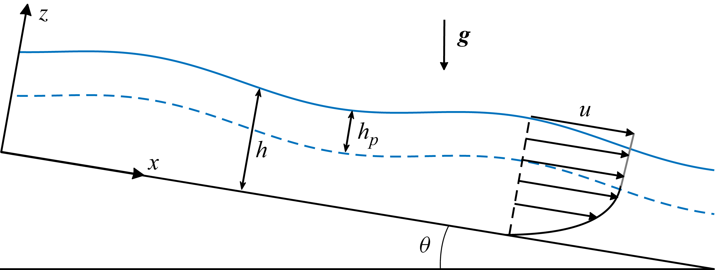
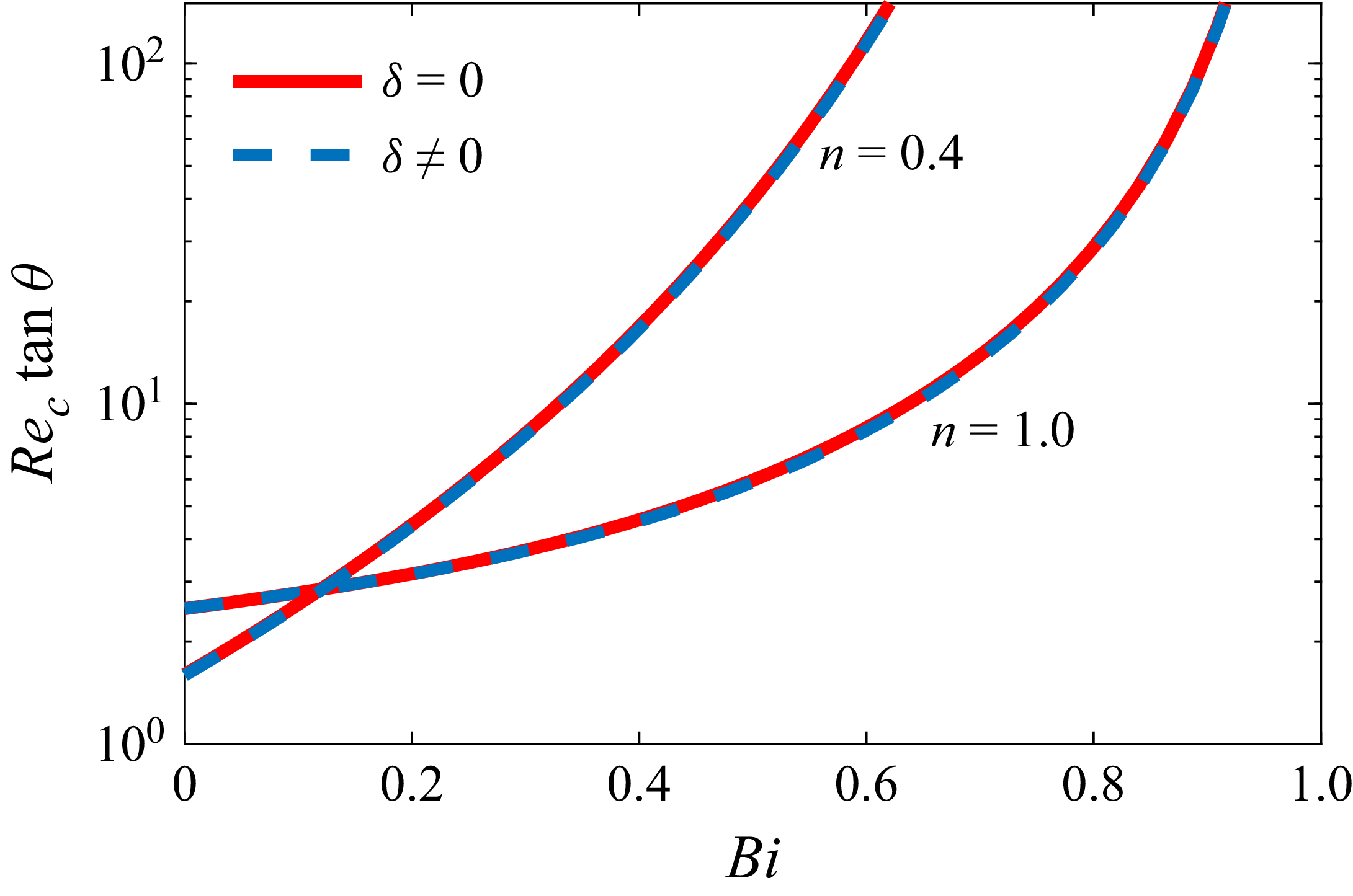


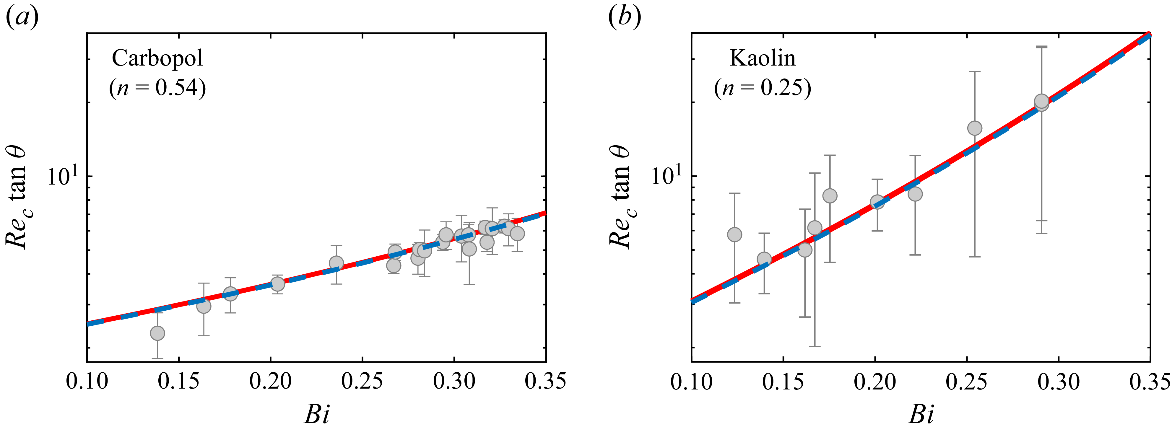


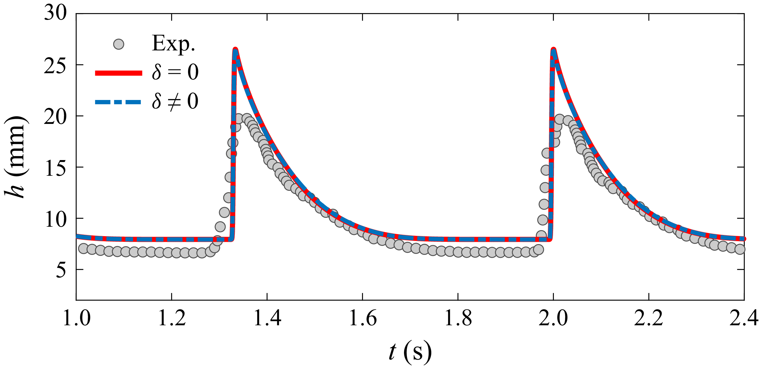


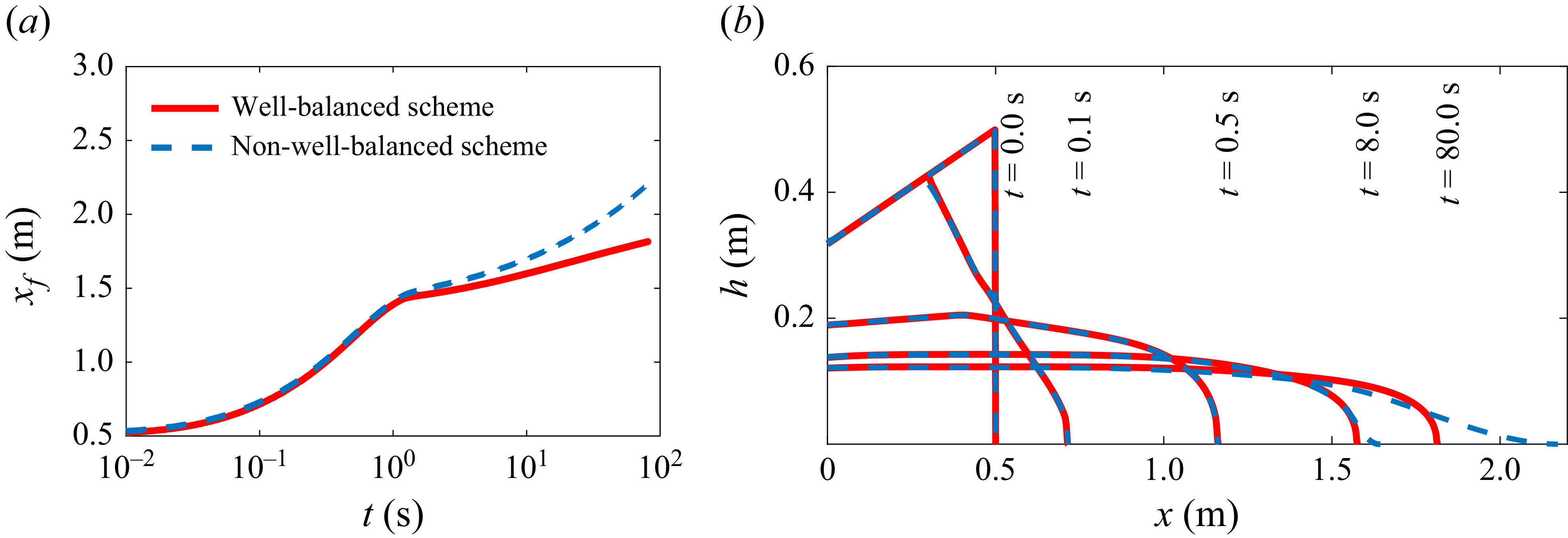


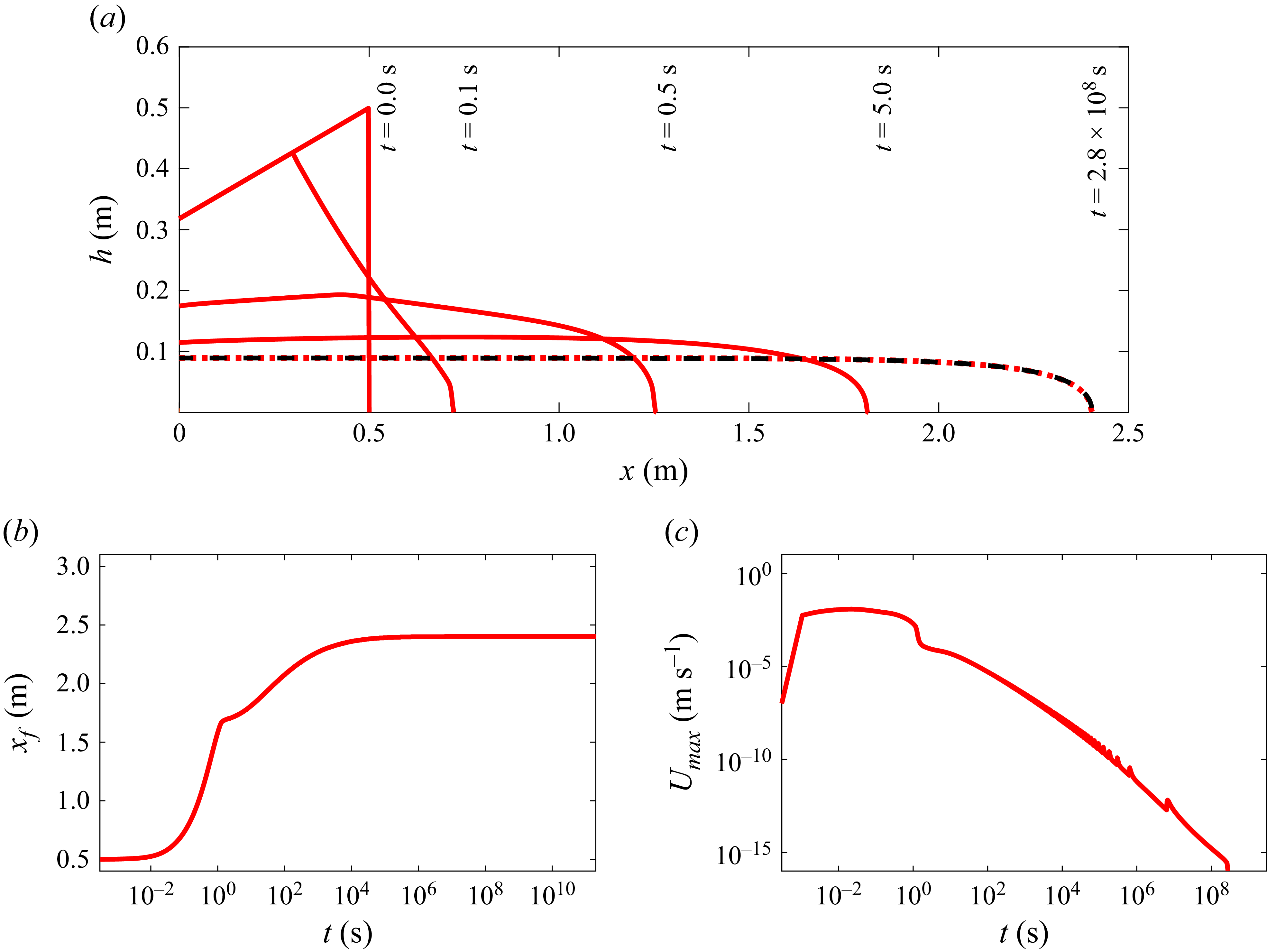


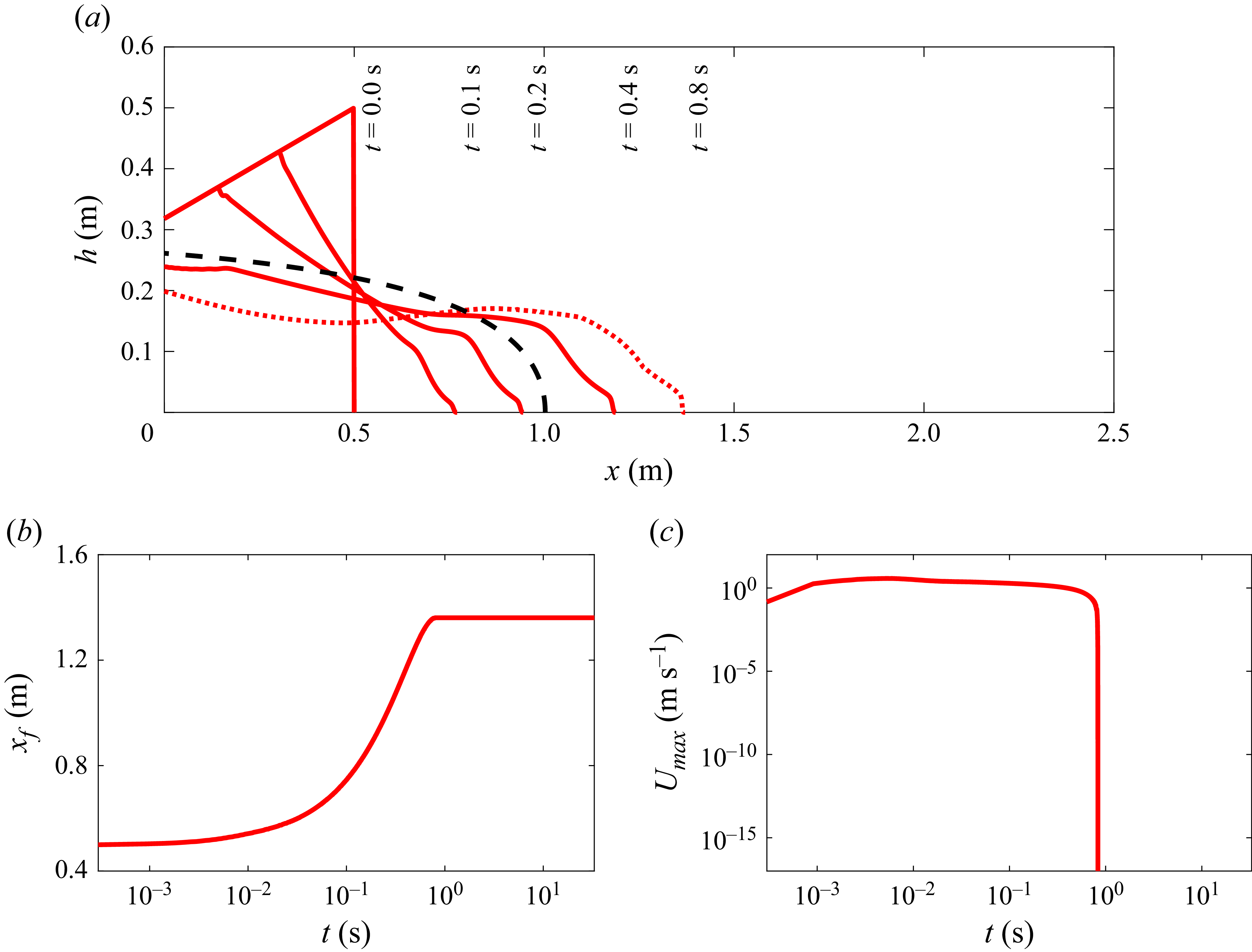





 Open access

