


1. Introduction
The stable production of arbitrarily thin fluid jets has become the ‘holy grail’ for many microfluidic applications that demand monodisperse collections of tiny droplets, bubbles, capsules and emulsions. The microjetting mode of tip streaming (Anna & Mayer Reference Anna and Mayer2006; Montanero & Gañán-Calvo Reference Montanero and Gañán-Calvo2020) has been the preferred method in most cases because it allows the formation of long fluid threads much thinner than any fluid passage of the microfluidic device. Using hydrodynamic (De Bruijn Reference De Bruijn1993) or electrohydrodynamic forces (Duft et al. Reference Duft, Achtzehn, Muller, Huber and Leisner2003), energy is gently focused into the tip of a tapering meniscus anchored to the feeding tube. In a particular region of the parameter space, the meniscus tip steadily emits a jet much thinner than the tube. The jet eventually breaks up into droplets due to the capillary instability.
In most tip streaming realizations, the kinetic energy per unit volume  $\rho _j v_j^2/2$ ( $\rho _j$ and $v_j$ are the jet's density and velocity, respectively) gained by the inner-phase fluid particle results from the work done by the external driving force on the tapering meniscus (the pressured drop applied to an outer gas current, the electric field, etc.). This work is approximately fixed when the driving force intensity is fixed (Montanero & Gañán-Calvo Reference Montanero and Gañán-Calvo2020). Therefore, the fluid particle kinetic energy is practically independent of the injected flow rate $Q_i$. This implies that the jet diameter $d_j\sim (Q_i/v_j)^{1/2}$ scales approximately as $Q_i^{1/2}$.
In principle, the jet diameter can be indefinitely reduced by lowering the injected flow rate. However, experiments and numerical simulations have shown that the flow inevitably becomes unstable at a critical value of  $Q_i$, which sets a minimum value of the jet diameter (Montanero & Gañán-Calvo Reference Montanero and Gañán-Calvo2020). For instance, the microjetting modes of gravitational jets (Rubio-Rubio, Sevilla & Gordillo Reference Rubio-Rubio, Sevilla and Gordillo2013), flow focusing (Cruz-Mazo et al. Reference Cruz-Mazo, Herrada, Gañán-Calvo and Montanero2017), confined selective withdrawal (Evangelio, Campo-Cortés & Gordillo Reference Evangelio, Campo-Cortés and Gordillo2016; López et al. Reference López, Cabezas, Montanero and Herrada2022) and electrospray (Ponce-Torres et al. Reference Ponce-Torres, Rebollo-Muñoz, Herrada, Gañán-Calvo and Montanero2018) become unstable at this well-known minimum flow rate stability limit, which prevents producing jets with arbitrarily small diameters.
A number of significant studies of the microjetting mode of tip streaming demonstrated the production of thin jets, but they did not determine the minimum flow rate stability limit. Using a double flow-focusing arrangement, Gañán-Calvo et al. (Reference Gañán-Calvo, González-Prieto, Riesco-Chueca, Herrada and Flores-Mosquera2007) produced compound fluid jets with submicrometre diameters. The transient numerical simulations of Suryo & Basaran (Reference Suryo and Basaran2006) showed the transition from jetting to microjetting (tip streaming) in the coflowing configuration when the inner-to-outer flow rate ratio decreased below a critical value. The vanishing flow rate ratio limit was not analysed in that work.
It is worth mentioning that Gañán-Calvo (Reference Gañán-Calvo2008) showed that an infinitely thin jet is stable (convectively unstable) if the interface speed exceeds a critical value, which depends on the ratio between the jet and outer medium viscosities. However, this must be regarded as a prerequisite for microjetting, which does not consider the critical instability that originates in the tapering meniscus.
Gordillo, Sevilla & Campo-Cortés (Reference Gordillo, Sevilla and Campo-Cortés2014) studied the stability of fluid jets stretched by a coflowing viscous current using a one-dimensional approach. In this approach, the outer flow field was calculated as the addition of the unperturbed flow field (i.e. that obtained if the inner fluid were not injected) plus a distribution of sources located at the axis of symmetry. The outer tube was much bigger than the inner one, therefore, the effect of confinement could be neglected. They found both oscillatory and non-oscillatory critical modes. The perturbation amplitude in the tapering cone was virtually zero in the oscillatory mode. Gordillo et al. (Reference Gordillo, Sevilla and Campo-Cortés2014) also showed the critical stabilizing effect of the capillary pressure gradient in the stretched jets.
Taylor (Reference Taylor1932, Reference Taylor1934) proposed a long-wave model to describe the flow in an axisymmetric drop submerged in a viscous uniaxial extensional flow. Using this approximation, Zhang (Reference Zhang2004) showed how the extensional flow might produce a vanishingly thin jet from the tip of a meniscus attached to a tube. A continuous transition to microjetting with an arbitrarily small flow rate (jet diameter) can occur when the imposed capillary number is decreased. As the flow rate decreases, the solution to the long-wave model tends to a universal velocity profile when the variables are appropriately scaled. However, these numerical results were based on the slender body theory, which is known to fail for conical tips (Eggers Reference Eggers2021). More importantly, the flow stability was not determined, and, therefore, the viability of this method was not demonstrated. It must be pointed out that numerical simulations usually converge to a microjetting solution even when the bifurcation point has been crossed, making the stability analysis critical.
This work examines the microjetting mode obtained when a fluid is injected at the flow rate  $Q_i$ through a tube submerged in a uniaxial extensional flow ( $-Gr/z,0,Gz$). We analyse the flow stability as $Q_i$ decreases. Our main conclusion is that infinitely thin jets can be stably produced for a sufficiently large outer viscosity, independently of the jet viscosity and the outer flow intensity $G$.
$G$.
To analyse the microjetting stability in the limit  $Q_i\to 0$, we also study the stability and breakup of a droplet in a uniaxial extensional flow with its equator pinned to an infinitely thin ring. This problem is practically the same as that described above for $Q_i=0$. The response of a suspended droplet to a linear flow has been the subject of study in numerous works. For this reason, considering the pinned droplet problem not only allows us to discuss the limit $Q_i\to 0$ of the microjetting mode but also is interesting in itself. Our analysis will show how the pinning of the droplet equator drastically affects the droplet stability and breakup.
The paper is organized as follows. In § 2, we present the governing equations and formulate the two related problems solved in this work: (i) the stability of a closed droplet pinned to the feeding capillary and deformed by the outer uniaxial extensional flow, and (ii) the stability of the microjetting mode produced when the inner disperse phase is injected across the feeding capillary at a constant flow rate. The global stability analysis and the numerical method are also briefly described in this section. The results for the closed droplet are shown in § 3, while the analysis of the microjetting mode stability is presented in § 4. In this section, we also discuss the relationship between these two problems. The paper closes with some conclusions and final remarks in § 5.
2. Governing equations
Consider a cylindrical capillary of radius  $a$ placed in a linear uniaxial extensional flow given by the equations
 \begin{equation} u^{({o})}=-Gr/2,\quad w^{({o})}=G z, \end{equation}
where  $u^{({o})}$ and $w^{({o})}$ are the radial and axial components of the velocity field, and $G$ is the flow intensity. The centre of the capillary exit is located at the origin of the cylindrical coordinate system ( $r, z$). The density and viscosity of the outer fluid are $\rho _o$ and $\mu _o$, respectively.
In the first problem analysed in this work, a droplet of volume  $V$, density $\rho _i$ and viscosity $\mu _i$ is pinned to the edge of the capillary (figure 1). The pinning condition implies that the triple contact line does not move because it remains anchored to the capillary edge. This case corresponds to a closed droplet submerged in an extensional flow with its equator pinned to an infinitely thin ring. We will refer to this problem as the case $Q_i=0$, which alludes to the fact that the inner phase does not need to be injected to sustain the steady flow in the droplet.
Sketch of the fluid domain for the closed droplet ( $Q_i=0$). The blue line is the shape of the droplet stretched by the outer flow. The interface is pinned to the sharp capillary edge, as indicated in the sketch. The dashed lines indicate the borders of the computational domain. The velocity field (2.1a,b) is prescribed at the upper and right-hand borders. The left-hand border is a symmetry plane. The lower border is a symmetry axis.

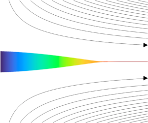
The second problem studied in this work considers the microjetting mode achieved when the inner phase is injected at the constant flow rate  $Q_i$ through the capillary (figure 2). In this case, the inner phase forms a cone-like tapering meniscus that ejects a very thin jet from its tip. The issued fluid volume is replaced by that injected across the capillary so that the system can adopt a steady flow. We will refer to this problem as the case $Q_i>0$.
Sketch of the fluid domain for the microjetting mode ( $Q_i>0$). The blue line is the interface location. The interface is pinned to the sharp capillary edge, as indicated in the sketch. The dashed lines indicate the borders of the computational domain. The velocity field (2.1a,b) is prescribed at the upper and right-hand borders. The left-hand border is a symmetry plane. The lower border is a symmetry axis. The parabolic velocity profile is prescribed at a distance $L_0$ from the exit of the feeding capillary.

Hereafter, all the variables are made dimensionless with the characteristic length  $a$, velocity $\sigma /\mu _o$, time $\mu _o a/\sigma$ and stress $\sigma /a$, where $\sigma$ is the surface tension. In this section, we present the equations in cylindrical coordinates. This coordinate system is used to analyse the stability of the microjetting mode. The equations in intrinsic coordinates for the closed droplet can be found elsewhere (Herrada, Yu & Stone Reference Herrada, Yu and Stone2023).
The dimensionless, axisymmetric, incompressible Navier–Stokes equations for the velocity and pressure fields are
 $$\begin{gather} [ru^{(k)}]_r+rw^{(k)}_z = 0, \end{gather}$$
 $$\begin{gather}(\lambda^2)^{\delta_{ik}} {Re}_k[u^{(k)}_t + u^{(k)} u^{(k)}_r+ w^{(k)} u^{(k)}_z] =-p^{(k)}_r+\lambda^{\delta_{ik}}[ u^{(k)}_{rr}+(u^{(k)}/r)_r+u^{(k)}_{zz}], \end{gather}$$
 $$\begin{gather}(\lambda^2)^{\delta_{ik}} {Re}_k[w^{(k)}_t + u^{(k)} w^{(k)}_r+ w^{(k)}w^{(k)}_z] =- p^{(k)}_z+\lambda^{\delta_{ik}}[w^{(k)}_{rr}+w^{(k)}_r/r+w^{(k)}_{zz}], \end{gather}$$
where  $u^{(k)}$ ( $w^{(k)}$) is the radial (axial) velocity component, $p^{(k)}$ is the pressure field, $Re_k=\rho _k \sigma a/\mu _k^2$ is the Reynolds number (the inverse of the Ohnesorge number) of phase $k, \lambda =\mu _i/\mu _o$ is the viscosity ratio and $\delta _{ij}$ is the Kronecker delta. In the above equations and henceforth, the subscripts and superscripts $k=i$ and $o$ refer to the inner and outer phases, respectively, and the subscripts $t, r$ and $z$ denote the partial derivatives with respect to the corresponding variables. The action of the gravitational field has been neglected due to the smallness of the fluid configuration.
The kinematic compatibility condition at the interface reads
 \begin{equation} F_t+F_z w^{(i)}-u^{(i)}=0,\end{equation}
where  $r=F(z,t)$ is the distance of an interface element to the symmetry axis $z$. We consider the continuity of the velocity field and tangential stress at the interface, as well as the normal stress jump due to the capillary pressure,
 \begin{equation} \|{\boldsymbol v}^{(k)}\|={\boldsymbol 0}, \quad \|\tau^{(k)}_t\|=0,\quad \|\tau^{(k)}_n\|=\kappa, \end{equation}
where  $\|A^{(k)}\|$ denotes the difference $A^{(i)}-A^{(o)}$ between the values taken by the quantity $A$ on the two sides of the interface, $\boldsymbol {v}^{(k)}(r,z;t), \tau ^{(k)}_t$ and $\tau ^{(k)}_n$ represent the velocity field and tangential and normal stress, respectively, and $\kappa$ is the local mean curvature.
The triple contact line anchorage condition,  $F=1$, is set at the capillary edge (the triple contact line is pinned to the capillary edge). We impose the velocity field $u^{(o)}=-Cr/2$ and $w^{(o)}=Cz$ (see (2.1a,b)) at the two boundaries of the computational domain indicated in figures 1 and 2, where $C=Ga\mu _o/\sigma$ is the capillary number. The outer uniaxial extensional flow is symmetric with respect to the plane $z=0$; i.e. ${\rm d} u^{(o)}/{\rm d} z=w^{(o)}=0$. The lower boundary corresponds to a symmetry axis.
The above equations and boundary conditions apply to the two problems  $Q_i=0$ and $Q_i>0$ considered in this work. In the case $Q_i=0$, the flow in the droplet is also symmetric with respect to the plane $z=0$; i.e. ${\rm d} u^{(i)}/{\rm d} z=w^{(i)}=0$ at $z=0$ (figure 1). In this way, we simulate one of the two halves of a droplet whose equator is pinned to an infinitely thin ring. This is not strictly equivalent to imposing $Q_i=0$ at the feeding capillary exit. However, it is expected to have negligible influence on the linear stability of the microjetting realizations analysed in this paper, which is essentially determined by the flow in the meniscus–jet transition region.
For  $Q_i=0$, the droplet volume
 \begin{equation} V=2{\rm \pi} \int_0^{\varLambda} F^2\, {\rm d} z, \end{equation}
is prescribed to calculate the base flow in the linear stability analysis and as an initial condition in the transient simulations. Here,  $\varLambda$ is the length of half the drop ( $F(\varLambda )=0$).
For  $Q_i>0$, the symmetry plane condition is only considered on the left-hand side of the outer computational domain, as indicated in figure 2. The parabolic velocity profile corresponding to the dimensionless flow rate $Q=Q_i/({\rm \pi} a^2 \sigma /\mu _o)$ is imposed inside the feeding capillary at a distance $L_0$ from its exit ( $L_0=5$ in the simulations unless otherwise stated). Finally, the outflow boundary conditions $F_z=u^{(i)}_z=w^{(i)}_z=0$ are prescribed in the jet outlet cross-section.
Different sets of parameters characterize the problems for  $Q=0$ and $Q>0$. For $Q=0$, the problem is formulated in terms of the dimensionless numbers $\{Re_i, Re_o, \lambda, C, V\}$. For a fixed value of $L_0$, the problem with $Q>0$ is characterized by the parameters $\{Re_i, Re_o, \lambda, C, Q\}$, which reduce to $\{\lambda, C, Q\}$ when inertia is neglected. We will consider this approximation in most of our analysis.
The viscosity ratio and Reynolds numbers are defined in terms of the material properties and the capillary radius, which allows fixing their values in an experimental run in which the strain rate (the capillary number) and injected flow rate are changed. These two variables are the experimental operational parameters.
To calculate the linear global modes of the steady solution, we assume the temporal dependence
 \begin{equation} U=U_0+\delta U\, {\rm e}^{-{\rm i}\omega t}+\text{c.c.} \quad (|\delta U|\ll |U|), \end{equation}
where  $U$ represents any unknowns of the problem, and $U_0$ and $\delta U$ stand for the corresponding base flow (steady) solution and the spatial dependence of the eigenmode, respectively.
For  $Q=0$, the interface location is defined in terms of intrinsic coordinates. In this case, we assume the temporal dependence
 \begin{equation} (r_s,z_s)=(r_{s0},z_{s0})+(\delta r_s,\delta z_s)\, {\rm e}^{-{\rm i}\omega t}+\text{c.c.} \quad (|\delta r_s|\ll r_{s0}, |\delta z_s|\ll z_{s0}), \end{equation}
where  $(r_{s0},z_{s0})$ is the droplet shape in the base flow, and $(\delta r_s,\delta z_s)$ is the perturbation. For $Q>0$, we assume the temporal dependence for the interface location
 \begin{equation} F=F_0+\delta F\, {\rm e}^{-{\rm i}\omega t}+\text{c.c.} \quad (|\delta F|\ll F_0), \end{equation}
where  $F_0$ denotes the interface position in the base flow, and $\delta F$ is the perturbation. In the above equations, $\omega =\omega _r+{\rm i}\omega _i$ is the eigenfrequency characterizing the perturbation evolution. If the growth rate $\omega _i^*$ of the dominant mode (i.e. that with the largest $\omega _i$) is positive, then the base flow is asymptotically unstable under small-amplitude perturbations (Theofilis Reference Theofilis2011).
We used a boundary-fitted spectral method (Herrada & Montanero Reference Herrada and Montanero2016) to solve the theoretical model described above. Here, we summarize the main characteristics of this method. The inner and outer fluid domains are mapped onto two quadrangular domains through non-singular mapping. A quasielliptic transformation (Dimakopoulos & Tsamopoulos Reference Dimakopoulos and Tsamopoulos2003) is applied in the outer bath. All the derivatives appearing in the governing equations are expressed in terms of the spatial coordinates resulting from the mapping. These equations are discretized in the mapped radial direction with Chebyshev spectral collocation points (Khorrami, Malik & Ash Reference Khorrami, Malik and Ash1989). We use fourth-order finite differences with equally spaced points to discretize the mapped axial direction for  $Q>0$. Details of the discretization used with intrinsic coordinates for $Q=0$ can be found elsewhere (Herrada et al. Reference Herrada, Yu and Stone2023). The MATLAB eigs function is applied to find the eigenfrequencies around a reference value $\omega _0$. This process is repeated for several values of $\omega _0$.
We conduct transient (direct) numerical simulations for both  $Q=0$ and $Q>0$. These simulations allow us to determine the breakup mode adopted by the closed droplet for supercritical conditions. They also enable us to study the response of the microjetting mode to an initial perturbation. Second-order backward finite differences are used to discretize the time domain. For $Q=0$, the time step is adapted in the course of the simulation according to the formula $\Delta t=\Delta t_0/v_{tip}$, where $\Delta t_0$ is the time step at the initial instant, and $v_{tip}$ is the droplet tip velocity. For $Q>0$, the time step is constant. The time-dependent mapping of the physical domain does not allow the algorithm to go beyond the interface pinch-off. Therefore, the evolution of the emitted droplet cannot be analysed using the present code.
The numerical method for studying the stability of the microjetting mode has been extensively used and validated from comparison with experiments (Cruz-Mazo et al. Reference Cruz-Mazo, Herrada, Gañán-Calvo and Montanero2017; Ponce-Torres et al. Reference Ponce-Torres, Rebollo-Muñoz, Herrada, Gañán-Calvo and Montanero2018; López et al. Reference López, Cabezas, Montanero and Herrada2022). The adaptation of this method to the stability analysis of a closed droplet was validated by Herrada et al. (Reference Herrada, Ponce-Torres, Rubio, Eggers and Montanero2022) from comparison with other numerical approaches and asymptotic analyses.
The next two sections present the results for the two problems described above: the closed droplet ( $Q=0$) and the microjetting mode ( $Q>0$). First, we analyse the deformation and stability of a closed droplet pinned to the capillary edge. As shown below, the solution to this problem is intimately related to that of the microjetting mode in the limit $Q\to 0$. We also show the fundamental differences between the results previously obtained for an unpinned droplet and those for the pinned case.
In § 4, we focus on the most interesting case of the microjetting mode adopted by the system for  $Q>0$. We determine the stability limits and discuss the system behaviour in the limit $Q\to 0$. We establish the connection between the behaviour of a closed droplet ( $Q=0$) and microjetting for $Q\to 0$. Transient simulations are conducted to relate the global stability analysis to the system behaviour close to the stability limit. We discuss the mechanisms that can explain the stability of the microjetting regime for arbitrarily small values of $Q$. The effect of inertia is shown in the last part of this section.
3. Results for  $Q=0$
$Q=0$

We start this section by summarizing previous results for the classical problem of an unpinned droplet suspended in an extensional uniaxial flow. The viscous force exerted by the outer fluid deforms the droplet, which adopts an oblate shape. The magnitude of this deformation increases with the capillary number. The droplet apex sharpens in the direction of the outer flow as  $\lambda$ decreases. The viscosity force drives a steady recirculation flow inside the droplet (Herrada et al. Reference Herrada, Ponce-Torres, Rubio, Eggers and Montanero2022).
For sufficiently large values of the capillary number, the flow becomes unstable at a saddle-node bifurcation (Eggers & Courrech du Pont Reference Eggers and Courrech du Pont2009). This bifurcation corresponds to a turning point when the droplet deformation  $D=(\hat {a}-\hat {b})/(\hat {a}+\hat {b})$ ( $\hat {a}$ and $\hat {b}$ are the half-length and half-breadth of the cross-sectional shape, respectively) is plotted against the capillary number (Taylor Reference Taylor1964; Acrivos & Lo Reference Acrivos and Lo1978). As shown below, both the real and imaginary parts of the critical eigenfrequency vanish at the bifurcation. The critical non-oscillatory eigenmode produces a thinning of the droplet equator (Herrada et al. Reference Herrada, Ponce-Torres, Rubio, Eggers and Montanero2022). This thinning increases in magnitude until the interface pinches, giving rise to two droplets equal in size (the so-called central pinching mode or end-pinching mechanism (Gallino, Schneider & Gallaire Reference Gallino, Schneider and Gallaire2018)). The Taylor (Reference Taylor1964) slender body theory predicts the critical capillary number $0.0745 \lambda ^{-1/6}$ for $\lambda \to 0$. For $\lambda =0.0125$, this theory predicts the value 0.155, while the solution of the full hydrodynamic equations leads to the value 0.242. Thus, while slender body theory predicts the correct type of transition, it only yields semiquantitative results, and full numerical simulations are needed.
The simulations conducted in this work for  $Q=0$ correspond to the problem described above except for a fundamental difference: the droplet equator is a triple contact line pinned to the feeding capillary edge in the present study. Figure 3 shows the droplet deformation $D$ and growth rate of the dominant mode, $\omega _i^*$, versus the capillary number $C$ for a pinned droplet. For the sake of comparison, we also show the results corresponding to the unpinned droplet (Herrada et al. Reference Herrada, Ponce-Torres, Rubio, Eggers and Montanero2022). In both cases, the solution reaches a saddle-node bifurcation, which corresponds to a turning point of the curve $D(C)$. The solution for the unstable branch beyond the turning point is calculated by imposing the droplet interface length and calculating the corresponding capillary number (Herrada et al. Reference Herrada, Yu and Stone2023). The pinning condition suppresses the central pinching mode, considerably increasing the critical capillary number.
(a) Droplet deformation  $D$ and (b) growth rate of the dominant mode, $\omega _i^*$, versus the capillary number $C$. The results were calculated as a function of the capillary number $C$ for $Re_i= Re_o=0, \lambda =0.1$ and $V=4{\rm \pi} /3$. The circles (squares) correspond to the pinned (unpinned) droplet. The dotted lines indicate the critical capillary numbers. The solid symbols show the crossover of two modes.

Figure 4 shows the spectrum of eigenvalues around  $\omega _0=0.1$ for two solutions next to the saddle-node bifurcation. At marginal stability, both the frequency and damping rate (the growth rate with the sign reversed) of the dominant eigenvalue vanish. This means that the flow becomes unstable under stationary (non-oscillatory) linear perturbations.
Eigenvalues around  $\omega _0=0.1$ for a pinned droplet with $D=0.32$ (red symbols) and 0.33 (black symbols). In addition, $Re_i= Re_o=0, \lambda =0.1, C=0.3$ and $V=4{\rm \pi} /3$.

The interface displacement due to the growth of the critical eigenmode at the quasimarginally stable is analysed in figure 5. This displacement corresponds to the interface deformation at the initial (linear) phase of the droplet breakup. We compare the results with those obtained for the unpinned droplet at the corresponding marginal stability (Herrada et al. Reference Herrada, Ponce-Torres, Rubio, Eggers and Montanero2022). In this case, the perturbation affects most of the interface, not only the droplet tip. The nonlinear growth of this perturbation gives rise to the central pinching mode (figure 6). When the interface is pinned, the mode containing a uniform extension (and thus a shrinking equator) is suppressed, and the drop is no longer pulled apart. Instead, the critical perturbation is localized in the droplet tip (figure 5). The growth of this perturbation gives rise to microdripping (figure 7) instead of the central pinching mode.
Droplet shape in the base flow,  $(r_{s0},z_{s0})$ (shaded area), and interface displacement due to the critical linear eigenmode, $(r_s,z_s)=(r_{s0},z_{s0})+\phi ({Re}[\delta r_s], {Re}[\delta z_s])$ (dashed lines), for $\lambda =0.1$ and $C=0.17$ (a), $\lambda =0.1$ and $C=0.30$ (b), $\lambda =0.0125$ and $C=0.25$ (c) and $\lambda =0.0125$ and $C=0.55$ (d). In the two cases, $Re_i= Re_o=0$, and $V=4{\rm \pi} /3$. The value of the arbitrary constant $\phi$ in the linear analysis has been chosen to appreciate the interface deformation.

Shape of an unpinned droplet suspended in an extensional uniaxial flow at different instants for  $Re_i= Re_o=0, \lambda =0.0125, C=0.26$ and $V=4{\rm \pi} /3$. The colour scale indicates the magnitude of the interface velocity relative to the magnitude of the imposed external flow at that point. The inner phase moves towards the droplet apex. Since the droplet equator is not pinned, the equator interface radius decreases until the interface pinches.

Droplet shape right before the breakup for  $Re_i= Re_o=0$ and $V=4{\rm \pi} /3$. The images correspond to $\lambda =0.1$ (a) and $\lambda =0.0125$ (b), and their respective critical capillary numbers $C=0.31$ and 0.56. The colour scale indicates the magnitude of the interface velocity relative to the magnitude of the imposed external flow at that point. The triple contact line is pinned to the capillary edge.

The critical capillary number increases as  $\lambda$ decreases. Consequently, the droplet stretches at the stability limit, the outer velocity around the droplet tip considerably increases and the tip curvature grows. For small values of $\lambda$, the microdripping mode produces tiny droplets much smaller than the mother drop (figure 7). The effect of the contact line pinning is somewhat similar to covering the droplet with a surfactant monolayer (Eggleton, Tsai & Stebe Reference Eggleton, Tsai and Stebe2001; Herrada et al. Reference Herrada, Ponce-Torres, Rubio, Eggers and Montanero2022). This effect has also been considered in other microfluidic configurations (Dewandre et al. Reference Dewandre, Rivero-Rodriguez, Vitry, Sobac and Scheid2020).
4. Results for $Q>0$

We now focus on the more interesting case  $Q>0$, where a fluid is injected at a constant rate $Q$ through the feeding capillary placed in the extensional flow. As a result, a steady state can be maintained while continuously producing microdroplets. We first consider flows dominated by viscosity ( $Re_i= Re_o=0$), characterized only by the viscosity ratio $\lambda$, the capillary number $C$ and the injected flow rate $Q$. The effect of inertia will be analysed at the end of this section.
4.1. Stability limit
Figure 8 shows the evolution of the spectrum of eigenvalues when the capillary number decreases below the critical value. In all the cases for  $Q>0$ considered in this work, $\omega _r^*\neq 0$, which means that the flow becomes unstable due to an oscillatory supercritical Hopf bifurcation linked to the presence of the jet. The jet convects capillary modes, which translates into an oscillatory behaviour in the Eulerian frame of reference. In fact, this oscillatory instability has been observed in the microjetting mode of practically all the configurations analysed so far (Montanero & Gañán-Calvo Reference Montanero and Gañán-Calvo2020). Non-oscillatory critical modes are expected when the instability is confined in a region of the fluid domain. This is not the behaviour observed in our simulations, as seen in figure 9. Instead, the unstable mode extends significantly to the jet. In the case of the smaller $\lambda$, the unstable mode is concentrated mostly in the jet. Gordillo et al. (Reference Gordillo, Sevilla and Campo-Cortés2014) found both oscillatory and non-oscillatory critical modes in the coflow configuration. However, they claimed that the oscillatory instability dominates over the steady one within the ranges of viscosity and flow rate ratios explored in their analysis.
Eigenvalues around  $\omega _0=0.5$ for $Re_i= Re_o=0, \lambda =0.0125, Q=0.00126$ and $C=0.131$ (black circles) and 0.132 (red circles).

Interface contour (red solid line) and magnitude of the interface perturbation,  $|\delta F|$ (black dotted line), for ( $\lambda =0.1, C=0.425, Q=0.00126$) (a) and ( $\lambda =0.0125, C=0.130, Q=0.00126$) (b). The magnitude of the interface perturbation has been normalized with its maximum value $|\delta F|_{max}$. In the two cases, $Re_i= Re_o=0$.

The magnitude of the critical interface perturbation is plotted in figure 9 for  $\lambda =0.1$ and 0.0125, and the same flow rate $Q=0.00126$. For $\lambda =0.1$, the meniscus contour is perturbed in front of its tip, while $|\delta F| \simeq 0$ in the cone for $\lambda =0.0125$. The result for $\lambda =0.0125$ is similar to that obtained in the coflow configuration (Gordillo et al. Reference Gordillo, Sevilla and Campo-Cortés2014). The growth of the interface oscillation eventually produces the interface pinching (see § 4.3), and the system evolves from steady microjetting towards some type of dripping.
Figure 10(a) shows the stability map in the parameter plane ( $C, Q$) for several values of the viscosity ratio $\lambda$. We could not conduct simulations for $Q\lesssim 10^{-4}$ because of the sharp increase in the computing time caused by the much smaller flow scales generated as $Q$ decreases. The symbols correspond to marginally stable cases for which $\omega _i^*=0$.
(a) Stability map for viscosity-dominated flow ( $Re_i= Re_o=0$). The symbols correspond to marginally stable ( $\omega _i^*=0$) microjetting realizations. (b) Fitting (4.1) to the stability limits shown in graph (a). The solid lines are splines through the simulation data, and the dashed lines correspond to (4.1) with $Q^*=0.0314, C^*=0.142, a_1=6.71, \lambda ^*=0.0161$ and $c_3=0.015$.

The results reveal an interesting dependence of the critical capillary number on  $\lambda$ for a fixed flow rate. All the stability curves approximately intersect at $Q=Q^*\simeq 0.031$ and $C=C^*\simeq 0.15$. For $Q\gtrsim 0.031$, the critical capillary number decreases as $\lambda$ increases, while the opposite occurs for $Q\lesssim 0.031$. We conclude that the inner viscosity stabilizes the flow for $Q\gtrsim 0.031$ but destabilizes it for sufficiently small flow rates. Increasing the capillary number always stabilizes the jet, which shows the stabilizing effect of the outer flow intensity.
Two types of asymptotic behaviour of the stability limit  $Q(C)$ can be observed in figure 10(a) as $Q\to 0$. For $\lambda \geq 0.02, Q\sim C^{\alpha }$ with $\alpha <0$, which implies that, for any value of $C$, there is a finite value of $Q$ below which the steady flow becomes unstable. This is the expected behaviour because it corresponds to what has been observed in all tip streaming configurations (Montanero & Gañán-Calvo Reference Montanero and Gañán-Calvo2020). In contrast, $Q(C)$ seems to approach a vertical asymptote $C=0.131$ for $\lambda =0.0125$. This means that the flow remains stable for infinitely small values of $Q$ provided that $C\geq 0.131$. This result constitutes the central finding of this work.
The above conclusion has obvious practical consequences. As explained in the Introduction, the jet diameter scales as  $Q^{1/2}$ at a fixed distance from the feeding capillary, and hence fluid jets with vanishing diameters can be steadily emitted as $Q\to 0$. As the outer viscosity increases at a fixed jet viscosity and outer flow intensity, $\lambda$ decreases and $C$ increases. For $\lambda <\lambda ^*$ and $C$ sufficiently large, one is in the stable regime of figure 10(a), and arbitrarily thin jets can be realized. We conclude that jets with vanishing diameters can be produced for a large enough outer viscosity, independently of the jet viscosity and outer flow intensity. For a fixed outer viscosity, infinitely thin jets can also be produced if the jet viscosity (the viscosity ratio $\lambda$) is sufficiently small and the flow intensity (the capillary number $C$) is large enough.
As mentioned above, there is a critical flow rate  $Q^*\simeq 0.031$ for which the critical number $C^*\simeq 0.15$ is practically independent of $\lambda$. In order to bring out the universal character of the behaviour change that takes place as $\lambda$ is varied, we perform an expansion around the invariant point $(Q^*,C^*)$, where $Q^*=0.031$ is a critical flow rate, and $C^*=0.15$ is the corresponding capillary number. This suggests introducing the relative parameters $\bar {Q}=\log _{10}Q-\log _{10}Q^*$ and $\bar {C}=\log _{10}C-\log _{10}C^*$, where the logarithmic scale was chosen for convenience. Note that in figure 10(b), we have written $\bar {C}$ as a function of $\bar {Q}$ to write all curves as graphs.
For a critical viscosity ratio  $\lambda = \lambda ^*$, the above transition implies $\partial \bar {C}/\partial \bar {Q} = 0$ at $\bar {C}=\bar {Q}=0$, and thus a linear description $\bar {C}=a_1(\lambda -\lambda ^*)\bar {Q}$ in the immediate neighbourhood of the bifurcation. Expanding to higher order in powers of $\bar {Q}$, a quadratic term would result in a local maximum for both $\lambda <\lambda ^*$ and $\lambda >\lambda ^*$, and thus would not be describing a transition. This suggests retaining a cubic term, resulting in the local normal form
 \begin{equation} \bar{C}=a_1(\lambda-\lambda^*)\bar{Q}-c_3\bar{Q}^3. \end{equation}
This expresses concisely the transition from  $\lambda > \lambda ^*$, for which instability always occurs for sufficiently small $Q$, to the unconditional jetting region $\lambda < \lambda ^*$, for which there is a local maximum of the $\bar {C}(\bar {Q})$ curve.
The simple, universal form of the description (4.1) could be a starting point for a future, more systematic bifurcation analysis based on the equations of motion. In addition, on a purely descriptive level, fitting (4.1) to the numerical simulations leads to  $Q^*=0.0314, C^*=0.142, a_1=6.71, \lambda ^*=0.0161$ and $c_3=0.015$. As seen in figure 10(b), this results in a good quantitative description of the entire family of curves with a single set of parameters.
4.2. Comparison with the case $Q=0$

We now show that for small  $\lambda$, microjetting solutions have a counterpart in the pinned drop at $Q=0$, such that the meniscus shape at finite $Q$ closely resembles the shape of the drop. To this end, we analyse the case $\lambda =0.0125$ in more detail in figure 11. This figure compares the critical capillary number $C_c(Q)$ for microjetting with the value $C_{c0}$ obtained for a pinned droplet ( $Q=0$) (see § 3) with the same volume as that of the microjetting meniscus (red circles in figure 11). The meniscus volume is calculated as that delimited by the end of the feeding capillary and the stagnation point in front of the jet. This volume hardly changes for $\lambda =0.0125$ and $Q<0.05$. For this reason, $C_{c0}$ is practically constant in all the cases considered. As explained above, microjetting becomes unstable for $C< C_{c}$, while the droplet becomes unstable for $C>C_{c0}$.
(a) Critical capillary number  $C_c$ as a function of the flow rate $Q$ for viscosity-dominated flow ( $Re_i= Re_o=0$) and $\lambda =0.0125$ (blue triangles). The red circles indicate the critical capillary $C_{c0}$ for the onset of instability for a droplet with the same volume as that of the meniscus of the corresponding microjetting realization, as indicated by the arrows. (b) Sketch of a closed droplet and its microjetting counterpart.

In all the cases considered in figure 11,  $C_{c0}< C_c(Q)$. This can be interpreted as follows. Consider a pinned drop of a given (arbitrary) volume submerged in an extensional flow characterized by the capillary number $C$. At the critical capillary number $C=C_{c0}$, the drop destabilizes and ejects a tiny droplet. However, the capillary number is not large enough to maintain the liquid ejection (i.e. to produce stable microjetting) even if the ejected volume were replaced through the capillary. This occurs because $C_{c0}$ is lower than the microjetting stability threshold $C_c(Q)$. Therefore, the steady microjetting mode cannot be established.
Suppose the capillary number is further increased to  $C=C_c(Q)$, and the disperse phase is injected at the flow rate $Q$. Then, a marginally stable microjetting realization would be produced with a meniscus volume equal to that of the pinned drop. The meniscus–jet transition region becomes vanishing small as $Q\to 0$. Therefore, it is natural to hypothesize that the additional stress in the jet does not contribute to changing the meniscus shape (figure 11b). In this sense, each marginally stable pinned drop has its marginally stable ‘microjetting counterpart’.
Neither the drop nor its microjetting counterpart is stable in the interval  $C_{c0}< C< C_c(Q)$. This interval is expected to correspond to some type of dripping. The interval $C_{c0}< C< C_c(Q)$ decreases in size as $Q$ decreases because the size of the critical cone–jet transition region (the region marked with a circle in figure 11b) decreases as $Q$ decreases. We calculated the oscillation frequency $\omega _r^*$ of the critical eigenmode for $Q>0$ and verified that $\omega _r^*\to 0$ for $Q\to 0$. However, this oscillatory Hopf bifurcation becomes a non-oscillatory saddle-node bifurcation ( $\omega _r^*=0$) only at $Q=0$ due to the system ‘discontinuous’ topological change from jetting to a closed droplet at $Q=0$.
The transition from the oscillatory Hopf bifurcation for  $Q>0$ to the non-oscillatory saddle-node bifurcation for $Q=0$ has nothing to do with the symmetry plane imposed at $z=0$ for $Q=0$. A turning point also arises if one solves the problem $Q=0$ using a feeding capillary with zero flow rate.
The flow in the meniscus of the microjetting mode approaches that of the corresponding closed droplet as  $Q\to 0$ only for a sufficiently small viscosity ratio. For this reason, $C_c(Q)$ for $Q\to 0$ approximately equals $C_{c0}$ for $\lambda =0.0125$ (figure 11) but not for $\lambda =0.1$.
4.3. Transient simulations close to the stability limit
This subsection analyses the temporal evolution of a small perturbation introduced into a base flow to interpret correctly our linear stability analysis in terms of its physical outcome. The perturbation consists of the deformation of the free surface (the velocity and pressure fields are not perturbed) at  $t=0$ given by the function
 \begin{equation} F(z,0)-F_0(z)=\beta\, {\rm e}^{-(z-z_0)^2/\Delta z^2}, \end{equation}
where  $\beta$ indicates the maximum deformation, while $z_0$ and $\Delta z$ are the impulse location and width, respectively. A small amplitude ( $\beta =0.001$) deformation is introduced next to the feeding capillary ( $z_0=0.5$) with a small width ( $\Delta z=0.5$ while the meniscus length is greater than 10).
Figure 12 shows the evolution of the free surface displacement,  $F(z,t)-F_0(z)$, at the meniscus tip, as indicated in the figure. The parameter conditions correspond to a stable flow close to the stability limit. The perturbation (4.2) triggers a train of capillary waves that propagate downstream, producing a significant oscillation of the interface position in the meniscus tip. For sufficiently large $t$, the oscillation amplitude is sufficiently small for the nonlinear terms in the capillary pressure to become negligible. In addition, the contribution of subdominant eigenmodes becomes negligible, and the dominant mode essentially governs the system's linear dynamics. The comparison with the prediction
 \begin{equation} F-F_0=a_0\, {\rm e}^{\omega_i (t-t_0)}\cos[\omega_r(t-t_0)], \end{equation}
of the global stability analysis shows excellent agreement (figure 12). Here,  $a_0$ and $t_0$ are fitting parameters, and $\omega _i$ and $\omega _r$ are the damping rate and frequency of the dominant mode. The interface deformation at $t=200.1$ and 216.1 is shown in figure 13. The comparison with the deformation
 \begin{equation} F-F_0= {Re}[\delta F\, {\rm e}^{-{\rm i}\omega (t-t_0)}], \end{equation}
caused by the dominant mode shows remarkable agreement as well. Here,  $\delta F$ and $\omega =\omega _r+{\rm i}\omega _i$ are the deformation amplitude and eigenfrequency of the dominant mode, respectively.
Evolution of the free surface displacement,  $F(z,t)-F_0(z)$, at the meniscus tip ( $z=10.19, F_0(z)=0.0174$) calculated from the transient simulation for $Re_i= Re_o=0, \lambda =0.0125, C=0.135$ and $Q=0.00126$ (solid line). The dashed line is the global stability analysis's prediction (4.3) ( $a_0=0.019, t_0=7.1, \omega _i=-0.011$ and $\omega _r=0.165$). The arrow in the inset shows the analysed interface point.

Free surface displacement,  $F(z,t)-F_0(z)$, at $t=200.1$ (blue solid line) and 216.1 (red solid line) calculated from the transient simulation for $Re_i= Re_o=0, \lambda =0.0125, C=0.135$ and $Q=0.00126$. The dashed lines are the deformation (4.4) corresponding to the dominant mode ( $t_0=7.1$ and $\omega =0.165-0.011i$).

Figure 14 shows the evolution of the free surface displacement  $F(z,t)-F_0(z)$ at the meniscus tip for parameter conditions corresponding to an unstable flow close to the stability limit. The interface deformation grows while oscillating until the interface pinches. The interface pinches at $z=9.6$, close to the point $z=10.19$ analysed in figure 14. In both the stable (figure 12) and unstable (figure 14) flows, the oscillation amplitude is much greater than that of the perturbation (4.2) introduced at the initial instant next to the capillary. Therefore, the tapering meniscus amplifies that initial perturbation in the two cases. However, this amplification is much more intense in the unstable flow (figure 14). The oscillation amplitude measured in terms of the unperturbed interface radius $F_0$ sharply increases at the critical cone–jet transition region. The nonlinear terms in the capillary pressure and the interaction among modes are expected to be relevant over the oscillations observed in figure 14 because the amplitude is commensurate with $F_0$ (e.g. $F_0=0.0188$ at $z=10.19$). Therefore, the linear global stability analysis cannot accurately predict the interface evolution leading to the interface breakup.
Evolution of the free surface displacement  $F(z,t)-F_0(z)$ at three locations calculated from the transient simulation for $Re_i= Re_o=0, \lambda =0.0125, C=0.128$ and $Q=0.00126$. The arrows in the inset show the analysed interface points.

4.4. Meniscus shape and recirculation cells
The dominant flow feature inside the conical meniscus consists of two recirculation cells. By investigating the coupling of these cells with the flow inside the injection tube, we are able to extract a mechanism for instability. As explained above, the viscosity ratio  $\lambda$ essentially determines the fate of the microjetting mode as the flow rate decreases. In the limit $Q\to 0$, the microjetting mode remains stable for sufficiently small values of $\lambda$ and destabilizes otherwise. Figure 15 shows how the tapering meniscus shape changes when the flow rate is reduced by a factor of 100. For $\lambda =0.1$, the entire meniscus shrinks. Conversely, most of the cone keeps the same shape for $\lambda =0.0125$. Only the cone–jet transition region collapses.
(a) Meniscus shape for  $\lambda =0.1, C=0.425$, and $Q=0.126$ (blue lines) and $Q=0.00126$ (marginally stable flow) (red lines). (b) Meniscus shape for $\lambda =0.0125, C=0.132$, and $Q=0.126$ (blue lines) and $Q=0.00126$ (marginally stable flow) (red lines). In all the simulations, $Re_i= Re_o=0$.

As explained above, for a fixed and sufficiently small flow rate, the critical capillary number decreases as  $\lambda$ decreases (figure 10). Figure 16 shows the streamlines of the marginally stable base flow for $\lambda =0.1$ and 0.0125 and the same flow rate $Q=0.00126$. For $\lambda =0.1$, the inner viscosity enhances the diffusion of axial momentum from the interface towards the tapering meniscus, the inner fluid accelerates, the meniscus shrinks, adopting a funnel-like shape and the recirculation cells enter the feeding tube. For $\lambda =0.0125$, the tapering meniscus stretches and adopts a slender quasiconical shape predicted by the slender body theory (Taylor Reference Taylor1964; Acrivos & Lo Reference Acrivos and Lo1978). In this case, the recirculation cell hardly enters the feeding tube.
Streamlines of the marginally stable base flow for ( $\lambda =0.1, C=0.425, Q=0.00126$) (a) and ( $\lambda =0.0125, C=0.130, Q=0.00126$) (b). In the two cases, $Re_i= Re_o=0$. For sufficiently small $\lambda$, the recirculating cells do not enter the feeding tube.

Figure 17 shows the increase of the recirculation cell size as the injected flow rate decreases. The recirculation cell size  $S_r$ is determined as the distance between the front and rear stagnation points on the symmetry axis. In the two cases analysed, $S_r$ becomes approximately constant as $Q$ decreases for values of the injected flow rate much larger than the critical one. This behaviour differs substantially from that observed in other tip streaming configurations, such as gaseous flow focusing, where $S_r$ is a linear function of $Q$ below a threshold value of the flow rate (Herrada et al. Reference Herrada, Gañán-Calvo, Ojeda-Monge, Bluth and Riesco-Chueca2008). For $\lambda =0.0125$ and $C=0.130$, the recirculation cell remains practically at the same position as $Q$ decreases, while it slightly displaces backwards for $\lambda =0.1$ and $C=0.425$. As shown below, the penetration of the recirculating cell into the tube may be a destabilizing factor.
Size of the recirculation cell,  $S_r$, as a function of the flow rate $Q$ for ( $\lambda =0.1, C=0.425$) (squares) and ( $\lambda =0.0125, C=0.130$) (circles). In the two cases, $Re_i= Re_o=0$. The insets show the streamlines for the marginally stable cases (figure 10).

It has been hypothesized that the microjetting mode of configurations such as gaseous flow focusing (Gañán-Calvo Reference Gañán-Calvo1998) becomes unstable at the minimum flow rate stability limit because the recirculation cells enter the feeding tube, limiting the flow rate that can recirculate in the tapering meniscus and, therefore, setting a minimum value for the injected flow rate (Herrada et al. Reference Herrada, Gañán-Calvo, Ojeda-Monge, Bluth and Riesco-Chueca2008). To investigate this possibility, we conducted numerical simulations for the distance  $L_0=0$ of the inlet boundary condition to the tube exit, i.e. imposing the inlet boundary condition at the tube exit to expel the recirculation cells. Figure 18 shows the streamlines of the marginally stable flows for $\lambda =0.1$ and $L_0=0$ and 5 defined in figure 2.
Streamlines of the marginally stable base flow for ( $\lambda =0.1, Q=0.00126$, $Re_i=0$, $Re_o=0$). Panel (a) corresponds to $L_0=5$ and $C=0.42$, and panel (b) corresponds to $L_0=0$ and $C=0.38$.

For  $\lambda =0.0125$, the stability limit was practically the same, which indicates that the penetration of the recirculation had a negligible effect on the microjetting stability. This is consistent with the idea that the conditions at the cone–jet transition region essentially determine the flow stability for $\lambda =0.0125$. The same approximation has been considered to predict the minimum flow rate stability limit of electrospray (Gañán-Calvo, Rebollo-Muñoz & Montanero Reference Gañán-Calvo, Rebollo-Muñoz and Montanero2013). For $\lambda =0.1$, expelling the recirculation cells from the tube displaces the front stagnation point downstream and stabilizes the microjetting mode so that the critical capillary number decreases from $C=0.42$ to 0.38 (figure 18). It is worth mentioning that the meniscus funnel-like shape for $\lambda =0.1$ resembles that of gaseous flow focusing (Montanero & Gañán-Calvo Reference Montanero and Gañán-Calvo2020).
The results discussed above indicate that the coupling between the recirculation and the flow in the feeding capillary is a destabilizing factor. This coupling can be quantified through the wall shear stress averaged over the capillary inner surface. We define  $\tau _w$ as that stress normalized with the value corresponding to the (unperturbed) Poiseuille flow. The destabilizing interaction between the recirculation and the flow in the feeding capillary is much more intense for $\lambda =0.1$ (figure 19). In this case, the penetration of the recirculation cells into the tube produces an increase in the friction with the wall by two orders of magnitude. This increase is localized near the feeding capillary edge, where the shear rate peaks. This effect is much less noticeable for $\lambda =0.0125$.
Wall stress  $\tau _w$ as a function of the flow rate $Q$ for ( $\lambda =0.0125, C=0.130$) (open symbols) and ( $\lambda =0.1, C=0.425$) (solid symbols). In the two cases, $Re_i= Re_o=0$.

4.5. The cone–jet transition region: a mechanism for stability at small $\lambda$

The accelerated convective flow at the cone–jet transition region for small values of  $\lambda$ is expected to stabilize the flow. This mechanism can be quantified by the ratio $C_{tip}/C$, where $C_{tip}=v_{tip}^{(o)}\mu _o/\sigma$ is the capillary number at the tip, and $v_{tip}^{(o)}$ is the uniaxial extensional flow velocity (2.1a,b) at the front stagnation point. The ratio $C_{tip}/C$ measures the increased strength of the outer flow in the tip due to the meniscus stretching. Figure 20 shows the dependence of $C_{tip}/C$ and $\tau _w$ on the injected flow rate $Q$ for fixed values of the capillary number. For $\lambda =0.0125$, the cone sharply stretches as the flow rate decreases and reaches an approximately constant size for $Q\lesssim 10^{-1}$. This stabilizing effect is much less noticeable in the case $\lambda =0.1$.
Capillary number ratio  $C_{tip}/C$ as a function of the flow rate $Q$ for ( $\lambda =0.0125, C=0.130$) (open symbols) and ( $\lambda =0.1, C=0.425$) (solid symbols). In the two cases, $Re_i= Re_o=0$.

The above results suggest that the flow in the cone–jet transition for  $\lambda =0.0125$ is practically decoupled from that in the rest of the cone, while the flow in the tip of the funnel-like meniscus for $\lambda =0.1$ is affected by the inner fluid motion upstream. This is consistent with the spatial dependence of the perturbation of the interface contour, $\delta F$, obtained in these two cases (figure 9). While $|\delta F| \simeq 0$ in the cone for $\lambda =0.0125$, the meniscus contour is perturbed in front of its tip for $\lambda =0.1$.
The stabilizing mechanism proposed here somehow aligns with those described by Gañán-Calvo (Reference Gañán-Calvo2008) and Gordillo et al. (Reference Gordillo, Sevilla and Campo-Cortés2014), who attributed the emitted jet stability to the interface velocity and jet acceleration (non-parallel terms in the base flow), respectively.
4.6. Effect of the inner fluid inertia
All the previous results were obtained for  $Re_i= Re_o=0$. Figure 21 shows the effect of the inner fluid inertia on the stability map. We did not study the influence of the outer fluid inertia because the numerical method did not converge to the solution for large values of $Re_o$. The behaviour for $Q\to 0$ is not significantly affected by inertia for $Re_i=80$. However, the extrapolation of the stability curve for $Re_i=160$ indicates that, for any capillary number, there is a minimum flow rate below which microjetting becomes unstable, as occurs for larger values of $\lambda$. This is also the behaviour observed in most tip streaming configurations (Montanero & Gañán-Calvo Reference Montanero and Gañán-Calvo2020).
Stability limit for  $\lambda =0.0125$ and $Re_o=0$.

The inner fluid inertia makes the recirculation cells enter the feeding capillary (figure 22). When the cells are expelled from the capillary, the front stagnation point does not move, and the critical capillary number hardly changes, which confirms that instability is linked to the flow in the tiny cone–jet transition region.
Streamlines of the marginally stable base flow for ( $\lambda =0.0125, C=0.13, Q=0.00126$, $Re_i=160$, $Re_o=0$). Panels (a) and (b) correspond to $L_0=5$ and 0, respectively (for $L_0=0$, the parabolic velocity profile is imposed at $z=0$).

5. Conclusions
We have studied the flow obtained when a fluid is injected through a tube submerged in a linear extensional flow. The simulations for zero injected flow rate show that a droplet attached to a feeding capillary produces microdripping. The size of the ejected droplet becomes extremely small for low values of the viscosity ratio. This occurs because the pinning of the triple contact line suppresses the central pinching mode, enabling the stretching of the droplet and the increase of the droplet tip curvature at the stability limit.
We have shown that the linear extensional flow can produce jets with arbitrarily small diameters, provided that the viscosity of the outer fluid is sufficiently high. In this case, a slender conical meniscus forms attached to the feeding capillary. The cone–jet transition region becomes vanishingly small as the flow rate (the jet diameter) decreases. The disparity between the size of this region and that of the meniscus suggests that the microjetting stability is determined by the flow in the cone–jet transition region. These results constitute the first theoretical evidence that fluid jets with arbitrarily small diameters can be stably produced via tip streaming.
Two mechanisms have been proposed to explain the effect of the viscosity ratio on the flow stability: (i) the convective motion at the cone–jet transition region, which stabilizes the flow for small values of  $\lambda$, and (ii) the coupling between the recirculation and the flow in the feeding capillary, which may destabilize the flow for sufficiently large values of $\lambda$. Other destabilizing mechanisms linked to the recirculation have been proposed to explain the instability of tip streaming in other configurations. Cabezas et al. (Reference Cabezas, Rubio, Rebollo-Muñoz, Herrada and Montanero2021) hypothesized that instability of liquid–liquid flow focusing may be caused by the displacement towards the interface of the recirculation cell, which narrows the stream tube across which the injected liquid leaves the meniscus. This and similar effects may also contribute to the instability of the flow analysed in the present work for sufficiently large values of $\lambda$.
The velocity of the imposed extensional flow along the symmetry axis increases with the distance from the feeding capillary. This peculiarity seems to play a critical role in the microjetting stability. For sufficiently small values of the viscosity ratio, the meniscus stretches as the flow rate decreases. Therefore, the meniscus tip is exposed to larger outer fluid velocities as the flow rate decreases. This seems to stabilize the flow in the cone–jet transition region. We hope the present theoretical study will be a useful guide for experimentalists in their search for new microjetting techniques.
In the double flow focusing configuration, an outer gaseous current drives the flow of an intermediate liquid phase injected at a constant flow rate. This phase surrounds an innermost liquid meniscus that emits a tiny jet from its tip. The viscous liquid flow around the innermost meniscus tip resembles the uniaxial extensional flow analysed in the present work. Gañán-Calvo et al. (Reference Gañán-Calvo, González-Prieto, Riesco-Chueca, Herrada and Flores-Mosquera2007) showed that practically invisible jets could be produced with the double flow focusing configuration. Our analysis may constitute theoretical support for that experimental result.
Our study reveals the importance of conducting the stability analysis of the tip streaming base flows. In fact, our numerical method finds the solution to the steady governing equations regardless of whether the flow is linearly stable or unstable, which typically occurs when a Hopf bifurcation causes the instability.
Funding
This research has been supported by the Spanish Ministry of Economy, Industry and Competitiveness under grants PID2019-108278RB and PID2022-140951OB, and by Junta de Extremadura under grant GR18175.
Declaration of interests
The authors report no conflict of interest.


 Open access