


1. Introduction
Inter-scale turbulence transfers and the turbulence cascade are pivotal in turbulent flows. In statistically stationary homogeneous turbulence, the average inter-scale transfer rate balances the turbulence dissipation rate over an inertial range of length scales, which widens as the Reynolds number increases. This scale-by-scale equilibrium is a prediction of the Kolmogorov theory, which is specifically designed for statistically stationary homogeneous turbulence (see Frisch Reference Frisch1995). However, turbulent flows are typically non-homogeneous and inter-space turbulence transfers (two-point turbulent diffusion) do not necessarily average to zero. In this case, they contribute to the average scale-by-scale turbulent kinetic energy budget and must therefore be taken into account. In fact, concurrent inter-scale and inter-space transfers were identified by Marati, Casciola & Piva (Reference Marati, Casciola and Piva2004) more than twenty years ago in direct numerical simulations of fully developed turbulent channel flow. Cimarelli et al. (Reference Cimarelli, Angelis and Casciola2013, Reference Cimarelli, Angelis, Jimenez and Casciola2016, Reference Cimarelli, Mollicone, van Reeuwijk and De Angelis2021, Reference Cimarelli, Boga, Pavan, Costa and Stalio2024) studied how turbulent energy evolves through both physical and scale spaces and identified paths for this evolution in both wall-bounded turbulent flows and planar jets. Direct effects of spatial non-homogeneity and coherent structures on inter-scale transfer rates were also reported in spatially evolving wakes (see Thiesset & Danaila Reference Thiesset and Danaila2020). Even in statistically homogeneous turbulence where inter-space transfer rates average to zero at all length scales, one cannot fully describe inter-scale transfer rate fluctuations without taking inter-space transfer rates into account. Indeed, the fluctuations of the solenoidal part of the inter-space transfer rates have recently been shown to be anti-correlated with the fluctuations of the solenoidal part of the inter-scale turbulence transfer rates (Larssen & Vassilicos Reference Larssen and Vassilicos2023). Are there such clear simple relations between parts of average inter-scale turbulence transfers and average inter-space turbulence transfers in statistically non-homogeneous turbulence? How do these average transfer rates depend on two-point separation and how do they compare with the turbulence dissipation rate? Is it necessary that there should be a tendency towards local homogeneity at small enough inertial length scales as commonly believed?
We answer these questions for three turbulent wakes of two side-by-side parallel identical square prisms by analysing two-dimensional two-component particle image velocimetry (2D-2C PIV) data obtained by Chen et al. (Reference Chen, Cuvier, Foucaut, Ostovan and Vassilicos2021). These three planar turbulent wakes are qualitatively different, thereby allowing us to test the generality of our results. We concentrate attention on the decaying wake, i.e. the region around the centreline which is far enough from the square prisms for the local Reynolds number to decay with streamwise distance.
Given that the 2D-2C PIV data at our disposal provide information about the turbulent fluctuating velocities $u'_{1}$
and
$u'_{1}$
and $u'_{2}$
in the streamwise and cross-stream directions only, both of which are in the horizontal plane normal to the spanwise direction of the vertical prisms, this paper’s focus is on the inter-scale transfer of horizontal turbulent kinetic energy.
$u'_{2}$
in the streamwise and cross-stream directions only, both of which are in the horizontal plane normal to the spanwise direction of the vertical prisms, this paper’s focus is on the inter-scale transfer of horizontal turbulent kinetic energy.
In the following section, we present the paper’s theoretical framework. In § 3, we describe the 2D-2C PIV data of Chen et al. (Reference Chen, Cuvier, Foucaut, Ostovan and Vassilicos2021) and in § 4, we present our analysis of these data with particular focus on the two-point turbulent kinetic energy transfer processes. Conclusions are drawn in § 5, where we highlight some key open questions regarding the intimate link between the dissipation rate, the cascade and the turbulent diffusion in non-homogeneous situations.
2. Two-point horizontal turbulent kinetic energy budget
We are interested in the budget of the horizontal two-point turbulent kinetic energy, which is defined as $\delta K_{h}\equiv ({1/ 2}) [(\delta u'_{1})^{2} + (\delta u'_{2})^{2}]$
, where
$\delta K_{h}\equiv ({1/ 2}) [(\delta u'_{1})^{2} + (\delta u'_{2})^{2}]$
, where $\delta u'_{i} \equiv ({1 /2})[u'_{i} (\boldsymbol {X} + \boldsymbol {r},t) - u'_{i} (\boldsymbol {X} - \boldsymbol {r},t)]$
(for
$\delta u'_{i} \equiv ({1 /2})[u'_{i} (\boldsymbol {X} + \boldsymbol {r},t) - u'_{i} (\boldsymbol {X} - \boldsymbol {r},t)]$
(for $i=1,2,3$
) is a half-difference (high-pass filtered) fluctuating velocity component (Germano Reference Germano2012). Given the horizontal 2-D nature of the data used in this paper, we limit ourselves to horizontal separation vectors
$i=1,2,3$
) is a half-difference (high-pass filtered) fluctuating velocity component (Germano Reference Germano2012). Given the horizontal 2-D nature of the data used in this paper, we limit ourselves to horizontal separation vectors $\boldsymbol {r} = (r_{1}, r_{2}, 0)$
. We consider statistically stationary turbulent velocity fields so that the budget is averaged over time and is for
$\boldsymbol {r} = (r_{1}, r_{2}, 0)$
. We consider statistically stationary turbulent velocity fields so that the budget is averaged over time and is for $\overline {\delta K_h}\equiv ({1/ 2}) \overline {(\delta u'_{1})^{2} + (\delta u'_{2})^{2}}$
, where the overbar signifies time-averaging. This two-point average energy defines the following scale-by-scale decompositions of the one-point horizontal energy
$\overline {\delta K_h}\equiv ({1/ 2}) \overline {(\delta u'_{1})^{2} + (\delta u'_{2})^{2}}$
, where the overbar signifies time-averaging. This two-point average energy defines the following scale-by-scale decompositions of the one-point horizontal energy $K_h(\boldsymbol{X}) = \vert ({1}/{2}) \boldsymbol {u}_{h}'\vert ^{2}$
(with
$K_h(\boldsymbol{X}) = \vert ({1}/{2}) \boldsymbol {u}_{h}'\vert ^{2}$
(with $\boldsymbol {u}_{h}' \equiv (u'_1 , u'_2 , 0))$
for
$\boldsymbol {u}_{h}' \equiv (u'_1 , u'_2 , 0))$
for $i=1$
and
$i=1$
and $i=2$
:
$i=2$
:
 \begin{align} \int _0^{L_{i0}} \frac {\rm d}{{\rm d}r_i}\overline {\delta K_{h}}\,{\rm d}r_i = \overline {K_h(\boldsymbol {X} + \boldsymbol {R}_{i})} + \overline {K_h(\boldsymbol {X} - \boldsymbol { R}_{i})}, \end{align}
where $\boldsymbol {R}_{1} = (L_{10}, 0 , 0)$
and
$\boldsymbol {R}_{1} = (L_{10}, 0 , 0)$
and $\boldsymbol { R}_{2} = (0,L_{20}, 0)$
are the separation vectors with the smallest separations
$\boldsymbol { R}_{2} = (0,L_{20}, 0)$
are the separation vectors with the smallest separations $L_{i0}$
for which the two-point correlations
$L_{i0}$
for which the two-point correlations $\overline {\boldsymbol {u}_{h}' (\boldsymbol {X}+\boldsymbol {R}_{i})\boldsymbol{\cdot }\boldsymbol {u}_{h}' (\boldsymbol {X}-\boldsymbol {R}_{i})}$
vanish. These separations
$\overline {\boldsymbol {u}_{h}' (\boldsymbol {X}+\boldsymbol {R}_{i})\boldsymbol{\cdot }\boldsymbol {u}_{h}' (\boldsymbol {X}-\boldsymbol {R}_{i})}$
vanish. These separations $L_{10}$
and
$L_{10}$
and $L_{20}$
can be thought of as characteristic streamwise and cross-stream sizes of the largest ‘eddy’ centred at
$L_{20}$
can be thought of as characteristic streamwise and cross-stream sizes of the largest ‘eddy’ centred at $\boldsymbol {X}$
, and
$\boldsymbol {X}$
, and $( {\rm d}/{{\rm d}r_i})\overline {\delta K_{h}}$
are energy densities per unit separation distance for each
$( {\rm d}/{{\rm d}r_i})\overline {\delta K_{h}}$
are energy densities per unit separation distance for each $i=1,2$
. These energy densities decompose the sum of the horizontal turbulent kinetic energies at
$i=1,2$
. These energy densities decompose the sum of the horizontal turbulent kinetic energies at $\boldsymbol {X} + \boldsymbol {R}_{i}$
and
$\boldsymbol {X} + \boldsymbol {R}_{i}$
and $\boldsymbol {X} - \boldsymbol {R}_{i}$
. Of course, these decompositions can be generalised to any other quantity (e.g. the full turbulent kinetic energy) and makes sense only when finite separations
$\boldsymbol {X} - \boldsymbol {R}_{i}$
. Of course, these decompositions can be generalised to any other quantity (e.g. the full turbulent kinetic energy) and makes sense only when finite separations $L_{i0}$
exist; we checked that this is indeed the case for all the data used here.
$L_{i0}$
exist; we checked that this is indeed the case for all the data used here.
For the budget of $\delta K_{h}$
, we also need to define the half-sum (low-pass filtered) fluctuating velocity vector
$\delta K_{h}$
, we also need to define the half-sum (low-pass filtered) fluctuating velocity vector ${\boldsymbol {u}'_{\boldsymbol {X}}} \equiv ({1/ 2})[\boldsymbol {u'} (\boldsymbol {X} + \boldsymbol {r},t) + \boldsymbol {u'} (\boldsymbol {X} - \boldsymbol { r},t)]$
(Germano Reference Germano2012) and the half-difference fluctuating pressure
${\boldsymbol {u}'_{\boldsymbol {X}}} \equiv ({1/ 2})[\boldsymbol {u'} (\boldsymbol {X} + \boldsymbol {r},t) + \boldsymbol {u'} (\boldsymbol {X} - \boldsymbol { r},t)]$
(Germano Reference Germano2012) and the half-difference fluctuating pressure $\delta p' \equiv ({1/ 2\rho })[p'(\boldsymbol {X} + \boldsymbol {r},t) - p' (\boldsymbol {X} - \boldsymbol {r},t)]$
(in terms of the fluid density
$\delta p' \equiv ({1/ 2\rho })[p'(\boldsymbol {X} + \boldsymbol {r},t) - p' (\boldsymbol {X} - \boldsymbol {r},t)]$
(in terms of the fluid density $\rho$
and the fluctuating pressure
$\rho$
and the fluctuating pressure $p'$
) as well as the half-sum and half-difference mean velocity fields
$p'$
) as well as the half-sum and half-difference mean velocity fields ${\overline {\boldsymbol {u}_{\boldsymbol {X}}}} \equiv ({1/ 2})[\overline {\boldsymbol {u}} (\boldsymbol {X} + \boldsymbol {r}) + \overline {\boldsymbol {u}} (\boldsymbol {X} - \boldsymbol {r},t)]$
and
${\overline {\boldsymbol {u}_{\boldsymbol {X}}}} \equiv ({1/ 2})[\overline {\boldsymbol {u}} (\boldsymbol {X} + \boldsymbol {r}) + \overline {\boldsymbol {u}} (\boldsymbol {X} - \boldsymbol {r},t)]$
and $\delta \overline {\boldsymbol {u}} \equiv {({1/ 2})}[\overline {\boldsymbol {u}} (\boldsymbol {X} + \boldsymbol {r}) - \overline {\boldsymbol {u}} (\boldsymbol {X} - \boldsymbol {r})]$
in terms of the mean flow field
$\delta \overline {\boldsymbol {u}} \equiv {({1/ 2})}[\overline {\boldsymbol {u}} (\boldsymbol {X} + \boldsymbol {r}) - \overline {\boldsymbol {u}} (\boldsymbol {X} - \boldsymbol {r})]$
in terms of the mean flow field $\overline {\boldsymbol {u}}$
. At any position
$\overline {\boldsymbol {u}}$
. At any position $\boldsymbol {X}$
in physical space and for any two-point separation vector
$\boldsymbol {X}$
in physical space and for any two-point separation vector $2\boldsymbol {r}$
, this budget can be written as (see Hill Reference Hill2001, Reference Hill2002; Chen & Vassilicos Reference Chen and Vassilicos2022; Beaumard et al. Reference Beaumard, Bragança, Cuvier, Steiros and Vassilicos2024)
$2\boldsymbol {r}$
, this budget can be written as (see Hill Reference Hill2001, Reference Hill2002; Chen & Vassilicos Reference Chen and Vassilicos2022; Beaumard et al. Reference Beaumard, Bragança, Cuvier, Steiros and Vassilicos2024)
 \begin{align} L_T - P + T_X + \varPi _h= T_p +D -\tilde {\varepsilon _{1}} -\tilde {\varepsilon _{2}}, \end{align}
where the linear transport rate $L_{T}$
, the two-point turbulence production rate
$L_{T}$
, the two-point turbulence production rate $P$
, the inter-space transport rate
$P$
, the inter-space transport rate $T_X$
, the inter-scale transfer rate
$T_X$
, the inter-scale transfer rate $\varPi _h$
, the two-point pressure-velocity term
$\varPi _h$
, the two-point pressure-velocity term $T_p$
and the viscous diffusion rate
$T_p$
and the viscous diffusion rate $D$
are defined as follows.
$D$
are defined as follows.
 \begin{align} L_T \equiv \overline {\boldsymbol {u}_{\boldsymbol {X}}}\boldsymbol{\cdot }\boldsymbol{\nabla} _{\boldsymbol {X}} \overline {\delta K_h} + \delta \overline {\boldsymbol {u}}\boldsymbol{\cdot }\boldsymbol{\nabla} _{\boldsymbol {r}}\overline {\delta K_h}, \end{align}
where $\boldsymbol{\nabla} _{\boldsymbol {X}}$
and
$\boldsymbol{\nabla} _{\boldsymbol {X}}$
and $\boldsymbol{\nabla} _{\boldsymbol {r}}$
are the gradients with respect to
$\boldsymbol{\nabla} _{\boldsymbol {r}}$
are the gradients with respect to $\boldsymbol {X}$
and
$\boldsymbol {X}$
and $\boldsymbol {r}$
, respectively. This term represents transport of two-point turbulent kinetic energy by the mean flow and is therefore refered to as linear to distinguish it from the nonlinear terms
$\boldsymbol {r}$
, respectively. This term represents transport of two-point turbulent kinetic energy by the mean flow and is therefore refered to as linear to distinguish it from the nonlinear terms $T_X$
and
$T_X$
and $\varPi _h$
that represent transport of two-point turbulent kinetic energy by fluctuating turbulent velocities.
$\varPi _h$
that represent transport of two-point turbulent kinetic energy by fluctuating turbulent velocities.
 \begin{align} P \equiv -\overline {\delta u'_{1} {\boldsymbol {u}'_{\boldsymbol {X}}}}\boldsymbol{\cdot }\boldsymbol{\nabla} _{\boldsymbol {X}} \delta \overline {u_{1}}-\overline {\delta u'_{2} {\boldsymbol {u}'_{\boldsymbol {X}}}}\boldsymbol{\cdot }\boldsymbol{\nabla} _{\boldsymbol {X}} \delta \overline {u_{2}}- \overline {\delta u'_{1} \delta \boldsymbol {u'}}\boldsymbol{\cdot }\boldsymbol{\nabla} _{\boldsymbol {r}} \delta \overline {u_{1}}-\overline {\delta u'_{2} \delta \boldsymbol {u'}}\boldsymbol{\cdot }\boldsymbol{\nabla} _{\boldsymbol {r}} \delta \overline {u_{2}}, \\[-28pt] \nonumber \end{align}
 \begin{align} T_{X} \equiv \boldsymbol{\nabla} _{\boldsymbol {X}}\boldsymbol{\cdot }\overline {\boldsymbol {u}'_{\boldsymbol {X}} \delta {K_h}}, \\[-28pt] \nonumber \end{align}
 \begin{align} \varPi _h \equiv \boldsymbol{\nabla} _{\boldsymbol {r}}\boldsymbol{\cdot }\overline {\delta \boldsymbol {u'} \delta K_h}, \\[-28pt] \nonumber \end{align}
 \begin{align} T_{p} \equiv - \overline {\delta u'_{1} {\partial \over \partial X_{1}}\delta p'} - \overline {\delta u'_{2} {\partial \over \partial X_{2}}\delta p'}, \\[2pt] \nonumber \end{align}
where $X_1$
and
$X_1$
and $X_2$
are the horizontal streamwise and cross-stream coordinates of
$X_2$
are the horizontal streamwise and cross-stream coordinates of $\boldsymbol {X}$
and
$\boldsymbol {X}$
and
 \begin{align} D \equiv {\nu \over 2} \big({\nabla} _{\boldsymbol {X}}^{2} + {\nabla} _{\boldsymbol {r}}^{2} \big) \overline {\delta K_h}, \end{align}
where $\nu$
is the fluid’s kinematic viscosity. The two-point turbulence dissipation rates
$\nu$
is the fluid’s kinematic viscosity. The two-point turbulence dissipation rates $\tilde {\varepsilon _1}$
and
$\tilde {\varepsilon _1}$
and $\tilde {\varepsilon _2}$
in (2.2) are defined as
$\tilde {\varepsilon _2}$
in (2.2) are defined as $\tilde {\varepsilon _{i}} \equiv {({1/ 2})}(\varepsilon _{i} (\boldsymbol { X}+\boldsymbol {r}) + \varepsilon _{i} (\boldsymbol {X}-\boldsymbol {r}))$
, where
$\tilde {\varepsilon _{i}} \equiv {({1/ 2})}(\varepsilon _{i} (\boldsymbol { X}+\boldsymbol {r}) + \varepsilon _{i} (\boldsymbol {X}-\boldsymbol {r}))$
, where $\varepsilon _{i} (\boldsymbol {X}) \equiv \nu \overline {({\partial u'_{i}/\partial x_{j}})^{2}}$
with a sum over
$\varepsilon _{i} (\boldsymbol {X}) \equiv \nu \overline {({\partial u'_{i}/\partial x_{j}})^{2}}$
with a sum over $j=1,2,3$
for any
$j=1,2,3$
for any $i=1,2$
. This definition also holds for
$i=1,2$
. This definition also holds for $i=3$
.
$i=3$
.
If the turbulence is statistically homogeneous, this budget reduces to
 \begin{align} \varPi _h= T_p +D -\varepsilon _{1} -\varepsilon _{2}, \end{align}
which means that the inter-scale transfer rate $\varPi _h$
of horizontal two-point turbulent kinetic energy is balanced by the pressure-redistribution rate
$\varPi _h$
of horizontal two-point turbulent kinetic energy is balanced by the pressure-redistribution rate $T_p$
between
$T_p$
between $\overline {\delta K_h}$
and
$\overline {\delta K_h}$
and ${({1/ 2})} \overline {(\delta u'_{3})^{2}}$
, the rate of molecular diffusion of
${({1/ 2})} \overline {(\delta u'_{3})^{2}}$
, the rate of molecular diffusion of $\overline {\delta K_h}$
, which is known to be negligible at scales larger than the Taylor length
$\overline {\delta K_h}$
, which is known to be negligible at scales larger than the Taylor length $\lambda$
(see Laizet, Vassilicos & Cambon Reference Laizet, Vassilicos and Cambon2013; Valente & Vassilicos Reference Valente and Vassilicos2015), and the dissipation rate of
$\lambda$
(see Laizet, Vassilicos & Cambon Reference Laizet, Vassilicos and Cambon2013; Valente & Vassilicos Reference Valente and Vassilicos2015), and the dissipation rate of $\overline {\delta K_h}$
. At scales larger than the Taylor length where we can neglect molecular diffusion, the inter-scale transfer rate
$\overline {\delta K_h}$
. At scales larger than the Taylor length where we can neglect molecular diffusion, the inter-scale transfer rate $\varPi _{3}$
of the vertical/spanwise two-point turbulent kinetic energy
$\varPi _{3}$
of the vertical/spanwise two-point turbulent kinetic energy ${({1/ 2})} \overline {(\delta u'_{3})^{2}}$
obeys
${({1/ 2})} \overline {(\delta u'_{3})^{2}}$
obeys $\varPi _{3} \approx -T_{p} - \varepsilon _{3}$
in statistically stationary homogeneous turbulence so that the total inter-scale transfer rate
$\varPi _{3} \approx -T_{p} - \varepsilon _{3}$
in statistically stationary homogeneous turbulence so that the total inter-scale transfer rate $\varPi _h + \varPi _3$
of the entire two-point turbulent kinetic energy balances the total turbulence dissipation rate, i.e.
$\varPi _h + \varPi _3$
of the entire two-point turbulent kinetic energy balances the total turbulence dissipation rate, i.e. $\varPi _h + \varPi _3 \approx -\varepsilon$
(where
$\varPi _h + \varPi _3 \approx -\varepsilon$
(where $\varepsilon = \varepsilon _{1} + \varepsilon _{2} + \varepsilon _{3}$
). This is the scale-by-scale Kolmogorov equilibrium that is a prediction specifically designed for statistically stationary and homogeneous turbulence (see Kolmogorov Reference Kolmogorov1941; Frisch Reference Frisch1995).
$\varepsilon = \varepsilon _{1} + \varepsilon _{2} + \varepsilon _{3}$
). This is the scale-by-scale Kolmogorov equilibrium that is a prediction specifically designed for statistically stationary and homogeneous turbulence (see Kolmogorov Reference Kolmogorov1941; Frisch Reference Frisch1995).
The situation is different if the statistically stationary turbulent flow is not statistically homogeneous, in which case, at least one of the three terms $L_T$
,
$L_T$
, $P$
and
$P$
and $T_X$
on the left-hand side of (2.2) is not negligible. In this paper, we study the budget (2.2) in three qualitatively different turbulent wakes of two parallel square prisms placed normal to an incoming uniform flow. These flows are non-homogeneous in the plane normal to the square prisms, but homogeneous and symmetric in the prisms’ spanwise direction, thereby allowing the three terms
$T_X$
on the left-hand side of (2.2) is not negligible. In this paper, we study the budget (2.2) in three qualitatively different turbulent wakes of two parallel square prisms placed normal to an incoming uniform flow. These flows are non-homogeneous in the plane normal to the square prisms, but homogeneous and symmetric in the prisms’ spanwise direction, thereby allowing the three terms $L_T$
,
$L_T$
, $P$
and
$P$
and $T_X$
to be fully evaluated from velocity data obtained by 2D-2C PIV in the plane normal to the spanwise direction. The Taylor length Reynolds numbers
$T_X$
to be fully evaluated from velocity data obtained by 2D-2C PIV in the plane normal to the spanwise direction. The Taylor length Reynolds numbers $ \textit{Re}_{\lambda }$
in the regions of the three wakes that we analyse range from approximately
$ \textit{Re}_{\lambda }$
in the regions of the three wakes that we analyse range from approximately $150$
to approximately
$150$
to approximately $500$
.
$500$
.
In the following section, we briefly describe the three turbulent wakes and the experimental data of Chen et al. (Reference Chen, Cuvier, Foucaut, Ostovan and Vassilicos2021) that we use. These experiments were conducted in the low speed closed circuit wind tunnel of the Laboratoire de Mécanique de Fluides de Lille (LMFL) in 2020. Its test section is 2 m wide by 1 m high and 20 m long, and is transparent on all four sides for maximal use of optical techniques. A comprehensive description of these experiments can of course be found from Chen et al. (Reference Chen, Cuvier, Foucaut, Ostovan and Vassilicos2021).
3. Wake experiments of Chen et al. (Reference Chen, Cuvier, Foucaut, Ostovan and Vassilicos2021) and flow characteristics
Chen et al. (Reference Chen, Cuvier, Foucaut, Ostovan and Vassilicos2021) collected 2D-2C PIV data from three qualitatively different wakes generated with a simple single-parameter set-up. They measured the wake of two side-by-side identical square prisms of side-width $H=0.03$
m in small fields of view (SFV
$H=0.03$
m in small fields of view (SFV $\mathcal{N}$
) of size similar to the horizontal size of the prisms with a high magnification factor at different streamwise distances
$\mathcal{N}$
) of size similar to the horizontal size of the prisms with a high magnification factor at different streamwise distances $X_{1}=\mathcal{N} H$
from the middle point between the two square prisms. The three different wake regimes are obtained by varying the gap distance
$X_{1}=\mathcal{N} H$
from the middle point between the two square prisms. The three different wake regimes are obtained by varying the gap distance $G$
between the middle points of each prism in the cross-stream direction (measured by spatial coordinate
$G$
between the middle points of each prism in the cross-stream direction (measured by spatial coordinate $X_2$
). The three different gap ratios
$X_2$
). The three different gap ratios $G/H$
chosen by Chen et al. (Reference Chen, Cuvier, Foucaut, Ostovan and Vassilicos2021) correspond to three qualitatively different flows in terms of dynamics, bistability, large-scale features and non-homogeneity as explained by Chen et al. (Reference Chen, Cuvier, Foucaut, Ostovan and Vassilicos2021) and references therein. The resulting three wakes are illustrated in figure 1. The velocity fields in figure 1 come from a large field of view PIV also performed by Chen et al. (Reference Chen, Cuvier, Foucaut, Ostovan and Vassilicos2021) mainly for integral length scale measurements and shown here for illustrative purposes only. We make use of some of their integral length scale measurements as reference length scales, but we do not use their large field of view data. We only use some of their small field of view PIV data as they are spatially well resolved. The small fields of view SFV
$G/H$
chosen by Chen et al. (Reference Chen, Cuvier, Foucaut, Ostovan and Vassilicos2021) correspond to three qualitatively different flows in terms of dynamics, bistability, large-scale features and non-homogeneity as explained by Chen et al. (Reference Chen, Cuvier, Foucaut, Ostovan and Vassilicos2021) and references therein. The resulting three wakes are illustrated in figure 1. The velocity fields in figure 1 come from a large field of view PIV also performed by Chen et al. (Reference Chen, Cuvier, Foucaut, Ostovan and Vassilicos2021) mainly for integral length scale measurements and shown here for illustrative purposes only. We make use of some of their integral length scale measurements as reference length scales, but we do not use their large field of view data. We only use some of their small field of view PIV data as they are spatially well resolved. The small fields of view SFV $\mathcal{N}$
with
$\mathcal{N}$
with $\mathcal{N}$
from 2.5 to 20 are indicated in the figure. Their size is 1H in the streamwise direction by 0.9H in the cross-stream direction and their centre coincide with the geometric centreline (
$\mathcal{N}$
from 2.5 to 20 are indicated in the figure. Their size is 1H in the streamwise direction by 0.9H in the cross-stream direction and their centre coincide with the geometric centreline ( $X_2=0$
).
$X_2=0$
).
A dual-camera PIV set-up was used by Chen et al. (Reference Chen, Cuvier, Foucaut, Ostovan and Vassilicos2021) for each one of the small fields of view. Two sCMOS cameras, one over the top and one under the bottom of the test section, were aimed at the same small field of view so as to obtain two independent measurements of the same velocity field for PIV noise reduction. As comprehensively explained by Chen et al. (Reference Chen, Cuvier, Foucaut, Ostovan and Vassilicos2021) and by Beaumard et al. (Reference Beaumard, Bragança, Cuvier, Steiros and Vassilicos2024), this noise reduction method is a key step to obtain accurate dissipation rate estimates. The acquisition frequency was 5 Hz and 20 000 velocity fields were captured for each measurement corresponding to approximately 67 min. The PIV analysis’ final interrogation window size was $24\times 24$
pixels with approximately 58 % overlap which corresponds to a
$24\times 24$
pixels with approximately 58 % overlap which corresponds to a $312\, \unicode{x03BC} {\rm m}$
interrogation window which ranged from 4.5 to 2.5 times the Kolmogorov length scale
$312\, \unicode{x03BC} {\rm m}$
interrogation window which ranged from 4.5 to 2.5 times the Kolmogorov length scale $\eta$
from nearest to farthest SFV
$\eta$
from nearest to farthest SFV $\mathcal{N}$
(i.e. with increasing
$\mathcal{N}$
(i.e. with increasing $\mathcal{N}$
). For all the small fields of view data used in the present paper, the interrogation window size is below
$\mathcal{N}$
). For all the small fields of view data used in the present paper, the interrogation window size is below $3.2\eta$
.
$3.2\eta$
.
Chen et al. (Reference Chen, Cuvier, Foucaut, Ostovan and Vassilicos2021) acquired data for three incoming free stream velocities $U_{\infty }=5.0, 6.0, 7.35$ ${\rm m}\,{\rm s}^{-1}$
corresponding to three values of the global Reynolds number
${\rm m}\,{\rm s}^{-1}$
corresponding to three values of the global Reynolds number $ \textit{Re}_{H} \equiv U_{\infty } H/\nu$ $=1.0 \times 10^4, 1.2 \times 10^4$
and
$=1.0 \times 10^4, 1.2 \times 10^4$
and $1.5 \times 10^4$
, respectively. The characteristics of the turbulence in each SFV
$1.5 \times 10^4$
, respectively. The characteristics of the turbulence in each SFV $\mathcal{N}$
are reported in tables 1, 2 and 3 for all available global Reynolds numbers for all cases
$\mathcal{N}$
are reported in tables 1, 2 and 3 for all available global Reynolds numbers for all cases $G/H=1.25$
,
$G/H=1.25$
, $G/H=2.4$
and
$G/H=2.4$
and $G/H=3.5$
. The Kolmogorov length
$G/H=3.5$
. The Kolmogorov length $\eta \equiv (\nu ^3/\langle \varepsilon \rangle )^{1/4}$
and the Taylor length estimate
$\eta \equiv (\nu ^3/\langle \varepsilon \rangle )^{1/4}$
and the Taylor length estimate $\lambda = (10\nu K_{h}/\langle \varepsilon \rangle )^{1/2}$
have been computed using our estimation of the space–time average turbulent dissipation rate
$\lambda = (10\nu K_{h}/\langle \varepsilon \rangle )^{1/2}$
have been computed using our estimation of the space–time average turbulent dissipation rate $\langle \varepsilon \rangle$
(see following paragraph) and the space–time average horizontal one-point turbulent kinetic energy
$\langle \varepsilon \rangle$
(see following paragraph) and the space–time average horizontal one-point turbulent kinetic energy $K_{h} \equiv {({1/ 2})}\langle \overline {u'^2_{1} + u'^2_{2}} \rangle$
. The angular brackets
$K_{h} \equiv {({1/ 2})}\langle \overline {u'^2_{1} + u'^2_{2}} \rangle$
. The angular brackets $\langle \rangle$
represent a space average over the entire small field of view. The Taylor length-based Reynolds number has been computed as
$\langle \rangle$
represent a space average over the entire small field of view. The Taylor length-based Reynolds number has been computed as $ \textit{Re}_{\lambda } = \sqrt {(2/3)K_{h}}\lambda /\nu$
. Both
$ \textit{Re}_{\lambda } = \sqrt {(2/3)K_{h}}\lambda /\nu$
. Both $ \textit{Re}_\lambda$
and
$ \textit{Re}_\lambda$
and $\lambda = (10\nu K_{h}/\langle \varepsilon \rangle )^{1/2}$
are under-estimated because they have been computed with
$\lambda = (10\nu K_{h}/\langle \varepsilon \rangle )^{1/2}$
are under-estimated because they have been computed with $K_{h}$
rather than
$K_{h}$
rather than ${({1/ 2})}\langle \overline {u'^2_{1} + u'^2_{2} + u'^2_{3}}\rangle$
, which is not accessible using the 2D-2C PIV data of Chen et al. (Reference Chen, Cuvier, Foucaut, Ostovan and Vassilicos2021).
${({1/ 2})}\langle \overline {u'^2_{1} + u'^2_{2} + u'^2_{3}}\rangle$
, which is not accessible using the 2D-2C PIV data of Chen et al. (Reference Chen, Cuvier, Foucaut, Ostovan and Vassilicos2021).
Flow characteristics for the available wake regions and global Reynolds numbers for case $G/H=1.25$
.
$G/H=1.25$
.

Flow characteristics for the available wake regions and global Reynolds numbers for case $G/H=2.4$
. The uncertainties are shown for the cases where the integral length scale varies more than 20 % across the SFV.
$G/H=2.4$
. The uncertainties are shown for the cases where the integral length scale varies more than 20 % across the SFV.

Flow characteristics for the available wake regions and global Reynolds numbers for case $G/H=3.5$
.
$G/H=3.5$
.

To obtain the time-averaged turbulence dissipation rate $\varepsilon$
, we make use of the assumption of local axisymmetry around the streamwise (
$\varepsilon$
, we make use of the assumption of local axisymmetry around the streamwise ( $X_1$
) axis, which implies
$X_1$
) axis, which implies $\varepsilon _{3} = \varepsilon _{2}$
and therefore
$\varepsilon _{3} = \varepsilon _{2}$
and therefore $\varepsilon = \varepsilon _{1}+2\varepsilon _{2}$
(George & Hussein Reference George and Hussein1991). This local axisymmetry has been found to be a very good approximation for the calculation of
$\varepsilon = \varepsilon _{1}+2\varepsilon _{2}$
(George & Hussein Reference George and Hussein1991). This local axisymmetry has been found to be a very good approximation for the calculation of $\varepsilon$
both experimentally and numerically in numerous flows. In particular, Lefeuvre et al. (Reference Lefeuvre, Thiesset, Djenidi and Antonia2014) found that this approximation yields accurate results of
$\varepsilon$
both experimentally and numerically in numerous flows. In particular, Lefeuvre et al. (Reference Lefeuvre, Thiesset, Djenidi and Antonia2014) found that this approximation yields accurate results of $\varepsilon$
in the wake of a square cylinder. More importantly, Alves-Portela & Vassilicos (Reference Alves-Portela and Vassilicos2022) achieved the same conclusions using direct numerical simulation (DNS) for the same flows studied in this paper. We are therefore able to estimate the full turbulence dissipation rate
$\varepsilon$
in the wake of a square cylinder. More importantly, Alves-Portela & Vassilicos (Reference Alves-Portela and Vassilicos2022) achieved the same conclusions using direct numerical simulation (DNS) for the same flows studied in this paper. We are therefore able to estimate the full turbulence dissipation rate $\varepsilon$
from the 2D-2C PIV data of Chen et al. (Reference Chen, Cuvier, Foucaut, Ostovan and Vassilicos2021) as they give access to
$\varepsilon$
from the 2D-2C PIV data of Chen et al. (Reference Chen, Cuvier, Foucaut, Ostovan and Vassilicos2021) as they give access to $\varepsilon _{1}$
and
$\varepsilon _{1}$
and $\varepsilon _{2}$
. This axisymmetric estimate has also been denoised using a technique based on a dual camera set-up (Chen et al. Reference Chen, Cuvier, Foucaut, Ostovan and Vassilicos2021; Foucaut et al. Reference Foucaut, George, Stanislas and Cuvier2021).
$\varepsilon _{2}$
. This axisymmetric estimate has also been denoised using a technique based on a dual camera set-up (Chen et al. Reference Chen, Cuvier, Foucaut, Ostovan and Vassilicos2021; Foucaut et al. Reference Foucaut, George, Stanislas and Cuvier2021).
We also include the space-averaged integral length scale $\langle \mathcal{L}_v \rangle$
as a fraction of
$\langle \mathcal{L}_v \rangle$
as a fraction of $H$
and
$H$
and $\lambda$
in tables 1, 2 and 3. The length scale
$\lambda$
in tables 1, 2 and 3. The length scale $\mathcal{L}_v$
was estimated by Chen et al. (Reference Chen, Cuvier, Foucaut, Ostovan and Vassilicos2021) from the cross-stream velocity auto-correlation function in the streamwise direction as the integration of the streamwise velocity autocorrelation function in that same direction does not always converge (Chen et al. Reference Chen, Cuvier, Foucaut, Ostovan and Vassilicos2021). Although Chen et al. (Reference Chen, Cuvier, Foucaut, Ostovan and Vassilicos2021) reported some variations in the very near fields,
$\mathcal{L}_v$
was estimated by Chen et al. (Reference Chen, Cuvier, Foucaut, Ostovan and Vassilicos2021) from the cross-stream velocity auto-correlation function in the streamwise direction as the integration of the streamwise velocity autocorrelation function in that same direction does not always converge (Chen et al. Reference Chen, Cuvier, Foucaut, Ostovan and Vassilicos2021). Although Chen et al. (Reference Chen, Cuvier, Foucaut, Ostovan and Vassilicos2021) reported some variations in the very near fields, $\mathcal{L}_v$
remains fairly constant in each SFV
$\mathcal{L}_v$
remains fairly constant in each SFV $\mathcal{N}$
except for SFV2.5 and SFV5 of configuration
$\mathcal{N}$
except for SFV2.5 and SFV5 of configuration $G/H=2.4$
. In terms of multiples of
$G/H=2.4$
. In terms of multiples of $\langle \mathcal{L}_v \rangle$
, the SFV
$\langle \mathcal{L}_v \rangle$
, the SFV $\mathcal{N}$
locations are much closer to the prisms in the
$\mathcal{N}$
locations are much closer to the prisms in the $G/H=1.25$
than in the other two cases. This is reflected in table 1, where
$G/H=1.25$
than in the other two cases. This is reflected in table 1, where $\langle \mathcal{L}_v \rangle$
reaches values up to
$\langle \mathcal{L}_v \rangle$
reaches values up to $1.6H$
at SFV20 for instance.
$1.6H$
at SFV20 for instance.
Not only do these wakes exhibit distinct flow characteristics arising from their respective inlet conditions ( $G/H$
parameter), one should also expect the physics to be different in the near field where the turbulence increases with the streamwise distance compared with further downstream where the turbulence decreases with streamwise distance. The present work concentrates on the further downstream decaying wake regions, hence on SFV7, SFV14 and SFV20 for
$G/H$
parameter), one should also expect the physics to be different in the near field where the turbulence increases with the streamwise distance compared with further downstream where the turbulence decreases with streamwise distance. The present work concentrates on the further downstream decaying wake regions, hence on SFV7, SFV14 and SFV20 for $G/H = 3.5$
; SFV10, SFV14 and SFV20 for
$G/H = 3.5$
; SFV10, SFV14 and SFV20 for $G/H=2.4$
; and SFV20 for
$G/H=2.4$
; and SFV20 for $G/H=1.25$
(see figure 1). One can see in tables 1, 2 and 3 that the local Reynolds number
$G/H=1.25$
(see figure 1). One can see in tables 1, 2 and 3 that the local Reynolds number $ \textit{Re}_{\lambda }$
decreases from SFV7 to SFV14 to SFV20 for
$ \textit{Re}_{\lambda }$
decreases from SFV7 to SFV14 to SFV20 for $G/H=3.5$
and from SFV10 to SFV14 to SFV20 for
$G/H=3.5$
and from SFV10 to SFV14 to SFV20 for $G/H=2.4$
. The following one-point energy analysis confirms that one-point production is small in these SFV stations and that they are therefore in the downstream decaying region of the
$G/H=2.4$
. The following one-point energy analysis confirms that one-point production is small in these SFV stations and that they are therefore in the downstream decaying region of the $G/H=3.5$
and
$G/H=3.5$
and $G/H=2.4$
flow cases. For flow case
$G/H=2.4$
flow cases. For flow case $G/H=1.25$
,
$G/H=1.25$
, $ \textit{Re}_{\lambda }$
actually increases from SFV7 to SFV14 to SFV20. Furthermore, the following one-point energy analysis suggests that SFV20 may not be in the decaying region of the
$ \textit{Re}_{\lambda }$
actually increases from SFV7 to SFV14 to SFV20. Furthermore, the following one-point energy analysis suggests that SFV20 may not be in the decaying region of the $G/H=1.25$
wake. We nevertheless keep
$G/H=1.25$
wake. We nevertheless keep $G/H=1.25$
SFV20 in our study for comparison.
$G/H=1.25$
SFV20 in our study for comparison.
Example of normalised instantaneous streamwise velocity realisations $U_1/U_\infty$
in the wakes generated by two square prisms (
$U_1/U_\infty$
in the wakes generated by two square prisms ( $\blacksquare$
) of side
$\blacksquare$
) of side $H$
separated by a gap
$H$
separated by a gap $G$
at
$G$
at $ \textit{Re}_H=1.0\times 10^4$
. Flow patterns are shown for gap ratios: (a)
$ \textit{Re}_H=1.0\times 10^4$
. Flow patterns are shown for gap ratios: (a) $G/H=1.25$
; (b)
$G/H=1.25$
; (b) $G/H=2.4$
and (c)
$G/H=2.4$
and (c) $G/H=3.5$
. 2D-2C PIV data courtesy of Chen et al. (Reference Chen, Cuvier, Foucaut, Ostovan and Vassilicos2021).
$G/H=3.5$
. 2D-2C PIV data courtesy of Chen et al. (Reference Chen, Cuvier, Foucaut, Ostovan and Vassilicos2021).

To further characterise the turbulence at the SFV locations of interest before starting our two-point energy analysis, we look at the one-point horizontal turbulent kinetic energy transport equation. Taking advantage of the up-down symmetry and statistical homogeneity in the spanwise direction (normal to the $(X_{1}, X_{2})$
plane), this equation reads
$(X_{1}, X_{2})$
plane), this equation reads
 \begin{align} \overline {u_1}\frac {\partial \overline {K_h}}{\partial X_1} + \overline {u_2}\frac {\partial \overline {K_h}}{\partial X_2} - \mathcal{P} + \mathcal{T} = \mathcal{T}_p + \mathcal{D} - \varepsilon , \end{align}
where $\mathcal{P}=-\overline {u'_{1} u'_{1}}({\partial \overline {u_1}}/{\partial X_1}) - \overline {u'_{1} u'_{2}}( {\partial \overline {u_1}}/{\partial X_2} )- \overline {u'_{1} u'_{2}}( {\partial \overline {u_2}}/{\partial X_1}) - \overline {u'_{2} u'_{2}}( {\partial \overline {u_2}}/{\partial X_2})$
is the one-point turbulence production rate,
$\mathcal{P}=-\overline {u'_{1} u'_{1}}({\partial \overline {u_1}}/{\partial X_1}) - \overline {u'_{1} u'_{2}}( {\partial \overline {u_1}}/{\partial X_2} )- \overline {u'_{1} u'_{2}}( {\partial \overline {u_2}}/{\partial X_1}) - \overline {u'_{2} u'_{2}}( {\partial \overline {u_2}}/{\partial X_2})$
is the one-point turbulence production rate, $\mathcal{T} = ( {\partial }/{\partial X_1})(\overline {u'_{1}K_h}) + ( {\partial }/{\partial X_2})(\overline {u'_{2}K_h})$
is the one-point turbulent diffusion rate, and where
$\mathcal{T} = ( {\partial }/{\partial X_1})(\overline {u'_{1}K_h}) + ( {\partial }/{\partial X_2})(\overline {u'_{2}K_h})$
is the one-point turbulent diffusion rate, and where $\mathcal{T}_p$
and
$\mathcal{T}_p$
and $\mathcal{D}$
are the one-point pressure–velocity correlation and molecular diffusion terms, respectively. Note that our 2D-2C PIV enables full evaluations of
$\mathcal{D}$
are the one-point pressure–velocity correlation and molecular diffusion terms, respectively. Note that our 2D-2C PIV enables full evaluations of $\mathcal{P}$
and
$\mathcal{P}$
and $\mathcal{T}$
because of the spanwise homogeneity. We focus on three key terms,
$\mathcal{T}$
because of the spanwise homogeneity. We focus on three key terms, $\mathcal{P}$
,
$\mathcal{P}$
, $\mathcal{T}$
and
$\mathcal{T}$
and $\varepsilon$
, with particular emphasis on how the first two compare in magnitude to
$\varepsilon$
, with particular emphasis on how the first two compare in magnitude to $\varepsilon$
. Figure 2(a) shows
$\varepsilon$
. Figure 2(a) shows $\langle \mathcal{P}\rangle / \langle \varepsilon \rangle$
(the averaging being over the entire SFV) for all flow cases. At all SFV locations considered in the
$\langle \mathcal{P}\rangle / \langle \varepsilon \rangle$
(the averaging being over the entire SFV) for all flow cases. At all SFV locations considered in the $G/H=3.5$
and
$G/H=3.5$
and $G/H=2.4$
wakes,
$G/H=2.4$
wakes, $\langle \mathcal{P}\rangle$
generally remains between 1 % and 5 % of
$\langle \mathcal{P}\rangle$
generally remains between 1 % and 5 % of $\langle \varepsilon \rangle$
except for our closest station (SFV7) in the
$\langle \varepsilon \rangle$
except for our closest station (SFV7) in the $G/H=3.5$
flow case, where
$G/H=3.5$
flow case, where $\langle \mathcal{P}\rangle$
approaches 10 % of
$\langle \mathcal{P}\rangle$
approaches 10 % of $\langle \varepsilon \rangle$
and has a negative sign. This is in contrast with
$\langle \varepsilon \rangle$
and has a negative sign. This is in contrast with $G/H=1.25$
SFV20, where
$G/H=1.25$
SFV20, where $\langle \mathcal{P}\rangle$
is no longer negligible, reaching values up to 50 % of
$\langle \mathcal{P}\rangle$
is no longer negligible, reaching values up to 50 % of $\langle \varepsilon \rangle$
for
$\langle \varepsilon \rangle$
for $ \textit{Re}_H=1.0\times 10^4$
(but positive). This sharp difference suggests that at our farthest measurement station (SFV20), the
$ \textit{Re}_H=1.0\times 10^4$
(but positive). This sharp difference suggests that at our farthest measurement station (SFV20), the $G/H=1.25$
wake flow may not have yet entered the downstream decaying regime. In the following section, we report that there are also significant differences in the two-point turbulent kinetic energy budget between
$G/H=1.25$
wake flow may not have yet entered the downstream decaying regime. In the following section, we report that there are also significant differences in the two-point turbulent kinetic energy budget between $G/H=1.25$ ${\rm SFV20}$
and the SFV stations that we consider in the decay regions of the
${\rm SFV20}$
and the SFV stations that we consider in the decay regions of the $G/H=3.5$
and
$G/H=3.5$
and $G/H=2.4$
flow cases.
$G/H=2.4$
flow cases.
Average values of (a) one-point production $\langle \mathcal{P} \rangle$
and (b) turbulent diffusion
$\langle \mathcal{P} \rangle$
and (b) turbulent diffusion $\langle \mathcal{T} \rangle$
normalised by the average dissipation rate
$\langle \mathcal{T} \rangle$
normalised by the average dissipation rate $\langle \varepsilon \rangle$
across the studied SFVs for two
$\langle \varepsilon \rangle$
across the studied SFVs for two $ \textit{Re}_H$
values.
$ \textit{Re}_H$
values.

Figure 2(b) displays normalised space-averaged one-point turbulent diffusion rates $\langle \mathcal{T}\rangle / \langle \varepsilon \rangle$
and compares them with
$\langle \mathcal{T}\rangle / \langle \varepsilon \rangle$
and compares them with $\langle \mathcal{P}\rangle / \langle \varepsilon \rangle$
for the
$\langle \mathcal{P}\rangle / \langle \varepsilon \rangle$
for the $G/H=3.5$
and
$G/H=3.5$
and $G/H=2.4$
wakes. We find that
$G/H=2.4$
wakes. We find that $\langle \mathcal{T} \rangle$
ranges from approximately 15 % to 25 % of
$\langle \mathcal{T} \rangle$
ranges from approximately 15 % to 25 % of $\langle \varepsilon \rangle$
, consistently exceeding
$\langle \varepsilon \rangle$
, consistently exceeding $\langle \mathcal{P}\rangle$
by a factor close to three or more across all SFV stations in the decay regions of these two wakes. Whereas average production is small,
$\langle \mathcal{P}\rangle$
by a factor close to three or more across all SFV stations in the decay regions of these two wakes. Whereas average production is small, $\langle \mathcal{T} \rangle$
is significant, which is a clear sign of non-homogeneity, a non-homogeneity which may qualify as ‘non-producing non-homogeneity’. Notably,
$\langle \mathcal{T} \rangle$
is significant, which is a clear sign of non-homogeneity, a non-homogeneity which may qualify as ‘non-producing non-homogeneity’. Notably, $\langle \mathcal{T} \rangle$
has a negative sign, indicating that, on average, turbulence is transporting turbulent kinetic energy into these SFVs.
$\langle \mathcal{T} \rangle$
has a negative sign, indicating that, on average, turbulence is transporting turbulent kinetic energy into these SFVs.
The SFV20 station in the $G/H=1.25$
wake is very different as
$G/H=1.25$
wake is very different as $\langle \mathcal{T} \rangle$
is positive there, specifically
$\langle \mathcal{T} \rangle$
is positive there, specifically $\langle \mathcal{T} \rangle /\langle \varepsilon \rangle = 1.75$
and
$\langle \mathcal{T} \rangle /\langle \varepsilon \rangle = 1.75$
and $1.67$
for
$1.67$
for $ \textit{Re}_H = 1.0\times 10^4$
and
$ \textit{Re}_H = 1.0\times 10^4$
and $1.2\times 10^4$
, respectively. This is a station with a non-homogeneity caused by both turbulent production and turbulent diffusion where turbulence is transporting turbulent kinetic energy outside SFV20.
$1.2\times 10^4$
, respectively. This is a station with a non-homogeneity caused by both turbulent production and turbulent diffusion where turbulence is transporting turbulent kinetic energy outside SFV20.
To quantify the non-homogeneity characteristic of turbulent diffusion, a length scale is introduced and computed within the SFVs. To the authors’ knowledge, no prior studies have characterised the degree of such non-homogeneity through a dedicated length scale. Although the Corrsin length, as recently used by Kaneda (Reference Kaneda2020) and Chen et al. (Reference Chen, Cuvier, Foucaut, Ostovan and Vassilicos2021) for example, distinguishes between scales influenced or not influenced by mean flow gradients (and therefore also potentially by turbulence production), it does not capture the degree of non-homogeneity related to turbulent diffusion in the near-absence of production. Length scales such as $L_{IK_1} \equiv ( {K_h}/{|({\partial K_h}/{\partial X_1})|})$
,
$L_{IK_1} \equiv ( {K_h}/{|({\partial K_h}/{\partial X_1})|})$
, $L_{IK_2} \equiv ( {K_h}/{|({\partial K_h}/{\partial X_2})|})$
and
$L_{IK_2} \equiv ( {K_h}/{|({\partial K_h}/{\partial X_2})|})$
and $L_{IK} = {K_h}/{|{\nabla} {K_h}|}$
characterise the non-homogeneity of the one-point turbulent kinetic energy. In the seven regions in total considered here within the three turbulent wakes
$L_{IK} = {K_h}/{|{\nabla} {K_h}|}$
characterise the non-homogeneity of the one-point turbulent kinetic energy. In the seven regions in total considered here within the three turbulent wakes $G/H=1.25, 2.4, 3.5$
, we find
$G/H=1.25, 2.4, 3.5$
, we find $L_{IK_j}\gg L_{IK}\gg H$
for
$L_{IK_j}\gg L_{IK}\gg H$
for $j=1,2$
with values that are one to two orders of magnitude larger than
$j=1,2$
with values that are one to two orders of magnitude larger than $H$
for
$H$
for $L_{IK_j}$
across each SFV, and between 6 and 15 times
$L_{IK_j}$
across each SFV, and between 6 and 15 times $H$
for
$H$
for $\langle L_{IK}\rangle$
. This suggests that the turbulent kinetic energy is not strongly non-homogeneous in our SFVs. We therefore propose a length scale based on the one-point turbulent diffusion of kinetic energy, defined as follows:
$\langle L_{IK}\rangle$
. This suggests that the turbulent kinetic energy is not strongly non-homogeneous in our SFVs. We therefore propose a length scale based on the one-point turbulent diffusion of kinetic energy, defined as follows:
 \begin{align} L_{I} = \frac {\langle \overline {|u'_2K_h|}\rangle }{ \left\langle \left|\dfrac {\partial }{\partial x_j}\overline {u'_jK_h} \right| \right\rangle }, \end{align}
with an implicit sum over $j=1,2$
. The space-average in this definition is over an SFV area in the present paper, but can be generalised (or perhaps even lifted) for other studies. A turbulence with little turbulence production but significant turbulent diffusion may be considered to be locally homogeneous over local regions of size smaller than
$j=1,2$
. The space-average in this definition is over an SFV area in the present paper, but can be generalised (or perhaps even lifted) for other studies. A turbulence with little turbulence production but significant turbulent diffusion may be considered to be locally homogeneous over local regions of size smaller than $L_I$
. In the extreme case of homogeneous turbulence in an infinite or periodic domain,
$L_I$
. In the extreme case of homogeneous turbulence in an infinite or periodic domain, $L_{I}$
is infinite everywhere.
$L_{I}$
is infinite everywhere.
Values of $L_{I}$
are reported in tables 1, 2 and 3, and are compared with the corresponding SFV’s Taylor length. For all SFV
$L_{I}$
are reported in tables 1, 2 and 3, and are compared with the corresponding SFV’s Taylor length. For all SFV $\mathcal{N}$
locations, irrespective of type of wake, position in the wake and even global or local Reynolds number, the values of
$\mathcal{N}$
locations, irrespective of type of wake, position in the wake and even global or local Reynolds number, the values of $L_{I}$
are comparable to those of
$L_{I}$
are comparable to those of $\lambda$
and well below the integral length scale. These findings confirm that non-homogeneity related to turbulent diffusion is present throughout all wake regions down to scales of the order of the Taylor length
$\lambda$
and well below the integral length scale. These findings confirm that non-homogeneity related to turbulent diffusion is present throughout all wake regions down to scales of the order of the Taylor length $\lambda$
. Having established one-point characteristics of the various wake regions, the following section addresses the budget (2.2) with particular attention to the inter-scale and inter-space transfer rates of horizontal two-point turbulent kinetic energy that constitute the core subject of this study.
$\lambda$
. Having established one-point characteristics of the various wake regions, the following section addresses the budget (2.2) with particular attention to the inter-scale and inter-space transfer rates of horizontal two-point turbulent kinetic energy that constitute the core subject of this study.
4. Two-point statistics results
Given the up-down symmetry in the spanwise direction (i.e. along the direction normal to the horizontal $(X_1,X_2)$
plane, the spanwise components of
$(X_1,X_2)$
plane, the spanwise components of $\overline {\boldsymbol {u}_{\boldsymbol {X}}}$
and
$\overline {\boldsymbol {u}_{\boldsymbol {X}}}$
and $\delta \overline {\boldsymbol {u}}$
are zero. Hence, the linear transport rate (2.3) can be fully determined from 2D-2C measurements in the
$\delta \overline {\boldsymbol {u}}$
are zero. Hence, the linear transport rate (2.3) can be fully determined from 2D-2C measurements in the $(X_1,X_2)$
plane if we limit ourselves to
$(X_1,X_2)$
plane if we limit ourselves to $\boldsymbol {r} = (r_1 , r_2 , 0)$
. Statistical homogeneity in the spanwise direction implies that the gradients
$\boldsymbol {r} = (r_1 , r_2 , 0)$
. Statistical homogeneity in the spanwise direction implies that the gradients $\boldsymbol{\nabla} _{\boldsymbol {X}} \delta \overline {u_{i}}$
and
$\boldsymbol{\nabla} _{\boldsymbol {X}} \delta \overline {u_{i}}$
and $\boldsymbol{\nabla} _{\boldsymbol {r}} \delta \overline {u_{i}}$
have zero spanwise components for any index
$\boldsymbol{\nabla} _{\boldsymbol {r}} \delta \overline {u_{i}}$
have zero spanwise components for any index $i$
, thereby implying that the two-point turbulence production rate (2.4) can also be fully determined from 2D-2C measurements in the
$i$
, thereby implying that the two-point turbulence production rate (2.4) can also be fully determined from 2D-2C measurements in the $(X_1, X_2)$
plane. Spanwise statistical homogeneity also implies
$(X_1, X_2)$
plane. Spanwise statistical homogeneity also implies $({\partial / \partial X_{3}}) \overline {u'_{X_3} \delta K_h}=0$
so that (2.5) reduces to
$({\partial / \partial X_{3}}) \overline {u'_{X_3} \delta K_h}=0$
so that (2.5) reduces to
 \begin{align} T_{X} \equiv {\partial \over \partial X_{1}} \overline {u'_{X1} \delta K_h} + {\partial \over \partial X_{2}} \overline {u'_{X2} \delta K_h}, \end{align}
where $\boldsymbol {X} = (X_{1}, X_{2}, X_{3})$
and
$\boldsymbol {X} = (X_{1}, X_{2}, X_{3})$
and ${\boldsymbol {u}'_{\boldsymbol {X}}} = (u'_{X1}, u'_{X2}, u'_{X3})$
.
${\boldsymbol {u}'_{\boldsymbol {X}}} = (u'_{X1}, u'_{X2}, u'_{X3})$
.
The only terms in the scale-by-scale turbulent kinetic energy budget (2.2) that cannot be fully determined from 2D-2C PIV measurements in the $(X_1, X_2)$
plane even for
$(X_1, X_2)$
plane even for $r_3=0$
are the inter-scale transfer rate
$r_3=0$
are the inter-scale transfer rate $\varPi _h$
defined in (2.6), the two-point pressure-velocity term
$\varPi _h$
defined in (2.6), the two-point pressure-velocity term $T_p$
defined in (2.7) and the viscous diffusion rate
$T_p$
defined in (2.7) and the viscous diffusion rate $D$
defined in (2.8). Whilst
$D$
defined in (2.8). Whilst $T_p$
is not at all accessible by such measurements, the part
$T_p$
is not at all accessible by such measurements, the part $\varPi _r \equiv ({\partial / \partial r_{1}}) \overline {\delta u'_{1} \delta K_h} + ({\partial / \partial r_{2}}) \overline {\delta u'_{2} \delta K_h}$
of
$\varPi _r \equiv ({\partial / \partial r_{1}}) \overline {\delta u'_{1} \delta K_h} + ({\partial / \partial r_{2}}) \overline {\delta u'_{2} \delta K_h}$
of $\varPi _h$
is accessible whereas the part
$\varPi _h$
is accessible whereas the part $\varPi _z \equiv ({\partial / \partial r_{3}}) \overline {\delta u'_{3} \delta K_h}$
is not. Concerning
$\varPi _z \equiv ({\partial / \partial r_{3}}) \overline {\delta u'_{3} \delta K_h}$
is not. Concerning $D$
, most of it is accessible for
$D$
, most of it is accessible for $r_3 =0$
except
$r_3 =0$
except $D_{z}\equiv ({\partial ^{2}/\partial r_{3}^{2}}) \overline {\delta K_h}$
, see (2.8).
$D_{z}\equiv ({\partial ^{2}/\partial r_{3}^{2}}) \overline {\delta K_h}$
, see (2.8).
In summary, the scale-by-scale budget of the horizontal two-point turbulent kinetic energy can be expressed as
 \begin{align} L_T - P + T_X + \varPi _{r} + \varPi _{z}= T_p +D_{r} + D_{z} -\tilde {\varepsilon _{1}} -\tilde {\varepsilon _{2}} , \end{align}
where $D_{r}\equiv D-D_{z}$
and
$D_{r}\equiv D-D_{z}$
and $\varPi _r \equiv \varPi _h-\varPi _z$
. Every term in (4.2) can be fully obtained from the small field of view 2D-2C PIV measurements of Chen et al. (Reference Chen, Cuvier, Foucaut, Ostovan and Vassilicos2021) for
$\varPi _r \equiv \varPi _h-\varPi _z$
. Every term in (4.2) can be fully obtained from the small field of view 2D-2C PIV measurements of Chen et al. (Reference Chen, Cuvier, Foucaut, Ostovan and Vassilicos2021) for $\boldsymbol {r}= (r_{1}, r_{2}, 0)$
except
$\boldsymbol {r}= (r_{1}, r_{2}, 0)$
except $\varPi _z$
,
$\varPi _z$
, $T_p$
and
$T_p$
and $D_z$
. In this paper, we primarily study the space–time average turbulence transfer rates
$D_z$
. In this paper, we primarily study the space–time average turbulence transfer rates $\langle T_X \rangle$
and
$\langle T_X \rangle$
and $\langle \varPi _{r}\rangle$
. We verified that the spatial average does not impact our results by replacing the average
$\langle \varPi _{r}\rangle$
. We verified that the spatial average does not impact our results by replacing the average $\langle \rangle$
over the entire small field of view by an average over any straight line
$\langle \rangle$
over the entire small field of view by an average over any straight line $X_1 = const$
or
$X_1 = const$
or $X_2 = const$
within the small field of view and checking that the same conclusions presented here are reached, albeit with less statistical convergence (see examples of such checks for
$X_2 = const$
within the small field of view and checking that the same conclusions presented here are reached, albeit with less statistical convergence (see examples of such checks for $\langle T_X \rangle$
and
$\langle T_X \rangle$
and $\langle \varPi _r \rangle$
in Appendix B).
$\langle \varPi _r \rangle$
in Appendix B).
Following Larssen & Vassilicos (Reference Larssen and Vassilicos2023), we ask whether the accessible part, $\langle \varPi _r \rangle$
, of the average inter-scale turbulence transfer rate counteracts or cooperates with the average inter-space turbulence transfer rate
$\langle \varPi _r \rangle$
, of the average inter-scale turbulence transfer rate counteracts or cooperates with the average inter-space turbulence transfer rate $\langle T_X \rangle$
, and how they both compare with the average turbulence dissipation rate
$\langle T_X \rangle$
, and how they both compare with the average turbulence dissipation rate $\langle \varepsilon \rangle$
in terms of magnitude. The
$\langle \varepsilon \rangle$
in terms of magnitude. The $\varPi _r$
part of the inter-scale turbulence transfer rate
$\varPi _r$
part of the inter-scale turbulence transfer rate $\varPi _h$
is the part which is fully determined by the horizontal velocity field without any direct influence from the spanwise (out-of-plane) velocity field, very much like
$\varPi _h$
is the part which is fully determined by the horizontal velocity field without any direct influence from the spanwise (out-of-plane) velocity field, very much like $T_X$
. Note that space–time averages are used to achieve statistical convergence of the third-order statistics involved in these transfer rates (over 20 000 uncorrelated samples and over the entire field of view). How do these average transfer rates depend on
$T_X$
. Note that space–time averages are used to achieve statistical convergence of the third-order statistics involved in these transfer rates (over 20 000 uncorrelated samples and over the entire field of view). How do these average transfer rates depend on $r_1$
for
$r_1$
for $r_2 = r_3 =0$
and on
$r_2 = r_3 =0$
and on $r_2$
for
$r_2$
for $r_1 = r_3 =0$
and over what scale ranges? We answer these questions and also calculate
$r_1 = r_3 =0$
and over what scale ranges? We answer these questions and also calculate $\langle L_T \rangle$
and
$\langle L_T \rangle$
and $\langle P \rangle$
to complement the analysis which is carried out in the decay region around the centreline of the three qualitatively different turbulent wakes described in the previous section. Note that in the SFV14 and SFV20 locations of the
$\langle P \rangle$
to complement the analysis which is carried out in the decay region around the centreline of the three qualitatively different turbulent wakes described in the previous section. Note that in the SFV14 and SFV20 locations of the $G/H=2.4$
and
$G/H=2.4$
and $G/H=3.5$
wakes, Chen & Vassilicos (Reference Chen and Vassilicos2022) have shown, using the exact same data used here, that the longitudinal and transverse second-order structure functions vary with two-point separation
$G/H=3.5$
wakes, Chen & Vassilicos (Reference Chen and Vassilicos2022) have shown, using the exact same data used here, that the longitudinal and transverse second-order structure functions vary with two-point separation $r_1$
as
$r_1$
as $r_{1}^{2/3}$
in an inertial subrange of scales
$r_{1}^{2/3}$
in an inertial subrange of scales $r_1$
. They also found that these two structures functions depart from this scaling and evolve faster than
$r_1$
. They also found that these two structures functions depart from this scaling and evolve faster than $r_{1}^{2/3}$
at the SFV20 location of the
$r_{1}^{2/3}$
at the SFV20 location of the $G/H=1.25$
wake.
$G/H=1.25$
wake.
The horizontal two-point turbulent kinetic energy $\overline {\delta K_h}$
is the sum of these structure functions and thus scales in the same manner for
$\overline {\delta K_h}$
is the sum of these structure functions and thus scales in the same manner for $r_1$
and
$r_1$
and $r_2$
as shown in Appendix A, where we also show that there is a departure from the
$r_2$
as shown in Appendix A, where we also show that there is a departure from the $2/3$
power law at the SFV7 location of the
$2/3$
power law at the SFV7 location of the $G/H=3.5$
wake. We now present our results on the average inter-scale and inter-space transfer rates, starting with an overview of the main results detailed in the following sub-sections. This overview is intended to help the reader’s focus when reading through the discussion of our results one wake at a time in the following sub-sections. We also advance some hypotheses on which we base a tentative qualitative explanation of some of our results.
$G/H=3.5$
wake. We now present our results on the average inter-scale and inter-space transfer rates, starting with an overview of the main results detailed in the following sub-sections. This overview is intended to help the reader’s focus when reading through the discussion of our results one wake at a time in the following sub-sections. We also advance some hypotheses on which we base a tentative qualitative explanation of some of our results.
As can be seen in the subsequent figures, in all the small fields of view in the decaying wake region of both $G/H=3.5$
and
$G/H=3.5$
and $G/H=2.4$
turbulent wakes, as well as in
$G/H=2.4$
turbulent wakes, as well as in ${\rm SFV20}$
of the
${\rm SFV20}$
of the $G/H=1.25$
turbulent wake, we find that
$G/H=1.25$
turbulent wake, we find that $\langle T_X \rangle$
is positive whilst
$\langle T_X \rangle$
is positive whilst $\langle \varPi _r \rangle$
is negative for all accessible length scales
$\langle \varPi _r \rangle$
is negative for all accessible length scales $r_{1}\not = 0$
and
$r_{1}\not = 0$
and $r_{2}\not = 0$
at the very least smaller or equal to
$r_{2}\not = 0$
at the very least smaller or equal to $\langle \mathcal{L}_v \rangle$
. This means that, on average, scales smaller than
$\langle \mathcal{L}_v \rangle$
. This means that, on average, scales smaller than $r_1$
or
$r_1$
or $r_2$
within the small field of view gain horizontal two-point turbulent kinetic energy via the inter-scale transfers, but also lose it to the neighbouring physical space outside the small field of view by turbulent diffusion. The subsequent figures also show that, in all these cases, the fully horizontal inter-scale transfer rate
$r_2$
within the small field of view gain horizontal two-point turbulent kinetic energy via the inter-scale transfers, but also lose it to the neighbouring physical space outside the small field of view by turbulent diffusion. The subsequent figures also show that, in all these cases, the fully horizontal inter-scale transfer rate $\langle \varPi _r \rangle$
is significantly larger or sometimes approximately equal in magnitude to
$\langle \varPi _r \rangle$
is significantly larger or sometimes approximately equal in magnitude to $\langle \varepsilon \rangle$
over all accessible length scales, or sometimes a significant range of them. Furthermore, the subsequent figures make it clear that the two-point turbulent diffusion is not at all negligible compared with
$\langle \varepsilon \rangle$
over all accessible length scales, or sometimes a significant range of them. Furthermore, the subsequent figures make it clear that the two-point turbulent diffusion is not at all negligible compared with $\langle \varepsilon \rangle$
for all length scales
$\langle \varepsilon \rangle$
for all length scales $r_1$
or
$r_1$
or $r_2$
larger than a fraction of the Taylor length and, at the very least, smaller than
$r_2$
larger than a fraction of the Taylor length and, at the very least, smaller than $\langle \mathcal{L}_v \rangle$
. (Note that
$\langle \mathcal{L}_v \rangle$
. (Note that $\mathcal{L}_v$
varies by at most 8 % of
$\mathcal{L}_v$
varies by at most 8 % of $\langle \mathcal{L}_v \rangle$
, and typically much less, within each one of the SFVs we consider.) Non-homogeneity is therefore present at all inertial length scales all the way down to viscosity-affected length scales for all of our local Reynolds numbers
$\langle \mathcal{L}_v \rangle$
, and typically much less, within each one of the SFVs we consider.) Non-homogeneity is therefore present at all inertial length scales all the way down to viscosity-affected length scales for all of our local Reynolds numbers $ \textit{Re}_{\lambda }$
, which range up to nearly
$ \textit{Re}_{\lambda }$
, which range up to nearly $500$
, in agreement with the theory of Chen & Vassilicos (Reference Chen and Vassilicos2022) and of Beaumard et al. (Reference Beaumard, Bragança, Cuvier, Steiros and Vassilicos2024), which predicts that non-homogeneity can be present over the entire inertial range even in the limit of infinite Reynolds number.
$500$
, in agreement with the theory of Chen & Vassilicos (Reference Chen and Vassilicos2022) and of Beaumard et al. (Reference Beaumard, Bragança, Cuvier, Steiros and Vassilicos2024), which predicts that non-homogeneity can be present over the entire inertial range even in the limit of infinite Reynolds number.
Non-homogeneity all the way down to the smallest scales is not inconceivable in the presence of inter-scale turbulent energy transfers. The argument runs as follows. An increase in inter-space turbulence transfer can remove energy from the inter-scale transfer process to smaller scales. If we hypothesise, for simplicity of argument, that the turbulence dissipation rate is somehow independently set by some mechanism in the flow, then the rate of inter-scale transfer of the remaining energy may accelerate to ensure the turbulence dissipation rate is met. If this leads to an increase of the inter-scale turbulence transfer, the energy available for turbulent diffusion at a given scale may reduce, which could bring the inter-space turbulence transfer rate down at that scale. (This is a two-point analogue of the observation made by Alexakis (Reference Alexakis2023) that the turbulence dissipation (hence the turbulent cascade) can reduce, even inhibit, one-point turbulent diffusion.) Going back to the start of our argument, a reduction in inter-space turbulence transfer may have the inverse effect of an increase and may decelerate the rate of inter-scale turbulence transfer to ensure the turbulence dissipation rate is met. In turn, this may increase the energy available for turbulent diffusion and bring the inter-space turbulence transfer rate back up. A balance between the two transfers may consequently be achieved so that none of them vanishes and non-homogeneity persists at all scales irrespective of Reynolds number. Of course, the mechanism setting the turbulence dissipation rate is likely to interact with the interplay between inter-scale and inter-space transfers in which case, a balance may somehow be dynamically reached between these two transfer mechanisms and the turbulence dissipation. We stress that this is an argument for plausibility not a definitive explanation of the small-scale non-homogeneity reported in the following sub-sections. We leave this explanation and the important question of what sets the local turbulence dissipation rate in non-homogeneous turbulence (see Lumley Reference Lumley1992) for future investigation.
A particular aspect of the small-scale non-homogeneity observed in the subsequent figures is that $\langle T_X \rangle$
is uniformly positive at all length scales
$\langle T_X \rangle$
is uniformly positive at all length scales $r_1$
and
$r_1$
and $r_2$
equal to or smaller than
$r_2$
equal to or smaller than $\langle \mathcal{L}_v\rangle$
and, in most cases, even above
$\langle \mathcal{L}_v\rangle$
and, in most cases, even above $\langle \mathcal{L}_v\rangle$
. However, the one-point turbulent diffusion rate
$\langle \mathcal{L}_v\rangle$
. However, the one-point turbulent diffusion rate $\mathcal{T}$
is negative in all SFV stations except SFV20 in the
$\mathcal{T}$
is negative in all SFV stations except SFV20 in the $G/H=1.25$
where it is positive. The two-point inter-space transfer rate can be decomposed as
$G/H=1.25$
where it is positive. The two-point inter-space transfer rate can be decomposed as $\langle T_X \rangle = \langle \mathcal{T}^{+}\rangle +\langle \mathcal{T}^{-}\rangle + Corr \approx 2 \langle \mathcal{T}\rangle + Corr$
, where
$\langle T_X \rangle = \langle \mathcal{T}^{+}\rangle +\langle \mathcal{T}^{-}\rangle + Corr \approx 2 \langle \mathcal{T}\rangle + Corr$
, where $\mathcal{T}^{\pm } \equiv \mathcal{T} (\boldsymbol {X} \pm \boldsymbol {r})$
and
$\mathcal{T}^{\pm } \equiv \mathcal{T} (\boldsymbol {X} \pm \boldsymbol {r})$
and $ \textit{Corr} $
is the space-average over the small field of view of the sum of all two-point correlation terms making up
$ \textit{Corr} $
is the space-average over the small field of view of the sum of all two-point correlation terms making up $\langle T_X \rangle$
. At the SFV20 station of the
$\langle T_X \rangle$
. At the SFV20 station of the $G/H=1.25$
wake,
$G/H=1.25$
wake, $\langle T_X \rangle$
and
$\langle T_X \rangle$
and $\mathcal{T}$
are both positive and, as shown in Appendix C,
$\mathcal{T}$
are both positive and, as shown in Appendix C, $ \textit{Corr} $
is negative and decreasing in magnitude with increasing
$ \textit{Corr} $
is negative and decreasing in magnitude with increasing $r_1$
and
$r_1$
and $r_2$
. At all the other six stations considered here,
$r_2$
. At all the other six stations considered here, $ \textit{Corr} $
is positive and generally non-increasing in magnitude with increasing
$ \textit{Corr} $
is positive and generally non-increasing in magnitude with increasing $r_1$
and
$r_1$
and $r_2$
above
$r_2$
above $\lambda$
. This is a striking illustration of the difference that we observe in terms of qualitatively different two-point correlations between the scale-by-scale non-homogeneity for SFV20
$\lambda$
. This is a striking illustration of the difference that we observe in terms of qualitatively different two-point correlations between the scale-by-scale non-homogeneity for SFV20 $G/H=1.25$
and the scale-by-scale non-homogeneity at the other six stations considered in the
$G/H=1.25$
and the scale-by-scale non-homogeneity at the other six stations considered in the $G/H=2.4$
and
$G/H=2.4$
and $G/H=3.5$
wakes. The explanation of this difference requires a more comprehensive analysis of our turbulent wakes which goes beyond the present study.
$G/H=3.5$
wakes. The explanation of this difference requires a more comprehensive analysis of our turbulent wakes which goes beyond the present study.
We now give a detailed presentation of our results in the following subsections, one gap ratio $G/H$
value at a time. (An even more detailed presentation of the inter-space energy transfer rate
$G/H$
value at a time. (An even more detailed presentation of the inter-space energy transfer rate $\langle T_X \rangle$
in terms of its decomposition into a streamwise transfer rate
$\langle T_X \rangle$
in terms of its decomposition into a streamwise transfer rate $\langle ({\partial / \partial X_{1}}) \overline {u'_{X1} \delta K_h} \rangle$
and a cross-stream transfer rate
$\langle ({\partial / \partial X_{1}}) \overline {u'_{X1} \delta K_h} \rangle$
and a cross-stream transfer rate $\langle ({\partial / \partial X_{2}}) \overline {u'_{X2} \delta K_h}\rangle$
is presented in Appendix B, where it is shown that both are positive across a wide range of length-scales all the way down to the Taylor length.)
$\langle ({\partial / \partial X_{2}}) \overline {u'_{X2} \delta K_h}\rangle$
is presented in Appendix B, where it is shown that both are positive across a wide range of length-scales all the way down to the Taylor length.)
4.1. Horizontal two-point turbulent energy transfer rates in the $G/H=3.5$
$w$
ake
$G/H=3.5$
$w$
ake


In figure 3, we plot normalised inter-scale and inter-space energy transfer rates, denoted as $\langle \varPi _r \rangle ^\star \equiv \langle \varPi _r \rangle /\langle \varepsilon \rangle$
and
$\langle \varPi _r \rangle ^\star \equiv \langle \varPi _r \rangle /\langle \varepsilon \rangle$
and $\langle T_X \rangle ^\star \equiv \langle T_X \rangle /\langle \varepsilon \rangle$
, respectively, for
$\langle T_X \rangle ^\star \equiv \langle T_X \rangle /\langle \varepsilon \rangle$
, respectively, for ${\rm SFV20}$
in the
${\rm SFV20}$
in the $G/H=3.5$
turbulent wake for the three available global Reynolds numbers
$G/H=3.5$
turbulent wake for the three available global Reynolds numbers $ \textit{Re}_H$
. For all accessible values of
$ \textit{Re}_H$
. For all accessible values of $r_1$
and
$r_1$
and $r_2$
up to significantly above
$r_2$
up to significantly above $\langle \mathcal{L}_v \rangle$
,
$\langle \mathcal{L}_v \rangle$
, $\langle \varPi _r \rangle ^\star \lt 0$
and
$\langle \varPi _r \rangle ^\star \lt 0$
and $\langle T_X \rangle ^\star \gt 0$
, and
$\langle T_X \rangle ^\star \gt 0$
, and $\langle T_X \rangle ^\star$
increases as either
$\langle T_X \rangle ^\star$
increases as either $r_1$
or
$r_1$
or $r_2$
decrease towards
$r_2$
decrease towards $\lambda$
or
$\lambda$
or $\lambda /2$
, where it reaches its maximum at a value of approximately
$\lambda /2$
, where it reaches its maximum at a value of approximately $0.5$
or
$0.5$
or $0.6$
depending on
$0.6$
depending on $ \textit{Re}_H$
. Also,
$ \textit{Re}_H$
. Also, $\langle \varPi _r \rangle ^\star$
increases in magnitude as either
$\langle \varPi _r \rangle ^\star$
increases in magnitude as either $r_1$
or
$r_1$
or $r_2$
decrease towards
$r_2$
decrease towards $\lambda$
, where it reaches its minimum at a value of approximately
$\lambda$
, where it reaches its minimum at a value of approximately $-1.1$
for
$-1.1$
for $ \textit{Re}_H = 1.0\times 10^4$
and
$ \textit{Re}_H = 1.0\times 10^4$
and $1.2\times 10^4$
, and of approximately
$1.2\times 10^4$
, and of approximately $-1.4$
for
$-1.4$
for $ \textit{Re}_H = 1.5\times 10^4$
. Whilst
$ \textit{Re}_H = 1.5\times 10^4$
. Whilst $\langle T_X \rangle ^\star$
does not vary significantly with
$\langle T_X \rangle ^\star$
does not vary significantly with $ \textit{Re}_H$
in the small range of
$ \textit{Re}_H$
in the small range of $ \textit{Re}_H$
values considered,
$ \textit{Re}_H$
values considered, $-\langle \varPi _r \rangle ^\star$
is significantly larger for
$-\langle \varPi _r \rangle ^\star$
is significantly larger for $ \textit{Re}_H = 1.5\times 10^4$
than for
$ \textit{Re}_H = 1.5\times 10^4$
than for $ \textit{Re}_H = 1.0\times 10^4$
and
$ \textit{Re}_H = 1.0\times 10^4$
and $1.2\times 10^4$
over all
$1.2\times 10^4$
over all $r_1$
scales and most
$r_1$
scales and most $r_2$
scales under
$r_2$
scales under $\langle \mathcal{L}_v \rangle$
. Note that
$\langle \mathcal{L}_v \rangle$
. Note that $-\langle \varPi _r \rangle ^\star$
is larger than 1 for either
$-\langle \varPi _r \rangle ^\star$
is larger than 1 for either $r_1$
or
$r_1$
or $r_2$
between
$r_2$
between $\lambda /2$
and
$\lambda /2$
and $\langle \mathcal{L}_v \rangle /3$
, i.e. over the inertial range.
$\langle \mathcal{L}_v \rangle /3$
, i.e. over the inertial range.
Normalised average scale-by-scale energy transfer rates in scale $\langle \varPi _r \rangle ^\star$
and in physical
$\langle \varPi _r \rangle ^\star$
and in physical $\langle T_X \rangle ^\star$
space for configuration
$\langle T_X \rangle ^\star$
space for configuration $G/H=3.5$
SFV20. Plots are shown for separations scales in the (a) streamwise and (b) cross-stream directions. Vertical dashed lines,
$G/H=3.5$
SFV20. Plots are shown for separations scales in the (a) streamwise and (b) cross-stream directions. Vertical dashed lines, $\langle \mathcal{L}_v\rangle /\lambda$
. Only 1/20 of the markers are shown for clarity, and a sketch is displayed to depict the
$\langle \mathcal{L}_v\rangle /\lambda$
. Only 1/20 of the markers are shown for clarity, and a sketch is displayed to depict the $G/H$
and SFV (green box) probed here. The same is done in the following figures.
$G/H$
and SFV (green box) probed here. The same is done in the following figures.

The same plots are shown in figures 4 and 5 but for SFV14 and SFV7, respectively, and the same observations are made. In particular, $\langle T_X \rangle ^\star$
is equal to or larger than
$\langle T_X \rangle ^\star$
is equal to or larger than $0.4$
at
$0.4$
at $r_1 =\lambda /2$
and
$r_1 =\lambda /2$
and $r_2 = \lambda /2$
, and equal to or larger than
$r_2 = \lambda /2$
, and equal to or larger than $0.5$
at
$0.5$
at $r_1 =\lambda /2$
and
$r_1 =\lambda /2$
and $r_2 = \lambda /2$
in all three small fields of view for all available global Reynolds numbers. The turbulence is therefore invariably very significantly non-homogeneous at the smallest turbulent length scales. However, one also observes the following quantitative differences.
$r_2 = \lambda /2$
in all three small fields of view for all available global Reynolds numbers. The turbulence is therefore invariably very significantly non-homogeneous at the smallest turbulent length scales. However, one also observes the following quantitative differences.
-
(i) There is a much greater sensitivity on
$ \textit{Re}_H$
at SFV14 than SFV20, which are the two fields of view for which two values of
$ \textit{Re}_H$
are available. The normalised average two-point inter-scale and inter-space transfer rates are approximately the same at SFV20 for
$ \textit{Re}_H = 1.0\times 10^4$
and
$ \textit{Re}_H = 1.2\times 10^4$
, but they both increase very significantly in magnitude with this 20 % jump in
$ \textit{Re}_H$
at SFV14. -
(ii) At constant
$ \textit{Re}_H$
,
$\langle \varPi _r \rangle ^\star$
and
$\langle T_X \rangle ^\star$
increase in magnitude as the small field of view gets closer to the square prisms along the centreline, and the local
$ \textit{Re}_{\lambda }$
increases appreciably, i.e. from SFV20 (
$ \textit{Re}_{\lambda } = 135$
) to SFV14 (
$ \textit{Re}_{\lambda }= 167$
) for
$ \textit{Re}_H =1.2\times 10^4$
and from SFV14 (
$ \textit{Re}_{\lambda } = 129$
) to SFV7 (
$ \textit{Re}_{\lambda } = 183$
) for
$ \textit{Re}_H = 1.0\times 10^4$
. (There is no significant increase in
$ \textit{Re}_{\lambda }$
from SFV20 to SFV14 for
$ \textit{Re}_H = 1.0\times 10^4$
, and no significant change in the
$r_1$
and
$r_2$
profiles of
$\langle \varPi _r \rangle ^\star$
and
$\langle T_X \rangle ^\star$
.) -
(iii) From SFV20 (
$ \textit{Re}_{\lambda } = 135$
) to SFV14 (
$ \textit{Re}_{\lambda }= 167$
) for
$ \textit{Re}_H =1.2\times 10^4$
, there is a tendency for
$\langle \varPi _r \rangle ^\star$
and
$\langle T_X \rangle ^\star$
to get closer to constant (near
$-1.5$
for
$\langle \varPi _r \rangle ^\star$
and near
$0.6$
for
$\langle T_X \rangle ^\star$
) with either
$r_1$
or
$r_2$
in the inertial range between
$\lambda$
and
$\langle \mathcal{L}_v \rangle$
. There may be a similar but less well-defined tendency from SFV14 (
$ \textit{Re}_{\lambda } = 129$
) to SFV7 (
$ \textit{Re}_{\lambda } = 183$
) for
$ \textit{Re}_H = 1.0\times 10^4$
.


Normalised average scale-by-scale energy transfer rates in scale $\langle \varPi _r \rangle ^\star$
and in physical
$\langle \varPi _r \rangle ^\star$
and in physical $\langle T_X \rangle ^\star$
space for configuration
$\langle T_X \rangle ^\star$
space for configuration $G/H=3.5$
SFV14 at
$G/H=3.5$
SFV14 at $ \textit{Re}_H=1.0$
and
$ \textit{Re}_H=1.0$
and $1.2 \times 10^4$
. Plots are shown for separations scales in the (a) streamwise and (b) cross-stream directions.
$1.2 \times 10^4$
. Plots are shown for separations scales in the (a) streamwise and (b) cross-stream directions.

Normalised average scale-by-scale energy transfer rates in scale $\langle \varPi _r \rangle ^\star$
and in physical
$\langle \varPi _r \rangle ^\star$
and in physical $\langle T_X \rangle ^\star$
space for configuration
$\langle T_X \rangle ^\star$
space for configuration $G/H=3.5$
SFV7 at
$G/H=3.5$
SFV7 at $ \textit{Re}_H=1.0 \times 10^4$
. Plots are shown for separations scales in the (a) streamwise and (b) cross-stream directions.
$ \textit{Re}_H=1.0 \times 10^4$
. Plots are shown for separations scales in the (a) streamwise and (b) cross-stream directions.

Let us now consider a different turbulent wake by decreasing the gap ratio from $G/H=3.5$
to
$G/H=3.5$
to $G/H=2.4$
.
$G/H=2.4$
.
4.2. Horizontal two-point turbulent energy transfer rates in the
$G/H=2.4$
$ w $
ake


If one compares figures 3 and 6 (same SFV, different wake), the following remarks can be made. The $r_1$
and
$r_1$
and $r_2$
profiles of
$r_2$
profiles of $\langle \varPi _r \rangle ^\star$
and
$\langle \varPi _r \rangle ^\star$
and $\langle T_X \rangle ^\star$
at SFV20 are very similar in the
$\langle T_X \rangle ^\star$
at SFV20 are very similar in the $G/H=2.4$
and
$G/H=2.4$
and $G/H=3.5$
turbulent wakes for the two global Reynolds numbers
$G/H=3.5$
turbulent wakes for the two global Reynolds numbers $ \textit{Re}_H = 1.0\times 10^4$
and
$ \textit{Re}_H = 1.0\times 10^4$
and $ \textit{Re}_H = 1.2\times 10^4$
, except that the local
$ \textit{Re}_H = 1.2\times 10^4$
, except that the local $ \textit{Re}_{\lambda }$
values and
$ \textit{Re}_{\lambda }$
values and $\langle \mathcal{L}_v\rangle /\lambda$
ratios are higher for
$\langle \mathcal{L}_v\rangle /\lambda$
ratios are higher for $G/H=2.4$
at the same
$G/H=2.4$
at the same $ \textit{Re}_H$
. Our observations and conclusions for SFV20
$ \textit{Re}_H$
. Our observations and conclusions for SFV20 $G/H=2.4$
and SFV20
$G/H=2.4$
and SFV20 $G/H=3.5$
are therefore the same (even quantitatively, bearing in mind the
$G/H=3.5$
are therefore the same (even quantitatively, bearing in mind the $ \textit{Re}_{\lambda }$
difference) for these two global Reynolds numbers.
$ \textit{Re}_{\lambda }$
difference) for these two global Reynolds numbers.
Normalised average scale-by-scale energy transfer rates in scale $\langle \varPi _r \rangle ^\star$
and in physical
$\langle \varPi _r \rangle ^\star$
and in physical $\langle T_X \rangle ^\star$
space for configuration
$\langle T_X \rangle ^\star$
space for configuration $G/H=2.4$
SFV20 at
$G/H=2.4$
SFV20 at $ \textit{Re}_H=1.0$
and
$ \textit{Re}_H=1.0$
and $1.2 \times 10^4$
. Plots are shown for separations scales in the (a) streamwise and (b) cross-stream directions.
$1.2 \times 10^4$
. Plots are shown for separations scales in the (a) streamwise and (b) cross-stream directions.

In figure 7, we plot the $r_1$
and
$r_1$
and $r_2$
profiles of
$r_2$
profiles of $\langle \varPi _r \rangle ^\star$
and
$\langle \varPi _r \rangle ^\star$
and $\langle T_X \rangle ^\star$
closer to the square prisms along the centreline, at SFV14 and SFV10. There is only one global Reynolds number available for each one of these small fields of view,
$\langle T_X \rangle ^\star$
closer to the square prisms along the centreline, at SFV14 and SFV10. There is only one global Reynolds number available for each one of these small fields of view, $ \textit{Re}_H = 1.2\times 10^4$
for SFV14 and
$ \textit{Re}_H = 1.2\times 10^4$
for SFV14 and $ \textit{Re}_H = 1.0\times 10^4$
for SFV7, but
$ \textit{Re}_H = 1.0\times 10^4$
for SFV7, but $ \textit{Re}_{\lambda }\approx 185$
for both. Whilst the inter-scale and inter-space transfer rates behave at SFV14 more or less as they do at SFV20 for
$ \textit{Re}_{\lambda }\approx 185$
for both. Whilst the inter-scale and inter-space transfer rates behave at SFV14 more or less as they do at SFV20 for $G/H=2.4$
(see figure 6), a substantial difference appears at the SFV10 station of the
$G/H=2.4$
(see figure 6), a substantial difference appears at the SFV10 station of the $G/H=2.4$
wake compared with all other stations examined in this paper in both the
$G/H=2.4$
wake compared with all other stations examined in this paper in both the $G/H=2.4$
and
$G/H=2.4$
and $G/H=3.5$
wakes. It is the only one of these stations where
$G/H=3.5$
wakes. It is the only one of these stations where $\langle \varPi _r \rangle ^\star$
and
$\langle \varPi _r \rangle ^\star$
and $\langle T_X \rangle ^\star$
decrease monotonically together with increasing
$\langle T_X \rangle ^\star$
decrease monotonically together with increasing $r_1$
, and where
$r_1$
, and where $\langle \varPi _r \rangle ^\star$
and
$\langle \varPi _r \rangle ^\star$
and $\langle T_X \rangle ^\star$
increase monotonically together with increasing
$\langle T_X \rangle ^\star$
increase monotonically together with increasing $r_2$
. This difference is particularly striking by comparison to the SFV14 station of the same wake at a 20 % higher global Reynolds number even though they both have the same
$r_2$
. This difference is particularly striking by comparison to the SFV14 station of the same wake at a 20 % higher global Reynolds number even though they both have the same $ \textit{Re}_{\lambda }$
(see figure 7). Note, however, that in line with the other stations in the
$ \textit{Re}_{\lambda }$
(see figure 7). Note, however, that in line with the other stations in the $G/H=3.5$
and
$G/H=3.5$
and $G/H=2.4$
wakes,
$G/H=2.4$
wakes, $\langle \varPi _r \rangle ^\star$
is particularly high in magnitude, between
$\langle \varPi _r \rangle ^\star$
is particularly high in magnitude, between $-1$
to
$-1$
to $-1.6$
in the inertial range
$-1.6$
in the inertial range $\lambda$
to
$\lambda$
to $\langle \mathcal{L}_v\rangle$
. Furthermore,
$\langle \mathcal{L}_v\rangle$
. Furthermore, $\langle T_X \rangle ^\star$
is consistently above
$\langle T_X \rangle ^\star$
is consistently above $0.3$
and it is equal to or larger than
$0.3$
and it is equal to or larger than $0.5$
at
$0.5$
at $r_1 =\lambda /2$
and
$r_1 =\lambda /2$
and $r_2 = \lambda /2$
. Once again, the turbulence is very significantly non-homogeneous at the smallest, and in fact viscosity-affected, turbulent length scales. There is clearly no tendency towards local homogeneity at small enough turbulent length scales in any of the small fields of view in the centreline decay region of both
$r_2 = \lambda /2$
. Once again, the turbulence is very significantly non-homogeneous at the smallest, and in fact viscosity-affected, turbulent length scales. There is clearly no tendency towards local homogeneity at small enough turbulent length scales in any of the small fields of view in the centreline decay region of both $G/H=3.5$
and
$G/H=3.5$
and $G/H=2.4$
turbulent wakes and for all available global Reynolds numbers.
$G/H=2.4$
turbulent wakes and for all available global Reynolds numbers.
Normalised average scale-by-scale energy transfer rates in scale $\langle \varPi _r \rangle ^\star$
and in physical
$\langle \varPi _r \rangle ^\star$
and in physical $\langle T_X \rangle ^\star$
space for configuration
$\langle T_X \rangle ^\star$
space for configuration $G/H=2.4$
SFV14 at
$G/H=2.4$
SFV14 at $ \textit{Re}_H=1.2 \times 10^4$
and SFV10 at
$ \textit{Re}_H=1.2 \times 10^4$
and SFV10 at $ \textit{Re}_H=1.0 \times 10^4$
. Plots are shown for separations scales in the (a) streamwise and (b) cross-stream directions.
$ \textit{Re}_H=1.0 \times 10^4$
. Plots are shown for separations scales in the (a) streamwise and (b) cross-stream directions.

4.3. Other terms in the scale-by-scale budget
In all the SFV $\mathcal{N}$
stations of the
$\mathcal{N}$
stations of the $G/H=2.4$
and
$G/H=2.4$
and $G/H=3.5$
turbulent wakes that we examined except SFV10 for
$G/H=3.5$
turbulent wakes that we examined except SFV10 for $G/H=2.4$
,
$G/H=2.4$
, $\langle \varPi _r \rangle ^\star$
ranges from approximately −1 to −1.5 and remains constant or increases with increasing
$\langle \varPi _r \rangle ^\star$
ranges from approximately −1 to −1.5 and remains constant or increases with increasing $r_1$
or
$r_1$
or $r_2$
, whereas
$r_2$
, whereas $\langle T_X \rangle ^\star$
is close to
$\langle T_X \rangle ^\star$
is close to $0.5$
and remains constant or decreases with increasing
$0.5$
and remains constant or decreases with increasing $r_1$
or
$r_1$
or $r_2$
. Consequently,
$r_2$
. Consequently, $\langle \varPi _r \rangle ^\star + \langle T_X \rangle ^\star$
remains constant over the inertial range
$\langle \varPi _r \rangle ^\star + \langle T_X \rangle ^\star$
remains constant over the inertial range $\lambda$
to
$\lambda$
to $\langle \mathcal{L}_v\rangle$
as shown in figure 8, except for SFV10,
$\langle \mathcal{L}_v\rangle$
as shown in figure 8, except for SFV10, $G/H=2.4$
. This constant is between
$G/H=2.4$
. This constant is between $-0.6$
and
$-0.6$
and $-1.0$
depending on wake and location in the decaying wake.
$-1.0$
depending on wake and location in the decaying wake.
Normalised scale-by-scale plots of the sum of interscale and interspace small scale energy transfer rate $\langle \varPi _r+T_X \rangle$
/
$\langle \varPi _r+T_X \rangle$
/ $\langle \varepsilon \rangle$
. Results are shown for separations scales in the (a) streamwise and (b) cross-stream directions. The vertical dashed and dotted lines represent the smallest and largest integral length scales for the SFVs, respectively.
$\langle \varepsilon \rangle$
. Results are shown for separations scales in the (a) streamwise and (b) cross-stream directions. The vertical dashed and dotted lines represent the smallest and largest integral length scales for the SFVs, respectively.

As already mentioned, the linear transport rate $L_T$
and the two-point turbulence production rate
$L_T$
and the two-point turbulence production rate $P$
are fully accessible from the 2D-2C PIV data at our disposal. We find that they make a small contribution to the scale-by-scale energy budget (4.2) in all the SFV
$P$
are fully accessible from the 2D-2C PIV data at our disposal. We find that they make a small contribution to the scale-by-scale energy budget (4.2) in all the SFV $\mathcal{N}$
stations of the
$\mathcal{N}$
stations of the $G/H=2.4$
and
$G/H=2.4$
and $G/H=3.5$
turbulent wakes examined in the present work, except for SFV10,
$G/H=3.5$
turbulent wakes examined in the present work, except for SFV10, $G/H=2.4$
. This can be seen in figure 9, which shows that
$G/H=2.4$
. This can be seen in figure 9, which shows that $\langle L_T - P + T_X + \varPi _{r}\rangle /\langle \varepsilon \rangle$
is approximately constant in the inertial range
$\langle L_T - P + T_X + \varPi _{r}\rangle /\langle \varepsilon \rangle$
is approximately constant in the inertial range $\lambda$
to
$\lambda$
to $\langle \mathcal{L}_v\rangle$
with a constant that is between
$\langle \mathcal{L}_v\rangle$
with a constant that is between $-0.7$
and
$-0.7$
and $-1.3$
in the
$-1.3$
in the $r_1$
inertial range and between
$r_1$
inertial range and between $-0.5$
and
$-0.5$
and $-1.0$
in the
$-1.0$
in the $r_2$
inertial range, with
$r_2$
inertial range, with ${\rm SFV10}$
,
${\rm SFV10}$
, $G/H=2.4$
being the one exception. It is worth pointing out that the scale-by-scale energy budget (4.2) implies
$G/H=2.4$
being the one exception. It is worth pointing out that the scale-by-scale energy budget (4.2) implies $\langle L_T - P + T_X + \varPi _{r}\rangle \approx \langle T_p \rangle - \langle \varPi _z\rangle - \langle \varepsilon _{1}\rangle -\langle \varepsilon _{2}\rangle$
for
$\langle L_T - P + T_X + \varPi _{r}\rangle \approx \langle T_p \rangle - \langle \varPi _z\rangle - \langle \varepsilon _{1}\rangle -\langle \varepsilon _{2}\rangle$
for $r_1 , r_2 \gt \lambda$
, suggesting the perhaps remarkable balance
$r_1 , r_2 \gt \lambda$
, suggesting the perhaps remarkable balance
 \begin{align} \langle T_p \rangle - \langle \varPi _z\rangle \sim \langle \varepsilon \rangle \end{align}
in the inertial $r_1$
and
$r_1$
and $r_2$
ranges, again with the one SFV10,
$r_2$
ranges, again with the one SFV10, $G/H=2.4$
exception.
$G/H=2.4$
exception.
Normalised scale-by-scale plots of the sum of interscale and interspace transfer rates, two-point production and linear transport rates. Results are shown for separations scales in the (a) streamwise and (b) cross-stream directions. The vertical dashed and dotted lines represent the smallest and largest integral length scales for the SFVs, respectively.

4.4. SFV20 station in the
$G/H=1.25$
$ w $
ake


The exceptional SFV10 station in the $G/H=2.4$
turbulent wake is at or close to the border between the near field, where the turbulence and
$G/H=2.4$
turbulent wake is at or close to the border between the near field, where the turbulence and $ \textit{Re}_{\lambda }$
increase, and the subsequent field, where the turbulence and
$ \textit{Re}_{\lambda }$
increase, and the subsequent field, where the turbulence and $ \textit{Re}_{\lambda }$
decrease with streamwise distance (see table 2). It is not clear how close to the streamwise border between increasing and decreasing
$ \textit{Re}_{\lambda }$
decrease with streamwise distance (see table 2). It is not clear how close to the streamwise border between increasing and decreasing $ \textit{Re}_{\lambda }$
the SFV20 station is in the
$ \textit{Re}_{\lambda }$
the SFV20 station is in the $G/H=1.25$
wake. Table 1 shows that
$G/H=1.25$
wake. Table 1 shows that $ \textit{Re}_{\lambda }$
increases from SFV7 to SFV20 in this wake and we can therefore expect SFV20 in the
$ \textit{Re}_{\lambda }$
increases from SFV7 to SFV20 in this wake and we can therefore expect SFV20 in the $G/H=1.25$
wake to be exceptional too. Nevertheless,
$G/H=1.25$
wake to be exceptional too. Nevertheless, $\langle T_X \rangle$
and
$\langle T_X \rangle$
and $\langle \varPi _{r}\rangle$
have opposite signs, specifically
$\langle \varPi _{r}\rangle$
have opposite signs, specifically $\langle T_X \rangle \gt 0$
and
$\langle T_X \rangle \gt 0$
and $\langle \varPi _{r}\rangle \lt 0$
, and non-homogeneity is very significant down to the smallest turbulent scales (see figure 10) as for all the stations studied here in the other two wakes. There is no tendency towards local homogeneity at small enough turbulent length scales even at the
$\langle \varPi _{r}\rangle \lt 0$
, and non-homogeneity is very significant down to the smallest turbulent scales (see figure 10) as for all the stations studied here in the other two wakes. There is no tendency towards local homogeneity at small enough turbulent length scales even at the $SFV20$
station of the
$SFV20$
station of the $G/H=1.25$
wake where
$G/H=1.25$
wake where $ \textit{Re}_{\lambda }$
nears 500.
$ \textit{Re}_{\lambda }$
nears 500.
Normalised average scale-by-scale energy transfer rates in scale $\langle \varPi _r \rangle ^\star$
and in physical
$\langle \varPi _r \rangle ^\star$
and in physical $\langle T_X \rangle ^\star$
space for configuration
$\langle T_X \rangle ^\star$
space for configuration $G/H=1.25$
, SFV20 at
$G/H=1.25$
, SFV20 at $ \textit{Re}_H=1.0$
and
$ \textit{Re}_H=1.0$
and $1.2 \times 10^4$
. Plots are shown for separations scales in the (a) streamwise and (b) cross-stream directions.
$1.2 \times 10^4$
. Plots are shown for separations scales in the (a) streamwise and (b) cross-stream directions.

The SFV20 station of the $G/H=1.25$
wake is actually unique among all the other stations studied in this paper in that
$G/H=1.25$
wake is actually unique among all the other stations studied in this paper in that $\langle T_X \rangle ^\star$
grows very sharply with both
$\langle T_X \rangle ^\star$
grows very sharply with both $r_1$
and
$r_1$
and $r_2$
, in fact reaching values between 2 and 3 at
$r_2$
, in fact reaching values between 2 and 3 at $r_1$
,
$r_1$
, $r_2$
between
$r_2$
between $4\lambda$
and
$4\lambda$
and $6\lambda$
, see figure 10. The
$6\lambda$
, see figure 10. The $G/H=1.25$
wake seems to be one of the three wakes with recirculations reaching the furthest downstream, as illustrated in figure 1, suggesting stronger non-homogeneity over a longer streamwise distance in multiples of
$G/H=1.25$
wake seems to be one of the three wakes with recirculations reaching the furthest downstream, as illustrated in figure 1, suggesting stronger non-homogeneity over a longer streamwise distance in multiples of $H$
. In fact, non-homogeneity is not only stronger at larger but also at the smallest scales in this wake’s SFV20, with
$H$
. In fact, non-homogeneity is not only stronger at larger but also at the smallest scales in this wake’s SFV20, with $\langle T_X \rangle ^\star$
between
$\langle T_X \rangle ^\star$
between $0.6$
and
$0.6$
and $0.7$
at both
$0.7$
at both $r_1 =\lambda /4$
and
$r_1 =\lambda /4$
and $r_2 =\lambda /4$
.
$r_2 =\lambda /4$
.
For $r_2 = 0$
, the
$r_2 = 0$
, the $r_1$
profile of
$r_1$
profile of $\langle \varPi _r \rangle ^\star$
is as sharp as the
$\langle \varPi _r \rangle ^\star$
is as sharp as the $r_1$
profile of
$r_1$
profile of $\langle T_X \rangle ^\star$
but opposite (see figure 10). Hence, similarly to all stations in the other two wakes except
$\langle T_X \rangle ^\star$
but opposite (see figure 10). Hence, similarly to all stations in the other two wakes except $SFV10$
for
$SFV10$
for $G/H=2.4$
, which is not quite in the decaying wake,
$G/H=2.4$
, which is not quite in the decaying wake, $\langle \varPi _r \rangle ^\star + \langle T_X \rangle ^\star$
remains about constant at
$\langle \varPi _r \rangle ^\star + \langle T_X \rangle ^\star$
remains about constant at $-0.5$
over an
$-0.5$
over an $r_1$
range from
$r_1$
range from $0.2\lambda$
to
$0.2\lambda$
to $\langle \mathcal{L}_v\rangle /2$
, see figure 11 for
$\langle \mathcal{L}_v\rangle /2$
, see figure 11 for $ \textit{Re}_H = 1.0\times 10^4$
(
$ \textit{Re}_H = 1.0\times 10^4$
( $\langle \mathcal{L}_v\rangle /\lambda = 8.4$
) and figure 12 for
$\langle \mathcal{L}_v\rangle /\lambda = 8.4$
) and figure 12 for $ \textit{Re}_H = 1.2\times 10^4$
(
$ \textit{Re}_H = 1.2\times 10^4$
( $\langle \mathcal{L}_v\rangle /\lambda = 9.1$
). These two figures also show that the very strong non-homogeneity in
$\langle \mathcal{L}_v\rangle /\lambda = 9.1$
). These two figures also show that the very strong non-homogeneity in $r_1$
is limited to two-point turbulent diffusion as two-point linear transport and turbulence production are negligible compared with the other terms in the scale-by-scale horizontal two-point turbulent kinetic energy budget.
$r_1$
is limited to two-point turbulent diffusion as two-point linear transport and turbulence production are negligible compared with the other terms in the scale-by-scale horizontal two-point turbulent kinetic energy budget.
Normalised scale-by-scale plots of the energy transfer rate budget taking into account two-point production and linear transport for configuration $G/H=1.25$
SFV20 at
$G/H=1.25$
SFV20 at $ \textit{Re}_H=1.0 \times 10^4$
. Plots are shown for separations scales in the (a) streamwise and (b)cross-stream directions.
$ \textit{Re}_H=1.0 \times 10^4$
. Plots are shown for separations scales in the (a) streamwise and (b)cross-stream directions.

For $r_1 =0$
, the
$r_1 =0$
, the $r_2$
profiles of
$r_2$
profiles of $\langle \varPi _r \rangle ^\star$
and
$\langle \varPi _r \rangle ^\star$
and $\langle T_X \rangle ^\star$
in figure 10 are qualitatively closer to the exception SFV10 of
$\langle T_X \rangle ^\star$
in figure 10 are qualitatively closer to the exception SFV10 of $G/H=2.4$
: although
$G/H=2.4$
: although $\langle T_X \rangle ^\star$
increases,
$\langle T_X \rangle ^\star$
increases, $\langle \varPi _r \rangle ^\star$
does not decrease with
$\langle \varPi _r \rangle ^\star$
does not decrease with $r_1$
. In fact,
$r_1$
. In fact, $\langle \varPi _r \rangle ^\star$
remains remarkably constant at approximately
$\langle \varPi _r \rangle ^\star$
remains remarkably constant at approximately $-1.5$
for
$-1.5$
for $r_2$
from
$r_2$
from $\approx \lambda$
to
$\approx \lambda$
to $\approx 4\lambda$
. Similarly to SFV10,
$\approx 4\lambda$
. Similarly to SFV10, $G/H=2.4$
, figures 11 and 12 show that
$G/H=2.4$
, figures 11 and 12 show that $\langle \varPi _r \rangle ^\star + \langle T_X \rangle ^\star$
increases with
$\langle \varPi _r \rangle ^\star + \langle T_X \rangle ^\star$
increases with $r_2$
and that two-point linear transport and/or turbulence production are not at all negligible except at length scales below
$r_2$
and that two-point linear transport and/or turbulence production are not at all negligible except at length scales below $\lambda$
at SFV20,
$\lambda$
at SFV20, $G/H=1.25$
. (In fact, we checked that it is two-point turbulence production which is not negligible, two-point linear transport remains small in magnitude.)
$G/H=1.25$
. (In fact, we checked that it is two-point turbulence production which is not negligible, two-point linear transport remains small in magnitude.)
Normalised scale-by-scale plots of the energy transfer rate budget taking into account two-point production and linear transport for configuration $G/H=1.25$
SFV20 at
$G/H=1.25$
SFV20 at $ \textit{Re}_H=1.2 \times 10^4$
. Plots are shown for separations scales in the (a) streamwise and (b) cross-stream directions.
$ \textit{Re}_H=1.2 \times 10^4$
. Plots are shown for separations scales in the (a) streamwise and (b) cross-stream directions.

We conclude from this and the previous subsections that
 \begin{align} \langle \varPi _r \rangle + \langle T_X \rangle \approx -C \langle \varepsilon \rangle \end{align}
holds for either $r_1$
or
$r_1$
or $r_2$
in the inertial range (bounded from below by
$r_2$
in the inertial range (bounded from below by $\lambda$
or a fraction of
$\lambda$
or a fraction of $\lambda$
and from above by an outer scale between
$\lambda$
and from above by an outer scale between $\langle \mathcal{L}_v\rangle$
and
$\langle \mathcal{L}_v\rangle$
and $\langle \mathcal{L}_v\rangle /2$
), with the dimensionless constant coefficient
$\langle \mathcal{L}_v\rangle /2$
), with the dimensionless constant coefficient $C$
between
$C$
between $0.6$
and
$0.6$
and $1.0$
depending on wake and location within the wake, unless two-point production rate is not negligible (as is the case for the
$1.0$
depending on wake and location within the wake, unless two-point production rate is not negligible (as is the case for the $r_2$
dependencies at SFV10,
$r_2$
dependencies at SFV10, $G/H=2.4$
and SFV20,
$G/H=2.4$
and SFV20, $G/H=1.25$
) or that (4.3) does not hold (as is the case for the
$G/H=1.25$
) or that (4.3) does not hold (as is the case for the $r_1$
dependence at SFV10 of the
$r_1$
dependence at SFV10 of the $G/H=2.4$
wake where the two-point turbulence production rate is negligible).
$G/H=2.4$
wake where the two-point turbulence production rate is negligible).
Incidentally, it can be inferred from figures 11 and 12 that the validity of (4.3) can be very sensitive to the global Reynolds number as these figures suggest that (4.3) more or less holds versus both $r_1$
and
$r_1$
and $r_2$
for
$r_2$
for $ \textit{Re}_H = 1.0\times 10^4$
, but not versus
$ \textit{Re}_H = 1.0\times 10^4$
, but not versus $r_2$
for
$r_2$
for $ \textit{Re}_H = 1.2\times 10^4$
at SFV20 of the
$ \textit{Re}_H = 1.2\times 10^4$
at SFV20 of the $G/H=1.25$
wake.
$G/H=1.25$
wake.
5. Concluding discussion
In all the centreline stations in the turbulence decay region or towards the downstream edge of the turbulence buildup region of all three qualitatively turbulent wakes examined here, the space–time average inter-space turbulence transfer rate is very considerable and positive down to the smallest turbulence length scales even though the local $ \textit{Re}_{\lambda }$
reaches values of up to nearly
$ \textit{Re}_{\lambda }$
reaches values of up to nearly $500$
. There is no tendency whatsoever towards local homogeneity, even at the smallest (viscosity affected) turbulent length scales.
$500$
. There is no tendency whatsoever towards local homogeneity, even at the smallest (viscosity affected) turbulent length scales.
In all these stations, the space–time average inter-scale turbulence transfer rate is negative and therefore has the opposite sign to the average inter-space turbulence transfer rate. Turbulence cascade and two-point turbulence diffusion act, on average, against each other at dissipative and inertial scales and even at scales above the integral scale $\langle \mathcal{L}_v\rangle$
. In fact, the average inter-scale transfer rate is comparable to and often considerably faster than the turbulence dissipation rate. Provided that the non-homogeneity is not a turbulence producing one, i.e. that the two-point turbulence production rate is negligible, and that the two-point pressure–velocity term does not violate the self-similar balance (4.3), the sum of the inter-space and inter-scale turbulence transfer rates is approximately constant (4.4) in the inertial range of length scales. This constant is between -0.6 and -1.0 depending on the wake and streamwise centreline location within the wake. The simple self-similar balance (4.4) is in fact obeyed versus both
$\langle \mathcal{L}_v\rangle$
. In fact, the average inter-scale transfer rate is comparable to and often considerably faster than the turbulence dissipation rate. Provided that the non-homogeneity is not a turbulence producing one, i.e. that the two-point turbulence production rate is negligible, and that the two-point pressure–velocity term does not violate the self-similar balance (4.3), the sum of the inter-space and inter-scale turbulence transfer rates is approximately constant (4.4) in the inertial range of length scales. This constant is between -0.6 and -1.0 depending on the wake and streamwise centreline location within the wake. The simple self-similar balance (4.4) is in fact obeyed versus both $r_1$
and
$r_1$
and $r_2$
at any station sampled in the turbulence decay region of our turbulent wakes.
$r_2$
at any station sampled in the turbulence decay region of our turbulent wakes.
Our results for the $G/H =3.5$
and
$G/H =3.5$
and $G/H=2.4$
turbulent wakes also show that the normalised inter-scale and inter-space transfer rates
$G/H=2.4$
turbulent wakes also show that the normalised inter-scale and inter-space transfer rates $\langle \varPi _r \rangle /\langle \varepsilon \rangle$
and
$\langle \varPi _r \rangle /\langle \varepsilon \rangle$
and $\langle T_X \rangle /\langle \varepsilon \rangle$
are constant with a slight, perhaps linear, trend with
$\langle T_X \rangle /\langle \varepsilon \rangle$
are constant with a slight, perhaps linear, trend with $r_1$
,
$r_1$
, $r_2$
in some cases. Similar observations were made by Beaumard et al. (Reference Beaumard, Bragança, Cuvier, Steiros and Vassilicos2024) under the rotating blades in a baffled water tank, who also found the same signs of
$r_2$
in some cases. Similar observations were made by Beaumard et al. (Reference Beaumard, Bragança, Cuvier, Steiros and Vassilicos2024) under the rotating blades in a baffled water tank, who also found the same signs of $\langle \varPi _r \rangle /\langle \varepsilon \rangle$
and
$\langle \varPi _r \rangle /\langle \varepsilon \rangle$
and $\langle T_X \rangle /\langle \varepsilon \rangle$
as we do here. The theory of non-homogeneous turbulence of Chen & Vassilicos (Reference Chen and Vassilicos2022) and Beaumard et al. (Reference Beaumard, Bragança, Cuvier, Steiros and Vassilicos2024) predicts constant
$\langle T_X \rangle /\langle \varepsilon \rangle$
as we do here. The theory of non-homogeneous turbulence of Chen & Vassilicos (Reference Chen and Vassilicos2022) and Beaumard et al. (Reference Beaumard, Bragança, Cuvier, Steiros and Vassilicos2024) predicts constant $\langle \varPi _r \rangle /\langle \varepsilon \rangle$
and
$\langle \varPi _r \rangle /\langle \varepsilon \rangle$
and $\langle T_X \rangle /\langle \varepsilon \rangle$
in the inertial range under the hypothesis of similar two-point physics at different locations of the non-homogeneous turbulence and under the assumption that two-point turbulence production is negligible. This theory therefore also predicts the self-similar balance (4.4) in the inertial range. However, the departure from constancy evidenced by the slight, perhaps linear, trend mentioned at the start of this paragraph may suggest the need of a sub-leading-order Reynolds number correction to the theory. This is one of the three open questions which now need to be addressed. The other two questions are: (i) what sets the turbulence dissipation rate and (ii) what physical mechanism determines whether the inter-scale and the inter-space turbulence transfer rates cooperate or counteract each other.
$\langle T_X \rangle /\langle \varepsilon \rangle$
in the inertial range under the hypothesis of similar two-point physics at different locations of the non-homogeneous turbulence and under the assumption that two-point turbulence production is negligible. This theory therefore also predicts the self-similar balance (4.4) in the inertial range. However, the departure from constancy evidenced by the slight, perhaps linear, trend mentioned at the start of this paragraph may suggest the need of a sub-leading-order Reynolds number correction to the theory. This is one of the three open questions which now need to be addressed. The other two questions are: (i) what sets the turbulence dissipation rate and (ii) what physical mechanism determines whether the inter-scale and the inter-space turbulence transfer rates cooperate or counteract each other.
Future research can begin to tackle these open questions and help test the bounds of the proposed theory by investigating off-centreline regions across a broader range of wake types and by extending the analysis to diverse types of non-homogeneous turbulent flows. For example, shearless mixing layers introduced by Gilbert (Reference Gilbert1980) and Veeravalli & Warhaft (Reference Veeravalli and Warhaft1989) are also cases of non-producing non-homogeneity where two adjacent regions of shearless turbulence with different turbulence levels and/or length scales progressively mix. Moreover, the layer sometimes referred to as a log-layer in turbulent channel flows and zero pressure gradient boundary layers are a case of non-transporting non-homogeneity where two-point turbulence production is present down to very small scales, but average two-point inter-space transport vanishes. In the production region of a temporally evolving turbulent jet, Cimarelli et al. (Reference Cimarelli, Mollicone, van Reeuwijk and De Angelis2021) report an intermediate range of length scales where two-point inter-space turbulence transfer and inter-scale turbulence transfer have opposite signs (see their figure 10). However, Cimarelli et al. (Reference Cimarelli, Boga, Pavan, Costa and Stalio2024) find these two types of two-point transfer to have the same sign above the so-called log-layer in wall turbulence (see their figure 6). This variability of behaviour needs to be addressed and explained perhaps in terms of a classification of turbulence non-homogeneities into a small number of universality classes, each one governed by its own comprehensive theory. Ultimately, the study of turbulent diffusion–cascade interactions offers a promising entry point for advancing our understanding of the physics governing non-homogeneous and unsteady turbulent flows which are well beyond the assumptions of Kolmogorov’s equilibrium framework.
Acknowledgements
We are thankful to Chen et al. (Reference Chen, Cuvier, Foucaut, Ostovan and Vassilicos2021) for granting us access to the data analysed in the present work. We thank C. Cuvier for the helpful discussions.
Funding
This work was funded by the European Union (ERC, NoStaHo, 101054117). Views and opinions expressed are, however, those of the authors only and do not necessarily reflect those of the European Union or the European Research Council. Neither the European Union nor the granting authority can be held responsible for them.
Declaration of interests
The authors report no conflict of interest.
Data availability statement
The data that support the findings of this study are available upon request.
Appendix A. Scale-by-scale behaviour of
$\boldsymbol{\overline {\delta K_h}}$

In this appendix, we report the profiles of $\langle \overline {\delta K_h} \rangle$
as a function of the separation scales
$\langle \overline {\delta K_h} \rangle$
as a function of the separation scales $r_1$
and
$r_1$
and $r_2$
normalised using the non-equilibrium scaling proposed by Chen & Vassilicos (Reference Chen and Vassilicos2022). These profiles are plotted in lin-log axes in figure 13(a,b,c) for the
$r_2$
normalised using the non-equilibrium scaling proposed by Chen & Vassilicos (Reference Chen and Vassilicos2022). These profiles are plotted in lin-log axes in figure 13(a,b,c) for the $G/H=3.5$
,
$G/H=3.5$
, $G/H=2.4$
and
$G/H=2.4$
and $G/H=1.25$
wakes, respectively. Unless specified otherwise, the profiles correspond to the
$G/H=1.25$
wakes, respectively. Unless specified otherwise, the profiles correspond to the $ \textit{Re}_H=1.0 \times 10^4$
global Reynolds. Near-identical results are obtained for the other
$ \textit{Re}_H=1.0 \times 10^4$
global Reynolds. Near-identical results are obtained for the other $ \textit{Re}_H$
. Chen & Vassilicos (Reference Chen and Vassilicos2022) show similar plots, but for the longitudinal and transverse structure functions individually as a function of
$ \textit{Re}_H$
. Chen & Vassilicos (Reference Chen and Vassilicos2022) show similar plots, but for the longitudinal and transverse structure functions individually as a function of $r_1$
at different
$r_1$
at different $X_2$
locations. Here, we report the behaviour of
$X_2$
locations. Here, we report the behaviour of $\overline {\delta K_h}$
averaged over SFV area as a function of both separation scale directions
$\overline {\delta K_h}$
averaged over SFV area as a function of both separation scale directions $r_1$
and
$r_1$
and $r_2$
. Same conclusions are drawn as by Chen & Vassilicos (Reference Chen and Vassilicos2022). As can be seen in the lin-log plots of figures 13(a) and 13(b), an approximate plateau indicating approximate
$r_2$
. Same conclusions are drawn as by Chen & Vassilicos (Reference Chen and Vassilicos2022). As can be seen in the lin-log plots of figures 13(a) and 13(b), an approximate plateau indicating approximate $2/3$
power law dependence on length scale appears to be forming over nearly one decade between Taylor length and integral scale in the analysed SFVs for
$2/3$
power law dependence on length scale appears to be forming over nearly one decade between Taylor length and integral scale in the analysed SFVs for $G_H=3.5$
and
$G_H=3.5$
and $G_H=2.4$
with perhaps a slight deviation for
$G_H=2.4$
with perhaps a slight deviation for $G/H=3.5$
, SFV7. There is a significant departure from
$G/H=3.5$
, SFV7. There is a significant departure from $2/3$
power law at the SFV20 station of the
$2/3$
power law at the SFV20 station of the $G/H=1.25$
wake.
$G/H=1.25$
wake.
Normalised space-averaged two-point horizontal turbulent kinetic energy $\langle \overline {\delta K_h} \rangle$
as a function of
$\langle \overline {\delta K_h} \rangle$
as a function of $r_1/l_i$
and
$r_1/l_i$
and $r_2/l_i$
, where
$r_2/l_i$
, where $l_i=\langle \mathcal{L}_v \rangle R^{-3/4}$
with
$l_i=\langle \mathcal{L}_v \rangle R^{-3/4}$
with $R=\sqrt {k_h}\langle \mathcal{L}_v \rangle /\nu$
for each wake and SFV. The Taylor length
$R=\sqrt {k_h}\langle \mathcal{L}_v \rangle /\nu$
for each wake and SFV. The Taylor length $\lambda$
and the integral length scale
$\lambda$
and the integral length scale $\mathcal{L}_v$
are indicated in the plots for each SFV considered in each one of the three wakes: (a)
$\mathcal{L}_v$
are indicated in the plots for each SFV considered in each one of the three wakes: (a) $G/H = 3.5$
; (b)
$G/H = 3.5$
; (b) $G/H = 2.4$
; (c)
$G/H = 2.4$
; (c) $G/H = 1.25$
.
$G/H = 1.25$
.

Appendix B. Inter-space energy transfer rate: dependence on averaging procedure and individual terms
B.1. Spatial averaging dependence
The data reported in this experimental investigation were averaged over time (20 000 uncorrelated samples) and over the entire field of view (space averaging). The latter was done to yield converged third-order moments, i.e. converged averages of $T_X$
and
$T_X$
and $\varPi _r$
given that convergence of two-point statistics gradually weakens as the separation scale
$\varPi _r$
given that convergence of two-point statistics gradually weakens as the separation scale $r_1$
or
$r_1$
or $r_2$
increases. In the following, the effect of the space-average operation is assessed by replacing it with a straight line average over
$r_2$
increases. In the following, the effect of the space-average operation is assessed by replacing it with a straight line average over $X_1$
within the field of view’s bounds for a given
$X_1$
within the field of view’s bounds for a given $X_2$
or over
$X_2$
or over $X_2$
within the field of view’s bounds for a given
$X_2$
within the field of view’s bounds for a given $X_1$
. Figures 14 and 15 show scale-by-scale plots of averaged
$X_1$
. Figures 14 and 15 show scale-by-scale plots of averaged $T_X$
and
$T_X$
and $\varPi _r$
normalised by
$\varPi _r$
normalised by $\langle \varepsilon \rangle$
comparing the full space average (over
$\langle \varepsilon \rangle$
comparing the full space average (over $X_1$
and
$X_1$
and $X_2$
) to line-averaged quantities (over either
$X_2$
) to line-averaged quantities (over either $X_1$
or
$X_1$
or $X_2$
) for
$X_2$
) for $G/H=3.5$
and
$G/H=3.5$
and $G/H=2.4$
. Only results for the maximum available global Reynolds number and SFV20 are shown as they are representative of all other configurations. At small scales
$G/H=2.4$
. Only results for the maximum available global Reynolds number and SFV20 are shown as they are representative of all other configurations. At small scales $r_1$
or
$r_1$
or $r_2$
where convergence is best, it is clear that the line averages of
$r_2$
where convergence is best, it is clear that the line averages of $T_X$
do not vanish and are in fact positive for any location
$T_X$
do not vanish and are in fact positive for any location $X_1$
or
$X_1$
or $X_2$
within the SFV in both wakes. Convergence obviously weakens with increasing
$X_2$
within the SFV in both wakes. Convergence obviously weakens with increasing $r_1$
and
$r_1$
and $r_2$
and line averages increasingly fluctuate as a result. Curves are blue or red if the line average they represent is over a straight line on one or the other side of the centre of the field of view. The distribution of red and blue profiles demonstrates that there is no preferential departure from the fully averaged quantities above or below the centreline or upstream versus downstream locations in the SFV. This result legitimises the use of the spatial averaging operator over the entire SFV and reinforces one of the key results of this investigation, which is the absence of local homogeneity over a range of length scales reaching down to sizes as small as the Taylor length or even a fraction of it.
$r_2$
and line averages increasingly fluctuate as a result. Curves are blue or red if the line average they represent is over a straight line on one or the other side of the centre of the field of view. The distribution of red and blue profiles demonstrates that there is no preferential departure from the fully averaged quantities above or below the centreline or upstream versus downstream locations in the SFV. This result legitimises the use of the spatial averaging operator over the entire SFV and reinforces one of the key results of this investigation, which is the absence of local homogeneity over a range of length scales reaching down to sizes as small as the Taylor length or even a fraction of it.
Analysis of the spatial averaging of inter-scale and inter-space energy transfer rates for case $G/H=3.5$
SFV20 at
$G/H=3.5$
SFV20 at $ \textit{Re}_H=1.5\times 10^4$
. Plots are shown for (a) quantities line averaged over
$ \textit{Re}_H=1.5\times 10^4$
. Plots are shown for (a) quantities line averaged over $X_1$
at a given
$X_1$
at a given $X_2$
as a function of
$X_2$
as a function of $r_1$
and (b) quantities line averaged over
$r_1$
and (b) quantities line averaged over $X_2$
at a given
$X_2$
at a given $X_1$
as a function of
$X_1$
as a function of $r_2$
. Each thin curve represents a different position in the SFV and the line-averaged profiles are coloured depending on their location with respect to the centre of the SFV. The thick magenta and blue lines represent the fully averaged (over
$r_2$
. Each thin curve represents a different position in the SFV and the line-averaged profiles are coloured depending on their location with respect to the centre of the SFV. The thick magenta and blue lines represent the fully averaged (over $X_1$
and
$X_1$
and $X_2$
) quantities. The vertical dashed line locates
$X_2$
) quantities. The vertical dashed line locates $\langle \mathcal{L}_v \rangle /\lambda$
.
$\langle \mathcal{L}_v \rangle /\lambda$
.

Analysis of the spatial averaging of inter-scale and inter-space energy transfer rates for case $G/H=2.4$
SFV20 at
$G/H=2.4$
SFV20 at $ \textit{Re}_H=1.2\times 10^4$
. Plots are shown for (a) quantities line averaged over
$ \textit{Re}_H=1.2\times 10^4$
. Plots are shown for (a) quantities line averaged over $X_1$
at a given
$X_1$
at a given $X_2$
as a function of
$X_2$
as a function of $r_1$
and (b) quantities line averaged over
$r_1$
and (b) quantities line averaged over $X_2$
at a given
$X_2$
at a given $X_1$
as a function of
$X_1$
as a function of $r_2$
. Each thin curve represents a different position in the SFV and the line-averaged profiles are coloured depending on their location with respect to the centre of the SFV. The thick magenta and blue lines represent the fully averaged (over
$r_2$
. Each thin curve represents a different position in the SFV and the line-averaged profiles are coloured depending on their location with respect to the centre of the SFV. The thick magenta and blue lines represent the fully averaged (over $X_1$
and
$X_1$
and $X_2$
) quantities. The vertical dashed line locates
$X_2$
) quantities. The vertical dashed line locates $\langle \mathcal{L}_v \rangle /\lambda$
.
$\langle \mathcal{L}_v \rangle /\lambda$
.

B.2. Individual inter-space transfer terms
The inter-space transfer rate $T_X$
defined in (4.1) comprises two terms:
$T_X$
defined in (4.1) comprises two terms:
 \begin{align} T_{X} \equiv T_{X_1} + T_{X_2}, \end{align}
where $T_{X_1} \equiv ({\partial / \partial X_{1}}) \overline {u'_{X1} \delta K_h}$
characterises non-homogeneity in the streamwise direction and
$T_{X_1} \equiv ({\partial / \partial X_{1}}) \overline {u'_{X1} \delta K_h}$
characterises non-homogeneity in the streamwise direction and $T_{X_2} \equiv ({\partial / \partial X_{2}}) \overline {u'_{X2} \delta K_h}$
characterises non-homogeneity in the cross-stream direction. In this appendix, the individual contributions
$T_{X_2} \equiv ({\partial / \partial X_{2}}) \overline {u'_{X2} \delta K_h}$
characterises non-homogeneity in the cross-stream direction. In this appendix, the individual contributions $T_{X_1}$
and
$T_{X_1}$
and $T_{X_2}$
are reported for all three wakes in each one of the SFV locations studied in the paper. In the same manner as the total inter-space transfer rate, each term is averaged over SFV space for converged results.
$T_{X_2}$
are reported for all three wakes in each one of the SFV locations studied in the paper. In the same manner as the total inter-space transfer rate, each term is averaged over SFV space for converged results.
B.2.1. Coupled-street
$G/H=3.5$
$ w $
ake


Figures 16, 17 and 18 show scale-by-scale plots of normalised inter-space energy transfer rates $\langle T_{X_1}\rangle ^\star = \langle T_{X_1} \rangle / \langle \varepsilon \rangle$
and
$\langle T_{X_1}\rangle ^\star = \langle T_{X_1} \rangle / \langle \varepsilon \rangle$
and $\langle T_{X_2} \rangle ^\star = \langle T_{X_2} \rangle / \langle \varepsilon \rangle$
for
$\langle T_{X_2} \rangle ^\star = \langle T_{X_2} \rangle / \langle \varepsilon \rangle$
for $G/H=3.5$
at SFV20, SFV14 and SFV7, respectively. The results are shown for
$G/H=3.5$
at SFV20, SFV14 and SFV7, respectively. The results are shown for $ \textit{Re}_H=1.0\times 10^4$
. It is found that, in most situations, both terms are non-zero and of same (positive) sign, indicating that both directions exhibit non-homogeneity even at small scales and that the transfer of two-point turbulent kinetic energy away from the SFV operates in both directions. For the two farthest locations SFV14 and SFV20 (figures 16 and 17),
$ \textit{Re}_H=1.0\times 10^4$
. It is found that, in most situations, both terms are non-zero and of same (positive) sign, indicating that both directions exhibit non-homogeneity even at small scales and that the transfer of two-point turbulent kinetic energy away from the SFV operates in both directions. For the two farthest locations SFV14 and SFV20 (figures 16 and 17), $\langle T_{X_1}\rangle ^\star$
is generally dominant for scales
$\langle T_{X_1}\rangle ^\star$
is generally dominant for scales $r_1$
(with
$r_1$
(with $r_2=0$
) up to around
$r_2=0$
) up to around $\langle \mathcal{L}_v \rangle$
, while
$\langle \mathcal{L}_v \rangle$
, while $\langle T_{X_2} \rangle ^\star$
is the dominant term for all sampled scales
$\langle T_{X_2} \rangle ^\star$
is the dominant term for all sampled scales $r_2$
(with
$r_2$
(with $r_1=0$
). At SFV7, however,
$r_1=0$
). At SFV7, however, $\langle T_{X_2}\rangle ^\star$
is dominant for both
$\langle T_{X_2}\rangle ^\star$
is dominant for both $r_1$
and (especially)
$r_1$
and (especially) $r_2$
(figure 18).
$r_2$
(figure 18).
Normalised average scale-by-scale inter-space energy transfer rate terms $T_{X_1}$
and
$T_{X_1}$
and $T_{X_2}$
as a function of (a)
$T_{X_2}$
as a function of (a) $r_1$
and (b)
$r_1$
and (b) $r_2$
for case
$r_2$
for case $G/H=3.5$
SFV20 at
$G/H=3.5$
SFV20 at $ \textit{Re}_H=1.0 \times 10^4$
. The vertical dashed line corresponds to the integral length scale location.
$ \textit{Re}_H=1.0 \times 10^4$
. The vertical dashed line corresponds to the integral length scale location.

Normalised average scale-by-scale inter-space energy transfer rate terms $T_{X_1}$
and
$T_{X_1}$
and $T_{X_2}$
as a function of (a)
$T_{X_2}$
as a function of (a) $r_1$
and (b)
$r_1$
and (b) $r_2$
for case
$r_2$
for case $G/H=3.5$
SFV14 at
$G/H=3.5$
SFV14 at $ \textit{Re}_H=1.0 \times 10^4$
. The vertical dashed line corresponds to the integral length scale location.
$ \textit{Re}_H=1.0 \times 10^4$
. The vertical dashed line corresponds to the integral length scale location.

Normalised average scale-by-scale inter-space energy transfer rate terms $T_{X_1}$
and
$T_{X_1}$
and $T_{X_2}$
as a function of (a)
$T_{X_2}$
as a function of (a) $r_1$
and (b)
$r_1$
and (b) $r_2$
for case
$r_2$
for case $G/H=3.5$
SFV7 at
$G/H=3.5$
SFV7 at $ \textit{Re}_H=1.0 \times 10^4$
. The vertical dashed line corresponds to the integral length scale location.
$ \textit{Re}_H=1.0 \times 10^4$
. The vertical dashed line corresponds to the integral length scale location.

In this case, $\langle T_{X_1}\rangle ^\star$
shows small negative values for
$\langle T_{X_1}\rangle ^\star$
shows small negative values for $r_2\gt 5\lambda$
.
$r_2\gt 5\lambda$
.
B.2.2. Coupled street bi-stable
$G/H=2.4$
$ w $
ake


Figures 19, 20 and 21 show the scale-by-scale plots of normalised inter-space energy transfer rates $\langle T_{X_1}\rangle ^\star = \langle T_{X_1} \rangle / \langle \varepsilon \rangle$
and
$\langle T_{X_1}\rangle ^\star = \langle T_{X_1} \rangle / \langle \varepsilon \rangle$
and $\langle T_{X_2} \rangle ^\star = \langle T_{X_2} \rangle / \langle \varepsilon \rangle$
for
$\langle T_{X_2} \rangle ^\star = \langle T_{X_2} \rangle / \langle \varepsilon \rangle$
for $G/H=3.5$
at SFV20, SFV14 and SFV7, respectively. Results are shown for
$G/H=3.5$
at SFV20, SFV14 and SFV7, respectively. Results are shown for $ \textit{Re}_H=1.0\times 10^4$
at SFV20 and SFV10, and for
$ \textit{Re}_H=1.0\times 10^4$
at SFV20 and SFV10, and for $ \textit{Re}_H=1.2\times 10^4$
at SFV14. In all cases,
$ \textit{Re}_H=1.2\times 10^4$
at SFV14. In all cases, $\langle T_{X_1} \rangle ^\star$
and
$\langle T_{X_1} \rangle ^\star$
and $\langle T_{X_1} \rangle ^\star$
exhibit the same positive sign as the total inter-space transfer rate and for all accessible scales. For the farthest location SFV20, the observations are very similar to those of
$\langle T_{X_1} \rangle ^\star$
exhibit the same positive sign as the total inter-space transfer rate and for all accessible scales. For the farthest location SFV20, the observations are very similar to those of $G/H=3.5$
. Closer to the square prisms, at SFV14 and SFV10, both
$G/H=3.5$
. Closer to the square prisms, at SFV14 and SFV10, both $\langle T_{X_1} \rangle ^\star$
and
$\langle T_{X_1} \rangle ^\star$
and $\langle T_{X_2} \rangle ^\star$
show similar magnitudes for
$\langle T_{X_2} \rangle ^\star$
show similar magnitudes for $r_1 \gt 3\lambda$
(figures 20 and 21). However,
$r_1 \gt 3\lambda$
(figures 20 and 21). However, $\langle T_{X_2} \rangle ^\star$
still dominates for all
$\langle T_{X_2} \rangle ^\star$
still dominates for all $r_2$
scales. Once again, non-homogeneity is clearly present in both directions and such that the turbulence transfers two-point turbulent energy away from the SFV in both directions too.
$r_2$
scales. Once again, non-homogeneity is clearly present in both directions and such that the turbulence transfers two-point turbulent energy away from the SFV in both directions too.
Normalised average scale-by-scale inter-space energy transfer rate terms $T_{X_1}$
and
$T_{X_1}$
and $T_{X_2}$
as a function of (a)
$T_{X_2}$
as a function of (a) $r_1$
and (b)
$r_1$
and (b) $r_2$
for case
$r_2$
for case $G/H=2.4$
SFV20 at
$G/H=2.4$
SFV20 at $ \textit{Re}_H=1.0 \times 10^4$
. The vertical dashed line corresponds to the integral length scale location.
$ \textit{Re}_H=1.0 \times 10^4$
. The vertical dashed line corresponds to the integral length scale location.

Normalised average scale-by-scale inter-space energy transfer rate terms $T_{X_1}$
and
$T_{X_1}$
and $T_{X_2}$
as a function of (a)
$T_{X_2}$
as a function of (a) $r_1$
and (b)
$r_1$
and (b) $r_2$
for case
$r_2$
for case $G/H=2.4$
SFV14 at
$G/H=2.4$
SFV14 at $ \textit{Re}_H=1.2 \times 10^4$
. The vertical dashed line corresponds to the integral length scale location.
$ \textit{Re}_H=1.2 \times 10^4$
. The vertical dashed line corresponds to the integral length scale location.

Normalised average scale-by-scale inter-space energy transfer rate terms $T_{X_1}$
and
$T_{X_1}$
and $T_{X_2}$
as a function of (a)
$T_{X_2}$
as a function of (a) $r_1$
and (b)
$r_1$
and (b) $r_2$
for case
$r_2$
for case $G/H=2.4$
SFV10 at
$G/H=2.4$
SFV10 at $ \textit{Re}_H=1.0 \times 10^4$
. The vertical dashed line corresponds to the integral length scale location.
$ \textit{Re}_H=1.0 \times 10^4$
. The vertical dashed line corresponds to the integral length scale location.

B.2.3. Close-to-single bluff body bistable
$G/H=1.25$
$ w $
ake


Figure 22 shows the scale-by-scale plots of normalised inter-space energy transfer rates $\langle T_{X_1}\rangle ^\star = \langle T_{X_1} \rangle / \langle \varepsilon \rangle$
and
$\langle T_{X_1}\rangle ^\star = \langle T_{X_1} \rangle / \langle \varepsilon \rangle$
and $\langle T_{X_2} \rangle ^\star = \langle T_{X_2} \rangle / \langle \varepsilon \rangle$
for
$\langle T_{X_2} \rangle ^\star = \langle T_{X_2} \rangle / \langle \varepsilon \rangle$
for $G/H=1.25$
at SFV20 for two global Reynolds number values
$G/H=1.25$
at SFV20 for two global Reynolds number values $ \textit{Re}_H=1.0\times 10^4$
and
$ \textit{Re}_H=1.0\times 10^4$
and $ \textit{Re}_H=1.2\times 10^4$
. As explained at the end of § 3 and in § 4.4, the SFV20 location in the
$ \textit{Re}_H=1.2\times 10^4$
. As explained at the end of § 3 and in § 4.4, the SFV20 location in the $G/H=1.25$
wake is qualitatively different from the SFV locations analysed in the other two wakes. Interestingly, it is the
$G/H=1.25$
wake is qualitatively different from the SFV locations analysed in the other two wakes. Interestingly, it is the $\langle T_{X_2} \rangle$
contribution to the inter-space transfer rate which dominates and grows sharply with both
$\langle T_{X_2} \rangle$
contribution to the inter-space transfer rate which dominates and grows sharply with both $r_1$
and
$r_1$
and $r_2$
, while
$r_2$
, while $\langle T_{X_1} \rangle$
reaches a plateau beyond
$\langle T_{X_1} \rangle$
reaches a plateau beyond $r_1\gt 0.5\lambda$
and
$r_1\gt 0.5\lambda$
and $r_2\gt \lambda$
. This indicates that the non-homogeneity is very much stronger if not mainly in the cross-stream direction in this case, unlike the SFV locations we analysed in the other two wakes.
$r_2\gt \lambda$
. This indicates that the non-homogeneity is very much stronger if not mainly in the cross-stream direction in this case, unlike the SFV locations we analysed in the other two wakes.
Normalised average scale-by-scale inter-space energy transfer rate terms $T_{X_1}$
and
$T_{X_1}$
and $T_{X_2}$
as a function of (a,c)
$T_{X_2}$
as a function of (a,c) $r_1$
and (b,d)
$r_1$
and (b,d) $r_2$
for case
$r_2$
for case $G/H=1.25$
SFV20 at (a,b)
$G/H=1.25$
SFV20 at (a,b) $ \textit{Re}_H=1.0 \times 10^4$
and (c,d)
$ \textit{Re}_H=1.0 \times 10^4$
and (c,d) $ \textit{Re}_H=1.2 \times 10^4$
. The vertical dashed line corresponds to the integral length scale location.
$ \textit{Re}_H=1.2 \times 10^4$
. The vertical dashed line corresponds to the integral length scale location.

Appendix C. Two-point correlation part of
$\boldsymbol{\langle T_X \rangle}$

Figure 23 shows the average contribution of the correlation term in the two-point inter-space transfer rate $\langle T_X \rangle$
as described in § 4 for all wakes and SFVs addressed in the present investigation. For all non-producing regions, i.e. figure 23(a–d),
$\langle T_X \rangle$
as described in § 4 for all wakes and SFVs addressed in the present investigation. For all non-producing regions, i.e. figure 23(a–d), $ \textit{Corr} $
is positive and decreasing or constant in magnitude for separation scales larger than
$ \textit{Corr} $
is positive and decreasing or constant in magnitude for separation scales larger than $\lambda$
. An exception to this rule is the
$\lambda$
. An exception to this rule is the $G/H=3.5$
wake at SFV7 (figure 23
a, b), where
$G/H=3.5$
wake at SFV7 (figure 23
a, b), where $ \textit{Corr} $
increases with
$ \textit{Corr} $
increases with $r_1$
and
$r_1$
and $r_2$
from
$r_2$
from $\lambda$
to 3
$\lambda$
to 3 $\lambda$
and 4
$\lambda$
and 4 $\lambda$
, respectively, but is still positive. However, as shown in figure 23(e, f),
$\lambda$
, respectively, but is still positive. However, as shown in figure 23(e, f), $ \textit{Corr} $
is negative and decreasing in magnitude with increasing
$ \textit{Corr} $
is negative and decreasing in magnitude with increasing $r_1$
and
$r_1$
and $r_2$
for both values of
$r_2$
for both values of $ \textit{Re}_H$
.
$ \textit{Re}_H$
.
Average two-point correlation contribution to the inter-space transport term $Corr=\langle T_X \rangle - \langle \mathcal{T}^+ \rangle - \langle \mathcal{T}^- \rangle$
normalised by
$Corr=\langle T_X \rangle - \langle \mathcal{T}^+ \rangle - \langle \mathcal{T}^- \rangle$
normalised by $\langle \varepsilon \rangle$
for (a,b)
$\langle \varepsilon \rangle$
for (a,b) $G/H=3.5$
, (c,d)
$G/H=3.5$
, (c,d) $G/H=2.4$
and (e,f)
$G/H=2.4$
and (e,f) $G/H=1.25$
in the addressed SFVs and for all available
$G/H=1.25$
in the addressed SFVs and for all available $ \textit{Re}_H$
.
$ \textit{Re}_H$
.

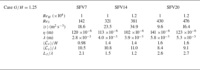

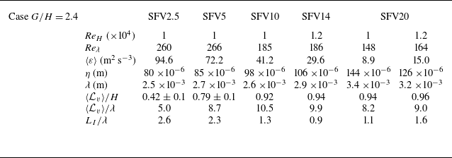

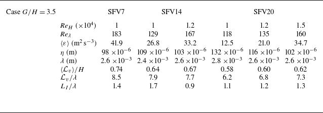


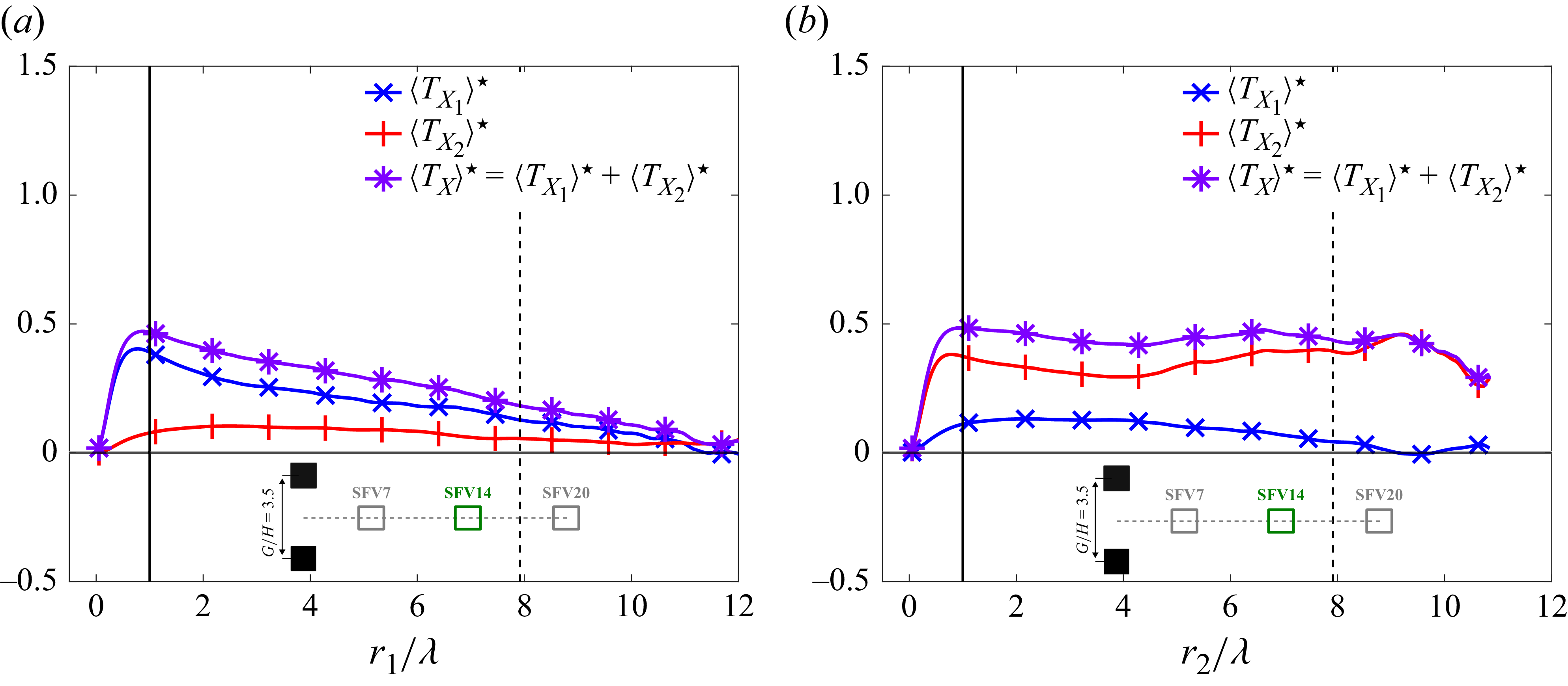


 Open access