


1. Introduction
1.1. Historical perspective
The language of fractal physics has been particularly useful in understanding high Reynolds number flow visualisations that show the simultaneous existence and dynamic evolution of vortical structures ranging from fully three-dimensional large vortices, down to quasi-one-dimensional filaments and even broken structures whose dimensions are less than unity. Many historical references can be found in Yeung & Ravikumar (Reference Yeung and Ravikumar2020), Sreenivasan & Yakhot (Reference Sreenivasan and Yakhot2021) and Jiménez (Reference Jiménez2025); see also Sreenisvasan (Reference Sreenivasan1991), Ishihara et al. (Reference Ishihara, Gotoh and Kaneda2009), Pandit et al. (Reference Pandit, Perlekar and Ray2009), Vassilicos (Reference Vassilicos2015), Yeung et al. (Reference Yeung, Sreenivasan and Pope2018), Dubrulle (Reference Dubrulle2019); Buaria et al. (Reference Buaria, Pumir, Bodenschatz and Yeung2019, Reference Buaria, Pumir, Bodenschatz and Yeung2020), Elsinga et al. (Reference Elsinga, Ishihara and Hunt2020, Reference Elsinga, Ishihara and Hunt2023), Benzi & Toschi (Reference Benzi and Toschi2023), McKeown et al. (Reference McKeown, Pumir, Rubinstein, Brenner and Ostilla-Mónico2023), Mukherjee et al. (Reference Mukherjee, Murugan, Mukherjee and Ray2024), Brewer et al. (Reference Brewer2025) and Kerr (Reference Kerr2025). In their recent report on an extensive series of $32,768^{3}$
computations, Yeung et al. (Reference Yeung, Ravikumar, Uma-Vaideswaran, Dotson, Sreenivasan, Pope, Meneveau and Nichols2025) have pointed out that
$32,768^{3}$
computations, Yeung et al. (Reference Yeung, Ravikumar, Uma-Vaideswaran, Dotson, Sreenivasan, Pope, Meneveau and Nichols2025) have pointed out that
-
Three-dimensional turbulence governed by the Navier–Stokes equations continues to be a grand challenge in computational science, even as leadership-class computing power has recently advanced past exascale.
Theoretical approaches involving fractal geometry and dynamical systems began to intersect in the 1970s and 1980s when conventional descriptions of fluid turbulence as merely quasiperiodic motion (Landau & Lifshitz Reference Landau and Lifshitz1959) began to be questioned: see the history described by Ruelle (Reference Ruelle1995). In their influential paper, Ruelle & Takens (Reference Ruelle and Takens1971) suggested that, as the Reynolds number increased, fluid motion would pass through a generic sequence of bifurcations, which included both periodic and quasi-periodic motion, but whose end state was chaotic motion on a strange attractor. This end state was interpreted as ‘turbulence’, although it is now recognised that this specific sequence is only applicable to tightly confined low-dimensional dynamical systems: see the review by Eckmann (Reference Eckmann1981) and the paper by Libchaber & Maurer (Reference Libchaber and Maurer1982). The applicability of these ideas to the Navier–Stokes equations (NSEs) lay open to question because the theory expounded by Ruelle (Reference Ruelle and Takens1978a
,Reference Ruelle
b
) was valid for finite-dimensional dissipative dynamical systems. The subsequent proof by Foias & Temam (Reference Foias and Temam1979) that the two-dimensional (2-D) NSEs possess a finite-dimensional global attractor $\mathcal{A}$
made the connection secure in this case. Indeed, the further work by Ruelle (Reference Ruelle1982), Constantin & Foias (Reference Constantin and Foias1985) and Constantin (Reference Constantin1987) on Lyapunov exponents of
$\mathcal{A}$
made the connection secure in this case. Indeed, the further work by Ruelle (Reference Ruelle1982), Constantin & Foias (Reference Constantin and Foias1985) and Constantin (Reference Constantin1987) on Lyapunov exponents of $\mathcal{A}$
laid the basis for the sharp (to within logarithms) estimate of the Lyapunov dimension of the 2-D Navier–Stokes global attractor (Constantin, Foias & Temam Reference Constantin, Foias and Temam1988). It must be stressed, however, that this process cannot be followed through for the 3-D NSEs. The Millenium problem of the global regularity of solutions in three dimensions remains open and therefore the existence of a finite-dimensional global attractor remains open. What is known rigorously is the existence of Leray–Hopf weak solutions (Leray Reference Leray1934; Hopf Reference Hopf1951), and it is the correspondence between these and the multifractal model which is the topic of this paper.
$\mathcal{A}$
laid the basis for the sharp (to within logarithms) estimate of the Lyapunov dimension of the 2-D Navier–Stokes global attractor (Constantin, Foias & Temam Reference Constantin, Foias and Temam1988). It must be stressed, however, that this process cannot be followed through for the 3-D NSEs. The Millenium problem of the global regularity of solutions in three dimensions remains open and therefore the existence of a finite-dimensional global attractor remains open. What is known rigorously is the existence of Leray–Hopf weak solutions (Leray Reference Leray1934; Hopf Reference Hopf1951), and it is the correspondence between these and the multifractal model which is the topic of this paper.
The wide range of scales observed in turbulent flows has traditionally been interpreted in terms of a Richardson cascade which involves the transfer of energy from large to smaller scales of motion: see Monin & Yaglom (Reference Monin and Yaglom1975) and also the review by Jiménez (Reference Jiménez2000) who have discussed the effect of intermittency on cascades. Mandelbrot (Reference Meneveau and Sreenivasan1977) popularised the idea that this wide range of scales indicates an underlying fractal geometric structure, but it also became increasingly clear that the idea of a monofractal system with just a single dimension was not enough to provide an adequate description. Parisi & Frisch (Reference Parisi and Frisch1985) then interpreted these cascade processes in multifractal terms where there is a continuous spectrum of dimensions. A parameter designated as $h$
, which appears naturally in the invariant scaling of the underlying Euler equations (see (1.3)), was used as a local scaling exponent, with each value of
$h$
, which appears naturally in the invariant scaling of the underlying Euler equations (see (1.3)), was used as a local scaling exponent, with each value of $h$
belonging to a given fractal set of dimension
$h$
belonging to a given fractal set of dimension $D(h)$
. This has become known as the multi-fractal model (MFM) of turbulence: expositions can be found in Meneveau & Sreenivasan (Reference Meneveau and Sreenivasan1991), Frisch (Reference Frisch1995), Bohr et al. (Reference Bohr, Jensen, Paladin and Vulpiani1998), Boffetta et al. (Reference Boffetta, Mazzino and Vulpiani2008), Benzi & Biferale (Reference Benzi, Biferale and Toschi2009) and Frisch (Reference Frisch2016), together with two series of lecture notes by Eyink (Reference Eyink and Peng2008) and Benzi & Toschi (Reference Benzi and Toschi2023). In fact, multifractal scaling has a broad application in the physical sciences (Stanley & Meakin Reference Stanley and Meakin1988). While hydrodynamic turbulence is perhaps its most prominent example, other turbulent systems must be included, such as passive scalar fields (Prasad et al. Reference Prasad, Meneveau and Sreenivasan1988) and bacterial suspensions (Liu & Lin Reference Meneveau and Sreenivasan2012).
$D(h)$
. This has become known as the multi-fractal model (MFM) of turbulence: expositions can be found in Meneveau & Sreenivasan (Reference Meneveau and Sreenivasan1991), Frisch (Reference Frisch1995), Bohr et al. (Reference Bohr, Jensen, Paladin and Vulpiani1998), Boffetta et al. (Reference Boffetta, Mazzino and Vulpiani2008), Benzi & Biferale (Reference Benzi, Biferale and Toschi2009) and Frisch (Reference Frisch2016), together with two series of lecture notes by Eyink (Reference Eyink and Peng2008) and Benzi & Toschi (Reference Benzi and Toschi2023). In fact, multifractal scaling has a broad application in the physical sciences (Stanley & Meakin Reference Stanley and Meakin1988). While hydrodynamic turbulence is perhaps its most prominent example, other turbulent systems must be included, such as passive scalar fields (Prasad et al. Reference Prasad, Meneveau and Sreenivasan1988) and bacterial suspensions (Liu & Lin Reference Meneveau and Sreenivasan2012).
1.2. A reconciliation between the MFM and the NSEs
It has become part of the folklore of turbulence that no mathematical relation exists between the MFM, which is applicable to statistically steady, homogeneous, isotropic turbulence (HIT), and the forced incompressible 3-D NSEs
 \begin{equation} \left (\partial _{t} + {\boldsymbol{u}}\boldsymbol{\cdot }\boldsymbol{\nabla }\right ) {\boldsymbol{u}} + \boldsymbol{\nabla }\!p = \nu \Delta {\boldsymbol{u}} + \boldsymbol{f}({\boldsymbol{x}})\quad \mbox{div}\,{\boldsymbol{u}} = 0, \end{equation}
which are evolution equations requiring specific initial conditions. In (1.1) $\boldsymbol{u}$
,
$\boldsymbol{u}$
, $p$
and
$p$
and $\nu$
are respectively the velocity field, pressure and viscosity of the fluid, while
$\nu$
are respectively the velocity field, pressure and viscosity of the fluid, while $\boldsymbol{f} (\boldsymbol{x})$
is the body forcing. Building on piecemeal attempts in this direction (Dubrulle & Gibbon Reference Dubrulle and Gibbon2022; Gibbon Reference Gibbon2023), this paper will demonstrate that a reconciliation between the two theories is possible. There are two ways of approaching this reconciliation, both of which involve a result of Paladin & Vulpiani (Reference Paladin and Vulpiani1987a
,
Reference Paladin and Vulpianib
) who used the MFM formalism to introduce a length scale into Navier–Stokes turbulence, which we call the PaV scale
$\boldsymbol{f} (\boldsymbol{x})$
is the body forcing. Building on piecemeal attempts in this direction (Dubrulle & Gibbon Reference Dubrulle and Gibbon2022; Gibbon Reference Gibbon2023), this paper will demonstrate that a reconciliation between the two theories is possible. There are two ways of approaching this reconciliation, both of which involve a result of Paladin & Vulpiani (Reference Paladin and Vulpiani1987a
,
Reference Paladin and Vulpianib
) who used the MFM formalism to introduce a length scale into Navier–Stokes turbulence, which we call the PaV scale $\eta _{h,\textit{pa}v}$
(to avoid confusion with potential vorticity). In terms of the Reynolds number
$\eta _{h,\textit{pa}v}$
(to avoid confusion with potential vorticity). In terms of the Reynolds number $\textit{Re}$
the inverse PaV scale is
$\textit{Re}$
the inverse PaV scale is
 \begin{equation} \ell \eta _{h,\textit{pa}v}^{-1} = \mathit{Re}^{{1}/({1+h})}, \end{equation}
where the definition of the Reynolds number in Paladin & Vulpiani (Reference Paladin and Vulpiani1987a
,
Reference Paladin and Vulpianib
) was originally based on the energy dissipation rate and was derived using phenomenological arguments rather than directly from the NSEs. Moreover, the velocity field was assumed to be statistically stationary. To establish a mathematical relation between the MFM and the NSEs, it is critical that we use a definition of the PaV scale that is not only based on the NSEs but which is also expressed in terms of a NS-based Reynolds number. Let us consider the invariant scaling of the Euler equations. Let $\eta$
be an inner length scale
$\eta$
be an inner length scale $0 \lt \eta \leqslant \ell$
and
$0 \lt \eta \leqslant \ell$
and $\ell$
an outer scale which, in the periodic case, would be the box size
$\ell$
an outer scale which, in the periodic case, would be the box size $\ell = L$
. Consider the incompressible Euler equations in dimensional variables
$\ell = L$
. Consider the incompressible Euler equations in dimensional variables ${\boldsymbol{u}}({\boldsymbol{x}},\,t)$
. If we introduce a typical velocity
${\boldsymbol{u}}({\boldsymbol{x}},\,t)$
. If we introduce a typical velocity $U_{0}$
, a frequency
$U_{0}$
, a frequency $\varpi _{0} = U_{0}\ell ^{-1}$
and the dimensionless parameter
$\varpi _{0} = U_{0}\ell ^{-1}$
and the dimensionless parameter $\lambda = \ell \eta ^{-1} \geqslant 1$
, then the dimensionless set of primed variables
$\lambda = \ell \eta ^{-1} \geqslant 1$
, then the dimensionless set of primed variables ${\boldsymbol{u}}'({\boldsymbol{x}}',\,t')$
defined by (
${\boldsymbol{u}}'({\boldsymbol{x}}',\,t')$
defined by ( $h+1 \gt 0$
)
$h+1 \gt 0$
)
 \begin{equation} {\boldsymbol{x}}' = \lambda \ell ^{-1}{\boldsymbol{x}},\quad t' = \lambda ^{1-h}\varpi _{0}t, \quad {\boldsymbol{u}} = U_{0}\lambda ^{-h}{\boldsymbol{u}}', \end{equation}
transforms the Euler equations in dimensional variables into the dimensionless Euler equations in primed variables. While the Euler equations are invariant under the transformation in (1.3) for every value of $\lambda \geqslant 1$
, the NSEs are not. Instead, direct application of (1.3) to the NSEs (1.1) shows that
$\lambda \geqslant 1$
, the NSEs are not. Instead, direct application of (1.3) to the NSEs (1.1) shows that $\eta =\eta _{h,\textit{pa}v}$
is that particular value of
$\eta =\eta _{h,\textit{pa}v}$
is that particular value of $\eta$
for which the NSEs in dimensional variables
$\eta$
for which the NSEs in dimensional variables ${\boldsymbol{u}}({\boldsymbol{x}},\,t)$
and with corresponding Reynolds number
${\boldsymbol{u}}({\boldsymbol{x}},\,t)$
and with corresponding Reynolds number $\textit{Re}=\ell U_{0}\nu ^{-1}$
, are transformed into the NSEs in dimensionless variables
$\textit{Re}=\ell U_{0}\nu ^{-1}$
, are transformed into the NSEs in dimensionless variables ${\boldsymbol{u}}'({\boldsymbol{x}}',\,t')$
with Reynolds number equal to unity
${\boldsymbol{u}}'({\boldsymbol{x}}',\,t')$
with Reynolds number equal to unity
 \begin{equation} \left (\partial _{t'} + {\boldsymbol{u}}'\boldsymbol{\cdot }\boldsymbol{\nabla }'\right ) {\boldsymbol{u}}' + \boldsymbol{\nabla }'\!p' = \Delta '{\boldsymbol{u}}' + \boldsymbol{f}'({\boldsymbol{x}}')\quad \mbox{div}'{\boldsymbol{u}}' = 0. \end{equation}
Thus, $\eta =\eta _{h,\textit{pa}v}$
occurs exactly where the inertial and dissipative terms balance. This interpretation of
$\eta =\eta _{h,\textit{pa}v}$
occurs exactly where the inertial and dissipative terms balance. This interpretation of $\eta _{h,\textit{pa}v}$
has been used, in particular, to obtain ‘fusion rules’ for the statistical correlations between the inertial-range increments and the derivatives of the velocity (Benzi et al. Reference Benzi, Biferale and Toschi1998; Friedrich et al. Reference Friedrich, Margazoglou, Biferale and Grauer2018). Depending on the allowed range of
$\eta _{h,\textit{pa}v}$
has been used, in particular, to obtain ‘fusion rules’ for the statistical correlations between the inertial-range increments and the derivatives of the velocity (Benzi et al. Reference Benzi, Biferale and Toschi1998; Friedrich et al. Reference Friedrich, Margazoglou, Biferale and Grauer2018). Depending on the allowed range of $h$
we see that the invariant scaling transformation of the Euler equations lies behind the onset of NS-turbulence as a multi-scale phenomenon. Kolmogorov’s theory (Frisch Reference Frisch1995), known as K41, restricts this to a single scale by insisting on
$h$
we see that the invariant scaling transformation of the Euler equations lies behind the onset of NS-turbulence as a multi-scale phenomenon. Kolmogorov’s theory (Frisch Reference Frisch1995), known as K41, restricts this to a single scale by insisting on $h = {{1}/{3}}$
but, as we see below, the MFM allows a wider spread of
$h = {{1}/{3}}$
but, as we see below, the MFM allows a wider spread of $h$
. Moreover, we shall also see that the PaV scale is much more than just a bridge between the Euler and the NSEs because it also stitches together the MFM and Leray’s weak solution formalism of the NSEs (Leray Reference Leray1934; Robinson et al. Reference Robinson, Rodrigo and Sadowski2016) which is manifest as sequences of bounded time averages (Gibbon Reference Gibbon2019, Reference Gibbon2020).
$h$
. Moreover, we shall also see that the PaV scale is much more than just a bridge between the Euler and the NSEs because it also stitches together the MFM and Leray’s weak solution formalism of the NSEs (Leray Reference Leray1934; Robinson et al. Reference Robinson, Rodrigo and Sadowski2016) which is manifest as sequences of bounded time averages (Gibbon Reference Gibbon2019, Reference Gibbon2020).
Our first approach, expounded in § 4.1, is to adapt the method of Dubrulle & Gibbon (Reference Dubrulle and Gibbon2022) for evaluating the higher norms of the velocity gradient by using the Euler scaling invariance in the probabilistic sense of the MFM at the wavenumber $k_{h,\textit{pa}v} = \eta _{h,\textit{pa}v}^{-1}$
. Selecting only this wavenumber in the spectrum with a variation in
$k_{h,\textit{pa}v} = \eta _{h,\textit{pa}v}^{-1}$
. Selecting only this wavenumber in the spectrum with a variation in $h$
, and then averaging over
$h$
, and then averaging over $h$
, circumvents the difficulty with the Kolmogorov picture where the spectrum is divided into the inertial range and the dissipation range, a division which conventional Sobolev methods of NS-analysis do not recognise. Comparison with time-averaged results from the NSEs in § 4.2 shows that the results are consistent with the four-fifths law; namely that the multifractal spectrum (co-dimension) obeys the inequality
$h$
, circumvents the difficulty with the Kolmogorov picture where the spectrum is divided into the inertial range and the dissipation range, a division which conventional Sobolev methods of NS-analysis do not recognise. Comparison with time-averaged results from the NSEs in § 4.2 shows that the results are consistent with the four-fifths law; namely that the multifractal spectrum (co-dimension) obeys the inequality $C(h) \geqslant 1-3h$
, with
$C(h) \geqslant 1-3h$
, with $h$
lying in the range
$h$
lying in the range $-{{2}/{3}} \leqslant h \leqslant {{1}/{3}}$
. This corresponds to the dissipation range. The typical velocity field
$-{{2}/{3}} \leqslant h \leqslant {{1}/{3}}$
. This corresponds to the dissipation range. The typical velocity field $U_{0}$
in (1.3) is chosen as the root-mean-square velocity field of the NSEs, as in (3.2), and the outer scale
$U_{0}$
in (1.3) is chosen as the root-mean-square velocity field of the NSEs, as in (3.2), and the outer scale $\ell$
is chosen as the box scale
$\ell$
is chosen as the box scale $L$
of the NSEs. The outer scale
$L$
of the NSEs. The outer scale $\ell$
could equivalently be taken as the integral scale of the velocity or the characteristic length scale of the forcing. Such choices would yield an additional prefactor
$\ell$
could equivalently be taken as the integral scale of the velocity or the characteristic length scale of the forcing. Such choices would yield an additional prefactor $(L/\ell )^3$
in the Navier–Stokes estimates provided in § 3, but would not change the way the estimates scale with
$(L/\ell )^3$
in the Navier–Stokes estimates provided in § 3, but would not change the way the estimates scale with $\textit{Re}$
, which is the key element in our analysis.
$\textit{Re}$
, which is the key element in our analysis.
The second idea also involves the PaV scale but in the reverse order. In § 4.2 the parameter $m$
in the
$m$
in the $L^{2m}$
-norms of the velocity gradient is treated as if it were the sliding focus control of a telescope through which one can zoom in and out on intermittent events. This allows us to mimic weak solution time averages as if they exist on a multifractal set
$L^{2m}$
-norms of the velocity gradient is treated as if it were the sliding focus control of a telescope through which one can zoom in and out on intermittent events. This allows us to mimic weak solution time averages as if they exist on a multifractal set $\mathbb{F}_{m}$
whose range of dimensions is
$\mathbb{F}_{m}$
whose range of dimensions is ${\mathfrak{D}_{m}}=3/m$
. Under the assumption that the NS flow has settled into a fully developed state,
${\mathfrak{D}_{m}}=3/m$
. Under the assumption that the NS flow has settled into a fully developed state, $\mathfrak{D}_{m}$
can then be compared with
$\mathfrak{D}_{m}$
can then be compared with $D(h)$
. This gives a simple relation between the scaling exponent
$D(h)$
. This gives a simple relation between the scaling exponent $h$
and
$h$
and $m$
. The range
$m$
. The range $1 \leqslant m \leqslant \infty$
corresponds to
$1 \leqslant m \leqslant \infty$
corresponds to $-{{2}/{3}} \leqslant h_{\textit{min}} \leqslant {{1}/{3}}$
, which gives a cutoff deep in the dissipation range. The PaV scale
$-{{2}/{3}} \leqslant h_{\textit{min}} \leqslant {{1}/{3}}$
, which gives a cutoff deep in the dissipation range. The PaV scale $\eta _{h,\textit{pa}v}$
then re-emerges as the best estimate over all
$\eta _{h,\textit{pa}v}$
then re-emerges as the best estimate over all $m$
for the natural length scale of the problem.
$m$
for the natural length scale of the problem.
1.3. Connection with two open questions
The invariance of the Euler equations and their correspondence with the NSEs also touches recent work on Onsager’s conjecture (Onsager Reference Onsager1949; Eyink Reference Eyink and Peng1995, Reference Eyink and Peng2024; Eyink & Peng Reference Eyink and Peng2025). De Lellis & Székelyhidi (Reference De Lellis and Székelyhidi2009, Reference De Lellis and Székelyhidi2010) have shown that the incompressible 3-D Euler equations possess `wild solutions’ whose kinetic energy $e(t)$
does not have to be decreasing in time and may have compact support, thus suggesting a strong degree of irregularity. These solutions, found by the method of convex integration, imply that the fluid could suddenly burst into rapid motion, and then return to rest after a finite period of time. An equivalent result has been proved for the NSEs by Buckmaster & Vicol (Reference Buckmaster and Vicol2019, Reference Buckmaster and Vicol2021). These solutions belong to the space
$e(t)$
does not have to be decreasing in time and may have compact support, thus suggesting a strong degree of irregularity. These solutions, found by the method of convex integration, imply that the fluid could suddenly burst into rapid motion, and then return to rest after a finite period of time. An equivalent result has been proved for the NSEs by Buckmaster & Vicol (Reference Buckmaster and Vicol2019, Reference Buckmaster and Vicol2021). These solutions belong to the space $W^{1,1}$
for all time, which means that both
$W^{1,1}$
for all time, which means that both $\|{\boldsymbol{u}}\|_{1}$
and
$\|{\boldsymbol{u}}\|_{1}$
and $\|\boldsymbol{\nabla }{\boldsymbol{u}}\|_{1}$
remain finite. However,
$\|\boldsymbol{\nabla }{\boldsymbol{u}}\|_{1}$
remain finite. However, $\|\boldsymbol{\nabla }{\boldsymbol{u}}\|_{2}$
is not integrable in time so they do not satisfy a Leray–Hopf-type energy inequality. The suggestion that wild solutions may be the root cause of NS turbulence is both speculative and controversial but it is nevertheless an interesting and important open question. The magazine article by Eyink et al. (Reference Eyink and Peng2025) covers a wide range of opinion by several authors over the issue of whether the Buckmaster–Vicol result is physically relevant to hydrodynamics. What is clear is that this issue has yet to be settled. A further argument is that the flaw lies in the NSEs themselves. The suggestion that thermal noise could make the deterministic version of the incompressible NSEs inadequate to describe the dissipation range of turbulence was first raised by Ruelle (Reference Ruelle1979, Reference Ruelle1995). This is precisely the region covered by the PaV scale. More recently, Bandak et al. (Reference Bandak, Goldenfeld, Mailybaev and Eyink2022, Reference Bandak, Mailybaev, Eyink and Goldenfeld2024) have gone further by arguing that in molecular fluids Eulerian spontaneous stochasticity (Gawȩdzki Reference Gawȩdzki2008; Thalabard et al. Reference Thalabard, Bec and Mailybaev2020) is triggered by thermal noise in 3-D Navier–Stokes turbulence at high Reynolds numbers and that this directly alters the turbulent dissipation range below the Kolmogorov scale. Bandak et al. (Reference Bandak, Mailybaev, Eyink and Goldenfeld2024) conclude that the NSEs should be replaced by a Landau–Lifshitz-type set of equations which is comprised of the incompressible NSEs plus an additive fluctuating stress term proportional to
$\|\boldsymbol{\nabla }{\boldsymbol{u}}\|_{2}$
is not integrable in time so they do not satisfy a Leray–Hopf-type energy inequality. The suggestion that wild solutions may be the root cause of NS turbulence is both speculative and controversial but it is nevertheless an interesting and important open question. The magazine article by Eyink et al. (Reference Eyink and Peng2025) covers a wide range of opinion by several authors over the issue of whether the Buckmaster–Vicol result is physically relevant to hydrodynamics. What is clear is that this issue has yet to be settled. A further argument is that the flaw lies in the NSEs themselves. The suggestion that thermal noise could make the deterministic version of the incompressible NSEs inadequate to describe the dissipation range of turbulence was first raised by Ruelle (Reference Ruelle1979, Reference Ruelle1995). This is precisely the region covered by the PaV scale. More recently, Bandak et al. (Reference Bandak, Goldenfeld, Mailybaev and Eyink2022, Reference Bandak, Mailybaev, Eyink and Goldenfeld2024) have gone further by arguing that in molecular fluids Eulerian spontaneous stochasticity (Gawȩdzki Reference Gawȩdzki2008; Thalabard et al. Reference Thalabard, Bec and Mailybaev2020) is triggered by thermal noise in 3-D Navier–Stokes turbulence at high Reynolds numbers and that this directly alters the turbulent dissipation range below the Kolmogorov scale. Bandak et al. (Reference Bandak, Mailybaev, Eyink and Goldenfeld2024) conclude that the NSEs should be replaced by a Landau–Lifshitz-type set of equations which is comprised of the incompressible NSEs plus an additive fluctuating stress term proportional to $\mbox{div}\,\boldsymbol{\xi }$
, where
$\mbox{div}\,\boldsymbol{\xi }$
, where $\boldsymbol{\xi }$
is modelled as a mean-zero Gaussian random field with a given ensemble average. The range of scales over which it is conjectured that these thermal effects take place not only includes the dissipation range but also reaches into the inertial range, which illustrates why it is important that this issue is resolved. Moreover, if this argument turns out to be correct then it will change the direction of analysis in fluid dynamics. The search for a regularity proof of the 3-D deterministic NSEs, although unsuccessful, has been one of the major issues in rigorous fluid dynamics in the past generation (Leray Reference Leray1934; Foias, Guillopé & Temam Reference Friedrich, Margazoglou, Biferale and Grauer1981; Robinson et al. Reference Robinson, Rodrigo and Sadowski2016; Gibbon Reference Gibbon2019). In contrast, the Landau–Lifschitz equations, having been designed as mesoscopic field equations with a high-wavenumber cutoff, have been proved to have strong, pathwise-unique solutions (Flandoli Reference Flandoli2008; Eyink Reference Eyink and Peng2024).
$\boldsymbol{\xi }$
is modelled as a mean-zero Gaussian random field with a given ensemble average. The range of scales over which it is conjectured that these thermal effects take place not only includes the dissipation range but also reaches into the inertial range, which illustrates why it is important that this issue is resolved. Moreover, if this argument turns out to be correct then it will change the direction of analysis in fluid dynamics. The search for a regularity proof of the 3-D deterministic NSEs, although unsuccessful, has been one of the major issues in rigorous fluid dynamics in the past generation (Leray Reference Leray1934; Foias, Guillopé & Temam Reference Friedrich, Margazoglou, Biferale and Grauer1981; Robinson et al. Reference Robinson, Rodrigo and Sadowski2016; Gibbon Reference Gibbon2019). In contrast, the Landau–Lifschitz equations, having been designed as mesoscopic field equations with a high-wavenumber cutoff, have been proved to have strong, pathwise-unique solutions (Flandoli Reference Flandoli2008; Eyink Reference Eyink and Peng2024).
2. The multifractal model of turbulence
The MFM is well established in the literature, so we provide only the briefest of summaries (Frisch Reference Frisch1995; Bohr et al. Reference Bohr, Jensen, Paladin and Vulpiani1998; Boffetta et al. Reference Boffetta, Mazzino and Vulpiani2008; Eyink Reference Eyink and Peng2008; Benzi & Biferale Reference Benzi, Biferale and Toschi2009; Benzi & Toschi Reference Benzi and Toschi2023). The $p$
th-order longitudinal velocity structure function
$p$
th-order longitudinal velocity structure function $S_{p}$
at a point
$S_{p}$
at a point $\boldsymbol{x}$
in an HIT flow is defined as
$\boldsymbol{x}$
in an HIT flow is defined as
 \begin{equation} S_{p}(r) = \left \langle \left \{\left [{\boldsymbol{u}}({\boldsymbol{x}}+\boldsymbol{r}) - {\boldsymbol{u}}({\boldsymbol{x}})\right ]\boldsymbol{\cdot }\hat {\boldsymbol{r}}\right \}^{p}\right \rangle _{\textit{stat}.av.}, \end{equation}
where $r$
is the radius of the sphere centred at
$r$
is the radius of the sphere centred at $\boldsymbol{x}$
. While the details of the statistical average are of little concern, the scaling properties of
$\boldsymbol{x}$
. While the details of the statistical average are of little concern, the scaling properties of $S_{p}$
in the infinite Reynolds number limit are crucial as they revolve around the invariance property of the incompressible Euler equations. The K41 formalism assumes that
$S_{p}$
in the infinite Reynolds number limit are crucial as they revolve around the invariance property of the incompressible Euler equations. The K41 formalism assumes that $S_{p}$
depends only on
$S_{p}$
depends only on $r$
and the energy dissipation rate
$r$
and the energy dissipation rate $\varepsilon = \nu L^{-3}\int _{V}|\boldsymbol{\nabla }{\boldsymbol{u}}|^{2}\,\text{d}V$
. Since the product
$\varepsilon = \nu L^{-3}\int _{V}|\boldsymbol{\nabla }{\boldsymbol{u}}|^{2}\,\text{d}V$
. Since the product $\varepsilon r$
has the same units as
$\varepsilon r$
has the same units as $u^3$
, the only scaling consistent with physical units is
$u^3$
, the only scaling consistent with physical units is $S_{p} \sim (\varepsilon r)^{p/3}$
. According to Frisch (Reference Frisch1995), the symbol
$S_{p} \sim (\varepsilon r)^{p/3}$
. According to Frisch (Reference Frisch1995), the symbol $\sim$
means ‘scales like’. This agrees with the exact result
$\sim$
means ‘scales like’. This agrees with the exact result $S_{3} = - {4}\varepsilon r/{5}$
, which is known as the four-fifths law. While the result is elegant and satisfying, experimental and numerical data indicate that
$S_{3} = - {4}\varepsilon r/{5}$
, which is known as the four-fifths law. While the result is elegant and satisfying, experimental and numerical data indicate that $S_{\!p}$
scales like
$S_{\!p}$
scales like $S_{\!p}\sim r^{\zeta _{\!p}}$
, where the exponents
$S_{\!p}\sim r^{\zeta _{\!p}}$
, where the exponents $\zeta _{\!p}$
deviate from linear in
$\zeta _{\!p}$
deviate from linear in $p$
by lying on a concave curve that, for
$p$
by lying on a concave curve that, for $p\geqslant 3$
, stays below the line
$p\geqslant 3$
, stays below the line $p/{3}$
, a deviation which is attributed to intermittency (Frisch Reference Frisch1995). To explain this, Parisi & Frisch (Reference Parisi and Frisch1985) adapted the K41 formalism by relaxing the requirement that, for small
$p/{3}$
, a deviation which is attributed to intermittency (Frisch Reference Frisch1995). To explain this, Parisi & Frisch (Reference Parisi and Frisch1985) adapted the K41 formalism by relaxing the requirement that, for small $r$
, the velocity increment
$r$
, the velocity increment $\vert {\boldsymbol{u}}({\boldsymbol{x}}+\boldsymbol{r})-{\boldsymbol{u}}({\boldsymbol{x}})\vert$
scales as
$\vert {\boldsymbol{u}}({\boldsymbol{x}}+\boldsymbol{r})-{\boldsymbol{u}}({\boldsymbol{x}})\vert$
scales as $r^h$
with
$r^h$
with $h={{1}/{3}}$
. Instead, they allowed the scaling exponent
$h={{1}/{3}}$
. Instead, they allowed the scaling exponent $h$
to fluctuate. They achieved this by writing down the probability of observing a given value of
$h$
to fluctuate. They achieved this by writing down the probability of observing a given value of $h$
at the scale
$h$
at the scale $r$
in the form
$r$
in the form
 \begin{equation} P_{r}(h) \sim r^{C(h)}, \end{equation}
where each value of $h$
belongs to a given fractal set of dimension
$h$
belongs to a given fractal set of dimension $D(h)$
. The co-dimension
$D(h)$
. The co-dimension $C(h)= 3 - D(h)$
plays the role of the multifractal spectrum in the large deviation theory version expounded by Eyink (Reference Eyink and Peng2008). Interpreting (2.1) as an average over the probability
$C(h)= 3 - D(h)$
plays the role of the multifractal spectrum in the large deviation theory version expounded by Eyink (Reference Eyink and Peng2008). Interpreting (2.1) as an average over the probability $P_r(h)$
, and by applying a steepest descent argument, one finds the following relation for the exponent
$P_r(h)$
, and by applying a steepest descent argument, one finds the following relation for the exponent $\zeta _{\!p}$
:
$\zeta _{\!p}$
:
 \begin{equation} \zeta _{p} = \lim _{r\to 0}\left (\frac {\ln S_{p}}{\ln (\varepsilon r)}\right )\!, \quad \mbox{where}\quad \zeta _{p} = \inf _{h}\left [hp + C(h)\right ]\!. \end{equation}
Thus, $\zeta _{\!p}$
and
$\zeta _{\!p}$
and $C(h)$
are connected through a Legendre transform. Note that, when
$C(h)$
are connected through a Legendre transform. Note that, when $D(h)=3$
, we recover the standard K41 result that
$D(h)=3$
, we recover the standard K41 result that $S_{p} \sim (\varepsilon r)^{hp}$
. The four-fifths law requires
$S_{p} \sim (\varepsilon r)^{hp}$
. The four-fifths law requires $\zeta _{3} = 1$
, thus leading to inequalities for
$\zeta _{3} = 1$
, thus leading to inequalities for $D(h)$
and
$D(h)$
and $C(h)$
 \begin{equation} C(h) \geqslant 1 - 3h \quad \Rightarrow \quad D(h) \leqslant 3h + 2. \end{equation}
An alternative definition of multifractality is based on the fluctuations of energy dissipation (Meneveau & Sreenivasan Reference Meneveau and Sreenivasan1991; Aurell et al. Reference Aurell, Frisch, Lutsko and Vergassola1992; Frisch Reference Frisch1995). It assumes the existence of a continuous range of scaling exponents $a$
such that the local average of the energy dissipation rate over a ball of radius
$a$
such that the local average of the energy dissipation rate over a ball of radius $r$
scales like
$r$
scales like $r^a$
over a fractal set of dimension
$r^a$
over a fractal set of dimension $\mathcal{F}(a)$
. Kolmogorov’s refined similarity hypothesis allows a connection to be established between the two definitions of multifractality; in particular,
$\mathcal{F}(a)$
. Kolmogorov’s refined similarity hypothesis allows a connection to be established between the two definitions of multifractality; in particular, $h=a/3$
and
$h=a/3$
and $D(h)=\mathcal{F}(a)$
(Aurell et al. Reference Aurell, Frisch, Lutsko and Vergassola1992; Frisch Reference Frisch1995). Finally, it is important to note that the MFM describes the scaling properties of the velocity field and the local energy dissipation but does not provide any information on the geometric structure of the flow. To see how the multifractal formalism fits with the NSEs requires an examination of the
$D(h)=\mathcal{F}(a)$
(Aurell et al. Reference Aurell, Frisch, Lutsko and Vergassola1992; Frisch Reference Frisch1995). Finally, it is important to note that the MFM describes the scaling properties of the velocity field and the local energy dissipation but does not provide any information on the geometric structure of the flow. To see how the multifractal formalism fits with the NSEs requires an examination of the $L^{2m}$
-norms of the velocity gradient, which we do in the next section.
$L^{2m}$
-norms of the velocity gradient, which we do in the next section.
3. $L^{2m}$
-norms of the Navier–Stokes velocity gradient
$L^{2m}$
-norms of the Navier–Stokes velocity gradient

The behaviour of the pointwise in time energy dissipation rate $\varepsilon = \nu L^{-3}{\int _{V}}|\boldsymbol{\nabla }{\boldsymbol{u}}|^{2}\,\text{d}V$
has been one of the primary goals in turbulence research (Verma Reference Verma2019). Based on the ideas of Leray (Reference Leray1934) and Hopf (Reference Hopf1951), the energy inequality in a 3-D periodic domain is
$\varepsilon = \nu L^{-3}{\int _{V}}|\boldsymbol{\nabla }{\boldsymbol{u}}|^{2}\,\text{d}V$
has been one of the primary goals in turbulence research (Verma Reference Verma2019). Based on the ideas of Leray (Reference Leray1934) and Hopf (Reference Hopf1951), the energy inequality in a 3-D periodic domain is
 \begin{align} \frac 1{2} {\int _{V}} \left (|{\boldsymbol{u}}({\boldsymbol{x}},\,t)|^{2} - |{\boldsymbol{u}}({\boldsymbol{x}},\,0)|^{2}\right ) \,\text{d}V + \nu \int _{0}^{t}{\int _{V}}|\boldsymbol{\nabla }{\boldsymbol{u}}({\boldsymbol{x}},\,\tau )|^{2}\,\text{d}V\,\text{d}\tau \leqslant \int _{0}^{t}{\int _{V}} {\boldsymbol{u}}\boldsymbol{\cdot }\boldsymbol{f}\,\text{d}V\,\text{d}\tau . \end{align}
Note that this is an inequality, not an equality, and is valid for weak solutions of the 3-D NSEs: see also Caffarelli, Kohn & Nirenberg (Reference Caffarelli, Kohn and Nirenberg1982) for a wider definition. Behind it lies a sophisticated theory of weak convergence properties that can be found in standard textbooks such as Robinson et al. (Reference Robinson, Rodrigo and Sadowski2016). Doering & Foias (Reference Doering and Foias2002) showed how to translate estimates based on the forcing $\boldsymbol{f}$
(whose
$\boldsymbol{f}$
(whose $L^{2}$
-norm feeds into the Grashof number
$L^{2}$
-norm feeds into the Grashof number $Gr$
) into estimates based on the Reynolds number
$Gr$
) into estimates based on the Reynolds number $\textit{Re} = U_{0}L/\nu$
, which is itself based on a space–time-averaged velocity field
$\textit{Re} = U_{0}L/\nu$
, which is itself based on a space–time-averaged velocity field $U_{0}$
, and the time-average
$U_{0}$
, and the time-average $\left \langle \boldsymbol{\cdot }\right \rangle _{T}$
 \begin{equation} U_{0}^{2} = L^{-3}\big \langle \|{\boldsymbol{u}}\|_{2}^{2}\big \rangle _{T},\quad \mbox{with}\quad \left \langle \boldsymbol{\cdot }\right \rangle _{T}=\frac {1}{T}\int _{0}^{T}\boldsymbol{\cdot }\,\text{d}t. \end{equation}
The Reynolds number $\textit{Re} = U_{0}L/\nu$
has a solid basis because
$\textit{Re} = U_{0}L/\nu$
has a solid basis because $U_{0}$
is bounded for all time. The time-averaged energy dissipation rate for all smooth Navier–Stokes initial conditions and square integrable forcing is (Doering & Foias Reference Doering and Foias2002)
$U_{0}$
is bounded for all time. The time-averaged energy dissipation rate for all smooth Navier–Stokes initial conditions and square integrable forcing is (Doering & Foias Reference Doering and Foias2002)
 \begin{equation} \left \langle \varepsilon \right \rangle _{T} = \nu L^{-3}\left \langle {\int _{V}} |\boldsymbol{\nabla }{\boldsymbol{u}}|^{2}\,\text{d}V\right \rangle _{T} \leqslant L^{-4}\nu ^{3}\textit{Re}^{3}. \end{equation}
Inequality (3.3) leads to the standard inverse Kolmogorov length estimate $L\lambda _{k}^{-1} \leqslant \textit{Re}^{3/4}$
, consistent with K41. However, it does not take account of strong intermittent events that are washed over by the spatial
$L\lambda _{k}^{-1} \leqslant \textit{Re}^{3/4}$
, consistent with K41. However, it does not take account of strong intermittent events that are washed over by the spatial $L^2$
average in (3.3). To address this issue we require higher
$L^2$
average in (3.3). To address this issue we require higher $L^{2m}$
-norms of the velocity gradient tensor
$L^{2m}$
-norms of the velocity gradient tensor
 \begin{equation} \|\boldsymbol{\nabla }{\boldsymbol{u}}\|_{2m}\equiv \left ({\int _{V}} |\boldsymbol{\nabla }{\boldsymbol{u}}|^{2m}\,\text{d}V\right )^{1/2m},\quad 1 \leqslant m \leqslant \infty . \end{equation}
From the evolution of a trefoil vortex knot for $\nu = 3.12\times 10^{-5}$
, evidence appears of intermittent events at
$\nu = 3.12\times 10^{-5}$
, evidence appears of intermittent events at $t\approx 110$
for
$t\approx 110$
for $m\geqslant 5$
; courtesy of R. M. Kerr (Reference Kerr2025). The vertical axis is
$m\geqslant 5$
; courtesy of R. M. Kerr (Reference Kerr2025). The vertical axis is $F_{m}^{\alpha _{m}}$
defined in (3.7) for
$F_{m}^{\alpha _{m}}$
defined in (3.7) for $d=3$
which represent scaled
$d=3$
which represent scaled $L^{2m}$
-norms of the velocity gradient.
$L^{2m}$
-norms of the velocity gradient.

For values of $m$
near unity the integral is insensitive to strong intermittent events: the near
$m$
near unity the integral is insensitive to strong intermittent events: the near $L^2$
spatial average washes over the most intense regions of
$L^2$
spatial average washes over the most intense regions of $\boldsymbol{\nabla }{\boldsymbol{u}}$
with relatively little effect – see figure 1. However, as the value of
$\boldsymbol{\nabla }{\boldsymbol{u}}$
with relatively little effect – see figure 1. However, as the value of $m$
is raised, regions of greater intensity begin to dominate, and eventually at
$m$
is raised, regions of greater intensity begin to dominate, and eventually at $m=\infty$
the most intense point of all completely dominates the integral
$m=\infty$
the most intense point of all completely dominates the integral
 \begin{equation} \begin{array}{ll} m=1\, & {\textrm {corresponds to a root-mean-square average,}}\\ m\,{\textrm {finite but large}}\, & {\textrm {corresponds to the more intense structures,}}\\ m=\infty \, & {\textrm {corresponds to the most intense point.}} \end{array} \end{equation}
Thus, the sliding scale of $m = 1\to \infty$
acts as a zoom lens of a telescope. To find time averages of
$m = 1\to \infty$
acts as a zoom lens of a telescope. To find time averages of $\|\boldsymbol{\nabla }{\boldsymbol{u}}\|_{2m}$
for
$\|\boldsymbol{\nabla }{\boldsymbol{u}}\|_{2m}$
for $m\geqslant 1$
first requires a result of Foias, Guillopé & Temam (Reference Friedrich, Margazoglou, Biferale and Grauer1981), which deserves to be better known, and which is based around
$m\geqslant 1$
first requires a result of Foias, Guillopé & Temam (Reference Friedrich, Margazoglou, Biferale and Grauer1981), which deserves to be better known, and which is based around $n$
th-order weak derivatives within the volume integrals
$n$
th-order weak derivatives within the volume integrals $H_{n}={\int _{V}} |\boldsymbol{\nabla} ^{n}{\boldsymbol{u}}|^{2}\,\text{d}V$
. The Foias, Guillopé & Temam (Reference Friedrich, Margazoglou, Biferale and Grauer1981) result is that Leray’s weak solutions satisfy
$H_{n}={\int _{V}} |\boldsymbol{\nabla} ^{n}{\boldsymbol{u}}|^{2}\,\text{d}V$
. The Foias, Guillopé & Temam (Reference Friedrich, Margazoglou, Biferale and Grauer1981) result is that Leray’s weak solutions satisfy
 \begin{equation} \Big \langle H_{n}^{\frac {1}{2n-1}}\Big \rangle _{T} \leqslant c\,L^{-1}\nu ^{\frac {2}{2n-1}}\textit{Re}^{3} + O\big (T^{-1}\big ), \end{equation}
in which the energy inequality is simply the case $n=1$
. Using the Doering & Foias (Reference Doering and Foias2002) method, the estimate has been translated into the Reynolds number
$n=1$
. Using the Doering & Foias (Reference Doering and Foias2002) method, the estimate has been translated into the Reynolds number $\textit{Re}$
. Interpolation inequalities, together with (3.6), can then easily be used to find time averages of certain powers of
$\textit{Re}$
. Interpolation inequalities, together with (3.6), can then easily be used to find time averages of certain powers of $\|\boldsymbol{\nabla} ^{n}{\boldsymbol{u}}\|_{2m}$
. Generalising to other spatial dimensions
$\|\boldsymbol{\nabla} ^{n}{\boldsymbol{u}}\|_{2m}$
. Generalising to other spatial dimensions $d=1,2,3$
, these results can be rolled into a single formula (Gibbon Reference Gibbon2019, Reference Gibbon2020, Reference Gibbon2023). While
$d=1,2,3$
, these results can be rolled into a single formula (Gibbon Reference Gibbon2019, Reference Gibbon2020, Reference Gibbon2023). While $n\geqslant 3$
spatial derivatives in (3.6) are necessary for the proof, once this has been achieved, all we need are estimates of time averages of powers of the single derivative
$n\geqslant 3$
spatial derivatives in (3.6) are necessary for the proof, once this has been achieved, all we need are estimates of time averages of powers of the single derivative $\|\boldsymbol{\nabla }{\boldsymbol{u}}\|_{2m}$
written as two simple dimensionless formulas
$\|\boldsymbol{\nabla }{\boldsymbol{u}}\|_{2m}$
written as two simple dimensionless formulas
 \begin{equation} F_{m,d} = \nu ^{-1}L^{1/\alpha _{m,d}}\|\boldsymbol{\nabla }{\boldsymbol{u}}\|_{2m}, \quad \alpha _{m,d} = \frac {2m}{4m-d}, \end{equation}
where all the results rolled together can be summarised in the formula
 \begin{equation} \left \langle F_{m,d}^{(4-d)\alpha _{m,d}}\right \rangle _{T} \leqslant c_{m}\textit{Re}^{3}. \end{equation}
This, then, is the dimensionless generalisation of (3.3) to values $m \geqslant 1$
and
$m \geqslant 1$
and $d$
dimensions. Note that when
$d$
dimensions. Note that when $m=1$
, the factor of
$m=1$
, the factor of $4-d$
cancels and we recover the result on the energy dissipation rate in (3.3). This result is the key not only to the correspondence between the MFM and the NSEs but also the PaV scale. Donzis et al. (Reference Donzis, Gibbon, Gupta, Kerr, Pandit and Vincenzi2014) studied the evolution of
$4-d$
cancels and we recover the result on the energy dissipation rate in (3.3). This result is the key not only to the correspondence between the MFM and the NSEs but also the PaV scale. Donzis et al. (Reference Donzis, Gibbon, Gupta, Kerr, Pandit and Vincenzi2014) studied the evolution of $\|\boldsymbol{\omega }\|_{2m}$
numerically for 4 different data sets. for values
$\|\boldsymbol{\omega }\|_{2m}$
numerically for 4 different data sets. for values $m=1,\ldots ,9$
. Figure 1 is a plot of
$m=1,\ldots ,9$
. Figure 1 is a plot of $F_{m,3}^{\alpha_{m,3}}$
from Kerr (Reference Kerr2025) (courtesy of R.M. Kerr) similar to its equivalent in Donzis et al. (Reference Donzis, Gibbon, Gupta, Kerr, Pandit and Vincenzi2014). The subscript
$F_{m,3}^{\alpha_{m,3}}$
from Kerr (Reference Kerr2025) (courtesy of R.M. Kerr) similar to its equivalent in Donzis et al. (Reference Donzis, Gibbon, Gupta, Kerr, Pandit and Vincenzi2014). The subscript $d=3$
has been suppressed. The bound in (3.8) is a rigorous Navier–Stokes result. In the next section, we will show how it can be used in connection with the phenomenological predictions of the MFM to reconcile the two approaches.
$d=3$
has been suppressed. The bound in (3.8) is a rigorous Navier–Stokes result. In the next section, we will show how it can be used in connection with the phenomenological predictions of the MFM to reconcile the two approaches.
4. Two ways of reconciling the MFM and the NSEs
4.1. The PaV scale as a mediator between the MFM and the NSEs
Having seen the properties of the Euler invariant scaling transformation in § 1, it is now time to apply this to the $L^{2m}$
-norms of the velocity gradient defined in (3.4). To find a way around the problem of how to match results from the MFM with those from the NSEs, we adapt the method outlined in Dubrulle & Gibbon (Reference Dubrulle and Gibbon2022) where only the wavenumber
$L^{2m}$
-norms of the velocity gradient defined in (3.4). To find a way around the problem of how to match results from the MFM with those from the NSEs, we adapt the method outlined in Dubrulle & Gibbon (Reference Dubrulle and Gibbon2022) where only the wavenumber $k_{h,pav}$
out of all possible wavenumbers was chosen, with a subsequent integration over
$k_{h,pav}$
out of all possible wavenumbers was chosen, with a subsequent integration over $h$
. Instead, by using the scaling transformation (1.3) on the energy dissipation rate, we keep all wavenumbers but select the PaV scale
$h$
. Instead, by using the scaling transformation (1.3) on the energy dissipation rate, we keep all wavenumbers but select the PaV scale $k_{h,\textit{pa}v}=\eta _{h,\textit{pa}v}^{-1}$
as the only one with
$k_{h,\textit{pa}v}=\eta _{h,\textit{pa}v}^{-1}$
as the only one with $h$
-dependence, where the probability of observing a given exponent
$h$
-dependence, where the probability of observing a given exponent $h$
at the scale
$h$
at the scale $\eta$
is
$\eta$
is $P_{\eta }(h)$
. We adapt (2.2) to make it non-dimensional so that
$P_{\eta }(h)$
. We adapt (2.2) to make it non-dimensional so that
 \begin{equation} P_{\eta }(h) \sim \big [L^{-1}\eta \big ]^{C(h)}, \end{equation}
where each value of $h$
belongs to a given fractal set of dimension
$h$
belongs to a given fractal set of dimension $D(h)= 3- C(h)$
. Our strategy is to calculate the MFM equivalent of (3.8) and compare the
$D(h)= 3- C(h)$
. Our strategy is to calculate the MFM equivalent of (3.8) and compare the $\textit{Re}$
-scaling in the two formulations. This requires the application of the rescaling in (1.3) and an average over
$\textit{Re}$
-scaling in the two formulations. This requires the application of the rescaling in (1.3) and an average over $h$
to obtain
$h$
to obtain
 \begin{equation} \frac {\int _{V} |\boldsymbol{\nabla }{\boldsymbol{u}}|^{2m}\,\text{d}V}{\int _{V}\,\text{d}V} = U_{0}^{2m}\left [\int _{h_{\textit{min}}}^{h_{\textit{max}}} P_\eta (h)\eta ^{-2m}(L\eta ^{-1})^{-2mh}\,\text{d}h\right ]\frac {\int _{V'} |\boldsymbol{\nabla }'{\boldsymbol{u}}'|^{2m}\,\text{d}V'}{\int _{V'}\,\text{d}V'}, \end{equation}
in which case the $F_{m,3}$
in (3.7) for
$F_{m,3}$
in (3.7) for $d=3$
becomes
$d=3$
becomes
 \begin{align} F_{m,3} &= \nu ^{-1}L^{1/\alpha _{m,3}} \|\boldsymbol{\nabla }{\boldsymbol{u}}\|_{2m}\nonumber \\ &\sim \nu ^{-1}U_{0}L\left [ \int _{h_{\textit{min}}}^{h_{\textit{max}}} \left (L^{-1}\eta \right )^{C(h)}(L\eta ^{-1})^{2m(1-h)}\,\text{d}h\right ]^{1/2m}\left (\frac {\int _{V'} |\boldsymbol{\nabla }'{\boldsymbol{u}}'|^{2m}\,\text{d}V'}{\int _{V'}\,\text{d}V'}\right )^{1/2m}\!. \nonumber \\ \end{align}
Now we use the PaV scale $L\eta _{h,\textit{pa}v}^{-1}=\textit{Re}^{1/(1+h)}$
to obtain
$L\eta _{h,\textit{pa}v}^{-1}=\textit{Re}^{1/(1+h)}$
to obtain
 \begin{equation} F_{m,3} \sim \textit{Re}\left [\int _{h_{\textit{min}}}^{h_{\textit{max}}} \textit{Re}^{\frac {2m(1-h) - C(h)}{1+h}}\,\text{d}h\right ]^{1/2m} \left (\frac {\int _{V'} |\boldsymbol{\nabla }'{\boldsymbol{u}}'|^{2m}\,\text{d}V'}{\int _{V'}\,\text{d}V'}\right )^{1/2m}\!. \end{equation}
In the primed variables in (4.4), the equivalent Reynolds number is unity when $k_{h,pav} = \eta _{h,\textit{pa}v}^{-1}$
so this term is not a function of
$k_{h,pav} = \eta _{h,\textit{pa}v}^{-1}$
so this term is not a function of $\textit{Re}$
. Therefore, in the limit
$\textit{Re}$
. Therefore, in the limit $\textit{Re}\to \infty$
, by approximating the integral over
$\textit{Re}\to \infty$
, by approximating the integral over $h$
by a steepest descent argument and matching the exponents of
$h$
by a steepest descent argument and matching the exponents of $\textit{Re}$
on the left-hand side with
$\textit{Re}$
on the left-hand side with $\textit{Re}^{3}$
on the right from (3.8), we must have
$\textit{Re}^{3}$
on the right from (3.8), we must have
 \begin{equation} \alpha _{m,3}\left [1 + \max _{h}\left (\frac {2m(1-h) - C(h)}{2m(1+h)}\right )\right ] \leqslant 3, \end{equation}
in which case
 \begin{equation} \min _{h}C(h) \geqslant 4m\left [1-3(1+h)\right ] + 9(1+h). \end{equation}
The first term on the right-hand side of (4.6) must be negative to avoid $C\to \infty$
as
$C\to \infty$
as $m\to \infty$
, thus restricting
$m\to \infty$
, thus restricting $h$
to the range
$h$
to the range $h \geqslant - {{2}/{3}}$
. Under this restriction on
$h \geqslant - {{2}/{3}}$
. Under this restriction on $h$
we need to maximise the lower bound on
$h$
we need to maximise the lower bound on $C(h)$
with respect to
$C(h)$
with respect to $m$
, which occurs when
$m$
, which occurs when $m=1$
. Therefore, uniform in
$m=1$
. Therefore, uniform in $m$
, we find that
$m$
, we find that
 \begin{equation} C(h) \geqslant 1- 3h\quad \mbox{and}\quad h \geqslant - {{2}/{3}}. \end{equation}
This is consistent with the results of the four-fifths law in § 2 and the range of $h$
in (4.15).
$h$
in (4.15).
The formula in $d$
dimensions in (3.8) incorporates a factor
$d$
dimensions in (3.8) incorporates a factor $4-d$
in the exponent of
$4-d$
in the exponent of $F_{m,d}$
with
$F_{m,d}$
with $\alpha _{m,d} = 2m/(4m-d)$
. Therefore (4.6) is replaced by
$\alpha _{m,d} = 2m/(4m-d)$
. Therefore (4.6) is replaced by
 \begin{equation} C(h) \geqslant 4m\left [1-\frac {3(1+h)}{4-d}\right ] + \frac {3d(1+h)}{4-d}, \end{equation}
in which case we require $h \geqslant (1-d)/{3}$
to prevent
$h \geqslant (1-d)/{3}$
to prevent $C\to \infty$
as
$C\to \infty$
as $m\to \infty$
. Again, we must have
$m\to \infty$
. Again, we must have $C(h) \geqslant 1- 3h$
.
$C(h) \geqslant 1- 3h$
.
4.2. A multifractal interpretation and the re-emergence of the PaV scale
We have now reached the point where we need to find a correspondence between the NSEs and the MFM. This only makes physical sense if a Navier–Stokes flow has become fully developed at large enough $T$
in the same way that Eswaran & Pope (Reference Eswaran and Pope1988) showed that the negative velocity derivative skewness must have reached a certain critical level.
$T$
in the same way that Eswaran & Pope (Reference Eswaran and Pope1988) showed that the negative velocity derivative skewness must have reached a certain critical level.
As mentioned in § 2, the multifractal formalism based on dissipation postulates the existence of fractal sets in each of which the local energy dissipation rate is scale invariant. This fact suggests a multifractal interpretation of the results from NS-analysis. Consider $\alpha _{m,d}$
, defined in (3.7) as
$\alpha _{m,d}$
, defined in (3.7) as $\alpha _{m,d} = 2m/(4m-d)$
. If we simply divide through by
$\alpha _{m,d} = 2m/(4m-d)$
. If we simply divide through by $m$
we obtain a modified version of
$m$
we obtain a modified version of $\alpha$
, namely
$\alpha$
, namely $\alpha _{1,{\mathfrak{D}_{m}}}$
 \begin{equation} \alpha _{m,d} = \frac {2m}{4m-d}= \frac {2}{4-{\mathfrak{D}_{m}}} = \alpha _{1,{\mathfrak{D}_{m}}},\quad \mbox{where}\quad {\mathfrak{D}_{m}} = d/m, \end{equation}
where the domain dimension $d$
has been replaced by
$d$
has been replaced by $\mathfrak{D}_{m}$
. This means that working in the space
$\mathfrak{D}_{m}$
. This means that working in the space $L^{2m}(\mathcal{V})$
in
$L^{2m}(\mathcal{V})$
in $d$
dimensions can be mimicked by working in the space
$d$
dimensions can be mimicked by working in the space $L^{2}({\mathbb{F}_{m}})$
in
$L^{2}({\mathbb{F}_{m}})$
in $\mathfrak{D}_{m}$
dimensions. We can therefore think of
$\mathfrak{D}_{m}$
dimensions. We can therefore think of $\mathbb{F}_{m}$
as a fractal set with a range of dimensions
$\mathbb{F}_{m}$
as a fractal set with a range of dimensions $\mathfrak{D}_{m}$
. Moreover, we can rewrite the exponent
$\mathfrak{D}_{m}$
. Moreover, we can rewrite the exponent $(4-d)\alpha _{m,d}$
in (3.8) with
$(4-d)\alpha _{m,d}$
in (3.8) with $d$
replaced by
$d$
replaced by $\mathfrak{D}_{m}$
 \begin{equation} (4-{\mathfrak{D}_{m}})\alpha _{1,{\mathfrak{D}_{m}}} = 2. \end{equation}
This suggests that, instead of writing down $\varepsilon$
in
$\varepsilon$
in $L^2$
for
$L^2$
for $d=3$
as in (1.1), we define a set of dissipation rates
$d=3$
as in (1.1), we define a set of dissipation rates $\{\varepsilon _{m}\}$
 \begin{equation} \varepsilon _{m} = \nu L^{-{\mathfrak{D}_{m}}}\left \langle \int _{\mathbb{F}_{m}}|\boldsymbol{\nabla }{\boldsymbol{u}}|^{2}\,\text{d}V\right \rangle _{T}\!,\quad {\mathfrak{D}_{m}} = 3/m \end{equation}
for each value of $m$
, on the fractal set
$m$
, on the fractal set $\mathbb{F}_{m}$
. This latter may be regarded as the set in which the energy dissipation rate averaged over a ball of radius
$\mathbb{F}_{m}$
. This latter may be regarded as the set in which the energy dissipation rate averaged over a ball of radius $r$
scales like
$r$
scales like $r^{a_m}$
, although the dependence of the scaling exponent
$r^{a_m}$
, although the dependence of the scaling exponent $a_m$
on
$a_m$
on $m$
remains unknown. Moreover, to obtain the full dissipation rate requires a measure over which to sum
$m$
remains unknown. Moreover, to obtain the full dissipation rate requires a measure over which to sum $m$
, but so far this has eluded us. Noting that
$m$
, but so far this has eluded us. Noting that $\mathbb{F}_{m} \subset \mathbb{T}^{3}$
, (4.11) can be re-written as
$\mathbb{F}_{m} \subset \mathbb{T}^{3}$
, (4.11) can be re-written as
 \begin{eqnarray} \varepsilon _{m} &\leqslant & \nu L^{3-{\mathfrak{D}_{m}}}\left \langle L^{-3} \int _{\mathbb{T}^{3}}|\boldsymbol{\nabla }{\boldsymbol{u}}|^{2}\,\text{d}V\right \rangle _{T} \leqslant c\,L^{-1-{\mathfrak{D}_{m}}}\nu ^{3}\textit{Re}^{3}. \end{eqnarray}
Aurell et al. (Reference Aurell, Frisch, Lutsko and Vergassola1992) wrote down the formula (4.12) but with an arbitrary fractal dimension $D$
whereas, for each
$D$
whereas, for each $m$
, here we have a fractal set
$m$
, here we have a fractal set $\mathbb{F}_{m}$
with a dimension
$\mathbb{F}_{m}$
with a dimension $\mathfrak{D}_{m}$
that is directly associated with the NSEs. Furthermore
$\mathfrak{D}_{m}$
that is directly associated with the NSEs. Furthermore $\varepsilon _{m}\nu ^{-3}$
can be expressed in terms of a set of inverse lengths
$\varepsilon _{m}\nu ^{-3}$
can be expressed in terms of a set of inverse lengths $\eta _{m}^{-1}$
defined such that
$\eta _{m}^{-1}$
defined such that
 \begin{equation} \varepsilon _{m}\nu ^{-3} := \eta _{m}^{-1-{\mathfrak{D}_{m}}}\quad \Rightarrow \quad L\eta _{m}^{-1} \leqslant c\,\textit{Re}^{\frac {3}{1+{\mathfrak{D}_{m}}}}. \end{equation}
Note that when $\mathfrak{D}_{1}=3$
we recover the Kolmogorov estimate
$\mathfrak{D}_{1}=3$
we recover the Kolmogorov estimate $\textit{Re}^{3/4}$
with a continuum of values up to
$\textit{Re}^{3/4}$
with a continuum of values up to $\textit{Re}^3$
for
$\textit{Re}^3$
for $\mathfrak{D}_{\infty }=0$
.
$\mathfrak{D}_{\infty }=0$
.
If $\mathfrak{D}_{m}$
is interpreted as the dimension of the set
$\mathfrak{D}_{m}$
is interpreted as the dimension of the set $\mathbb{F}_{m}$
in which the local energy dissipation rate scales as
$\mathbb{F}_{m}$
in which the local energy dissipation rate scales as $r^{a_m}$
, it now seems natural to equate
$r^{a_m}$
, it now seems natural to equate $\mathfrak{D}_{m}$
in (4.11) to the fractal dimension
$\mathfrak{D}_{m}$
in (4.11) to the fractal dimension $\mathcal{F}(a_m)$
and therefore to
$\mathcal{F}(a_m)$
and therefore to $D(h)$
. Inequality (2.4) leads to a simple inequality relating
$D(h)$
. Inequality (2.4) leads to a simple inequality relating $m$
and
$m$
and $h$
$h$
 \begin{equation} \frac {3}{m} \leqslant 2 + 3h. \end{equation}
We find $h \geqslant h_{\textit{min}}$
with
$h \geqslant h_{\textit{min}}$
with $h_{\textit{min}} = m^{-1} - {{2}/{3}}$
. The two limits
$h_{\textit{min}} = m^{-1} - {{2}/{3}}$
. The two limits $m\to 1$
and
$m\to 1$
and $m\to \infty$
give
$m\to \infty$
give
 \begin{equation} -{{2}/{3}} \leqslant h_{\textit{min}} \leqslant {{1}/{3}}. \end{equation}
Thus $h$
is bounded away from
$h$
is bounded away from $h=-1$
. Using the inequality relation between
$h=-1$
. Using the inequality relation between $h$
and
$h$
and $m$
we can bound the exponent
$m$
we can bound the exponent $3/(1+{\mathfrak{D}_{m}})$
in (4.13) by
$3/(1+{\mathfrak{D}_{m}})$
in (4.13) by
 \begin{equation} \frac {1}{1+h} \leqslant \frac {3}{1+{\mathfrak{D}_{m}}}. \end{equation}
The PaV inverse scale $\eta _{h,\textit{pa}v}^{-1}$
thus emerges as the minimiser of the right-hand side for all
$\eta _{h,\textit{pa}v}^{-1}$
thus emerges as the minimiser of the right-hand side for all $m$
. The left-hand side of (4.16) is derived directly from the MFM, while the right-hand side comes from the NSEs. In (4.15),
$m$
. The left-hand side of (4.16) is derived directly from the MFM, while the right-hand side comes from the NSEs. In (4.15), $h_{\textit{min}} \geqslant -{{2}/{3}}$
bounds
$h_{\textit{min}} \geqslant -{{2}/{3}}$
bounds $h$
away from the dangerous value of
$h$
away from the dangerous value of $h=-1$
, where a singularity can occur. The limit
$h=-1$
, where a singularity can occur. The limit $h_{\textit{min}} = -{{2}/{3}}$
corresponds to
$h_{\textit{min}} = -{{2}/{3}}$
corresponds to ${\mathfrak{D}_{m}}=0$
.
${\mathfrak{D}_{m}}=0$
.
5. Conclusion: Is our understanding of the dissipation range correct?
The PaV length scale $\eta _{h,\textit{pa}v}$
is that value of
$\eta _{h,\textit{pa}v}$
is that value of $\eta$
in the invariant transformation of the Euler equations which, when applied to the NSEs, gives unit Reynolds number, thus implying that the inertial and dissipation terms balance. Figure 2 shows the inter-relation between the Euler equations, the NSEs, the MFM and the central intermediary role of
$\eta$
in the invariant transformation of the Euler equations which, when applied to the NSEs, gives unit Reynolds number, thus implying that the inertial and dissipation terms balance. Figure 2 shows the inter-relation between the Euler equations, the NSEs, the MFM and the central intermediary role of $\eta _{h,\textit{pa}v}$
. One of the difficulties of making a comparison between the MFM, applicable to statistically steady HIT, and the dynamic NSEs is that the weak solution methods devised by Leray (Reference Leray1934) do not readily recognise a distinction between the inertial and dissipation ranges. Using the PaV scale
$\eta _{h,\textit{pa}v}$
. One of the difficulties of making a comparison between the MFM, applicable to statistically steady HIT, and the dynamic NSEs is that the weak solution methods devised by Leray (Reference Leray1934) do not readily recognise a distinction between the inertial and dissipation ranges. Using the PaV scale $\eta _{h,\textit{pa}v}$
solves this difficulty by choosing
$\eta _{h,\textit{pa}v}$
solves this difficulty by choosing $k=k_{h,\textit{pa}v}$
as the only value in the spectrum that is allowed to be
$k=k_{h,\textit{pa}v}$
as the only value in the spectrum that is allowed to be $h$
-dependent. In effect, this process auto-selects the dissipation range only. Taking the probability of observing a given scaling exponent
$h$
-dependent. In effect, this process auto-selects the dissipation range only. Taking the probability of observing a given scaling exponent $h$
at the scale
$h$
at the scale $\eta$
to be
$\eta$
to be $P_{\eta }(h) \sim \eta ^{C(h)}$
, where each value of
$P_{\eta }(h) \sim \eta ^{C(h)}$
, where each value of $h$
belongs to a given fractal set of dimension
$h$
belongs to a given fractal set of dimension $D(h)$
, it is shown in § 4.1 that a consequence of Leray’s weak solution estimates leads to the inequality
$D(h)$
, it is shown in § 4.1 that a consequence of Leray’s weak solution estimates leads to the inequality $C(h) \geqslant 1-3h$
, which is consistent with the four-fifths law. It is also shown in § 3 that the parameter
$C(h) \geqslant 1-3h$
, which is consistent with the four-fifths law. It is also shown in § 3 that the parameter $m$
in the
$m$
in the $L^{2m}$
-norms of the velocity gradient acts as a zoom lens focus control which is related to
$L^{2m}$
-norms of the velocity gradient acts as a zoom lens focus control which is related to $h$
.
$h$
.
Pictorial representation of how the PaV scale appears as a mediator between the Euler and NSEs. Following the arrows: (i) clockwise: application of the PaV scale to the NSEs implies results consistent with the MFM; (ii) anti-clockwise: the MFM and NSEs together imply the PaV scale.

The standard picture from large-scale computational fluid dynamics (CFD) is of the formation of vortical sheets, their roll-up into tubes and the breakdown of these into low-dimensional fractal segments. These sub-Kolmogorov vortical structures are usually identified with the dissipation range, in this case defined by $Lk_{h,pav} = \textit{Re}^{1/(1+h)}$
with
$Lk_{h,pav} = \textit{Re}^{1/(1+h)}$
with $-{{2}/{3}} \leqslant h \leqslant {{1}/{3}}$
. In fact, the
$-{{2}/{3}} \leqslant h \leqslant {{1}/{3}}$
. In fact, the $-{{2}/{3}}$
lower bound on
$-{{2}/{3}}$
lower bound on $h$
corresponds to a
$h$
corresponds to a $\textit{Re}^3$
upper bound on the inverse length scale which is already close to, or deeper than, molecular scales even for modest values of
$\textit{Re}^3$
upper bound on the inverse length scale which is already close to, or deeper than, molecular scales even for modest values of $\textit{Re}$
. The inter-relation between the NSEs, the MFM and the central role of
$\textit{Re}$
. The inter-relation between the NSEs, the MFM and the central role of $\eta _{h,\textit{pa}v}$
identified in this paper is delicately balanced around the invariance of the Euler equations, a balance which could easily be overturned by other processes. If the suggestion by Bandak et al. (Reference Bandak, Goldenfeld, Mailybaev and Eyink2022, Reference Bandak, Mailybaev, Eyink and Goldenfeld2024) is correct that the thermal noise generates spontaneous stochasticity, thereby overwhelming the dissipation range, then this points to a rethink of how high-
$\eta _{h,\textit{pa}v}$
identified in this paper is delicately balanced around the invariance of the Euler equations, a balance which could easily be overturned by other processes. If the suggestion by Bandak et al. (Reference Bandak, Goldenfeld, Mailybaev and Eyink2022, Reference Bandak, Mailybaev, Eyink and Goldenfeld2024) is correct that the thermal noise generates spontaneous stochasticity, thereby overwhelming the dissipation range, then this points to a rethink of how high- $\textit{Re}$
small-scale turbulence ought to be considered. In turn it would also suggest a necessary revision of the standard CFD picture of low-dimensional structures associated with the dissipation range.
$\textit{Re}$
small-scale turbulence ought to be considered. In turn it would also suggest a necessary revision of the standard CFD picture of low-dimensional structures associated with the dissipation range.
Acknowledgements
Thanks are due to R.M. Kerr for figure 1. The authors would also like to thank the Isaac Newton Institute for Mathematical Sciences, Cambridge, for support and hospitality during the programme ‘Anti-diffusive dynamics: from sub-cellular to astrophysical scales’ where work on this paper was undertaken. This work was supported by EPSRC grant no EP/R014604/1.
Declaration of interests
The authors report no conflicts of interest.


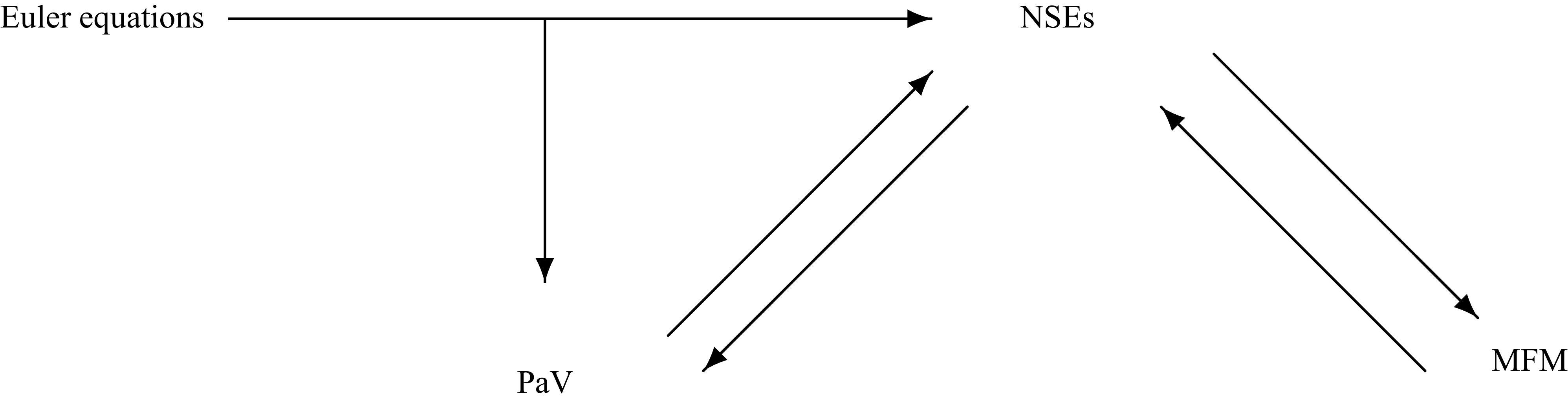

 Open access