


1. Introduction
Order statistics play a significant role in reliability theory, particularly in analyzing the behavior of systems and components with multiple failure modes or components. In reliability theory, order statistics refer to the ordered values of random variables representing failure times or lifetimes of components within a system. The foundational work on order statistics can be attributed to Ronald A. Fisher, who introduced the concept of order statistics in his seminal book [Reference Fisher24]. Assume  $X_1,\dots,X_k,\dots, X_n$ are independent and identically distributed (iid) random variables from a distribution and let $X_{1:n}\leq X_{2:n}\leq\dots X_{k:n}\leq\dots\leq X_{n:n}$ denote the order statistics based on the above random sample. For essential references offering valuable insights into the theory, properties and applications of order statistics, the readers are referred to [Reference Kendall and Stuart30], [Reference Balakrishnan and Rao10], [Reference David and Nagaraja20], [Reference Johnson, Kemp and Kotz28], [Reference Arnold, Balakrishnan and Nagaraja4], [Reference Balakrishnan and Zhao11] etc. In reliability engineering, order statistics represent the observed failure times of components in a system. For instance, the first-order statistic $X_{1:n}$ corresponds to the earliest failure time observed, while the $k$-th order statistic represents the time of the $k$-th failure. Thus, $X_{1:n}$ represents the lifetime of a series system with the Xi‘s as components while $X_{n:n}$ represents the lifetime of the corresponding parallely-connected system. More generally, $X_{k:n}$ represents the lifetime of a $(n-k+1)$-out-of- $n$ system. Analyzing order statistics helps in estimating system reliability, identifying critical components and optimizing maintenance strategies.
Order statistics have numerous practical applications across various domains, including reliability engineering, extreme value analysis, statistical inference, queueing theory etc. They are extensively used in reliability engineering to analyze the failure times of components within a system. For example, order statistics can be used to determine the probability of a system failure based on the order of component failures (see [Reference Yang and Alouini54], [Reference Liu, Chen, Zhang and Cao34], [Reference Mathai37], [Reference Rausand and Hoyland43] etc.). Order statistics play a crucial role in extreme value analysis, where they are used to model and predict rare and extreme events. For instance, order statistics can be used to identify the maximum flood level observed over a given period (see, for example, [Reference Stedinger48]). In statistical inference, order statistics help in understanding the central tendency, spread and shape of a distribution, aiding decision-making in research, industry and policy. For applications of order statistics in statistical inference, the reader is referred to the well-known text by [Reference Berger and Casella17]. In finance, order statistics find widespread applications in analyzing distributions of financial variables such as stock prices, asset returns or income levels (see, for example, [Reference Miller39], [Reference Warin and Leiter53] etc.)
Stochastic ordering of order statistics refers to the comparison of ordered values within a sample or population based on their underlying distributions (see [Reference Shaked and Shanthikumar46] for a detailed discussion regarding theoretical foundations, properties and applications of stochastic ordering in diverse fields). It provides a framework for comparing and ranking random variables, distributions and stochastic processes, enabling researchers to make informed decisions and draw meaningful conclusions in different fields of application.
Majorization is a basic tool that is typically used to explore stochastic comparison results between two sets of independent and heterogeneous random variables (see [Reference Marshall, Olkin and Arnold36] for details). The literature in this area is extensive [for instance, see [Reference Majumder, Ghosh and Mitra35], [Reference Fang, Zhu and Balakrishnan23], [Reference Kundu and Chowdhury32], [Reference Jong-Wuu, Hung and Tsai29], [Reference Zhao, Zhang and Qiao55] etc.]. Chain majorization, which is an extension of the concept of majorization, is a valuable tool for establishing ordering results for order statistics where more than one parameter of the concerned distributions is allowed to vary simultaneously. Utilization of majorization and chain majorization for comparison of order statistics has gained increasing interest among researchers during last four decades. [Reference Bartoszewicz15] and [Reference Shaked and Wong47] discuss comparisons concerning maximum and minimum order statistics in the context of life distributions. Many authors have worked in this area focusing on specific distributions including exponential distribution ([Reference Dykstra, Kochar and Rojo21]), extended exponential distribution ([Reference Barmalzan, Ayat, Balakrishnan and Roozegar13]), gamma distribution ([Reference Kochar and Maochao31], [Reference Misra and Misra40], etc.), exponentiated generalized gamma distribution ([Reference Haidari, Najafabadi and Balakrishnan27]), Weibull ([Reference Balakrishnan, Barmalzan and Haidari7]), exponentiated Weibull distribution ([Reference Barmalzan, Najafabadi and Balakrishnan14]), beta ([Reference Torrado and Kochar52]), log-Lindley ([Reference Chowdhury and Kundu19]), Chen distribution ([Reference Bhattacharyya, Khan and Mitra18]), Burr type XII distribution ([Reference Barmalzan, Ayat and Balakrishnan12]), generalized Lehmann distribution ([Reference Sattari, Barmalzan and Balakrishnan45]) etc. Recently, [Reference Torrado51] explored some interesting ordering results in a more general setting.
In the same vein, we focus on the comparison results of extreme order statistics in the context of a very important generalization of the standard Gompertz distribution. The Gompertz distribution, first introduced by [Reference Gompertz25], provides a versatile tool for modeling phenomena characterized by increasing hazard over time, making it applicable across diverse fields ranging from actuarial science and reliability engineering to biology, economics and epidemiology. Specifically, it is used for modeling the age-specific mortality rate, which has given rise to the eponymous law of mortality one encounters in demographic studies. Also this distribution has many real-life applications, as in marketing management for individual-level simulation of customer lifetime value modeling (see [Reference Bemmaor and Glady16]), study of xylem cell development (see [Reference Rossi, Deslauriers and Morin44]), determining path-lengths of self-avoiding walks (SAWs) on random networks in network theory (see [Reference Tishby, Biham and Katzav49]), modeling failure rates of computer codes (see [Reference Ohishi, Okamura and Dohi42]), describing the fermentation characteristics of chemical components in forages (see [Reference Andrej Lavrenčič and Stefanon3]), modeling the growth of the number of individuals infected during the COVID-19 outbreak (see [Reference Asadi, Di Crescenzo, Sajadi and Spina5]), etc. Interestingly, exponential distributions arise as limits of Gompertz distributions. Also, it exhibits positive skewness and has a monotone failure rate. Therefore, generalizing this distribution to provide more flexibility for modeling different situations is natural. The generalized Gompertz distribution (henceforth referred to as GGD), first introduced by [Reference El-Gohary, Alshamrani and Al-Otaibi22], is a three-parameter distribution with cumulative distribution function (cdf)
 \begin{equation}
F(x)= [1-e^{-\mu(e^{cx}-1)}]^\theta,\,\, x \gt 0\,
(\mu ,\, \theta \gt 0, c \gt 0),
\end{equation}
\begin{equation}
F(x)= [1-e^{-\mu(e^{cx}-1)}]^\theta,\,\, x \gt 0\,
(\mu ,\, \theta \gt 0, c \gt 0),
\end{equation} where  $\theta$ is a shape parameter. We say that a random variable (r.v.) $X$ is GGD ( $\mu, c , \theta$) if $X$ has cdf given by (1).
Note that GGD is a proportional reversed hazard rate (PRHR) model since its cdf can be written as  $G^{\theta}(x)$, where $G(x) = 1-e^{-\mu(e^{cx}-1)}$ is a Gompertz cdf. PRHR models have been widely discussed in the works of [Reference Torrado50] and [Reference Navarro, Torrado and del Águila41]. The use of a variety of parametric families of life distributions is typical in diverse fields such as lifetime modeling, data analysis, reliability and medical studies. These include, among others, the exponential distribution (which has a constant failure rate), the Gompertz and generalized exponential distributions (which have monotone failure rates). On the other hand, non-monotonic ageing is frequently observed in real-world situations, where an early “burn-in” phase is followed by a “useful life” phase and ultimately by “a wear-out” phase (see [Reference Alexander2], [Reference Lai, Xie and Murthy33] and [Reference Al-Khedhairi and El-Gohary1], etc.). Bathtub Failure Rate (BFR) distributions are typically used to model such scenarios. GGD includes all the distributions mentioned above as well as bathtub-shaped failure rates as either limiting situations or special cases. The above observations are summarized in Table 1.
List of well-known distributions as special cases of GGD and their Characterization.

Table 1 Long description
The table relates several named lifetime distributions to their cumulative distribution forms, the parameter settings that produce each case, and the resulting failure-rate pattern. For the exponential distribution, choosing the shape parameter at least one with a positive scale parameter gives an increasing failure rate, while the limiting case with the shape parameter equal to one yields a constant failure rate. For the generalized exponential family in the same limiting scale case, a shape parameter below one corresponds to a decreasing failure rate, and a shape parameter above one corresponds to an increasing failure rate. For the Gompertz distribution, using a positive scale parameter with a shape parameter below one produces a bathtub-shaped failure rate. One row notes a Gompertz-related case when the shape parameter equals one but does not provide the parameter choice or failure-rate pattern. Some entries reference external sources for details, so the table is not fully self-contained for those rows.
It should be noted that the Weibull distribution is commonly used in reliability engineering due to its flexibility in modeling different hazard behaviors. While it can accommodate a variety of hazard rate patterns—such as increasing, decreasing, or constant hazards—it does not fully capture the range of changes in hazard rates that the generalized Gompertz distribution (GGD) can. One key limitation of the Weibull distribution is its lack of a dedicated parameter.
In contrast, the generalized Gompertz distribution (GGD) includes parameters that allow for adjustments not only to the shape of the hazard function but also to the timing of the baseline hazard. This makes the GGD particularly valuable in situations where the timing of risk factors is critical, such as in disease relapse or mechanical failures. However, the complexity and data demands can be a drawback of GGD.
Also, the three-parameter gamma and Weibull distributions are widely used for modeling lifetime data and are popular choices among three-parameter distributions. However, they do have certain limitations. For instance, the cdf of the three-parameter gamma distribution lacks a closed-form expression when the shape parameter is not an integer. However, the generalized Gompertz distribution (GGD) has a closed-form cdf, making it more accessible for analysis and facilitating easy simulation through the inverse transform method based on the formula  $X= \frac{1}{c}ln\left(1-\frac{1}{\mu}ln\left(1-U^\frac{1}{\theta}\right)\right)$, where $U\sim U(0,1).$ Similarly, with the three-parameter Weibull distribution, studies have indicated that maximum likelihood estimators (MLEs) for its parameters may not exhibit desirable behavior across all parameter values, even when the location parameter is set to zero. For example, [Reference Bain and Englehardt6] highlighted issues related to the stability of MLEs in the three-parameter Weibull distribution. Moreover, [Reference Meeker and Escobar38] noted that the nice asymptotic properties expected for MLEs do not necessarily hold when estimating the shape parameter. Given these drawbacks, the generalized Gompertz distribution presents a compelling alternative for modeling lifetime data. Its mathematical properties and ease of simulation make it a reasonable choice for researchers and practitioners looking for reliable modeling solutions.
In spite of its widespread applications in many areas, it is worth noting that stochastic comparison results for GGD are noticeably absent in the literature so far. The authors believe that it is worthwhile to concentrate on this particular aspect. In this article, we have exploited multivariate chain majorization techniques to establish ordering results for extreme order statistics of GGD where the parameters are allowed to vary simultaneously.
Our paper is organized as follows. In Section 2, we start out by recapitulating relevant majorization concepts and some useful lemmas which will later be utilized to prove the main theorems. Section 3 deals with our main findings, which include comparison results for extreme order statistics arising from heterogeneous GGD under multivariate chain majorization. It has two subsections. Subsection 3.1 deals with cases when any two of three parameters vary, and Subsection 3.2 looks at the situation where all three parameters vary simultaneously. For each of the cases, we first prove the stochastic comparison results for two observations and then extend the result for  $n$ observations. Also, we have added an application section for real-life illustrations of our results.
2. Notations and definitions
In this section, we review some basic definitions and well-known results relevant to stochastic orderings and majorization concepts. Let  $X$ and $Y$ be non-negative and absolutely continuous random variables with cdfs $F$ and $G$, survival functions $\bar{F}\,(=1-F)$ and $\bar{G}\,(=1-G)$, pdfs $f$ and $g$, hazard rate functions $h_X(=f/\bar{F})$ and $h_Y(=g/\bar{G})$ and reversed hazard rate functions $h_X(=f/F)$ and $h_Y(=g/G)$, respectively. First, we introduce the four basic stochastic orders.
Definition 2.1. We say that  $X$ is smaller than $Y$ in the
(1) usual stochastic order, denoted by $X \leq_{st} Y$, if
$\bar{F}(t)\leq \bar{G}(t)$ or
$F(t)\geq G(t)\,\, \forall\, t.$
$X \leq_{st} Y$, if
$\bar{F}(t)\leq \bar{G}(t)$ or
$F(t)\geq G(t)\,\, \forall\, t.$(2) hazard rate order, denoted by
$X \leq_{hr} Y$, if
$h_X(t)\geq h_Y(t)$ or
$\frac{\bar{G}(t)}{\bar{F}(t)}$ increases in
$t$
$\forall \, t$ for which this ratio is well defined.(3) reversed hazard rate order, denoted by
$X \leq_{rh} Y,$ if
$r_X(t)\leq r_Y(t)$ or
$\frac{G(t)}{F(t)}$ increases in
$t$
$\forall \, t$ for which this ratio is well defined.(4) likelihood ratio order, denoted by
$X \leq_{lr} Y,$ if
$\frac{g(t)}{f(t)}$ increases in
$t$
$\forall \, t$ for which this ratio is well defined.


The following well-known hierarchical relationships hold: $ \qquad\qquad\qquad\qquad\qquad\qquad\,\,\,\,\,\,\,\,\,\,\,\,\,\,\,\,\,\,\,\,\,\,X \leq_{lr} Y \Rightarrow X \leq_{hr} Y$ $\qquad\qquad\qquad\qquad\qquad\qquad\,\,\,\,\,\,\,\,\,\,\,\,\,\,\,\,\,\,\,\,\,\,\,\,\,\,\Downarrow\;\;\;\;\;\;\;\;\;\;\;\;\;\;\;\;\;\;\;\;\;\;\Downarrow$ $ \qquad\qquad\qquad\qquad\qquad\qquad\,\,\,\,\,\,\,\,\,\,\,\,\,\,\,\,\,\,\,\,\,\,X \leq_{rh} Y \Rightarrow X \leq_{st} Y.$
For more detailed discussions on stochastic orderings and applications, readers are referred to [Reference Shaked and Shanthikumar46]. For convenience, we review a few important definitions and lemmas.
Let  $\lbrace x_{(1)}, \dots , x_{(n)} \rbrace$ and $\lbrace x _{[1]}, \dots , x_{[n]} \rbrace$ denote the increasing and decreasing arrangement of the components of the vector $\textbf{x}=(x_1, \dots x_n)$, respectively.
Definition 2.2. The vector  $\textbf{x}$ is said to be majorized by the vector $\textbf{y}$, denoted by $\textbf{x}\preceq^m \textbf{y}$, if $\displaystyle{\sum_{i=1}^{k}x_{(i)} \geq \sum_{i=1}^{k}y_{(i)}}$ for $ k=1, \dots n-1$ and $\displaystyle{\sum_{i=1}^{n}x_{(i)} = \sum_{i=1}^{n}y_{(i)}}$.
Now we present fundamental definitions for multivariate chain majorization. For this, we first define some properties of matrices. A square matrix  ${\Pi}$ is called a permutation matrix if each of its rows and columns has a single unit and all the remaining entries are zero. A square matrix $T_w$ of order $n$ is said to be a $T$-transform matrix if it can be written as $T_w = w I_n + (1-w) {\Pi},$ where $0\leq w \leq 1,$ and ${\Pi}$ is a permutation matrix which interchanges exactly two coordinates. Let $T_{w_1} = {w_1} I_n + (1-{w_1}) {\Pi_1}$ and $T_{w_2} = {w_2} I_n + (1-{w_2}) {\Pi_2}$ be two $T$-transform matrices as above. $T_{w_1}$ and $T_{w_2}$ are said to have the same structure when ${\Pi_1}= {\Pi_2}$. We say that $T_{w_1}$ and $T_{w_2}$ have different structure when ${\Pi_1}$ and ${\Pi_2}$ are different. It is known that the product of a finite number of $T$-transform matrices with the same structure is also a $T$-transform matrix. This property does not necessarily hold for matrices having different structures. Define $M (\mathbf{r}_\mathbf{1}, \mathbf{r}_\mathbf{2},\dots, \mathbf{r}_\mathbf{m};n)$ as the matrix with the first row vector $\mathbf{r}_\mathbf{1}$, second row vector $\mathbf{r}_\mathbf{2}$,…, $m-$th row vector $\mathbf{r}_\mathbf{m}$ and no of columns $n$.
$n$.
Definition 2.3. Consider two matrices  $U_n$ and $V_n$ such that $U_n= M (\mathbf{u}_\mathbf{1}, \mathbf{u}_\mathbf{2},\dots,\mathbf{u}_\mathbf{m};n)$ and $V_n= M (\mathbf{v}_\mathbf{1}, \mathbf{v}_\mathbf{2},\dots, \mathbf{v}_\mathbf{m};n)$. Then
(1)
$U_n$ is said to chain majorize
$V_n$, denoted by
$U_n \gt \gt V_n;$ if there exists a finite set of
$n\times n$
$T$-transform matrices
$T_{w_1},T_{w_2},\dots,T_{w_k}$ such that
$V_n= U_n T_{w_1}T_{w_2}\dots T_{w_k}$.(2)
$U_n$ is said to majorize
$V_n$ denoted by
$U_n \gt V_n$, if there exists an
$n\times n$ doubly stochastic matrix M such that
$V_n= U_n M$.(3)
$U_n$ is said to row majorize
$V_n$, denoted by
$U_n \gt _{row} V_n,$ if
$u_i\geq_{m} v_i$ for
$i=1,2,\dots,m.$


The relationships between the majorization concepts given in Definition 2.3 are as follows:
 \begin{equation*}U_n \gt \gt V_n \Rightarrow \,\,U_n \gt V_n \Rightarrow \,\,U_n \gt _{row} V_n.\end{equation*}
[Reference Marshall, Olkin and Arnold36] is a good reference for exhaustive study.
We now look at some notations and results regarding multivariate chain majorization, which we will use subsequently. We borrow some notations from the paper [Reference Balakrishnan, Nanda and Kayal9] and given below:
 \begin{equation*}P_n:= \{M(\textbf{x},\textbf{y};n)\,:\,x_i \gt 0,\,y_j \gt 0\, and\, (x_i-x_j)(y_i-y_j)\,\leq 0, i,j= 1,2,\dots,n\}.\end{equation*}
 \begin{equation*}Q_n:= \{M(\textbf{x},\textbf{y};n)\,:\,x_i\geq1,\,y_j \gt 0\, and\, (x_i-x_j)(y_i-y_j)\,\leq 0, i,j= 1,2,\dots,n\}.\end{equation*}
 \begin{equation*}R_n:= \{M(\textbf{x},\textbf{y};n)\,:\,x_i \gt 0,\,y_j \gt 0\, and\, (x_i-x_j)(y_i-y_j)\,\geq 0, i,j= 1,2,\dots,n\}.\end{equation*}
Lemma 2.1. A differentiable function  $\Phi\,:\, \mathbb{R}^{+^4}\to \mathbb{R}^+$ satisfies $\Phi(A)\geq(\leq)\, \Phi(B)$ for all A,B such that $A\in P_2,$ or $Q_2$, or $R_2$ and $A \gt \gt B$ iff
(1)
$\Phi(A)=\Phi(A\Pi)$ for all permutation matrices
$\Pi$ and for all
$A\in P_2,$ or
$Q_2$ or
$R_2$ and(2)
$\sum_{i=1}^2 (a_{ik}-a_{ij})[\Phi_{ik}(A)-\Phi_{ij}(A)]\geq(\leq)\, 0$ for all
$j,k=1,2$ and for all
$A\in P_2,$ or
$Q_2$ or
$R_2$ where
$\Phi_{ij}(A)= \frac{\partial \Phi(A)}{\partial a_{ij}}$.


Lemma 2.2. Let the function  $\phi :\mathbb{R}^{+^2}\to \mathbb{R}^+$ be differentiable and the function $\Phi_n\,:\, \mathbb{R}^{+^{2n}}\to \mathbb{R}^+$ be defined as
 \begin{equation*}
\Phi_n(A)= \prod_{i=1}^n \phi(a_{1i},a_{2i}) .
\end{equation*}
\begin{equation*}
\Phi_n(A)= \prod_{i=1}^n \phi(a_{1i},a_{2i}) .
\end{equation*} Assume that  $\Phi_2$ satisfies the conditions of Lemma 2.1, then for $A\in P_n, or\, Q_n,\, or \,R_n$ and $B=A T_{w}$, we have $\Phi_n(A)\geq \Phi_n(B)$, where $T_w$ is a $T$-transform matrix.
For detailed proofs of Lemma 2.1 and Lemma 2.2, see [Reference Balakrishnan, Haidari and Masoumifard8]. The next two lemmas are extensions of the above lemmas. Let us define for  $i,j,k= 1,2,\dots,n$, $S_n= \{M(\textbf{x},\textbf{y},\textbf{z};n)\,:\,x_i \gt 0,\,y_j \gt 0,z_k \gt 0\,and\,x_i\leq(\geq)x_j,\,\,y_i\geq(\leq)y_j,\,\,z_i\geq(\leq)z_j\}, $ $T_n= \{M(\textbf{x},\textbf{y},\textbf{z};n)\,:\,x_i\geq1,\,y_j \gt 0,z_k \gt 0\,and\,x_i\leq(\geq)x_j,\,\,y_i\geq(\leq)y_j,\,\,z_i\geq(\leq)z_j\}.$
Lemma 2.3. A differentiable function  $\Psi\,:\, \mathbb{R}^{+^6}\to \mathbb{R}^+$ satisfies $\Psi(A)\geq(\leq) \Psi(B)$ for all A,B such that $A\in S_2(T_2)$ and $A \gt \gt B$ iff
(1)
$ \Psi(A)=\Psi(A\Pi)$ for all permutation matrices
$\Pi$ and for all
$A\in S_2(T_2)$ and(2)
$\sum_{i=1}^3 (a_{ik}-a_{ij})[\Psi_{ik}(A)-\Psi_{ij}(A)]\geq(\leq)\, 0$ for all
$j,k=1,2$ and for all
$A\in S_2(T_2)$ where
$\Psi_{ij}(A)= \frac{\partial \Psi(A)}{\partial a_{ij}}.$


Lemma 2.4. Let the function  $\psi :\mathbb{R}^{+^3}\to \mathbb{R}^+$ be differentiable and the function $\Psi_n\,:\, \mathbb{R}^{+^{3n}}\to \mathbb{R}^+$ be defined as
 \begin{equation*}
\Psi_n(A)= \prod_{i=1}^n \psi(a_{1i},a_{2i},a_{3i}) .
\end{equation*}
\begin{equation*}
\Psi_n(A)= \prod_{i=1}^n \psi(a_{1i},a_{2i},a_{3i}) .
\end{equation*} Assume that  $\Psi_2$ satisfies the conditions of Lemma 2.3, then for $A\in S_2(T_2)$ and $B=A T_{w}$, we have $\Psi_n(A)\geq \Psi_n(B)$, where $T_w$ is a $T$-transform matrix.
3. The main results
Let  $X_1,X_2,X_3,\dots,X_n$ be independent generalized Gompertz random variables with $X_i\sim$ GGD ( $\mu_i,\theta_i,c_i$).
The cdf of  $X_i$ is given by
 \begin{equation*}F_i(x)={[1-e^{-\mu_i(e^{c_ix}-1)}]}^{\theta_i}\end{equation*}
 and density function is  $f_i(x)=\theta_i\,\mu_i\,c_i\,e^{c_ix}e^ {-\mu_i({c_ix}-1)}{[1-e^{-\mu_i(e^{c_ix}-1)}]}^{\theta_i-1}$, where $\mu_i \gt 0,c_i \gt ,\theta_i \gt 0.$ The survival function is given by
 \begin{equation}\overline{F_i}(x)= 1-F_i(x)= 1-{[1-e^{-\mu_i(e^{c_ix}-1)}]}^{\theta_i}.
\end{equation}
\begin{equation}\overline{F_i}(x)= 1-F_i(x)= 1-{[1-e^{-\mu_i(e^{c_ix}-1)}]}^{\theta_i}.
\end{equation} If  $h_i(x)\,\text{and}\,r_i(x)$ denote, respectively, the hazard rate function and the reversed hazard rate function of $X_i$, one has
 \begin{equation}
h_i(x)=\frac {\theta_i\,\mu_i\,c_i\,e^{c_ix} e^{-\mu_i(e^{c_ix}-1)}{[1-e^{-\mu_i(e^{c_ix}-1)}]^{\theta_i-1}}}{1-[1-e^{-\mu_i(e^{c_ix}-1)}]^{\theta_i}}
\end{equation}
\begin{equation}
h_i(x)=\frac {\theta_i\,\mu_i\,c_i\,e^{c_ix} e^{-\mu_i(e^{c_ix}-1)}{[1-e^{-\mu_i(e^{c_ix}-1)}]^{\theta_i-1}}}{1-[1-e^{-\mu_i(e^{c_ix}-1)}]^{\theta_i}}
\end{equation}and
 \begin{equation}
r_i(x)=\frac{\theta_i\,\mu_i\,c_i\,e^{c_ix} e^{-\mu_i(e^{c_ix}-1)}}{1-e^{-\mu_i(e^{c_ix}-1)}}.
\end{equation}
\begin{equation}
r_i(x)=\frac{\theta_i\,\mu_i\,c_i\,e^{c_ix} e^{-\mu_i(e^{c_ix}-1)}}{1-e^{-\mu_i(e^{c_ix}-1)}}.
\end{equation} Recall that  $X_{1:n}\,\text{and}\,X_{n:n}$ represent the lifetime of the series and parallel systems with $X_1,X_2,\dots,X_n$ as components. The cdf of $X_{1:n}$ is
 \begin{equation}
F_{{X}_{1:n}}(x)= 1-\prod^n_{i=1}\overline{F_i}(x)=1-\prod^n_{i=1}[1-{(1-e^{-\mu_i(e^{c_ix}-1)})}^{\theta_i}], x \gt 0,
\end{equation}
\begin{equation}
F_{{X}_{1:n}}(x)= 1-\prod^n_{i=1}\overline{F_i}(x)=1-\prod^n_{i=1}[1-{(1-e^{-\mu_i(e^{c_ix}-1)})}^{\theta_i}], x \gt 0,
\end{equation}its pdf is
 \begin{equation}
F_{{X}_{1:n}}(x)=\overline{F}_{{X}_{1:n}}(x)\sum^{n}_{i=1}h_i(x)
\end{equation}
\begin{equation}
F_{{X}_{1:n}}(x)=\overline{F}_{{X}_{1:n}}(x)\sum^{n}_{i=1}h_i(x)
\end{equation}and its hazard rate function is given by
 \begin{equation}
h_{{X}_{1:n}}(x)=\sum^n_{i=1}h_i(x).
\end{equation}
\begin{equation}
h_{{X}_{1:n}}(x)=\sum^n_{i=1}h_i(x).
\end{equation} Now the cdf of  $X_{n:n}$ is given by
 \begin{equation}
F_{X_{n:n}}(x)=\prod_{i=1}^n F_i(x)=\prod_{i=1}^n[1-e^{-\mu_i(e^{c_ix}-1)}]^{\theta_i}, x \gt 0,
\end{equation}
\begin{equation}
F_{X_{n:n}}(x)=\prod_{i=1}^n F_i(x)=\prod_{i=1}^n[1-e^{-\mu_i(e^{c_ix}-1)}]^{\theta_i}, x \gt 0,
\end{equation}its pdf is
 \begin{equation}
F_{X_{n:n}}(x)=F_{X_{n:n}}(x)\sum^n_{i=1}r_i(x),
\end{equation}
\begin{equation}
F_{X_{n:n}}(x)=F_{X_{n:n}}(x)\sum^n_{i=1}r_i(x),
\end{equation}and its reversed hazard rate function is given by
 \begin{equation}
r _{X_{n:n}}(x)=\sum^n_{i=1}r_i(x).
\end{equation}
\begin{equation}
r _{X_{n:n}}(x)=\sum^n_{i=1}r_i(x).
\end{equation}3.1. Multivariate chain majorization with heterogeneity in two parameters
Here, we develop comparison results focusing on multivariate chain majorization between two sets of generalized Gompertz distribution having heterogeneity in two parameters. In order to investigate stochastic comparison under chain majorization with respect to  $(\boldsymbol{c},\boldsymbol{\mu}),$ we shall first require the following three lemmas. The first two are due to [Reference Balakrishnan, Haidari and Masoumifard8] and the next one is our own contribution.
Lemma 3.1. Consider the function  $\psi_5: (0,\infty) \times (0,1)\to (0,\infty)$ defined by
 \begin{equation}
\psi_5(\beta, t) = \dfrac{\beta(1-t)t^{\beta-1}}{1-t^\beta}.
\end{equation}
\begin{equation}
\psi_5(\beta, t) = \dfrac{\beta(1-t)t^{\beta-1}}{1-t^\beta}.
\end{equation}Then
(1)
$\psi_5(\beta, t)$ is decreasing with respect to
$\beta$ for all
$0 \lt t \lt 1.$(2)
$\psi_5(\beta, t)$ is decreasing with respect to
$t $ for all
$0 \lt \beta\leq1.$(3)
$\psi_5(\beta, t)$ is increasing with respect to
$t$ for all
$\beta\geq 1.$


Lemma 3.2. Consider the function  $\psi_6: (0,\infty) \times (0,1)\to (0,\infty)$ defined by
 \begin{equation}
\psi_6(\beta, t)= \dfrac{t^\beta\log t}{1-t^\beta}.
\end{equation}
\begin{equation}
\psi_6(\beta, t)= \dfrac{t^\beta\log t}{1-t^\beta}.
\end{equation}Then
(1)
$ \psi_6(\beta, t)$ is increasing with respect to
$\beta$ for all
$0 \lt t \lt 1$.(2)
$ \psi_6(\beta, t)$ is decreasing with respect to
$t$ for all
$\beta \gt 0$.


For detailed proof of the Lemma 3.1 and Lemma 3.2, see [Reference Balakrishnan, Haidari and Masoumifard8].
Lemma 3.3. For  $\lambda \gt 0,$ the function $\psi_2^{(\lambda)}(x)=\dfrac{x}{e^{\lambda x}-1}, x \gt 0$ is decreasing and convex in $x$.
$x$.
Proof. Differentiating  $\psi_2^{(\lambda)}(x)$ with respect to $x$ we get $\psi_2^{(\lambda)\prime}(x) \overset{\textsf{sign}}= e^{\lambda x}-1-x\lambda e^{\lambda x}= v_1^{(\lambda)}(x)$, say. $v_1^{(\lambda)}(x)$ is a decreasing function in $x$ as $v_1^{(\lambda)\prime}(x)=-\lambda^2x e^{\lambda x} \lt 0.$ Also $\lim_{x\to 0^+}v_1^{(\lambda)}(x)=0$ leads to the fact that $v_1^{(\lambda)}(x) \lt 0$ and this implies $ \psi_2^{(\lambda)}(x) $ is a decreasing function in $x$
$x$  $\forall \lambda \gt 0.$
Now we differentiate  $ \psi_2^{(\lambda)\prime}(x)$ with respect to $x$ and get $\psi_2^{(\lambda)\prime\prime}(x) \overset{\textsf{sign}}= \lambda x e^{\lambda x}+\lambda x+2-2e^{\lambda x}= v_2^{(\lambda)}(x)$, say.
Using the inequality  $e^{-\lambda x} \gt 1-\lambda x$ it can be shown that $v_2^{(\lambda)}(x)$ is increasing in $x$. Again $\lim_{x\to 0^+}v_2^{(\lambda)}(x)=0$ leads to the conclusion that $v_2^{(\lambda)}(x)$ is greater than zero, i.e., $\psi_2^{(\lambda)\prime\prime}(x) \gt 0$. This establishes the convexity.
Proposition 3.1. Let  $X_1,X_2$ be independent random variables with $X_i\sim GGD(\mu_i,c_i,\theta),\, i=1,2.$ Also let $X_1^*,X_2^*$ be independent random variables with $X_i\sim GGD(\mu_i^*,c_i^*,\theta),\, i=1,2.$ If $M(\boldsymbol{\mu},\boldsymbol{c};2)\in R_2$ and $M(\boldsymbol{\mu},\boldsymbol{c};2) \gt \gt M(\boldsymbol{\mu^*},\boldsymbol{c^*};2)$, we have
(i)
$X_{2:2}\geq_{st}X_{2:2}^*$(ii)
$X_{1:2}\leq_{st}X_{1:2}^*$ when
$\theta\geq 1$


(1) The distribution function of
$X_{2:2}$ is given by
(13)\begin{equation}
F_{X_{2:2}}(x) =\prod\limits_{i=1}^2{(1-e^{-\mu_i(e^{c_ix}-1)})}^\theta.
\end{equation}Condition (i) of Lemma 2.1 is satisfied as
$ F_{X_{2:2}}(x)$ is permutation invariant in
$(\boldsymbol{\mu},\boldsymbol{c})$. Thus, to prove the theorem, it suffices to verify condition (ii) of Lemma 2.1. For fixed
$x \gt 0$, let us define the function
$\zeta_1(\boldsymbol{\mu},\boldsymbol{c})$ as follows:
\begin{equation*}\zeta_1(\boldsymbol{\mu},\boldsymbol{c})= \zeta_1^{(1)}(\boldsymbol{\mu},\boldsymbol{c}) + \zeta_1^{(2)}(\boldsymbol{\mu},\boldsymbol{c})\end{equation*}where
\begin{equation*}\zeta_1^{(1)}(\boldsymbol{\mu},\boldsymbol{c})= (\mu_1-\mu_2)\left(\frac{\partial F_{X_{2:2}}(x)}{\partial \mu_1}-\frac{\partial F_{X_{2:2}}(x)}{\partial\mu_2} \right)\end{equation*}and
\begin{equation*}\zeta_1^{(2)}(\boldsymbol{\mu},\boldsymbol{c})= (c_1-c_2)\left(\frac{\partial F_{X_{2:2}}(x)}{\partial c_1}-\frac{\partial F_{X_{2:2}}(x)}{\partial c_2} \right).\end{equation*}Differentiating
$F_{X_{2:2}}(x)$ partially with respect to
$\mu_i$ and
$c_i$ we get the following expressions:
\begin{equation*}\frac{\partial F_{X_{2:2}}(x)}{\partial \mu_i}= F_{X_{2:2}}(x)\frac{\theta}{\mu_i}\psi_2^{(1)}\left(\mu_i(e^{c_ix}-1)\right)\end{equation*}and
\begin{equation*}\frac{\partial F_{X_{2:2}}(x)}{\partial c_i}=\theta x F_{X_{2:2}}(x) \psi_2^{(1)}\left(\mu_i(e^{c_ix}-1)\right)\delta(e^{c_ix}) \end{equation*}where
$\psi_2^{(1)}(x)$ is defined in Lemma 3.3 for the special case of
$\lambda =1$ and
$\delta(x)$ is defined by
$\delta(x)= \frac{x}{x-1},\,x \gt 0 .$ From Lemma 3.3 it is known that
$\psi_2^{(1)}(x)$ is decreasing with respect to
$x$ and clearly it can be noted that
$\delta(x)$ is decreasing with respect to
$x$. Now for
$M(\boldsymbol{\mu},\boldsymbol{c};2)\in R_2$ following two cases may arise:(i) Case 1:
$\mu_1,\mu_2,c_1,c_2 \gt 0$ and
$\mu_1\geq\mu_2;\, c_1\geq c_2.$(ii) Case 2:
$\mu_1,\mu_2,c_1,c_2 \gt 0$ and
$\mu_1\leq\mu_2;\, c_1\leq c_2.$
Under Case 1 [Case 2], we have
\begin{equation*}\left(\mu_1(e^{c_1x}-1)\right)\geq[\leq]\left(\mu_2(e^{c_2x}-1)\right).\end{equation*}As
$\psi_2^{(1)}(x)$ and
$\delta(x)$ are decreasing with respect to
$x$ we have for both cases
$\zeta_1^{(1)}(\boldsymbol{\mu},\boldsymbol{c})\leq 0$ and
$\zeta_2^{(1)}(\boldsymbol{\mu},\boldsymbol{c})\leq 0$. Consequently, condition (ii) of Lemma 2.1 is satisfied, and thus the proof is completed by applying Definition 2.1.(2) The survival function of
$X_{1:2}$ is given by
(14)\begin{equation}
\overline{F}_{X_{1:2}}(x)=\prod\limits_{i=1}^2[1-{(1-e^{-\mu_i(e^{c_ix}-1)})}^\theta].
\end{equation}Here,
$\overline{F}_{X_{1:2}}(x)$ is permutation invariant in
$(\boldsymbol{\mu},\boldsymbol{c})$. So we need to establish only condition (ii) of Lemma 2.1. Consider the function
$\zeta_2(\boldsymbol{\mu},\boldsymbol{c})$ as following:
\begin{equation*}\zeta_2(\boldsymbol{\mu},\boldsymbol{c})=(\mu_1-\mu_2)\left(\frac{\partial \overline{F}_{X_{1:2}}}{\partial \mu_1}-\frac{\partial \overline{F}_{X_{1:2}}}{\partial\mu_2} \right)+ (c_1-c_2)\left(\frac{\partial\overline{F}_{X_{1:2}}}{\partial c_1}-\frac{\partial\overline{F}_{X_{1:2}}}{\partial c_2} \right).\end{equation*}Now differentiating
$\overline{F}_{X_{1:2}}(x)$ partially with respect to
$\mu_i$ and
$c_i$ we have
(15)\begin{align}
& \frac{\partial\overline{F}_{X_{1:2}}(x)}{\partial\mu_i}= -\overline{F}_{X_{1:2}}(x)\,(e^{c_ix}-1)\,\psi_5(\theta,1-e^{-\mu_i(e^{c_ix}-1)})\,\, and \nonumber \\ & \frac{\partial\overline{F}_{X_{1:2}}(x)}{\partial c_i}= -\overline{F}_{X_{1:2}}(x)(x) x\mu_i e^{c_ix}\,\psi_5(\theta,1-e^{-\mu_i(e^{c_ix}-1)}),
\end{align}where
$\psi_5(\beta,t):(0,\infty)\times(0,1)$ is defined in Lemma 3.1. So
$\zeta_2(\boldsymbol{\mu},\boldsymbol{c})$ becomes
\begin{align*}
\zeta_2(\boldsymbol{\mu},\boldsymbol{c})&= -\overline{F}_{X_{1:2}}(x)(\mu_1-\mu_2)[(e^{c_1x}-1)\,\psi_5(\theta,1-e^{-\mu_1(e^{c_1x}-1)})-(e^{c_2x}-1)\,\nonumber \\ & \qquad \quad \psi_5(\theta,1-e^{-\mu_2(e^{c_2 x}-1)})]\\ & -\overline{F}_{X_{1:2}}(x)x(c_1-c_2)[\mu_1 e^{c_1 x}\,\psi_5(\theta,1-e^{-\mu_1(e^{c_1 x}-1)})-\mu_2 e^{c_2 x}\,\psi_5(\theta,1-e^{-\mu_2(e^{c_2 x}-1)})].
\end{align*}Again for
$M(\boldsymbol{\mu},\boldsymbol{c};2)\in R_2$, two cases may be possible which are given in part (i). Now by the Lemma 3.1, under Case(i)[Case (ii)] we have
\begin{equation*}\psi_5(\theta,1-e^{-\mu_1(e^{c_1x}-1)}) \geq[\leq] \psi_5(\theta,1-e^{-\mu_2(e^{c_2x}-1)})\,\,\text{for}\,\, \theta\geq 1,\end{equation*}since
$\psi_5(\beta,t)$ is increasing in
$t$ for all
$\theta\geq 1$. After some basic algebraic manipulation, it can be proved that
$\zeta_2(\boldsymbol{\mu},\boldsymbol{c})\leq 0$ in either of the cases. Therefore, condition (ii) of Lemma 2.1 is satisfied and this completes the proof.


We now generalize Proposition 3.1 for  $n \gt 2$ by using Lemma 2.2.
Theorem 3.1. Let  $X_1,X_2,\dots X_n$ be independent random variables with $X_i\sim GGD(\mu_i,c_i,\theta),\, i=1,2,\dots,n.$ Also let $X_1^*,X_2^*\dots,X_n^*$ be independent random variables with $X_i\sim GGD(\mu_i^*,c_i^*,\theta),\, i=1,2,\dots,n.$ If $M(\boldsymbol{\mu},\boldsymbol{c};n)\in R_n$ and $M(\boldsymbol{\mu^*},\boldsymbol{c^*};n)= M(\boldsymbol{\mu},\boldsymbol{c};n) T_w$, we have
(i)
$X_{n:n}\geq_{st}X_{n:n}^*$(ii)
$X_{1:n}\leq_{st}X_{1:n}^*$ when
$\theta\geq 1$


(i) If
$M(\boldsymbol{\mu},\boldsymbol{c};n)\in R_n$ and
$M(\boldsymbol{\mu^*},\boldsymbol{c^*};n)= M(\boldsymbol{\mu},\boldsymbol{c};n) T_w$, suppose that
\begin{equation*}\Psi_n(\boldsymbol{\mu},\boldsymbol{c},\theta)= \prod\limits_{i=1}^n{(1-e^{-\mu_i(e^{c_i x}-1)})}^\theta = F_{X_{n:n}}(x).\end{equation*}Let us denote
$\psi(\mu_i,c_i)= {(1-e^{-\mu_i(e^{c_i x}-1)})}^\theta$,
$i=1,2,\dots,n.$ Using Proposition 3.1, we can observe that under the assumption of this theorem,
$\Psi_2(\boldsymbol{\mu},\boldsymbol{c},\theta)$ satisfies all the conditions of Lemma 2.2 and hence can be proved by Lemma 2.2.(ii) The proof is similar to that of (i).


The following corollary is immediate.
Corollary 3.1. Let  $X_1,X_2,\dots X_n$ be independent random variables with $X_i\sim GGD(\mu_i,c_i,\theta),\, i=1,2,\dots,n.$ Also let $X_1^*,X_2^*\dots,X_n^*$ be independent random variables with $X_i\sim GGD(\mu_i^*,c_i^*,\theta),\, i=1,2,\dots,n.$ If $M(\boldsymbol{\mu},\boldsymbol{c};n)\in R_n$ and $M(\boldsymbol{\mu^*},\boldsymbol{c^*};n)= M(\boldsymbol{\mu},\boldsymbol{c};n) T_{w_1}T_{w_2}\dots T_{w_k}$ where $T_{w_1},T_{w_2},\dots,T_{w_k}$ have the same structure, we have
(i)
$X_{n:n}\geq_{st}X_{n:n}^*$(ii)
$X_{1:n}\leq_{st}X_{1:n}^*$ when
$\theta\geq 1$


To illustrate the result in (i) of Theorem 3.1, we now present the following numerical example.
Example 3.1. Let  $X_i$ and $X_i^*$ be independent random variables such that $X_i\sim GGD(\mu_i,c_i,\theta)$ and $X_i^*\sim GGD(\mu^*_i,c^*_i,\theta),$ i=1,2.
We fix  $\theta=0.05$ and set
 \begin{equation*}
M(\boldsymbol{\mu},\boldsymbol{c};2)= \begin{bmatrix}
\mu_1&\mu_2\\c_1&c_2
\end{bmatrix}=\begin{bmatrix}
0.1&0.05\\0.4&0.2
\end{bmatrix}
\,\,\text{and}\,\, M(\boldsymbol{\mu^*},\boldsymbol{c^*};2)= \begin{bmatrix}
\mu^*_1&\mu^*_2\\c^*_1&c^*_2
\end{bmatrix}=\begin{bmatrix}
0.07&0.08\\0.28&0.32
\end{bmatrix}.
\end{equation*}
\begin{equation*}
M(\boldsymbol{\mu},\boldsymbol{c};2)= \begin{bmatrix}
\mu_1&\mu_2\\c_1&c_2
\end{bmatrix}=\begin{bmatrix}
0.1&0.05\\0.4&0.2
\end{bmatrix}
\,\,\text{and}\,\, M(\boldsymbol{\mu^*},\boldsymbol{c^*};2)= \begin{bmatrix}
\mu^*_1&\mu^*_2\\c^*_1&c^*_2
\end{bmatrix}=\begin{bmatrix}
0.07&0.08\\0.28&0.32
\end{bmatrix}.
\end{equation*} It is easy to note that  $ M(\boldsymbol{\mu},\boldsymbol{c};2)\in R_2.$ We now consider a $T$-transform matrix
  $T_{0.4}=\begin{bmatrix}
0.4&0.6\\0.6&0.4
\end{bmatrix}$, so that
$T_{0.4}=\begin{bmatrix}
0.4&0.6\\0.6&0.4
\end{bmatrix}$, so that
 \begin{equation*}
\begin{bmatrix}
0.07&0.08\\0.28&0.32
\end{bmatrix}= \begin{bmatrix}
0.1&0.05\\0.4&0.2
\end{bmatrix} \times \begin{bmatrix}
0.4&0.6\\0.6&0.4
\end{bmatrix}.
\end{equation*}
\begin{equation*}
\begin{bmatrix}
0.07&0.08\\0.28&0.32
\end{bmatrix}= \begin{bmatrix}
0.1&0.05\\0.4&0.2
\end{bmatrix} \times \begin{bmatrix}
0.4&0.6\\0.6&0.4
\end{bmatrix}.
\end{equation*} Now from Definition 2.3,  $M(\boldsymbol{\mu},\boldsymbol{c};2) \gt \gt M(\boldsymbol{\mu^*},\boldsymbol{c^*};2).$ Let
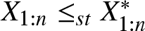
  $F_X(x)$ and $F_Y(x)$ denote the cdfs of $X_{2:2}$ and $X^*_{2:2}$, respectively.
Now from Figure 1, it is evident that  $X_{2:2}\geq_{st}X_{2:2}^*,$ which illustrates the result in (i) of Theorem 3.1.
Plot of  ${F_X(x)} \,\text{and}\, {F_Y(x)}$

Figure 1 Long description
The x-axis has tick labels 20, 40, 60, 80 and 100, spanning 0 to 100. The y-axis has tick labels 0.80, 0.85, 0.90, 0.95 and 1.00, spanning 0.80 to 1.00. The axis labels and units are not shown. Two lines are labeled in the legend as F subscript Y and F subscript X. Both lines rise as x increases and approach 1.00. At x equals 20, F subscript Y is slightly below 0.90 and F subscript X is slightly below F subscript Y. At x equals 40, F subscript Y is between 0.90 and 0.95 and F subscript X is slightly lower. At x equals 60, F subscript Y is between 0.95 and 1.00 and F subscript X is slightly lower. At x equals 80, both lines are between 0.95 and 1.00, with F subscript Y higher than F subscript X. At x equals 100, both lines are close to 1.00, with F subscript Y higher than F subscript X.
A natural question that arises in this context is whether we can strengthen the conclusion in (i) of Theorem 3.1 to hazard rate order or reversed hazard rate order or likelihood ratio order. The following example demonstrates that no such strengthening is possible.
Example 3.2. Let  $X_i$ and $X_i^*$ be independent random variables such that $X_i\sim GGD(\mu_i,c_i,\theta)$ and $X_i^*\sim GGD(\mu^*_i,c^*_i,\theta),$ i=1,2.
Let us choose same  $\theta,$ $ M(\boldsymbol{\mu},\boldsymbol{c};2)$ and $M(\boldsymbol{\mu^*},\boldsymbol{c^*};2)$ as in Example 3.1. Clearly, all the conditions of Theorem 3.1 are satisfied. Now we plot $\dfrac{{F}_{X_{2:2}}}{{F}_{X^*_{2:2}}}$ and $\dfrac{\overline{F}_{X_{2:2}}}{\overline{F}_{X^*_{2:2}}}$ in Figures 2 and 3, respectively.
Plot of  $\dfrac{F_{X_{2:2}}(x)}{F_{X^*_{2:2}}(x)}$

Figure 2 Long description
The x-axis represents values from 0 to 10, with labeled ticks at 2, 4, 6, 8 and 10. The y-axis represents the ratio of F subscript X subscript 2 colon 2 over F subscript X superscript asterisk subscript 2 colon 2, ranging from 0.92 to 1.04, with labeled ticks at 0.92, 0.94, 0.96, 0.98, 1.00, 1.02 and 1.04. A single solid line is plotted throughout. From x equals 0 to approximately x equals 2, the line holds near y equals 0.99, remaining just below 1.00. Between x equals 2 and approximately x equals 2.5, the line drops sharply, falling toward y equals 0.92. The line reaches its minimum value of approximately 0.92 near x equals 2.5. The line is not visible between approximately x equals 2.5 and x equals 5.2, indicating a region where values fall outside the plotted y-axis range. The line reappears near x equals 5.2 at approximately y equals 0.92. From x equals 5.2 onward, the line rises gradually: near y equals 0.96 at x equals 6, near y equals 0.97 at x equals 7, near y equals 0.975 at x equals 8, near y equals 0.978 at x equals 9 and approaching y equals 0.98 at x equals 10. The highest y-axis tick of 1.04 has no plotted values near it. The overall pattern shows the ratio near 1.00 at low x values, a sharp decline to a minimum near 0.92, followed by a gradual recovery toward 0.98 as x increases to 10.
Plot of  $\dfrac{\overline{F}_{X_{2:2}}(x)}{\overline{F}_{X^*_{2:2}}(x)}$

Figure 3 Long description
A line graph with a single solid line. The x-axis ranges from 0 to 100 with tick marks at 20, 40, 60, 80 and 100. The y-axis ranges from 1.0 to 2.0 with tick marks at 1.2, 1.4, 1.6, 1.8 and 2.0. Both axes are not labeled and no units are provided. The line begins near y equals 1.8 at a low x value close to 0, then drops sharply to a minimum of approximately y equals 1.1 near x equals 10. After this trough, the line rises smoothly and continuously, passing near y equals 1.2 around x equals 30, y equals 1.4 around x equals 55, y equals 1.6 around x equals 75 and y equals 1.8 around x equals 90, reaching just above y equals 2.0 at x equals 100. There are no additional data series, markers, or legends present.
From Figure 2, we see that  $\dfrac{F_{X_{2:2}}(x)}{F_{X^*_{2:2}}(x)}$ is nonmonotonic. So from Definition 2.1 we have $X_{2:2}\ngeq_{rh} X^*_{2:2}.$ From Figure 3, it is evident that $\dfrac{\overline{F}_{X_{2:2}}(x)}{\overline{F}_{X^*_{2:2}}(x)}$ is also nonmonotonic. Hence from Definition 2.1 we have $X_{2:2}\ngeq_{hr} X^*_{2:2}$. Also from the inter relationship of orderings we have $X_{2:2}\ngeq_{lr} X^*_{2:2}.$
We now provide the following numerical example that illustrates the result in (ii) of Theorem 3.1.
Example 3.3. Let  $X_i$ and $X_i^*$ be independent random variables such that $X_i\sim GGD(\mu_i,c_i,\theta)$ and $X_i^*\sim GGD(\mu^*_i,c^*_i,\theta),$ i=1,2.
Let us fix  $\theta=2$ and consider $ M(\boldsymbol{\mu},\boldsymbol{c};2)$ and $M(\boldsymbol{\mu^*},\boldsymbol{c^*};2)$ as in Example 3.1. Consequently, $M(\boldsymbol{\mu},\boldsymbol{c};2) \gt \gt M(\boldsymbol{\mu^*},\boldsymbol{c^*};2).$ Let $X$ and $Y$ represent the random variables $X_{1:2}$ and $X^*_{1:2}$, respectively. We now plot survival functions $\overline{F}_{X}(x)$ and $\overline{F}_{Y}(x)$ in Figure 4. It can be noted that $\overline{F}_{X}$ is dominated by $\overline{F}_{Y}$ which clearly shows that $X_{1:2}\leq_{st}X_{1:2}^*$.
Plot of  $\overline{F}_{X}(x)\,\text{and}\,{\overline{F}_{Y}(x)}$

Figure 4 Long description
Text on the graphic: F bar subscript Y. F bar subscript X. Axes and scales: The horizontal axis label is not shown and the unit is not shown. The horizontal tick labels shown are 20, 40, 60, 80, 100, giving a shown range from 20 to 100. The vertical axis label is not shown and the unit is not shown. The vertical tick labels shown are 0.2, 0.4, 0.6, 0.8, 1.0, giving a shown range from 0.2 to 1.0. Line identification and styling: Two smooth curves are shown. The curve labeled F bar subscript Y is drawn with a thicker line than the curve labeled F bar subscript X. Each label is connected to its curve by a leader line near the right side of the plot. Plotted values (no point markers; values listed only where the curves align with labeled ticks): F bar subscript Y: (20, 0.8), (40, 0.4), (60, 0.2) F bar subscript X: (20, 0.6), (40, 0.3), (60, 0.2) Trends and comparisons: Both curves decrease from left to right. F bar subscript Y is higher than F bar subscript X at x equals 20 and x equals 40. The two curves meet at x equals 60 with y equals 0.2. Both curves continue downward toward the right edge near x equals 100, ending close to the bottom of the plot area.
In the following example, we shall examine whether the findings of (ii) of Theorem 3.1 can be further strengthened.
Example 3.4. Let  $X_i$ and $X_i^*$ be independent random variables such that $X_i\sim GGD(\mu_i,c_i,\theta)$ and $X_i\sim GGD(\mu^*_i,c^*_i,\theta),$ i=1,2.
We consider  $\theta=2$ and set
 \begin{equation*}
M(\boldsymbol{\mu},\boldsymbol{c};2)=\begin{bmatrix}
0.4&0.2\\0.6&0.1
\end{bmatrix}
\,\,\text{and}\,\, M(\boldsymbol{\mu^*},\boldsymbol{c^*};2)=\begin{bmatrix}
0.24&0.36\\0.20&0.50
\end{bmatrix}.
\end{equation*}
\begin{equation*}
M(\boldsymbol{\mu},\boldsymbol{c};2)=\begin{bmatrix}
0.4&0.2\\0.6&0.1
\end{bmatrix}
\,\,\text{and}\,\, M(\boldsymbol{\mu^*},\boldsymbol{c^*};2)=\begin{bmatrix}
0.24&0.36\\0.20&0.50
\end{bmatrix}.
\end{equation*} Clearly,  $ M(\boldsymbol{\mu},\boldsymbol{c};2)\in R_2.$ Let us choose a $T$-transform matrix
  $T_{0.2}=\begin{bmatrix}
0.2&0.8\\0.8&0.2
\end{bmatrix}$, such that
$T_{0.2}=\begin{bmatrix}
0.2&0.8\\0.8&0.2
\end{bmatrix}$, such that
 \begin{equation*}
\begin{bmatrix}
0.24&0.36\\0.20&0.50
\end{bmatrix}= \begin{bmatrix}
0.4&0.2\\0.6&0.1
\end{bmatrix} \times \begin{bmatrix}
0.2&0.8\\0.8&0.2
\end{bmatrix}.
\end{equation*}
\begin{equation*}
\begin{bmatrix}
0.24&0.36\\0.20&0.50
\end{bmatrix}= \begin{bmatrix}
0.4&0.2\\0.6&0.1
\end{bmatrix} \times \begin{bmatrix}
0.2&0.8\\0.8&0.2
\end{bmatrix}.
\end{equation*} Using Definition 2.3 it is easy to observe that  $M(\boldsymbol{\mu},\boldsymbol{c};2) \gt \gt M(\boldsymbol{\mu^*},\boldsymbol{c^*};2).$ Now we plot $\dfrac{{F}_{X^*_{1:2}}(x)}{{F}_{X_{1:2}}(x)}$ in Figure 5 and see that $\dfrac{{F}_{X^*_{1:2}}(x)}{{F}_{X_{1:2}}(x)}$ is nonmonotonic. Consequently, $X_{1:2}\nleq_{rh}X^*_{1:2}$ and also from the interrelationship we have $X_{1:2}\nleq_{lr}X^*_{1:2}$.
Plot of  $\dfrac{{F}_{X^*_{1:2}}(x)}{{F}_{X_{1:2}}(x)}$

However, we are unable to neither prove nor disprove the validity of hazard rate ordering between  $X_{1:n}$ and $Y_{1:n}$ in this case. This problem remains open.
Here is an interesting situation when the  $T_{w_i}$’s, $i=1,2,\dots,n$, do not have the same structure. In this case, one has the following result.
Theorem 3.2. Let  $X_1,X_2,\dots X_n$ be independent random variables with $X_i\sim GGD(\mu_i,c_i,\theta),\, i=1,2,\dots,n.$ Also let $X_1^*,X_2^*\dots,X_n^*$ be independent random variables with $X_i\sim GGD(\mu_i^*,c_i^*,\theta),\, i=1,2,\dots,n.$ If $M(\boldsymbol{\mu},\boldsymbol{c};n)\in R_n$ and $M(\boldsymbol{\mu},\boldsymbol{c};n)T_{w_1}T_{w_2}\dots T_{w_i}\in R_n$ for i=1,2,…,k; $k\geq1$. If $M(\boldsymbol{\mu^*},\boldsymbol{c^*};n)= M(\boldsymbol{\mu},\boldsymbol{c};n) T_{w_1}T_{w_2}\dots T_{w_k}$, then we have
(i)
$X_{n:n}\geq_{st}X_{n:n}^*$(ii)
$X_{1:n}\leq_{st}X_{1:n}^*$ when
$\theta\geq 1$


(i)
$M(\boldsymbol{\mu^{(i)}},\boldsymbol{c^{(i)}};n) = M(\boldsymbol{\mu},\boldsymbol{c};n)T_{w_1}T_{w_2}\dots T_{w_i}$, where
$\boldsymbol{\mu^{(i)}}= (\mu_1^{(i)},\mu_2^{(i)},\dots,\mu_n^{(i)})$ and
$\boldsymbol{c^{(i)}}= (c_1^{(i)},c_2^{(i)},\dots,c_n^{(i)});\,\,$
$i=1,2,\dots,k.$ In addition, let
$Z_1^{(i)},Z_2^{(i)},\dots Z_n^{(i)}$ be independent random variables with
$Z_j^{(i)} = GGD(\mu_j^{(i)},c_j^{(i)},\theta)$, where
$j=1,2,\dots,n$ and
$i=1,2,\dots, k.$ If
$M(\boldsymbol{\mu},\boldsymbol{c};n)\in R_n$, then from the assumption of the theorem,
$M(\boldsymbol{\mu^{(i)}},\boldsymbol{c^{(i)}};n)\in R_n$,
$i=1,2,\dots,k.$Now
$M(\boldsymbol{\mu^*},\boldsymbol{c^*};n)=\{M(\boldsymbol{\mu},\boldsymbol{c};n) T_{w_1},T_{w_2},\dots,T_{w_{k-1}}\}T_{w_k}= M(\boldsymbol{\mu^{(k-1)}},\boldsymbol{c^{(k-1)}};n) T_{w_k}$. Now from Theorem 3.1, we have
$Z_{n:n}^{(k-1)}\geq_{st} X^*_{n:n}.$ Again
$M(\boldsymbol{\mu^{(k-1)}},\boldsymbol{c^{(k-1)}};n)= \{M(\boldsymbol{\mu},\boldsymbol{c};n) T_{w_1},T_{w_2},\dots,T_{w_{k-2}}\}T_{w_{k-1}}= M(\boldsymbol{\mu^{(k-2)}},\boldsymbol{c^{(k-2)}};n) T_{w_{k-1}}$. This gives
$Z_{n:n}^{(k-2)}\geq_{st} Z_{n:n}^{(k-1)}$. Proceeding in a similar manner, we get the sequence
\begin{equation*}X_{n:n}\geq_{st}Z_{n:n}^{(1)}\geq_{st}\dots\geq_{st}Z_{n:n}^{(k-2)}\geq_{st}Z^{(k-1)}_{n:n}\geq_{st}X_{n:n}^*.\end{equation*}This completes the proof.
(ii) The proof is similar to (i).


The following example validates the results in Theorem 3.2.
Example 3.5. Let  $X_i$ and $X_i^*$ be independent random variables such that $X_i\sim GGD(\mu_i,c_i,\theta)$ and $X_i\sim GGD(\mu^*_i,c^*_i,\theta),$ i=1,2,3.
We consider  $\theta=1.2$ and set
 \begin{equation*}
M(\boldsymbol{\mu},\boldsymbol{c};3)=\begin{bmatrix}
0.1&0.2&0.3\\0.2&0.5&0.8
\end{bmatrix}
\,\,\text{and}\,\, M(\boldsymbol{\mu^*},\boldsymbol{c^*};3)=\begin{bmatrix}
0.18&0.192&0.228\\0.44&0.476&0.584
\end{bmatrix}.
\end{equation*}
\begin{equation*}
M(\boldsymbol{\mu},\boldsymbol{c};3)=\begin{bmatrix}
0.1&0.2&0.3\\0.2&0.5&0.8
\end{bmatrix}
\,\,\text{and}\,\, M(\boldsymbol{\mu^*},\boldsymbol{c^*};3)=\begin{bmatrix}
0.18&0.192&0.228\\0.44&0.476&0.584
\end{bmatrix}.
\end{equation*} Clearly,  $M(\boldsymbol{\mu^*},\boldsymbol{c^*};3)\in R_3.$ We now consider two $T-$ transform matrices
 \begin{equation*}
T_{0.2}=\begin{bmatrix}
0.2&0.8&0\\0.8&0.2&0\\0&0&1
\end{bmatrix}
\,\,\text{and}\,\, T_{0.6}=\begin{bmatrix}
1&0&0\\0&0.6&0.4\\0&0.4&0.6
\end{bmatrix}.
\end{equation*}
\begin{equation*}
T_{0.2}=\begin{bmatrix}
0.2&0.8&0\\0.8&0.2&0\\0&0&1
\end{bmatrix}
\,\,\text{and}\,\, T_{0.6}=\begin{bmatrix}
1&0&0\\0&0.6&0.4\\0&0.4&0.6
\end{bmatrix}.
\end{equation*} such that  $M(\boldsymbol{\mu^*},\boldsymbol{c^*};3)=M(\boldsymbol{\mu},\boldsymbol{c};3) T_{0.2}T_{0.6}.$ It is easy to verify that the two $T-$ transform matrices $T_{0.2}$ and $T_{0.6}$ have different structures. Also observe that $M(\boldsymbol{\mu},\boldsymbol{c};3) T_{0.2}$ and $M(\boldsymbol{\mu},\boldsymbol{c};3) T_{0.2}T_{0.6}$ both belong to the set $R_3$. Thus, all the conditions of Theorem 3.2 are satisfied. For convenience, let us denote $X_{3:3}, X^*_{3:3},X_{1:3}\,\text{and}\, X^*_{1:3}$ by $X, Y, Z\,\text{and}\, W$, respectively. In Figure 6, the cdfs of $X$ and $Y$ are plotted, from which it is easy to observe that $F_Y$ dominates $F_X.$ This validates our result in (i) of Theorem 3.2. In Figure 7, we plot the survival functions of $Z$ and $W$. The graph indicates that $\overline{F}_Z$ is dominated by $\overline{F}_W$, which implies $Z\leq_{st} W.$ This demonstrates the result in (ii) of Theorem 3.2.
Plot of  $F_X$ and $F_Y$
$F_Y$

Figure 6 Long description
The graph compares two cumulative distribution functions labeled F subscript X and F subscript Y. The horizontal axis represents values ranging from 0 to 100, while the vertical axis represents cumulative probability from 0 to 1. The line for F subscript Y rises more steeply, reaching a cumulative probability of 1 faster than F subscript X. F subscript X shows a more gradual increase. Both lines start near the origin, with F subscript Y surpassing F subscript X around the 20 mark on the horizontal axis. F subscript Y reaches a cumulative probability of 0.5 around 30, while F subscript X reaches 0.5 closer to 50. The graph illustrates the dominance of F subscript Y over F subscript X in terms of cumulative probability.
Plot of  $\overline{F}_Z$ and $\overline{F}_W$

Figure 7 Long description
The line graph displays two curves labeled F bar subscript W and F bar subscript Z. The x-axis ranges from 0 to 20 with tick marks at 5, 10, 15 and 20, representing an unspecified variable. The y-axis ranges from 0 to 0.7 in increments of 0.1, representing another unspecified variable. The curve labeled F bar subscript W starts at x equals 4 with a y-value between 0.6 and 0.7, decreasing smoothly as x increases, approaching y near 0 by x equals 20. The curve labeled F bar subscript Z starts at x equals 5 with a y-value between 0.3 and 0.4, also decreasing smoothly as x increases, approaching y near 0 by x equals 20. The F bar subscript W curve is consistently higher than the F bar subscript Z curve across the x-axis range. Both curves converge near x equals 20. The graph illustrates the comparative decline of the two series over the given range, highlighting the dominance of F bar subscript W over F bar subscript Z throughout the interval.
Now we assume that the parameter  $\mu$ is fixed. We consider the comparison results under chain majorization when $\boldsymbol{c}$ and $\boldsymbol{\theta}$ vary simultaneously.
Proposition 3.2. Let  $X_1,X_2$ be independent random variables with $X_i\sim GGD(\mu,c_i,\theta_i),\, i=1,2.$ Also let $X_1^*,X_2^*$ be independent random variables with $X_i\sim GGD(\mu,c_i^*,\theta_i^*),\, i=1,2.$ If $M(\boldsymbol{\theta},\boldsymbol{c};2)\in P_2[Q_2]$ and $M(\boldsymbol{\theta},\boldsymbol{c};2) \gt \gt M(\boldsymbol{\theta^*},\boldsymbol{c^*};2)$, we have
(i)
$X_{2:2}\geq_{st}X_{2:2}^*$(ii)
$[X_{1:2}\leq_{st}X_{1:2}^*]$


(i) The distribution function of
$X_{2:2}$ is given by
$F_{n:n}(x)= \prod\limits_{i=1}^2{[1-e^{-\mu(e^{c_i x}-1)}]}^{\theta_i}$.Here,
$F_{n:n}(x)$ is permutation invariant, so we only prove condition (ii) of Lemma 2.1. Let us introduce the function
$\zeta_3(\boldsymbol{\theta},\boldsymbol{c})$ as follows:
\begin{equation*}\zeta_3(\boldsymbol{\theta},\boldsymbol{c})=(\theta_1-\theta_2)\left(\frac{\partial F_{X_{2:2}}}{\partial \theta_1}-\frac{\partial F_{X_{2:2}}}{\partial\theta_2} \right)+ (c_1-c_2)\left(\frac{\partial{F}_{2:2}^X}{\partial c_1}-\frac{\partial{F}_{2:2}^X}{\partial c_2} \right).\end{equation*}Differentiating we get
\begin{equation*}\frac{\partial F_{n:n}^X}{\partial \theta_i}= F_{X_{n:n}}(x)\log{[1-e^{-\mu(e^{c_i x}-1)}]}\end{equation*}and
\begin{equation*}\frac{\partial F_{n:n}^X}{\partial c_i}= x\, F_{X_{2:2}}(x)\,\theta_i\,\delta(e^{c_i x})\,\psi_2^{(1)}(\mu(e^{c_i x}-1)),\end{equation*}where
$\psi_2^{(1)}(x)$ is defined in Lemma 3.3 and
$\delta(x)$ is introduced in Proposition 3.1. Now
\begin{align*}
\zeta_3(\boldsymbol{\theta},\boldsymbol{c})&= F_{X_{2:2}}(x) (\theta_1-\theta_2)\left[\log\left(1-e^{\mu(e^{c_1 x}-1)}\right)- \log\left(1-e^{\mu(e^{c_2 x}-1)}\right)\right]\\ & + x F_{n:n}^X (c_1-c_2)[\theta_1\delta(e^{c_1 x})\psi_2^{(1)}(\mu(e^{c_1 x}-1))-\theta_1\delta(e^{c_1 x})\psi_2^{(1)}(\mu(e^{c_1 x}-1))].
\end{align*}Under the assumption
$M(\boldsymbol{\theta},\boldsymbol{c};2)\in P_2$, two cases may arise:(1) Case 1:
$c_1,c_2,\theta_1,\theta_2\geq 0; \theta_1\geq\theta_2; c_1\leq c_2. $(2) Case 2:
$c_1,c_2,\theta_1,\theta_2\geq 0; \theta_1\leq\theta_2; c_1\geq c_2. $
For Case 1 [Case 2], clearly
$\mu(e^{c_1 x}-1)\leq [\geq] \mu(e^{c_2 x}-1)$. Lemma 3.3 shows
$\psi_2^{(1)}(x)$ is a decreasing function and also we can prove easily that
$\delta(x)$ is a decreasing function. Hence one can easily prove that
$\zeta_3(\boldsymbol{\theta},\boldsymbol{c})\leq 0$ in each of the two cases. Consequently, (i) of the theorem is proved.(ii) To prove the converse, we consider the survival function given by
(16)\begin{equation}
\overline{F}_{X_{1:2}}(x)=\prod\limits_{i=1}^2[1-{(1-e^{-\mu(e^{c_ix}-1)})}^{\theta_i}].
\end{equation}Here,
$\overline{F}_{X_{1:2}}(x)$ is permutation invariant in
$(\boldsymbol{\theta},\boldsymbol{c})$. So we only verify condition (ii) of Lemma 2.1. Consider the function
$\zeta_4(\boldsymbol{\theta},\boldsymbol{c})$ as following:
\begin{equation*}\zeta_4(\boldsymbol{\theta},\boldsymbol{c})=(\theta_1-\theta_2)\left(\frac{\partial \overline{F}_{X_{1:2}}}{\partial \theta_1}-\frac{\partial \overline{F}_{X_{1:2}}}{\partial\theta_2} \right)+ (c_1-c_2)\left(\frac{\partial\overline{F}_{X_{1:2}}}{\partial c_1}-\frac{\partial\overline{F}_{X_{1:2}}}{\partial c_2} \right).\end{equation*}Also, we have
\begin{equation*}\frac{\partial \overline{F}_{X_{1:2}}}{\partial \theta_i}= -\overline{F}_{X_{1:2}} \psi_6(\theta_i, 1-e^{-\mu(e^{c_i x}-1)})\end{equation*}and
\begin{equation*}\frac{\partial \overline{F}_{X_{1:2}}}{\partial \theta_i}= -\overline{F}_{X_{1:2}}(x)\, \mu\,x e^{c_i x}\psi_5(\theta_i, 1-e^{-\mu(e^{c_i x}-1)}),\end{equation*}where
$\psi_5(\beta,t)$ and
$\psi_6(\beta,t)$ are defined in Lemmas 3.1 and 3.2, respectively.Hence we have
\begin{align*}
\zeta_4(\boldsymbol{\theta},\boldsymbol{c})&=-(\theta_1-\theta_2) F_{X_{1:n}}[\psi_6(\theta_1, 1-e^{-\mu(e^{c_1 x}-1)})-\psi_6(\theta_2, 1-e^{-\mu(e^{c_2 x}-1)})]\\ &- (c_1-c_2)\,x\,\mu \overline{F}_{X_{1:2}}(x)[\psi_5(\theta_1, 1-e^{-\mu(e^{c_1 x}-1)})-\psi_5(\theta_2, 1-e^{-\mu(e^{c_2 x}-1)})].
\end{align*}If
$M(\boldsymbol{\theta},\boldsymbol{c};2)\in Q_2$ the following two cases are possible.(1) Case 1:
$\theta_1,\theta_2\geq 1; c_1,c_2\geq 0; \theta_1\geq\theta_2; c_1\leq c_2.$(2) Case 2:
$\theta_1,\theta_2\geq 1; c_1,c_2\geq 0; \theta_1\leq\theta_2; c_1\geq c_2.$
Under Case 1 [Case 2], using Lemma 3.1 we have
\begin{equation*}\psi_5(\theta_1, 1-e^{-\mu(e^{c_1 x}-1)})\leq[\geq] \psi_5(\theta_1, 1-e^{-\mu(e^{c_2 x}-1)})\leq[\geq] \psi_5(\theta_2, 1-e^{-\mu(e^{c_2 x}-1)}).\end{equation*}Since
$1-e^{-\mu(e^{c_i x}-1)}\in (0,1),$ from Lemma 3.2 we have
\begin{equation*}\psi_6(\theta_1, 1-e^{-\mu(e^{c_1 x}-1)})\geq[\leq] \psi_6(\theta_1, 1-e^{-\mu(e^{c_2 x}-1)})\geq[\leq] \psi_6(\theta_2, 1-e^{-\mu(e^{c_2 x}-1)}).\end{equation*}Using the above inequalities and after some basic algebraic manipulation, we can show that
$\zeta_4(\boldsymbol{\theta},\boldsymbol{c})\leq 0.$ Thus, condition (ii) of Lemma 2.1 is verified. This completes the proof by Lemma 2.1.


The following theorem is an extension of Proposition 3.2 and the proof is analogous to that of Theorem 3.1.
Theorem 3.3. Let  $X_1,X_2,\dots X_n$ be independent random variables with $X_i\sim GGD(\mu,c_i,\theta_i),\, i=1,2,\dots,n.$ Also let $X_1^*,X_2^*\dots,X_n^*$ be independent random variables with $X_i\sim GGD(\mu,c_i^*,\theta_i^*),\, i=1,2,\dots,n.$ If $M(\boldsymbol{\theta},\boldsymbol{c};n)\in P_n [Q_n]$ and $M(\boldsymbol{\theta^*},\boldsymbol{c^*};n)= M(\boldsymbol{\theta},\boldsymbol{c};n) T_w,$ then we have
(i)
$X_{n:n}\geq_{st}X_{n:n}^*$(ii)
$[X_{1:n}\leq_{st}X_{1:n}^*]$


The following corollary is a direct consequence.
Corollary 3.2. Let  $X_1,X_2,\dots X_n$ be independent random variables with $X_i\sim GGD(\mu,c_i,\theta_i),\, i=1,2,\dots,n.$ Also let $X_1^*,X_2^*\dots,X_n^*$ be independent random variables with $X_i\sim GGD(\mu,c_i^*,\theta_i^*),\, i=1,2,\dots,n.$ If $M(\boldsymbol{\theta},\boldsymbol{c};n)\in P_n [Q_n]$ and $M(\boldsymbol{\theta^*},\boldsymbol{c^*};n)= M(\boldsymbol{\theta},\boldsymbol{c};n) T_{w_1}T_{w_2}\dots T_{w_k}$, where $T_{w_i}$ have the same structure for $i=1,2,\dots,k$, we have
(i)
$X_{n:n}\geq_{st}X_{n:n}^*$(ii)
$[X_{1:n}\leq_{st}X_{1:n}^*]$


For the case of different structure of  $T_{w_i}$’s for $i=1,2,\dots,n$; we have the following theorem.
Theorem 3.4. Let  $X_1,X_2,\dots X_n$ be independent random variables with $X_i\sim GGD(\mu,c_i,\theta_i),\, i=1,2,\dots,n.$ Also let $X_1^*,X_2^*\dots,X_n^*$ be independent random variables with $X_i\sim GGD(\mu,c_i^*,\theta_i^*),\, i=1,2,\dots,n.$ If $M(\boldsymbol{\theta},\boldsymbol{c};n)\in R_n$ and $M(\boldsymbol{\theta},\boldsymbol{c};n)T_{w_1}T_{w_2}\dots T_{w_i}\in P_n [Q_n]$ for $i=1,2,\dots,k$; $k\geq1$. If $M(\boldsymbol{\theta^*},\boldsymbol{c^*};n)= M(\boldsymbol{\theta},\boldsymbol{c};n) T_{w_1}T_{w_2}\dots T_{w_k}$, we have
(i)
$X_{n:n}\geq_{st}X_{n:n}^*$(ii)
$[X_{1:n}\leq_{st}X_{1:n}^*]$


The proof of the theorem is analogous to that of Theorem 3.2.
In the next theorem, we investigate the stochastic comparisons of the largest and smallest order statistics from two systems of heterogeneous generalized Gompertz distribution under chain majorization, having heterogeneity in  $(\boldsymbol{\theta},\boldsymbol{\mu})$.
Proposition 3.3. Let  $X_1,X_2$ be independent random variables with $X_i\sim GGD(\mu_i,c,\theta_i),\, i=1,2.$ Also let $X_1^*,X_2^*$ be independent random variables with $X_i\sim GGD(\mu_i^*,c,\theta_i^*),\, i=1,2.$ If $M(\boldsymbol{\theta},\boldsymbol{\mu};2)\in P_2[Q_2]$ and $M(\boldsymbol{\theta},\boldsymbol{\mu};2) \gt \gt M(\boldsymbol{\theta^*},\boldsymbol{\mu^*};2)$ then we have
(i)
$X_{2:2}\geq_{st}X_{2:2}^*$(ii)
$[X_{1:2}\leq_{st}X_{1:2}^*]$


(i) For fixed
$x \gt 0$, the distribution function of
$F_{X_{2:2}}(x)$ is given by
$F_{n:n}(x)= \prod\limits_{i=1}^2{[1-e^{-\mu_i(e^{c x}-1)}]}^{\theta_i}$. Now
$F_{X_{2:2}}(x)$ is permutation invariant. So condition (i) of Lemma 2.1 is satisfied and consequently it remains to verify condition (ii) of Lemma 2.1. For this, we introduce a function given below:
\begin{equation*}\zeta_5(\boldsymbol{\theta},\boldsymbol{\mu})=(\theta_1-\theta_2)\left(\frac{\partial \overline{F}_{X_{1:2}}}{\partial \theta_1}-\frac{\partial\overline{F}_{X_{1:2}}}{\partial\theta_2} \right)+ (\mu_1-\mu_2)\left(\frac{\partial\overline{F}_{X_{1:2}}}{\partial \mu_1}-\frac{\partial\overline{F}_{X_{1:2}}}{\partial \mu_2} \right).\end{equation*}We have
\begin{equation*}\frac{\partial\overline{F}_{X_{1:2}}}{\partial \theta_i}= F_{X_{2:2}}(x) \log\left(1-e^{-\mu_i(e^{cx}-1)})\right)\end{equation*}and
\begin{equation*}\frac{\partial\overline{F}_{X_{1:2}}}{\partial \mu_i}= F_{X_{2:2}}(x) \frac{\theta_i}{\mu_i}\,\psi_2^{(1)}(\mu_i(e^{c x}-1)).\end{equation*}Therefore
\begin{align*}
\zeta_5(\boldsymbol{\theta},\boldsymbol{\mu})&= F_{X_{2:2}}(x) (\theta_1-\theta_2)][\log\left(1-e^{-\mu_1(e^{cx}-1)})\right)-\log\left(1-e^{-\mu_2(e^{cx}-1)})\right)]\\ & + F_{X_{2:2}}(x) (\mu_1-\mu_2)[\frac{\theta_1}{\mu_1}\,\psi_2^{(1)}(\mu_1(e^{c x}-1))-\frac{\theta_1}{\mu_2}\,\psi_2^{(1)}(\mu_2(e^{c x}-1))].
\end{align*}If
$M(\boldsymbol{\theta},\boldsymbol{\mu};2)\in P_2$ the following two cases are possible.(1) Case 1:
$\theta_1,\theta_2\geq 0; c_1,c_2\geq 0; \theta_1\geq\theta_2; \mu_1\leq \mu_2.$(2) Case 2:
$\theta_1,\theta_2\geq 0; c_1,c_2\geq 0; \theta_1\leq\theta_2; \mu_1\geq \mu_2.$
Under Case 1[Case 2],
$\mu_1(e^{c x}-1)\leq[\geq]\mu_2(e^{cx}-1).$ Hence, we have
$\psi_2^{(1)}(\mu_1(e^{c x}-1))\geq[\leq],\psi_2^{(1)}(\mu_2(e^{c x}-1))$, since from Lemma 3.3 it is known that
$\psi_2^{(1)}(x)$ is decreasing for all
$x \gt 0$. Thus, we have
$\zeta_5(\boldsymbol{\theta},\boldsymbol{\mu})\leq 0$ in both the cases and consequently
$X_{2:2}\geq_{st}X_{2:2}^*$ by Lemma 2.1 and Definition 2.1.(ii) For the converse part we consider the survival function
(17)\begin{equation}
\overline{F}_{X_{1:2}}(x)=\prod\limits_{i=1}^2[1-{(1-e^{-\mu_i(e^{cx}-1)})}^{\theta_i}].
\end{equation}Here,
$\overline{F}_{X_{1:2}}(x)$ is permutation invariant in
$(\boldsymbol{\theta},\boldsymbol{\mu}).$ So the only requirement is to verify condition (ii) of Lemma 2.1. Define the function
$\zeta_6(\boldsymbol{\theta},\boldsymbol{\mu})$ as follows:
\begin{equation*}\zeta_6(\boldsymbol{\theta},\boldsymbol{\mu})=(\theta_1-\theta_2)\left(\frac{\partial\overline{F}_{X_{1:2}}}{\partial \theta_1}-\frac{\partial\overline{F}_{X_{1:2}}}{\partial\theta_2} \right)+ (\mu_1-\mu_2)\left(\frac{\partial\overline{F}_{X_{1:2}}}{\partial \mu_1}-\frac{\partial\overline{F}_{X_{1:2}}}{\partial \mu_2} \right).\end{equation*}Here,
\begin{equation*}\frac{\partial\overline{F}_{X_{1:2}}}{\partial \theta_i}= -\overline{F}_{X_{1:2}}(x) \psi_6(\theta_i,1-e^{-\mu_i(e^{cx}-1)})\end{equation*}and
\begin{equation*}\frac{\partial\overline{F}_{X_{1:2}}}{\partial \mu_i}= -\overline{F}_{X_{1:2}}(x)(e^{cx}-1)\psi_5(\theta_i,1-e^{-\mu_i(e^{cx}-1)}).\end{equation*}The other part is similar to the converse part in Proposition 3.2.


Now using Lemma 2.2, we can generalize Proposition 3.3 in the following manner.
Theorem 3.5. Let  $X_1,X_2,\dots X_n$ be independent random variables with $X_i\sim GGD(\mu_i,c,\theta_i),\, i=1,2,\dots,n.$ Also let $X_1^*,X_2^*\dots,X_n^*$ be independent random variables with $X_i\sim GGD(\mu_i^*,c,\theta_i^*),\, i=1,2,\dots,n.$ If $M(\boldsymbol{\theta},\boldsymbol{\mu};n)\in P_n[Q_n]$ and $M(\boldsymbol{\theta^*},\boldsymbol{\mu^*};n)= M(\boldsymbol{\theta},\boldsymbol{\mu};n) T_w$, we have
(i)
$X_{n:n}\geq_{st}X_{n:n}^*$(ii)
$[X_{1:n}\leq_{st}X_{1:n}^*]$


Proceeding as in Theorem 3.1 we can prove Theorem 3.5. The following corollary is an immediate consequence.
Corollary 3.3. Let  $X_1,X_2,\dots X_n$ be independent random variables with $X_i\sim GGD(\mu_i,c,\theta_i),\, i=1,2,\dots,n.$ Also let $X_1^*,X_2^*\dots,X_n^*$ be independent random variables with $X_i\sim GGD(\mu^*_i,c,\theta_i^*),\, i=1,2,\dots,n.$ If $M(\boldsymbol{\theta},\boldsymbol{\mu};n)\in P_n [Q_n]$ and $M(\boldsymbol{\theta^*},\boldsymbol{\mu^*};n)= M(\boldsymbol{\theta},\boldsymbol{\mu};n) T_{w_1}T_{w_2}\dots T_{w_k}$, where $T_{w_i}$ have the same structure for $i=1,2,\dots,k$, we have
(i)
$X_{n:n}\geq_{st}X_{n:n}^*$(ii)
$[X_{1:n}\leq_{st}X_{1:n}^*]$


Analogous to Theorem 3.2, we have the next theorem, which considers the case when the  $T_{w_i}$’s, $i=1,2,\dots,n$, do not have the same structure.
Theorem 3.6. Let  $X_1,X_2,\dots X_n$ be independent random variables with $X_i\sim GGD(\mu_i,c,\theta_i),\, i=1,2,\dots,n.$ Also let $X_1^*,X_2^*\dots,X_n^*$ be independent random variables with $X_i\sim GGD(\mu^*_i,c,\theta_i^*),\, i=1,2,\dots,n.$ If $M(\boldsymbol{\theta},\boldsymbol{\mu};n)\in R_n$ and $M(\boldsymbol{\theta},\boldsymbol{\mu};n)T_{w_1}T_{w_2}\dots T_{w_i}\in P_n [Q_n]$ for $i=1,2,\dots,k$; $k\geq1$. If $M(\boldsymbol{\theta^*},\boldsymbol{\mu^*};n)= M(\boldsymbol{\theta},\boldsymbol{\mu};n) T_{w_1}T_{w_2}\dots T_{w_k},$ then we have
(i)
$X_{n:n}\geq_{st}X_{n:n}^*$(ii)
$[X_{1:n}\leq_{st}X_{1:n}^*]$


Remark 3.1. Illustrations analogous to those given of the results in Theorem 3.1 can also be developed for Theorems 3.3–3.6. However, for the sake of brevity, these have been omitted.
3.2. Multivariate chain majorization with heterogeneity in three parameters
In this section, we discuss stochastic comparisons of lifetimes of series and parallel systems from two sets of heterogeneous generalized Gompertz distribution, when all three parameters vary simultaneously.
Proposition 3.4. Let  $X_1,X_2$ be independent random variables with $X_i\sim GGD(\mu_i,c_i,\theta_i),\, i=1,2.$ Also let $X_1^*,X_2^*$ be independent random variables with $X_i\sim GGD(\mu_i^*,c_i^*,\theta_i^*),\, i=1,2.$ If $M(\boldsymbol{\theta},\boldsymbol{c}, \boldsymbol{\mu};2)\in S_2[T_2]$ and $M(\boldsymbol{\theta},\boldsymbol{c},\boldsymbol{\mu};2) \gt \gt M(\boldsymbol{\theta^*},\boldsymbol{c^*},\boldsymbol{\mu^*};2)$ then we have
(i)
$X_{2:2}\geq_{st}X_{2:2}^*$(ii)
$[X_{1:2}\leq_{st}X_{1:2}^*]$


(i) The distribution function of
$F_{X_{2:2}}(x)$ is given by
\begin{equation*}F_{2:2}(x)= \prod\limits_{i=1}^2{[1-e^{-\mu_i(e^{c_i x}-1)}]}^{\theta_i}.\end{equation*}Here,
$F_{X_{2:2}}(x)$ is permutation invariant in
$(\mu_i,c_i,\theta_i)$ ensuring condition (i) of Lemma 2.3. So to complete the proof, it remains to verify condition (ii). We define the function
$\zeta_7(\boldsymbol{\theta},\boldsymbol{c},\boldsymbol{\mu})$ as
\begin{equation*}\zeta_7(\boldsymbol{\theta},\boldsymbol{c},\boldsymbol{\mu})= \zeta_7^{(1)}(\boldsymbol{\theta},\boldsymbol{c},\boldsymbol{\mu}) +\zeta_7^{(2)}(\boldsymbol{\theta},\boldsymbol{c},\boldsymbol{\mu})+\zeta_7^{(3)}(\boldsymbol{\theta},\boldsymbol{c},\boldsymbol{\mu}),\end{equation*}where
\begin{equation*}\zeta_7^{(1)}(\boldsymbol{\theta},\boldsymbol{c},\boldsymbol{\mu})= (\theta_1-\theta_2)\left(\frac{\partial F_{X_{2:2}}}{\partial \theta_1}-\frac{\partial F_{X_{2:2}}}{\partial\theta_2} \right),\end{equation*}
\begin{equation*}\zeta_7^{(2)}(\boldsymbol{\theta},\boldsymbol{c},\boldsymbol{\mu})= (c_1-c_2)\left(\frac{\partial F_{X_{2:2}}}{\partial c_1}-\frac{\partial F_{X_{2:2}}}{\partial c_2} \right)\end{equation*}and
\begin{equation*}\zeta_7^{(3)}(\boldsymbol{\theta},\boldsymbol{c},\boldsymbol{\mu})= (\mu_1-\mu_2)\left(\frac{\partial F_{X_{2:2}}}{\partial \mu_1}-\frac{\partial F_{X_{2:2}}}{\partial\mu_2} \right).\end{equation*}After differentiating
$F_{X_{2:2}}(x)$ partially with respect to
$\theta_i, c_i, \mu_i$ we get
\begin{equation*}\frac{\partial F_{X_{2:2}}}{\partial\theta_i}= F_{X_{2:2}}(x)\ln(1-e^{-\mu_i(e^{c_i x}-1)}),\end{equation*}
\begin{equation*}\frac{\partial F_{X_{2:2}}}{\partial c_i} =F_{X_{2:2}}(x) x\theta_i\,\delta(e^{c_i x})\,\psi_2^{(1)}(\mu_i(e^{c_ix}-1))\end{equation*}and
\begin{equation*}\frac{\partial F_{X_{2:2}}}{\partial\mu_i}= F_{X_{2:2}}(x)\frac{\theta_i}{\mu_i}\,\psi_2^{(1)}(\mu_i(e^{c_ix}-1)),\end{equation*}where
$\psi_2^{(1)}(x)$ and
$\delta(x)$ are as defined in Lemma 3.3 and Proposition 3.1, respectively. Thus
\begin{equation*}\zeta_7^{(1)}(\boldsymbol{\theta},\boldsymbol{c},\boldsymbol{\mu})= F_{X_{2:2}}(x) (\theta_1-\theta_2)[\ln(1-e^{-\mu_1(e^{c_1 x}-1)})-\ln(1-e^{-\mu_2(e^{c_2 x}-1)})],\end{equation*}
\begin{equation*}\zeta_7^{(2)}(\boldsymbol{\theta},\boldsymbol{c},\boldsymbol{\mu})= F_{X_{2:2}}(x) x(c_1-c_2)[\theta_1\,\delta(e^{c_1 x})\,\psi_2^{(1)}(\mu_1(e^{c_1x}-1))-\theta_2\,\delta(e^{c_2 x})\,\psi_2^{(1)}(\mu_2(e^{c_2x}-1))]\end{equation*}and
\begin{equation*}\zeta_7^{(3)}(\boldsymbol{\theta},\boldsymbol{c},\boldsymbol{\mu})= F_{X_{2:2}}(x) (\mu_1-\mu_2)[\frac{\theta_1}{\mu_1}\,\psi_2^{(1)}(\mu_1(e^{c_1x}-1))-\frac{\theta_2}{\mu_2}\,\psi_2^{(1)}(\mu_2(e^{c_2x}-1))].\end{equation*}Now the assumption
$M(\boldsymbol{\theta},c_i, \boldsymbol{\mu};2)\in S_2$ yields two possible cases:(1) Case 1:
$\mu_i,\,\theta_i,\,c_i\geq0\,\,\textit{for}\,\;i=1,2,\dots,n;\quad\mu_1\geq\mu_2,c_1\geq c_2\,\,\text{and}\,\theta_1\leq\theta_2.$(2) Case 2:
$\mu_i,\,\theta_i,\,c_i\geq0\,\,\textit{for}\,\;i=1,2,\dots,n;\quad\mu_1\leq\mu_2,c_1\leq c_2\,\text{and}\,\theta_1\geq\theta_2.$
Under Case 1[Case 2], we have
$\mu_1(e^{c_1 x}-1)\geq[\leq] \,\mu_2(e^{c_2 x}-1)$ and also
$\frac{\theta_1}{\mu_1} \leq\,[\geq] \frac{\theta_2}{\mu_2}$. Again by Lemma 3.3 we know that
$\psi_2^{(1)}(x)$ is decreasing in
$x.$ So we have
$\zeta_7^{(1)}(\boldsymbol{\theta},\boldsymbol{c},\boldsymbol{\mu})\leq 0$ in both the cases. As
$\delta{(x)}$ is also a decreasing function we also have
$\zeta_7^{(2)}(\boldsymbol{\theta},\boldsymbol{c},\boldsymbol{\mu})\leq 0$ and
$\zeta_7^{(3)}(\boldsymbol{\theta},\boldsymbol{c},\boldsymbol{\mu})\leq 0$. Thus,
$\zeta_7(\boldsymbol{\theta},\boldsymbol{c},\boldsymbol{\mu}) \leq 0$ and this completes the proof of the first part of our theorem.(ii) The survival function of
$X_{1:2}$ is given by
(18)\begin{equation}
\overline{F}_{X_{1:2}}(x)=\prod\limits_{i=1}^2[1-{(1-e^{-\mu_i(e^{c_i x}-1)})}^{\theta_i}].
\end{equation}As
$\overline{F}_{X_{1:2}}(x)$ is permutation invariant condition (i) is automatically verified. Thus, we only need to prove condition (ii) of Lemma 2.3. To verify condition (ii), we define
\begin{equation*}\zeta_8(\boldsymbol{\theta},\boldsymbol{c},\boldsymbol{\mu})= \zeta_8^{(1)}(\boldsymbol{\theta},\boldsymbol{c},\boldsymbol{\mu}) +\zeta_8^{(2)}(\boldsymbol{\theta},\boldsymbol{c},\boldsymbol{\mu})+\zeta_8^{(3)}(\boldsymbol{\theta},\boldsymbol{c},\boldsymbol{\mu}), \end{equation*}where
\begin{equation*}\zeta_8^{(1)}(\boldsymbol{\theta},\boldsymbol{c},\boldsymbol{\mu})= (\theta_1-\theta_2)\left(\frac{\partial {\overline{F}}_{X_{1:2}}}{\partial \theta_1}-\frac{\partial {\overline{F}}_{X_{1:2}}}{\partial\theta_2} \right),\end{equation*}
\begin{equation*}\zeta_8^{(2)}(\boldsymbol{\theta},\boldsymbol{c},\boldsymbol{\mu})= (c_1-c_2)\left(\frac{\partial {\overline{F}}_{X_{1:2}}}{\partial c_1}-\frac{\partial {\overline{F}}_{X_{1:2}}}{\partial c_2} \right)\end{equation*}and
\begin{equation*}\zeta_8^{(3)}(\boldsymbol{\theta},\boldsymbol{c},\boldsymbol{\mu})= (\mu_1-\mu_2)\left(\frac{\partial {\overline{F}}_{X_{1:2}}}{\partial \mu_1}-\frac{\partial {\overline{F}}_{X_{1:2}}}{\partial\mu_2} \right).\end{equation*}Now by differentiating
$F_{X_{1:2}}$ partially with respect to
$\theta_i, c_i, \mu_i$ we get
\begin{equation*}\zeta_8^{(1)}(\boldsymbol{\theta},\boldsymbol{c},\boldsymbol{\mu})= -F_{X_{1:2}}(x)\,(\theta_1-\theta_2)\,[\psi_6(\theta_1,1-e^{-\mu_1(e^{c_1 x}-1)})- \psi_6(\theta_2,1-e^{-\mu_2(e^{c_2 x}-1)})],\end{equation*}
\begin{align*}\zeta_8^{(2)}(\boldsymbol{\theta},\boldsymbol{c},\boldsymbol{\mu})&= -F_{X_{1:2}}(x) x (c_1-c_2)[\mu_1 e^{c_1 x}\psi_5(\theta_1,1-e^{-\mu_1(e^{c_1 x}-1)})\\ & -\mu_2e^{c_2 x}\psi_5(\theta_2,1-e^{-\mu_2(e^{c_2 x}-1)})]\end{align*}and
\begin{align*}\zeta_8^{(3)}(\boldsymbol{\theta},\boldsymbol{c},\boldsymbol{\mu})&= -F_{X_{1:2}}(x) (\mu_1-\mu_2)[(e^{c_1 x}-1)\psi_5(\theta_1,1-e^{-\mu_1(e^{c_1 x}-1)})\\ & - (e^{c_2 x}-1)\psi_5(\theta_2,1-e^{-\mu_2(e^{c_2 x}-1)})],\end{align*}where the functions
$\psi_5(x)$ and
$\psi_6(x)$ are as defined in Lemma 3.1 and Lemma 3.2, respectively. Subsequent applications of Lemma 3.1 and Lemma 3.2 imply that
$\zeta_8(\boldsymbol{\theta},\boldsymbol{c},\boldsymbol{\mu})\leq 0,$ under the assumption
$M(\boldsymbol{\theta},\boldsymbol{c}, \boldsymbol{\mu};2)\in T_2.$ The technique of proof is similar to that of (ii) in Proposition 3.2. For the sake of brevity, we omit the details. The theorem now follows from Definition 2.1.


Next, we extend our theorem to the case of  $n$ observations by using Lemma 2.4.
Theorem 3.7. Let  $X_1,X_2,\dots,X_n$ be independent random variables with $X_i\sim GGD(\mu_i,c_i,\theta_i),\, i=1,2,\dots,n.$ Also let $X_1^*,X_2^*,\dots, X_n^*$ be independent random variables with $X_i\sim GGD(\mu_i^*,c_i^*,\theta_i^*),\, i=1,2,\dots,n.$ If $M(\boldsymbol{\theta},\boldsymbol{c}, \boldsymbol{\mu};n)\in S_n[T_n]$ and $M(\boldsymbol{\theta^*},\boldsymbol{c^*},\boldsymbol{\mu^*};n)=M(\boldsymbol{\theta},\boldsymbol{c},\boldsymbol{\mu};n)T_w$, then we have
(i)
$X_{n:n}\geq_{st}X_{n:n}^*$(ii)
$[X_{1:n}\leq_{st}X_{1:n}^*]$


Proof. Consider  $\Psi_n(\boldsymbol{\theta},\boldsymbol{c}, \boldsymbol{\mu})= F_{X_{n:n}}(x)$ and $\psi(\theta_i,c_i,\mu_i)= {[1-e^{-\mu_i(e^{c_i x}-1)}]}^{\theta_i}$ for $i=1,2,\dots,n$. Then
 \begin{equation*}F_{X_{n:n}}(x)=\prod\limits_{i=1}^n{[1-e^{-\mu_i(e^{c_i x}-1)}]}^{\theta_i}\, \textit{i.e.},\, \Psi_n(\boldsymbol{\theta},\boldsymbol{c}, \boldsymbol{\mu})= \prod\limits_{i=1}^n\psi(\theta_i,c_i,\mu_i).\end{equation*}
 Now from the first part of Proposition 3.4 we conclude that  $\Psi_n(\boldsymbol{\theta},\boldsymbol{c}, \boldsymbol{\mu})$ satisfies all the conditions of Lemma 2.4. Thus, (i) now follows from Lemma 2.4. (ii) can also be proved in a similar manner.
The following corollary is immediate.
Corollary 3.4. Let  $X_1,X_2,\dots,X_n$ be independent random variables with $X_i\sim GGD(\mu_i,c_i,\theta_i),\, i=1,2,\dots,n.$ Also let $X_1^*,X_2^*,\dots, X_n^*$ be independent random variables with $X_i\sim GGD (\mu_i^*,c_i^*,\theta_i^*),\, i=1,2,\dots,n.$ If $M(\boldsymbol{\theta},\boldsymbol{c}, \boldsymbol{\mu};n)\in S_n[T_n]$ and $M(\boldsymbol{\theta^*},\boldsymbol{c^*},\boldsymbol{\mu^*};n)=M(\boldsymbol{\theta},\boldsymbol{c},\boldsymbol{\mu};n)T_{w_1}T_{w_2}\dots T_{w_k},$ where $T_{w_i}$ for $i=1,2,\dots,n$ have same structure, we have
(i)
$X_{n:n}\geq_{st}X_{n:n}^*$(ii)
$[X_{1:n}\leq_{st}X_{1:n}^*]$


We now focus on the case where  $T_{w_1}, T_{w_2},\dots, T_{w_k},$ do not have the same structure.
Theorem 3.8. Let  $X_1,X_2,\dots,X_n$ be independent random variables with $X_i\sim GGD(\mu_i,c_i,\theta_i),\, i=1,2,\dots,n.$ Also let $X_1^*,X_2^*,\dots, X_n^*$ be independent random variables with $X_i\sim GGD(\mu_i^*,c_i^*,\theta_i^*),\, i=1,2,\dots,n.$ If $M(\boldsymbol{\theta},\boldsymbol{c}, \boldsymbol{\mu};n)\in S_n[T_n]$; $M(\boldsymbol{\theta},\boldsymbol{c},\boldsymbol{\mu};n)T_{w_1}T_{w_2}\dots T_{w_i}\in S_n[T_n]$ for $i=1,2,\dots,k$ and $M(\boldsymbol{\theta^*},\boldsymbol{c^*},\boldsymbol{\mu^*};n)=M(\boldsymbol{\theta},\boldsymbol{c},\boldsymbol{\mu};n)T_{w_1}T_{w_2}\dots T_{w_k}$, we have
(i)
$X_{n:n}\geq_{st}X_{n:n}^*$(ii)
$[X_{1:n}\leq_{st}X_{1:n}^*]$


Proof. Let  $M(\boldsymbol{\theta^{(i)}},\boldsymbol{c^{(i)}},\boldsymbol{\mu^{(i)}};n)= M(\boldsymbol{\theta},\boldsymbol{c},\boldsymbol{\mu};n)T_{w_1}T_{w_2}\dots T_{w_i}$ for $i=1,2,\dots,k.$ In addition, assume that $Z_1^{(i)}, Z_2^{(i)},\dots,Z_k^{(i)}$ are independent random variables with $Z_j^{(i)}\sim GGD({\theta_j^{(i)}},{c_j^{(i)}},{\mu_j^{(i)}})$ for $j=1,2,\dots,n$ and $i=1,2,\dots,k$. We want to prove that $X_{n:n}\geq_{st}X_{n:n}^*$. Under the assumption of the theorem, $M(\boldsymbol{\theta^{(i)}},\boldsymbol{c^{(i)}},\boldsymbol{\mu^{(i)}};n)\in S_n$ for $i=1,2,\dots,k$. Now
 \begin{equation*}
\begin{aligned}
M(\boldsymbol{\theta^*},\boldsymbol{c^*},\boldsymbol{\mu^*};n) & = \{M(\boldsymbol{\theta},\boldsymbol{c},\boldsymbol{\mu};n)T_{w_1}T_{w_2}\dots T_{w_{k-1}}\}T_{w_k}\\ & = M(\boldsymbol{\theta}^{(k-1)},\boldsymbol{c}^{(k-1)},\boldsymbol{\mu}^{(k-1)};n)T_{w_k}.
\end{aligned}
\end{equation*}
\begin{equation*}
\begin{aligned}
M(\boldsymbol{\theta^*},\boldsymbol{c^*},\boldsymbol{\mu^*};n) & = \{M(\boldsymbol{\theta},\boldsymbol{c},\boldsymbol{\mu};n)T_{w_1}T_{w_2}\dots T_{w_{k-1}}\}T_{w_k}\\ & = M(\boldsymbol{\theta}^{(k-1)},\boldsymbol{c}^{(k-1)},\boldsymbol{\mu}^{(k-1)};n)T_{w_k}.
\end{aligned}
\end{equation*} Again applying Theorem 3.7, we get  $Z_{n:n}^{(k-1)}\geq_{st} X_{n:n}^*$. Furthermore,
 \begin{align*}M(\boldsymbol{\theta}^{(k-1)},\boldsymbol{c}^{(k-1)},\boldsymbol{\mu}^{(k-1)};n)& = \{M(\boldsymbol{\theta},\boldsymbol{c},\boldsymbol{\mu};n)T_{w_1}T_{w_2}\dots T_{w_{k-2}}\}T_{w_{k-1}}\\ & = M(\boldsymbol{\theta}^{(k-2)},\boldsymbol{c}^{(k-2)},\boldsymbol{\mu}^{(k-2)};n)T_{w_{(k-1)}}.\end{align*}
 Now from Theorem 3.7 we have,  $Z_{n:n}^{(k-2)}\geq_{st}Z_{n:n}^{(k-1)}$. Proceeding similarly, we get the sequence
 \begin{equation*}X_{n:n}\geq_{st}Z_{n:n}^{(1)}\geq_{st}\dots\geq_{st}Z_{n:n}^{(k-2)}\geq_{st}Z^{(k-1)}_{n:n}\geq_{st}X_{n:n}^*.\end{equation*}
This proves the desired result.
The next part of the theorem can be proved in an analogous manner.
4. Applications
This section deals with some real-life applications of the results discussed above. For instance, let us consider the problem of comparing the rate of infection due to Covid-19 pandemic between two countries. For such a study, we choose a developing country  $C_1$ and a developed country $C_2$. Let $D_i\, (i= 1,2,\dots,n)$ be the $n$ most infected states of country $C_1$ and suppose $X_i$ represents the number of infected persons in $D_i$. Let $D_i^*\, (i=1,2,\dots,n)$ denote the $n$ most infected states of country $C_2$ and $X_i^*$ is the random variable denoting the number of infected persons in $D_i^*$. Now we construct a model by considering $X_i\sim GGD\,(\mu_i,c_i,\theta_i)$ and $X_i^*\sim GGD\,(\mu^*_i,c^*_i,\theta^*_i).$ It is clear that heterogeneity occurs in the parameters due to various reasons such as steps taken by state governments to restrict the spread of Covid-19, effect of co-morbidity, vaccination campaign, level of education and awareness of the people, etc.
Now the theoretical results discussed in Proposition 3.4 and Theorem 3.7 enable us to compare infection rates between the most infected as well as the least infected cities of the countries,  $C_1$ and $C_2$ if the parameter matrix $M_1$ of the country $C_1$ happens to be chain majorized by the parameter matrix $M_2$ of $C_2$.
Another possible application can arise in the context of clinical trials. The generalized Gompertz distribution is particularly useful for modeling time-to-event data such as the time until a patient experiences critical events like death, relapse, or disease progression. The distribution can able to capture varying hazard rates over time, making it suitable for clinical data where the risk of an event is not constant. For example, the risk of relapse after treatment might increase or decrease depending on the time elapsed.
Each treatment group can be modeled using a generalized Gompertz distribution characterized by parameters  $\mu,c$ and $\theta.$ Stochastic comparisons provide clear insights into which treatments are more effective, helping to guide clinical decisions. If the distribution pertaining to one treatment stochastically dominates another, it suggests that patients receiving the first treatment tend to survive longer or experience events later.
For example, consider a scenario involving patients across  $n$ distinct hospitals, denoted as $H_i$. Each hospital categorizes its patients into two groups: $G_i^{(1)}$ and $G_i^{(2)}$. In this framework, patients in group $G_i^{(1)}$ are subjected to a treatment regime $A$, while those in group $G_i^{(2)}$ receive a treatment regime $B$ for $i=1,2,\dots,n$. Due to significant differences in infrastructure, management systems and patient responses across these hospitals, the time until patients experience the relapse of disease in $G_i^{(1)}$ is modeled by $GGD(\mu_i,c_i,\theta_i),\,i=1,2,\dots,n$ and similarly, the time until disease relapse for patients in group $G_i^{(2)}$ is modeled by $GGD(\mu^*_i,c^*_i,\theta^*_i),\,i=1,2,\dots,n.$ The theoretical results in our article enable comparisons of both the maximum and minimum times until disease relapse under the two treatment groups $A$ and $B$ if the parameter matrix of one treatment group is chain-majorized by that of another. The results can inform clinicians about the relative effectiveness of treatments, guiding decisions on which treatment may prolong survival or delay relapses more effectively.
Let us consider another example, featuring two competing companies, say, Company A and Company B, engaged in the manufacturing of a certain product. Assume that Company A has contracted  $n$ small sub-companies to manufacture the materials, call them $F_i ,i=1,2,\dots,n$ and Company B also has similar $n$ sub-companies, call them $F_i^* ,i=1,2,\dots,n$. There are significant differences between the sub-companies since there is variation in the raw materials, infrastructure as well as the quality of manpower in each of the sub-companies depending on training, experience, expertise and overall level of competence of the personnel. To formulate the model, let us suppose the production quantity in the sub-company $F_i$ is $X_i$ where $X_i\sim GGD\, (\mu_i,c_i,\theta_i)$ and $X_i^*$ is the corresponding quantity for the sub-company $F_i^*$ with $X_i^*\sim GGD\, (\mu^*_i,c_i^*,\theta_i^*).$ In this situation, we can apply Proposition 3.4 and Theorem 3.7 to compare the maximum as well as minimum productions between the two companies when there is a chain majorization between the parameter matrix of the two companies.
Acknowledgements
The authors are grateful to the referee and the editor for their valuable comments and helpful suggestions, which have substantially improved the presentation of the paper. The research and revision were conducted while the corresponding author was affiliated with the University of Arizona, and the author gratefully acknowledges the Department of Mathematics at the University of Arizona for providing the necessary infrastructure.
Declaration of competing interest
No potential conflict of interest was reported by the authors.

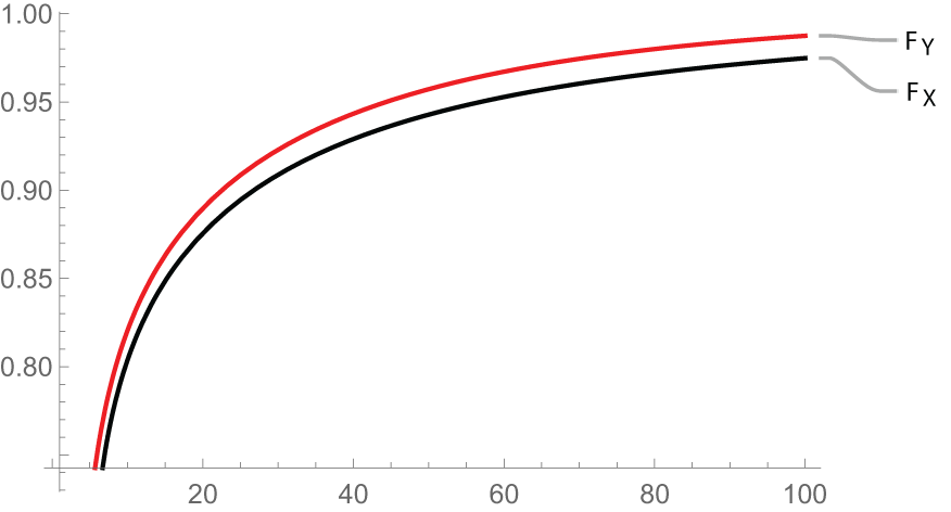

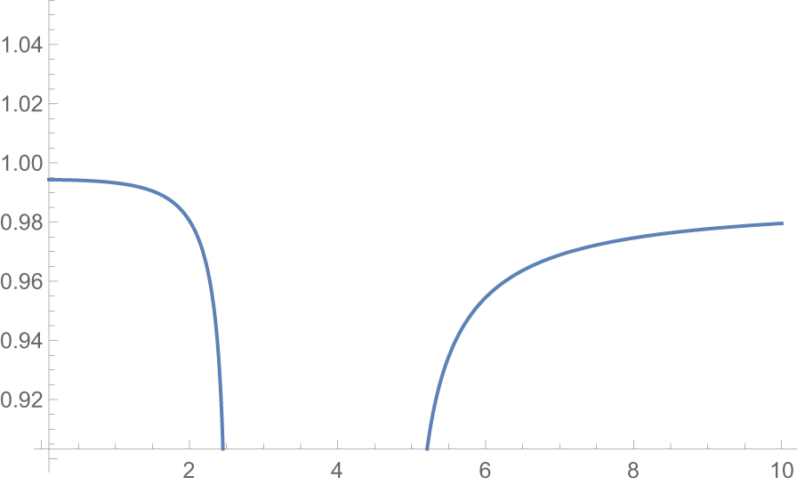

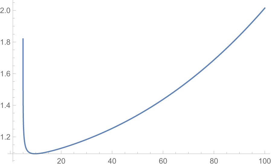

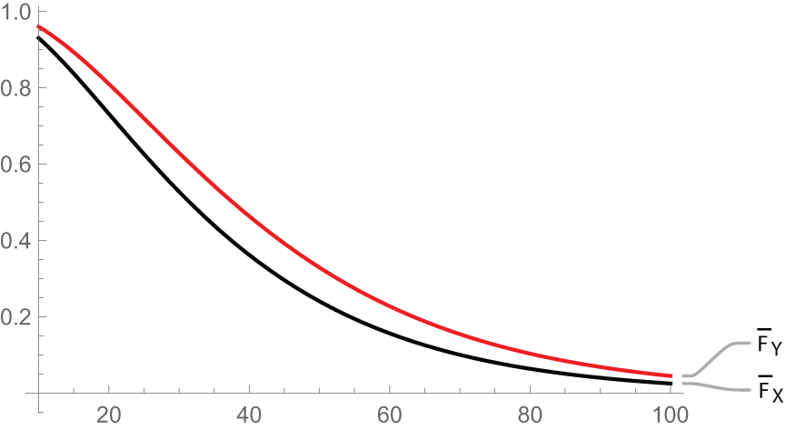

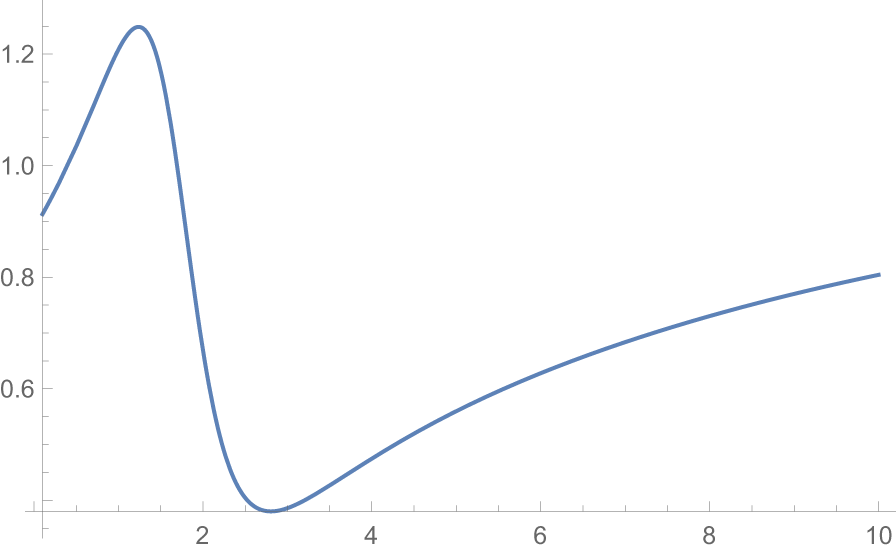

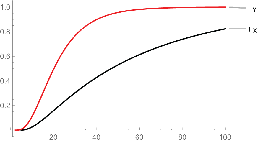


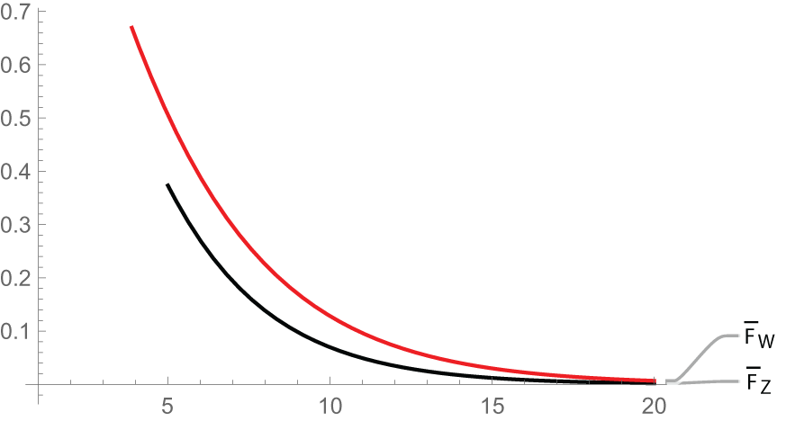


 Open access