


1. Introduction
Gravitation settling of small particles of complex shapes in a viscous fluid is observed in various systems, and it has been extensively studied in the literature. Examples are snowflakes in the air (Jayaweera & Mason Reference Jayaweera and Mason1966), natural floc sediments or mud in aquatic media (Strom & Keyvani Reference Strom and Keyvani2011; Spencer et al. Reference Spencer, Wheatland, Bushby, Carr, Droppo and Manning2021, Reference Spencer, Wheatland, Carr, Manning, Bushby, Gu, Botto and Lawrence2022; Gu et al. Reference Gu, Li, Spencer and Botto2026), marine snow in the oceans (Alldredge & Gotschalk Reference Alldredge and Gotschalk1988; Diercks & Asper Reference Diercks and Asper1997), swimming of micro-organisms denser than water (Rizvi et al. Reference Rizvi, Peyla, Farutin and Misbah2020; Larson et al. Reference Larson, Chajwa, Li and Prakash2024) or transport of microplastic fibres in water and air (Tatsii et al. Reference Tatsii, Bucci, Bhowmick, Guettler, Bakels, Bagheri and Stohl2024; Candelier et al. Reference Candelier, Gustavsson, Sharma, Sundberg, Pumir, Bagheri and Mehlig2025). Tatsii et al. (Reference Tatsii, Bucci, Bhowmick, Guettler, Bakels, Bagheri and Stohl2024) point out that the smaller the microplastic particle sedimentation velocity, the larger the distance it moves in the atmosphere, transported by wind. The distance can be as large as thousands of kilometres. On the other hand, the particle sedimentation velocity significantly depends on its shape. Anisotropic objects sedimenting under gravity undergo complex hydrodynamic interactions that have been analysed for numerous simplified model systems.
For larger particles, the inertia effects are important (Jayaweera & Mason Reference Jayaweera and Mason1965, Reference Jayaweera and Mason1966; Candelier & Mehlig Reference Candelier and Mehlig2016; Ravichandran & Wettlaufer Reference Ravichandran and Wettlaufer2023; Maches et al. Reference Maches, Houssais, Sauret and Meiburg2024; Tatsii et al. Reference Tatsii, Bucci, Bhowmick, Guettler, Bakels, Bagheri and Stohl2024; Candelier et al. Reference Candelier, Gustavsson, Sharma, Sundberg, Pumir, Bagheri and Mehlig2025). For micrometre-sized particles, the inertialess description is sufficient to reproduce the dynamics. In practice, depending on the context, it may mean the Reynolds number is smaller than of the order of one (Ravichandran & Wettlaufer Reference Ravichandran and Wettlaufer2023) or even smaller than 0.01 (Jayaweera & Mason Reference Jayaweera and Mason1965).
Sedimentation of single rigid particles of different complex shapes in a viscous fluid for a Reynolds number much smaller than unity has been studied for a very long time (see early papers by Brenner (Reference Brenner1963, Reference Brenner1964)). One of the basic tasks, investigated experimentally and numerically, e.g. by Lasso & Weidman (Reference Lasso and Weidman1986), Cichocki & Hinsen (Reference Cichocki and Hinsen1995) and Weber et al. (Reference Weber, Carlen, Dietler, Rawdon and Stasiak2013) for hollow cylinders, conglomerates of spheres and rigid knots, is to determine how much the particle’s settling velocity is smaller than the Stokes velocity of a sphere of equal mass and volume. In general, the settling velocity of elongated particles or disks depends on their orientation and is accompanied by a lateral drift (Lamb Reference Lamb1924, p. 605), (Taylor Reference Taylor1966). Moreover, depending on shape, a particle can rotate while settling.
For a particle settling under a given gravitational force in an incompressible viscous fluid, and generating a fluid flow satisfying the stationary Stokes equations, the particle angular velocity and the translational velocity of its centre-of-mass are determined, respectively, by the $3\times 3$
rotational–translational and translational–translational mobility matrices, evaluated with respect to the centre of mass, and applied to the gravitational force, as explained, e.g. by Happel & Brenner (Reference Happel and Brenner1965), Durlofsky, Brady & Bossis (Reference Durlofsky, Brady and Bossis1987), Felderhof (Reference Felderhof1988), Kim & Karrila (Reference Kim and Karrila1991) and Graham (Reference Graham2018). It is known that for chiral particles, there exists a rotational–translational coupling, which means that the rotational–translational mobility matrix evaluated with respect to the centre of mass is not zero. Coupled rotational and translational dynamics of chiral objects have been extensively studied, including rigid knots (Gonzalez, Graf & Maddocks Reference Gonzalez, Graf and Maddocks2004), chiral propeller-like shapes (Doi & Makino Reference Doi and Makino2005a
), asymmetric rigid fibres (Tozzi et al. Reference Tozzi, Scott, Vahey and Klingenberg2011; Vahey et al. Reference Vahey, Tozzi, Scott and Klingenberg2011), rigid helices (Palusa et al. Reference Palusa, De Graaf, Brown and Morozov2018) and helical rigid ribbons (Huseby et al. Reference Huseby, Gissinger, Candelier, Pujara, Verhille, Mehlig and Voth2025). However, the rotational–translational coupling can be non-zero also for particles with a non-chiral shape (see, e.g. Gonzalez et al. Reference Gonzalez, Graf and Maddocks2004; Doi & Makino Reference Doi and Makino2005b
). Examples are rigid non-chiral propellers considered by Kim & Karrila (Reference Kim and Karrila1991, p. 119), Makino & Doi (Reference Makino and Doi2003), Doi & Makino (Reference Doi and Makino2005b
) and Krapf, Witten & Keim (Reference Krapf, Witten and Keim2009), rigid trumbbells investigated numerically and theoretically by Ekiel-Jeżewska & Wajnryb (Reference Ekiel-Jeżewska and Wajnryb2009a
), bent rigid fibres (Candelier et al. Reference Candelier, Gustavsson, Sharma, Sundberg, Pumir, Bagheri and Mehlig2025) and bent rigid disks, studied experimentally, numerically and theoretically by Miara et al. (Reference Miara, Vaquero-Stainer, Pihler-Puzović, Heil and Juel2024) and Vaquero-Stainer et al. (Reference Vaquero-Stainer, Miara, Juel, Pihler-Puzović and Heil2024, Reference Vaquero-Stainer, Miara, Juel, Heil and Pihler-Puzović2026). In these papers, the non-chiral propellers, trumbbells and bent fibres and disks have two perpendicular symmetry planes.
$3\times 3$
rotational–translational and translational–translational mobility matrices, evaluated with respect to the centre of mass, and applied to the gravitational force, as explained, e.g. by Happel & Brenner (Reference Happel and Brenner1965), Durlofsky, Brady & Bossis (Reference Durlofsky, Brady and Bossis1987), Felderhof (Reference Felderhof1988), Kim & Karrila (Reference Kim and Karrila1991) and Graham (Reference Graham2018). It is known that for chiral particles, there exists a rotational–translational coupling, which means that the rotational–translational mobility matrix evaluated with respect to the centre of mass is not zero. Coupled rotational and translational dynamics of chiral objects have been extensively studied, including rigid knots (Gonzalez, Graf & Maddocks Reference Gonzalez, Graf and Maddocks2004), chiral propeller-like shapes (Doi & Makino Reference Doi and Makino2005a
), asymmetric rigid fibres (Tozzi et al. Reference Tozzi, Scott, Vahey and Klingenberg2011; Vahey et al. Reference Vahey, Tozzi, Scott and Klingenberg2011), rigid helices (Palusa et al. Reference Palusa, De Graaf, Brown and Morozov2018) and helical rigid ribbons (Huseby et al. Reference Huseby, Gissinger, Candelier, Pujara, Verhille, Mehlig and Voth2025). However, the rotational–translational coupling can be non-zero also for particles with a non-chiral shape (see, e.g. Gonzalez et al. Reference Gonzalez, Graf and Maddocks2004; Doi & Makino Reference Doi and Makino2005b
). Examples are rigid non-chiral propellers considered by Kim & Karrila (Reference Kim and Karrila1991, p. 119), Makino & Doi (Reference Makino and Doi2003), Doi & Makino (Reference Doi and Makino2005b
) and Krapf, Witten & Keim (Reference Krapf, Witten and Keim2009), rigid trumbbells investigated numerically and theoretically by Ekiel-Jeżewska & Wajnryb (Reference Ekiel-Jeżewska and Wajnryb2009a
), bent rigid fibres (Candelier et al. Reference Candelier, Gustavsson, Sharma, Sundberg, Pumir, Bagheri and Mehlig2025) and bent rigid disks, studied experimentally, numerically and theoretically by Miara et al. (Reference Miara, Vaquero-Stainer, Pihler-Puzović, Heil and Juel2024) and Vaquero-Stainer et al. (Reference Vaquero-Stainer, Miara, Juel, Pihler-Puzović and Heil2024, Reference Vaquero-Stainer, Miara, Juel, Heil and Pihler-Puzović2026). In these papers, the non-chiral propellers, trumbbells and bent fibres and disks have two perpendicular symmetry planes.
Sedimentation dynamics of bodies with two orthogonal planes of symmetry have been recently determined by Joshi & Govindarajan (Reference Joshi and Govindarajan2025). Namely, it was theoretically shown there that each shape belongs to one of three distinct families of solutions: settlers, which tend to a stationary stable orientation characterised by vertical terminal velocity; drifters, which tend to an inclined orientation and a lateral drift superimposed with a vertical translation; and flutterers, which undergo periodic oscillations while sedimenting.
In this paper, we focus on the dynamics of settlers. We provide experimental and numerical examples of the settler dynamics, and demonstrate that the typical times to approach the stationary stable orientation are short enough for potential applications (Spencer et al. Reference Spencer, Wheatland, Carr, Manning, Bushby, Gu, Botto and Lawrence2022; Tatsii et al. Reference Tatsii, Bucci, Bhowmick, Guettler, Bakels, Bagheri and Stohl2024). The choice of the experimental rigid shapes was motivated by an earlier work of Ekiel-Jeżewska & Wajnryb (Reference Ekiel-Jeżewska and Wajnryb
a2009) on sedimentation of a rigid trumbbell made of three identical spheres at the vertices of an isosceles (but not equilateral) triangle, and the middle sphere touching the other ones. It was shown there that the trumbbell rotates towards a stationary orientation with the middle sphere at the bottom. We chose various easily available shapes similar to a trumbbell: cone, arrowhead, crescent moon and open rings with four different sizes of the opening. Indeed, it turned out that they are all settlers. However, it was not evident which of the two stationary symmetric orientations would be stable: the arrowhead, crescent moon and open rings reoriented as the trumbbell: ‘the wider side up’, but the cone’s stable position is ‘the wider side down’. One might intuitively guess that for the cone, ‘the wider side down’ is the stable orientation, because this side is heavier (as in the case of asymmetric dumbbells studied by Candelier & Mehlig (Reference Candelier and Mehlig2016) and Nissanka, Ma & Burton (Reference Nissanka, Ma and Burton2023)), but this argument does not hold for the trumbbell studied by Ekiel-Jeżewska & Wajnryb (Reference Ekiel-Jeżewska and Wajnryb2009a
) and for the other shapes used in our experiments. Moreover, Jayaweera & Mason (Reference Jayaweera and Mason1965) showed that for larger Reynolds numbers, Re $\geqslant 0.5$
, the cones with a small apex angle
$\geqslant 0.5$
, the cones with a small apex angle $\lt \pi /4$
reorient the apex up, and with a large apex angle
$\lt \pi /4$
reorient the apex up, and with a large apex angle $\gt \pi /4$
– the apex down, and no corresponding results for
$\gt \pi /4$
– the apex down, and no corresponding results for $Re\ll 1$
are available.
$Re\ll 1$
are available.
As determined theoretically by Joshi & Govindarajan (Reference Joshi and Govindarajan2025), for ${Re} \ll 1$
, the dynamics of a rigid particle with two orthogonal symmetry planes are qualitatively different for different signs of the product of the rotational–translational mobility coefficients,
${Re} \ll 1$
, the dynamics of a rigid particle with two orthogonal symmetry planes are qualitatively different for different signs of the product of the rotational–translational mobility coefficients, $\mu _{42}$
and
$\mu _{42}$
and $ \mu _{51}$
, evaluated with respect to the particle centre of mass in the symmetric reference frame
$ \mu _{51}$
, evaluated with respect to the particle centre of mass in the symmetric reference frame $xyz$
shown in figure 1(c). For a given particle’s shape, we show how to determine
$xyz$
shown in figure 1(c). For a given particle’s shape, we show how to determine $\mu _{42}$
and
$\mu _{42}$
and $ \mu _{51}$
from the experiments, choosing two different special initial orientations. We also estimate
$ \mu _{51}$
from the experiments, choosing two different special initial orientations. We also estimate $\mu _{42}$
and
$\mu _{42}$
and $\mu _{51}$
numerically, based on the Stokes equations. We propose a method for accomplishing this, using the bead model. Then, we apply it to the particles studied experimentally in this work (the settlers, for which
$\mu _{51}$
numerically, based on the Stokes equations. We propose a method for accomplishing this, using the bead model. Then, we apply it to the particles studied experimentally in this work (the settlers, for which $\mu _{42} \, \mu _{51} \lt 0$
). Values of the rotational–translational mobility coefficients evaluated numerically are next shown to estimate reasonably well the corresponding values extracted from the experiments, justifying that they are settlers, and allowing to predict the time scales of their reorientation. The experimental and theoretical methods to determine
$\mu _{42} \, \mu _{51} \lt 0$
). Values of the rotational–translational mobility coefficients evaluated numerically are next shown to estimate reasonably well the corresponding values extracted from the experiments, justifying that they are settlers, and allowing to predict the time scales of their reorientation. The experimental and theoretical methods to determine $\mu _{42}$
and
$\mu _{42}$
and $ \mu _{51}$
, presented in this paper, can also be used for the flutterers (for which
$ \mu _{51}$
, presented in this paper, can also be used for the flutterers (for which $\mu _{42} \, \mu _{51} \gt 0$
) and drifters (with
$\mu _{42} \, \mu _{51} \gt 0$
) and drifters (with $\mu _{42} \, \mu _{51} = 0$
).
$\mu _{42} \, \mu _{51} = 0$
).
The structure of the paper is the following. In § 2, we provide the theoretical background and explain the characteristic feature of the rotational–translational mobility matrix for the settlers. In § 3, the experimental set-up, the particles and the methods are described. Section 4 presents the experimental results: initial orientations and statistics of the experimental trials; typical examples of the translation and rotation of particles, shown by the time sequence of snapshots; the time-dependent vertical velocity; the time-dependent inclination angle, as well as the average values of the mobility coefficients. In § 5, the experimental shapes are approximated as conglomerates of identical spherical beads, and their mobility coefficients are determined numerically. Section 6 contains a comparison of the theoretical and experimental results, and § 7 is devoted to a parametric numerical study of the aperture-controlled rings. Finally, § 8 presents conclusions.
2. Theoretical background
We consider a rigid particle moving in a viscous fluid under the reduced weight $\boldsymbol{F}$
, equal to gravity minus buoyancy. The Reynolds number Re
$\boldsymbol{F}$
, equal to gravity minus buoyancy. The Reynolds number Re $\ll$
1, and the fluid velocity
$\ll$
1, and the fluid velocity $\boldsymbol{v}(\boldsymbol{r})$
and pressure
$\boldsymbol{v}(\boldsymbol{r})$
and pressure $p(\boldsymbol{r})$
are described by the stationary Stokes equations,
$p(\boldsymbol{r})$
are described by the stationary Stokes equations,
 \begin{align} \eta {\nabla }^2 \boldsymbol{v} - \boldsymbol{\nabla } p=\boldsymbol{0},\quad \boldsymbol{\nabla }\boldsymbol{\cdot }\boldsymbol{v}=0. \end{align}
The motion of the particle is derived from (2.1), assuming the no slip boundary conditions for the fluid at the particle surface (Kim & Karrila Reference Kim and Karrila1991; Graham Reference Graham2018). The particle translational and angular velocities, $\boldsymbol{U}$
and
$\boldsymbol{U}$
and $\boldsymbol{\varOmega }$
, are linear functions of the Cartesian components of the reduced weight
$\boldsymbol{\varOmega }$
, are linear functions of the Cartesian components of the reduced weight $\boldsymbol{F}$
acting on the particle. In the laboratory frame of reference
$\boldsymbol{F}$
acting on the particle. In the laboratory frame of reference $XYZ$
, the reduced weight
$XYZ$
, the reduced weight $\boldsymbol{F}$
is antiparallel to the
$\boldsymbol{F}$
is antiparallel to the $Z$
-axis,
$Z$
-axis, $\boldsymbol{F}=-F\boldsymbol{\hat {Z}}$
. We calculate
$\boldsymbol{F}=-F\boldsymbol{\hat {Z}}$
. We calculate $\boldsymbol{U}$
with respect to the centre of mass. The benefit is that the torque vanishes with respect to the centre of mass, and therefore,
$\boldsymbol{U}$
with respect to the centre of mass. The benefit is that the torque vanishes with respect to the centre of mass, and therefore,
 \begin{eqnarray} &&\left (\begin{array}{@{}l@{}}\boldsymbol{U}\\ \boldsymbol{\varOmega }\end{array}\right ) = \left (\begin{array}{ll}\boldsymbol{\mu }^{\textit{tt}} \,\boldsymbol{\mu }^{tr}\\ \boldsymbol{\mu }^{\textit{rt}} \, \boldsymbol{\mu }^{\textit{rr}}\end{array}\right ) \boldsymbol{\cdot } \left (\begin{array}{@{}l@{}} \boldsymbol{F}\\ \boldsymbol{0}\end{array}\right )\!, \end{eqnarray}
or alternatively,
 \begin{eqnarray} &&\boldsymbol{U}= \boldsymbol{\mu }^{\textit{tt}} \boldsymbol{\cdot }\boldsymbol{F},\hspace {1cm} \boldsymbol{\varOmega } = \boldsymbol{\mu }^{\textit{rt}} \boldsymbol{\cdot }\boldsymbol{F}. \end{eqnarray}
The translational-translational mobility $\boldsymbol{\mu}^{tt}$
and the rotational-translational mobility
$\boldsymbol{\mu}^{tt}$
and the rotational-translational mobility $\boldsymbol{\mu}^{rt}$
are
$\boldsymbol{\mu}^{rt}$
are $3 \times 3$
Cartesian matrices that depend on the particle orientation.
$3 \times 3$
Cartesian matrices that depend on the particle orientation.
In this paper, as Joshi & Govindarajan (Reference Joshi and Govindarajan2025) and Ekiel-Jeżewska & Wajnryb (Reference Ekiel-Jeżewska and Wajnryb2009a
) in their theoretical studies, we focus on the particles having two perpendicular symmetry planes (but not symmetric with respect to reflection in the third perpendicular plane). We choose the frame of reference with the coordinates $x$
and
$x$
and $y$
perpendicular to the symmetry planes, and with the
$y$
perpendicular to the symmetry planes, and with the $x$
-coordinate along
$x$
-coordinate along $L$
– the larger from
$L$
– the larger from $x$
and
$x$
and $y$
sizes of the particle. (Most of our particles are rather flat – their size along
$y$
sizes of the particle. (Most of our particles are rather flat – their size along $y$
is smaller than along
$y$
is smaller than along $x$
; for the cone, exceptionally,
$x$
; for the cone, exceptionally, $x$
and
$x$
and $y$
sizes are the same.) In this special frame of reference, the dimensionless mobility matrices have the form
$y$
sizes are the same.) In this special frame of reference, the dimensionless mobility matrices have the form
 \begin{eqnarray} &&\pi \eta L \boldsymbol{\mu }^{\textit{tt}}=\left (\begin{matrix}\mu _{11} &0 &0\\ 0 & \mu _{22} &0\\ 0& 0 & \mu _{33} \end{matrix} \right ),\quad \pi \eta L^2 \boldsymbol{\mu }^{\textit{rt}} = \left (\begin{matrix} 0 & \mu _{42} & 0\\ \mu _{51} & 0 & 0\\ 0& 0 &0\end{matrix} \right ). \end{eqnarray}
In the following, we will use $L$
as the length unit, and the dimensionless time
$L$
as the length unit, and the dimensionless time $t$
defined as
$t$
defined as
 \begin{eqnarray} t=\frac {F}{\pi \eta L^2}\tilde {t}, \end{eqnarray}
with $F=|\boldsymbol{F}|$
and
$F=|\boldsymbol{F}|$
and $\tilde {t}$
denoting the dimensional time.
$\tilde {t}$
denoting the dimensional time.
Two special motions of a particle with $x\rightarrow -x$
and
$x\rightarrow -x$
and $y\rightarrow -y$
symmetries are illustrated: (a) case A, rotation of the particle around
$y\rightarrow -y$
symmetries are illustrated: (a) case A, rotation of the particle around $y=Y$
; (b) case B, rotation of the particle around
$y=Y$
; (b) case B, rotation of the particle around $x=X$
. Here
$x=X$
. Here $xyz$
is the coordinate system moving with the particle, shown in (c),
$xyz$
is the coordinate system moving with the particle, shown in (c), $XYZ$
is the laboratory frame of reference and
$XYZ$
is the laboratory frame of reference and $\theta$
is the angle between the
$\theta$
is the angle between the $z$
and
$z$
and $Z$
axes.
$Z$
axes.

We consider such particles that rotate and approach a stationary orientation, regardless of the initial conditions. This family of shapes has been called ‘settlers’ in the theoretical study by Joshi & Govindarajan (Reference Joshi and Govindarajan2025). For the settlers, the rotational–translational coefficients $\mu _{42}$
and
$\mu _{42}$
and $\mu _{51}$
are different from zero and have the opposite signs,
$\mu _{51}$
are different from zero and have the opposite signs,
 \begin{eqnarray} && \mu _{42} \,\mu _{51} \lt 0. \end{eqnarray}
The question is how to determine $\mu _{42}$
and
$\mu _{42}$
and $\mu _{51}$
from experiments. There are two special motions for which the dynamics are very simple, as shown by Ekiel-Jeżewska & Wajnryb (Reference Ekiel-Jeżewska and Wajnryb2009a
). These special cases A and B are illustrated in figure 1, using the laboratory frame of reference
$\mu _{51}$
from experiments. There are two special motions for which the dynamics are very simple, as shown by Ekiel-Jeżewska & Wajnryb (Reference Ekiel-Jeżewska and Wajnryb2009a
). These special cases A and B are illustrated in figure 1, using the laboratory frame of reference $XYZ$
and the frame of reference
$XYZ$
and the frame of reference $xyz$
moving with the particle.
$xyz$
moving with the particle.
For case A (shown in figure 1
a), if we choose the initial conditions in such a way that the axes $y$
and
$y$
and $Y$
are parallel to each other, then, owing to symmetry,
$Y$
are parallel to each other, then, owing to symmetry, $y$
and
$y$
and $Y$
stay parallel all the time, and the motion of the centre of mass takes place in the plane
$Y$
stay parallel all the time, and the motion of the centre of mass takes place in the plane $XZ$
. The particle orientation is specified by the angle
$XZ$
. The particle orientation is specified by the angle $\theta (t)$
between the axes
$\theta (t)$
between the axes $Z$
and
$Z$
and $z$
which evolves with time
$z$
which evolves with time $t$
as
$t$
as
 \begin{eqnarray} && \frac {\mathrm{d}\theta }{\mathrm{d}t}= \mu _{51} \sin \theta . \end{eqnarray}
For case B (shown in figure 1
b), if we choose the initial conditions in such a way the axes $x$
and
$x$
and $X$
are parallel to each other, then, owing to symmetry,
$X$
are parallel to each other, then, owing to symmetry, $x$
and
$x$
and $X$
stay parallel all the time, and the motion of the centre of mass takes place in the plane
$X$
stay parallel all the time, and the motion of the centre of mass takes place in the plane $YZ$
. The particle orientation is specified by the angle
$YZ$
. The particle orientation is specified by the angle $\theta (t)$
between the axis
$\theta (t)$
between the axis $Z$
and
$Z$
and $z$
which evolves with time
$z$
which evolves with time $t$
as
$t$
as
 \begin{eqnarray} && \frac {\mathrm{d}\theta }{\mathrm{d}t}= -\mu _{42} \sin \theta . \end{eqnarray}
Here, (2.7) and (2.8) are identical to the equation (14) introduced by Ekiel-Jeżewska & Wajnryb (Reference Ekiel-Jeżewska and Wajnryb2009a ) and solved there as their equation (15). Therefore, the solutions of (2.7) and (2.8) for cases A and B read
 \begin{align} \tan (\theta /2) & = A \exp (\mu _{51} t), \\[-10pt] \nonumber \end{align}
 \begin{align} \tan (\theta /2) & = A \exp (-\mu _{42} t). \\[10pt] \nonumber \end{align}
The general expressions for the settler’s non-planar motion are given by Ekiel-Jeżewska & Wajnryb (Reference Ekiel-Jeżewska and Wajnryb2009a
) in their equations (10)–(12) and also by Joshi & Govindarajan (Reference Joshi and Govindarajan2025). To simplify the analysis, in the experiments we aimed towards providing the initial orientation of the particle as in case A or case B, measuring the angle $\theta$
as a function of time, and then comparing with the corresponding solution from (2.9) or (2.10), as it will be described in § 4. In the experiments, we will analyse directly the dimensional quantities, and in particular, the time coefficients defined as
$\theta$
as a function of time, and then comparing with the corresponding solution from (2.9) or (2.10), as it will be described in § 4. In the experiments, we will analyse directly the dimensional quantities, and in particular, the time coefficients defined as
 \begin{eqnarray} \tilde {\tau }_{51} \equiv \frac {\pi \eta L^2}{F} \frac {1}{\mu _{51}},\,\, \mbox{ and }\,\,\,\, \tilde {\tau }_{42} \equiv \frac {\pi \eta L^2}{F} \frac {1}{\mu _{42}}, \end{eqnarray}
from the requirements that $\mu _{51}t=\tilde {t}/\tilde {\tau }_{51}$
and
$\mu _{51}t=\tilde {t}/\tilde {\tau }_{51}$
and $\mu _{42}t=\tilde {t}/\tilde {\tau }_{42}$
.
$\mu _{42}t=\tilde {t}/\tilde {\tau }_{42}$
.
In the experiments, we will show that particles reorient and reach the stationary configuration (see § 4). By measuring the final vertical stationary centre-of-mass velocity $U_{\!f}$
, and the reduced weight
$U_{\!f}$
, and the reduced weight $F$
, we will determine the dimensionless translational–translational mobility coefficient relevant for the particle translation in the stationary state,
$F$
, we will determine the dimensionless translational–translational mobility coefficient relevant for the particle translation in the stationary state,
 \begin{eqnarray} && \mu _{33} = \pi \eta L \frac {U_{\!f}}{F}. \end{eqnarray}
Each of the particle shapes used in our experiments is later approximated as a collection of touching beads, and the mobility coefficients in (2.4) are evaluated by the multipole method corrected for lubrication, outlined by Cichocki, Ekiel-Jeżewska & Wajnryb (Reference Cichocki, Ekiel-Jeżewska and Wajnryb1999) and Ekiel-Jeżewska & Wajnryb (Reference Ekiel-Jeżewska and Wajnryb2009b ) (see § 5 for the results).
3. Experimental system, materials and methods
3.1. Experimental set-up
The experimental set-up is almost the same as the one used by Shashank, Melikhov & Ekiel-Jeżewska (Reference Shashank, Melikhov and Ekiel-Jeżewska2023), but without a mirror. The experiments are conducted in the glass tank of inner dimension 200 mm $\times$
200 mm
$\times$
200 mm $\times$
500 mm (width, depth and height, respectively). We utilise the highly viscous silicone oil (manufactured by Silikony Polskie) with the kinematic viscosity
$\times$
500 mm (width, depth and height, respectively). We utilise the highly viscous silicone oil (manufactured by Silikony Polskie) with the kinematic viscosity $\nu = 5 \boldsymbol{\times }10^{-3} \,\text{m}^2 \;\text{s}^{-1}$
and density
$\nu = 5 \boldsymbol{\times }10^{-3} \,\text{m}^2 \;\text{s}^{-1}$
and density $\rho = 970 \,\text{kg m}^{-3}$
at 25
$\rho = 970 \,\text{kg m}^{-3}$
at 25 $^\circ$
C. Solid objects (in the following called particles) with two orthogonal planes of symmetry are dropped in this tank to study if they reorient and approach a stationary configuration. Particle motion is recorded using two cameras placed perpendicularly to the front and side of the tank, with the line of sight directed to the centre of the wall. Both cameras point at the glass tank directly, and both lamps are kept parallel to the walls of the tank with the diffusers to get equal illumination throughout the tank area, as shown in figure 2. The arrangement of the light source, tank and cameras ensures that the opaque sedimenting particles are clearly visible on a bright background.
$^\circ$
C. Solid objects (in the following called particles) with two orthogonal planes of symmetry are dropped in this tank to study if they reorient and approach a stationary configuration. Particle motion is recorded using two cameras placed perpendicularly to the front and side of the tank, with the line of sight directed to the centre of the wall. Both cameras point at the glass tank directly, and both lamps are kept parallel to the walls of the tank with the diffusers to get equal illumination throughout the tank area, as shown in figure 2. The arrangement of the light source, tank and cameras ensures that the opaque sedimenting particles are clearly visible on a bright background.
We use two identical full-frame DSLR cameras (Canon 5D Mark IV) with a resolution of 30 megapixels, equipped with 100 mm prime lenses. The cameras are connected to a multiple-camera operation trigger box (manufactured by Esper Ltd., U.K.). The cameras are triggered simultaneously using the Esper trigger box operating software, controlled by the computer set-up. The time delay of the trigger box for triggering both cameras simultaneously is 20 ms. The images are captured at the rate of 1 frame per second (f.p.s.). Both cameras are set with the highest available $f$
-number,
$f$
-number, $f=32$
(corresponding to the smallest aperture) and with an exposure time of 1/25 s.
$f=32$
(corresponding to the smallest aperture) and with an exposure time of 1/25 s.
The distance travelled by the object in the given exposure time is in the range of 1–7 pixels. The motion of the object during the exposure time can be seen as blurring of the image. The influence of the blurring on extracting values of the angle $\theta$
is analysed in Appendix B, with the conclusion that the effect of the motion blur can be safely neglected in the present study. The ISO of both cameras is kept at 160 to achieve sufficient brightness with a moderate noise level.
$\theta$
is analysed in Appendix B, with the conclusion that the effect of the motion blur can be safely neglected in the present study. The ISO of both cameras is kept at 160 to achieve sufficient brightness with a moderate noise level.
Schematic representation of the experimental set-up.

Both cameras are arranged in portrait orientation, positioned equidistant from the front and side faces of the tank at approximately 820 mm. This distance has been selected to ensure the complete field of view captured by each camera, covering slightly more than 300 mm vertically and 200 mm horizontally across the height and width of the tank, respectively. Both cameras are aligned at the tank’s midheight. This set-up avoids recording the particle motion closer than $\sim$
100 mm from the top or bottom of the fluid to avoid recording a particle’s strong hydrodynamic interaction with the free surface and the bottom wall. Note that all the settings in both cameras are identical as described in the above section.
$\sim$
100 mm from the top or bottom of the fluid to avoid recording a particle’s strong hydrodynamic interaction with the free surface and the bottom wall. Note that all the settings in both cameras are identical as described in the above section.
3.2. Rigid particles
The study involves rigid objects (sourced from Koniarscy S. C., Poland) of different shapes with two perpendicular symmetry planes, non-symmetric with respect to reflections in the third perpendicular plane: crescent moons and cones made of glass, arrowheads fabricated from haematite (non-magnetic) and open rings made of steel. We opened the rings manually, adjusting the size of the gap between the ends.
Figure 3 presents the real images of the objects used in this study in the $xyz$
reference frame moving with the particle, with the
$xyz$
reference frame moving with the particle, with the $z$
axis at the intersection of the symmetry planes
$z$
axis at the intersection of the symmetry planes $xz$
and
$xz$
and $yz$
. All dimensions shown in figure 3 were measured using a high-precision digital vernier calliper with an accuracy of 0.01 mm per measurement. Each measurement was performed on at least five objects and repeated two to three times to take into account that the dimensions of individual objects may vary, and to minimise measurement errors. The dimensions of the objects and their standard deviations are as follows.
$yz$
. All dimensions shown in figure 3 were measured using a high-precision digital vernier calliper with an accuracy of 0.01 mm per measurement. Each measurement was performed on at least five objects and repeated two to three times to take into account that the dimensions of individual objects may vary, and to minimise measurement errors. The dimensions of the objects and their standard deviations are as follows.
-
(i) Cone-shaped objects. The diameter is $L= 4.39 \pm 0.02$
mm, and the height is
$H=10.45 \pm 0.05$
mm. A cylindrical hole with a diameter of
$0.96\pm 0.05$
mm passes through the cone, parallel to the base and intersecting the central axis at a height of
$1.70 \pm 0.01$
mm from the base.
$L= 4.39 \pm 0.02$
mm, and the height is
$H=10.45 \pm 0.05$
mm. A cylindrical hole with a diameter of
$0.96\pm 0.05$
mm passes through the cone, parallel to the base and intersecting the central axis at a height of
$1.70 \pm 0.01$
mm from the base. -
(ii) Crescent moon-shaped objects. The length is
$L=10.18 \pm 0.02$
mm, the total height is
$H=4.46 \pm 0.09$
mm, the middle height is
$S=3.91 \pm 0.14$
mm and the width varies, with the middle width equal to
$W_M=2.13 \pm 0.02$
mm. Two holes with a diameter of
$0.85\pm 0.02$
mm pass through the thickness of the crescent moon-shaped object. They are positioned symmetrically,
$1.47 \pm 0.06$
mm above the base, with a centre-to-centre separation of
$2.99 \pm 0.04$
mm. -
(iii) Arrowhead-shaped objects. The length is
$L=6.28 \pm 0.08$
mm, the total height is
$H=4.93 \pm 0.08$
mm, the middle height is
$S=3.81 \pm 0.02$
mm and the width is
$W=2.33 \pm 0.10$
mm. A hole, coaxial with
$z$
, of a diameter of
$1.06\pm 0.02$
mm, extends through the arrowhead, emerging at the apex. -
(iv) Open rings. We measured length
$L$
and height
$H$
of the rings as
$L=5.45 \pm 0.01$
mm,
$L=5.92 \pm 0.04$
mm,
$L=6.48 \pm 0.08$
mm,
$L=6.81 \pm 0.02$
mm and
$H=4.95 \pm 0.01$
mm,
$H=4.90 \pm 0.02$
mm,
$H=4.88 \pm 0.03$
mm,
$H=4.86 \pm 0.02$
mm, respectively, for the rings with the openings of
$1.02 \pm 0.05$
mm,
$2.02 \pm 0.06$
mm,
$3.02 \pm 0.05$
mm and
$4.02 \pm 0.05$
mm, respectively. The width of all the rings remains constant at
$W=0.596 \pm 0.005$
mm.


The objects used in the experimental studies, shown from different perspectives, with their dimensions indicated in millimetres. The scale bar (white line) represents 5 mm.

The physical properties of the objects: mass, volume and the reduced weight $F$
equal to gravity minus buoyancy are presented in table 1. The masses of the objects were obtained using a high-performance analytical balance with a measuring accuracy of 0.1 mg per measurement. However, the masses of individual objects of the same type varied. Therefore, the mass measurements were conducted on at least 10 objects of the same type, and the average values and their standard deviations were listed in table 1. The volume of the cones, arrowheads, and crescent moons was measured experimentally using the water displacement method, a well-established technique for irregularly shaped solids. For the arrowhead and crescent moon, we used 50 particles and assumed the displaced water volume to be equal to the total volume of all the particles. Due to the unavailability of materials from the same batch, we used only 12 cone particles for volume measurement. In this way, we determined the average volume of a single object. However, for much smaller rings, the volume was calculated more precisely by measuring the dimensions of several closed rings, averaging them and using the geometric formula of a torus volume. The average mass and volume were then used to evaluate the average reduced weight
$F$
equal to gravity minus buoyancy are presented in table 1. The masses of the objects were obtained using a high-performance analytical balance with a measuring accuracy of 0.1 mg per measurement. However, the masses of individual objects of the same type varied. Therefore, the mass measurements were conducted on at least 10 objects of the same type, and the average values and their standard deviations were listed in table 1. The volume of the cones, arrowheads, and crescent moons was measured experimentally using the water displacement method, a well-established technique for irregularly shaped solids. For the arrowhead and crescent moon, we used 50 particles and assumed the displaced water volume to be equal to the total volume of all the particles. Due to the unavailability of materials from the same batch, we used only 12 cone particles for volume measurement. In this way, we determined the average volume of a single object. However, for much smaller rings, the volume was calculated more precisely by measuring the dimensions of several closed rings, averaging them and using the geometric formula of a torus volume. The average mass and volume were then used to evaluate the average reduced weight $F$
(gravity minus buoyancy). The averages and their uncertainties are listed in table 1. Finally, note that we conducted experiments with different objects of the same type, with each object being used only once, and we approximated their mass, volume and reduced weight using the average values.
$F$
(gravity minus buoyancy). The averages and their uncertainties are listed in table 1. Finally, note that we conducted experiments with different objects of the same type, with each object being used only once, and we approximated their mass, volume and reduced weight using the average values.
Physical properties of the various objects used during the experimental study.

3.3. Methodology
The experiments were performed by manually dropping the object from the top of the tank, approximately at the centre of the fluid surface. The cameras were triggered when the object inside the tank was about to reach the visible zone of the cameras, and stopped when the object came out of the camera’s image.
Before performing each series of the experimental trials, we put the ruler at the central vertical line of the outside container walls facing both cameras, and we adjusted the camera positions to reach the same height $h$
of the recorded images from both cameras. The motion of the objects took place close to the central vertical line of the container. The real height
$h$
of the recorded images from both cameras. The motion of the objects took place close to the central vertical line of the container. The real height $h'$
of the image at this line was larger than
$h'$
of the image at this line was larger than $h$
owing to a finite camera viewing angle, decreased by the refraction of the light (the refractive index of the silicon oil is 1.4). For our set-up, we measured the real image height
$h$
owing to a finite camera viewing angle, decreased by the refraction of the light (the refractive index of the silicon oil is 1.4). For our set-up, we measured the real image height $h'$
by putting the ruler inside the tank at its central line, and measuring the apparent image height
$h'$
by putting the ruler inside the tank at its central line, and measuring the apparent image height $h$
by putting the other ruler at the central vertical line of the outside front wall of the container. In this way, we determined the correction factor
$h$
by putting the other ruler at the central vertical line of the outside front wall of the container. In this way, we determined the correction factor $h'/h=1.077$
, and we used this factor to recalculate the time-dependent particle positions from pixels to millimetres. Approximately one pixel was around 0.052 mm, but this calibration factor was determined specifically for each series of the experiments.
$h'/h=1.077$
, and we used this factor to recalculate the time-dependent particle positions from pixels to millimetres. Approximately one pixel was around 0.052 mm, but this calibration factor was determined specifically for each series of the experiments.
We used both prewetted and non-prewetted particles. In certain experimental trials for the non-prewetted cones, arrowheads and crescent moons, we observed a single small bubble, moved out from a hole in the object, temporarily attached to the object and next separated from it, sometimes splitting into smaller ones. However, we carefully analysed that a small bubble attached to an object does not significantly modify its mobility coefficients (e.g. particle settling velocity $U_{\kern-1pt f}$
is not decreased by more than 2 %). The only significant difference is that for non-prewetted crescent moons, bubbles changed the particle orientation before it entered the camera’s field of view.
$U_{\kern-1pt f}$
is not decreased by more than 2 %). The only significant difference is that for non-prewetted crescent moons, bubbles changed the particle orientation before it entered the camera’s field of view.
The motion and reorientation of objects were recorded in the time sequence of the camera images. Further, all the images were transferred into MATLAB, and image analysis was performed to identify the objects there. Image processing steps involved the binarisation of the RGB images, background subtraction and thresholding to obtain clearer shapes of the objects. Additionally, noise removal techniques were employed to avoid spurious object detection in the cameras caused by shadows and reflections of the objects under high illumination.
4. Experimental results
4.1. Initial orientations and the number of experimental trials
In the experiments, we have controlled the initial orientations of the particles at the fluid surface. As it has already been stated before, the cameras started to record the particles after they settled around 10 cm from the fluid free surface, and changed their orientation from the initial one.
In the preliminary trials, it was observed that all the shapes approached a stationary orientation for different initial configurations. Then, we conducted experimental trials for three distinct families of initial orientations at the fluid free surface:
-
(i) stationary;
-
(ii) inverted;
-
(iii) inclined.
The ‘stationary’ initial orientation, with $x=X$
,
$x=X$
, $y=Y$
and
$y=Y$
and $z=Z$
, was chosen to confirm that this orientation indeed remains stationary. We performed 27 such experiments, and indeed, in all of them, the particle orientation did not change with time.
$z=Z$
, was chosen to confirm that this orientation indeed remains stationary. We performed 27 such experiments, and indeed, in all of them, the particle orientation did not change with time.
The ‘inverted’ initial orientation, with $x=-X$
,
$x=-X$
, $y=Y$
and
$y=Y$
and $z=-Z$
, was chosen aiming to observe the particle rotation around
$z=-Z$
, was chosen aiming to observe the particle rotation around $y=Y$
axis, perpendicular to the plane of view of camera 1 (case A shown in figure 1
a), and its centre of mass moving in the
$y=Y$
axis, perpendicular to the plane of view of camera 1 (case A shown in figure 1
a), and its centre of mass moving in the $xz$
plane, equal to the
$xz$
plane, equal to the $XZ$
plane. Such a motion allows to measure the rotational–translational mobility coefficient
$XZ$
plane. Such a motion allows to measure the rotational–translational mobility coefficient $\mu _{51}$
from the theoretical relation (2.9).
$\mu _{51}$
from the theoretical relation (2.9).
The ‘inclined’ initial orientation, with $x=X$
, and the angle
$x=X$
, and the angle $\theta$
between
$\theta$
between $z$
and
$z$
and $Z$
axes larger than
$Z$
axes larger than $\pi /2$
and close to
$\pi /2$
and close to $\pi$
, was chosen aiming to observe the particle rotation around
$\pi$
, was chosen aiming to observe the particle rotation around $x=X$
axis, perpendicular to the plane of view of camera 2 (case B shown in figure 1
b), and therefore to measure the rotational–translational mobility coefficient
$x=X$
axis, perpendicular to the plane of view of camera 2 (case B shown in figure 1
b), and therefore to measure the rotational–translational mobility coefficient $\mu _{42}$
from the theoretical relation (2.10). In this case, the centre of mass moves in the
$\mu _{42}$
from the theoretical relation (2.10). In this case, the centre of mass moves in the $yz$
plane, equal to the
$yz$
plane, equal to the $YZ$
plane.
$YZ$
plane.
In table 2 we list the numbers of the experimental trials performed with each type of particle, for all the initial orientations: stationary, inverted and inclined. In 155 experimental trials, we observed the particle reorienting to a stable, stationary orientation (110 trials for the inverted initial orientation and 45 trials for the inclined initial orientation). In addition, 27 trials showed particles of various types remaining at a stationary, stable orientation throughout the entire experiment. Therefore, in this work, we performed 182 experimental trials overall.
The number of experimental trials performed for the indicated initial orientations of the objects, along with the number of trials selected for quantitative analysis of the reorientation. Names of the objects: C, cone; A, arrowhead; M, crescent moon; R $i$
, ring with the opening width equal to
$i$
, ring with the opening width equal to $i = 1, 2, 3, 4$
mm. For the crescent moon, the numbers without and with an asterisk refer to the trials with non-prewetted and prewetted particles, used to compute
$i = 1, 2, 3, 4$
mm. For the crescent moon, the numbers without and with an asterisk refer to the trials with non-prewetted and prewetted particles, used to compute $\mu _{42}$
and
$\mu _{42}$
and $\mu _{51}$
, respectively.
$\mu _{51}$
, respectively.

All the reported experimental trials are presented in the repository, Shekhar et al. (Reference Shekhar, Mirajkar, Zdybel, Melikhov and Ekiel-Jeżewska2025). In some of them, the initial conditions trigger a complex motion. Examples are shown in Appendix A. It would be difficult to extract values of the rotational–translational mobility coefficients from these trials. Fortunately, in agreement with our intentions, the chosen initial conditions often lead to one of two special motions, labelled as case A and case B, and illustrated in figure 1. For both special cases, the solution of the dynamics is analytical and very simple, as shown in (2.9) and (2.10). Therefore, from all the trials, we selected cases A and B mentioned above and used them for an easy determination of $\mu _{51}$
and
$\mu _{51}$
and $\mu _{42}$
, respectively.
$\mu _{42}$
, respectively.
4.2. Results for the stationary and inverted initial orientations
We recorded the reorientation of sedimenting single cones, crescent moons, arrowheads and open rings in 110 experimental trials for the inverted initial orientations. We used both prewetted and non-prewetted particles. In all the trials performed for the same type of particle, it was observed that the particle always approached the same stationary orientation and remained there for a long time. In some cases, the particle motion was more complex than it had been predicted, involving also other components of the angular velocity, and a few trials could not be analysed quantitatively because the reorientation was only partially captured. For quantitative analysis of the motion of the cones, arrowheads and open rings, we selected such trials for which the particle’s rotation was only around the $y=Y$
axis (case A illustrated in figure 1
a). This choice allowed us to apply the simple evolution equation (2.9) for the time-dependent inclination angle
$y=Y$
axis (case A illustrated in figure 1
a). This choice allowed us to apply the simple evolution equation (2.9) for the time-dependent inclination angle $\theta$
and determine the dimensionless rotational–translational mobility coefficient
$\theta$
and determine the dimensionless rotational–translational mobility coefficient $\mu _{51}$
. However, for the non-prewetted crescent moons, there were no such trials, even though we performed 27 experiments. Instead, in seven trials, the crescent moons rotated only around
$\mu _{51}$
. However, for the non-prewetted crescent moons, there were no such trials, even though we performed 27 experiments. Instead, in seven trials, the crescent moons rotated only around $x=X$
axis (case B illustrated in figure 1
b), and we selected these experiments and compared the measured time-dependent angle
$x=X$
axis (case B illustrated in figure 1
b), and we selected these experiments and compared the measured time-dependent angle $\theta$
with (2.10), extracting value of the other dimensionless rotational–translational mobility coefficient
$\theta$
with (2.10), extracting value of the other dimensionless rotational–translational mobility coefficient $\mu _{42}$
. The results for prewetted crescent moons will be presented later.
$\mu _{42}$
. The results for prewetted crescent moons will be presented later.
To illustrate how shapes reorient with time, for each trial we combined on a single image the sequences of both camera processed images, separated by the same time interval $\Delta \tilde {t}$
(equal to 1 s for arrowhead, 2 s for crescent moon, 4 s for cone and all the rings). The times of recording for each shape were: for the cone, 68 s; for the arrowhead, 40 s; for the crescent moon, 105 s; for the ring with 1 mm opening, 180 s; for the ring with 2 mm opening, 188 s; for the ring with 3 mm opening, 190 s; for the ring with 4 mm opening, 196 s. The superposition was made using the MATLAB library’s imfuse function, keeping the same scale and size of all the images. The resulting time sequences of the snapshots of the sedimenting particle for all the trials are shown in the repository (Shekhar et al. Reference Shekhar, Mirajkar, Zdybel, Melikhov and Ekiel-Jeżewska2025). In this paper, we present a few of them, after inverting black and white, and with a trimmed width, keeping only
$\Delta \tilde {t}$
(equal to 1 s for arrowhead, 2 s for crescent moon, 4 s for cone and all the rings). The times of recording for each shape were: for the cone, 68 s; for the arrowhead, 40 s; for the crescent moon, 105 s; for the ring with 1 mm opening, 180 s; for the ring with 2 mm opening, 188 s; for the ring with 3 mm opening, 190 s; for the ring with 4 mm opening, 196 s. The superposition was made using the MATLAB library’s imfuse function, keeping the same scale and size of all the images. The resulting time sequences of the snapshots of the sedimenting particle for all the trials are shown in the repository (Shekhar et al. Reference Shekhar, Mirajkar, Zdybel, Melikhov and Ekiel-Jeżewska2025). In this paper, we present a few of them, after inverting black and white, and with a trimmed width, keeping only $\pm 3$
cm from the central vertical line of each image.
$\pm 3$
cm from the central vertical line of each image.
Snapshots from three experimental trials showing time-dependent position and orientation of a single sedimenting object: (a) cone, (b) arrowhead and (c) crescent moon. The images were recorded simultaneously by two cameras (top and bottom halves of each panel). Gravity points leftwards, and the particles move from right to left.

Examples of snapshots from the ‘selected inverted’ trials showing the reorientation behaviour for various shapes are presented in figures 4 and 5. In Appendix A, we present two examples of the three-dimensional (3-D) dynamics, starting from the inverted initial orientation, with non-vanishing and time-varying three components of the angular velocity.
Snapshots from four experimental trials showing time-dependent position and orientation of a single sedimenting ring with the opening of (a) 1 mm, (b) 2 mm, (c) 3 mm, (d) 4 mm. The images were recorded simultaneously by camera 1 (top half of each panel) and camera 2 (bottom half of each panel). Gravity points leftwards, and the particles move from right to left.

For the selected trials, following the accurate identification of object shapes across the image sequences, a quantitative analysis of the images from camera 1 ( $XZ$
projection) was performed for all the shapes except the non-wetted crescent moon, for which the images from camera 2 (
$XZ$
projection) was performed for all the shapes except the non-wetted crescent moon, for which the images from camera 2 ( $YZ$
projection) were analysed. First, geometric properties of the objects were identified at each time instance
$YZ$
projection) were analysed. First, geometric properties of the objects were identified at each time instance $\tilde {t}$
using MATLAB’s built-in function regionprops, including the object’s centroid position in pixels, next converted via the calibration factor to millimetres resulting in
$\tilde {t}$
using MATLAB’s built-in function regionprops, including the object’s centroid position in pixels, next converted via the calibration factor to millimetres resulting in $(X_c, Z_c)$
, and object’s inclination angle
$(X_c, Z_c)$
, and object’s inclination angle $\theta$
, determined using second central moments of binary image, as explained in Appendix B.1. The uncertainty of
$\theta$
, determined using second central moments of binary image, as explained in Appendix B.1. The uncertainty of $\pm 0.2$
pixels in identifying the centre of an object
$\pm 0.2$
pixels in identifying the centre of an object $Z_{c}$
by regionprops was established by varying the threshold by
$Z_{c}$
by regionprops was established by varying the threshold by $\pm 5\,\%$
in one of the image analysis steps. In addition, there are also other sources of a larger uncertainty of
$\pm 5\,\%$
in one of the image analysis steps. In addition, there are also other sources of a larger uncertainty of $Z_c$
; e.g. the small space variations of the calibration factor. Also, note that
$Z_c$
; e.g. the small space variations of the calibration factor. Also, note that $Z_c$
is not exactly equal to the vertical coordinate of the centre-of-mass position. The uncertainty of the orientation angle
$Z_c$
is not exactly equal to the vertical coordinate of the centre-of-mass position. The uncertainty of the orientation angle $\theta$
is determined as described in Appendices B.2 and B.3.
$\theta$
is determined as described in Appendices B.2 and B.3.
The time-dependent vertical velocity component $U_Z(\tilde {t})$
was calculated as the difference
$U_Z(\tilde {t})$
was calculated as the difference $Z_c(\tilde {t}+\Delta \tilde {t})-Z_c(\tilde {t})$
, divided by the time interval between the consecutive images, i.e. by
$Z_c(\tilde {t}+\Delta \tilde {t})-Z_c(\tilde {t})$
, divided by the time interval between the consecutive images, i.e. by $\Delta \tilde {t} \, \approx 1$
s. Figure 6 presents the vertical component
$\Delta \tilde {t} \, \approx 1$
s. Figure 6 presents the vertical component $U_Z$
of the object’s centre velocity as a function of the object’s vertical position
$U_Z$
of the object’s centre velocity as a function of the object’s vertical position $Z_c$
for the experimental trials shown in figures 4 and 5. Negative values indicate a downward measurement direction (from top to bottom of the tank). Comparing figure 6 with the snapshot sequences in figures 4 and 5, we observe that for the cone and the crescent moon
$Z_c$
for the experimental trials shown in figures 4 and 5. Negative values indicate a downward measurement direction (from top to bottom of the tank). Comparing figure 6 with the snapshot sequences in figures 4 and 5, we observe that for the cone and the crescent moon $U_Z$
decreases and reaches a minimum when the cone and the crescent moon orients horizontally at
$U_Z$
decreases and reaches a minimum when the cone and the crescent moon orients horizontally at $\theta = \pi /2$
, and then increases when
$\theta = \pi /2$
, and then increases when $\theta \rightarrow 0$
. On the contrary, for the arrowhead
$\theta \rightarrow 0$
. On the contrary, for the arrowhead $U_Z$
increases and reaches a maximum when the particle orients horizontally at
$U_Z$
increases and reaches a maximum when the particle orients horizontally at $\theta = \pi /2$
, and then decreases when
$\theta = \pi /2$
, and then decreases when $\theta \rightarrow 0$
. This is in agreement with the well-known rule that elongated particles oriented vertically sediment faster than if oriented horizontally.
$\theta \rightarrow 0$
. This is in agreement with the well-known rule that elongated particles oriented vertically sediment faster than if oriented horizontally.


Reorientation of particles of different shapes in the experimental trials shown in figures 4 and 5. The time dependence of $\tan (\theta /2)$
for the experimental data (symbols) is approximated (solid lines) by the exponential function (4.1) with the fitted values of the parameters
$\tan (\theta /2)$
for the experimental data (symbols) is approximated (solid lines) by the exponential function (4.1) with the fitted values of the parameters $A$
and
$A$
and $\tilde {\tau }$
, listed in Appendix C. Names of the objects: C, cone; A, arrowhead; M, crescent moon; R
$\tilde {\tau }$
, listed in Appendix C. Names of the objects: C, cone; A, arrowhead; M, crescent moon; R $i$
, ring with the opening width equal to
$i$
, ring with the opening width equal to $i = 1, 2, 3, 4$
mm. The plots for different objects are shifted in time to reach
$i = 1, 2, 3, 4$
mm. The plots for different objects are shifted in time to reach $\tan (\theta /2)=1$
at the same time instant.
$\tan (\theta /2)=1$
at the same time instant.

The reorientation of the particles over time is quantified, as shown in figure 7. Here, we plot $\tan (\theta /2)$
as a function of dimensional time
$\tan (\theta /2)$
as a function of dimensional time $\tilde {t}$
for the trials shown and analysed in figures 4–6. The uncertainty for the values of the function
$\tilde {t}$
for the trials shown and analysed in figures 4–6. The uncertainty for the values of the function $\tan (\theta /2)$
is computed from the uncertainty of
$\tan (\theta /2)$
is computed from the uncertainty of $\theta$
using the standard propagation of error method as shown in Appendix B.3. For a better comparison, we shifted the plots of different objects in time so that they reach the value
$\theta$
using the standard propagation of error method as shown in Appendix B.3. For a better comparison, we shifted the plots of different objects in time so that they reach the value $\tan (\theta /2)=1$
at the same instant. To determine the rotational–translational mobility coefficients, we use the theoretically derived time-dependence (2.9)–(2.10) of
$\tan (\theta /2)=1$
at the same instant. To determine the rotational–translational mobility coefficients, we use the theoretically derived time-dependence (2.9)–(2.10) of $\tan (\theta /2)$
. Therefore, we fit the experimental data with the exponential decay function,
$\tan (\theta /2)$
. Therefore, we fit the experimental data with the exponential decay function,
 \begin{eqnarray} && \tan (\theta /2)= A \exp ( - \tilde {t} / \tilde {\tau } ), \end{eqnarray}
where the amplitude $A$
and the characteristic time
$A$
and the characteristic time $\tilde {\tau }$
are determined using MATLAB’s nonlinear data-fitting function fittype. Depending on the particle, the inverse of the characteristic time
$\tilde {\tau }$
are determined using MATLAB’s nonlinear data-fitting function fittype. Depending on the particle, the inverse of the characteristic time $1/\tilde {\tau }$
is either the coefficient
$1/\tilde {\tau }$
is either the coefficient $1/|\tilde {\tau }_{51}|$
or
$1/|\tilde {\tau }_{51}|$
or $1/|\tilde {\tau }_{42}|$
, see (2.11). The fitting parameters, which correspond to the solid lines in figure 7 (to one exemplary experimental trial for each object type), can be found in Appendix C. Figure 7 illustrates that characteristic reorientation times depend on shape. They are the smallest for the arrowhead, larger for the crescent moon, still larger for the cone, and even larger for the rings, being the largest for the ring with the smallest opening 1 mm.
$1/|\tilde {\tau }_{42}|$
, see (2.11). The fitting parameters, which correspond to the solid lines in figure 7 (to one exemplary experimental trial for each object type), can be found in Appendix C. Figure 7 illustrates that characteristic reorientation times depend on shape. They are the smallest for the arrowhead, larger for the crescent moon, still larger for the cone, and even larger for the rings, being the largest for the ring with the smallest opening 1 mm.
For the crescent moon in the inverted initial orientation, we also observed and analysed the motion of the centre of mass in the $XZ$
plane (case A in figure 1). The snapshots from an exemplary trial are shown in figure 8. This special case of the dynamics was detected in five out of 10 trials with inverted initial orientation of prewetted crescent moons.
$XZ$
plane (case A in figure 1). The snapshots from an exemplary trial are shown in figure 8. This special case of the dynamics was detected in five out of 10 trials with inverted initial orientation of prewetted crescent moons.
Snapshots from the experimental trials showing time-dependent position and orientation of a single sedimenting prewetted crescent moon initially at the inverted orientation. The images were recorded simultaneously by two cameras (top and bottom half of each panel). Gravity points leftwards, and the particles move from right to left.

As mentioned before, in certain experimental trials for the non-prewetted cones, arrowheads and crescent moons, we observed the release of a single small bubble moved out from a hole in the object, temporarily attached to the object and next separated from it, sometimes splitting into smaller ones. However, we carefully analysed that a small bubble attached to an object does not significantly modify the mobility coefficients (e.g. particle settling velocity is not decreased by more than 2 %). The only significant difference is that for non-prewetted crescent moons, bubbles changed the particle orientation before it entered the camera’s field of view.
4.3. Results for the inclined initial orientation
We performed 45 experimental trials for the rings and arrowheads, initially at the inclined orientation. In Appendix A, we present an example of the 3-D dynamics, starting from the inclined initial orientation, with non-vanishing and time-varying three components of the angular velocity.
Snapshots from two experimental trials with the inclined initial orientation, showing time-dependent position and orientation of a single sedimenting object: (a) arrowhead, (b) ring with the opening of 1 mm. The images were recorded simultaneously by two cameras (top and bottom half of each panel). Gravity points leftwards, and the particles move from right to left.

For the quantitative analysis, we selected the trials in which the particle rotated around the $x=X$
axis (case B in figure 1), and we used the images from camera 2. The snapshots from two selected trials are shown in figure 9. We used (2.10) to determine the rotational–translational mobility coefficient
$x=X$
axis (case B in figure 1), and we used the images from camera 2. The snapshots from two selected trials are shown in figure 9. We used (2.10) to determine the rotational–translational mobility coefficient $\mu _{42}$
, proceeding in the same way as described for the inverted trials.
$\mu _{42}$
, proceeding in the same way as described for the inverted trials.
4.4. Averaged sedimentation velocity and mobility coefficients
To extract average values of the parameters of each object type, we selected from the inverted class of the initial orientations the experimental trials, for which the particle rotates only around the axis $y=Y$
or only around the axis
$y=Y$
or only around the axis $x=X$
, and from the inclined class of the initial orientations, the trials for which the particle rotates only around the axis
$x=X$
, and from the inclined class of the initial orientations, the trials for which the particle rotates only around the axis $x=X$
(cases A and B shown in figure 1
a,b). We call these trials ‘selected inverted’ and ‘selected inclined’. To calculate the average velocity, we took into account the selected inverted and stationary trials (for the numbers of the trials, see table 2).
$x=X$
(cases A and B shown in figure 1
a,b). We call these trials ‘selected inverted’ and ‘selected inclined’. To calculate the average velocity, we took into account the selected inverted and stationary trials (for the numbers of the trials, see table 2).
Table 3 presents the average parameters. In the case of the terminal vertical velocity $U_{f}$
identified for a particular particle type, the procedure was the following. First, the time-average of vertical velocity
$U_{f}$
identified for a particular particle type, the procedure was the following. First, the time-average of vertical velocity $U_{Z,j}(\tilde {t})$
and its standard deviation
$U_{Z,j}(\tilde {t})$
and its standard deviation $s_{j}$
were computed for each ‘stationary’ and each ‘selected inverted’ trial
$s_{j}$
were computed for each ‘stationary’ and each ‘selected inverted’ trial $j$
. For a ‘stationary’ trial,
$j$
. For a ‘stationary’ trial, $U_{Z,j}(\tilde {t})$
was averaged over the whole range of time
$U_{Z,j}(\tilde {t})$
was averaged over the whole range of time $\tilde {t}$
. For a ‘selected inverted’ trial,
$\tilde {t}$
. For a ‘selected inverted’ trial, $U_{Z,j}(\tilde {t})$
was averaged over time
$U_{Z,j}(\tilde {t})$
was averaged over time $\tilde {t}\geqslant \tilde {t}_o$
, only after the object had reached a stable, stationary state. In these cases, the time
$\tilde {t}\geqslant \tilde {t}_o$
, only after the object had reached a stable, stationary state. In these cases, the time $\tilde {t}_o$
at which this occurred was identified manually for each trial. Then, the time-averaged vertical terminal velocities
$\tilde {t}_o$
at which this occurred was identified manually for each trial. Then, the time-averaged vertical terminal velocities $U_{Z,j}(\tilde {t})$
for all the selected trials were used to compute the mean vertical terminal velocity
$U_{Z,j}(\tilde {t})$
for all the selected trials were used to compute the mean vertical terminal velocity $U_{\kern-1pt f}$
and its standard deviation
$U_{\kern-1pt f}$
and its standard deviation $s_{ta}$
. The uncertainty of
$s_{ta}$
. The uncertainty of $U_{\kern-1pt f}$
reported in table 3 was chosen as the maximum of the standard deviation of each trial,
$U_{\kern-1pt f}$
reported in table 3 was chosen as the maximum of the standard deviation of each trial, $s_{j}$
, and the standard deviation
$s_{j}$
, and the standard deviation $s_{ta}$
. The non-dimensional values of
$s_{ta}$
. The non-dimensional values of $\mu _{33}$
were then evaluated from (2.12), with the uncertainties computed using the propagation of error approach.
$\mu _{33}$
were then evaluated from (2.12), with the uncertainties computed using the propagation of error approach.
The average parameters: particle velocity $U_{\!f}$
in the stationary configuration, coefficients
$U_{\!f}$
in the stationary configuration, coefficients $1/\tilde {\tau }_{51}$
or
$1/\tilde {\tau }_{51}$
or $1/\tilde {\tau }_{42}$
, and the dimensionless mobility coefficients based on the centre of mass as the reference point. Particle types: C, cone; A, arrowhead; M, crescent moon, R
$1/\tilde {\tau }_{42}$
, and the dimensionless mobility coefficients based on the centre of mass as the reference point. Particle types: C, cone; A, arrowhead; M, crescent moon, R $i$
, ring with the opening width equal to
$i$
, ring with the opening width equal to $i = 1, 2, 3, 4$
mm.
$i = 1, 2, 3, 4$
mm.

The Reynolds, Re, Stokes, St,and Archimedes, Ar, numbers in our experiments are much smaller than one.

The dimensional coefficients $1/\tilde {\tau }_{51}$
and
$1/\tilde {\tau }_{51}$
and $1/\tilde {\tau }_{42}$
, determined for each selected inverted or selected inclined trial by fitting the time dependence of
$1/\tilde {\tau }_{42}$
, determined for each selected inverted or selected inclined trial by fitting the time dependence of $\tan (\theta /2)$
with (4.1), were later averaged over all the selected trials, separately for each type of the particle, with the mean values and their standard deviations reported in table 3. The non-dimensional values of the rotational–translational mobility coefficients
$\tan (\theta /2)$
with (4.1), were later averaged over all the selected trials, separately for each type of the particle, with the mean values and their standard deviations reported in table 3. The non-dimensional values of the rotational–translational mobility coefficients $\mu _{42}$
and
$\mu _{42}$
and $\mu _{51}$
were then computed from (2.11), with the uncertainties evaluated using the propagation of error approach.
$\mu _{51}$
were then computed from (2.11), with the uncertainties evaluated using the propagation of error approach.
Shapes of the cone, arrowhead and open rings used in the experiments, represented as conglomerates of $N$
touching identical spherical beads. The particles are shown in their stationary stable configuration at
$N$
touching identical spherical beads. The particles are shown in their stationary stable configuration at $\theta =0$
, with
$\theta =0$
, with $H$
along gravity. (a) Cone,
$H$
along gravity. (a) Cone, $N=6189$
; (b) arrowhead,
$N=6189$
; (b) arrowhead, $N=4896$
; (c) open ring with a 1 mm wide gap,
$N=4896$
; (c) open ring with a 1 mm wide gap, $N=5182$
; (d) open ring with a 3 mm wide gap,
$N=5182$
; (d) open ring with a 3 mm wide gap, $N=5110$
.
$N=5110$
.

Shape of the crescent moon represented as a conglomerate of $N$
touching identical spherical beads. The figure shows three auxiliary surface meshes delimiting the boundary of the modelled body (see Appendix D.4). The crescent moon is shown in its stationary stable configuration at
$N$
touching identical spherical beads. The figure shows three auxiliary surface meshes delimiting the boundary of the modelled body (see Appendix D.4). The crescent moon is shown in its stationary stable configuration at $\theta =0$
, with
$\theta =0$
, with $H$
along gravity. (a) Crescent moon,
$H$
along gravity. (a) Crescent moon, $N=5513$
; (b) crescent moon, front and side views.
$N=5513$
; (b) crescent moon, front and side views.

Values from tables 1 and 3 are now used to evaluate the Reynolds, Stokes and Archimedes numbers, ${Re} ={ U_{\kern-1pt f} L}/{\nu }$
,
${Re} ={ U_{\kern-1pt f} L}/{\nu }$
, ${St} = {Re} M/(V {\rho })$
and
${St} = {Re} M/(V {\rho })$
and ${Ar} ={F}/{(\rho \nu ^2)}$
, and list them in table 4. They are all much smaller than unity.
${Ar} ={F}/{(\rho \nu ^2)}$
, and list them in table 4. They are all much smaller than unity.
5. Theoretical modelling
5.1. Evaluation of the mobility coefficients from the bead model
In this section, we present a method to determine the mobility coefficients of a particle with an arbitrary shape. This is done based on the bead model. Namely, the particle shape is approximated by a conglomerate of many touching spherical beads, and then, the multipole expansion of the Stokes equations is performed to evaluate the mobility matrices. The bead model has been successfully applied by many authors to determine mobility coefficients for a complex particle shape (including proteins, DNA or polymers), e.g. by Cichocki & Hinsen (Reference Cichocki and Hinsen1995), Adamczyk et al. (Reference Adamczyk, Cichocki, Ekiel-Jeżewska, Słowicka, Wajnryb and Wasilewska2012), Zuk, Cichocki & Szymczak (Reference Zuk, Cichocki and Szymczak2018) and in the references therein.
We are now going to apply the bead model to the particles used in the experiments and demonstrate that the accuracy of the model is sufficient to estimate the characteristic reorientation times and uniquely determine the signs of $\mu _{51}$
and
$\mu _{51}$
and $\mu _{42}$
, allowing for classifying the particles as the settlers. Each of the rigid particles used in the experiments, shown in figure 3, is approximated as a large number
$\mu _{42}$
, allowing for classifying the particles as the settlers. Each of the rigid particles used in the experiments, shown in figure 3, is approximated as a large number $N$
of identical touching spherical beads of diameter
$N$
of identical touching spherical beads of diameter $d$
. The shapes of the bead conglomerates are shown in figures 10 and 11.
$d$
. The shapes of the bead conglomerates are shown in figures 10 and 11.
The construction details are outlined in Appendix D. For the rings with the openings of 2 and 4 mm, the bead conglomerates are constructed in analogy to those shown in figure 10(c,d) for the rings with the openings of 1 and 3 mm. Typically, in this work, a particle is constructed from over 4800 spherical beads. For details on how the representation of the experimental shapes as bead conglomerates is created, refer to Appendix D. Smaller numbers of beads are also used to see an approximate saturation of the mobility coefficients with the increasing number of beads inside a prescribed external surface of the particle.
For the bead conglomerates, the translational–translational and rotational–translational mobility coefficients defined in (2.4) are evaluated by the multipole expansion of the Stokes equations, corrected for lubrication to speed up the convergence. This version of the multipole method has been developed by Cichocki et al. (Reference Cichocki, Felderhof, Hinsen, Wajnryb and Bl/awzdziewicz1994, Reference Cichocki, Ekiel-Jeżewska and Wajnryb1999), Ekiel-Jeżewska & Wajnryb (2009) and Cichocki, Ekiel-Jeżewska & Wajnryb (Reference Cichocki, Ekiel-Jeżewska and Wajnryb2014), and implemented in the Hydromultipole numerical codes. We truncate the expansion at the multipole order $LL=2$
. We keep a low value of the truncation multipole order to perform computations for larger numbers of beads, and reproduce better the particle shapes.
$LL=2$
. We keep a low value of the truncation multipole order to perform computations for larger numbers of beads, and reproduce better the particle shapes.
The calculated values of the dimensionless mobility coefficients defined in (2.4) are listed in table 5. The numerical calculation confirms that for all the objects, $\mu _{51} \,\mu _{42}\lt 0$
. Therefore, based on the theoretical stability analysis performed by Joshi & Govindarajan (Reference Joshi and Govindarajan2025) and Ekiel-Jeżewska & Wajnryb (Reference Ekiel-Jeżewska and Wajnryb2009a
), we conclude that for all the particle types investigated in this work, the final stationary orientation is stable.
$\mu _{51} \,\mu _{42}\lt 0$
. Therefore, based on the theoretical stability analysis performed by Joshi & Govindarajan (Reference Joshi and Govindarajan2025) and Ekiel-Jeżewska & Wajnryb (Reference Ekiel-Jeżewska and Wajnryb2009a
), we conclude that for all the particle types investigated in this work, the final stationary orientation is stable.
In § 5.2, we will discuss the accuracy of the bead model and the sensitivity of the mobility coefficients and their signs to shape modifications. In § 6, we will compare the numerical and experimental values and demonstrate that the differences are small enough to uniquely classify the particles as the sellers. The bead model can be applied to different particle shapes, and the mobility coefficients will be determined with no need to perform experiments.
The dimensionless mobility coefficients based on the centre of mass as the reference point, as defined in (2.4), evaluated from the bead model of the particles used in our experiments.

Finally, in § 7 we will perform a dedicated parametric numerical study, where we vary the ring aperture half-angle $\Delta \vartheta$
and evaluate
$\Delta \vartheta$
and evaluate $\mu _{51}$
and
$\mu _{51}$
and $\mu _{42}$
for the corresponding ring fragments. The results are that across the entire parameter range, the signs of the rotational–translational mobility coefficients remain unchanged and the ring fragments retain the settler character of the dynamics.
$\mu _{42}$
for the corresponding ring fragments. The results are that across the entire parameter range, the signs of the rotational–translational mobility coefficients remain unchanged and the ring fragments retain the settler character of the dynamics.
5.2. Accuracy of the bead model
In this section, we will discuss three sources of uncertainty of the mobility coefficients: (i) truncation of the multipole expansion for a given bead conglomerate; (ii) differences between the experimental shapes and the corresponding shapes of the bead conglomerates; (iii) the influence of the container walls and the free surface.
(i) For a rigid particle, the accuracy of the multipole expansion corrected for lubrication converges very fast with the increase of the multipole order (see, e.g. Cichocki et al. Reference Cichocki, Felderhof, Hinsen, Wajnryb and Bl/awzdziewicz1994, Reference Cichocki, Ekiel-Jeżewska and Wajnryb1999). Our test of convergence agrees with the estimates from previous studies. For the conglomerate of 741 beads, approximating the cone-shaped particle, the difference between the mobility values evaluated with multipole orders $LL=2$
and
$LL=2$
and $LL=5$
is less than 0.2 % for
$LL=5$
is less than 0.2 % for $\mu _{33}$
and less than 0.7 % for
$\mu _{33}$
and less than 0.7 % for $\mu _{42}$
and
$\mu _{42}$
and $\mu _{51}$
. This result justifies the usage of
$\mu _{51}$
. This result justifies the usage of $LL=2$
.
$LL=2$
.
(ii) We will now discuss how accurately the bead conglomerates represent the experimental shapes. First of all, we used the largest number of beads $N$
allowed by the memory of our computational cluster. Depending on shape,
$N$
allowed by the memory of our computational cluster. Depending on shape, $N$
varied between 4870 and 6189. The numerical uncertainty generally diminishes as
$N$
varied between 4870 and 6189. The numerical uncertainty generally diminishes as $N$
increases. As a rough estimate of this uncertainty, we use the relative difference between the mobility coefficients calculated at the highest available resolution and those from the preceding coarser model (see Appendix D.5 for details). The calculated difference does not exceed 15 %.
$N$
increases. As a rough estimate of this uncertainty, we use the relative difference between the mobility coefficients calculated at the highest available resolution and those from the preceding coarser model (see Appendix D.5 for details). The calculated difference does not exceed 15 %.
Additionally, there are other sources of uncertainty in the bead model predictions. Replicating the exact experimental shapes in our computational model presents practical challenges. In particular, precise boundary specifications for the crescent moon are unavailable, necessitating a model based on approximate measured dimensions. Similarly, for the cone and arrowhead, while the overall shapes are simpler, subtle features such as corner rounding are challenging to reproduce exactly.
In addition, the criterion for bead placement (e.g. requiring bead centres versus full bead volumes to reside within a given boundary) has a small effect on the values of the mobility coefficients. An increase of the number of beads reduces the individual bead radius, providing a much closer description of the actual particle surface, but the numerics puts a limit on the smallest bead radius.
However, high precision is not required in this work. The accuracy described above is sufficient to estimate the values of the mobility coefficients, and the bead model is adequate for the scope of this study.
(iii) Finally, let us estimate the wall effects, focusing on the impact of the walls on the mobility coefficient $\mu _{33}$
of a particle located at the centre of our container. Comparing with the mobility coefficient
$\mu _{33}$
of a particle located at the centre of our container. Comparing with the mobility coefficient $\mu _{33}^{(\infty )}$
in the unbounded fluid, we define the wall correction as
$\mu _{33}^{(\infty )}$
in the unbounded fluid, we define the wall correction as $\delta \mu _{33}= (\mu _{33}^{(\infty )}-\mu _{33})/\mu _{33}^{(\infty )}$
.
$\delta \mu _{33}= (\mu _{33}^{(\infty )}-\mu _{33})/\mu _{33}^{(\infty )}$
.
According to the results of Goldman et al. (Reference Goldman, Cox and Brenner1967) and Lee, Chadwick & Leal (Reference Lee, Chadwick and Leal1979), for a sphere of radius $a$
moving parallel or perpendicular to a plane wall located at a distance
$a$
moving parallel or perpendicular to a plane wall located at a distance $D$
from the particle centre,
$D$
from the particle centre, $\delta \mu _{33}\approx ka/D$
, with
$\delta \mu _{33}\approx ka/D$
, with $k=9/16$
or
$k=9/16$
or $k=9/8$
, respectively, and for a sphere moving towards a free surface,
$k=9/8$
, respectively, and for a sphere moving towards a free surface, $k=3/4$
. Estimating the hydrodynamic radius of our particle as
$k=3/4$
. Estimating the hydrodynamic radius of our particle as $a\approx 2.5$
mm, and using the interface superposition, we obtain
$a\approx 2.5$
mm, and using the interface superposition, we obtain $\delta \mu _{33}\approx 7.5\,\%$
. Alternatively, our container could be approximated as a cylinder, and analytical results of Sano (Reference Sano1987) for a sphere of radius
$\delta \mu _{33}\approx 7.5\,\%$
. Alternatively, our container could be approximated as a cylinder, and analytical results of Sano (Reference Sano1987) for a sphere of radius $a$
moving along the cylinder axis can be applied,
$a$
moving along the cylinder axis can be applied, $\delta \mu _{33}\approx ka/D$
, with
$\delta \mu _{33}\approx ka/D$
, with $D$
the cylinder radius, and
$D$
the cylinder radius, and $k=2.1$
for the cylinder aspect ratio the same as that of our container. Applying this formula results in the estimation of the wall effects as
$k=2.1$
for the cylinder aspect ratio the same as that of our container. Applying this formula results in the estimation of the wall effects as $\delta \mu _{33}\approx 5\,\%$
. Therefore, the wall effects are smaller than the estimated precision of the bead model.
$\delta \mu _{33}\approx 5\,\%$
. Therefore, the wall effects are smaller than the estimated precision of the bead model.
6. Comparison of experimental and numerical values of the mobility coefficients
Before presenting the comparative analysis of the experimentally measured (table 3) and numerically estimated (table 5) mobility coefficients for all particles, we need to clarify why it is important to determine values and signs of the rotational–translational mobility coefficients $\mu _{51}$
and
$\mu _{51}$
and $\mu _{42}$
. In principle, observing in experiments a given particle shape staying for a long time at a certain orientation is not sufficient to deduce that this orientation is stable. The particle can also stay for a long time in an unstable stationary orientation, until a perturbation triggers it to reorient. On the contrary, experimental or numerical determination of values and signs of
$\mu _{42}$
. In principle, observing in experiments a given particle shape staying for a long time at a certain orientation is not sufficient to deduce that this orientation is stable. The particle can also stay for a long time in an unstable stationary orientation, until a perturbation triggers it to reorient. On the contrary, experimental or numerical determination of values and signs of $\mu _{51}$
and
$\mu _{51}$
and $\mu _{42}$
allows us to judge if the particle is a settler, and if yes, then what is its stable stationary orientation, and what are the characteristic reorientation time scales.
$\mu _{42}$
allows us to judge if the particle is a settler, and if yes, then what is its stable stationary orientation, and what are the characteristic reorientation time scales.
Therefore, our primary goal is to estimate values of the rotational–translational mobility coefficients rather than to provide accurate values. These estimates are made to serve two purposes: (i) to predict approximately the reorientation times, and (ii) to determine if a given shape behaves as a settler. Regarding the latter, for each shape, and for both $\mu _{42}$
and
$\mu _{42}$
and $\mu _{51}$
, the absolute difference between theoretical and experimental values is smaller than the absolute value itself. This ensures that the sign of
$\mu _{51}$
, the absolute difference between theoretical and experimental values is smaller than the absolute value itself. This ensures that the sign of $\mu _{42} \,\mu _{51}$
is preserved, which is sufficient to correctly identify the particle as a settler. Furthermore, as shown in table 6, the relative difference between the experimental and theoretical rotational–translational mobility coefficients do not exceed 25 %, which is sufficiently small for our objectives.
$\mu _{42} \,\mu _{51}$
is preserved, which is sufficient to correctly identify the particle as a settler. Furthermore, as shown in table 6, the relative difference between the experimental and theoretical rotational–translational mobility coefficients do not exceed 25 %, which is sufficiently small for our objectives.


7. Parametric numerical study: aperture–controlled rings and mobility trends
To test the robustness of our results for the mobility coefficients beyond the specific geometries studied earlier, we conducted a shape-controlled sweep within two one-parameter families of ring fragments with adjustable apertures, located in the $xz$
plane, (see figure 12
a). The rings are circular (of radius
$xz$
plane, (see figure 12
a). The rings are circular (of radius $a$
) or elliptical (with the aspect ratio
$a$
) or elliptical (with the aspect ratio $a/b\approx 1.43$
and
$a/b\approx 1.43$
and $a$
along
$a$
along $x$
). Both the circular and elliptical rings have a uniform circular cross-section along their entire arclength, with radius
$x$
). Both the circular and elliptical rings have a uniform circular cross-section along their entire arclength, with radius $R = 0.122a$
for the circular ring and
$R = 0.122a$
for the circular ring and $R = 0.092a$
for the elliptical ring.
$R = 0.092a$
for the elliptical ring.
Each ring is discretised by touching spherical beads of diameter $d$
whose centres lie on a cubic grid with spacing
$d$
whose centres lie on a cubic grid with spacing $d$
; a bead is retained only if its entire volume is contained inside the tubular ring. To describe the resolution of the bead model independently of the aperture
$d$
; a bead is retained only if its entire volume is contained inside the tubular ring. To describe the resolution of the bead model independently of the aperture $\Delta \vartheta$
, we report the cross-sectional occupancy
$\Delta \vartheta$
, we report the cross-sectional occupancy $N_\perp$
, defined as the number of bead centres contained in a thickness-
$N_\perp$
, defined as the number of bead centres contained in a thickness- $d$
slice normal to the local centreline (i.e. within a disk of radius
$d$
slice normal to the local centreline (i.e. within a disk of radius $R$
). With
$R$
). With $R=3.6\,d$
(for both the circular and the elliptical ring), we have
$R=3.6\,d$
(for both the circular and the elliptical ring), we have $N_\perp \approx 42$
beads per cross-section, where the cross-section is taken in the
$N_\perp \approx 42$
beads per cross-section, where the cross-section is taken in the $yz$
-plane at
$yz$
-plane at $x=0$
. As a reference scale, a
$x=0$
. As a reference scale, a $15^\circ$
angular segment contains
$15^\circ$
angular segment contains $N_{15^\circ }=325$
beads for the circular ring and
$N_{15^\circ }=325$
beads for the circular ring and $N_{15^\circ }=451$
beads for the elliptical ring.
$N_{15^\circ }=451$
beads for the elliptical ring.
In the parametric study, we keep the same $a,\,b$
and
$a,\,b$
and $R$
; the control parameter is the aperture half-angle
$R$
; the control parameter is the aperture half-angle $\Delta \vartheta$
as defined in Appendix D.3 and shown in figure 12(a). The size
$\Delta \vartheta$
as defined in Appendix D.3 and shown in figure 12(a). The size $L$
is defined as the span between the outermost edges of the extreme terminal beads along the
$L$
is defined as the span between the outermost edges of the extreme terminal beads along the $x$
-axis. The value of
$x$
-axis. The value of $L/a$
ranges from 1.09 to 2.21 for the circular ring and from 1.05 to 2.18 for the elliptical ring. In each case, the lowest value corresponds to
$L/a$
ranges from 1.09 to 2.21 for the circular ring and from 1.05 to 2.18 for the elliptical ring. In each case, the lowest value corresponds to $\Delta \vartheta = 150^\circ$
, and the largest one to
$\Delta \vartheta = 150^\circ$
, and the largest one to $\Delta \vartheta = 90^\circ$
.
$\Delta \vartheta = 90^\circ$
.
Parametric study of aperture-controlled ring fragments. (a) Geometry and notation. (b–d) Mobilities as a function of $\Delta \vartheta$
: (b)
$\Delta \vartheta$
: (b) $\mu _{33} \,({R}/{L})$
, (c)
$\mu _{33} \,({R}/{L})$
, (c) $\mu _{42}\,( {R}/{L})^2$
and (d)
$\mu _{42}\,( {R}/{L})^2$
and (d) $\mu _{51} \,({R}/{L})^2$
. Blue dashed curves, circular rings; orange dashed curves, elliptical rings (
$\mu _{51} \,({R}/{L})^2$
. Blue dashed curves, circular rings; orange dashed curves, elliptical rings ( $a/b\approx 1.43$
). Red stars (R1–R4) are the numerical values for rings with opening widths
$a/b\approx 1.43$
). Red stars (R1–R4) are the numerical values for rings with opening widths $=1,2,3,$
and
$=1,2,3,$
and $4$
mm taken from table 5.
$4$
mm taken from table 5.

For each $\Delta \vartheta$
, we compute the mobility coefficients using the same normalisation, and the same multipole order and numerical tolerances as in § 5. For comparison across shapes, we report the mobility coefficient
$\Delta \vartheta$
, we compute the mobility coefficients using the same normalisation, and the same multipole order and numerical tolerances as in § 5. For comparison across shapes, we report the mobility coefficient $\mu _{33}$
multiplied by
$\mu _{33}$
multiplied by $R/L$
, while
$R/L$
, while $\mu _{51}$
and
$\mu _{51}$
and $\mu _{42}$
multiplied by
$\mu _{42}$
multiplied by $(R/L)^2$
. In this way, we compare the mobility coefficients of the ring fragments of the same
$(R/L)^2$
. In this way, we compare the mobility coefficients of the ring fragments of the same $R$
.
$R$
.
Figure 12 summarises the aperture sweep for circular and elliptical rings. Figure 12(b) shows a monotonic increase of the vertical mobility $\mu _{33}({R}/{L})$
in the range of
$\mu _{33}({R}/{L})$
in the range of $60^{\circ } \leqslant \Delta \vartheta \leqslant 150^{\circ }$
. The rotational–translational mobility coefficients (figure 12
c,d) are non-monotonic:
$60^{\circ } \leqslant \Delta \vartheta \leqslant 150^{\circ }$
. The rotational–translational mobility coefficients (figure 12
c,d) are non-monotonic: $\mu _{42}({R}/{L})^2$
and
$\mu _{42}({R}/{L})^2$
and $|\mu _{51}|({R}/{L})^2$
exhibit pronounced peaks in the range of
$|\mu _{51}|({R}/{L})^2$
exhibit pronounced peaks in the range of $\Delta \vartheta \approx 120^\circ \!-\!140^\circ$
. The existence of these extrema can be easily understood, because the rotational–translational mobility coefficients vanish in the limits of
$\Delta \vartheta \approx 120^\circ \!-\!140^\circ$
. The existence of these extrema can be easily understood, because the rotational–translational mobility coefficients vanish in the limits of $\Delta \vartheta \rightarrow 0$
(closed ring) and
$\Delta \vartheta \rightarrow 0$
(closed ring) and $\Delta \vartheta \rightarrow 180^{\circ }$
(full circle).
$\Delta \vartheta \rightarrow 180^{\circ }$
(full circle).
Crucially, the signs of $\mu _{42}$
and
$\mu _{42}$
and $\mu _{51}$
remain unchanged, indicating that the bodies remain settlers across the family – the preferred orientation and sense of rotation are preserved, while their amplitudes vary. Circular rings (blue) systematically amplify the peak values and slightly shift their locations relative to elliptical rings (orange), but the qualitative trends are unchanged. Red stars (R1–R4) mark the numerical results from table 5 for rings with the opening widths
$\mu _{51}$
remain unchanged, indicating that the bodies remain settlers across the family – the preferred orientation and sense of rotation are preserved, while their amplitudes vary. Circular rings (blue) systematically amplify the peak values and slightly shift their locations relative to elliptical rings (orange), but the qualitative trends are unchanged. Red stars (R1–R4) mark the numerical results from table 5 for rings with the opening widths $=\!1,2,3$
and
$=\!1,2,3$
and $4$
mm, and the aspect ratios
$4$
mm, and the aspect ratios $a/b$
= 1.11, 1.22, 1.35 and 1.43; they show a similar tendency when plotted at the corresponding
$a/b$
= 1.11, 1.22, 1.35 and 1.43; they show a similar tendency when plotted at the corresponding $\Delta \vartheta$
.
$\Delta \vartheta$
.
A useful additional observation is that the orientational 3-D dynamics of the aperture-controlled ring family overlaps, at least qualitatively, with the dynamical regime previously found for the crescent-moon shape. The essential features of the 3-D orientational dynamics depend on $\mu _{51}/\mu _{42}$
; the dependence on
$\mu _{51}/\mu _{42}$
; the dependence on $\mu _{51}$
is only through rescaling time. In particular, for the bead model of the crescent moon discussed above, we obtain
$\mu _{51}$
is only through rescaling time. In particular, for the bead model of the crescent moon discussed above, we obtain $\mu _{51}/\mu _{42}=-0.44$
, whereas for the elliptical ring with
$\mu _{51}/\mu _{42}=-0.44$
, whereas for the elliptical ring with $\Delta \vartheta =120^\circ$
the corresponding value is
$\Delta \vartheta =120^\circ$
the corresponding value is $\mu _{51}/\mu _{42}=-0.45$
. This near coincidence is consistent with the similarity of the resulting orientational dynamics and supports the interpretation that a sufficiently wide open ring may dynamically approach the crescent-moon case.
$\mu _{51}/\mu _{42}=-0.45$
. This near coincidence is consistent with the similarity of the resulting orientational dynamics and supports the interpretation that a sufficiently wide open ring may dynamically approach the crescent-moon case.
Stationary stable orientations of different objects, corresponding to $\theta =0$
. The shapes and their orientation are taken from the experimental images.
$\theta =0$
. The shapes and their orientation are taken from the experimental images.

At the same time, one should not overinterpret this ratio as a shape descriptor: similar values and the same sign of $\mu _{51}/\mu _{42}$
may occur for geometrically different bodies. For example, cones with different height-to-base-diameter aspect ratios have, by symmetry,
$\mu _{51}/\mu _{42}$
may occur for geometrically different bodies. For example, cones with different height-to-base-diameter aspect ratios have, by symmetry, $\mu _{51}/\mu _{42}=-1$
throughout the whole family. Also, a ring with a very small opening has
$\mu _{51}/\mu _{42}=-1$
throughout the whole family. Also, a ring with a very small opening has $\mu _{51}/\mu _{42}$
very close to
$\mu _{51}/\mu _{42}$
very close to $-1$
, but its shape is different from a cone. Thus, the ratio
$-1$
, but its shape is different from a cone. Thus, the ratio $\mu _{51}/\mu _{42}$
is useful for classifying the dynamics, but it does not uniquely determine the particle geometry.
$\mu _{51}/\mu _{42}$
is useful for classifying the dynamics, but it does not uniquely determine the particle geometry.
8. Conclusions
In this work, we studied experimentally and numerically the gravitational settling of a rigid anisotropic particle in a viscous fluid at a Reynolds number much smaller than unity. We investigated the dynamics of particles with different shapes, namely cone, arrowhead, crescent moon and open rings with four different gap sizes. All these objects had two perpendicular symmetry planes. In general, there are three families of such shapes, characterised by qualitatively different dynamics, classified by Joshi & Govindarajan (Reference Joshi and Govindarajan2025). The goal of this work was to analyse one of them: the settlers – particles that approach a stable stationary orientation. Exemplary dynamics of a settler were studied by Ekiel-Jeżewska & Wajnryb (Reference Ekiel-Jeżewska and Wajnryb2009a ) for a trumbbell and by Candelier et al. (Reference Candelier, Gustavsson, Sharma, Sundberg, Pumir, Bagheri and Mehlig2025) for a half-circle and a quarter of a circle. Indeed, in the experiments performed in the present work, the chosen objects reoriented and achieved stable stationary orientations, shown in figure 13 using experimental images of these objects.
As described in § 2, the dynamics of the settlers are characterised by two rotational–translational mobility coefficients, $\mu _{51}$
and
$\mu _{51}$
and $\mu _{42}$
, having opposite signs. Their values carry information about how fast the particle reorients. Therefore, in this work, we aimed to measure these coefficients in the experiments. We chose such initial orientations that, owing to symmetry, might lead to the particle rotation around
$\mu _{42}$
, having opposite signs. Their values carry information about how fast the particle reorients. Therefore, in this work, we aimed to measure these coefficients in the experiments. We chose such initial orientations that, owing to symmetry, might lead to the particle rotation around $y=Y$
or around
$y=Y$
or around $x=X$
for the inverted initial orientation, and
$x=X$
for the inverted initial orientation, and $x=X$
for the inclined initial orientation, as illustrated in figure 1(a,b). We selected such symmetric experimental trials for the inverted and inclined initial inclinations, and determined, respectively,
$x=X$
for the inclined initial orientation, as illustrated in figure 1(a,b). We selected such symmetric experimental trials for the inverted and inclined initial inclinations, and determined, respectively, $\mu _{51}$
and
$\mu _{51}$
and $\mu _{42}$
, listed in table 3. The same experimental method could be used for the flutterers and drifters.
$\mu _{42}$
, listed in table 3. The same experimental method could be used for the flutterers and drifters.
Next, we approximated the shapes of the particles used in the experiments as conglomerates of identical touching beads. Using the multipole method, we evaluated the mobility coefficients for the conglomerates. The difference between the mobility coefficients measured in the experiments (listed in table 3) and the mobility coefficients evaluated numerically (shown in table 5) does not exceed 25 % (see § 6 for the details). Therefore, the theoretical model presented in this work may serve as a useful tool to estimate values of $\mu _{51}$
and
$\mu _{51}$
and $\mu _{42}$
for objects of the required shapes, without performing experiments. These values allow predicting the type of dynamics, and in particular, to check if an object is a settler, and how fast it will rotate to the stable orientation. This information is important for practical applications.
$\mu _{42}$
for objects of the required shapes, without performing experiments. These values allow predicting the type of dynamics, and in particular, to check if an object is a settler, and how fast it will rotate to the stable orientation. This information is important for practical applications.
In certain experimental trials, we observed the 3-D dynamics, as shown in Appendix A in figure 14(b,c). The main reason is that the particle orientation while entering the camera field of view did not belong to case A or B. Small asymmetries of shapes may be an additional reason for the 3-D dynamics observed for some trials.
The interesting observation is that a chiral motion takes place for the non-chiral shapes: cone, crescent moon, arrowhead and open rings. This effect is caused by non-vanishing rotational–translational mobility coefficients calculated with respect to the centre of mass. More complex chiral motion has been observed for the non-chiral shapes with two orthogonal symmetry planes, called flutterers, see Miara et al. (Reference Miara, Vaquero-Stainer, Pihler-Puzović, Heil and Juel2024), Vaquero-Stainer et al. (Reference Vaquero-Stainer, Miara, Juel, Pihler-Puzović and Heil2024), Joshi & Govindarajan (Reference Joshi and Govindarajan2025) and Vaquero-Stainer et al. (Reference Vaquero-Stainer, Miara, Juel, Heil and Pihler-Puzović2026).
Our results have been obtained for millimetre-sized particles settling in a highly viscous fluid at a Reynolds number much smaller than unity. Owing to the similarity principle (see, e.g. Homsy et al. Reference Homsy2008), the obtained dynamics can be easily rescaled to the motion of geometrically similar micro-objects in a water-based solution, at the same value of the Reynolds number.
Finally, our results indicate that a dilute suspension of sedimenting microsettlers after a certain time will form an ordered, anisotropic medium. Such a system is of theoretical and practical interest.
Funding
This work was supported in part by the National Science Centre under grant UMO-2021/41/B/ST8/04474.
Declaration of interests
The authors report no conflict of interest.
Author contributions
C.S., P.Z. and Y.M. have contributed equally to this work.
Data availability statement
The data that support the findings of this study are openly available in RepOD – Repository for Open Data at https://doi.org/10.18150/MIL6UG.
Appendix A. Three-dimensional reorientation of a sedimenting particle
Figure 14 presents examples of 3-D reorientation of a sedimenting particle initially at the ‘inverted’ or ‘inclined’ orientations. Such a complex dynamics have not been analysed quantitatively in this work. It is evident that for each trial shown in figure 14, the time-dependent, non-zero components $X$
,
$X$
, $Y$
and
$Y$
and $Z$
of the angular velocity are present in some ranges of time.
$Z$
of the angular velocity are present in some ranges of time.
Snapshots from three experimental trials, demonstrating 3-D reorientation of a single sedimenting object: (a) crescent moon in the inverted initial orientation, (b) ring with the opening of 1 mm in the inverted initial orientation and (c) ring with the opening of 4 mm in the inclined initial orientation. The images were recorded simultaneously by two cameras (top and bottom half of each panel). Gravity points leftwards, and the particles move from right to left.

Appendix B. Measurement of the orientation angle
$\theta$
from a two-dimensional image

B.1 Orientation angle estimation using second central moments of the binary image
We employ a statistical method based on second central moments to determine an object’s orientation angle in a binary image, as in the book by Burger & Burge (Reference Burger and Burge2009). The normalised central moments of order $(p+q)$
are defined by
$(p+q)$
are defined by
 \begin{eqnarray} \mathcal{M}_{pq} = \frac {1}{N_{\mathcal{B}}^{(p+q+2)/2}} \sum _{i \in \mathcal{B}} (x_i - \bar {x})^p (z_i - \bar {z})^q, \end{eqnarray}
where $(x_i, z_i)$
denotes the coordinates of the pixels comprising the analysed two-dimensional object
$(x_i, z_i)$
denotes the coordinates of the pixels comprising the analysed two-dimensional object $\mathcal{B}$
, and
$\mathcal{B}$
, and
 \begin{align} (\bar {x}, \bar {z})=\frac {1}{N_{\mathcal{B}}}\sum _{i\in \mathcal{B}} (x_i, z_i) \end{align}
is the centroid of $\mathcal{B}$
, and
$\mathcal{B}$
, and $N_{\mathcal{B}}$
is the total number of pixels in
$N_{\mathcal{B}}$
is the total number of pixels in $\mathcal{B}$
.
$\mathcal{B}$
.
The covariance matrix $\boldsymbol{\varSigma }$
is constructed using the second moments of
$\boldsymbol{\varSigma }$
is constructed using the second moments of $\mathcal{B}$
:
$\mathcal{B}$
:
 \begin{eqnarray} \boldsymbol{\varSigma }=\left (\begin{matrix} \mathcal{M}_{20} & \mathcal{M}_{11} \\ \mathcal{M}_{11} & \mathcal{M}_{02} \end{matrix} \right )\!. \end{eqnarray}
The above matrix is diagonalised using a similarity transformation $\tilde {\boldsymbol{\varSigma }}= \boldsymbol{R}^{-1}\boldsymbol{\varSigma } \boldsymbol{R}$
, where
$\tilde {\boldsymbol{\varSigma }}= \boldsymbol{R}^{-1}\boldsymbol{\varSigma } \boldsymbol{R}$
, where $\boldsymbol{R}$
is a rotation matrix, which rotates anticlockwise the coordinate axes by an angle
$\boldsymbol{R}$
is a rotation matrix, which rotates anticlockwise the coordinate axes by an angle $\alpha$
given by
$\alpha$
given by
 \begin{eqnarray} \alpha = \frac {1}{2}\arctan \left (\frac {2 \mathcal{M}_{11}}{\mathcal{M}_{20}-\mathcal{M}_{02}}\right )\!, \end{eqnarray}
where the orientation angle of the object $\mathcal{B}$
used in our measurements is equal to
$\mathcal{B}$
used in our measurements is equal to
 \begin{eqnarray} \theta = \frac {\pi }{2} + \alpha , \end{eqnarray}
where both angles are measured in radians. The angle $\alpha$
for a given body
$\alpha$
for a given body $\mathcal{B}$
is depicted in figure 15.
$\mathcal{B}$
is depicted in figure 15.
A schematic binary image with the computed equivalent ellipse and the indicated inclination angle $\alpha$
. The ellipse is centred at the object’s centroid, and its principal axes are also marked.
$\alpha$
. The ellipse is centred at the object’s centroid, and its principal axes are also marked.

B.2 Equivalent ellipse of the two-dimensional object
The object $\mathcal{B}$
under study can be represented by an equivalent ellipse with a major semiaxis of length
$\mathcal{B}$
under study can be represented by an equivalent ellipse with a major semiaxis of length $a$
and a minor semiaxis of length
$a$
and a minor semiaxis of length $b$
, which exhibits the same covariance matrix as the object
$b$
, which exhibits the same covariance matrix as the object $\mathcal{B}$
(see figure 15). Diagonalisation of the covariance matrix ensures that, after a rotation by an angle
$\mathcal{B}$
(see figure 15). Diagonalisation of the covariance matrix ensures that, after a rotation by an angle $\alpha$
, the major axis of the ellipse is horizontal, and the covariance matrix is given by
$\alpha$
, the major axis of the ellipse is horizontal, and the covariance matrix is given by $\tilde {\boldsymbol{\varSigma }}=\mathrm{diag}(a^2,b^2)$
, where
$\tilde {\boldsymbol{\varSigma }}=\mathrm{diag}(a^2,b^2)$
, where
 \begin{align} a^2=\frac {1}{2}\left (\mathcal{M}_{20}+\mathcal{M}_{02}+\sqrt {(\mathcal{M}_{20}-\mathcal{M}_{02})^2+4\mathcal{M}_{11}^2}\right ) \end{align}
and
 \begin{align} b^2=\frac {1}{2}\left (\mathcal{M}_{20}+\mathcal{M}_{02}-\sqrt {(\mathcal{M}_{20}-\mathcal{M}_{02})^2+4\mathcal{M}_{11}^2}\right )\!. \end{align}
B.3 Uncertainty of the orientation angle
We estimate the measurement uncertainty of the object’s orientation angle $\theta =\pi /2 + \alpha$
using the propagation of measurement error
$\theta =\pi /2 + \alpha$
using the propagation of measurement error
 \begin{eqnarray} \sigma _{\theta }=\sqrt {\left (\frac {\partial \alpha }{\partial \mathcal{M}_{20}}\sigma _{\mathcal{M}_{20}}\right )^2+\left (\frac {\partial \alpha }{\partial \mathcal{M}_{02}}\sigma _{\mathcal{M}_{02}}\right )^2+\left (\frac {\partial \alpha }{\partial \mathcal{M}_{11}}\sigma _{\mathcal{M}_{11}}\right )^2}, \end{eqnarray}
where ${\partial \alpha }/{\partial \mathcal{M}_{02}}=-({\partial \alpha }/{\partial \mathcal{M}_{20}})=2\mathcal{M}_{11} D^{-1}$
,
${\partial \alpha }/{\partial \mathcal{M}_{02}}=-({\partial \alpha }/{\partial \mathcal{M}_{20}})=2\mathcal{M}_{11} D^{-1}$
, ${\partial \alpha }/{\partial \mathcal{M}_{02}}=(\mathcal{M}_{20}-\mathcal{M}_{02}) D^{-1}$
and
${\partial \alpha }/{\partial \mathcal{M}_{02}}=(\mathcal{M}_{20}-\mathcal{M}_{02}) D^{-1}$
and $D=(\mathcal{M}_{20}-\mathcal{M}_{02})^2+4\mathcal{M}_{11}^2$
. We seek an estimate of the measurement uncertainty of the angle
$D=(\mathcal{M}_{20}-\mathcal{M}_{02})^2+4\mathcal{M}_{11}^2$
. We seek an estimate of the measurement uncertainty of the angle $\theta$
, assuming that pixel coordinates are random variables
$\theta$
, assuming that pixel coordinates are random variables $(X, Z)$
, which follow a bivariate normal elliptical distribution
$(X, Z)$
, which follow a bivariate normal elliptical distribution $\mathcal{N}_2((0,0), \boldsymbol{\varSigma }),$
where the covariance matrix is the same as in (B3) for this distribution, but we use a convenient parametrisation equal to
$\mathcal{N}_2((0,0), \boldsymbol{\varSigma }),$
where the covariance matrix is the same as in (B3) for this distribution, but we use a convenient parametrisation equal to
 \begin{eqnarray} \boldsymbol{\varSigma }=\boldsymbol{R}\tilde {\boldsymbol{\varSigma }}\boldsymbol{R}^{-1}=\left (\begin{matrix} a^2 \cos ^2\alpha +b^2 \sin ^2\alpha & (a^2-b^2)\sin \alpha \cos \alpha \\[4pt] (a^2-b^2)\sin \alpha \cos \alpha & a^2 \sin ^2\alpha +b^2 \cos ^2\alpha \end{matrix} \right ), \end{eqnarray}
where $\alpha =\theta -\pi /2$
is related to the measured value of the orientation angle
$\alpha =\theta -\pi /2$
is related to the measured value of the orientation angle $\theta$
,
$\theta$
, $a$
and
$a$
and $b$
are semiaxes of the equivalent ellipse of the object
$b$
are semiaxes of the equivalent ellipse of the object $\mathcal{B}$
. We apply Isserlis’ theorem (see Isserlis Reference Isserlis1916, Reference Isserlis1918) to expressions for the expected values of standard deviations for the second central moments of
$\mathcal{B}$
. We apply Isserlis’ theorem (see Isserlis Reference Isserlis1916, Reference Isserlis1918) to expressions for the expected values of standard deviations for the second central moments of $\mathcal{B}$
, which leads to
$\mathcal{B}$
, which leads to
 \begin{align} \sigma ^2_{\mathcal{M}_{20}}&=\frac {2}{N_{\mathcal{B}}}\big (a^2 \cos ^2\alpha +b^2 \sin ^2\alpha \big )^2, \\[-10pt] \nonumber \end{align}
 \begin{align} \sigma ^2_{\mathcal{M}_{02}}&=\frac {2}{N_{\mathcal{B}}}\big (a^2 \sin ^2\alpha +b^2 \cos ^2\alpha \big )^2, \nonumber \\\sigma ^2_{\mathcal{M}_{11}} &=\frac {1}{4 N_{\mathcal{B}}}\big [\big (a^2+b^2\big )^2-\big (a^2-b^2\big )^2 \cos 4\alpha \big ] . \\[10pt] \nonumber \end{align}
We use the above expressions and (B8), to obtain
 \begin{eqnarray} \sigma _\theta =\frac {|\cos 2\alpha |}{|a^2-b^2|}\sqrt {\sigma ^2_{\mathcal{M}_{11}}+\frac {1}{4}\tan ^2 2\alpha \left [\sigma ^2_{\mathcal{M}_{20}}+\sigma ^2_{\mathcal{M}_{02}}\right ]}. \end{eqnarray}
As our final error estimation, we use the value for $\alpha = 0$
equal to
$\alpha = 0$
equal to
 \begin{eqnarray} \sigma _{\theta , \textit{est}}=\frac {1}{\sqrt {N_{\mathcal{B}}}}\frac {ab}{|a^2-b^2|}. \end{eqnarray}
This expression slightly underestimates the error, but the differences are minor in the case of the rigid bodies studied in this experiment. It is worth noting that the object’s orientation becomes undefined for objects with nearly equal semiaxes (i.e. $a\approx b$
). We can straightforwardly write down the expression for
$a\approx b$
). We can straightforwardly write down the expression for $\sigma _{\tan ({\theta}/{2})}$
, which is given by
$\sigma _{\tan ({\theta}/{2})}$
, which is given by
 \begin{eqnarray} \sigma _{\tan{\kern-1pt} \theta/2}=\left |\frac {\mathrm{d} \tan \frac {\theta }{2}}{\mathrm{d}\theta }\right |\sigma _{\theta , est}=\frac {1}{2\sqrt {N_{\mathcal{B}}}}\frac {ab}{|a^2-b^2|}\left (1+\tan ^2\frac {\theta }{2}\right ). \end{eqnarray}
The above formula was used to compute error bars in figure 7.
Image analysis was performed using MATLAB’s built-in function regionprops, which provides direct access to the properties of the binary image. Notably, this function allows one to obtain the angle $\alpha$
through the ‘orientation’ property, as well as the lengths of the axes of the equivalent ellipse using the ‘MajorAxisLength’ and ‘MinorAxisLength’ properties.
$\alpha$
through the ‘orientation’ property, as well as the lengths of the axes of the equivalent ellipse using the ‘MajorAxisLength’ and ‘MinorAxisLength’ properties.
B.4 Irrelevance of the motion blur
Due to the finite exposure times of the cameras used in the experiments, motion blur occurs as a result of the body’s vertical sedimentation. We assume that the body’s horizontal velocity is negligible compared with its sedimentation velocity, thereby allowing the motion blur effect to be considered solely in the $z$
-direction. The standard deviation
$z$
-direction. The standard deviation $\sigma _{blur}$
associated with this effect is obtained by modelling the blur as a uniform distribution along the
$\sigma _{blur}$
associated with this effect is obtained by modelling the blur as a uniform distribution along the $z$
-axis with a width of
$z$
-axis with a width of $\textit{UTk}$
, which leads to
$\textit{UTk}$
, which leads to
 \begin{eqnarray} \sigma ^2_{blur} = \frac {(\textit{UTk})^2}{12}, \end{eqnarray}
where $U$
is the sedimentation velocity,
$U$
is the sedimentation velocity, $T$
is the exposure time and
$T$
is the exposure time and $k$
is a scaling factor that converts distances measured in millimetres to pixel units, depending on the camera calibration.
$k$
is a scaling factor that converts distances measured in millimetres to pixel units, depending on the camera calibration.
Motion blur alters the value of the second-order central moment $\mathcal{M}_{20}$
, typically leading to its overestimation due to the elongation of the object’s intensity profile along the direction of blur. The relationship between the second-order moments in the presence of motion blur and its absence is given by
$\mathcal{M}_{20}$
, typically leading to its overestimation due to the elongation of the object’s intensity profile along the direction of blur. The relationship between the second-order moments in the presence of motion blur and its absence is given by
 \begin{eqnarray} \mathcal{M}^{\textit{blur}}_{20}&=&\mathcal{M}_{20}, \nonumber \\[4pt]\mathcal{M}^{\textit{blur}}_{02}&=&\mathcal{M}_{02}+ \sigma ^2_{blur}, \\[4pt]\mathcal{M}^{\textit{blur}}_{11}&=&\mathcal{M}_{11}. \nonumber \end{eqnarray}
Consequently, the orientation angle of the body is affected. We can relate the true orientation angle $\alpha$
to the one extracted from a blurred image,
$\alpha$
to the one extracted from a blurred image, $\alpha _{blur}$
, through the following equation:
$\alpha _{blur}$
, through the following equation:
 \begin{eqnarray} \tan 2 \alpha = \frac {\tan 2 \alpha _{blur}}{1+\frac {\sigma ^2_{blur}}{2 \mathcal{M}_{11}} \tan 2 \alpha _{blur}}\approx \frac {\sin 2 \alpha _{blur}}{\cos 2 \alpha _{blur}+\frac {\sigma ^2_{blur}}{a^2_{blur}-b^2_{blur}}}, \end{eqnarray}
where $a_{blur}$
and
$a_{blur}$
and $b_{blur}$
are the lengths of the semiaxes of the equivalent ellipse obtained from the blurred image. In the absence of motion blur, the estimated orientation angle coincides with the true orientation angle, i.e.
$b_{blur}$
are the lengths of the semiaxes of the equivalent ellipse obtained from the blurred image. In the absence of motion blur, the estimated orientation angle coincides with the true orientation angle, i.e. $\alpha =\alpha _{blur}$
. For the objects studied
$\alpha =\alpha _{blur}$
. For the objects studied $\sigma _{blur}^2/ (a_{blur}^2-b_{blur}^2 )\ll 1$
, because
$\sigma _{blur}^2/ (a_{blur}^2-b_{blur}^2 )\ll 1$
, because $\sigma ^2_{blur}$
is of the order of a few squared pixels, whereas
$\sigma ^2_{blur}$
is of the order of a few squared pixels, whereas $a_{blur}^2-b_{blur}^2$
is of the order of thousand squared pixels for all the objects. The relative difference between the values of
$a_{blur}^2-b_{blur}^2$
is of the order of thousand squared pixels for all the objects. The relative difference between the values of $\tan 2\alpha$
is given by
$\tan 2\alpha$
is given by
 \begin{eqnarray} \frac {|\tan 2\alpha _{blur}-\tan 2\alpha |}{|\tan 2\alpha _{blur}|}\approx \frac {\sigma _{blur}^2}{a_{blur}^2-b_{blur}^2}\frac {1}{\cos 2\alpha _{blur}} \end{eqnarray}
and is smaller than $1\,\%$
for almost all angles except those equal to
$1\,\%$
for almost all angles except those equal to $45^\circ \pm 2^\circ$
. Therefore, the effect of motion blur can be safely neglected in the present study.
$45^\circ \pm 2^\circ$
. Therefore, the effect of motion blur can be safely neglected in the present study.
Appendix C. Parameters of the fit (4.1) to the experimental data in figure 7
Table 7 gives the fitting parameters of theoretical function (4.1) to the data shown in figure 7 for seven exemplary experimental trials with particles of various shapes. The respective values of the coefficient of determination $R^2$
indicate the good agreement between the experiment and the theoretical prediction. In our study, the coefficient of determination
$R^2$
indicate the good agreement between the experiment and the theoretical prediction. In our study, the coefficient of determination $R^2$
was calculated as
$R^2$
was calculated as
 \begin{eqnarray} R^2=1-\frac {\sum _{i=1}^n w_i \left (y_i - \hat {y}_i\right )^2}{\sum _{i=1}^n w_i \left (y_i - \bar {y}_w\right )^2}, \end{eqnarray}
where $y_i=\tan (\theta _i/2)$
are the measured data at time instance
$y_i=\tan (\theta _i/2)$
are the measured data at time instance $\tilde {t}_i$
,
$\tilde {t}_i$
, $\hat {y}_i=A \exp (-\tilde {t}_i/\tilde {\tau })$
are the model predictions with fitting parameters
$\hat {y}_i=A \exp (-\tilde {t}_i/\tilde {\tau })$
are the model predictions with fitting parameters $A$
and
$A$
and $\tilde {\tau }$
,
$\tilde {\tau }$
, $w_i = \sigma ^{-2}_{\tan (\theta _i/2)}$
are the statistical weights associated with the uncertainty in (B14) and
$w_i = \sigma ^{-2}_{\tan (\theta _i/2)}$
are the statistical weights associated with the uncertainty in (B14) and
 \begin{eqnarray} \bar {y}_w=\frac {\sum _{i=1}^n w_i y_i}{\sum _{i=1}^n w_i}, \end{eqnarray}
is the weighted average of the data points. Here, $n$
denotes the total number of measurements. Parameter estimation was carried out in MATLAB using the weighted nonlinear least squares method.
$n$
denotes the total number of measurements. Parameter estimation was carried out in MATLAB using the weighted nonlinear least squares method.


Note the difference between the values of $1/\tilde {\tau }$
for a single trial, listed in table 7, and the corresponding averaged values in table 3.
$1/\tilde {\tau }$
for a single trial, listed in table 7, and the corresponding averaged values in table 3.
Appendix D. Bead model of the particles used in the experiments
D.1 Cone
In order to construct a conglomerate of beads representing of the cone-shaped particle used in the experiments, the base angle $\alpha _{i}$
was initially identified directly from the experimental image of the object:
$\alpha _{i}$
was initially identified directly from the experimental image of the object: $\alpha _{i}=81.0 ^\circ \pm 0.2 ^\circ$
. Then, the identified angle
$\alpha _{i}=81.0 ^\circ \pm 0.2 ^\circ$
. Then, the identified angle $\alpha _{i}$
was used to define the base diameter
$\alpha _{i}$
was used to define the base diameter $L_{i}=4.80 \pm 0.05$
mm and the height
$L_{i}=4.80 \pm 0.05$
mm and the height $H_{i}=15.15 \pm 0.18$
mm of the right circular cone. The parametric equation
$H_{i}=15.15 \pm 0.18$
mm of the right circular cone. The parametric equation $R(z) = ({(H_{i}-z) L_{i} })/{2 H_{i} }$
describes the cone boundary by relating its radial and azimuthal coordinates
$R(z) = ({(H_{i}-z) L_{i} })/{2 H_{i} }$
describes the cone boundary by relating its radial and azimuthal coordinates $R$
and
$R$
and $z$
. The spherical beads of diameter
$z$
. The spherical beads of diameter $d$
were positioned in a regular 3-D cubic lattice with a lattice constant equal to the sphere diameter
$d$
were positioned in a regular 3-D cubic lattice with a lattice constant equal to the sphere diameter $d$
, with the following constraints on the radial and azimuthal components
$d$
, with the following constraints on the radial and azimuthal components $r$
and
$r$
and $z$
of the sphere centre position,
$z$
of the sphere centre position, $r \leqslant R(z)$
for
$r \leqslant R(z)$
for $0 \leqslant z \leqslant H$
, ensuring all sphere centres remained strictly within the volume, including its surface. Note that the ideal cone had to be truncated at the experimentally measured height
$0 \leqslant z \leqslant H$
, ensuring all sphere centres remained strictly within the volume, including its surface. Note that the ideal cone had to be truncated at the experimentally measured height $H=10.45 \pm 0.05$
mm, as specified by the constraint on
$H=10.45 \pm 0.05$
mm, as specified by the constraint on $z$
. Since the base diameter of the ideal cone
$z$
. Since the base diameter of the ideal cone $L_{i}$
is larger than the diameter of the object
$L_{i}$
is larger than the diameter of the object $L$
, the constraint
$L$
, the constraint $\sqrt {x^2+y^2} \leqslant L/2$
removed beads with the coordinates
$\sqrt {x^2+y^2} \leqslant L/2$
removed beads with the coordinates $(x,y,z)$
that are positioned farther from the symmetry axis
$(x,y,z)$
that are positioned farther from the symmetry axis $z=0$
than the object’s radius
$z=0$
than the object’s radius $L/2$
. The constraint
$L/2$
. The constraint $\sqrt {y^2 + (z-H_{\textit{hole}})^2} \gt R_{\textit{hole}}$
removed the beads that are positioned in the cylindrical hole with a radius
$\sqrt {y^2 + (z-H_{\textit{hole}})^2} \gt R_{\textit{hole}}$
removed the beads that are positioned in the cylindrical hole with a radius $R_{\textit{hole}}$
that passes through the cone, parallel to the base and intersecting the central axis at a height
$R_{\textit{hole}}$
that passes through the cone, parallel to the base and intersecting the central axis at a height $H_{\textit{hole}}$
from the base. The rounding of the base, i.e. at
$H_{\textit{hole}}$
from the base. The rounding of the base, i.e. at $z=0$
, was implemented using the constraint
$z=0$
, was implemented using the constraint $\sqrt {x^2+y^2} \leqslant L/2 -d$
. The rounding at the top was implemented using the constraint
$\sqrt {x^2+y^2} \leqslant L/2 -d$
. The rounding at the top was implemented using the constraint $\sqrt {x^2+y^2+ ( z- (H-R_{top}) )^2} \leqslant R_{top}$
with the parameter
$\sqrt {x^2+y^2+ ( z- (H-R_{top}) )^2} \leqslant R_{top}$
with the parameter $R_{top}=0.25$
mm representing the radius of the curvature of the rounding identified to match the shape.
$R_{top}=0.25$
mm representing the radius of the curvature of the rounding identified to match the shape.
The sphere diameter was systematically decreased until an approximate saturation of the mobility coefficients was reached. The resulting bead-model representation of the cone-shaped object consists of 6189 spheres and is shown in figure 10(a).
D.2 Arrowhead
In order to construct a bead-model representation of the arrowhead-shaped object used in the experiments, a rectangular prism (cuboid) was first created that had a length of $L$
, a height of
$L$
, a height of $H$
and a width of
$H$
and a width of $W$
, which corresponded to the length, total height and width of the arrowhead-shaped object (experimental values were specified in § 3.2). The prism was positioned to satisfy the following constraints:
$W$
, which corresponded to the length, total height and width of the arrowhead-shaped object (experimental values were specified in § 3.2). The prism was positioned to satisfy the following constraints: $-L/2 \leqslant x \leqslant L/2$
,
$-L/2 \leqslant x \leqslant L/2$
, $0 \leqslant y \leqslant W$
and
$0 \leqslant y \leqslant W$
and $0 \leqslant z \leqslant H$
. Then, a regular 3-D cubic lattice with a lattice constant equal to the sphere diameter
$0 \leqslant z \leqslant H$
. Then, a regular 3-D cubic lattice with a lattice constant equal to the sphere diameter $d$
was created such that one of the lattice nodes has coordinates
$d$
was created such that one of the lattice nodes has coordinates $(0,0,0)$
. Finally, the model was constructed to include only the spheres whose centres at
$(0,0,0)$
. Finally, the model was constructed to include only the spheres whose centres at $(x,y,z)$
lie within the object’s volume, which is defined by the following constraints:
$(x,y,z)$
lie within the object’s volume, which is defined by the following constraints:
 \begin{align} 0 \leqslant |x| \leqslant L/2, \qquad 0 \leqslant y \leqslant W, \qquad k \boldsymbol{\cdot }|x| \leqslant z \leqslant S + k \boldsymbol{\cdot }|x|, \end{align}
where the slope $k$
is defined using the middle height
$k$
is defined using the middle height $S$
of the arrowhead-shaped object,
$S$
of the arrowhead-shaped object, $k=( {H-S})/({L/2})$
. The constraint
$k=( {H-S})/({L/2})$
. The constraint $\sqrt {x^2 + y^2} \gt R_{\textit{hole}}$
removed the beads that are positioned inside the hole with a radius
$\sqrt {x^2 + y^2} \gt R_{\textit{hole}}$
removed the beads that are positioned inside the hole with a radius $R_{\textit{hole}}$
that extends through the object, surrounding the symmetry axis.
$R_{\textit{hole}}$
that extends through the object, surrounding the symmetry axis.
The sphere diameter was systematically decreased until approximate saturation of values of all the mobility coefficients was reached. The resulting bead-model representation of the arrowhead-shaped object consists of 4896 spheres and is shown in figure 10(b).
D.3 Open ring
We consider a rigid toroidal body in the shape of a circular pipe of radius $ R \gt 0$
centred along a planar elliptical curve. The directrix of the pipe is the planar ellipse given by
$ R \gt 0$
centred along a planar elliptical curve. The directrix of the pipe is the planar ellipse given by
 \begin{align} \mathcal{C} = \left \{ \boldsymbol{r}(\vartheta ) = \left .\left ( a\cos \vartheta ,\, b\sin \vartheta ,\, 0 \right ) \,\right |\, \vartheta \in [0, 2\pi ) \right \}, \end{align}
with semimajor axis $a$
and semiminor axis
$a$
and semiminor axis $b$
. The values of both
$b$
. The values of both $a$
and
$a$
and $b$
for the ring under consideration were determined from experimental measurements. The ellipse lies entirely in the plane
$b$
for the ring under consideration were determined from experimental measurements. The ellipse lies entirely in the plane $ z = 0$
, and the parameter
$ z = 0$
, and the parameter $\vartheta$
increases anticlockwise.
$\vartheta$
increases anticlockwise.
At each point on the ellipse, we define a local orthonormal frame $ \{ \boldsymbol{T}(\vartheta ), \boldsymbol{N}(\vartheta ), \boldsymbol{B}(\vartheta ) \}$
, where
$ \{ \boldsymbol{T}(\vartheta ), \boldsymbol{N}(\vartheta ), \boldsymbol{B}(\vartheta ) \}$
, where $ \boldsymbol{T}(\vartheta )$
is the unit tangent vector,
$ \boldsymbol{T}(\vartheta )$
is the unit tangent vector, $ \boldsymbol{B}(\vartheta ) = \boldsymbol{e}_z$
is the unit vector normal to the ellipse plane and
$ \boldsymbol{B}(\vartheta ) = \boldsymbol{e}_z$
is the unit vector normal to the ellipse plane and $ \boldsymbol{N}(\vartheta ) = \boldsymbol{B}(\vartheta ) \times \boldsymbol{T}(\vartheta )$
is the in-plane normal. The pipe surface is then parameterised as
$ \boldsymbol{N}(\vartheta ) = \boldsymbol{B}(\vartheta ) \times \boldsymbol{T}(\vartheta )$
is the in-plane normal. The pipe surface is then parameterised as
 \begin{align} \mathcal{S} = \left \{ \boldsymbol{X}(\vartheta , \varphi ) = \boldsymbol{r}(\vartheta ) + R \left .\left [ \cos \varphi \, \boldsymbol{N}(\vartheta ) + \sin \varphi \, \boldsymbol{B}(\vartheta ) \right ] \,\right |\, \vartheta \in [0,2\pi ),\, \varphi \in [0,2\pi ) \right \}. \end{align}
We discretise the volume enclosed by the pipe surface using a bead model. The positions of bead centres (normalised by the bead diameter $d$
) are placed on a uniform cubic grid with unit spacing, and only the beads with centres
$d$
) are placed on a uniform cubic grid with unit spacing, and only the beads with centres $(x, y, z) \in \mathbb{R}^3$
that lie inside the pipe are retained. A bead centre is considered inside the pipe if its distance to the elliptical curve
$(x, y, z) \in \mathbb{R}^3$
that lie inside the pipe are retained. A bead centre is considered inside the pipe if its distance to the elliptical curve $\boldsymbol{r}(\vartheta )$
is less than or equal to the effective pipe radius
$\boldsymbol{r}(\vartheta )$
is less than or equal to the effective pipe radius $R-d/2$
(only beads whose entire circumference lies within the pipe boundary are included), i.e.
$R-d/2$
(only beads whose entire circumference lies within the pipe boundary are included), i.e.
 \begin{align} \min _{\vartheta \in [0, 2\pi )} \left \| (x, y, z) - \boldsymbol{r}(\vartheta ) \right \| \leqslant R-\tfrac {d}{2}. \end{align}
This condition is evaluated numerically by discretising the parameter $\vartheta$
and finding the closest point on the ellipse for each grid point.
$\vartheta$
and finding the closest point on the ellipse for each grid point.
To construct the open rings similar to those used in the experiments, we remove a subset of beads located near a prescribed angular sector on the ellipse. Specifically, we define a central angular position $\vartheta _0 = 90^\circ$
, and remove all beads for which the nearest to their centre point on the ellipse corresponds to an angle
$\vartheta _0 = 90^\circ$
, and remove all beads for which the nearest to their centre point on the ellipse corresponds to an angle $\vartheta ^* \in [\vartheta _0 - \Delta \vartheta ,\, \vartheta _0 + \Delta \vartheta ]$
.
$\vartheta ^* \in [\vartheta _0 - \Delta \vartheta ,\, \vartheta _0 + \Delta \vartheta ]$
.
To ensure that the gap in the ring corresponds to a physically meaningful arclength $ \ell _{\textit{gap}}$
, we determine the corresponding angular width
$ \ell _{\textit{gap}}$
, we determine the corresponding angular width $\Delta \vartheta$
such that
$\Delta \vartheta$
such that
 \begin{align} \int _{\vartheta _0 - \Delta \vartheta }^{\vartheta _0 + \Delta \vartheta } \left \| \frac {\mathrm{d}\boldsymbol{r}}{\mathrm{d}\vartheta }(\vartheta ) \right \| \, \mathrm{d}\vartheta = \ell _{\textit{gap}}. \end{align}
This is a nonlinear equation for $\Delta \vartheta$
, since the arclength density
$\Delta \vartheta$
, since the arclength density
 \begin{align} \left \| \frac {\mathrm{d}\boldsymbol{r}}{\mathrm{d}\vartheta }(\vartheta ) \right \| = \sqrt {a^2 \sin ^2\vartheta + b^2 \cos ^2\vartheta } \end{align}
depends on $\vartheta$
. We solve this equation numerically using the bisection method. Given a target arclength
$\vartheta$
. We solve this equation numerically using the bisection method. Given a target arclength $\ell _{\textit{gap}}$
, the corresponding angular half-width
$\ell _{\textit{gap}}$
, the corresponding angular half-width $\Delta \vartheta$
is determined such that the elliptical arc from
$\Delta \vartheta$
is determined such that the elliptical arc from $\vartheta _0 - \Delta \vartheta$
to
$\vartheta _0 - \Delta \vartheta$
to $\vartheta _0 + \Delta \vartheta$
matches the required length. This procedure guarantees rotational symmetry of the gap around
$\vartheta _0 + \Delta \vartheta$
matches the required length. This procedure guarantees rotational symmetry of the gap around $\vartheta _0$
and ensures precise geometric control over the opening.
$\vartheta _0$
and ensures precise geometric control over the opening.
The ratio of the principal semiaxes $a$
and
$a$
and $b$
was correlated with the experimentally measured values, i.e.
$b$
was correlated with the experimentally measured values, i.e. $(a+R)/(b+R) \approx L/H$
. Similarly, the ratio of the major semiaxis to the pipe radius was correlated with
$(a+R)/(b+R) \approx L/H$
. Similarly, the ratio of the major semiaxis to the pipe radius was correlated with $(a+R)/R\approx L/W$
. During the computations, the pipe surface was rescaled, which enabled control over the number of beads
$(a+R)/R\approx L/W$
. During the computations, the pipe surface was rescaled, which enabled control over the number of beads $N$
contained within that surface. Increasing the value of
$N$
contained within that surface. Increasing the value of $R$
(measured in the sphere diameters
$R$
(measured in the sphere diameters $d$
) rescales the pipe surface, thereby increasing the number of spheres incorporated in the model, and therefore also its accuracy. For rings with different gap widths, the following parameters were employed to match shapes of the open rings used in the experiments and specified in § 3.2:
$d$
) rescales the pipe surface, thereby increasing the number of spheres incorporated in the model, and therefore also its accuracy. For rings with different gap widths, the following parameters were employed to match shapes of the open rings used in the experiments and specified in § 3.2:
-
(i)
$a = 27.6$
,
$b = 24.9$
,
$R = 3.2$
and
$\Delta \vartheta = 10^\circ 47'$
for a ring with a gap width of 1 mm, which yielded
$N = 5182$
; -
(ii)
$a = 30.4$
,
$b = 24.9$
,
$R = 3.2$
and
$\Delta \vartheta = 20^\circ 32'$
for a ring with a gap width of 2 mm, which yielded
$N = 5106$
; -
(iii)
$a = 33.4$
,
$b = 24.7$
,
$R = 3.2$
and
$\Delta \vartheta = 28^\circ 30'$
for a ring with a gap width of 3 mm, which yielded
$N = 5110$
; -
(iv)
$a = 35.0$
,
$b = 24.4$
,
$R = 3.2$
and
$\Delta \vartheta = 36^\circ 35'$
for a ring with a gap width of 4 mm, which yielded
$N = 4870$
.


All parameter values are expressed in units of the sphere diameter $d = 1$
.
$d = 1$
.
D.4 Crescent moon
We constructed the crescent-shaped body used in the numerical simulations as an assembly of touching spheres of diameter $d=1$
, arranged on a regular cubic lattice. The lattice points corresponding to the centres of the spheres were selected based on a parametric description of a planar reference curve in the
$d=1$
, arranged on a regular cubic lattice. The lattice points corresponding to the centres of the spheres were selected based on a parametric description of a planar reference curve in the $xz$
-plane and a rule for generating smoothly varying elliptical cross-sections in the perpendicular
$xz$
-plane and a rule for generating smoothly varying elliptical cross-sections in the perpendicular $yz$
-plane.
$yz$
-plane.
The surface meshes used in the construction of the bead model for the crescent moon.

The construction begins with a reference curve $\varGamma$
defined in the
$\varGamma$
defined in the $xz$
-plane at
$xz$
-plane at $y = 0$
, given by the parametric equations
$y = 0$
, given by the parametric equations
 \begin{align} x(p) = \eta _x \left (5\cos p - \sin 2p\right ), \qquad z(p) = \eta _z \left (3 \sin p + 2 \cos 2p\right ), \end{align}
for $p \in [0, 2\pi )$
, where
$p \in [0, 2\pi )$
, where $\eta _x = 0.84 \,s$
and
$\eta _x = 0.84 \,s$
and $\eta _z = 0.51 \,s$
, with
$\eta _z = 0.51 \,s$
, with $s \gt 1$
denoting a dimensionless scaling factor. The values of
$s \gt 1$
denoting a dimensionless scaling factor. The values of $\eta _x$
and
$\eta _x$
and $\eta _z$
were chosen to match the shape of a physical object used as a reference, i.e. the ratio
$\eta _z$
were chosen to match the shape of a physical object used as a reference, i.e. the ratio $L/H$
is approximately equal for experimental measurements and numerics. For each integer multiple of
$L/H$
is approximately equal for experimental measurements and numerics. For each integer multiple of $d$
along the
$d$
along the $x$
-axis within the extent of the curve
$x$
-axis within the extent of the curve $\varGamma$
, the minimal and maximal values of
$\varGamma$
, the minimal and maximal values of $z$
, denoted
$z$
, denoted $z_{\textit{min}}(x)$
and
$z_{\textit{min}}(x)$
and $z_{\textit{max}}(x)$
, were identified.
$z_{\textit{max}}(x)$
, were identified.
At each such position $x$
, we defined a planar elliptical cross-section in the
$x$
, we defined a planar elliptical cross-section in the $yz$
-plane, centred at
$yz$
-plane, centred at
 \begin{align} z_m(x) = \tfrac {1}{2}\left (z_{\textit{min}}(x) + z_{\textit{max}}(x)\right ). \end{align}
The semimajor axis of the ellipse was set to
 \begin{align} a(x) = \tfrac {1}{2}\left (z_{\textit{max}}(x) - z_{\textit{min}}(x)\right ), \end{align}
and the semiminor axis (along the $y$
-direction) was defined as
$y$
-direction) was defined as
 \begin{align} b(x) = \varepsilon a(x), \end{align}
with $\varepsilon = 0.6$
, based on experimental observations, i.e.
$\varepsilon = 0.6$
, based on experimental observations, i.e. $\varepsilon \approx W/S$
. A lattice point
$\varepsilon \approx W/S$
. A lattice point $(x, y, z)$
, representing the centre of a sphere, was included in the body if it satisfied the condition
$(x, y, z)$
, representing the centre of a sphere, was included in the body if it satisfied the condition
 \begin{align} \left (\frac {y}{b(x)}\right )^2 + \left (\frac {z - z_m(x)}{a(x)}\right )^2 \leqslant 1, \qquad \text{for } x \in \varGamma . \end{align}
This condition yields a shape with a surface given by the orange mesh (see figure 16).
To introduce asymmetries characteristic of the studied geometry, two additional filters were applied. First, all lattice points lying within either of two cylindrical holes with base in the $xz$
-plane were excluded. These holes had radius
$xz$
-plane were excluded. These holes had radius $r = 0.4\,s$
and were centred at
$r = 0.4\,s$
and were centred at $(x_c, z_c) = (\pm 1.823\,s,\ -0.548\,s)$
. Figure 16 shows the surface of the holes, represented by the red mesh. Second, for each accepted cross-section, the admissible range of
$(x_c, z_c) = (\pm 1.823\,s,\ -0.548\,s)$
. Figure 16 shows the surface of the holes, represented by the red mesh. Second, for each accepted cross-section, the admissible range of $y$
was further restricted by the inequality
$y$
was further restricted by the inequality
 \begin{align} y_{-}(x, z) \leqslant y \leqslant y_{+}(x, z), \qquad \text{where} \qquad y_{\mp }(x, z) = \pm \tfrac {7}{20} \varepsilon z \mp \tfrac {19}{40} b(x). \end{align}
This condition corresponds to those spheres whose centres lie between the two green planes shown in figure 16.
The resulting bead-based model of the crescent moon, illustrated in figure 11, consists of 5513 spheres and corresponds to a scale factor of $s = 6.2$
.
$s = 6.2$
.
D.5 Details of the bead model accuracy
The numerical uncertainty associated with the bead model generally diminishes as the number of beads $N$
increases. For all objects, the length
$N$
increases. For all objects, the length $L/d$
serves as a discretisation parameter; its incremental increase yields a higher
$L/d$
serves as a discretisation parameter; its incremental increase yields a higher $N$
, resulting in successively finer models. We define the relative difference,
$N$
, resulting in successively finer models. We define the relative difference, $\Delta \mu$
, between two consecutive resolution steps as
$\Delta \mu$
, between two consecutive resolution steps as
 \begin{align} \Delta \mu = \frac {\mu ^{{(i)}} - \mu ^{{(i-1)}}}{\mu ^{{(i)}}}, \end{align}
where $\mu ^{{(i)}}$
and
$\mu ^{{(i)}}$
and $\mu ^{{(i-1)}}$
correspond to the mobility coefficients calculated at the current (finer) and preceding (coarser) resolutions, respectively. The resolution of the bead model is characterised directly by the pair of values
$\mu ^{{(i-1)}}$
correspond to the mobility coefficients calculated at the current (finer) and preceding (coarser) resolutions, respectively. The resolution of the bead model is characterised directly by the pair of values $(N, L/d)$
.
$(N, L/d)$
.
As a rough estimation of the simulation uncertainty in this work, we use the relative difference $\Delta \mu$
between the highest available resolution and the preceding coarser model. Table 8 summarises these values for all objects, noting that in the case of rings with other gaps, the numbers are similar to the values for the ring with a 1 mm gap. The larger deviations observed for the crescent moon and arrowhead might be related to their complex geometries. For all the particles, it is difficult to define accurately their surface while constructing the corresponding bead conglomerates.
$\Delta \mu$
between the highest available resolution and the preceding coarser model. Table 8 summarises these values for all objects, noting that in the case of rings with other gaps, the numbers are similar to the values for the ring with a 1 mm gap. The larger deviations observed for the crescent moon and arrowhead might be related to their complex geometries. For all the particles, it is difficult to define accurately their surface while constructing the corresponding bead conglomerates.
Convergence analysis of the bead model. The coefficients $\mu$
are compared between the highest resolution model used in this work (fine) and the preceding discretisation step (coarse). Resolution is denoted by the number of beads
$\mu$
are compared between the highest resolution model used in this work (fine) and the preceding discretisation step (coarse). Resolution is denoted by the number of beads $N$
and the discretisation parameter length
$N$
and the discretisation parameter length $L/d$
. The relative difference
$L/d$
. The relative difference $\Delta \mu$
is calculated as
$\Delta \mu$
is calculated as $(\mu ^{\textit{fine}} \! - \!\mu ^{\textit{coarse}}) / \mu ^{\textit{fine}}$
.
$(\mu ^{\textit{fine}} \! - \!\mu ^{\textit{coarse}}) / \mu ^{\textit{fine}}$
.

This difficulty is visible in an exemplary systematic study of the bead model convergence for a ring with a 1 mm gap, which showed that the mobility coefficients exhibit damped oscillations over the resolution range $(824, 39)$
to
$(824, 39)$
to $(5182, 67)$
. Specifically,
$(5182, 67)$
. Specifically, $\Delta \mu _{33}$
varying within
$\Delta \mu _{33}$
varying within $\pm 3\,\%$
, while
$\pm 3\,\%$
, while $\Delta \mu _{42}$
and
$\Delta \mu _{42}$
and $\Delta \mu _{51}$
vary within
$\Delta \mu _{51}$
vary within $\pm 15\,\%$
. Such oscillations do not allow for an extrapolation of the results to
$\pm 15\,\%$
. Such oscillations do not allow for an extrapolation of the results to $N\rightarrow \infty$
, often applicable if the conglomerates with the increasing numbers of beads are bounded by a fixed surface, containing the interior of all the beads.
$N\rightarrow \infty$
, often applicable if the conglomerates with the increasing numbers of beads are bounded by a fixed surface, containing the interior of all the beads.
While increasing the number of beads would theoretically mitigate these discretisation artefacts, the computational cost increases significantly. For example, in the case of the arrowhead, increasing the resolution to $L/d=33$
(next possible increment) would yield a model with
$L/d=33$
(next possible increment) would yield a model with $7488$
beads. The resulting matrix operations exceed the resources of our current computing infrastructure (252 GB of RAM).
$7488$
beads. The resulting matrix operations exceed the resources of our current computing infrastructure (252 GB of RAM).


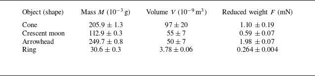
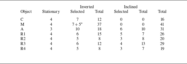


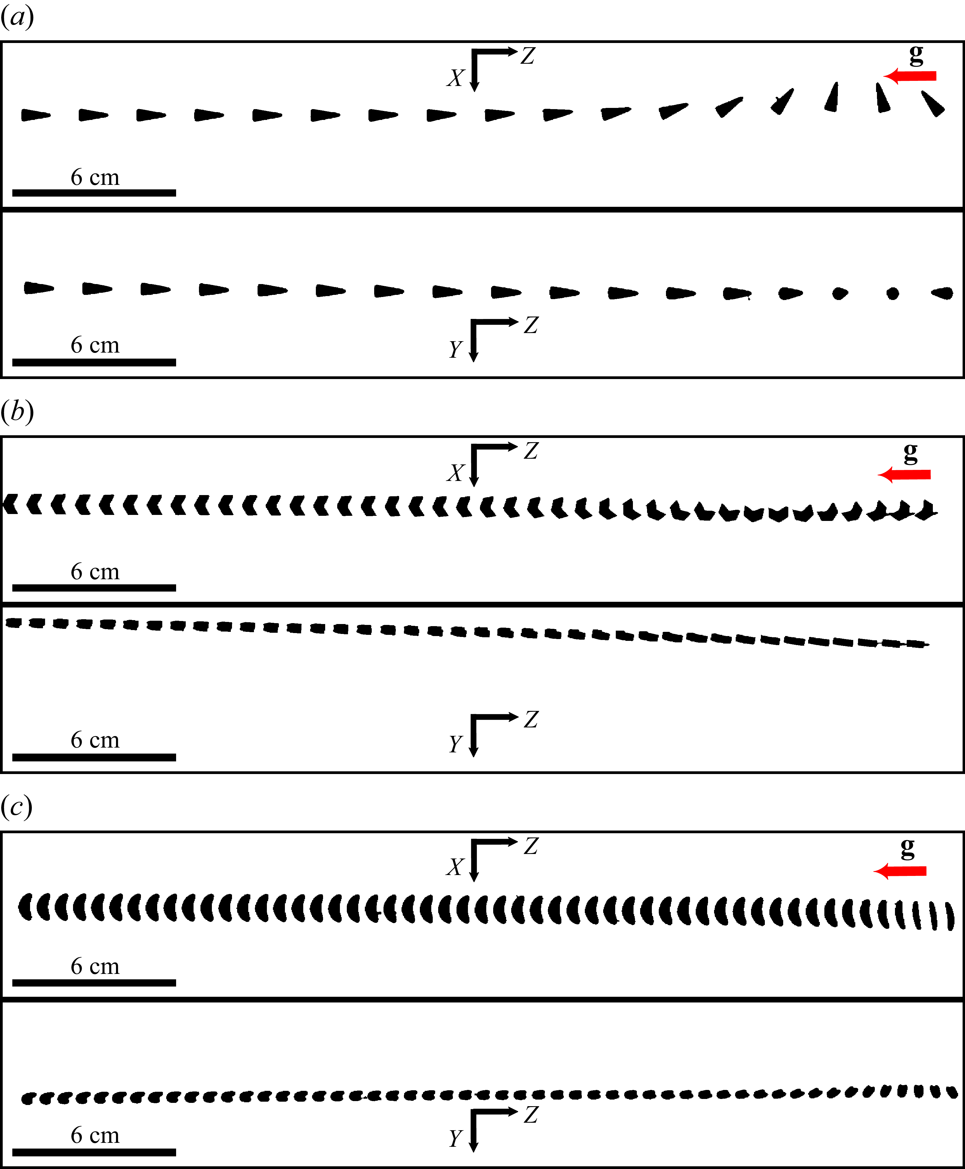
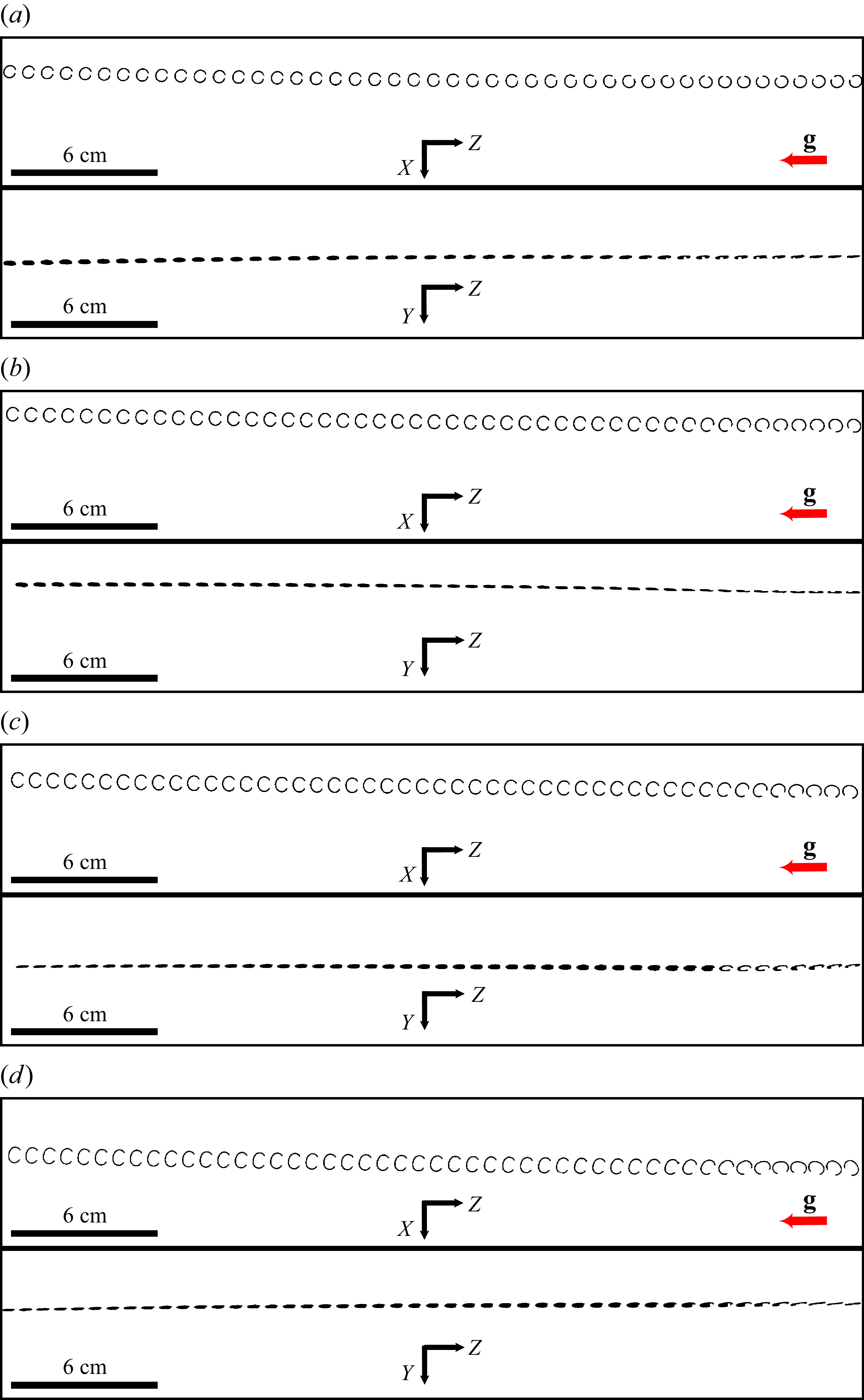


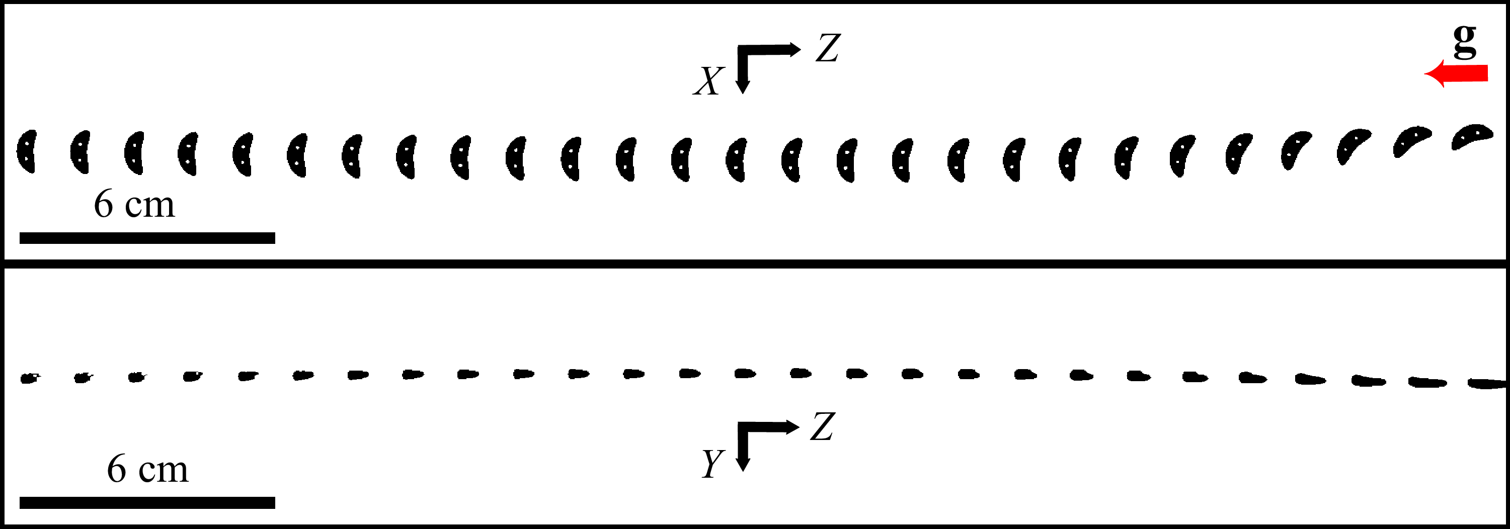
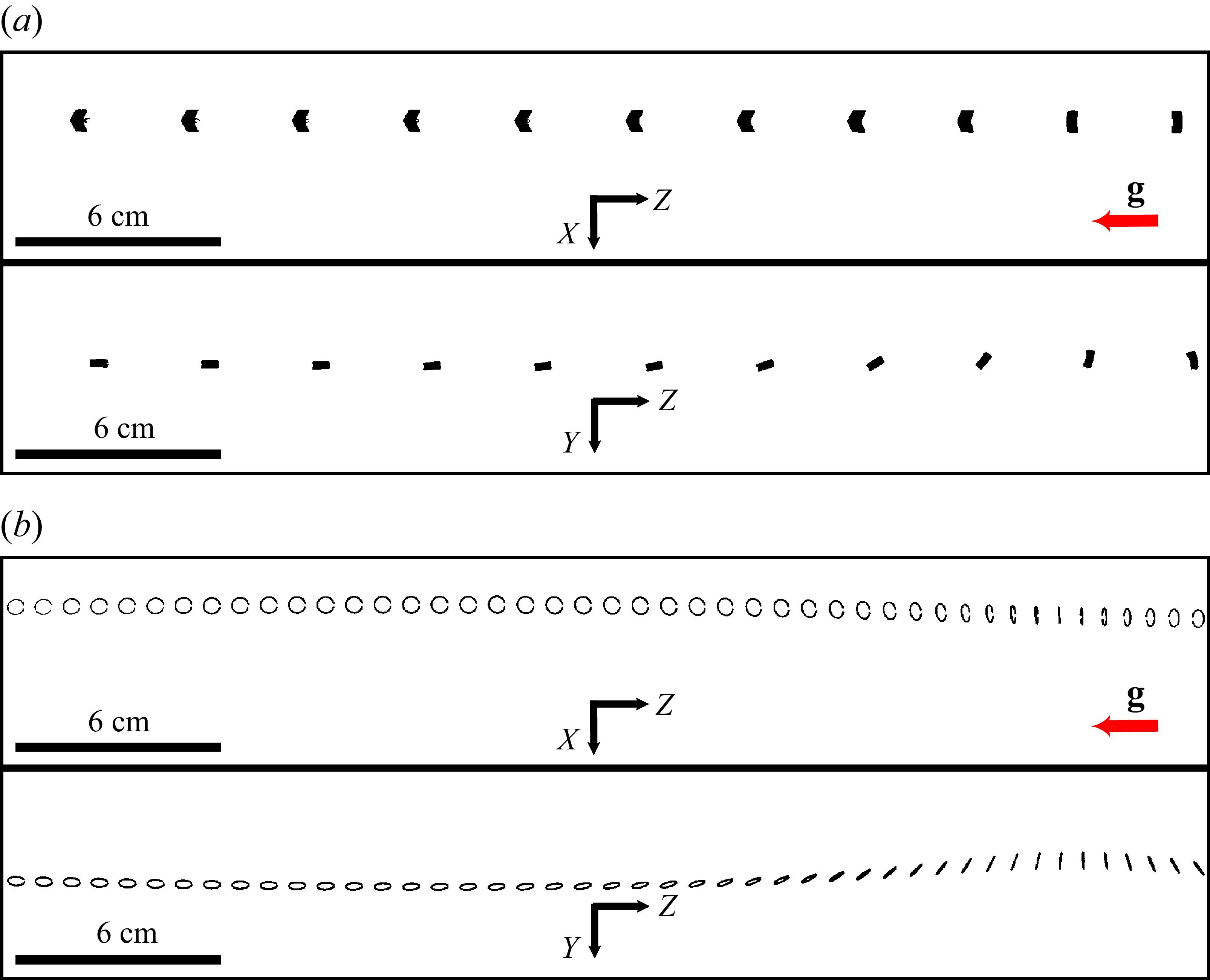
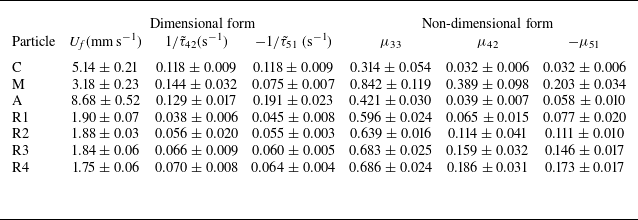


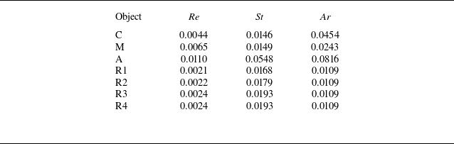


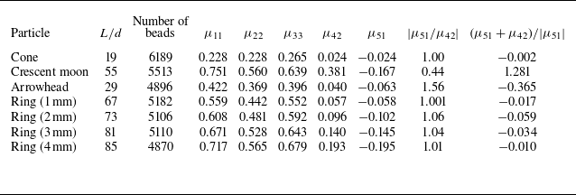
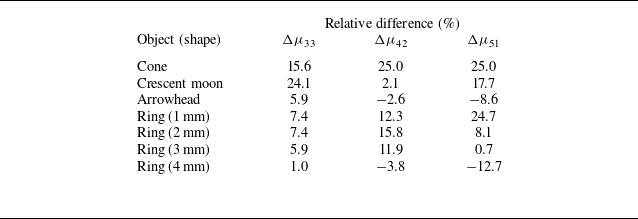


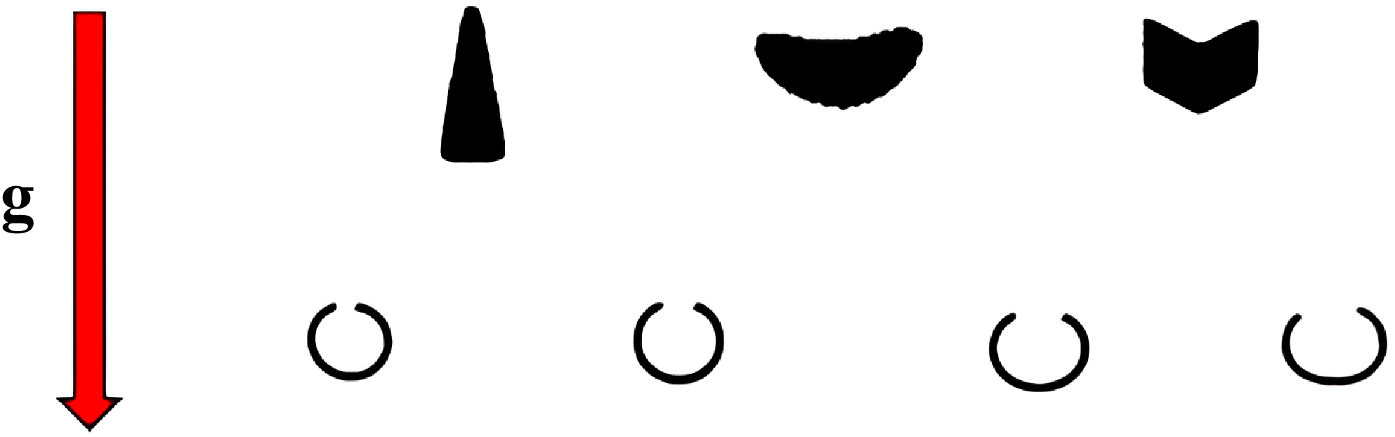

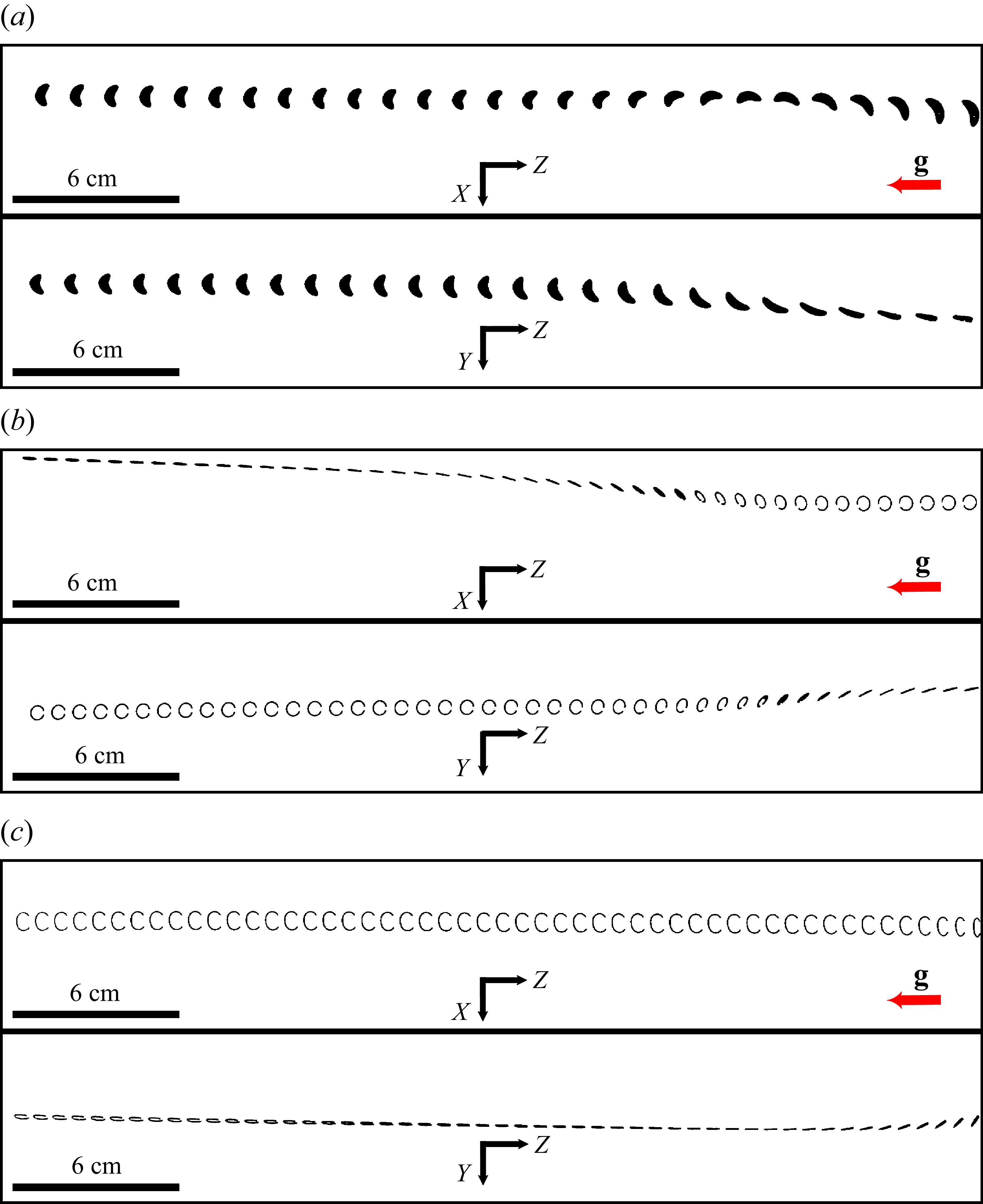
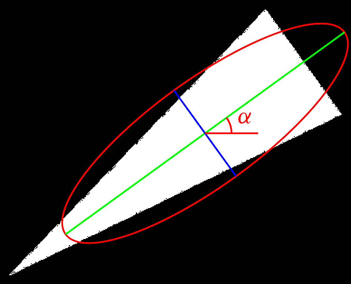

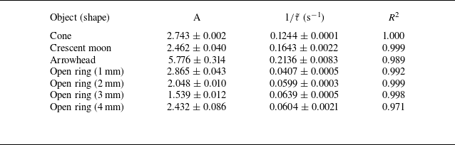


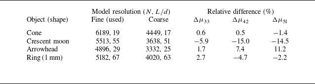


 Open access