2.1. Temperature equation within the ice

The growth rate of ice depends on thermal transfer through the ice governed by conservation of heat within the ice,

(2.1)\begin{equation} \bar{c} \frac{\partial T}{\partial t} = \frac{\partial}{\partial z} \left(\bar{k} \frac{\partial T}{\partial z} \right)- L \frac{\partial X}{\partial t}, \end{equation}

where $T(z,t)$ is the temperature and $X(z,t)$ is the liquid (brine) fraction. The remaining quantities are the thermal properties: $L$ is the volumetric latent heat, $\bar {c}$ is the volumetric heat capacity and $\bar {k}$ is the thermal conductivity. The properties $\bar {c}$ and $\bar {k}$ depend on the relative fraction of the ice that is occupied by solid and liquid. Weighting these properties volumetrically,

(2.2a)\begin{gather} \bar{k} = k_lX + k_s(1-X) \equiv k_s\left[1-X \Delta k \right], \end{gather}

(2.2b)\begin{gather}\bar{c} = c_lX + c_s(1-X) \equiv c_s\left[1-X \Delta c \right], \end{gather}

where a subscript $s$ denotes a property of the solid phase and $l$ denotes a property of the liquid phase. For the final equivalences, we define

(2.3a)\begin{gather} \Delta k = (k_s-k_l)/k_s, \end{gather}

(2.3b)\begin{gather}\Delta c = (c_s-c_l)/c_s. \end{gather}

These are dimensionless measures of the differences between the thermal properties of solid and liquid phases.

The liquid fraction depends on the temperature of the ice as well as its bulk salinity $S$, i.e. the weighted average of the salinity of the solid phase (which is assumed to be zero) and that of the liquid phase $C$. These are related by

(2.4)\begin{equation} S=CX. \end{equation}

We assume that phase change occurs until the system reaches a local thermodynamic equilibrium in which the liquid phase lies at the temperature-dependent freezing point. Thus,

(2.5)\begin{equation} C={-}T/m, \end{equation}

where $m$ is the slope of the freezing point (assumed constant). Hence, by combining with (2.4), we determine the liquid fraction

(2.6)\begin{equation} X = \frac{mS}{-T}, \end{equation}

and by the chain rule

(2.7)\begin{equation} \frac{\partial X}{\partial t} = X\frac{1}{-T}\frac{\partial T}{\partial t} . \end{equation}

Equation (2.7) allows the latent heat term on the right-hand side of (2.1) to be rewritten as an enhanced heat capacity. In particular, we write

(2.8)\begin{equation} c \frac{\partial T}{\partial t} = \kappa_s \frac{\partial}{\partial z} \left(k \frac{\partial T}{\partial z} \right), \end{equation}

where $\kappa _s=k_s/c_s$ is the thermal diffusivity of the solid phase and

(2.9a)\begin{gather} k = 1-X \Delta k , \end{gather}

(2.9b)\begin{gather}c = 1-X \Delta c +\frac{L}{c_s({-}T)} X , \end{gather}

are the dimensionless thermal conductivity and heat capacity respectively. These quantities depend on $T$, so (2.8) is a nonlinear diffusion equation.

2.2. Boundary conditions

In general, suitable boundary conditions for sea-ice evolution require the conservation of heat and salt across the interfaces. Here, we take a simplified approach.

We assume that the top of the ice is held at some temperature $T_B$, the atmospheric temperature. In principle, this temperature could vary in time, in which case $T_B$ would denote the mean (time-averaged) or initial atmospheric temperature. In mushy-layer models, such a fixed temperature boundary condition is commonly used and corresponds physically to a perfectly conducting boundary. In sea-ice models, an energy flux balance is usually used. Hitchen & Wells (Reference Hitchen and Wells2016) showed that such flux balance models can be linearised and expressed as a Robin-type boundary condition involving both $T$ and $\partial T/\partial z$; such boundary conditions could be handled within our modelling framework.

We assume that the bottom of the ice is at the freezing point of seawater $T_0= -m S_0$, where $S_0$ is the salinity of seawater. This introduces a natural temperature scale to the problem

(2.10)\begin{equation} \Delta T \equiv T_0-T_B, \end{equation}

which will be positive for ice growth.

Although (2.8) is a second-order equation and we already have two boundary conditions, we need an extra boundary condition to determine the evolution of the free boundary $h(t)$. Its evolution is determined by a generalised Stefan condition (Kerr et al. Reference Kerr, Woods, Worster and Huppert1989, Reference Kerr, Woods, Worster and Huppert1990). This condition represents the balance of heat fluxes across a narrow boundary layer below the ice–ocean interface

(2.11)\begin{equation} \dot{h}\left[c_l(T_l-T_0) + L (1-X)_{z=h^-}\right] + F_T = k_s \left(k\frac{\partial T}{\partial z}\right)_{z=h^-}, \end{equation}

where $T_l>T_0$ is the temperature of the upper ocean (assumed constant) and $F_T$ is the turbulent heat flux supplied by the ocean. In general, the left-hand side of (2.11) is dominated by the latent heat term, but we retain the sensible heat term $c_l(T_l-T_0)$ as it regularises the boundary condition when the liquid fraction at the interface $X_{z=h^-} =1$.

We introduce a scale for the bulk salinity of sea ice relative to the salinity of the ocean

(2.12)\begin{equation} \hat{S}=S/S_0, \end{equation}

which will lie between 0 and 1 depending on how much the sea ice has desalinated (we discuss the range of $\hat {S}$ in § 2.4). Note that $X_{z=h^-} = \hat {S}$, so $\hat {S}$ can also be thought of as a scale for the liquid fraction.

2.3. Non-dimensionalisation

The growth of ice appears to have no natural length scale. Previous studies of growth in the laboratory have typically used the depth of the tank as a scale (e.g. Kerr et al. Reference Kerr, Woods, Worster and Huppert1990). However, if we are interested in the long-term growth of ice, it makes more sense to use the following scale:

(2.13)\begin{equation} h_\infty = k_s \frac{\Delta T}{F_T}, \end{equation}

which is a scale estimate for the steady-state ice thickness based on estimating the steady-state balance in (2.11). It is important to note that this is a scale estimate, not the actual steady-state thickness. This scale is chosen because we want to investigate how ice growth depends on salinity, so it is convenient to non-dimensionalise with respect to a scale that does not depend on salinity. We report the actual steady-state thickness of the model in § 2.6.

Thus, we introduce a rescaled height ($\hat {h}$) as well as a rescaled time ($\tau$) and distance ($\zeta$) coordinate system:

(2.14a–c)\begin{equation} \hat{h}\equiv \frac{h}{h_\infty}, \quad \tau \equiv \frac{t \kappa_s}{h_\infty^2}, \quad \zeta \equiv \frac{z}{h_\infty \hat{h}}. \end{equation}

The scaling for time is based on thermal diffusion across the steady-state ice thickness. The scaled temperature of ice can be written

(2.15)\begin{equation} \theta=\frac{T-T_B}{\Delta T}, \end{equation}

such that $\theta$ runs between 0 and 1 from the upper (atmospheric) to the lower (oceanic) interface. We denote the scaled cold atmospheric temperature

(2.16)\begin{equation} \theta_B=\frac{-T_B}{\Delta T}, \end{equation}

which is greater than 1 by the definition of $\Delta T$. The effective scaled temperature difference across the ice–ocean boundary layer is

(2.17)\begin{equation} \theta_e=\frac{c_l\left(T_l-T_0\right)}{L}, \end{equation}

where we non-dimensionalise with respect to latent heat because this ratio controls the relative importance of sensible to latent heat fluxes in (2.11).

The Stefan condition (2.11) can be rescaled

(2.18)\begin{equation} \hat{h} \frac{{\rm d}\hat{h}}{{\rm d}\tau} = \frac{1}{\hat{L}} q, \end{equation}

where the scaled latent heat $\hat {L}=L/(c_s\Delta T)$ is often called the Stefan number, and the growth rate factor $q$ is defined by

(2.19)\begin{equation} q = \frac{ \left.k\dfrac{\partial \theta}{\partial \zeta}\right|_{\zeta=1^-} -\hat{h}}{1-\hat{S}+\theta_e}. \end{equation}

Thus,

(2.20)\begin{equation} \frac{{\rm d}}{{\rm d}\tau}\left(\frac{\hat{h}^2 \hat{L}}{2}\right)=q, \end{equation}

so determining $q$ tells us how fast the square of ice thickness changes. We will often refer to $q$, which is the crucial output of our calculations, as the growth rate factor.

Similarly, the temperature equation (2.8) can be written in scaled form

(2.21)\begin{equation} c \hat{h}^2 \frac{\partial \theta}{\partial \tau} - \frac{c \zeta q}{\hat{L}} \frac{\partial \theta}{\partial \zeta} = \frac{\partial}{\partial \zeta} \left(k \frac{\partial \theta}{\partial \zeta} \right), \end{equation}

where scaled versions of the material properties are given by

(2.22a)\begin{gather} X = \hat{S}\frac{\theta_B-1}{\theta_B-\theta} , \end{gather}

(2.22b)\begin{gather}k = 1-X \Delta k , \end{gather}

(2.22c)\begin{gather}c = 1-X \Delta c +\frac{\hat{L}}{\theta_B-\theta} X. \end{gather}

Although (2.21) does not include any direct advective transport, the second term on the left-hand side is a pseudo-advection term proportional to $q$ associated with the changing domain.

2.4. Parameter values and approximations

Six dimensionless parameters characterise the problem. In this section, we give typical values or ranges for these parameters and discuss appropriate approximations. We also recast two parameters to better separate material properties (that are essentially fixed) from quantities that vary depending on environmental conditions. Throughout this section, we use material properties given in table 1 of Rees Jones & Worster (Reference Rees Jones and Worster2014); see references therein for further discussion.

First, the difference between solid and liquid conductivities $\Delta k =1-k_l/k_s\approx 0.76$. This means that the thermal conductivity of ice is about four times higher than that of water, a significant difference. However, various MU-type models use a formula for the thermal conductivity of the form

(2.23)\begin{equation} \bar{k}=k_s + \beta S /T, \end{equation}

where $\beta$ is an empirical constant. By comparing this expression with (2.2a) and (2.6), we see that the MU-type models are equivalent provided $\Delta k =\beta /m k_s$. Particular choices of parameters differ slightly between publications, so, as an example, we consider the default parameter values given in the CICE/Icepack documentation (Hunke et al. Reference Hunke2024a,Reference Hunkeb). These list $\beta =0.13\,{\rm W}\,{\rm m}^{-1}\,{\rm ppt}^{-1}$, $m= 0.054\,{\rm deg}\,{\rm ppt}^{-1}$ and $k_s= 2.03\,{\rm W}\,{\rm m}^{-1}\,{\rm deg}^{-1}$, which combine to give $\Delta k \approx 1.2$. This is physically problematic in the framework of mushy-layer theory because $\Delta k \leq 1$ by definition (2.3a). Indeed, the Icepack documentation casts doubt on the suitability of these parameter values based on experimental results (Hunke et al. Reference Hunke2024b). However, it appears not widely known that these default parameter values are inconsistent with mushy-layer theory. We comment more generally on this issue in the context of large-scale models in § 6.2.

Second, the difference between solid and liquid heat capacities $\Delta c =1-c_l/c_s\approx -1.1$. Equivalently, the heat capacity of water is about double that of ice. This is a significant difference. However, by inspecting (2.22c), we see that the magnitude of $\Delta c$ should be compared with the role of latent heat since both appear multiplied by $X$. Indeed the ratio of the second and third terms is

(2.24)\begin{equation} \frac{\Delta c}{{\hat{L}}/ ({\theta_B-\theta})} \leq \frac{\Delta c \theta_B}{\hat{L}} =\frac{c_s-c_l}{L} ({-}T_B), \end{equation}

where the inequality arises from the fact that $\theta >0$. Even for quite strong cooling, e.g. $T_B=-20\,^\circ {\rm C}$, the ratio in (2.24) is $\lesssim 0.13$. For numerical calculations, we will retain the parameter $\Delta c$. However, it only has a small effect on results and we will neglect it when carrying out analysis to reduce the number of parameters.

Third, the effective ice–ocean temperature difference $\theta _e=c_l(T_l-T_0)/L\ll 1$, because $L/c_l \approx 77\,^\circ {\rm C}$ and any temperature difference is typically less than a degree (and often much smaller). In some mushy-layer models of sea ice, this term still plays an important role, because it regularises the Stefan condition in the case that the liquid fraction $X=1$ at the interface (2.11). However, in our model with a fixed sea-ice salinity, it is reasonable to neglect $\theta _e$ provided $\hat {S}$ is not very close to 1 (which ensures the liquid fraction is not 1 at the interface). Formally, we need $\theta _e \ll 1-\hat {S}$. For numerical calculations, we will use the representative value $T_l-T_0\approx 0.017\,^\circ {\rm C}$, which gives $\theta _e \approx 2\times 10^{-4}$. For analytical calculations, we neglect this term as an excellent approximation.

Fourth, the effective latent heat or Stefan number $\hat {L}=L/(c_s\Delta T) \gg 1$, because $L/c_s \approx 160\,^\circ {\rm C}$ which is much greater than a typical temperature difference across the ice. For example, if $\Delta T \approx 20\,^\circ {\rm C}$, then $\hat {L}\approx 8$. The definition of $\hat {L}$ is convenient for simplifying and analysing the equations. However, one limitation of this formulation is that changing the cold atmospheric temperature $T_B$, which will vary depending on the environmental conditions, changes both $\hat {L}$ and $\theta _B$. Therefore, we introduce an alternative effective latent heat

(2.25)\begin{equation} \hat{L}_0 = \frac{L}{c_s ({-}T_0)} \approx 83, \end{equation}

which, to an excellent approximation, is a fixed material property, because the freezing point of seawater is roughly constant (assuming its salinity does not vary much).

Fifth, the scaled cold atmospheric temperature $\theta _B=-T_B/\Delta T>1$, which ensures that the atmospheric temperature is below the freezing point $T_0$. As $T_B$ approaches $T_0$, the temperature differences $\Delta T$ approaches zero, so $\theta _B$ can be arbitrarily large. Thus, we introduce an alternative parameter

(2.26)\begin{equation} \theta_0=\left(\theta_B-1\right)^{{-}1} \equiv \frac{\Delta T}{-T_0}, \quad \Leftrightarrow \quad \theta_B=1+\theta_0^{{-}1}, \end{equation}

where the equivalence expresses $\theta _0$ in terms of dimensional quantities. In a similar way to $\hat {L}_0$, it is convenient to scale against a fixed quantity. Thus $\theta _0$ varies between 0 (when there is no freezing) and about 9.4 (when $T_B=-20\,^\circ {\rm C}$ and there is strong freezing). Unless otherwise stated, we take a default value $\theta _0\approx 9.4$. Then the Stefan number can be rewritten

(2.27)\begin{equation} \hat{L}=\hat{L}_0 \theta_0^{{-}1}. \end{equation}

Thus, variation in $\theta _0$ should be interpreted as representing variation in the environmental conditions, which in turn controls variation in $\hat {L}$. Combining the default values for $\hat {L}_0$ and $\theta _0$ gives a default value for $\hat {L}\approx 8.3$.

Sixth, the sea-ice salinity $\hat {S}$ defined in (2.12) will lie between 0 and 1. In mushy-layer theory, the salinity is constant across the ice-ocean interface, so $\hat {S}=1$ at the interface. Equivalently, all the salt contained in seawater is initially incorporated into the sea ice as liquid brine inclusions (Notz & Worster Reference Notz and Worster2008). Some laboratory experiments suggest that there is a delay of several hours before desalination begins (Wettlaufer, Worster & Huppert Reference Wettlaufer, Worster and Huppert1997). However, this is a relatively short time period and such a delay was not apparent in the field observations of Notz & Worster (Reference Notz and Worster2008). Within about 12 hours, sea ice appears to lose at least half the salt originally contained in seawater (Notz & Worster Reference Notz and Worster2008; Thomas et al. Reference Thomas, Vancoppenolle, France, Sturges, Bakker, Kaiser and von Glasow2020) so for all but the very initial stages of ice growth, it is reasonable to take $\hat {S}\lesssim 0.5$. For our results, we consider salinities between $\hat {S}=0$ (fresh ice) and $\hat {S}=0.8$ (very salty ice, in dimensional units about 28 ppt, which is much saltier than even very young ice is observed to be) to consider a very broad possible range.

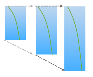
The values of $\Delta k$ and $\Delta c$ ensure that the effective conductivity and heat capacity of sea ice vary considerably in sea ice (figure 1). Saltier ice is less thermally conductive because the liquid fraction is higher. However, saltier ice has a higher heat capacity. The fact that the heat capacity is much greater than 1 reflects the fact that the heat capacity (2.22c) is dominated by latent heat release.

Figure 1.

Depth dependence of the thermal properties of sea ice from atmosphere ($\zeta =0$) to ocean ($\zeta =1$). (a) The thermal conductivity and (b) the heat capacity of sea ice vary considerably with salinity $\hat {S}$. The depth dependence was calculated by assuming that temperature varied linearly with depth ($\theta =\zeta$) in (2.22).

2.5. Dimensional parameter values

The solution of the dimensionless problem only involves the dimensionless parameters introduced previously. However, to convert back to dimensional form, we additionally need the dimensional steady-state thickness estimate $h_\infty$.

In addition to the material properties given in table 1 of Rees Jones & Worster (Reference Rees Jones and Worster2014), we need to specify a value of $F_T$, $T_0$ and $T_B$. We take $F_T=0.0013\,{\rm J}\,{\rm s}^{-1}\,{\rm cm}^{-2}$ and $T_0=-1.9\,^\circ {\rm C}$. This value of $F_T$ is smaller than (about half) that used in Rees Jones & Worster (Reference Rees Jones and Worster2014) and was chosen to achieve a sensible equilibrium thickness, comparable to Maykut & Untersteiner (Reference Maykut and Untersteiner1971). The value of $F_T$ used is within the range observed by Wettlaufer (Reference Wettlaufer1991). For $T_B$, we consider two possible values.

1. (i) For $T_B=-20\,^\circ {\rm C}$, we obtain $\Delta T=18.1\,^\circ {\rm C}$, which gives rise to $h_\infty = 280\,{\rm cm}$ and, hence, a diffusive time scale $h_\infty ^2/\kappa _s = 7.7\times 10^6\,{\rm s}$ (or 89 days).

2. (ii) For $T_B=-10\,^\circ {\rm C}$, we obtain $\Delta T=8.1\,^\circ {\rm C}$, which gives rise to $h_\infty = 130\,{\rm cm}$ and, hence, a diffusive time scale $h_\infty ^2/\kappa _s = 1.5\times 10^6\,{\rm s}$ (or 18 days).

2.6. Equilibrium thickness

The ice grows and reaches an equilibrium (steady-state) thickness $\hat {h}_\infty$ at which the growth rate factor $q=0$. The temperature $\theta =\theta (\zeta )$ alone. By (2.19), we observe that $(k\theta ')(1)=\hat {h}_\infty$. The left-hand side of (2.21) is zero at steady state. Thus, by integrating the right-hand side once and applying the condition at $\zeta =1$, we obtain

(2.28)\begin{equation} \left(1-\hat{S}\Delta k \frac{\theta_B-1}{\theta_B-\theta} \right)\frac{{\rm d} \theta}{{\rm d} \zeta} =\hat{h}_\infty, \end{equation}

where we used (2.22) to express $k$. This is a first-order separable equation with two boundary conditions ($\theta (0)=0$, $\theta (1)=1$) which allows us to determine the unknown parameter $\hat {h}_\infty$. We integrate again and apply the boundary conditions to obtain

(2.29)\begin{align} \hat{h}_\infty&=1-\hat{S}\Delta k\left(\theta_B-1\right)\log \frac{\theta_B}{\theta_B-1}, \nonumber\\ &= 1-\hat{S}\Delta k\theta_0^{{-}1}\log (1+\theta_0), \end{align}

where we used (2.26) to convert from $\theta _B$ to $\theta _0$.

The equilibrium thickness calculated decreases linearly with salinity $\hat {S}$, which is driven by the thermal conductivity difference $\Delta k$. The dependence is also affected by the thermal parameter $\theta _0$. When $\theta _0\ll 1$, we note that $\theta _0^{-1}\log (1+\theta _0)\sim 1 + O(\theta _0)$. This gives $\hat {h}_\infty \approx 1-\hat {S}\Delta k$, an estimate that could be derived using a simple zero-layer type of model of ice in which the temperature field $\theta \approx \zeta$. However, when $\theta _0$ is larger, the sensitivity of equilibrium thickness to salinity is smaller. For example, when $\theta _0\approx 9.4$, the largest value considered in § 2.4, $\theta _0^{-1}\log (1+\theta _0)\approx 0.25$.

2.7. QS approximation

A crucial simplification we can make to the system of equations is to neglect the explicit time-dependence $\partial \theta / \partial \tau$ in the heat equation (2.21). This is a major simplification because it reduces a PDE to an ODE. The resulting equations are still time-dependent because the ice thickness depends on time and this affects the solution via the definition of $q$ in (2.19). For constant boundary conditions and when $\hat {h}\ll 1$, the QS solution is an exact solution of the full PDE. This is sometimes called a similarity solution, an idea used in previous analytical studies (Stefan Reference Stefan1891; Huppert & Worster Reference Huppert and Worster1985; Worster Reference Worster1986). Thus, the QS approximation can be thought of as a generalisation of a similarity solution.

To motivate this approximation, consider the initial phase of ice growth (from an initial thickness of zero). We scaled the equations such that $q=O(1)$ provided $\hat {S}\neq 1$, cf. (2.19). Then, by integrating (2.20),

(2.30)\begin{equation} \hat{h} \propto \sqrt{\frac{2 \tau}{\hat{L}}}, \end{equation}

so the first term in the heat equation (2.21) is a factor of $\tau$ smaller than the second term. Therefore, initially at least, we can guarantee that the explicit time dependence is negligible. Moreover, at later times, the system is likely to be evolving slowly anyway. We will test the practical effects of this approximation later by comparing a full solution of the PDE to the ODE (§ 5.3).

Under the QS approximation, the heat equation (2.21) reduces to a boundary-value problem (BVP)

(2.31a–d)\begin{equation} -\frac{c \zeta q}{\hat{L}} \theta' = (k \theta')', \quad \theta(0)=0, \quad \theta(1)=1, \quad q=\frac{ (k\theta')(1) -\hat{h}}{1-\hat{S}+\theta_e}. \end{equation}

Equation (2.31a) is a second-order ODE with an unknown parameter $q$, hence the three boundary conditions (2.31b–d). The left-hand side of (2.31a) is a pseudo-advection term associated with the change of coordinate system.

The BVP is coupled to an initial-value problem (IVP) for ice thickness (2.20). We define

(2.32)\begin{equation} \hat{y}=\hat{h}^2 \hat{L}/2, \end{equation}

so that the IVP has the simple form

(2.33)\begin{equation} \frac{{\rm d}\hat{y}}{{\rm d} \tau} = q, \quad \hat{y}(0)=0. \end{equation}

The coupled BVP–IVP can be solved very straightforwardly using collocation methods for the BVP (Kierzenka & Shampine Reference Kierzenka and Shampine2001) and Runge–Kutta methods for the IVP. We present an implementation based on the MATLAB bvp4c and ode45 routine, respectively (see the data availability statement for a link to the code). Similar implementations are available in the SciPy library, for example.

3.1. Analytical solution when the Stefan number is large

The parameters of the system (§ 2.4) suggest various approximations that simplify the analysis. We take $\Delta c = \theta _e = 0$ in this subsection and the next. In this subsection, we take $\hat {S}=0$ (fresh ice) and investigate the effect of latent heat in the limit that the Stefan number is large, $\hat {L}\gg 1$. Given that $\hat {S}=0$, the parameters $\Delta k$ and $\theta _B$ do not affect the solution.

The Stefan problem when $\hat {S}=0$ is very well known so we only sketch the solution. The temperature

(3.2)\begin{equation} \theta = \frac{\operatorname{erf} (C \zeta)}{\operatorname{erf} (C)}, \end{equation}

where $C=(q_0/2\hat {L})^{1/2}$ and $q_0 = (2/\sqrt {{\rm \pi} }) C\exp (-C^2)/ \operatorname {erf}(C)$. By eliminating $C$, we obtain an implicit algebraic expression governing $q_0(\hat {L})$. Finally, by taking the limit $\hat {L}\rightarrow \infty$ (in which $C\rightarrow 0$), we obtain the asymptotic estimate

(3.3)\begin{equation} q_0 \sim 1 -\frac{1}{3} \frac{1}{\hat{L}} +\frac{7}{45} \frac{1}{\hat{L}^2} + O(\hat{L}^{{-}3}). \end{equation}

Figure 2 shows that the asymptotic estimate is extremely close to the full numerical solution throughout the parameter range of interest. Indeed, even the leading order estimate $q_0 \sim 1$ has an error of less than about 4 % for $\hat {L}>8$ ($1/\hat {L}<0.125$), the geophysical range of interest identified in § 2.4.

Figure 2.

Dependence of initial growth rate factor $q_0$ on the latent heat $\hat {L}$ calculated numerically and asymptotically (3.3).

The corresponding leading order solution $\theta = \zeta$, i.e. the temperature field is approximately linear through the ice. Thus models that assume a linear temperature profile such as the Semtner zero-layer model (Semtner Reference Semtner1976) are effective provided the latent heat is sufficiently large.

3.2. Analytical solution when the bulk salinity is small

We now extend the analysis to consider small but non-zero bulk salinity by investigating the limit $\hat {S}\ll 1$. We continue to make the assumption that $\hat {L}\gg 1$ but the solution now depends additionally on the parameters $\Delta k$ and $\theta _B$. As we discussed in § 1, one of the major developments in recent sea-ice modelling has been dynamically calculating the bulk salinity. But different models of bulk-salinity evolution seem to have little effect on ice thickness (Griewank & Notz Reference Griewank and Notz2013; Rees Jones & Worster Reference Rees Jones and Worster2014; Worster & Rees Jones Reference Worster and Rees Jones2015). Our goal is to understand the physical reasons for this limited sensitivity and explore how this is manifested in common large-scale sea-ice models.

The key idea is to decompose the temperature field

(3.4)\begin{equation} \theta \sim \zeta + \hat{S} \tilde{\theta}(\zeta) + O(\hat{S}^2,\hat{L}^{{-}1}), \end{equation}

where the perturbation temperature field $\tilde {\theta }$ satisfies a second-order BVP subject to $\tilde {\theta }(0)=\tilde {\theta }(1)=0$. This BVP is obtained by substituting (3.4) into (3.1) and equating terms of the same order in $\hat {S}$ (i.e. we linearise the system in $\hat {S}$).

We give full details in Appendix B. Here we explain the main physical simplifications involved. The liquid fraction $X=\hat {S}(\theta _B-1)/(\theta _B-\theta )$, so to leading order $X$ is proportional to $\hat {S}$ and the temperature field in the denominator can be replaced by $\theta \sim \zeta$. Then the heat capacity ratio on the left-hand side of (3.1a) can be estimated by $c/\hat {L} \sim X/(\theta _B-\zeta )$ for similar reasons. The thermal conductivity $k=1-\Delta k X$ so there is a constant part (which must be retained), and a part that is proportional to $X$, and hence $\hat {S}$, so is retained too. Thus, it is important to consider how thermal conductivity varies with liquid fraction. Finally, the Stefan condition (3.1d) is linearised as follows

(3.5)\begin{equation} q_0=\frac{ (k\theta')(1) }{1-\hat{S} } \sim 1 + \hat{S}\big[1 -\Delta k +\tilde{\theta}'(1)\big]+ O(\hat{S}^2,\hat{L}^{{-}1}). \end{equation}

The term in square brackets includes three terms that control the sensitivity of the growth rate of ice to its salinity.

The first term comes from linearising the denominator of the expression for $q_0$. Physically, this term arises from the latent heat released at the ice–ocean interface. A larger $\hat {S}$ increases the liquid fraction at the interface which reduces the latent heat liberated there which, in turn, increases the growth rate. That is, salty ice tends to grow quicker than fresher ice because there is less latent heat to be conducted away from the growing interface.

The second term comes from linearising the heat flux at the interface: considering the variation in thermal conductivity while retaining the leading order estimate $\theta '(1)\sim 1$. At the interface, $\theta =1$, so the terms involving $\theta _B$ cancel and we are left with a contribution $-\Delta k$. Physically, a higher $\hat {S}$ increases the liquid fraction which reduces the thermal conductivity because liquid water is less conductive than ice. That is, salty ice would tend to grow slower than fresher ice because it is less thermally conductive.

The combination of the first and second terms is consistent with the prediction of a simple zero-layer type of model of ice. Worster & Rees Jones (Reference Worster and Rees Jones2015) discussed the relative insensitivity of ice growth to salinity in terms of the competing effects of thermal conductivity and latent heat growth. Here, we give a clear quantification of that competition. In particular,

(3.6)\begin{equation} \frac{\partial q_0}{\partial \hat{S}} \approx 1 - \Delta k \approx 0.26. \end{equation}

Thus, the overall sensitivity of ice growth to salinity is rather weak because the latent heat and the thermal conductivity dependencies trade-off very strongly, even though individually they vary very strongly with salinity (see figure 1). Mathematically the weak sensitivity arises because the parameter group $1 - \Delta k$ is small. Note that, from the definition of $\Delta k$, we have $1 - \Delta k = k_l/k_s$, so the weak sensitivity occurs in practice because $k_l$ is much smaller than $k_s$.

Furthermore, we identify an additional term, $\tilde {\theta }'(1)$, which is the third term in the bracket of (3.5). This term also comes from linearising the heat flux at the interface, this time considering the changed temperature profile $\tilde {\theta }(\zeta )$ through the ice while fixing the leading order estimate $k=1$. Calculating this term is much more involved as it requires us to solve the BVP for $\tilde {\theta }(\zeta )$.

The total effect of all these terms can be found by calculating $\tilde {\theta }'(1)$ and combining with the other terms (see Appendix B for details). We obtain the asymptotic estimate

(3.7)\begin{equation} q_0 \sim 1+\hat{S}(\theta_B-1)\left[{-}2-(2\theta_B-\Delta k)\log\big(1-\theta_B^{{-}1}\big)\right]+O(\hat{S}^2,\hat{L}^{{-}1}). \end{equation}

This estimate differs from the zero-layer type estimate (3.6) in two main respects. It depends on $\theta _B$ whereas the previous estimate is independent of this parameter. The dependence on $\Delta k$ is also different. The connection between the estimates is clearer if we express equation (3.7) in terms of $\theta _0$ using (2.26), and then rewrite as a sensitivity

(3.8) \begin{align} \frac{\partial q_0}{\partial \hat{S}} &\sim \theta_0^{{-}1}\left[{-}2-(2+2\theta_0^{{-}1}-\Delta k)\log(1+\theta_0)\right]+O(\hat{S},\hat{L}^{{-}1}), \nonumber\\ &\sim \left[1-\Delta k \right]+O(\hat{S},\hat{L}^{{-}1},\theta_0), \end{align}

where the final result follows by taking the limit $\theta _0\rightarrow 0$. Figure 3 shows that the sensitivity of sea-ice growth to salinity varies significantly with the cooling rate $\theta _0$ across the parameter range of interest. The prediction of (3.8) is met at small $\theta _0$. However, for strong cooling conditions when $\theta _0=10$, the growth rate factor is about 40 % smaller than expected at small $\theta _0$, for example. Given that strong cooling (large $\theta _0$) conditions are typical, this newly identified feedback mechanism associated with alteration to the thermal profile is significant.

Figure 3.

Sensitivity of the initial growth rate factor to salinity at small $\hat {S}$ calculated asymptotically in the top line of (3.8). Note that the vertical axis does not begin at zero.

3.3. Numerical results

The asymptotic results were derived by assuming that the salinity of ice was very small $\hat {S}\ll 1$. However, in practice, we are interested in a range of salinities $0\leq \hat {S} \leq 0.8$ as discussed in § 2.4. Therefore, we solve for the initial growth rate factor $q_0$ numerically and compare with the asymptotic predictions

Figure 4 shows the dependence of the initial growth rate factor $q_0$ on salinity $\hat {S}$ according to various different models. The darker blue curves are the main results from our QS model, with $\Delta k =0.74$, which is the best estimate for this parameter (§ 2.4). The corresponding asymptotic predictions agree with the numerical results in the limit of small $\hat {S}$ and are a reasonable approximation for $\hat {S}\lesssim 0.4$. In practice, this corresponds to a dimensional salinity of about 14 ppt, so would be relevant to all but the earliest stages of ice growth. Nevertheless, the numerical results do diverge more sharply at higher salinity, with the growth rate factor exceeding that predicted asymptotically.

Figure 4.

Dependence of initial growth rate factor $q_0$ on the latent heat $\hat {S}$. The solid blue curve corresponds to the full numerical solution with our best estimate of the value of $\Delta k$. This approaches the asymptotic prediction (abbreviated ‘asymp.’ in the legend) as $\hat {S}\rightarrow 0$ (blue dashed curve). The dot-dashed curve shows results for a larger value of $\Delta k$. Lighter, green curves denote the predictions of zero-layer models (solid curve shows the full model while the dashed curve is its asymptotic limit as $\hat {S}\rightarrow 0$). This figure was computed with $\hat {L}=10^{3}$, $\Delta c=\theta _e=0$ to enable direct comparison with the asymptotic theory. These simplifications are tested in figure 5.

Figure 5.

Dependence of the initial growth rate factor on external parameters. (a) Full numerical results with standard material parameter values. (b) Simplified numerical results ($\Delta c = 0$ and $\theta _e=0$). (c) Asymptotic results based on the combination of (3.3) for the dependence on $\hat {L}$ (where $\hat {L}=\hat {L}_0 \theta _0^{-1}$ from (2.27)), and (3.7) for the dependence on $\hat {S}$. Note that we only plot $\theta _0\geq 2$ to focus on the parameter regime of geophysical interest. For smaller values $\theta _0\geq 2$, $q_0$ increases rapidly in both sets of numerical calculations.

We also plot predictions from zero-layer type models in a lighter green colour, both the full calculation (solid) and the asymptotic limit from (3.6) (dashed). These both over-predict the ice growth rate, for the reasons discussed in the previous section. Moreover, the asymptotic limit diverges markedly from the full zero-layer calculation and is a poor approximation for $\hat {S}\gtrsim 0.1$. So even though the asymptotic zero-layer model appears to be a good model, this is coincidental.

The above calculations, including the zero-layer results, were all made with $\Delta k =0.74$. However, in § 2.4, we showed that $\Delta k \approx 1.2$ in MU-type models such as CICE/Icepack (Hunke et al. Reference Hunke2024a,Reference Hunkeb). Thus, we also plot the numerical solution for the higher value of $\Delta k=1.2$. It has a much weaker dependence on $\hat {S}$ because the reduction in growth rate caused by thermal conductivity variation is made stronger.

In summary, all the models we presented agree with the general idea that the sensitivity to salinity is rather weak. The zero-layer model over-predicts the sensitivity while the high-$\Delta k$ model implemented as the default parameter choice in CICE/Icepack tends to under-predict the sensitivity.

In figure 5, we show more completely the dependence of the growth rate factor on the environmentally varying parameters of the system ($\theta _0,\hat {S}$). Comparing panels (a,c), we see that the basic trends found numerically are consistent with the asymptotic analysis across the whole parameter space explored. Comparing panels (a,b) shows that relaxing the assumptions that $\Delta c = 0$ and $\theta _e=0$ makes almost no difference to results, so this was a good assumption across the full parameter regime considered. Thus, the asymptotic analysis (panel c) and the physical mechanisms identified using it (§ 3.2) explain why the initial growth rate varies very weakly with salinity.

To conclude, the weak effect on relative growth rate is not only caused by the relatively low salinity $\hat {S}$ (and, hence, low liquid fraction). For example, even a relatively high salinity ($\hat {S}=0.5$, 50 % of the ocean seawater salinity) corresponds to $q_0-1\approx 0.1$, which is about a 10 % difference in growth rate factor. Thus, the physical mechanisms, first the trade-off in thermal properties (conductivity/latent heat capacity) and second the feedback on temperature profile (analysed asymptotically in § 3.2), are crucial to understanding the role of salinity. In the next section, we investigate how this feeds through to the evolution of ice thickness.

4.1. Effect of ice thickness on the growth rate factor

Under the QS approximation (§ 2.7), the problem of calculating the ice growth rate factor does not depend on the evolution of the ice thickness, only the thickness at a given time. Thus, we now solve the full BVP (2.31) and denote the growth rate factor $q(\hat {h})$. This notation suppresses the dependence on all the material parameters of the system. Note that $q_0=q(\hat {h}=0)$. However, we can not simply take our solutions for $q_0$ and find $q$ by using the Stefan condition (2.31d), because $q$ also appears in the heat equation (2.31a).

Numerically, we observe that the $q(\hat {h})$ varies approximately linearly with $\hat {h}$. Figure 6 shows that this approximation holds very well across the full range of $\hat {h} \in [0,1]$ for parameter values that span the range of interest. While a linear dependence on $\hat {h}$ might be anticipated from (2.31d), the slope is not consistent with $(1-\hat {S}+\theta _e)^{-1}$. This is because the temperature profile itself also changes with $\hat {h}$.

Figure 6.

Dependence of growth rate factor $q$ on the thickness $\hat {h}$ for $\hat {S}=0.3$. The solid blue curve corresponds to the full numerical solution. The dashed light green line shows a first linear approximation given by (4.1). This agrees very well with the full numerical solution. The dot-dashed darker green line shows a second alternative linear approximation $q=q_0 -\hat {h}/(1-\hat {S}+\theta _e)$ which does not agree with the numerical calculation.

Motivated by the observed linear trend in figure 6, we introduce the linear approximation

(4.1)\begin{equation} q(\hat{h}) \approx q_0 - q_1 \hat{h}, \end{equation}

where $q_0$ and $q_1$ depend on the system parameters but not $\hat {h}$. We calculate $q_1$ by computing $q$ at a very small value of $\hat {h}$ to input, along with $q_0$, into a finite difference approximation of the (negative) slope at $\hat {h}=0$.

Figure 7 shows that $q_1$ (panel b) has a similar parametric dependence as $q_0$ (panel a). In particular, $q_1$ increases strongly with salinity. Indeed the dependence of $q_1$ on salinity is stronger than that of $q_0$. The practical implication is that $q(\hat {h})$ can decrease with salinity rather than increase. Figure 7(c) shows that at small $\hat {h}\lesssim 0.4$, the growth rate factor increases with $\hat {S}$ (consistent with the initial growth rate sensitivity found in § 3.2) but for larger $\hat {h}\gtrsim 0.4$, the trend reverses. This reversed trend is consistent with the fact that the equilibrium (steady-state) thickness decreases with salinity (see (2.29) in § 2.6).

Figure 7.

Dependence of the growth rate factor on external parameters. Panels (a,b) show how the constant and linear terms in (4.1), respectively, depend on external parameters. These parameters are the same as the ‘full numerics’ parameters of figure 5. Panel (c) shows the resulting sensitivity of the growth rate factor to salinity at increasing ice thickness. A negative $q$ corresponds to thickness decaying towards its equilibrium state.

Physically the reversal in sensitivity to salinity can be understood by considering the changing relative importance of the different processes that control the sensitivity to salinity. As the ice grows, the growth rate reduces, which reduces the importance of the latent heat sensitivity to salinity (recall that saltier ice grows faster as less latent heat is released by saltier ice). The turbulent ocean heat flux (a constant, independent of salinity) becomes relatively more important. The conductive heat flux reduces, but at a slower rate than the latent heat production reduces. Indeed, as the thickness approaches a steady state (§ 2.6), the latent heat production is negligible and there is a balance between turbulent ocean heat flux and conductive heat flux through the ice. Thus, the fact that the saltier ice is less thermally conductive eventually dominates the overall sensitivity to salinity, such that saltier ice grows slower beyond $\hat {h}\gtrsim 0.4$.

4.2. Ice thickness evolution

As the ice grows $\hat {h}$ increases, so while initially saltier ice grows faster, subsequently saltier ice grows slower. This is a further reason that the sensitivity of ice growth to ice salinity is small. We next investigate the net result by calculating the thickness evolution using (2.33). If the growth rate factor has the simple linear form given by (4.1), then the evolution equation becomes

(4.2)\begin{equation} \frac{{\rm d}\hat{y}}{{\rm d}\tau} = q_0 - (2 q_1^2/\hat{L})^{1/2} \hat{y}^{1/2}, \quad \hat{y}(0)=0, \end{equation}

where we used (2.32) to convert between scaled thickness $\hat {h}$ and scaled squared thickness $\hat {y}$. This is a separable equation and the analytical solution can be written in terms of the product–logarithm function (sometimes called the Lambert $W$-function). This function is defined as the root $w=W$ of $we^w=z$ (the principle value, which satisfies $W\geq -1$, is the relevant root here).

We express the analytical solution in terms of the thickness

(4.3)\begin{equation} \hat{h}= \frac{q_0}{q_1} \left\{1 + W\left[-\exp \left(\frac{-\tau q_1^2}{\hat{L} q_0} -1\right) \right] \right\}. \end{equation}

To the best of the author's knowledge, this expression is a new analytical estimate of the growth trajectory of sea ice. A related expression is given in an implicit form in Worster (Reference Worster2000) and in the PhD thesis Notz (Reference Notz2005) but these earlier expressions are based on a zero-layer model for ice growth.

Figure 8 shows that the thickness is initially proportional to $\tau ^{1/2}$ (see the inset), as is typical for Stefan problems (Worster Reference Worster2000). This comes from taking $q_0\approx 1$ from (3.7), which is valid at small $\hat {S}$ and large $\hat {L}$. However, the thickness diverges markedly from this initial growth even by $\tau =1$. The growth slows and approaches a steady state as $\tau \rightarrow \infty$. The new analytical solution from (4.3) is an excellent approximation to the full numerical solution across the full range of times considered. We plot results for two values of the ice salinity as examples. The initial growth of the saltier ice is slightly faster (but the curves are virtually indistinguishable). At late times, the saltier ice reaches a smaller thickness, consistent with the growth rate factor being a decreasing function of salinity once $\hat {h}\gtrsim 0.4$, as shown in figure 7(c). Thus, the competing sensitivity of growth to salinity at small vs large thickness is an additional reason why the overall ice thickness is relatively insensitive to salinity. For practical purposes, the calculations with different salinities are virtually indistinguishable up to about $\tau \approx 5$, which dimensionally corresponds to a period of at least about 100 days (based on the $T_B=-10\,^\circ {\rm C}$ conversion in § 2.5). This is a remarkable degree of insensitivity in the context of the significant variation in the thermal properties of ice between these salinities.

Figure 8.

Ice thickness evolution calculated according to the numerical model at two different salinities. Dashed curves show the corresponding analytical approximation from (4.3), which are extremely close to the numerical curves. The dot-dashed curve shows an approximation to the initial growth based on $q_0\approx 1$ from (3.3). The inset shows the same data over the initial phase of growth.

5.1. Time-dependent atmospheric temperature

Variable atmospheric conditions are an important factor in sea-ice growth. We adjust the boundary condition at the ice–atmosphere interface. We retain the same non-dimensionalisation but interpret $T_B$ as the long-term average boundary temperature. In dimensionless variables, the only change to the model is that

(5.1)\begin{equation} \theta(0)=\hat{g}(\tau), \end{equation}

where $\hat {g}(\tau )$ represents the time-dependent boundary temperature. Within the QS framework, the growth rate factor only depends on the value of $\hat {g}$ at a particular time, so we denote this dependence $q(\hat {h}, \hat {g})$, again suppressing the dependence on material properties.

Figure 9(a) shows that $q$ decreases approximately linearly with $\hat {g}$. A higher value of $\hat {g}$ corresponds to a higher (warmer) atmospheric temperature so slower ice growth. We introduce the approximation

(5.2)\begin{equation} q(\hat{h}, \hat{g})\approx q_0 - q_1 \hat{h}-q_2 \hat{g}, \end{equation}

where $q_2$ is estimated in an analogous way to $q_1$. A naïve, and rather good estimate of $q_2$ can be obtained by substituting the zero-layer estimate $\theta '(1)=1-\hat {g}$ into (2.31d), which gives

(5.3)\begin{equation} q(0, \hat{g})\approx q_0(1- \hat{g}), \end{equation}

or $q_2\approx q_0$. Figure 9(b) shows that $q_2$ varies only weakly with the external parameters and does so in a similar pattern to $q_0$, although the approximation $q_2\approx q_0$ is not valid uniformly (compare figure 5a).

Figure 9.

(a) Approximately linear dependence of the growth rate factor on $\hat {g}$ for $\hat {h}=0$ and $\hat {S}=0.3$. The first linear model (1) is based on numerical estimation of $q_2$ at small $\hat {g}$ as given by (5.2). The second linear model (2), based on a zero-layer model, is given by (5.3). (b) The full parameter dependence of the slope $q_2$.

We next consider the effect on the trajectory of ice thickness by solving the IVP (2.33) that governs its evolution. The full equation requires numerical solution. However, if we adopt the linearisation (5.2) and take $\hat {g} = \Delta g \hat {g}(\tau )$ where $\Delta g\ll 1$, then we find

(5.4)\begin{equation} \frac{{\rm d}\hat{y}}{{\rm d}\tau} = q_0 - q_1 (2/\hat{L})^{1/2} \hat{y}^{1/2}-q_2 \Delta g \hat{g}(\tau), \quad \hat{y}(0)=0. \end{equation}

This equation can be linearised about the solution for $\Delta g=0$ (i.e. the solution we obtained in § 4.2). We let $\hat {y}=\hat {y}_0 + \Delta g \hat {y}_1$, then

(5.5)\begin{equation} \frac{{\rm d}\hat{y}_1}{{\rm d}\tau} ={-}q_2 \hat{g}(\tau) +q_1 \left(\frac{1}{2\hat{L}}\right)^{1/2} \frac{\hat{y}_1}{ \hat{y}_0^{1/2}} +O(\Delta g) , \quad \hat{y}_1(0)=0. \end{equation}

Note that the quotient is well-behaved in the limit that $\tau \rightarrow 0$. Both the numerator and denominator tend to zero, but by l'Hôpital's rule,

(5.6)\begin{equation} \lim_{\tau \rightarrow 0}\frac{\widehat{y_1}}{ \hat{y}_0^{1/2}} =\lim_{\tau \rightarrow 0}\frac{\hat{y}_1'}{\dfrac{1}{2} \hat{y}_0' \hat{y}_0^{{-}1/2}} =\lim_{\tau \rightarrow 0} \frac{-q_2\hat{g}(0) }{\dfrac{1}{2} q_0 } \hat{y}_0^{1/2} = 0, \end{equation}

where, in the second expression, a prime denotes a derivative with respect to $\tau$. For high latent heat $\hat {L}\gg 1$, the evolution equation for $\hat {y}$ has a simple form:

(5.7)\begin{equation} \frac{{\rm d}\hat{y}_1}{{\rm d}\tau} ={-}q_2 \hat{g}(\tau) +O(\Delta g,\hat{L}^{-{1/2}}) , \quad \hat{y}_1(0)=0. \end{equation}

We use these ideas to propose three solutions to the ice-thickness evolution equation:

1. (i) a numerical solution to the IVP with the full $q(\hat {h}, \hat {g})$;

2. (ii) a numerical solution to the IVP with the linearised form (5.2);

3. (iii) an analytical solution to the IVP based on (5.7).

Figure 10 shows the ice-thickness evolution for a sinusoidal forcing $\hat {g}=\Delta g \sin (\omega \tau )$, where $\omega$ is the angular frequency. While realistic forcing would contain a large spectrum of frequencies, using a simple sinusoidal forcing allows us to test the success of the various approximations we introduced as a function of frequency. For intermediate and high frequency ($\omega =\{10,100\}$, corresponding, roughly, to sub-fortnightly time periods) all the approximations we introduced agree very well with the full numerical solution. (To be more precise, for the $T_B=-10 \,^\circ {\rm C}$ conversion in § 2.5, $\omega =10$ corresponds to a period of 13 days.) For such frequencies, the basic behaviour can be most easily seen by integrating (5.7) which gives

(5.8)\begin{equation} \hat{y}_1 \approx \frac{q_2 \Delta g }{\omega} \left[\cos(\omega t)-1\right]. \end{equation}

The growth rate is anti-phase with the forcing (because a peak in boundary temperature corresponds to a trough in growth rate). Then $\hat {y}$ lags behind the peak in growth rate by a quarter of a cycle. For longer-term variability (e.g. $\omega =1$), the approximations (i)/(ii) agree well. However, there is a more significant departure from (iii). This is expected because $\hat {y}\propto \omega ^{-1}$, so the $O(\hat {L}^{-1/2})$ term neglected in deriving (5.7) will be smaller at high frequency than at low frequency. Similar behaviour has been observed in experimental systems with analogous behaviour (Ding, Wells & Zhong Reference Ding, Wells and Zhong2019).

Figure 10.

The evolution of ice plotted in terms of the squared thickness scale $\hat {y}=\hat {h}^2 \hat {L}/2$ under sinusoidal atmospheric temperature variation $\hat {g}=\Delta g \sin (\omega \tau )$ for $\hat {S}=0.3$. In all panels $\Delta g=0.5$ to allow us to test the success of the approximate solutions beyond the $\Delta g\ll 1$ limit in which they are derived. The panels show different forcing frequencies: (a) low frequency, $\omega =1$; (b) intermediate frequency, $\omega =10$; and (c) high frequency, $\omega =100$. For the latter plots, we restrict the $\tau$ axis range to show a representative part of the solution. Solid blue curve shows the full numerical solution, referred to as (i) in the main text. Dashed green curves show an approximate numerical solution (ii). Dot-dashed dark green curves show an analytical approximation (iii). Solid grey curves show the steady solution equivalent to (4.3).

5.2. Time-dependent salinity

We next investigate the effect of time-dependent salinity on ice growth. The evolution of the salinity profile is complex. Here, we investigate a simple prescribed time-dependent salinity to assess whether or not it has a large effect on ice growth. In particular, we let

(5.9)\begin{equation} \hat{S}(\tau)=\hat{S}_2 + (\hat{S}_1 - \hat{S}_2) \exp(-\tau/\tau_d), \end{equation}

where $\hat {S}_1$ is the initial salinity, $\hat {S}_2$ is the late-time salinity and $\tau _d$ is the desalination time scale over which the salinity evolves. This type of exponential relaxation has been used previously by Vancoppenolle et al. (Reference Vancoppenolle, Fichefet, Goosse, Bouillon, Madec and Morales Maqueda2009) and then used as the ‘slow mode’ of gravity drainage by Turner et al. (Reference Turner, Hunke and Bitz2013). While it does not arise from any particular physical model of desalination, it is a simple functional form to explore.

Figure 11 compares the thickness evolution with a constant salinity (corresponding to either the initial or late-time salinity) with that with an evolving salinity. We look at an extreme example with a high initial salinity $\hat {S}_1=0.9$ and low late-time salinity $\hat {S}_2=0.1$ in order to consider a significant salinity drop. With a relatively rapid desalination time scale $\tau _d\leq 1$, the thickness is extremely close to a fixed salinity model with the prescribed late-time salinity. For longer desalination timescales, the salinity remains higher for longer. The thickness increases more slowly. For extremely long desalination timescales $\tau _d =100,1000$, much longer than the maximum $\tau$ considered, the thickness evolution is close to a fixed salinity with the prescribed initial salinity.

Figure 11.

Ice growth plotted in terms of the squared thickness scale $\hat {y}=\hat {h}^2 \hat {L}/2$ with time-dependent prescribed salinity according to (5.9) with initial salinity $\hat {S}_1=0.9$ and late-time salinity $\hat {S}_2=0.1$. The solid curves correspond to different desalination timescales. The dot-dashed and dashed curves are constant-salinity calculations corresponding to the initial and late-time salinity, respectively. The inset shows the early time behaviour in which all the curves are almost indistinguishable. Close inspection shows that the $\hat {S}=0.1$ dashed curve is lowest early on, while the $\hat {S}=0.9$ dot-dashed curve is lowest at late times.

In practice, we expect ice to desalinate significantly within the 18 days of growth that corresponds in dimensionless units to $\tau =1$ (for the $T_B=-10 \,^\circ {\rm C}$ conversion in § 2.5, and even lower $\tau$ for colder $T_B$), so fixed-salinity models with the late-time salinity are likely to be excellent approximations. A 20-day desalination time scale was previously used for the winter by Vancoppenolle et al. (Reference Vancoppenolle, Fichefet, Goosse, Bouillon, Madec and Morales Maqueda2009). Moreover, all the models give extremely similar results (see the inset plot looking up to $\tau =3$ which corresponds approximately to the first 2 months of growth). Later stages of growth are sensitive to the later-time salinity value.

Although the QS model we developed cannot consider the full dynamic evolution of salinity, it could, in principle, be extended to consider salinity profiles of the separable form

(5.10)\begin{equation} \hat{S} = r(\tau) s(\zeta), \end{equation}

where $r$ and $s$ are given functions. However, caution is needed as the assumptions used to justify the heat equation (2.8) would not be formally valid, as described in Appendix A.

5.3. Non-QS effects

Finally, and most importantly, we consider the limitations of the major simplification introduced in this study, the QS approximation (§ 2.7). For fixed boundary conditions and an initial temperature profile consistent with that calculated within the QS approximation, the full PDE solution is identical to the QS solution. To provide a strong test of the QS solution, we perform experiments with a step change in the atmospheric boundary temperature at a given time $\tau _s$. In dimensional units, we switch from $T_B=-10 \,^\circ {\rm C}$ to $T_B=-20 \,^\circ {\rm C}$. A step change is a more challenging test than the sinusoidal forcing considered in § 5.1. The salinity value used in these experiments was $\hat {S}\approx 0.56$, corresponding to 20 ppt. The non-dimensionalisation of the temperature is based on the initial $T_B$ which gives $\theta _0\approx 4.2$ and $\hat {L}\approx 20$.

Figure 12(a,b) shows an example with a switching time $\tau _s=2$. This corresponds to a dimensional time of 36 days, since we non-dimensionalise with respect to the initial value $T_B=-10 \,^\circ {\rm C}$, which corresponds to a diffusive time scale of 18 days (§ 2.5). The PDE and QS models agree extremely closely. For reference, fixed atmospheric temperature models with the before and after switch temperatures are also plotted. After the switch, the atmospheric temperature is much colder so the ice thickness increases more rapidly. In the QS model, the growth rate increases instantaneously. In the full PDE calculations, the growth rate increases rapidly (but not instantaneously) before catching up with the QS model over a switching lag time $\Delta \tau _s$. After this time, the growth rate of the PDE model is slightly faster than the QS because the thickness is slightly smaller. The absolute differences between the PDE and QS models in terms of thickness are very small.

Figure 12.

Ice growth calculated by the full PDE compared against the QS approximation. Panel (a) shows the evolution of $\hat {y}=\hat {h}^2 \hat {L}/2$ for the PDE and QS models, as well as for two fixed temperature calculations (1, fixed at the initial atmospheric temperature; 2, fixed at the temperature after the switch occurs). The switch occurs at $\tau _s=2$. Panel (b) shows the growth rate for the same example as panel (a). Insets of both panels highlight the behaviour around the switching time. Such experiments are repeated at a series of switching times. Panel (c) shows the results of a series of experiments with $\tau _s=1$, 2, 4, 6 and $10$. It shows the lag $\Delta \tau _s$ before the growth rate of the PDE catches up with that of the QS model. It also shows the maximum absolute difference in $\hat {y}$ after the switching time between the PDE and QS models denoted $\Delta y_s$. Linear fits to the data are shown.

The switching lag depends on the thickness around the time the switch occurs. Figure 12(c) shows the results of a series of experiments at different switching times. We observe that the lag is proportional to the value of the square of the ice thickness at the switching time, i.e. $\Delta \tau _s \propto \hat {y}(\tau _s)$. This is because the lag corresponds to the time it takes for the cooling at the ice–atmosphere interface to diffuse across the full depth of the ice to the ice–ocean interface. A similar diffusive lag was observed experimentally by Ding et al. (Reference Ding, Wells and Zhong2019). In our dimensionless units, $\Delta \tau _s \propto [\hat {h}(\tau _s)]^2 \propto \hat {y}(\tau _s)$. During this period of slower growth for the PDE model, slightly less ice grows. We denote the maximum absolute difference in $\hat {y}$ between the PDE and QS models as $\Delta y_s$. We observe that $\Delta \hat {y}_s \propto \Delta \tau _s \propto \hat {y}(\tau _s)$. The first proportionality assumes that $d\hat {y}/d\tau$ is approximately independent of switching time. While this is only an approximation, across the range considered in figure 12(c), the discrepancy is within about $\pm 15$ %, so the dot-dashed linear fit matches the calculated $\Delta y_s$ well. Thus, although the lag increases with switching time, and the square thickness change $\Delta \hat {y}_s$ increases too, the proportionate change $\Delta \hat {y}_s/\hat {y}(\tau _s)$ does not increase. Therefore, the QS model remains an effective approximation to the PDE model for any switching time.

This was a strong test of the QS model. In practice, changes in atmospheric temperature will occur in both directions (not just a sudden cooling), which would partly offset each other. Furthermore, more realistic changes would occur more gradually than the instantaneous switch tested here. Thus, it is reasonable to expect the QS model to perform even better under more realistic forcing scenarios.