


1 Introduction
The majority of rocket-related problems featured in the literature rely on reduced-order models that idealize solid propellant motors by considering that their bulk gaseous motion may be suitably represented by the internal flow field evolving within porous channels and tubes. In such idealizations, the effects of compressibility may be either retained or dismissed, depending on the gas injection speed and the nozzleless chamber length. While the incompressible motion is relatively well understood (Taylor Reference Taylor1956; Culick Reference Culick1966; Majdalani & Akiki Reference Majdalani and Akiki2010), recent advances have enabled us to account for the presence of arbitrary headwall injection (Majdalani & Saad Reference Majdalani and Saad2007b ; Saad & Majdalani Reference Saad and Majdalani2009), wall regression (Majdalani, Vyas & Flandro Reference Majdalani, Vyas and Flandro2002; Zhou & Majdalani Reference Zhou and Majdalani2002), grain taper (Saad, Sams & Majdalani Reference Saad, Sams and Majdalani2006; Sams, Majdalani & Saad Reference Sams, Majdalani and Saad2007), variable cross-section (Kurdyumov Reference Kurdyumov2006), headwall singularity (Chedevergne, Casalis & Féraille Reference Chedevergne, Casalis and Féraille2006), viscous effects (Majdalani & Akiki Reference Majdalani and Akiki2010), and stability (Chedevergne, Casalis & Majdalani Reference Chedevergne, Casalis and Majdalani2012). Furthermore, flow approximations exhibiting smoother or steeper profiles than the cold flow equilibrium state have been studied in connection with their energy content by Majdalani & Saad (Reference Majdalani and Saad2007a ) and Saad & Majdalani (Reference Saad and Majdalani2008). In what concerns compressible flow effects, these have been first investigated by Traineau, Hervat & Kuentzmann (Reference Traineau, Hervat and Kuentzmann1986) in the context of two-dimensional porous tubes and channels with sidewall injection. Using either nitrogen or air as the working substance, these investigators have reported rich characteristics of the spatially developing motion, which has been shown to depict appreciable steepening beyond the Taylor–Culick baseline (Taylor Reference Taylor1956; Culick Reference Culick1966). In the downstream sections of the domain, compressibility intensified to the extent of producing noticeably flattened mean-flow profiles. These observations were further supported by numerical simulations attributed to Beddini (Reference Beddini1986), Baum, Levine & Lovine (Reference Baum, Levine and Lovine1988), Liou & Lien (Reference Liou and Lien1995), and Apte & Yang (Reference Apte, Yang, Yang, Brill and Ren2000, Reference Apte and Yang2001). They were also studied by Gany & Aharon (Reference Gany and Aharon1999) and King (Reference King1987) in the context of nozzleless rocket motors. While the former group explored the merits of a one-dimensional theoretical model, the latter employed a pseudo-two-dimensional numerical approach. Given the relevance of an accurate mean-flow description to the study of hydrodynamic instability in simulated rocket motors, the problem was revisited by Venugopal, Najjar & Moser (Reference Venugopal, Najjar and Moser2001) and, in complementary work, by Wasistho, Balachandar & Moser (Reference Wasistho, Balachandar and Moser2004). As a windfall, the compressible solutions engendered in these studies became valuable resources in the limiting process verification of Navier–Stokes solvers (Wasistho et al. Reference Wasistho, Haselbacher, Najjar, Tafti, Balachandar and Moser2002; Najjar et al. Reference Najjar, Haselbacher, Ferry, Wasistho, Balachandar and Moser2003). This was partly caused by the obstacles placed against the acquisition of rocket-related experimental data and, partly, because of the harsh, intrusion-resistant medium arising in highly pressurized and reactive chambers.
Among the analytical techniques that have been applied to this problem, the first may be the Prandtl–Glauert expansion (Shapiro Reference Shapiro1953). In fact, a variant of this technique was used by Traineau et al. (Reference Traineau, Hervat and Kuentzmann1986), who introduced, in a precursor to the present study, a rotational and compressible integral equation, which can be solved in a planar, two-dimensional, and viscous-free setting. In the same context, two related extensions appeared, given by Balakrishnan, Liñan & Williams (Reference Balakrishnan, Liñan and Williams1991) and Akiki & Majdalani (Reference Akiki and Majdalani2012). In addition to their elegant theoretical and numerical work, Traineau and co-workers have furnished a collection of experimental data based on cold flow measurements with air as the sidewall injectant. Moreover, these investigators have implemented judicious scaling arguments to justify the dismissal of the radial momentum equation, thereby reducing the remaining momentum, mass, energy, ideal gas, and isentropic state relations to a single integral expression that can be numerically solved for the pressure distribution. This was accomplished by relating the pressure and wall mass flux through the Saint-Robert power law, and by showing that the Abel integral equation that precipitates can be inverted analytically in the case for which $2(2-\unicode[STIX]{x1D6FE})/(\unicode[STIX]{x1D6FE}-1)$
takes on an integer value.
$2(2-\unicode[STIX]{x1D6FE})/(\unicode[STIX]{x1D6FE}-1)$
takes on an integer value.
The second analytical approach used in this context refers to a variant of the Rayleigh–Janzen expansion. The technique in question is based on small parameter perturbations in the square of the wall injection Mach number. The Rayleigh–Janzen expansion was first applied by Majdalani (Reference Majdalani2007) in the treatment of the axisymmetric porous cylinder and then by Maicke & Majdalani (Reference Maicke and Majdalani2008) in the planar flow analogue. The axisymmetric analysis led to two closed-form solutions: one exact, satisfying all first principles, and one approximate, which proved to be practically equivalent. In contrast, the planar effort gave rise to a single compact expression satisfying all physical requirements. At the outset, both streamwise and wall-normal velocity profiles could be readily calculated, in addition to the critical length required to achieve sonic conditions. In both configurations, the effort led to the identification of the sonic distance as the appropriate length scale which, when inserted into the solution, would promote a self-similar, parameter-independent behaviour for all wall Mach numbers. It also disclosed a simple criterion that could help to determine the relative effects of compressibility and the corresponding centreline amplification during flow development. By eliminating the need to calculate the base flow over the fluid domain, the resulting expressions opened up new avenues for conducting parametric trade analyses.
In complementing ongoing efforts to obtain closed-form solutions for the flow in porous cylinders, it is the purpose of this study to extend the integral formulation developed initially by Traineau et al. (Reference Traineau, Hervat and Kuentzmann1986) and later reconstructed by Balakrishnan, Liñan & Williams (Reference Balakrishnan, Liñan and Williams1992). Our objective is to produce a complete pseudo-two-dimensional approximation that would not be limited to homentropic flow conditions, and that would obviate the need for numerical integration, at least in some well-defined cases of interest. The resulting formulation would also permit direct comparisons to available one- and two-dimensional closed-form representations.
The following summary outlines the organization of this paper. Section 2 describes the mathematical derivation of the integral formulation as well as the numerical approach used. In § 3, discussions of the numerical results are presented. Afterwards, a mathematical approach to achieve an exact solution of the governing integral equation is described in § 4. Then, in § 5, the approach is used in an example flow with oscillatory wall injection. Finally, conclusions are summarized in § 6.
2 Mathematical model
2.1 Geometry
We consider the steady, inviscid flow of an ideal gas in a cylinder of length $L_{0}$
and radius
$L_{0}$
and radius $a$
. A schematic diagram of the problem is given in figure 1. The origin of the coordinate system is located at the centre of the headwall. The motion is taken to be axisymmetric and swirl-free, which enables us to limit our investigation to the upper half
$a$
. A schematic diagram of the problem is given in figure 1. The origin of the coordinate system is located at the centre of the headwall. The motion is taken to be axisymmetric and swirl-free, which enables us to limit our investigation to the upper half $r-x$
portion of the porous chamber. Note that
$r-x$
portion of the porous chamber. Note that $\unicode[STIX]{x1D713}$
represents a streamline and
$\unicode[STIX]{x1D713}$
represents a streamline and $\unicode[STIX]{x1D709}$
denotes the axial distance from the headwall to the point where a streamline is generated at the sidewall, i.e. the tip of a streamline.
$\unicode[STIX]{x1D709}$
denotes the axial distance from the headwall to the point where a streamline is generated at the sidewall, i.e. the tip of a streamline.
Sketch of a slender rocket motor (a) of length $L_{0}$
and radius
$L_{0}$
and radius $a$
, modelled as a right-cylindrical porous chamber (b) with an imposed sidewall injection velocity
$a$
, modelled as a right-cylindrical porous chamber (b) with an imposed sidewall injection velocity $U_{w}(x)$
.
$U_{w}(x)$
.

2.2 Formulation
A solid rocket motor is often idealized as a slender, elongated chamber with sidewall injection. Under the assumption of low chamber aspect ratio, $a/L_{0}\ll 1$
, the system’s conservation equations may be conveniently reduced to the following set:
$a/L_{0}\ll 1$
, the system’s conservation equations may be conveniently reduced to the following set:
 $$\begin{eqnarray}\displaystyle & \displaystyle \frac{\unicode[STIX]{x2202}(\unicode[STIX]{x1D70C}ur)}{\unicode[STIX]{x2202}x}+\frac{\unicode[STIX]{x2202}(\unicode[STIX]{x1D70C}vr)}{\unicode[STIX]{x2202}r}=0\quad \text{(compressible continuity)}, & \displaystyle\end{eqnarray}$$
 $$\begin{eqnarray}\displaystyle & \displaystyle \unicode[STIX]{x1D70C}u\frac{\unicode[STIX]{x2202}u}{\unicode[STIX]{x2202}x}+\unicode[STIX]{x1D70C}v\frac{\unicode[STIX]{x2202}u}{\unicode[STIX]{x2202}r}=-\frac{\unicode[STIX]{x2202}p}{\unicode[STIX]{x2202}x}\quad \text{(axial momentum)}, & \displaystyle\end{eqnarray}$$
 $$\begin{eqnarray}\displaystyle & \displaystyle \frac{\unicode[STIX]{x2202}p}{\unicode[STIX]{x2202}r}=0\quad \text{(radial momentum)} & \displaystyle\end{eqnarray}$$
and
 $$\begin{eqnarray}\unicode[STIX]{x1D70C}u\frac{\unicode[STIX]{x2202}}{\unicode[STIX]{x2202}x}\left(c_{p}T+\frac{u^{2}}{2}\right)+\unicode[STIX]{x1D70C}v\frac{\unicode[STIX]{x2202}}{\unicode[STIX]{x2202}r}\left(c_{p}T+\frac{u^{2}}{2}\right)=0\quad \text{(energy)},\end{eqnarray}$$
where $u$
and
$u$
and $v$
denote the velocities in the
$v$
denote the velocities in the $x$
and
$x$
and $r$
directions, respectively. Similarly,
$r$
directions, respectively. Similarly, $p$
,
$p$
, $T$
and
$T$
and $\unicode[STIX]{x1D70C}$
designate the pressure, temperature, and density. Note that pressure variations have been discounted in the radial direction due to the chamber’s low aspect ratio. Knowing that
$\unicode[STIX]{x1D70C}$
designate the pressure, temperature, and density. Note that pressure variations have been discounted in the radial direction due to the chamber’s low aspect ratio. Knowing that $x$
scales with
$x$
scales with $L_{0}$
and
$L_{0}$
and $r$
scales with
$r$
scales with $a$
, an examination of the continuity equation establishes that
$a$
, an examination of the continuity equation establishes that $u$
must be of the order of
$u$
must be of the order of $vL_{0}/a$
. Assuming
$vL_{0}/a$
. Assuming $a\ll L_{0}$
, we get
$a\ll L_{0}$
, we get $u\gg v$
, and so the magnitude of the total velocity can be reduced to
$u\gg v$
, and so the magnitude of the total velocity can be reduced to $V^{2}\approx u^{2}$
. In turn, the term of order
$V^{2}\approx u^{2}$
. In turn, the term of order $O(v^{2})$
disappears from (2.4). Furthermore, the gas may be taken to be ideal and calorically perfect, thus warranting a constant
$O(v^{2})$
disappears from (2.4). Furthermore, the gas may be taken to be ideal and calorically perfect, thus warranting a constant $c_{p}$
. The resulting ideal gas law may be expressed in terms of the ratio of specific heats,
$c_{p}$
. The resulting ideal gas law may be expressed in terms of the ratio of specific heats, $\unicode[STIX]{x1D6FE}$
, using
$\unicode[STIX]{x1D6FE}$
, using
 $$\begin{eqnarray}p=\frac{\unicode[STIX]{x1D6FE}-1}{\unicode[STIX]{x1D6FE}}c_{p}\unicode[STIX]{x1D70C}T.\end{eqnarray}$$
From compressible theory, one can straightforwardly show that the isentropic relation, $\unicode[STIX]{x1D719}=T/p^{[(\unicode[STIX]{x1D6FE}-1)/\unicode[STIX]{x1D6FE}]}$
, remains constant along a streamline.
$\unicode[STIX]{x1D719}=T/p^{[(\unicode[STIX]{x1D6FE}-1)/\unicode[STIX]{x1D6FE}]}$
, remains constant along a streamline.
2.3 Boundary conditions
The physical requirements at the sidewall, headwall, and centreline may be written as:
 $$\begin{eqnarray}\left.\begin{array}{@{}ll@{}}u(x,a)=0 & \text{(no slip at sidewall)},\\ u(0,r)=0 & \text{(no headwall injection)},\\ v(x,a)=-U_{w}(x) & \text{(radial sidewall injection)},\\ v(x,0)=0 & \text{(no crossflow at the centreline)},\\ T(x,a)=T_{w}(x) & \text{(sidewall temperature)},\\ p(0)=p_{0} & \text{(headwall pressure)},\end{array}\right\}\end{eqnarray}$$
where the subscript $w$
refers to conditions at the wall. It may be helpful to remark that the pressure
$w$
refers to conditions at the wall. It may be helpful to remark that the pressure $p=p(x)$
will be permitted to evolve only with respect to
$p=p(x)$
will be permitted to evolve only with respect to $x$
due to the slender motor assumption,
$x$
due to the slender motor assumption, $a/L_{0}\ll 1$
, and in view of (2.3). This is contrary to the temperature and velocity profiles, which will be allowed to retain their two-dimensional character with respect to both
$a/L_{0}\ll 1$
, and in view of (2.3). This is contrary to the temperature and velocity profiles, which will be allowed to retain their two-dimensional character with respect to both $x$
and
$x$
and $r$
.
$r$
.
2.4 Streamfunction transformation
For axisymmetric motions, the Stokes streamfunction may be defined as
 $$\begin{eqnarray}\displaystyle & \displaystyle \frac{\unicode[STIX]{x2202}\unicode[STIX]{x1D713}}{\unicode[STIX]{x2202}r}=\unicode[STIX]{x1D70C}ur, & \displaystyle\end{eqnarray}$$
 $$\begin{eqnarray}\displaystyle & \displaystyle \frac{\unicode[STIX]{x2202}\unicode[STIX]{x1D713}}{\unicode[STIX]{x2202}x}=-\unicode[STIX]{x1D70C}vr. & \displaystyle\end{eqnarray}$$
Given that the stagnation enthalpy, $(c_{p}T+(1/2)u^{2})$
, remains invariant along a streamline, one can put
$(c_{p}T+(1/2)u^{2})$
, remains invariant along a streamline, one can put
 $$\begin{eqnarray}T(x,\unicode[STIX]{x1D713})+u^{2}(x,\unicode[STIX]{x1D713})/(2c_{p})=T_{w}(\unicode[STIX]{x1D713}),\end{eqnarray}$$
where $T_{w}(\unicode[STIX]{x1D713})$
is the total, stagnation temperature along a streamline. Then, in view of
$T_{w}(\unicode[STIX]{x1D713})$
is the total, stagnation temperature along a streamline. Then, in view of $\unicode[STIX]{x1D719}$
, the isentropic pressure–temperature relation may be expressed as
$\unicode[STIX]{x1D719}$
, the isentropic pressure–temperature relation may be expressed as
 $$\begin{eqnarray}T(x,\unicode[STIX]{x1D713})/[p(x)]^{(\unicode[STIX]{x1D6FE}-1)/\unicode[STIX]{x1D6FE}}=T_{w}(\unicode[STIX]{x1D713})/[p_{w}(\unicode[STIX]{x1D713})]^{(\unicode[STIX]{x1D6FE}-1)/\unicode[STIX]{x1D6FE}}.\end{eqnarray}$$
Realizing that all streamlines originate through surface injection at $r=a$
, equation (2.8) may be readily evaluated at the sidewall. This may be performed using the ideal gas expression for the density. Subsequent integration in the axial direction yields
$r=a$
, equation (2.8) may be readily evaluated at the sidewall. This may be performed using the ideal gas expression for the density. Subsequent integration in the axial direction yields
 $$\begin{eqnarray}\unicode[STIX]{x1D713}=\frac{a\,\unicode[STIX]{x1D6FE}}{(\unicode[STIX]{x1D6FE}-1)c_{p}}\int _{0}^{\unicode[STIX]{x1D709}}[U_{w}(x)p(x)/T_{w}(x)]\,\text{d}x.\end{eqnarray}$$
As depicted in figure 1, $\unicode[STIX]{x1D709}$
denotes the distance from the headwall to the point where the streamline intersects with the sidewall. Because a unique value of
$\unicode[STIX]{x1D709}$
denotes the distance from the headwall to the point where the streamline intersects with the sidewall. Because a unique value of $\unicode[STIX]{x1D713}$
may be associated with a given
$\unicode[STIX]{x1D713}$
may be associated with a given $\unicode[STIX]{x1D709}$
, the independent variables may be shifted from
$\unicode[STIX]{x1D709}$
, the independent variables may be shifted from $(x,\unicode[STIX]{x1D713})$
to
$(x,\unicode[STIX]{x1D713})$
to $(x,\unicode[STIX]{x1D709})$
. In this new coordinate system, equations (2.9) and (2.10) may be written as
$(x,\unicode[STIX]{x1D709})$
. In this new coordinate system, equations (2.9) and (2.10) may be written as
 $$\begin{eqnarray}\displaystyle & \displaystyle T(x,\unicode[STIX]{x1D709})+u^{2}(x,\unicode[STIX]{x1D709})/(2c_{p})=T_{w}(\unicode[STIX]{x1D709}), & \displaystyle\end{eqnarray}$$
 $$\begin{eqnarray}\displaystyle & \displaystyle T(x,\unicode[STIX]{x1D709})/[p(x)]^{(\unicode[STIX]{x1D6FE}-1)/\unicode[STIX]{x1D6FE}}=T_{w}(\unicode[STIX]{x1D709})/[p_{w}(\unicode[STIX]{x1D709})]^{(\unicode[STIX]{x1D6FE}-1)/\unicode[STIX]{x1D6FE}}=T_{w}(\unicode[STIX]{x1D709})/[p(\unicode[STIX]{x1D709})]^{(\unicode[STIX]{x1D6FE}-1)/\unicode[STIX]{x1D6FE}}. & \displaystyle\end{eqnarray}$$
Next, the expression for the streamfunction given by (2.11) may be substituted into (2.7) and then integrated in the radial direction. This enables us to deduce the coordinate $r$
associated with a given axial position
$r$
associated with a given axial position $x$
and streamline emanating from
$x$
and streamline emanating from $\unicode[STIX]{x1D709}$
. We get
$\unicode[STIX]{x1D709}$
. We get
 $$\begin{eqnarray}r^{2}=2a\int _{0}^{\unicode[STIX]{x1D709}}\left[\frac{T(x,\unicode[STIX]{x1D709}^{\prime })}{p(x)u(x,\unicode[STIX]{x1D709}^{\prime })}\right]\left[\frac{U_{w}(\unicode[STIX]{x1D709}^{\prime })p(\unicode[STIX]{x1D709}^{\prime })}{T_{w}(\unicode[STIX]{x1D709}^{\prime })}\right]\text{d}\unicode[STIX]{x1D709}^{\prime }.\end{eqnarray}$$
We can also replace the variables $u$
and
$u$
and $T$
using (2.12) and (2.13) to deduce an expression solely in terms of the pressure. This operation yields
$T$
using (2.12) and (2.13) to deduce an expression solely in terms of the pressure. This operation yields
 $$\begin{eqnarray}r^{2}=2a\int _{0}^{\unicode[STIX]{x1D709}}\left[\frac{p(\unicode[STIX]{x1D709}^{\prime })}{p(x)}\right]^{1/\unicode[STIX]{x1D6FE}}\left[1-\left[\frac{p(x)}{p(\unicode[STIX]{x1D709}^{\prime })}\right]^{(\unicode[STIX]{x1D6FE}-1)/\unicode[STIX]{x1D6FE}}\right]^{-1/2}\frac{U_{w}(\unicode[STIX]{x1D709}^{\prime })}{\sqrt{2c_{p}T_{w}(\unicode[STIX]{x1D709}^{\prime })}}\,\text{d}\unicode[STIX]{x1D709}^{\prime }.\end{eqnarray}$$
At this juncture, we are ready to evaluate (2.15) knowing that $\unicode[STIX]{x1D709}=x$
at
$\unicode[STIX]{x1D709}=x$
at $r=a$
. We find
$r=a$
. We find
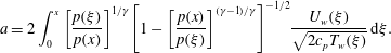 $$\begin{eqnarray}a=2\int _{0}^{x}\left[\frac{p(\unicode[STIX]{x1D709})}{p(x)}\right]^{1/\unicode[STIX]{x1D6FE}}\left[1-\left[\frac{p(x)}{p(\unicode[STIX]{x1D709})}\right]^{(\unicode[STIX]{x1D6FE}-1)/\unicode[STIX]{x1D6FE}}\right]^{-1/2}\frac{U_{w}(\unicode[STIX]{x1D709})}{\sqrt{2c_{p}T_{w}(\unicode[STIX]{x1D709})}}\,\text{d}\unicode[STIX]{x1D709}.\end{eqnarray}$$
Equation (2.16) is thus reduced to one unknown, which is the pressure distribution in the axial direction.
2.5 Integral formulation with no pressure dependence
The dimensionless variables $P(X)$
,
$P(X)$
, $X$
and
$X$
and $\unicode[STIX]{x1D701}$
may be conveniently introduced to simplify the analysis. These are defined according to
$\unicode[STIX]{x1D701}$
may be conveniently introduced to simplify the analysis. These are defined according to
 $$\begin{eqnarray}\displaystyle & \displaystyle P(X)=\frac{p(x)}{p_{0}}, & \displaystyle\end{eqnarray}$$
 $$\begin{eqnarray}\displaystyle & \displaystyle X=\frac{1}{a}\sqrt{\frac{\unicode[STIX]{x1D6FE}}{\unicode[STIX]{x1D6FE}-1}}\int _{0}^{x}\frac{U_{w}(x^{\prime })}{\sqrt{2c_{p}T_{w}(x^{\prime })}}\,\text{d}x^{\prime }, & \displaystyle\end{eqnarray}$$
 $$\begin{eqnarray}\displaystyle & \displaystyle \unicode[STIX]{x1D701}=\frac{1}{a}\sqrt{\frac{\unicode[STIX]{x1D6FE}}{\unicode[STIX]{x1D6FE}-1}}\int _{0}^{\unicode[STIX]{x1D709}}\frac{U_{w}(x^{\prime })}{\sqrt{2c_{p}T_{w}(x^{\prime })}}\,\text{d}x^{\prime }. & \displaystyle\end{eqnarray}$$
While the normalization of $P$
is straightforward, that of
$P$
is straightforward, that of $X$
or
$X$
or $\unicode[STIX]{x1D701}$
is based on their upper integral bounds. The dimensionless expressions are then inserted into (2.15) and (2.16) to obtain
$\unicode[STIX]{x1D701}$
is based on their upper integral bounds. The dimensionless expressions are then inserted into (2.15) and (2.16) to obtain
 $$\begin{eqnarray}\displaystyle & \displaystyle \left(\frac{r}{a}\right)^{2}=2\sqrt{\frac{\unicode[STIX]{x1D6FE}-1}{\unicode[STIX]{x1D6FE}}}\int _{0}^{\unicode[STIX]{x1D701}}\left[\frac{P(\unicode[STIX]{x1D701}^{\prime })}{P(X)}\right]^{1/\unicode[STIX]{x1D6FE}}\left[1-\left(\frac{P(X)}{P(\unicode[STIX]{x1D701}^{\prime })}\right)^{(\unicode[STIX]{x1D6FE}-1)/\unicode[STIX]{x1D6FE}}\right]^{-1/2}\text{d}\unicode[STIX]{x1D701}^{\prime }, & \displaystyle\end{eqnarray}$$
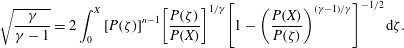
 $$\begin{eqnarray}\displaystyle & \displaystyle \sqrt{\frac{\unicode[STIX]{x1D6FE}}{\unicode[STIX]{x1D6FE}-1}}=2\int _{0}^{X}\left[\frac{P(\unicode[STIX]{x1D701})}{P(X)}\right]^{1/\unicode[STIX]{x1D6FE}}\left[1-\left(\frac{P(X)}{P(\unicode[STIX]{x1D701})}\right)^{(\unicode[STIX]{x1D6FE}-1)/\unicode[STIX]{x1D6FE}}\right]^{-1/2}\text{d}\unicode[STIX]{x1D701}. & \displaystyle\end{eqnarray}$$
Equations (2.20) and (2.21) slightly differ from the result obtained by Balakrishnan et al. (Reference Balakrishnan, Liñan and Williams1991), where an extra $(\unicode[STIX]{x1D701}/X)$
term appears as part of the integrand.
$(\unicode[STIX]{x1D701}/X)$
term appears as part of the integrand.
2.6 Integral formulation with pressure dependence
In practice, $U_{w}(\unicode[STIX]{x1D709})$
and
$U_{w}(\unicode[STIX]{x1D709})$
and $p(\unicode[STIX]{x1D709})$
may be linked according to Saint-Robert’s burning-rate law with constant
$p(\unicode[STIX]{x1D709})$
may be linked according to Saint-Robert’s burning-rate law with constant $K$
and
$K$
and $n$
,
$n$
,
 $$\begin{eqnarray}m_{w}=\unicode[STIX]{x1D70C}_{w}U_{w}=Kp^{n},\end{eqnarray}$$
where $m_{w}$
represents the mass flux at the wall. Then using the ideal gas law to eliminate the density, the injection velocity may be expressed as
$m_{w}$
represents the mass flux at the wall. Then using the ideal gas law to eliminate the density, the injection velocity may be expressed as
 $$\begin{eqnarray}U_{w}=\left(\frac{\unicode[STIX]{x1D6FE}-1}{\unicode[STIX]{x1D6FE}}\right)c_{p}\frac{T_{w}(\unicode[STIX]{x1D709})}{p(\unicode[STIX]{x1D709})}m_{w}(\unicode[STIX]{x1D709}).\end{eqnarray}$$
After substituting $U_{w}$
into (2.16), the dimensionless forms of
$U_{w}$
into (2.16), the dimensionless forms of $P(X)$
,
$P(X)$
, $X$
and
$X$
and $\unicode[STIX]{x1D701}$
may be updated viz.
$\unicode[STIX]{x1D701}$
may be updated viz.
 $$\begin{eqnarray}\displaystyle & \displaystyle P(X)=\frac{p(x)}{p_{0}}, & \displaystyle\end{eqnarray}$$
 $$\begin{eqnarray}\displaystyle & \displaystyle X=\sqrt{\frac{\unicode[STIX]{x1D6FE}-1}{\unicode[STIX]{x1D6FE}}}\frac{Kp_{0}^{n-1}}{2a}\int _{0}^{x}\sqrt{2c_{p}T_{w}(x^{\prime })}\,\text{d}x^{\prime }, & \displaystyle\end{eqnarray}$$
 $$\begin{eqnarray}\displaystyle & \displaystyle \unicode[STIX]{x1D701}=\sqrt{\frac{\unicode[STIX]{x1D6FE}-1}{\unicode[STIX]{x1D6FE}}}\frac{Kp_{0}^{n-1}}{2a}\int _{0}^{\unicode[STIX]{x1D709}}\sqrt{2c_{p}T_{w}(x^{\prime })}\,\text{d}x^{\prime }. & \displaystyle\end{eqnarray}$$
At length, equations (2.15) and (2.16) become
 $$\begin{eqnarray}\displaystyle & \displaystyle \left(\frac{r}{a}\right)^{2}=2\sqrt{\frac{\unicode[STIX]{x1D6FE}-1}{\unicode[STIX]{x1D6FE}}}\int _{0}^{\unicode[STIX]{x1D701}}[P(\unicode[STIX]{x1D701}^{\prime })]^{n-1}\left[\frac{P(\unicode[STIX]{x1D701}^{\prime })}{P(X)}\right]^{1/\unicode[STIX]{x1D6FE}}\left[1-\left(\frac{P(X)}{P(\unicode[STIX]{x1D701}^{\prime })}\right)^{(\unicode[STIX]{x1D6FE}-1)/\unicode[STIX]{x1D6FE}}\right]^{-1/2}\,\text{d}\unicode[STIX]{x1D701}^{\prime },\qquad & \displaystyle\end{eqnarray}$$
 $$\begin{eqnarray}\displaystyle & \displaystyle \sqrt{\frac{\unicode[STIX]{x1D6FE}}{\unicode[STIX]{x1D6FE}-1}}=2\int _{0}^{X}[P(\unicode[STIX]{x1D701})]^{n-1}\left[\frac{P(\unicode[STIX]{x1D701})}{P(X)}\right]^{1/\unicode[STIX]{x1D6FE}}\left[1-\left(\frac{P(X)}{P(\unicode[STIX]{x1D701})}\right)^{(\unicode[STIX]{x1D6FE}-1)/\unicode[STIX]{x1D6FE}}\right]^{-1/2}\,\text{d}\unicode[STIX]{x1D701}.\qquad & \displaystyle\end{eqnarray}$$
The procedure for solving this problem consists of integrating (2.28) to the extent of determining the pressure as a function of $x$
. Equation (2.27) can then be evaluated to deduce the radial coordinate in terms of
$x$
. Equation (2.27) can then be evaluated to deduce the radial coordinate in terms of $x$
and
$x$
and $\unicode[STIX]{x1D709}$
. With the pressure distribution at hand, the temperature may be obtained using the isentropic relation of (2.13). Lastly, the velocity may be extracted from the total temperature given by (2.12).
$\unicode[STIX]{x1D709}$
. With the pressure distribution at hand, the temperature may be obtained using the isentropic relation of (2.13). Lastly, the velocity may be extracted from the total temperature given by (2.12).
In the calculation of the Mach number, the compressible relation, $M=u/$ $\sqrt{(\unicode[STIX]{x1D6FE}-1)c_{p}T}$
, may be readily employed. In fact, the substitution of (2.12) into the Mach number relation leads to
$\sqrt{(\unicode[STIX]{x1D6FE}-1)c_{p}T}$
, may be readily employed. In fact, the substitution of (2.12) into the Mach number relation leads to
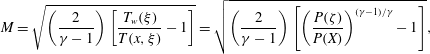 $$\begin{eqnarray}M=\sqrt{\left(\frac{2}{\unicode[STIX]{x1D6FE}-1}\right)\left[\frac{T_{w}(\unicode[STIX]{x1D709})}{T(x,\unicode[STIX]{x1D709})}-1\right]}=\sqrt{\left(\frac{2}{\unicode[STIX]{x1D6FE}-1}\right)\left[\left(\frac{P(\unicode[STIX]{x1D701})}{P(X)}\right)^{(\unicode[STIX]{x1D6FE}-1)/\unicode[STIX]{x1D6FE}}-1\right]},\end{eqnarray}$$
where the expression on the right-hand side may be obtained using the isentropic identity given by (2.13).
2.7 Numerical integration
In the numerical integration of (2.28), an inverse procedure is pursued. This is accomplished by switching to $P$
as the independent variable, and calculating
$P$
as the independent variable, and calculating $X$
in increments of
$X$
in increments of $\unicode[STIX]{x0394}P$
. The scheme begins at the headwall boundary where
$\unicode[STIX]{x0394}P$
. The scheme begins at the headwall boundary where $X=0$
at
$X=0$
at $P=1$
. The discretized pressure field can be expressed by
$P=1$
. The discretized pressure field can be expressed by $P_{i}=1-i\unicode[STIX]{x0394}P$
. Subsequently, one may solve for
$P_{i}=1-i\unicode[STIX]{x0394}P$
. Subsequently, one may solve for $X_{i}$
at every step until choking conditions, which occur when
$X_{i}$
at every step until choking conditions, which occur when $\text{d}P/\text{d}X\rightarrow \infty$
. Bearing these constraints in mind, a variable transformation in (2.28) results in
$\text{d}P/\text{d}X\rightarrow \infty$
. Bearing these constraints in mind, a variable transformation in (2.28) results in
 $$\begin{eqnarray}2\sqrt{\frac{\unicode[STIX]{x1D6FE}-1}{\unicode[STIX]{x1D6FE}}}\!\int _{P}^{1}(P^{\prime })^{n-1}\left(\frac{P^{\prime }}{P}\right)^{1/\unicode[STIX]{x1D6FE}}\left[1-\left(\frac{P}{P^{\prime }}\right)^{(\unicode[STIX]{x1D6FE}-1)/\unicode[STIX]{x1D6FE}}\right]^{-1/2}\!\left[-\frac{\text{d}X(P^{\prime })}{\text{d}P^{\prime }}\right]\text{d}P^{\prime }=\int _{P}^{1}f(P^{\prime })\,\text{d}P^{\prime }=1.\end{eqnarray}$$
Toovercomethesingularities that appear at the boundaries,this integral is subsequently split into three parts, specifically,
 $$\begin{eqnarray}\underbrace{\int _{P_{i}}^{P_{i+1}}f(P^{\prime })\,\text{d}P^{\prime }}_{1}+\underbrace{\int _{P_{i+1}}^{1-\unicode[STIX]{x0394}P}f(P^{\prime })\,\text{d}P^{\prime }}_{2}+\underbrace{\int _{1-\unicode[STIX]{x0394}P}^{1}f(P^{\prime })\,\text{d}P^{\prime }}_{3}=1.\end{eqnarray}$$
In the region near $P=P_{i}$
, the first integrand may be approximated such that an expression may be retrieved in a form that is straightforward to evaluate for an arbitrary pressure exponent
$P=P_{i}$
, the first integrand may be approximated such that an expression may be retrieved in a form that is straightforward to evaluate for an arbitrary pressure exponent $n$
. We get
$n$
. We get
 $$\begin{eqnarray}\int _{P_{i}}^{P_{i+1}}f(P^{\prime })\,\text{d}P^{\prime }\approx 2\int _{P_{i}}^{P_{i+1}}(P^{\prime })^{n-1}\left(\frac{P^{\prime }-P_{i}}{P^{\prime }}\right)^{-1/2}\left(-\frac{\text{d}X}{\text{d}P}\right)_{i}\text{d}P^{\prime }.\end{eqnarray}$$
The second integral may be computed, for example, using the trapezoidal rule. This involves finite step discretization,
 $$\begin{eqnarray}\int _{P_{i+1}}^{1-\unicode[STIX]{x0394}P}f(P^{\prime })\,\text{d}P^{\prime }\approx \unicode[STIX]{x0394}P\left(\frac{f_{1}+f_{i+1}}{2}+\mathop{\sum }_{k=2}^{i+2}f_{k}\right),\end{eqnarray}$$
where
 $$\begin{eqnarray}f_{k}=2\sqrt{\frac{\unicode[STIX]{x1D6FE}-1}{\unicode[STIX]{x1D6FE}}}[P_{k}]^{n-1}\left[\frac{P_{k}}{P_{i}}\right]^{1/\unicode[STIX]{x1D6FE}}\left[1-\left(\frac{P_{i}}{P_{k}}\right)^{(\unicode[STIX]{x1D6FE}-1)/\unicode[STIX]{x1D6FE}}\right]^{-1/2}\left(-\frac{\text{d}X}{\text{d}P}\right)_{k}.\end{eqnarray}$$
In the third integral, where $X$
is small,
$X$
is small, $P(X)$
may be expanded using a polynomial of the form
$P(X)$
may be expanded using a polynomial of the form
 $$\begin{eqnarray}P(X)=1-\unicode[STIX]{x1D6FC}X^{2}+\cdots .\end{eqnarray}$$
By inserting (2.35) into the integral and assuming $\unicode[STIX]{x1D6FC}\unicode[STIX]{x1D701}^{2}\ll 1$
, we are left with
$\unicode[STIX]{x1D6FC}\unicode[STIX]{x1D701}^{2}\ll 1$
, we are left with
 $$\begin{eqnarray}\int _{1-\unicode[STIX]{x0394}P}^{1}f(P^{\prime })\,\text{d}P^{\prime }\approx 2\sqrt{\frac{\unicode[STIX]{x1D6FE}-1}{\unicode[STIX]{x1D6FE}}}(P_{i})^{-1/\unicode[STIX]{x1D6FE}}\left[1-(P_{i})^{(\unicode[STIX]{x1D6FE}-1)/\unicode[STIX]{x1D6FE}}\right]^{-1/2}\sqrt{\frac{\unicode[STIX]{x0394}P}{\unicode[STIX]{x1D6FC}}}.\end{eqnarray}$$
To evaluate (2.36), $\unicode[STIX]{x1D6FC}$
must be determined beforehand. We accomplish this by substituting (2.35) into (2.28) and returning
$\unicode[STIX]{x1D6FC}$
must be determined beforehand. We accomplish this by substituting (2.35) into (2.28) and returning
 $$\begin{eqnarray}\frac{2}{\sqrt{\unicode[STIX]{x1D6FC}}}\int _{0}^{X}\frac{1}{\sqrt{X^{2}-\unicode[STIX]{x1D701}^{2}}}\,\text{d}\unicode[STIX]{x1D701}=1.\end{eqnarray}$$
We thus deduce that a value of $\unicode[STIX]{x1D6FC}=\unicode[STIX]{x03C0}^{2}$
will be needed to satisfy (2.37).
$\unicode[STIX]{x1D6FC}=\unicode[STIX]{x03C0}^{2}$
will be needed to satisfy (2.37).
Equation (2.31) is now linear in $X_{i}$
. Starting with
$X_{i}$
. Starting with $X=0$
at
$X=0$
at $P=1$
, one may solve for
$P=1$
, one may solve for $X_{i}$
at every step until choking conditions are attained, at which point the average Mach number reaches unity. In the cases described hereafter, we take
$X_{i}$
at every step until choking conditions are attained, at which point the average Mach number reaches unity. In the cases described hereafter, we take $\unicode[STIX]{x0394}P$
to be
$\unicode[STIX]{x0394}P$
to be $5\times 10^{-4}$
. With the pressure distribution fully determined, it may be substituted into (2.27) and integrated numerically. This step returns the corresponding radius, which is needed for a complete description of the streamlines. Equations (2.12) and (2.13) may then be utilized to extract the temperature and velocity. The resulting process is illustrated in figure 2, where a procedural flowchart is furnished.
$5\times 10^{-4}$
. With the pressure distribution fully determined, it may be substituted into (2.27) and integrated numerically. This step returns the corresponding radius, which is needed for a complete description of the streamlines. Equations (2.12) and (2.13) may then be utilized to extract the temperature and velocity. The resulting process is illustrated in figure 2, where a procedural flowchart is furnished.
Flowchart depicting the main steps of the numerical procedure needed to extract the velocity from the integral formulation of the pressure.

3 Results and discussion
3.1 On the pressure and temperature variations
After solving (2.30) in decrements of $\unicode[STIX]{x0394}P$
, the pressure may be reproduced as a function of
$\unicode[STIX]{x0394}P$
, the pressure may be reproduced as a function of $x$
. Assuming a constant temperature along the sidewall, the resulting solutions for
$x$
. Assuming a constant temperature along the sidewall, the resulting solutions for $P$
and
$P$
and $T$
are showcased in figure 3 for
$T$
are showcased in figure 3 for $n=0$
and
$n=0$
and $n=1$
. Also shown on the graphs are the analytical predictions based on the one-dimensional theory of Gany & Aharon (Reference Gany and Aharon1999), and the two-dimensional analysis of Majdalani (Reference Majdalani2007).
$n=1$
. Also shown on the graphs are the analytical predictions based on the one-dimensional theory of Gany & Aharon (Reference Gany and Aharon1999), and the two-dimensional analysis of Majdalani (Reference Majdalani2007).
Based on figure 3, a qualitative agreement may be seen to occur between the present, semi-analytical formulation, and Majdalani’s closed-form solution. The same may be said concerning the one-dimensional solution of Gany & Aharon (Reference Gany and Aharon1999), despite its entirely dissimilar form. The small differences separating these estimates may be attributed to their underlying assumptions. On the one hand, the instantaneous burning rate of the one-dimensional solution is taken to be uniform along the grain, thus leading to a constant mass flux at the simulated propellant surface. A corresponding relation may be reproduced in the present solution by setting $n=0$
, as reflected in the improved agreement with one-dimensional theory (see figure 3
a,b). In summary the one-dimensional model predicts
$n=0$
, as reflected in the improved agreement with one-dimensional theory (see figure 3
a,b). In summary the one-dimensional model predicts
 $$\begin{eqnarray}\displaystyle & \displaystyle \left.\begin{array}{@{}c@{}}\displaystyle M_{1D}=\sqrt{\frac{1-\sqrt{1-\unicode[STIX]{x1D712}^{2}}}{1+\unicode[STIX]{x1D6FE}\sqrt{1-\unicode[STIX]{x1D712}^{2}}}};\quad \unicode[STIX]{x1D712}\equiv \frac{x}{L_{s}};\quad P_{1D}=\frac{1+\unicode[STIX]{x1D6FE}\sqrt{1-\unicode[STIX]{x1D712}^{2}}}{1+\unicode[STIX]{x1D6FE}},\\ \displaystyle T_{1D}=\left(\frac{1+\unicode[STIX]{x1D6FE}\sqrt{1-\unicode[STIX]{x1D712}^{2}}}{1+\unicode[STIX]{x1D6FE}}\right)^{1-1/\unicode[STIX]{x1D6FE}}.\end{array}\right\} & \displaystyle\end{eqnarray}$$
Comparison between the present semi-analytical formulation and both one- and two-dimensional solutions by Gany & Aharon (Reference Gany and Aharon1999) and Majdalani (Reference Majdalani2007). Results are provided for the (a,c) pressure and (b,d) temperature distributions using $\unicode[STIX]{x1D6FE}=1.4$
,
$\unicode[STIX]{x1D6FE}=1.4$
, $M_{w}=0.05$
, and either
$M_{w}=0.05$
, and either $n=0$
(constant mass flux), or
$n=0$
(constant mass flux), or $n=1$
(constant wall injection speed). Also shown in (c,d) is the
$n=1$
(constant wall injection speed). Also shown in (c,d) is the $n=0.67$
case corresponding to solid propellant burning.
$n=0.67$
case corresponding to solid propellant burning.

On the other hand, the uniform sidewall injection velocity of the two-dimensional axisymmetric solution of Majdalani (Reference Majdalani2007) corresponds to the $n=1$
case presented here. This may also explain the improved agreement with two-dimensional theory in figure 3(c,d). In the interest of clarity, the two-dimensional solution obtained by Majdalani (Reference Majdalani2007) is reproduced in appendix A.
$n=1$
case presented here. This may also explain the improved agreement with two-dimensional theory in figure 3(c,d). In the interest of clarity, the two-dimensional solution obtained by Majdalani (Reference Majdalani2007) is reproduced in appendix A.
In figure 3(a,b), the reason for the slight discrepancy at $n=0$
between our predictions and those of the one-dimensional analytical model may be attributed to two-dimensional effects. As for the
$n=0$
between our predictions and those of the one-dimensional analytical model may be attributed to two-dimensional effects. As for the $n=1$
case, the present model in figure 3(c,d) appears to be in relatively good agreement with the two-dimensional approximation everywhere except in the vicinity of the choke point, where the difference reaches approximately 2 % at
$n=1$
case, the present model in figure 3(c,d) appears to be in relatively good agreement with the two-dimensional approximation everywhere except in the vicinity of the choke point, where the difference reaches approximately 2 % at $x/L_{s}=0.9$
. Specifically, the tailing ends of the numerical curves in figure 3(c,d) undergo an abrupt steepening process as
$x/L_{s}=0.9$
. Specifically, the tailing ends of the numerical curves in figure 3(c,d) undergo an abrupt steepening process as $x\rightarrow L_{s}$
, thus leading to a minor departure from the two-dimensional formulation. Two possible explanations may be offered in this respect. The first may be attributed to the linear approximation affecting pressure integration in (2.32), especially that these approximations can deteriorate near the choke point. The second source of disparity may be connected with the accuracy of the Rayleigh–Janzen expansion used by Majdalani (Reference Majdalani2007) in the vicinity of
$x\rightarrow L_{s}$
, thus leading to a minor departure from the two-dimensional formulation. Two possible explanations may be offered in this respect. The first may be attributed to the linear approximation affecting pressure integration in (2.32), especially that these approximations can deteriorate near the choke point. The second source of disparity may be connected with the accuracy of the Rayleigh–Janzen expansion used by Majdalani (Reference Majdalani2007) in the vicinity of $x=L_{s}$
. However, as shown by Tollmien (Reference Tollmien1941) and further confirmed by Kaplan (Reference Kaplan1946), the Rayleigh–Janzen paradigm continues to hold past sonic conditions. As for the
$x=L_{s}$
. However, as shown by Tollmien (Reference Tollmien1941) and further confirmed by Kaplan (Reference Kaplan1946), the Rayleigh–Janzen paradigm continues to hold past sonic conditions. As for the $n=0.67$
case, which has been attributed to solid propellant regression rate behaviour, the corresponding chained lines in figure 3(c,d) reflect a slight increase in the local pressure and temperature along the length of the chamber relative to the constant
$n=0.67$
case, which has been attributed to solid propellant regression rate behaviour, the corresponding chained lines in figure 3(c,d) reflect a slight increase in the local pressure and temperature along the length of the chamber relative to the constant $U_{w}$
model.
$U_{w}$
model.
Another factor that may have a bearing on the observed differences may be connected to the underlying thermodynamic conditions adopted in these models. For example, by holding entropy constant along streamlines, the present solution proves to be isentropic, whereas Majdalani’s formulation, which assumes constant entropy along the injecting wall, leads to a strictly homentropic model. Taken over the entire fluid domain, Majdalani (Reference Majdalani2007) assumes
 $$\begin{eqnarray}T/T_{0}=(p/p_{0})^{(\unicode[STIX]{x1D6FE}-1)/\unicode[STIX]{x1D6FE}},\end{eqnarray}$$
with the corresponding entropy change amounting to:
 $$\begin{eqnarray}s-s_{0}=c_{p}\ln (T/T_{0})-R\ln (p/p_{0}),\end{eqnarray}$$
where the subscript 0 denotes a reference point. Clearly, when (3.2) is inserted into (3.3), it leads to the vanishing of the entropy change throughout the chamber. However, in the present formulation, we recall that (2.10) reduces the entropy changes along a streamline, and would thus account for entropy changes as the flow progresses downstream. In reality, as the critical distance is approached, both turbulence and viscous effects become significant, and these may render any reversible flow assumption invalid. In this event, the homentropic approximation, which prevents entropy from varying in the streamwise direction, is likely to become less accurate than the isentropic formulation.
Before leaving this section, it may be interesting to note that the four parts of figure 3 are obtained using a single value of the wall Mach number, namely, of 0.05. Nonetheless, these plots remain characteristic of the solution at other wall Mach numbers. This may be attributed to the results being displayed as function of the geometric similarity coordinate, $\unicode[STIX]{x1D712}\equiv x/L_{s}$
. As one may surmise from (A 1) to (A 4), the similarity with respect to
$\unicode[STIX]{x1D712}\equiv x/L_{s}$
. As one may surmise from (A 1) to (A 4), the similarity with respect to $\unicode[STIX]{x1D712}$
leads to a formulation that is virtually independent of
$\unicode[STIX]{x1D712}$
leads to a formulation that is virtually independent of $M_{w}$
. Another interesting feature may be associated with the sonic to headwall pressure ratio, as it may be evaluated to be 0.3361 in the present formulation, thus lower than the pressure ratio obtained from one-dimensional and two-dimensional theories which, for
$M_{w}$
. Another interesting feature may be associated with the sonic to headwall pressure ratio, as it may be evaluated to be 0.3361 in the present formulation, thus lower than the pressure ratio obtained from one-dimensional and two-dimensional theories which, for $\unicode[STIX]{x1D6FE}=1.4$
, yield
$\unicode[STIX]{x1D6FE}=1.4$
, yield $(1+\unicode[STIX]{x1D6FE})^{-1}\approx 0.4167$
and 0.5013, respectively.
$(1+\unicode[STIX]{x1D6FE})^{-1}\approx 0.4167$
and 0.5013, respectively.
3.2 On the local Mach number and critical length calculations
With the present study being axisymmetric, the calculation of the critical length, which is otherwise straightforward to define in one-dimensional space, deserves special attention. In the classic sense, $L_{s}$
denotes the distance from the headwall to the point along the axis where the centreline speed reaches the velocity of sound (Majdalani Reference Majdalani2007). At this location, however, the bulk motion of the gases remains subsonic everywhere except at
$L_{s}$
denotes the distance from the headwall to the point along the axis where the centreline speed reaches the velocity of sound (Majdalani Reference Majdalani2007). At this location, however, the bulk motion of the gases remains subsonic everywhere except at $r=0$
. Evidently, a new definition of the critical length is warranted, specifically one that considers the flow to be choked only when the local area-averaged Mach number,
$r=0$
. Evidently, a new definition of the critical length is warranted, specifically one that considers the flow to be choked only when the local area-averaged Mach number, $\overline{M}$
, would have reached unity. To this end, an area-averaged critical length,
$\overline{M}$
, would have reached unity. To this end, an area-averaged critical length, $\overline{L}_{s}$
, may be introduced, where
$\overline{L}_{s}$
, may be introduced, where $\overline{L}_{s}>L_{s}$
. In fact, typical values of
$\overline{L}_{s}>L_{s}$
. In fact, typical values of $\overline{L}_{s}$
seem to vary between 1.1 and
$\overline{L}_{s}$
seem to vary between 1.1 and $1.2L_{s}$
, depending on the model and gas property
$1.2L_{s}$
, depending on the model and gas property $\unicode[STIX]{x1D6FE}$
.
$\unicode[STIX]{x1D6FE}$
.
Using $\overline{L}_{s}$
as a reference length scale in the streamwise direction, a comparison of the centreline Mach number,
$\overline{L}_{s}$
as a reference length scale in the streamwise direction, a comparison of the centreline Mach number, $M_{c}$
, is provided in figure 4(a,b) for
$M_{c}$
, is provided in figure 4(a,b) for $n=0$
and
$n=0$
and $n=1$
, respectively. In both parts of the graph, the two-dimensional analytical model is seen to outperform the one-dimensional solution, although better agreement with the integral representation appears in figure 4(b). This behaviour may have been anticipated because the axisymmetric analytic model is derived under the
$n=1$
, respectively. In both parts of the graph, the two-dimensional analytical model is seen to outperform the one-dimensional solution, although better agreement with the integral representation appears in figure 4(b). This behaviour may have been anticipated because the axisymmetric analytic model is derived under the $n=1$
assumption. Another point of disparity may be associated with the centreline Mach numbers exceeding unity at
$n=1$
assumption. Another point of disparity may be associated with the centreline Mach numbers exceeding unity at $x=\overline{L}_{s}$
. Conversely, the one-dimensional Mach number, in which area-averaging is intrinsic, is seen to reach sonic conditions at
$x=\overline{L}_{s}$
. Conversely, the one-dimensional Mach number, in which area-averaging is intrinsic, is seen to reach sonic conditions at $x=\overline{L}_{s}.$
As shown in figure 4(c,d), the analytical area-averaged Mach number and, in principle, our numerically area-averaged solution, exhibit steeper curvatures that closely follow the dotted, one-dimensional prediction.
$x=\overline{L}_{s}.$
As shown in figure 4(c,d), the analytical area-averaged Mach number and, in principle, our numerically area-averaged solution, exhibit steeper curvatures that closely follow the dotted, one-dimensional prediction.
Evolution of centreline Mach numbers along with available one- and two-dimensional solutions for (a) $n=0$
and (b)
$n=0$
and (b) $n=1$
. The same is repeated using the area-averaged Mach number for (c)
$n=1$
. The same is repeated using the area-averaged Mach number for (c) $n=0$
and (d)
$n=0$
and (d) $n=1$
. Here
$n=1$
. Here $\unicode[STIX]{x1D6FE}=1.4$
and
$\unicode[STIX]{x1D6FE}=1.4$
and $M_{w}=0.05$
.
$M_{w}=0.05$
.

It may be instructive to add that, based on (2.29), the Mach number may be calculated over the entire chamber. However, owing to the variables being expressed in terms of the axial location and the streamfunction tip $\unicode[STIX]{x1D709}$
, a transformation is required to convert
$\unicode[STIX]{x1D709}$
, a transformation is required to convert $\unicode[STIX]{x1D709}$
back to the radial coordinate by way of (2.27). The resulting operation leads to a non-uniform mesh that requires careful treatment and reverse engineering. After some effort, the contour plots of the numerically extracted local Mach numbers are displayed in figure 5 using solid lines, where the shape of the
$\unicode[STIX]{x1D709}$
back to the radial coordinate by way of (2.27). The resulting operation leads to a non-uniform mesh that requires careful treatment and reverse engineering. After some effort, the contour plots of the numerically extracted local Mach numbers are displayed in figure 5 using solid lines, where the shape of the $M=1$
curve is clearly delineated. Here the axisymmetric analytical predictions of the iso-Mach number lines are presented side by side using broken lines.
$M=1$
curve is clearly delineated. Here the axisymmetric analytical predictions of the iso-Mach number lines are presented side by side using broken lines.
Despite the slight dissimilarity in their contour curvatures near choking (upper rightmost corner), the two models seem to display visible agreement in their Mach number predictions everywhere else. Clearly, the traditional concept of a choke point proves to be limited, as the iso-Mach number contours consist of lines of revolution about the chamber axis. At the outset, the actual locus of sonic velocities forms a curved surface that can be captured either numerically or analytically for $M=1$
. In the present configuration, such a condition can only be realized along a two-dimensional axisymmetric surface instead of a local point.
$M=1$
. In the present configuration, such a condition can only be realized along a two-dimensional axisymmetric surface instead of a local point.
Before leaving this section, it may be useful to note that figures 4 and 5 retain a rather universal character; being plotted versus $x/L_{s}$
, these graphs will not change if a different wall Mach number is used to reproduce them. This too may be attributed to the geometric self-similarity with respect to
$x/L_{s}$
, these graphs will not change if a different wall Mach number is used to reproduce them. This too may be attributed to the geometric self-similarity with respect to $\unicode[STIX]{x1D712}$
, which is consistent with (A 1)–(A 4).
$\unicode[STIX]{x1D712}$
, which is consistent with (A 1)–(A 4).
Local Mach number contours for constant wall injection speed using the present integral formulation (——) as well as the axisymmetric analytical approximation (– – –) obtained by Majdalani (Reference Majdalani2007). Here $n=1$
,
$n=1$
, $\unicode[STIX]{x1D6FE}=1.4$
and
$\unicode[STIX]{x1D6FE}=1.4$
and $M_{w}=0.01$
.
$M_{w}=0.01$
.

3.3 Compressible streamlines
Having completed our description of the Mach number variation, characteristic streamlines are displayed in figure 6 based on the numerical integration of (2.27). This is carried out by first specifying a value of $\unicode[STIX]{x1D709}$
, and then integrating at discrete locations of
$\unicode[STIX]{x1D709}$
, and then integrating at discrete locations of $x$
until the centreline Mach number has reached unity. The corresponding point marks the critical distance to the sonic point, which enables us to calculate
$x$
until the centreline Mach number has reached unity. The corresponding point marks the critical distance to the sonic point, which enables us to calculate $L_{s}$
for each of the test cases at hand. The procedure also enables us to collect the family of coordinates at a fixed value of
$L_{s}$
for each of the test cases at hand. The procedure also enables us to collect the family of coordinates at a fixed value of $\unicode[STIX]{x1D709}$
, thus leading to an assortment of points that constitute a streamline. By comparing the results in figure 6 at two wall Mach numbers of (a) 0.01 and (b) 0.005, it is clear that compressibility becomes more pronounced when the mean-flow velocity is increased (for
$\unicode[STIX]{x1D709}$
, thus leading to an assortment of points that constitute a streamline. By comparing the results in figure 6 at two wall Mach numbers of (a) 0.01 and (b) 0.005, it is clear that compressibility becomes more pronounced when the mean-flow velocity is increased (for $\unicode[STIX]{x1D6FE}=1.4$
). This is reflected in the faster flow turning that occurs at higher injection Mach numbers, specifically in figure 6(a), where
$\unicode[STIX]{x1D6FE}=1.4$
). This is reflected in the faster flow turning that occurs at higher injection Mach numbers, specifically in figure 6(a), where $L_{s}\cong 24.44$
, than in figure 6(b), where
$L_{s}\cong 24.44$
, than in figure 6(b), where $L_{s}\cong 48.87$
. However, by replotting these two cases in terms of
$L_{s}\cong 48.87$
. However, by replotting these two cases in terms of $x/L_{s}$
, the ensuing graphs become identical. This visual artefact is caused by the strong similarity of the flow motion with respect to
$x/L_{s}$
, the ensuing graphs become identical. This visual artefact is caused by the strong similarity of the flow motion with respect to $\unicode[STIX]{x1D712}$
.
$\unicode[STIX]{x1D712}$
.
Numerical streamlines for (a) $M_{w}=0.01$
and (b)
$M_{w}=0.01$
and (b) $M_{w}=0.005$
compared to the incompressible solution by Culick (Reference Culick1966). Here
$M_{w}=0.005$
compared to the incompressible solution by Culick (Reference Culick1966). Here $\unicode[STIX]{x1D6FE}=1.4$
.
$\unicode[STIX]{x1D6FE}=1.4$
.

3.4 Axial and radial velocities
As alluded to in the flowchart of figure 2, the last procedural step consists of extracting the axial velocity from (2.12). The outcome is featured in figure 7 where $u$
is depicted at evenly spaced intervals of
$u$
is depicted at evenly spaced intervals of $x/\overline{L}_{s}=0.2,0.4,\ldots ,1$
, and for injection wall Mach numbers of (a) 0.01 and (b) 0.005. Graphically, it may be interesting to observe the strong similarity in the evolution of the velocity profile with respect to
$x/\overline{L}_{s}=0.2,0.4,\ldots ,1$
, and for injection wall Mach numbers of (a) 0.01 and (b) 0.005. Graphically, it may be interesting to observe the strong similarity in the evolution of the velocity profile with respect to $\unicode[STIX]{x1D712}$
. Also featured on the graph is the two-dimensional analytical solution by Majdalani (Reference Majdalani2007). Unsurprisingly, these results compare quite favourably to the numerical simulations and laboratory measurements reported by Traineau et al. (Reference Traineau, Hervat and Kuentzmann1986), Balakrishnan et al. (Reference Balakrishnan, Liñan and Williams1992), and Apte & Yang (Reference Apte and Yang2001). By comparison to Taylor–Culick’s incompressible mean-flow solution, it may be seen that the axial velocity develops into a blunter, top-hat profile as
$\unicode[STIX]{x1D712}$
. Also featured on the graph is the two-dimensional analytical solution by Majdalani (Reference Majdalani2007). Unsurprisingly, these results compare quite favourably to the numerical simulations and laboratory measurements reported by Traineau et al. (Reference Traineau, Hervat and Kuentzmann1986), Balakrishnan et al. (Reference Balakrishnan, Liñan and Williams1992), and Apte & Yang (Reference Apte and Yang2001). By comparison to Taylor–Culick’s incompressible mean-flow solution, it may be seen that the axial velocity develops into a blunter, top-hat profile as $x\rightarrow \overline{L}_{s}$
. The steepening of the solution into a fuller, turbulent-like, slug motion is consistent with both theoretical and experimental predictions. It is accompanied by progressively sharper wall gradients that significantly alter the mean-flow character.
$x\rightarrow \overline{L}_{s}$
. The steepening of the solution into a fuller, turbulent-like, slug motion is consistent with both theoretical and experimental predictions. It is accompanied by progressively sharper wall gradients that significantly alter the mean-flow character.
Spatial evolution of the axial velocity for (a) $M_{w}=0.01$
and (b)
$M_{w}=0.01$
and (b) $M_{w}=0.005$
at
$M_{w}=0.005$
at $x/\overline{L}_{s}=0.2$
, 0.4, 0.6, 0.8, and 1. Results are compared to the compressible solution by Majdalani (Reference Majdalani2007). Here
$x/\overline{L}_{s}=0.2$
, 0.4, 0.6, 0.8, and 1. Results are compared to the compressible solution by Majdalani (Reference Majdalani2007). Here $\unicode[STIX]{x1D6FE}=1.4$
.
$\unicode[STIX]{x1D6FE}=1.4$
.

With the axial velocity in hand, one can deduce the radial velocity evolution from the continuity equation. In this manner, a numerical approximation of $v$
may be retrieved and presented in figure 8(a), at multiple locations in the chamber; this is mainly done to aid in visualizing the actual development of the profile as the flow advances downstream. Here too, the radial velocity approximation by Majdalani (Reference Majdalani2007) is depicted in figure 8(b) to showcase the consistent agreement between the two models.
$v$
may be retrieved and presented in figure 8(a), at multiple locations in the chamber; this is mainly done to aid in visualizing the actual development of the profile as the flow advances downstream. Here too, the radial velocity approximation by Majdalani (Reference Majdalani2007) is depicted in figure 8(b) to showcase the consistent agreement between the two models.
Spatial evolution of the radial velocity for $M_{w}=0.01$
at
$M_{w}=0.01$
at $x/\overline{L}_{s}=0.2$
, 0.4, and 0.6 according to (a) the present solution and (b) the compressible model by Majdalani (Reference Majdalani2007).
$x/\overline{L}_{s}=0.2$
, 0.4, and 0.6 according to (a) the present solution and (b) the compressible model by Majdalani (Reference Majdalani2007).

3.5 Computational verification
The present model may be compared to numerical simulations using a second-order finite volume solver and two turbulent models, namely, the $k$
–
$k$
– $\unicode[STIX]{x1D714}$
and the Spalart–Allmaras relations, as well as a strictly inviscid solver. Based on (A 5), we estimate that an aspect ratio of 13 will be sufficient to induce sonic conditions, and proceed to define a porous tube of 1 m radius and 13 m length. Then, using air as a working fluid with a density of
$\unicode[STIX]{x1D714}$
and the Spalart–Allmaras relations, as well as a strictly inviscid solver. Based on (A 5), we estimate that an aspect ratio of 13 will be sufficient to induce sonic conditions, and proceed to define a porous tube of 1 m radius and 13 m length. Then, using air as a working fluid with a density of $1.18~\text{kg}~\text{m}^{-3}$
and a wall Mach number of 0.02, we impose a
$1.18~\text{kg}~\text{m}^{-3}$
and a wall Mach number of 0.02, we impose a $6.86~\text{m}~\text{s}^{-1}$
velocity inlet condition at the sidewall along with a static pressure of 101 720 Pa. Subsequently, the domain is discretized using 800 and 100 nodes in the axial and radial directions, respectively. We also use a Courant number of 70 and a relaxation factor of 0.5 until our convergence criterion of
$6.86~\text{m}~\text{s}^{-1}$
velocity inlet condition at the sidewall along with a static pressure of 101 720 Pa. Subsequently, the domain is discretized using 800 and 100 nodes in the axial and radial directions, respectively. We also use a Courant number of 70 and a relaxation factor of 0.5 until our convergence criterion of $10^{-7}$
is secured in the continuity, momentum, ideal gas, and energy equations.
$10^{-7}$
is secured in the continuity, momentum, ideal gas, and energy equations.
Comparison of the present solution to computational predictions from two turbulent models and a strictly inviscid compressible solver for (a) the pressure distribution, (b) the streamwise velocity at the critical length, (c) the temperature distribution, and (d) the centreline Mach number. Here $\unicode[STIX]{x1D6FE}=1.4$
,
$\unicode[STIX]{x1D6FE}=1.4$
, $L=13$
, and
$L=13$
, and $M_{w}=0.02$
.
$M_{w}=0.02$
.

After some post-processing, figure 9(a) is used to display the pressure distribution along the centreline, as done previously by Majdalani (Reference Majdalani2007). Although numerical simulations do not perfectly coincide with the theoretical models, the consistency in the sloping curvature of the various pressure profiles tends to confirm the effectiveness of the methods employed. This is especially true in the inviscid computation, which closely mimics the axial distribution of the present formulation, followed by the $k$
–
$k$
– $\unicode[STIX]{x1D714}$
and the Spalart–Allmaras simulations. The differences observed may be partly attributed to viscosity and turbulence effects, which are accounted for in the turbulent computations but not in the theoretical solutions. For instance, when viscosity is recognized as a damping agent, its presence may be seen to reduce the transfer of thermal to kinetic energy, and this deficiency leads to an increase in the chamber pressure everywhere except in the vicinity of the choking area. Also shown in figure 9(b) are comparisons of the streamwise velocity profiles, which are evaluated at the critical distance, where disparities between various models are most appreciable. Here the velocities are normalized with respect to the centreline speed in order to more effectively showcase the blunting character induced in the profile as a result of fluid dilatation. Interestingly, the centreline velocities predicted by the three computational models fall within a few percent of theoretical approximations. In this case, the Spalart–Allmaras model seems to outperform the
$\unicode[STIX]{x1D714}$
and the Spalart–Allmaras simulations. The differences observed may be partly attributed to viscosity and turbulence effects, which are accounted for in the turbulent computations but not in the theoretical solutions. For instance, when viscosity is recognized as a damping agent, its presence may be seen to reduce the transfer of thermal to kinetic energy, and this deficiency leads to an increase in the chamber pressure everywhere except in the vicinity of the choking area. Also shown in figure 9(b) are comparisons of the streamwise velocity profiles, which are evaluated at the critical distance, where disparities between various models are most appreciable. Here the velocities are normalized with respect to the centreline speed in order to more effectively showcase the blunting character induced in the profile as a result of fluid dilatation. Interestingly, the centreline velocities predicted by the three computational models fall within a few percent of theoretical approximations. In this case, the Spalart–Allmaras model seems to outperform the $k$
–
$k$
– $\unicode[STIX]{x1D714}$
simulation in matching the radial steepening of the axial flow profile in the mid-annular region between the centreline and the wall. The inviscid simulation, however, remains close to the integral formulation over the majority of the chamber radius, although its accuracy is occasionally matched near the wall by the
$\unicode[STIX]{x1D714}$
simulation in matching the radial steepening of the axial flow profile in the mid-annular region between the centreline and the wall. The inviscid simulation, however, remains close to the integral formulation over the majority of the chamber radius, although its accuracy is occasionally matched near the wall by the $k$
–
$k$
– $\unicode[STIX]{x1D714}$
computation.
$\unicode[STIX]{x1D714}$
computation.
Similar trends are captured in figures 9(c) and 9(d), where a strong agreement may be noted between the present approximation for the temperature and centreline Mach numbers, and simulations based on both inviscid and $k$
–
$k$
– $\unicode[STIX]{x1D714}$
models. In fact, the
$\unicode[STIX]{x1D714}$
models. In fact, the $k$
–
$k$
– $\unicode[STIX]{x1D714}$
predictions for the pressure and temperature seem to mirror those of the inviscid solver along the length of the chamber. In both figures 9(c) and 9(d), the agreement with the inviscid solver is most appreciable in the streamwise direction up to approximately 70 % and 80 % of the sonic length, respectively. In the remaining section of the chamber, the
$\unicode[STIX]{x1D714}$
predictions for the pressure and temperature seem to mirror those of the inviscid solver along the length of the chamber. In both figures 9(c) and 9(d), the agreement with the inviscid solver is most appreciable in the streamwise direction up to approximately 70 % and 80 % of the sonic length, respectively. In the remaining section of the chamber, the $k$
–
$k$
– $\unicode[STIX]{x1D714}$
simulations appear to be nearer to the integral model, although their deviations remain on the same order as that of the inviscid solver.
$\unicode[STIX]{x1D714}$
simulations appear to be nearer to the integral model, although their deviations remain on the same order as that of the inviscid solver.
Relative (a,c) and absolute deviations (b,d) between the present solution and the inviscid compressible solver (——) as well as the $k$
–
$k$
– $\unicode[STIX]{x1D714}$
(– – –) and the Spalart–Allmaras simulations (— ⋅ —) for (a) the pressure, (b) the streamwise velocity at the critical length, (c) the temperature, and (d) the centreline Mach number. Here
$\unicode[STIX]{x1D714}$
(– – –) and the Spalart–Allmaras simulations (— ⋅ —) for (a) the pressure, (b) the streamwise velocity at the critical length, (c) the temperature, and (d) the centreline Mach number. Here $\unicode[STIX]{x1D6FE}=1.4$
,
$\unicode[STIX]{x1D6FE}=1.4$
, $L=13$
, and
$L=13$
, and $M_{w}=0.02$
.
$M_{w}=0.02$
.

To better quantify these differences, a plot of each model’s deviation relative to the integral formulation is provided in figure 10. Consistently with the previous discussion, it may be seen in figure 10(a) that the relative deviation of the pressure acquired by the inviscid solver remains lower than its $k$
–
$k$
– $\unicode[STIX]{x1D714}$
and Spalart–Allmaras counterparts for
$\unicode[STIX]{x1D714}$
and Spalart–Allmaras counterparts for $0\leqslant x\leqslant \bar{L}_{s}$
. The same statement would have been applicable to figures 10(c) and 10(d) were it not for a small segment, not exceeding 20 %–30 % of the chamber length, where the
$0\leqslant x\leqslant \bar{L}_{s}$
. The same statement would have been applicable to figures 10(c) and 10(d) were it not for a small segment, not exceeding 20 %–30 % of the chamber length, where the $k$
–
$k$
– $\unicode[STIX]{x1D714}$
becomes slightly more accurate than the inviscid solver. In both cases, however, the inviscid solver regains its supremacy within 3 % of reaching sonic conditions. As for the absolute deviations of centreline velocities shown in figure 10(b), the ability of the inviscid solver to mimic the integral formulation remains consistent, although it is eclipsed by the Spalart–Allmaras model over a short, annular range that extends from about 42 % to 92 % of the chamber radius. As the sidewall is approached, the
$\unicode[STIX]{x1D714}$
becomes slightly more accurate than the inviscid solver. In both cases, however, the inviscid solver regains its supremacy within 3 % of reaching sonic conditions. As for the absolute deviations of centreline velocities shown in figure 10(b), the ability of the inviscid solver to mimic the integral formulation remains consistent, although it is eclipsed by the Spalart–Allmaras model over a short, annular range that extends from about 42 % to 92 % of the chamber radius. As the sidewall is approached, the $k$
–
$k$
– $\unicode[STIX]{x1D714}$
deviation, once more, falls below the inviscid solver’s prediction, albeit by a barely perceptible amount.
$\unicode[STIX]{x1D714}$
deviation, once more, falls below the inviscid solver’s prediction, albeit by a barely perceptible amount.
From a global predictive sense, it may be safely argued that the inviscid solver remains the most consistent in simulating the integral formulation, although it can be at times superseded locally by the more practical $k$
–
$k$
– $\unicode[STIX]{x1D714}$
or Spalart–Allmaras models. In fact, it may be gratifying to note the confluence of all three models, as manifested by their modest deviations from the integral approach, in supporting the practicality of the present solution and its possible extension to more realistic flows.
$\unicode[STIX]{x1D714}$
or Spalart–Allmaras models. In fact, it may be gratifying to note the confluence of all three models, as manifested by their modest deviations from the integral approach, in supporting the practicality of the present solution and its possible extension to more realistic flows.
4 Exact inversion using an Abel transformation
In lieu of a numerical solution, our integral equation can be solved exactly, for specific values of $\unicode[STIX]{x1D6FE}$
, to the extent of producing closed-form expressions for the pressure distribution. This may be accomplished by means of an Abel inversion, which is defined between two functions
$\unicode[STIX]{x1D6FE}$
, to the extent of producing closed-form expressions for the pressure distribution. This may be accomplished by means of an Abel inversion, which is defined between two functions $f(s)$
and
$f(s)$
and $g(t)$
, given a parameter
$g(t)$
, given a parameter $\unicode[STIX]{x1D6FC}\in ]0,1[$
. Starting with the definite integral,
$\unicode[STIX]{x1D6FC}\in ]0,1[$
. Starting with the definite integral,
 $$\begin{eqnarray}f(s)=\int _{0}^{s}\frac{g(t)}{(s-t)^{\unicode[STIX]{x1D6FC}}}\,\text{d}t;\quad 0<\unicode[STIX]{x1D6FC}<1\end{eqnarray}$$
its Abel inversion takes the form,
 $$\begin{eqnarray}g(t)=\frac{\sin (\unicode[STIX]{x03C0}\unicode[STIX]{x1D6FC})}{\unicode[STIX]{x03C0}}\frac{\text{d}}{\text{d}t}\int _{0}^{t}\frac{f(s)\,\text{d}s}{(t-s)^{1-\unicode[STIX]{x1D6FC}}}.\end{eqnarray}$$
To make use of this formulation, we first rearrange (2.28) into
 $$\begin{eqnarray}P(X)^{1/\unicode[STIX]{x1D6FE}}=2\sqrt{\frac{\unicode[STIX]{x1D6FE}-1}{\unicode[STIX]{x1D6FE}}}\int _{1}^{P(\unicode[STIX]{x1D701})}\frac{P(\unicode[STIX]{x1D701})^{(n-1)+(\unicode[STIX]{x1D6FE}+1/2\unicode[STIX]{x1D6FE})}}{\sqrt{P(\unicode[STIX]{x1D701})^{(\unicode[STIX]{x1D6FE}-1)/\unicode[STIX]{x1D6FE}}-P(X)^{(\unicode[STIX]{x1D6FE}-1)/\unicode[STIX]{x1D6FE}}}}\left[\frac{\text{d}\unicode[STIX]{x1D701}}{\text{d}P(\unicode[STIX]{x1D701})}\right]\text{d}P(\unicode[STIX]{x1D701}).\end{eqnarray}$$
A dual variable transformation in $s$
and
$s$
and $t$
may then be inserted into (4.3), with the aim of converting the integrand into a form that conforms to (4.2). This may be achieved by introducing
$t$
may then be inserted into (4.3), with the aim of converting the integrand into a form that conforms to (4.2). This may be achieved by introducing
 $$\begin{eqnarray}s=1-P(X)^{(\unicode[STIX]{x1D6FE}-1)/\unicode[STIX]{x1D6FE}},\quad t=1-P(\unicode[STIX]{x1D701})^{(\unicode[STIX]{x1D6FE}-1)/\unicode[STIX]{x1D6FE}}\end{eqnarray}$$
and substituting these two quantities back into (4.3). This enables us to recognize that $\unicode[STIX]{x1D6FC}=1/2$
must be used to accompany
$\unicode[STIX]{x1D6FC}=1/2$
must be used to accompany
 $$\begin{eqnarray}\left.\begin{array}{@{}l@{}}f(s)=P(X)^{1/\unicode[STIX]{x1D6FE}}=(1-s)^{1/(\unicode[STIX]{x1D6FE}-1)},\\ \displaystyle g(t)=-2\sqrt{{\displaystyle \frac{\unicode[STIX]{x1D6FE}}{\unicode[STIX]{x1D6FE}-1}}}P(\unicode[STIX]{x1D701})^{1/2(\unicode[STIX]{x1D6FE}+3)/\unicode[STIX]{x1D6FE}}P(\unicode[STIX]{x1D701})^{n-1}{\displaystyle \frac{\text{d}\unicode[STIX]{x1D701}}{\text{d}P(\unicode[STIX]{x1D701})}}.\end{array}\right\}\end{eqnarray}$$
With the two Abel functions in hand, application of the integral inversion given by (4.2) leads to
 $$\begin{eqnarray}g(t)=\frac{1}{\unicode[STIX]{x03C0}}\frac{\text{d}}{\text{d}t}\int _{0}^{t}\frac{(1-s)^{1/(\unicode[STIX]{x1D6FE}-1)}}{\sqrt{t-s}}\,\text{d}s.\end{eqnarray}$$
At this juncture, it may be useful to note that (4.6) is integrable for integer values of $k\equiv 1/(\unicode[STIX]{x1D6FE}-1)$
. This particular constraint translates into a finite set of
$k\equiv 1/(\unicode[STIX]{x1D6FE}-1)$
. This particular constraint translates into a finite set of $\unicode[STIX]{x1D6FE}$
values that bracket the physical range of specific heat ratios, i.e.
$\unicode[STIX]{x1D6FE}$
values that bracket the physical range of specific heat ratios, i.e. $1.10,1.11,\ldots ,2.0$
. For example, when
$1.10,1.11,\ldots ,2.0$
. For example, when $\unicode[STIX]{x1D6FE}=1.5$
, we are left with
$\unicode[STIX]{x1D6FE}=1.5$
, we are left with
 $$\begin{eqnarray}\frac{\text{d}\unicode[STIX]{x1D701}}{\text{d}P(\unicode[STIX]{x1D701})}=\frac{1-8[P(\unicode[STIX]{x1D701})]^{2/3}+4[P(\unicode[STIX]{x1D701})]^{1/3}}{6\unicode[STIX]{x03C0}[P(\unicode[STIX]{x1D701})]^{n+1/2}\sqrt{3-3[P(\unicode[STIX]{x1D701})]^{1/3}}}.\end{eqnarray}$$
Equation (4.7) provides a relation between the pressure and the axial distance $\unicode[STIX]{x1D701}$
. Since the pressure is one-dimensional, it is appropriate to replace
$\unicode[STIX]{x1D701}$
. Since the pressure is one-dimensional, it is appropriate to replace $\unicode[STIX]{x1D701}$
with the axial coordinate, and then integrate the resulting form of (4.7) to obtain:
$\unicode[STIX]{x1D701}$
with the axial coordinate, and then integrate the resulting form of (4.7) to obtain:
 $$\begin{eqnarray}\displaystyle & \displaystyle n=0:\quad X=\frac{(3+8P^{2/3}+4P^{1/3})P^{1/6}\sqrt{1-P^{1/3}}-3\sin ^{-1}(P^{1/6})}{6\unicode[STIX]{x03C0}\sqrt{3}}+C_{1}, & \displaystyle\end{eqnarray}$$
 $$\begin{eqnarray}\displaystyle & \displaystyle n=1:\quad X=-\frac{(1+14P^{1/3})\sqrt{1-P^{1/3}}+24\sqrt{P}\sin ^{-1}(P^{1/6})}{3\unicode[STIX]{x03C0}\sqrt{3P}}+C_{2}. & \displaystyle\end{eqnarray}$$
At the headwall, the boundary condition, $P=1$
, may be readily applied to determine
$P=1$
, may be readily applied to determine $C_{1}=\sqrt{3}/12$
and
$C_{1}=\sqrt{3}/12$
and $C_{2}=(4/3)\sqrt{3}$
. In view of (4.8) and (4.9), we emerge with two distinct solutions for the case of
$C_{2}=(4/3)\sqrt{3}$
. In view of (4.8) and (4.9), we emerge with two distinct solutions for the case of $\unicode[STIX]{x1D6FE}=3/2$
. As for other values of
$\unicode[STIX]{x1D6FE}=3/2$
. As for other values of $\unicode[STIX]{x1D6FE}$
, the corresponding expressions may be retrieved from a recursive formulation. After some effort, it may be shown that the
$\unicode[STIX]{x1D6FE}$
, the corresponding expressions may be retrieved from a recursive formulation. After some effort, it may be shown that the $n=0$
case yields:
$n=0$
case yields:
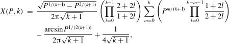 $$\begin{eqnarray}\displaystyle \displaystyle X(P,k) & = & \displaystyle \frac{\sqrt{P^{1/(k+1)}-P^{2/(k+1)}}}{2\unicode[STIX]{x03C0}\sqrt{k+1}}\left(\mathop{\prod }_{l=0}^{k-1}\frac{2+2l}{1+2l}\right)\mathop{\sum }_{m=0}^{k}\left(P^{m/(k+1)}\mathop{\prod }_{l=0}^{k-m-1}\frac{1+2l}{2+2l}\right)\nonumber\\ \displaystyle & & \displaystyle -\,\frac{\arcsin P^{1/(2(k+1))}}{2\unicode[STIX]{x03C0}\sqrt{k+1}}+\frac{1}{4\sqrt{k+1}},\end{eqnarray}$$
where $\unicode[STIX]{x1D6FE}=1+1/k$
;
$\unicode[STIX]{x1D6FE}=1+1/k$
; $1\leqslant k\leqslant 10$
. The requirement for
$1\leqslant k\leqslant 10$
. The requirement for $k$
to be an integer enables us to extract solutions over a working range of
$k$
to be an integer enables us to extract solutions over a working range of $1.10\leqslant \unicode[STIX]{x1D6FE}\leqslant 2.00$
. For the particular case of
$1.10\leqslant \unicode[STIX]{x1D6FE}\leqslant 2.00$
. For the particular case of $n=1$
, the list of exact solutions is presented in Table 1.
$n=1$
, the list of exact solutions is presented in Table 1.
Pressure relations for different values of the heat capacity ratio $\unicode[STIX]{x1D6FE}$
.
$\unicode[STIX]{x1D6FE}$
.

Equation (4.10) embodies the one-dimensional pressure distribution as a function of the axial distance. Its range of applicability ends at the point where choking occurs, which is accompanied by $\text{d}P/\text{d}X\rightarrow \infty$
, i.e. a condition that enables us to calculate the critical distance. Although not shown, the foregoing approximations obtained through an Abel inversion have been thoroughly verified numerically. Their use can provide an equivalent avenue for characterizing the flow field. For example, with the pressure distribution in hand, one can sample the data and solve for the radial distance numerically using
$\text{d}P/\text{d}X\rightarrow \infty$
, i.e. a condition that enables us to calculate the critical distance. Although not shown, the foregoing approximations obtained through an Abel inversion have been thoroughly verified numerically. Their use can provide an equivalent avenue for characterizing the flow field. For example, with the pressure distribution in hand, one can sample the data and solve for the radial distance numerically using
 $$\begin{eqnarray}\left(\frac{r}{a}\right)^{2}=2\sqrt{\frac{\unicode[STIX]{x1D6FE}-1}{\unicode[STIX]{x1D6FE}}}\int _{0}^{\unicode[STIX]{x1D701}}[P(\unicode[STIX]{x1D701}^{\prime })]^{n-1}\left[\frac{P(\unicode[STIX]{x1D701}^{\prime })}{P(X)}\right]^{1/\unicode[STIX]{x1D6FE}}\left[1-\left(\frac{P(X)}{P(\unicode[STIX]{x1D701}^{\prime })}\right)^{(\unicode[STIX]{x1D6FE}-1)/\unicode[STIX]{x1D6FE}}\right]^{-1/2}\text{d}\unicode[STIX]{x1D701}^{\prime },\end{eqnarray}$$
where all quantities on the right-hand side are known. The temperature may be similarly extracted from the isentropic relation, $T(x,\unicode[STIX]{x1D709})/[p(x)]^{(\unicode[STIX]{x1D6FE}-1)/\unicode[STIX]{x1D6FE}}=T_{w}(\unicode[STIX]{x1D709})/[p(\unicode[STIX]{x1D709})]^{(\unicode[STIX]{x1D6FE}-1)/\unicode[STIX]{x1D6FE}}$
. This enables us to retrieve the axial velocity using energy conservation,
$T(x,\unicode[STIX]{x1D709})/[p(x)]^{(\unicode[STIX]{x1D6FE}-1)/\unicode[STIX]{x1D6FE}}=T_{w}(\unicode[STIX]{x1D709})/[p(\unicode[STIX]{x1D709})]^{(\unicode[STIX]{x1D6FE}-1)/\unicode[STIX]{x1D6FE}}$
. This enables us to retrieve the axial velocity using energy conservation,
 $$\begin{eqnarray}u(x,\unicode[STIX]{x1D709})=\sqrt{2c_{p}[T_{w}(\unicode[STIX]{x1D709})-T(x,\unicode[STIX]{x1D709})]}.\end{eqnarray}$$
Subsequently, the radial component of the velocity may be evaluated from the continuity equation using forward-difference discretization. Finally, to calculate the Mach number, one may use (2.29).
5 Flow driven by oscillatory wall injection
Having verified the present formulation, its ability to accommodate various injection profiles can be immediately tested. Originally, the solution is developed for a propellant burning-rate behaviour that follows Saint-Robert’s power law. However, in modelling erosive burning of propellants, it is useful to explore the effects of varying the velocity profile along the injecting surface (Zhang & Jackson Reference Zhang and Jackson2010; Topalian et al.
Reference Topalian, Zhang, Jackson, Isfahani and Amir2011). This may be accomplished by first normalizing the variables $P(X)$
,
$P(X)$
, $X$
and
$X$
and $\unicode[STIX]{x1D701}$
with no pressure dependency. For this, we let:
$\unicode[STIX]{x1D701}$
with no pressure dependency. For this, we let:
 $$\begin{eqnarray}\displaystyle & \displaystyle P(X)=\frac{p(x)}{p_{0}}, & \displaystyle\end{eqnarray}$$
 $$\begin{eqnarray}\displaystyle & \displaystyle X=\sqrt{\frac{\unicode[STIX]{x1D6FE}}{\unicode[STIX]{x1D6FE}-1}}\frac{1}{a}\int _{0}^{x}\frac{U_{w}(x^{\prime })}{\sqrt{2c_{p}T_{w}(x^{\prime })}}\,\text{d}x^{\prime } & \displaystyle\end{eqnarray}$$
and
 $$\begin{eqnarray}\unicode[STIX]{x1D701}=\sqrt{\frac{\unicode[STIX]{x1D6FE}}{\unicode[STIX]{x1D6FE}-1}}\frac{1}{a}\int _{0}^{\unicode[STIX]{x1D709}}\frac{U_{w}(x^{\prime })}{\sqrt{2c_{p}T_{w}(x^{\prime })}}\,\text{d}x^{\prime }.\end{eqnarray}$$
Except for $P$
, the normalization process for
$P$
, the normalization process for $X$
and
$X$
and $\unicode[STIX]{x1D701}$
requires the use of their upper integral bounds. This group of coordinate distortions transforms (4.11) and (2.28) into
$\unicode[STIX]{x1D701}$
requires the use of their upper integral bounds. This group of coordinate distortions transforms (4.11) and (2.28) into
 $$\begin{eqnarray}\left(\frac{r}{a}\right)^{2}=2\sqrt{\frac{\unicode[STIX]{x1D6FE}-1}{\unicode[STIX]{x1D6FE}}}\int _{0}^{\unicode[STIX]{x1D701}}\left[\frac{P(\unicode[STIX]{x1D701}^{\prime })}{P(X)}\right]^{1/\unicode[STIX]{x1D6FE}}\left\{1-\left[\frac{P(X)}{P(\unicode[STIX]{x1D701}^{\prime })}\right]^{(\unicode[STIX]{x1D6FE}-1)/\unicode[STIX]{x1D6FE}}\right\}^{-1/2}\,\text{d}\unicode[STIX]{x1D701}^{\prime }\end{eqnarray}$$
and
 $$\begin{eqnarray}\sqrt{\frac{\unicode[STIX]{x1D6FE}}{\unicode[STIX]{x1D6FE}-1}}=2\int _{0}^{X}\left[\frac{P(\unicode[STIX]{x1D701})}{P(X)}\right]^{1/\unicode[STIX]{x1D6FE}}\left\{1-\left[\frac{P(X)}{P(\unicode[STIX]{x1D701})}\right]^{(\unicode[STIX]{x1D6FE}-1)/\unicode[STIX]{x1D6FE}}\right\}^{-1/2}\,\text{d}\unicode[STIX]{x1D701}.\end{eqnarray}$$
Equations (5.4) and (5.5) can be reproduced from (2.28) and (4.11) by suppressing the pressure dependency of the wall mass flux and setting $n=1$
. For the reader’s convenience, the resulting solutions are appended to Table 1.
$n=1$
. For the reader’s convenience, the resulting solutions are appended to Table 1.
Spatially oscillatory wall injection profile.

At this stage, an oscillatory velocity profile at the injecting wall may be imposed according to Zhang & Jackson (Reference Zhang and Jackson2010), as depicted in figure 11, using
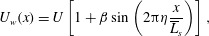 $$\begin{eqnarray}U_{w}(x)=U\left[1+\unicode[STIX]{x1D6FD}\sin \left(2\unicode[STIX]{x03C0}\unicode[STIX]{x1D702}\frac{x}{\overline{L}_{s}}\right)\right],\end{eqnarray}$$
where $\unicode[STIX]{x1D6FD}$
and
$\unicode[STIX]{x1D6FD}$
and $\unicode[STIX]{x1D702}$
are parameters that control the amplitude and the number of spatial wavelengths between
$\unicode[STIX]{x1D702}$
are parameters that control the amplitude and the number of spatial wavelengths between $x=0$
and
$x=0$
and $\overline{L}_{s}$
. Assuming a constant temperature along the sidewall, equation (5.2) can be integrated, given that
$\overline{L}_{s}$
. Assuming a constant temperature along the sidewall, equation (5.2) can be integrated, given that $U$
and
$U$
and $T_{w}$
are quantities which may be deduced from the characteristic wall Mach number. Next, the axial velocity may be determined in terms of
$T_{w}$
are quantities which may be deduced from the characteristic wall Mach number. Next, the axial velocity may be determined in terms of $x$
to account for the spatial oscillations.
$x$
to account for the spatial oscillations.
To examine the effect of the propellant burning-rate fluctuations on the flow, we start by computing the velocities with an oscillation amplitude of 30 % of the blowing speed (i.e. $\unicode[STIX]{x1D6FD}=0.3$
). We then subtract the outcome from a flow field driven by a uniform injection profile (of magnitude
$\unicode[STIX]{x1D6FD}=0.3$
). We then subtract the outcome from a flow field driven by a uniform injection profile (of magnitude $U$
). Results are given in figure 12 at different axial locations for (a)
$U$
). Results are given in figure 12 at different axial locations for (a) $\unicode[STIX]{x1D702}=5$
and (b)
$\unicode[STIX]{x1D702}=5$
and (b) $\unicode[STIX]{x1D702}=10$
. In this graph, the velocity magnitude is rescaled with respect to the centreline velocity; this auxiliary step makes it easier for us to visualize and infer the effects of burning-rate fluctuations. Axially, the propagation of disturbances becomes magnified in the streamwise direction, thus reaching a maximum decrement of 9.3 % (at the choking length) for
$\unicode[STIX]{x1D702}=10$
. In this graph, the velocity magnitude is rescaled with respect to the centreline velocity; this auxiliary step makes it easier for us to visualize and infer the effects of burning-rate fluctuations. Axially, the propagation of disturbances becomes magnified in the streamwise direction, thus reaching a maximum decrement of 9.3 % (at the choking length) for $\unicode[STIX]{x1D702}=5$
and 6.1 % for
$\unicode[STIX]{x1D702}=5$
and 6.1 % for $\unicode[STIX]{x1D702}=10$
. Conversely, the radial propagation of disturbances originating at the sidewall becomes less pronounced while moving downstream. Although the amplitude of oscillations is taken to be the same for both cases, higher wavenumbers lead to a more rapid attenuation of sidewall disturbances.
$\unicode[STIX]{x1D702}=10$
. Conversely, the radial propagation of disturbances originating at the sidewall becomes less pronounced while moving downstream. Although the amplitude of oscillations is taken to be the same for both cases, higher wavenumbers lead to a more rapid attenuation of sidewall disturbances.
Axial velocity fluctuations due to spatially oscillatory injection using (a) $\unicode[STIX]{x1D702}=5$
and (b) 10. Here
$\unicode[STIX]{x1D702}=5$
and (b) 10. Here $\unicode[STIX]{x1D6FD}=0.3$
and
$\unicode[STIX]{x1D6FD}=0.3$
and $\unicode[STIX]{x1D6FE}=1.33$
.
$\unicode[STIX]{x1D6FE}=1.33$
.

One can also study the pressure perturbations arising from this undulating boundary. Figure 13 showcases the pressure fluctuations being subtracted from the flow driven by uniform injection. On the one hand, results show an increase in pressure of up to 9.1 % for $\unicode[STIX]{x1D702}=5$
, while, on the other hand, the pressure is decreased by 1.6 % for
$\unicode[STIX]{x1D702}=5$
, while, on the other hand, the pressure is decreased by 1.6 % for $\unicode[STIX]{x1D702}=10$
. This unpredictable response of the pressure to surface irregularities or propellant burning-rate fluctuations warrants further examination. It also explains some of the challenging aspects that are often encountered when seeking to describe complex mechanisms such as erosive burning or resonant behaviour.
$\unicode[STIX]{x1D702}=10$
. This unpredictable response of the pressure to surface irregularities or propellant burning-rate fluctuations warrants further examination. It also explains some of the challenging aspects that are often encountered when seeking to describe complex mechanisms such as erosive burning or resonant behaviour.
Pressure fluctuations due to spatially oscillatory injection using (a) $\unicode[STIX]{x1D702}=5$
and (b) 10. Here
$\unicode[STIX]{x1D702}=5$
and (b) 10. Here $\unicode[STIX]{x1D6FD}=0.3$
and
$\unicode[STIX]{x1D6FD}=0.3$
and $\unicode[STIX]{x1D6FE}=1.33$
.
$\unicode[STIX]{x1D6FE}=1.33$
.
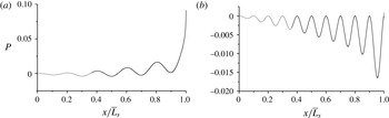
To explain the seemingly unpredictable response of the pressure, it is possible to evoke a concept that is traditionally used in stability characterization. Realizing that the amplitudes of the oscillatory pressure grow in one case and decay in the other, the fluctuations in question may be likened to the spatial coupling observed in the vicinity of resonant modes that arise in acoustical or vibrational analysis. Although the time-dependent formulation is not concerned with stability, it displays a behaviour that is characteristic of spatial stability problems. To better understand this analogy, we identify the resonant modes associated with a cylindrical cavity in which the acoustic frequencies correspond to the roots of $J_{\unicode[STIX]{x1D703}}^{\prime }(k_{\unicode[STIX]{x1D703}\unicode[STIX]{x1D702}})=0$
, where
$J_{\unicode[STIX]{x1D703}}^{\prime }(k_{\unicode[STIX]{x1D703}\unicode[STIX]{x1D702}})=0$
, where $J$
and
$J$
and $k$
denote the Bessel function of the first kind and the frequency, whereas
$k$
denote the Bessel function of the first kind and the frequency, whereas $\unicode[STIX]{x1D703}$
and
$\unicode[STIX]{x1D703}$
and $\unicode[STIX]{x1D702}$
allude to the tangential and radial mode numbers, respectively. In the axisymmetric case, where the tangential component is ignored, one takes
$\unicode[STIX]{x1D702}$
allude to the tangential and radial mode numbers, respectively. In the axisymmetric case, where the tangential component is ignored, one takes $\unicode[STIX]{x1D703}=0$
. In this context, the cases of
$\unicode[STIX]{x1D703}=0$
. In this context, the cases of $\unicode[STIX]{x1D702}=5$
and 10 display frequencies that fall close to the 10th and 20th modes, and these can naturally couple with the undulating injection velocity. It can thus be seen that the coupling between the spatial velocity oscillations and acoustic frequencies warrants a dedicated study that we hope to undertake in future work.
$\unicode[STIX]{x1D702}=5$
and 10 display frequencies that fall close to the 10th and 20th modes, and these can naturally couple with the undulating injection velocity. It can thus be seen that the coupling between the spatial velocity oscillations and acoustic frequencies warrants a dedicated study that we hope to undertake in future work.
A reacting solid propellant in a crossflow can suffer variations in its local burning rate, thus leading to erosive burning. Naturally, the wall shearing deformation rate becomes a parameter of interest when studying such variations along solid propellant grains (Jackson Reference Jackson2012). As defined by Topalian et al. (Reference Topalian, Zhang, Jackson, Isfahani and Amir2011), the wall shearing rate may be evaluated as the gradient of the streamwise velocity in the normal direction to the injecting surface, $(\text{d}u/\text{d}y)_{w}$
. In our case, figure 14 is used to compare the shear rate along the injecting surface for uniform wall injection as well as two undulating flows corresponding to
$(\text{d}u/\text{d}y)_{w}$
. In our case, figure 14 is used to compare the shear rate along the injecting surface for uniform wall injection as well as two undulating flows corresponding to $\unicode[STIX]{x1D702}=5$
and 10. Unsurprisingly, the uniformly injected motion displays the highest shearing rates at the endwall as the flow approaches choking conditions, where the streamwise-to-crossflow velocity ratio reaches its peak value. As for the undulating flow models, they too undergo a similar steepening of their shearing rates, with visible differences occurring between the
$\unicode[STIX]{x1D702}=5$
and 10. Unsurprisingly, the uniformly injected motion displays the highest shearing rates at the endwall as the flow approaches choking conditions, where the streamwise-to-crossflow velocity ratio reaches its peak value. As for the undulating flow models, they too undergo a similar steepening of their shearing rates, with visible differences occurring between the $\unicode[STIX]{x1D702}=5$
and 10 models as
$\unicode[STIX]{x1D702}=5$
and 10 models as $x/\overline{L}_{s}$
starts to exceed approximately 0.3. Physically, as the oscillatory frequency increases, the solution tends to approach that of a uniformly injected flow. This behaviour may be attributed to the reduced velocity oscillation amplitudes that accompany successive increases in
$x/\overline{L}_{s}$
starts to exceed approximately 0.3. Physically, as the oscillatory frequency increases, the solution tends to approach that of a uniformly injected flow. This behaviour may be attributed to the reduced velocity oscillation amplitudes that accompany successive increases in $\unicode[STIX]{x1D702}$
, as confirmed in figure 12(b).
$\unicode[STIX]{x1D702}$
, as confirmed in figure 12(b).
Comparison of the shear deformation rate along the injecting surface for three cases corresponding to: uniform injection, oscillatory injection with $\unicode[STIX]{x1D702}=5$
, and oscillatory injection with
$\unicode[STIX]{x1D702}=5$
, and oscillatory injection with $\unicode[STIX]{x1D702}=10$
.
$\unicode[STIX]{x1D702}=10$
.

By virtue of this example, the effectiveness of the present framework in reproducing variable surface injection conditions is showcased using a spatially oscillatory sidewall injection pattern. In a more dedicated study, such capability may be more thoroughly invested in modelling the erosive burning mechanism that affects propellant regression. For example, by comparing the velocity and pressure fluctuations at different spatial wavenumbers, it may be seen that a lower wavenumber can have a greater impact on the pressure amplitude.
6 Conclusions
In this article, the integral formulation of the axisymmetric porous cylinder, which was initiated by Traineau et al. (Reference Traineau, Hervat and Kuentzmann1986) in the context of a planar, two-dimensional flow analogue, is carefully reconstructed and compared to one- and two-dimensional analytical solutions obtained under isentropic and homentropic flow conditions. At the outset, we find that the level of agreement between the closed-form approximations and the integral representation is consistent with the sidewall boundary conditions associated with each of these models. Being derived for a uniform mass flux at the sidewall, the one-dimensional model seems to provide a better estimate of the inverted integral at a pressure exponent of $n=0$
. Such a condition suppresses the velocity dependence on the pressure and ensures a constant mass flux at the sidewall. Conversely, the
$n=0$
. Such a condition suppresses the velocity dependence on the pressure and ensures a constant mass flux at the sidewall. Conversely, the $n=1$
case leads to a constant wall-normal velocity, which coincides with one of the boundary conditions used in constructing the axisymmetric analytical model of Majdalani (Reference Majdalani2007). Numerical predictions for this case using a strictly inviscid, compressible solver fall in close agreement with the present formulation.
$n=1$
case leads to a constant wall-normal velocity, which coincides with one of the boundary conditions used in constructing the axisymmetric analytical model of Majdalani (Reference Majdalani2007). Numerical predictions for this case using a strictly inviscid, compressible solver fall in close agreement with the present formulation.
In all cases considered, the main discrepancies arise near the sonic point, where disparities may be attributed to the various forms of irreversibilities. Furthermore, when comparing the level of difficulty needed to reproduce these solutions, the closed-form analytical approximations seem to substantially outperform the semi-analytical techniques. The latter require piecewise numerical integrations, sequential inversions, and backward transformations to retrieve the original variables of interest. The problem is further exacerbated by the variable extraction process occurring over a highly non-uniform mesh. The ensuing operation can render simple steps extraordinarily challenging, especially when attempting to extrapolate related variables and derivatives that are needed over a uniform grid. Such effort can prove to be laborious when compared to the ease with which the strictly analytical models are implemented and resolved. Nonetheless, the integral formulation remains essential for a number of reasons. For example, unlike the analytical models, it is not limited to uniform wall injection profiles in mass flux or velocity. On the contrary, it enables us to expeditiously solve for the compressible motion in the presence of an arbitrary wall injection pattern. Furthermore, it helps to confirm several useful characteristics associated with the two-dimensional theory introduced previously (Majdalani Reference Majdalani2007). Among them is the strong, albeit non-exact, self-similarity with respect to the critical length. This can be realized by rescaling the axial coordinate with respect to $x=L_{s}$
. Following such renormalization, numerically obtained streamlines, pressures, and temperatures at two different Mach numbers become virtually identical when graphically displayed. The resulting behaviour is consistent with the projections of two-dimensional theory, namely, that deviations from self-similarity appear at the order of the wall Mach number squared, a practically small quantity that induces relative differences that fall below 1 %.
$x=L_{s}$
. Following such renormalization, numerically obtained streamlines, pressures, and temperatures at two different Mach numbers become virtually identical when graphically displayed. The resulting behaviour is consistent with the projections of two-dimensional theory, namely, that deviations from self-similarity appear at the order of the wall Mach number squared, a practically small quantity that induces relative differences that fall below 1 %.
In addition to the numerical treatment of the reduced-order integral formulation, an Abel transformation is implemented in this study to produce an exact expression for the pressure distribution at several distinct values of the heat capacity ratio $\unicode[STIX]{x1D6FE}$
. This enables us to retrieve two sets of explicit solutions linking the pressure and the axial location within the chamber: the first corresponds to a uniformly injecting mass flux with
$\unicode[STIX]{x1D6FE}$
. This enables us to retrieve two sets of explicit solutions linking the pressure and the axial location within the chamber: the first corresponds to a uniformly injecting mass flux with $n=0$
, and, the second, to a uniformly injecting velocity with
$n=0$
, and, the second, to a uniformly injecting velocity with $n=1$
. While the former is shown to be reproducible from a general recursive relation, the latter may be expressed as a finite-term expansion for each viable ratio of specific heats. Being exact, the ensuing formulations provide an alternate avenue for verifying the outcome of numerical integration, thus confirming the steepening of the velocity profiles and their gradients in the vicinity of the sidewall. They also increase our repertoire of compressible flow approximations over a generous range of
$n=1$
. While the former is shown to be reproducible from a general recursive relation, the latter may be expressed as a finite-term expansion for each viable ratio of specific heats. Being exact, the ensuing formulations provide an alternate avenue for verifying the outcome of numerical integration, thus confirming the steepening of the velocity profiles and their gradients in the vicinity of the sidewall. They also increase our repertoire of compressible flow approximations over a generous range of $1.10\leqslant \unicode[STIX]{x1D6FE}\leqslant 2.0$
.
$1.10\leqslant \unicode[STIX]{x1D6FE}\leqslant 2.0$
.
In closing, the ability of the present framework to accommodate a variable wall injection function is illustrated using a spatially undulating velocity. The corresponding phenomenological problem is connected to the erosive burning phenomenon, which often arises in the context of combustion instability. Despite the variable injection speed along the length of the chamber, a numerical solution is obtained rather straightforwardly using the model with $n=1$
. This example showcases the versatility of the present framework in handling an arbitrarily specified injection pattern that may be the outcome of an idealized physical mechanism. In future work, we plan to extend the present formulation to non-isentropic conditions and to other physical settings that encompass simulated hybrid rocket chambers, and both Beltramian and Trkalian families of compressible mean-flow solutions that arise in the context of swirling solid rocket motor flows as well as cyclonically driven, bidirectional vortex chambers. We also hope to further explore the erosive burning mechanism through the use of suitably constructed sidewall injection patterns.
$n=1$
. This example showcases the versatility of the present framework in handling an arbitrarily specified injection pattern that may be the outcome of an idealized physical mechanism. In future work, we plan to extend the present formulation to non-isentropic conditions and to other physical settings that encompass simulated hybrid rocket chambers, and both Beltramian and Trkalian families of compressible mean-flow solutions that arise in the context of swirling solid rocket motor flows as well as cyclonically driven, bidirectional vortex chambers. We also hope to further explore the erosive burning mechanism through the use of suitably constructed sidewall injection patterns.
Acknowledgements
This material is based on work that was supported partly by the National Science Foundation and partly by the Hugh and Loeda Francis Chair of Excellence, Department of Aerospace Engineering, Auburn University. The authors thank T. R. Kumar and G. Sharma for their valuable assistance in revising the manuscript.
Appendix A
According to Majdalani (Reference Majdalani2007), the compressible mean-flow motion that develops under inviscid conditions in a porous tube as a result of a uniformly distributed sidewall injection velocity may be expressed in dimensionless form using
 $$\begin{eqnarray}\displaystyle & \hspace{-3.0pt}\displaystyle \unicode[STIX]{x1D713}=M_{w}\unicode[STIX]{x1D713}_{0}\!\left(1-\textstyle \frac{1}{4}\unicode[STIX]{x1D6E4}^{2}\!\left[1+\textstyle \frac{1}{3}\cos (\unicode[STIX]{x03C0}r^{2})\right]\!\unicode[STIX]{x1D712}^{2}\!+\textstyle \frac{1}{2}M_{w}^{2}\right)\!;\!\quad \unicode[STIX]{x1D713}_{0}=x\sin \!\left(\textstyle \frac{1}{2}\unicode[STIX]{x03C0}r^{2}\right)\!\quad \text{(streamfunction)}\hspace{-3.0pt} & \displaystyle \nonumber\\ \displaystyle & & \displaystyle\end{eqnarray}$$
and
 $$\begin{eqnarray}\displaystyle & \displaystyle M_{c}=\unicode[STIX]{x1D6E4}\frac{2+\textstyle \frac{1}{3}\unicode[STIX]{x1D6E4}^{2}\unicode[STIX]{x1D712}^{2}-M_{w}^{2}}{\sqrt{4-2(\unicode[STIX]{x1D6FE}-1)\unicode[STIX]{x1D6E4}^{2}\unicode[STIX]{x1D712}^{2}}}\unicode[STIX]{x1D712}\quad \text{(centreline Mach number)},\qquad & \displaystyle\end{eqnarray}$$
 $$\begin{eqnarray}\displaystyle & \displaystyle p_{c}=1-\textstyle \frac{1}{2}\unicode[STIX]{x1D6FE}\,\unicode[STIX]{x1D6E4}^{2}\unicode[STIX]{x1D712}^{2}(1-M_{w}^{2})-\textstyle \frac{1}{24}\unicode[STIX]{x1D6FE}\,\unicode[STIX]{x1D6E4}^{4}\unicode[STIX]{x1D712}^{4}\quad \text{(centreline pressure)},\qquad & \displaystyle\end{eqnarray}$$
 $$\begin{eqnarray}\displaystyle & \displaystyle T_{c}=1-\textstyle \frac{1}{2}(\unicode[STIX]{x1D6FE}-1)\unicode[STIX]{x1D6E4}^{2}\unicode[STIX]{x1D712}^{2}(1-M_{w}^{2})-\textstyle \frac{1}{6}(\unicode[STIX]{x1D6FE}-1)\unicode[STIX]{x1D6E4}^{4}\unicode[STIX]{x1D712}^{4}\quad \text{(centreline temperature)},\qquad & \displaystyle\end{eqnarray}$$
where the sonic length, $L_{s}$
, also known as the critical distance, is related to the
$L_{s}$
, also known as the critical distance, is related to the $\unicode[STIX]{x1D6E4}$
function through
$\unicode[STIX]{x1D6E4}$
function through
 $$\begin{eqnarray}\displaystyle \unicode[STIX]{x1D6E4} & \equiv & \displaystyle \unicode[STIX]{x03C0}M_{w}L_{s}=\sqrt{\unicode[STIX]{x1D706}-2\unicode[STIX]{x1D6FE}-2+2(2\unicode[STIX]{x1D6FE}^{2}+\unicode[STIX]{x1D6FE}-1)/\unicode[STIX]{x1D706}}\nonumber\\ \displaystyle & \cong & \displaystyle 0.884622-0.177299(\unicode[STIX]{x1D6FE}-1)+0.0539119(\unicode[STIX]{x1D6FE}-1)^{2}-0.0180615(\unicode[STIX]{x1D6FE}-1)^{3}\qquad\end{eqnarray}$$
and
 $$\begin{eqnarray}\unicode[STIX]{x1D706}=\left(28+12\unicode[STIX]{x1D6FE}-6\unicode[STIX]{x1D6FE}^{2}-8\unicode[STIX]{x1D6FE}^{3}+6\sqrt{22+18\unicode[STIX]{x1D6FE}-6\unicode[STIX]{x1D6FE}^{2}-14\unicode[STIX]{x1D6FE}^{3}-3\unicode[STIX]{x1D6FE}^{4}}\right)^{1/3}.\end{eqnarray}$$


 Open access