





1. Introduction
Turbulent convection is ubiquitous in nature. Driven by thermal or chemical gradients, this buoyancy-induced motion occurs throughout the atmospheres and interiors of rotating celestial bodies (Marshall & Schott Reference Marshall and Schott1999; Roberts & King Reference Roberts and King2013). In these systems, the competition between Coriolis-driven columnar structures and buoyant plumes dictates the mixing dynamics of atmospheres, mantles and cores (Emanuel Reference Emanuel1994; Aurnou et al. Reference Aurnou, Calkins, Cheng, Julien, King, Nieves, Soderlund and Stellmach2015). While the relative strength of these forces is traditionally characterised by the Rayleigh ( $R$
) and Ekman (
$R$
) and Ekman ( $E$
) numbers, a fundamental challenge in accurately modelling these environments lies in the extreme diversity of the fluid properties themselves. In particular, in nature there is a vast range of Prandtl numbers (
$E$
) numbers, a fundamental challenge in accurately modelling these environments lies in the extreme diversity of the fluid properties themselves. In particular, in nature there is a vast range of Prandtl numbers ( $\textit{Pr}$
), i.e. the ratio of viscous to thermal diffusion, ranging from being
$\textit{Pr}$
), i.e. the ratio of viscous to thermal diffusion, ranging from being $O(1)$
in atmospheres and
$O(1)$
in atmospheres and $10^{-1}$
to
$10^{-1}$
to $10^{-2}$
in liquid iron cores to
$10^{-2}$
in liquid iron cores to ${\sim} 10^{23}$
in planetary mantles. Such variations fundamentally alter how heat is processed and how rotation constrains the flow.
${\sim} 10^{23}$
in planetary mantles. Such variations fundamentally alter how heat is processed and how rotation constrains the flow.
The canonical model used to describe rotating convection is the Boussinesq approximation to the Navier–Stokes equations in a rotating frame, where the centrifugal force is neglected under either a constant density or small-rotation assumptions (Ecke & Shishkina Reference Ecke and Shishkina2023). While the vast majority of literature focuses on convection driven by boundary temperature gradients in the classic Rayleigh–Bénard (RB) problem (Chandrasekhar Reference Chandrasekhar1953; Veronis Reference Veronis1959; Grossmann & Lohse Reference Grossmann and Lohse2000; Vorobieff & Ecke Reference Vorobieff and Ecke2002; Stevens, Clercx & Lohse Reference Stevens, Clercx and Lohse2013; Kunnen Reference Kunnen2021; Ecke & Shishkina Reference Ecke and Shishkina2023; Lohse & Shishkina Reference Lohse and Shishkina2024), we instead focus on internally heated convection (IHC) between two perfectly conducting horizontal boundaries, where the fluid is heated volumetrically (Roberts Reference Roberts1967; Tritton & Zarraga Reference Tritton and Zarraga1967; Thirlby Reference Thirlby1970; Kulacki & Goldstein Reference Kulacki and Goldstein1972; Goluskin & Spiegel Reference Goluskin and Spiegel2012; Goluskin & Van der Poel Reference Goluskin and Van der Poel2016; Bouillaut et al. Reference Bouillaut, Miquel, Julien, Aumaître and Gallet2021; Hadjerci et al. Reference Hadjerci, Bouillaut, Miquel and Gallet2024). This configuration is fundamentally different from the classic RB problem in several ways. Notably, IHC supports subcritical convection; the Rayleigh number determining the energy stability limit ( $R_E\approx 26\,926.6$
for no-slip boundaries) is significantly lower than the Rayleigh number determining the linear instability threshold (
$R_E\approx 26\,926.6$
for no-slip boundaries) is significantly lower than the Rayleigh number determining the linear instability threshold ( $R_L\approx 37\,325.2$
), whereas RB convection onsets via a pitchfork bifurcation at
$R_L\approx 37\,325.2$
), whereas RB convection onsets via a pitchfork bifurcation at $R_E=R_L\approx 1707.76$
(Chandrasekhar Reference Chandrasekhar1961; Goluskin Reference Goluskin2016). In addition, because heat is not transported from one boundary to the other, the standard Nusselt number used in RB studies (Lohse & Shishkina Reference Lohse and Shishkina2023) is not applicable. Instead, two global quantities are used to assess the effectiveness of convection: the mean temperature
$R_E=R_L\approx 1707.76$
(Chandrasekhar Reference Chandrasekhar1961; Goluskin Reference Goluskin2016). In addition, because heat is not transported from one boundary to the other, the standard Nusselt number used in RB studies (Lohse & Shishkina Reference Lohse and Shishkina2023) is not applicable. Instead, two global quantities are used to assess the effectiveness of convection: the mean temperature $\overline {\langle T \rangle }$
and the bottom heat flux heat fraction
$\overline {\langle T \rangle }$
and the bottom heat flux heat fraction $\mathcal{F}_B$
, where
$\mathcal{F}_B$
, where $\langle \cdot\rangle$
denotes averaging in the horizontal directions and time, and the overbar
$\langle \cdot\rangle$
denotes averaging in the horizontal directions and time, and the overbar $\overline{\phi}$
denotes averages in the vertical direction.
$\overline{\phi}$
denotes averages in the vertical direction.
In IHC, turbulence serves a dual role: it homogenises the bulk temperature field while simultaneously creating an asymmetry in the heat flux leaving the boundaries, a flux that is perfectly balanced in the purely conductive state (Arslan et al. Reference Arslan, Fantuzzi, Craske and Wynn2021). This asymmetry results in an unstably stratified thermal boundary layer at the top and a stably stratified layer at the bottom. The distinct structures of these layers contribute to scaling laws for viscous dissipation that remain less understood than their thermal counterparts (Wang, Lohse & Shishkina Reference Wang, Lohse and Shishkina2020; Arslan & Rojas Reference Arslan and Rojas2025), with evidence suggesting that the viscous dissipation scales differently between two- and three-dimensional systems (Goluskin & Van der Poel Reference Goluskin and Van der Poel2016; Ostilla-Mónico & Arslan Reference Ostilla-Mónico and Arslan2025).
The disparity between the top and bottom boundary layers is further accentuated by rotation. In rotating RB convection (RRBC), the relative thicknesses of thermal and viscous boundary layers serve as a key diagnostic for identifying the transition from buoyancy-dominated flow to geostrophic turbulence (King et al. Reference King, Stellmach, Noir, Hansen and Aurnou2009; Maffei et al. Reference Maffei, Krouss, Julien and Calkins2021). A hallmark of this transition is the emergence and subsequent decoherence of Taylor columns as the rotation rate increases (Grooms et al. Reference Grooms, Julien, Weiss and Knobloch2010; Kunnen et al. Reference Kunnen, Ostilla-Mónico, Van Der Poel, Verzicco and Lohse2016). However, in rotating IHC, the stable bottom stratification interacts with the Ekman boundary layer, a phenomenon absent in boundary-driven systems which complicates the picture (Ostilla-Mónico & Arslan Reference Ostilla-Mónico and Arslan2025). The effect of $\textit{Pr}$
on this phenomenon is yet to be revealed.
$\textit{Pr}$
on this phenomenon is yet to be revealed.
The morphology of these flows is also heavily dictated by the Prandtl number. In the limits of $\textit{Pr}\to \infty$
and
$\textit{Pr}\to \infty$
and $\textit{Pr}\to 0$
, the momentum equation approaches forced Stokes and Euler flows, respectively. While
$\textit{Pr}\to 0$
, the momentum equation approaches forced Stokes and Euler flows, respectively. While $\textit{Pr}$
effects have been extensively documented for RRBC (King & Aurnou Reference King and Aurnou2013; Horn & Schmid Reference Horn and Schmid2017; Aurnou et al. Reference Aurnou, Bertin, Grannan, Horn and Vogt2018; Vogt et al. Reference Vogt, Horn, Grannan and Aurnou2018; Abbate & Aurnou Reference Abbate and Aurnou2023; Fan, Wang & Lin Reference Fan, Wang and Lin2024; Xu et al. Reference Xu, Abbate, David, Vogt and Aurnou2025), the low-
$\textit{Pr}$
effects have been extensively documented for RRBC (King & Aurnou Reference King and Aurnou2013; Horn & Schmid Reference Horn and Schmid2017; Aurnou et al. Reference Aurnou, Bertin, Grannan, Horn and Vogt2018; Vogt et al. Reference Vogt, Horn, Grannan and Aurnou2018; Abbate & Aurnou Reference Abbate and Aurnou2023; Fan, Wang & Lin Reference Fan, Wang and Lin2024; Xu et al. Reference Xu, Abbate, David, Vogt and Aurnou2025), the low- $\textit{Pr}$
regime is computationally demanding and remains relatively unexplored for IHC. One critical feature of RRBC that vanishes at low
$\textit{Pr}$
regime is computationally demanding and remains relatively unexplored for IHC. One critical feature of RRBC that vanishes at low $\textit{Pr}$
is the rotational enhancement of heat transport. In RB systems, this enhancement is attributed to Ekman pumping, which becomes ineffective at low Pr as high thermal diffusivity allows heat to escape the boundary layers before it can be vertically transported (Stevens et al. Reference Stevens, Clercx and Lohse2010a
). Whether this suppression of transport enhancement persists in internally heated systems, where the driving is volumetric rather than boundary-based, remains an open question.
$\textit{Pr}$
is the rotational enhancement of heat transport. In RB systems, this enhancement is attributed to Ekman pumping, which becomes ineffective at low Pr as high thermal diffusivity allows heat to escape the boundary layers before it can be vertically transported (Stevens et al. Reference Stevens, Clercx and Lohse2010a
). Whether this suppression of transport enhancement persists in internally heated systems, where the driving is volumetric rather than boundary-based, remains an open question.
This paper builds upon the work of Ostilla-Mónico & Arslan (Reference Ostilla-Mónico and Arslan2025) to provide the first direct numerical simulations of low- $\textit{Pr}$
to high-
$\textit{Pr}$
to high- $\textit{Pr}$
rotating IHC. We conduct a parametric study across a wide range of
$\textit{Pr}$
rotating IHC. We conduct a parametric study across a wide range of $R$
and
$R$
and $E$
to quantify the bulk responses, horizontally averaged profiles and boundary-layer dynamics of this unique system. The paper is organised as follows. Section 2 describes the governing equations and simulation method. In § 3, we present results for the variation of
$E$
to quantify the bulk responses, horizontally averaged profiles and boundary-layer dynamics of this unique system. The paper is organised as follows. Section 2 describes the governing equations and simulation method. In § 3, we present results for the variation of $\textit{Pr}$
on non-rotating IHC, while § 4 contains results for the effect of
$\textit{Pr}$
on non-rotating IHC, while § 4 contains results for the effect of $\textit{Pr}$
on rotating IHC. Finally, § 5 briefly summarises the results obtained.
$\textit{Pr}$
on rotating IHC. Finally, § 5 briefly summarises the results obtained.
2. Set-up
In this study, IHC is examined within a fluid layer of depth $d$
, bounded by two horizontal plates, as shown in figure 1. We assume periodic boundary conditions in the horizontal dimensions with a domain aspect ratio of
$d$
, bounded by two horizontal plates, as shown in figure 1. We assume periodic boundary conditions in the horizontal dimensions with a domain aspect ratio of $\varGamma d$
. The physical properties of the fluid, i.e. the kinematic viscosity
$\varGamma d$
. The physical properties of the fluid, i.e. the kinematic viscosity $\nu$
, the thermal diffusivity
$\nu$
, the thermal diffusivity $\kappa$
, the density
$\kappa$
, the density $\rho$
, the specific heat
$\rho$
, the specific heat $c_p$
and the thermal expansion coefficient
$c_p$
and the thermal expansion coefficient $\alpha$
, are assumed constant. The system undergoes uniform internal heating at a rate
$\alpha$
, are assumed constant. The system undergoes uniform internal heating at a rate $H$
, and rotates at a constant angular velocity
$H$
, and rotates at a constant angular velocity $\varOmega$
about the vertical axis, with gravity
$\varOmega$
about the vertical axis, with gravity $g$
acting downward. We employ the Boussinesq approximation to account for density variations solely through the buoyancy term.
$g$
acting downward. We employ the Boussinesq approximation to account for density variations solely through the buoyancy term.
A non-dimensional schematic diagram for rotating uniform IHC. The upper and lower plates are at the same temperature, and the domain is periodic in the $x$
and
$x$
and $y$
directions and rotates about the
$y$
directions and rotates about the $z$
axis. Fluxes
$z$
axis. Fluxes $\mathcal{F}_B$
and
$\mathcal{F}_B$
and $\mathcal{F}_T$
are the mean heat fluxes out of the bottom and top plates,
$\mathcal{F}_T$
are the mean heat fluxes out of the bottom and top plates, $\overline {\langle T \rangle }$
is the mean temperature and
$\overline {\langle T \rangle }$
is the mean temperature and $g$
is the acceleration due to gravity.
$g$
is the acceleration due to gravity.

Following the scaling convention of Roberts (Reference Roberts1967), the system is non-dimensionalised using $d$
for length,
$d$
for length, $d^2/\kappa$
for time and
$d^2/\kappa$
for time and $d^2H/(\kappa \rho c_p)$
for temperature. Under this non-dimensionalisation, the evolution of the velocity field
$d^2H/(\kappa \rho c_p)$
for temperature. Under this non-dimensionalisation, the evolution of the velocity field $\boldsymbol{u}(\boldsymbol{x},t)=u(\boldsymbol{x},t)\boldsymbol{e}_1+v(\boldsymbol{x},t)\boldsymbol{e}_2+w(\boldsymbol{x},t)\boldsymbol{e}_3$
and temperature field
$\boldsymbol{u}(\boldsymbol{x},t)=u(\boldsymbol{x},t)\boldsymbol{e}_1+v(\boldsymbol{x},t)\boldsymbol{e}_2+w(\boldsymbol{x},t)\boldsymbol{e}_3$
and temperature field $T(\boldsymbol{x},t)$
is governed by the following equations:
$T(\boldsymbol{x},t)$
is governed by the following equations:
 \begin{align} &\hspace{7pc} \boldsymbol{\nabla }\boldsymbol{\cdot }\boldsymbol{u}=0, \\[-12pt]\nonumber \end{align}
 \begin{align} &\partial _t \boldsymbol{u} + \boldsymbol{u}\boldsymbol{\cdot }\boldsymbol{\nabla }\boldsymbol{u} + E^{-1} \boldsymbol{e}_3 \times \boldsymbol{u} = -\boldsymbol{\nabla }\!p + \textit{Pr} {\nabla} ^2\boldsymbol{u} + \textit{Pr} \textit{RT} \boldsymbol{e}_3, \\[-12pt]\nonumber \end{align}
 \begin{align} &\def\lumina\hspace{5.5pc} \partial _tT + \boldsymbol{u}\boldsymbol{\cdot }\boldsymbol{\nabla }T = {\nabla} ^2 T +1 . \end{align}
The velocity and temperature fields are constrained by no-slip ( $\boldsymbol{u}=0$
) and isothermal (
$\boldsymbol{u}=0$
) and isothermal ( $T=0$
) conditions at both the upper and lower boundaries.
$T=0$
) conditions at both the upper and lower boundaries.
The dynamical response of the system is determined by three fundamental dimensionless groups: the Rayleigh number ( $R$
), the Ekman number (
$R$
), the Ekman number ( $E$
) and the Prandtl number (
$E$
) and the Prandtl number ( $\textit{Pr}$
):
$\textit{Pr}$
):
 \begin{equation} R = \frac {g\alpha Hd^5}{\rho c_p \nu \kappa ^2}, \quad E=\frac {\nu }{2\varOmega d^2}, \quad \textit{Pr}=\frac {\nu }{\kappa }. \end{equation}
Additionally, we can obtain the convective Rossby number, $Ro=E\sqrt {R/\textit{Pr}}$
, to quantify the competition between buoyant and Coriolis forces.
$Ro=E\sqrt {R/\textit{Pr}}$
, to quantify the competition between buoyant and Coriolis forces.
The governing equations (2.1)–(2.3) are numerically integrated using AFiD (Van Der Poel et al. Reference Van Der Poel, Ostilla-Mónico, Donners and Verzicco2015). This open-source code employs a second-order centred finite-difference scheme and has been thoroughly benchmarked for internal heating scenarios (Goluskin & Van der Poel Reference Goluskin and Van der Poel2016; Kazemi, Ostilla-Mónico & Goluskin Reference Kazemi, Ostilla-Mónico and Goluskin2022; Ostilla-Mónico & Arslan Reference Ostilla-Mónico and Arslan2025).
In this study, we extend the results of Ostilla-Mónico & Arslan (Reference Ostilla-Mónico and Arslan2025) by varying the Prandtl number to explore the ( $\textit{Pr}$
,
$\textit{Pr}$
, $R$
,
$R$
, $E$
) parameter space of rotationally affected convection. We vary
$E$
) parameter space of rotationally affected convection. We vary $\textit{Pr}$
in the range
$\textit{Pr}$
in the range $\textit{Pr}\in [0.1,10]$
,
$\textit{Pr}\in [0.1,10]$
, $R$
in the range
$R$
in the range $R\in [3.16\times 10^5,10^{10}]$
and
$R\in [3.16\times 10^5,10^{10}]$
and $E\in [10^{-6},\infty ]$
. To be more specific, we extend the parameter space explored in Ostilla-Mónico & Arslan (Reference Ostilla-Mónico and Arslan2025) by repeating the
$E\in [10^{-6},\infty ]$
. To be more specific, we extend the parameter space explored in Ostilla-Mónico & Arslan (Reference Ostilla-Mónico and Arslan2025) by repeating the $(R,E)$
pairs for four different values of
$(R,E)$
pairs for four different values of $\textit{Pr}$
:
$\textit{Pr}$
: $\textit{Pr}=0.1$
,
$\textit{Pr}=0.1$
, $0.3$
,
$0.3$
, $3$
and
$3$
and $10$
. We also run a series of non-rotating cases (
$10$
. We also run a series of non-rotating cases ( $E=\infty$
) for
$E=\infty$
) for $\textit{Pr}=30$
and
$\textit{Pr}=30$
and $100$
for
$100$
for $R \in [10^6, 10^10]$
.
$R \in [10^6, 10^10]$
.
The non-dimensional periodicity length $\varGamma$
is selected following the values of Ostilla-Mónico & Arslan (Reference Ostilla-Mónico and Arslan2025) for the
$\varGamma$
is selected following the values of Ostilla-Mónico & Arslan (Reference Ostilla-Mónico and Arslan2025) for the $\textit{Pr}=1$
cases, except for
$\textit{Pr}=1$
cases, except for $R=10^9$
where
$R=10^9$
where $\varGamma$
is reduced to 1. For
$\varGamma$
is reduced to 1. For $\textit{Pr}\geqslant 1$
, this ensures that
$\textit{Pr}\geqslant 1$
, this ensures that $\overline {\langle T \rangle }$
and
$\overline {\langle T \rangle }$
and $\overline {\langle wT \rangle }$
remain independent of domain size. For
$\overline {\langle wT \rangle }$
remain independent of domain size. For $\textit{Pr}\leqslant 1$
, a dependence of
$\textit{Pr}\leqslant 1$
, a dependence of $\overline {\langle wT \rangle }$
on the horizontal periodicity length
$\overline {\langle wT \rangle }$
on the horizontal periodicity length $\varGamma$
is introduced. While this does not change the overall physics of the problem, we quantify its effect in Appendix A.
$\varGamma$
is introduced. While this does not change the overall physics of the problem, we quantify its effect in Appendix A.
The resolution adequacy is measured by the following exact relationships:
 \begin{align} \overline {\langle \epsilon _\nu \rangle } \equiv \overline {\langle | \boldsymbol{\nabla }\boldsymbol{u}|^2 \rangle } = R\overline {\langle wT\rangle }, \end{align}
 \begin{align} \overline {\langle \epsilon _\theta \rangle } \equiv \overline {\langle |\boldsymbol{\nabla }T|^2\rangle } = \overline {\langle T \rangle } . \end{align}
To guarantee numerical accuracy, we ensure that both sides of the equation do not deviate by more than 1 %. This criterion provides a more stringent resolution constraint than those based solely on the mean Kolmogorov or Batchelor scales, yet it is recognised as sufficient for characterising thermal convection (Stevens et al. Reference Stevens, Verzicco and Lohse2010b ).
We base our resolutions on the values used Ostilla-Mónico & Arslan (Reference Ostilla-Mónico and Arslan2025), which satisfy the criteria above for all $\textit{Pr}$
. These yield grids from
$\textit{Pr}$
. These yield grids from $288^2\times 144$
points to the largest grid of
$288^2\times 144$
points to the largest grid of $384^2\times 512$
. As a general rule, the number of points in the vertical direction increases as
$384^2\times 512$
. As a general rule, the number of points in the vertical direction increases as $E$
becomes smaller, while the number of points in the horizontal direction does not vary as much because the required periodicity length
$E$
becomes smaller, while the number of points in the horizontal direction does not vary as much because the required periodicity length $\varGamma$
decreases with
$\varGamma$
decreases with $R$
, so grid resolution is increased despite keeping the same number of points. In the most adverse cases, the discretisation used in this paper has a maximum point distance of
$R$
, so grid resolution is increased despite keeping the same number of points. In the most adverse cases, the discretisation used in this paper has a maximum point distance of $1.5$
Kolmogorov length scales. In the non-rotating case, the upper thermal boundary layer, whose extent can be estimated by
$1.5$
Kolmogorov length scales. In the non-rotating case, the upper thermal boundary layer, whose extent can be estimated by $\langle \overline {T}\rangle /(({1}/{2})+\overline {\langle wT \rangle } )$
is resolved by at least six points. As rotation increases, the number of points in the
$\langle \overline {T}\rangle /(({1}/{2})+\overline {\langle wT \rangle } )$
is resolved by at least six points. As rotation increases, the number of points in the $z$
direction must be increased to resolve the increasingly thinner Ekman (velocity) boundary layers. A full list of all the resolutions used for the new simulations can be found in Appendix B.
$z$
direction must be increased to resolve the increasingly thinner Ekman (velocity) boundary layers. A full list of all the resolutions used for the new simulations can be found in Appendix B.
For $\textit{Pr}=0.3$
and
$\textit{Pr}=0.3$
and $\textit{Pr}=3$
, simulations are initialised from initial conditions at
$\textit{Pr}=3$
, simulations are initialised from initial conditions at $\textit{Pr}=1$
with the same (
$\textit{Pr}=1$
with the same ( $R$
,
$R$
, $E$
) parameter values, while for
$E$
) parameter values, while for $\textit{Pr}=0.1$
and
$\textit{Pr}=0.1$
and $\textit{Pr}=10$
they are started from the
$\textit{Pr}=10$
they are started from the $\textit{Pr}=0.3$
and
$\textit{Pr}=0.3$
and $\textit{Pr}=3$
cases, respectively. After transients, statistics are collected for a time interval of length
$\textit{Pr}=3$
cases, respectively. After transients, statistics are collected for a time interval of length $t_{av}$
which ensure that the time-averaged values of
$t_{av}$
which ensure that the time-averaged values of $\overline {\langle T \rangle }$
and
$\overline {\langle T \rangle }$
and $\overline {\langle wT \rangle }$
are less than 1
$\overline {\langle wT \rangle }$
are less than 1 $\%$
different from those corresponding to half the run time. In general
$\%$
different from those corresponding to half the run time. In general $t_{av}$
depends on both
$t_{av}$
depends on both $\textit{Pr}$
and
$\textit{Pr}$
and $R$
, as the flow becomes faster with increasing
$R$
, as the flow becomes faster with increasing $R$
(decreasing the necessary averaging time) but increases with
$R$
(decreasing the necessary averaging time) but increases with $\textit{Pr}$
as the flow becomes slower.
$\textit{Pr}$
as the flow becomes slower.
3. Non-rotating IHC
3.1. Flow visualisation
We begin by examining cases without rotation to characterise the influence of the Prandtl number on the flow structure. Figure 2 illustrates the morphological evolution of the flow as $\textit{Pr}$
is varied. In all instances, convective structures and plumes originate within the unstably stratified upper boundary layer before descending into the bulk. At lower Prandtl numbers (
$\textit{Pr}$
is varied. In all instances, convective structures and plumes originate within the unstably stratified upper boundary layer before descending into the bulk. At lower Prandtl numbers ( $\textit{Pr}=0.1$
and
$\textit{Pr}=0.1$
and $\textit{Pr}=1$
), these structures vigorously stir the lower boundary layer, generating widespread turbulence throughout the domain. Conversely, for
$\textit{Pr}=1$
), these structures vigorously stir the lower boundary layer, generating widespread turbulence throughout the domain. Conversely, for $\textit{Pr}=10$
, the dynamics of the bottom boundary layer is noticeably diminished, and the flow field is dominated by coherent, elongated plume-like structures. For
$\textit{Pr}=10$
, the dynamics of the bottom boundary layer is noticeably diminished, and the flow field is dominated by coherent, elongated plume-like structures. For $\textit{Pr}=100$
, the plume structures become even thinner, while the bottom of the domain is practically quiescent.
$\textit{Pr}=100$
, the plume structures become even thinner, while the bottom of the domain is practically quiescent.
Volumetric visualisation of the instantaneous temperature field without rotation for $R=10^{10}$
and (a)
$R=10^{10}$
and (a) $\textit{Pr}=0.1$
, (b)
$\textit{Pr}=0.1$
, (b) $\textit{Pr}=1$
, (c)
$\textit{Pr}=1$
, (c) $\textit{Pr}=10$
and (d)
$\textit{Pr}=10$
and (d) $\textit{Pr}=100$
.
$\textit{Pr}=100$
.

3.2. Global quantities
To characterise the global system response, we consider three primary dimensionless parameters: the bottom heat flux fraction $\mathcal{F}_B$
, the volume-averaged temperature
$\mathcal{F}_B$
, the volume-averaged temperature $\overline {\langle T \rangle }$
and the wind Reynolds number
$\overline {\langle T \rangle }$
and the wind Reynolds number $\textit{Re}_w=U_wd/\nu$
. Here, the characteristic wind velocity
$\textit{Re}_w=U_wd/\nu$
. Here, the characteristic wind velocity $U_w$
is defined as the root-mean-square velocity:
$U_w$
is defined as the root-mean-square velocity:
 \begin{equation} U_w = \overline {\langle u^2+v^2+w^2\rangle }^{1/2}. \end{equation}
Global responses: $\mathcal{F}_B$
(a,b),
$\mathcal{F}_B$
(a,b), $\overline {\langle T \rangle }$
(c,d) and
$\overline {\langle T \rangle }$
(c,d) and $\textit{Re}_w$
(e, f) against
$\textit{Re}_w$
(e, f) against $R$
(a,c,e) and
$R$
(a,c,e) and $\textit{Pr}$
(b,d, f). For clarity, only selected values of
$\textit{Pr}$
(b,d, f). For clarity, only selected values of $\textit{Pr}$
are shown for (a,c,e).
$\textit{Pr}$
are shown for (a,c,e).

Figure 3(a,b) depicts the behaviour of $\mathcal{F}_B$
across the (
$\mathcal{F}_B$
across the ( $R$
,
$R$
, $\textit{Pr}$
) parameter space. We note that
$\textit{Pr}$
) parameter space. We note that $\mathcal{F}_B$
is the quantity conventionally used when representing mathematical upper bounds, but one could also represent
$\mathcal{F}_B$
is the quantity conventionally used when representing mathematical upper bounds, but one could also represent $\mathcal{F}_T$
, the upper heat fraction, or the vertical convection
$\mathcal{F}_T$
, the upper heat fraction, or the vertical convection $\overline {\langle wT \rangle }$
. As in the statistically stationary state of IHC, the total heat generated must be balanced by the flux through the boundaries, the three quantities not being independent but instead related through the relationships
$\overline {\langle wT \rangle }$
. As in the statistically stationary state of IHC, the total heat generated must be balanced by the flux through the boundaries, the three quantities not being independent but instead related through the relationships
 \begin{equation} \mathcal{F}_B + \mathcal{F}_T = 1 , \quad \mathcal{F}_B = \frac 12 - \overline {\langle wT \rangle } , \quad \mathcal{F}_T=\frac {1}{2}+\overline {\langle wT \rangle } \, . \end{equation}
Therefore, representing $\overline {\langle wT \rangle }$
is equivalent to representing
$\overline {\langle wT \rangle }$
is equivalent to representing $\mathcal{F}_B$
(or
$\mathcal{F}_B$
(or $\mathcal{F}_T$
). In general,
$\mathcal{F}_T$
). In general, $\overline {\langle wT \rangle } \geqslant 0$
, due to the asymmetry introduced by convection. Consequently,
$\overline {\langle wT \rangle } \geqslant 0$
, due to the asymmetry introduced by convection. Consequently, $\mathcal{F}_B$
can be seen as a proxy for the convective heat transport efficiency, but its behaviour is independent from that of
$\mathcal{F}_B$
can be seen as a proxy for the convective heat transport efficiency, but its behaviour is independent from that of $\overline {\langle T \rangle }$
.
$\overline {\langle T \rangle }$
.
Across the investigated parameter space, $\mathcal{F}_B$
exhibits a consistent trend regardless of
$\mathcal{F}_B$
exhibits a consistent trend regardless of $\textit{Pr}$
: it decreases as
$\textit{Pr}$
: it decreases as $R$
increases, indicating that a larger proportion of heat escapes through the top boundary. This trend is consistent with enhanced vertical heat transport at higher thermal driving. While two-dimensional simulations have previously reported non-monotonic behaviour (
$R$
increases, indicating that a larger proportion of heat escapes through the top boundary. This trend is consistent with enhanced vertical heat transport at higher thermal driving. While two-dimensional simulations have previously reported non-monotonic behaviour ( $\textit{Pr}\geqslant 1$
) or weak
$\textit{Pr}\geqslant 1$
) or weak $R$
dependence (
$R$
dependence ( $\textit{Pr} \lt 1$
) due to flow organisation affected by geometric constraints (Goluskin & Van der Poel Reference Goluskin and Van der Poel2016), our three-dimensional results show that
$\textit{Pr} \lt 1$
) due to flow organisation affected by geometric constraints (Goluskin & Van der Poel Reference Goluskin and Van der Poel2016), our three-dimensional results show that $\mathcal{F}_B$
decreases monotonically with
$\mathcal{F}_B$
decreases monotonically with $R$
when such constraints are removed. Furthermore, the three-dimensional configuration yields significantly higher vertical convective heat transfer, and thus lower
$R$
when such constraints are removed. Furthermore, the three-dimensional configuration yields significantly higher vertical convective heat transfer, and thus lower $\mathcal{F}_B$
values, across all reported Prandtl numbers.
$\mathcal{F}_B$
values, across all reported Prandtl numbers.
In general the $\textit{Pr}$
dependence is such that smaller
$\textit{Pr}$
dependence is such that smaller $\textit{Pr}$
generally results in less efficient heat transport vertically. While the visualisations in figure 2 suggest a more turbulent bottom boundary layer at low
$\textit{Pr}$
generally results in less efficient heat transport vertically. While the visualisations in figure 2 suggest a more turbulent bottom boundary layer at low $\textit{Pr}$
, the high thermal diffusivity at these values renders vertical convection less efficient. In contrast, at high
$\textit{Pr}$
, the high thermal diffusivity at these values renders vertical convection less efficient. In contrast, at high $\textit{Pr}$
, the flow produces intense plumes that transport heat more effectively despite weaker overall stirring. Notably, the
$\textit{Pr}$
, the flow produces intense plumes that transport heat more effectively despite weaker overall stirring. Notably, the $\textit{Pr}$
dependence becomes weaker but remains unsaturated even at
$\textit{Pr}$
dependence becomes weaker but remains unsaturated even at $\textit{Pr}=100$
.
$\textit{Pr}=100$
.
Figure 3(c,d) shows the volume-averaged temperature $\overline {\langle T \rangle }$
, which follows a decreasing trend with
$\overline {\langle T \rangle }$
, which follows a decreasing trend with $R$
. We find an approximate scaling of
$R$
. We find an approximate scaling of ${\overline {\langle T \rangle } }\sim R^{-0.2}$
across all simulated
${\overline {\langle T \rangle } }\sim R^{-0.2}$
across all simulated $\textit{Pr}$
. This scaling, previously noted for
$\textit{Pr}$
. This scaling, previously noted for $\textit{Pr}=1$
by Goluskin & Van der Poel (Reference Goluskin and Van der Poel2016), relates to the dominance of thermal dissipation within the top boundary layer (Ostilla-Mónico & Arslan Reference Ostilla-Mónico and Arslan2025). The influence of
$\textit{Pr}=1$
by Goluskin & Van der Poel (Reference Goluskin and Van der Poel2016), relates to the dominance of thermal dissipation within the top boundary layer (Ostilla-Mónico & Arslan Reference Ostilla-Mónico and Arslan2025). The influence of $\textit{Pr}$
on the mean temperature is minimal, showing significant variation only at
$\textit{Pr}$
on the mean temperature is minimal, showing significant variation only at $\textit{Pr}=0.1$
, a behaviour reminiscent of that of the Nusselt number observed in standard RB convection of which
$\textit{Pr}=0.1$
, a behaviour reminiscent of that of the Nusselt number observed in standard RB convection of which $\overline {\langle T \rangle }$
is a direct analogue in this system.
$\overline {\langle T \rangle }$
is a direct analogue in this system.
Finally, figure 3(e, f) shows the wind Reynolds number $\textit{Re}_w$
. As expected,
$\textit{Re}_w$
. As expected, $\textit{Re}_w$
increases with
$\textit{Re}_w$
increases with $R$
and decreases with
$R$
and decreases with $\textit{Pr}$
due to higher viscous dissipation. Power-law fits of the form
$\textit{Pr}$
due to higher viscous dissipation. Power-law fits of the form $\textit{Re}_w\sim R^\alpha$
yield exponents in the range
$\textit{Re}_w\sim R^\alpha$
yield exponents in the range $0.38\lt \alpha \lt 0.5$
, with
$0.38\lt \alpha \lt 0.5$
, with $\alpha$
increasing alongside
$\alpha$
increasing alongside $\textit{Pr}$
. For the highest
$\textit{Pr}$
. For the highest $\textit{Pr}$
values, we observe a rough scaling of
$\textit{Pr}$
values, we observe a rough scaling of $\textit{Re}_w\sim \textit{Pr}^{-1}$
. This suggests that at low
$\textit{Re}_w\sim \textit{Pr}^{-1}$
. This suggests that at low $\textit{Re}_w$
, where the flow is nonlinear but not yet fully turbulent, the system effectively mimics infinite-
$\textit{Re}_w$
, where the flow is nonlinear but not yet fully turbulent, the system effectively mimics infinite- $\textit{Pr}$
behaviour. However, as
$\textit{Pr}$
behaviour. However, as $R$
increases and hydrodynamic turbulence becomes significant, this scaling law eventually breaks down.
$R$
increases and hydrodynamic turbulence becomes significant, this scaling law eventually breaks down.
3.3. Temperature and velocity statistics
To gain further insight into the global behaviours observed, we examine the local statistics of the fluid fields. Figure 4(a,b) displays the mean temperature $\langle T \rangle$
and root-mean-square fluctuation
$\langle T \rangle$
and root-mean-square fluctuation $\langle T^\prime \rangle = \sqrt {\langle T^2\rangle - \langle T\rangle ^2 }$
profiles for various
$\langle T^\prime \rangle = \sqrt {\langle T^2\rangle - \langle T\rangle ^2 }$
profiles for various $\textit{Pr}$
at
$\textit{Pr}$
at $R=10^9$
. The mean temperature profiles are largely insensitive to the Prandtl number, with the exception of the low-
$R=10^9$
. The mean temperature profiles are largely insensitive to the Prandtl number, with the exception of the low- $\textit{Pr}$
regime, where slightly higher values are observed. Despite these minor magnitude differences, the profile morphology remains consistent with two distinct, steep boundary layers and a relatively flat bulk region.
$\textit{Pr}$
regime, where slightly higher values are observed. Despite these minor magnitude differences, the profile morphology remains consistent with two distinct, steep boundary layers and a relatively flat bulk region.
Plots of the horizontally averaged temperature and temperature fluctuation against $z$
(a,b), and scaled horizontally averaged vertical velocity and horizontal velocity fluctuations against
$z$
(a,b), and scaled horizontally averaged vertical velocity and horizontal velocity fluctuations against $z$
(c,d). All plots are for
$z$
(c,d). All plots are for $R=10^9$
and varying Prandtl numbers.
$R=10^9$
and varying Prandtl numbers.

Substantial differences emerge, however, when comparing the temperature fluctuations $\langle T^\prime \rangle$
. Fluctuations are notably higher at small
$\langle T^\prime \rangle$
. Fluctuations are notably higher at small $\textit{Pr}$
, and the asymmetry between the top and bottom boundary layers intensifies as
$\textit{Pr}$
, and the asymmetry between the top and bottom boundary layers intensifies as $\textit{Pr}$
increases. This aligns with our qualitative visualisations. At low
$\textit{Pr}$
increases. This aligns with our qualitative visualisations. At low $\textit{Pr}$
, vigorous stirring occurs within the stably stratified bottom boundary layer, even though this ultimately corresponds to lower net heat transport. For the highest-
$\textit{Pr}$
, vigorous stirring occurs within the stably stratified bottom boundary layer, even though this ultimately corresponds to lower net heat transport. For the highest- $\textit{Pr}$
cases, fluctuations near the bottom plate vanish entirely as the stable stratification and high viscosity effectively damp turbulence, restricting flow activity to the bulk and the upper boundary.
$\textit{Pr}$
cases, fluctuations near the bottom plate vanish entirely as the stable stratification and high viscosity effectively damp turbulence, restricting flow activity to the bulk and the upper boundary.
Turning to the velocity statistics, figure 4(c,d) shows the profiles for horizontal velocity fluctuations $\langle u_h^\prime \rangle =\langle u_x^{\prime 2}+u_y^{\prime 2}\rangle ^{({1}/{2})}$
and vertical fluctuations
$\langle u_h^\prime \rangle =\langle u_x^{\prime 2}+u_y^{\prime 2}\rangle ^{({1}/{2})}$
and vertical fluctuations $\langle u_z^\prime \rangle$
. Note that we have scaled these profiles by
$\langle u_z^\prime \rangle$
. Note that we have scaled these profiles by $\textit{Pr}^{-1/2}$
to compensate for the diffusive time scale used in the non-dimensionalisation. This compensation allows for a more direct comparison of the profile shapes. Without this compensation, the
$\textit{Pr}^{-1/2}$
to compensate for the diffusive time scale used in the non-dimensionalisation. This compensation allows for a more direct comparison of the profile shapes. Without this compensation, the $\textit{Pr}=100$
magnitudes would dwarf the others, obscuring qualitative shifts.
$\textit{Pr}=100$
magnitudes would dwarf the others, obscuring qualitative shifts.
The vertical fluctuations generally exhibit a profile that is relatively independent of $\textit{Pr}$
, with a gradual increase from the bottom wall (which is steeper at low
$\textit{Pr}$
, with a gradual increase from the bottom wall (which is steeper at low $\textit{Pr}$
), followed by a sharp drop to zero at the top boundary. Consistent with the temperature statistics, for
$\textit{Pr}$
), followed by a sharp drop to zero at the top boundary. Consistent with the temperature statistics, for $\textit{Pr}=100$
, a stagnant zone is evident at the bottom plate where fluid motion is entirely suppressed.
$\textit{Pr}=100$
, a stagnant zone is evident at the bottom plate where fluid motion is entirely suppressed.
The horizontal velocity fluctuations reveal a more intricate structure. While all cases exhibit a flat bulk region and a prominent peak representing the velocity boundary layer near the top, the bottom stable layer demonstrates complex $\textit{Pr}$
dependence. At
$\textit{Pr}$
dependence. At $\textit{Pr}=0.1$
, there is a simple monotonic increase to the bulk level. However, at
$\textit{Pr}=0.1$
, there is a simple monotonic increase to the bulk level. However, at $\textit{Pr}=0.3$
, two distinct regions emerge within the bottom layer, an initial sharp rise followed by a more gradual increase. This bifurcation becomes more pronounced with increasing Pr. As suggested by Ostilla-Mónico & Arslan (Reference Ostilla-Mónico and Arslan2025), these transitions mark the distinction between the viscous boundary layer and the deeper-extending stably stratified region. At higher Prandtl number, the velocity boundary layer is completely damped as the stably stratified zone is stagnant.
$\textit{Pr}=0.3$
, two distinct regions emerge within the bottom layer, an initial sharp rise followed by a more gradual increase. This bifurcation becomes more pronounced with increasing Pr. As suggested by Ostilla-Mónico & Arslan (Reference Ostilla-Mónico and Arslan2025), these transitions mark the distinction between the viscous boundary layer and the deeper-extending stably stratified region. At higher Prandtl number, the velocity boundary layer is completely damped as the stably stratified zone is stagnant.
Figure 5 compares the thermal- and (top) velocity-boundary-layer thicknesses, defined through the local maxima in the temperature and horizontal velocity fluctuations, respectively. The thickness of the top thermal boundary layer remains nearly constant across the Prandtl number range explored, which is consistent with the nearly constant mean temperature $\overline {\langle T \rangle }$
(analogous to the behaviour of a Nusselt number). Conversely, the bottom thermal boundary layer thickens with increasing
$\overline {\langle T \rangle }$
(analogous to the behaviour of a Nusselt number). Conversely, the bottom thermal boundary layer thickens with increasing $\textit{Pr}$
, except at
$\textit{Pr}$
, except at $\textit{Pr}=100$
where the lack of a distinct temperature fluctuation peak makes identification difficult. Finally, the top velocity boundary layer thickens as
$\textit{Pr}=100$
where the lack of a distinct temperature fluctuation peak makes identification difficult. Finally, the top velocity boundary layer thickens as $\textit{Pr}$
increases, a direct consequence of the increased kinematic viscosity.
$\textit{Pr}$
increases, a direct consequence of the increased kinematic viscosity.
Thermal and viscous boundary-layer sizes for $R=10^9$
and all values of
$R=10^9$
and all values of $\textit{Pr}$
simulated. Here,
$\textit{Pr}$
simulated. Here, $\delta_\nu$
is the velocity boundary layer thicknesses and
$\delta_\nu$
is the velocity boundary layer thicknesses and $\delta_\theta$
is the temperature boundary layer thickness.
$\delta_\theta$
is the temperature boundary layer thickness.

(a,c) Horizontally averaged thermal and viscous energy dissipation rate profiles for $R=10^9$
and varying
$R=10^9$
and varying $\textit{Pr}$
. (b,d) Relative contributions to the dissipation rates of the flow regions as a function of
$\textit{Pr}$
. (b,d) Relative contributions to the dissipation rates of the flow regions as a function of $\textit{Pr}$
.
$\textit{Pr}$
.

3.4. Dissipation rates
To conclude the analysis of non-rotating IHC, we examine the local thermal ( $\langle \epsilon _\theta \rangle$
) and viscous (
$\langle \epsilon _\theta \rangle$
) and viscous ( $\langle \epsilon _\nu \rangle$
) dissipation rates. These quantities are coupled to the global parameters
$\langle \epsilon _\nu \rangle$
) dissipation rates. These quantities are coupled to the global parameters $\overline {\langle wT \rangle }$
and
$\overline {\langle wT \rangle }$
and $\overline {\langle T \rangle }$
via the exact relations in (2.5)–(2.6). Identifying the relative contributions of the bulk and boundary layers to these dissipation rates is a standard approach in thermal convection studies for determining the factors that limit global transport (Grossmann & Lohse Reference Grossmann and Lohse2000; Wang et al. Reference Wang, Lohse and Shishkina2020).
$\overline {\langle T \rangle }$
via the exact relations in (2.5)–(2.6). Identifying the relative contributions of the bulk and boundary layers to these dissipation rates is a standard approach in thermal convection studies for determining the factors that limit global transport (Grossmann & Lohse Reference Grossmann and Lohse2000; Wang et al. Reference Wang, Lohse and Shishkina2020).
Figure 6(a) shows the local thermal dissipation $\langle \epsilon _\theta \rangle$
. Remarkably, the profile of
$\langle \epsilon _\theta \rangle$
. Remarkably, the profile of $\langle \epsilon _\theta \rangle$
is largely independent of
$\langle \epsilon _\theta \rangle$
is largely independent of $\textit{Pr}$
. While dissipation is slightly elevated at the bottom plate for low
$\textit{Pr}$
. While dissipation is slightly elevated at the bottom plate for low $\textit{Pr}$
, the statistics are overwhelmingly dominated by the top plate. This is confirmed in figure 6(b). For all cases, the top boundary layer accounts for more than half of the total thermal dissipation. As in Ostilla-Mónico & Arslan (Reference Ostilla-Mónico and Arslan2025), the top-layer thermal dissipation scales with driving as
$\textit{Pr}$
, the statistics are overwhelmingly dominated by the top plate. This is confirmed in figure 6(b). For all cases, the top boundary layer accounts for more than half of the total thermal dissipation. As in Ostilla-Mónico & Arslan (Reference Ostilla-Mónico and Arslan2025), the top-layer thermal dissipation scales with driving as $R^{-0.2}$
, which directly underpins the global scaling
$R^{-0.2}$
, which directly underpins the global scaling ${\overline {\langle T \rangle } }\sim R^{-0.2}$
.
${\overline {\langle T \rangle } }\sim R^{-0.2}$
.
In contrast, the viscous dissipation $\langle \epsilon _\nu \rangle$
(figure 6
c) shows large sensitivity to
$\langle \epsilon _\nu \rangle$
(figure 6
c) shows large sensitivity to $\textit{Pr}$
. Viscous dissipation is significant at the bottom plate only for small
$\textit{Pr}$
. Viscous dissipation is significant at the bottom plate only for small $\textit{Pr}$
, and even then, it remains comparable to bulk levels. At high
$\textit{Pr}$
, and even then, it remains comparable to bulk levels. At high $\textit{Pr}$
, dissipation at the bottom boundary drops to near zero due to the suppression of velocity fluctuations. Meanwhile, dissipation in the top half of the domain increases, reflecting the enhanced convective efficiency
$\textit{Pr}$
, dissipation at the bottom boundary drops to near zero due to the suppression of velocity fluctuations. Meanwhile, dissipation in the top half of the domain increases, reflecting the enhanced convective efficiency $\overline {\langle wT \rangle }$
at higher
$\overline {\langle wT \rangle }$
at higher $\textit{Pr}$
.
$\textit{Pr}$
.
Following the methodology of Ostilla-Mónico & Arslan (Reference Ostilla-Mónico and Arslan2025), we decompose the contributions of $\langle \epsilon _\theta \rangle$
and
$\langle \epsilon _\theta \rangle$
and $\langle \epsilon _\nu \rangle$
into the total dissipation rates
$\langle \epsilon _\nu \rangle$
into the total dissipation rates $\overline {\langle \epsilon _\theta \rangle }$
and
$\overline {\langle \epsilon _\theta \rangle }$
and $\overline {\langle \epsilon _\nu \rangle }$
. This is done by decomposing
$\overline {\langle \epsilon _\nu \rangle }$
. This is done by decomposing $\overline {\langle \epsilon _\nu \rangle }$
into contributions from the top- and bottom-boundary-layer regions, as well as from the bulk. For
$\overline {\langle \epsilon _\nu \rangle }$
into contributions from the top- and bottom-boundary-layer regions, as well as from the bulk. For $\overline {\langle \epsilon _\nu \rangle }$
, we divide into a top-boundary-layer region and a combined ‘bulk and bottom’ region. The results in figure 6(d) confirm that for all
$\overline {\langle \epsilon _\nu \rangle }$
, we divide into a top-boundary-layer region and a combined ‘bulk and bottom’ region. The results in figure 6(d) confirm that for all $\textit{Pr}$
, the total viscous dissipation is dominated by the bulk. This reinforces the finding that three-dimensional IHC flows are bulk-dominated, contrasting with the boundary-layer-dominated results reported for two- dimensional simulations (Wang et al. Reference Wang, Lohse and Shishkina2020). This can also be related to the relatively smaller values of
$\textit{Pr}$
, the total viscous dissipation is dominated by the bulk. This reinforces the finding that three-dimensional IHC flows are bulk-dominated, contrasting with the boundary-layer-dominated results reported for two- dimensional simulations (Wang et al. Reference Wang, Lohse and Shishkina2020). This can also be related to the relatively smaller values of $\mathcal{F}_B$
(larger values of
$\mathcal{F}_B$
(larger values of $\overline {\langle wT \rangle }$
) seen for high
$\overline {\langle wT \rangle }$
) seen for high $\textit{Pr}$
. The dissipation in the bulk is stronger at high
$\textit{Pr}$
. The dissipation in the bulk is stronger at high $\textit{Pr}$
, and as
$\textit{Pr}$
, and as $\overline {\langle \epsilon _\nu \rangle }$
is dominated by the bulk, this results in a larger
$\overline {\langle \epsilon _\nu \rangle }$
is dominated by the bulk, this results in a larger $\overline {\langle wT \rangle }$
.
$\overline {\langle wT \rangle }$
.
3.5. Summary
In conclusion, our analysis of the $\textit{Pr}$
dependence in non-rotating IHC reveals that Prandtl number variations primarily influence the behaviour of the stably stratified lower layer. At low
$\textit{Pr}$
dependence in non-rotating IHC reveals that Prandtl number variations primarily influence the behaviour of the stably stratified lower layer. At low $\textit{Pr}$
, this region is vigorously agitated by the system’s turbulence, which effectively ‘recovers’ some of the top-down symmetry otherwise broken by the stable stratification. Conversely, at high
$\textit{Pr}$
, this region is vigorously agitated by the system’s turbulence, which effectively ‘recovers’ some of the top-down symmetry otherwise broken by the stable stratification. Conversely, at high $\textit{Pr}$
, the dynamics is dominated by plumes and concentrated within the upper regions of the domain. For the highest
$\textit{Pr}$
, the dynamics is dominated by plumes and concentrated within the upper regions of the domain. For the highest $\textit{Pr}$
value investigated, the stable stratification renders the fluid near the bottom plate completely quiescent, resulting in a ‘dead zone’.
$\textit{Pr}$
value investigated, the stable stratification renders the fluid near the bottom plate completely quiescent, resulting in a ‘dead zone’.
Remarkably, these profound shifts in flow morphology and local statistics are not significantly reflected in the volume-averaged temperature, $\overline {\langle T \rangle }$
. This stability is due to the mean temperature being primarily governed by the upper thermal boundary layer – a region that remains largely insensitive to
$\overline {\langle T \rangle }$
. This stability is due to the mean temperature being primarily governed by the upper thermal boundary layer – a region that remains largely insensitive to $\textit{Pr}$
. However, the vertical convective heat flux
$\textit{Pr}$
. However, the vertical convective heat flux $\overline {\langle wT \rangle }$
(and by extension, the heat fraction
$\overline {\langle wT \rangle }$
(and by extension, the heat fraction $\mathcal{F}_B$
) does exhibit a
$\mathcal{F}_B$
) does exhibit a $\textit{Pr}$
dependence: at low
$\textit{Pr}$
dependence: at low $\textit{Pr}$
, more heat is evacuated through the lower boundary as a result of the turbulence-driven symmetry recovery.
$\textit{Pr}$
, more heat is evacuated through the lower boundary as a result of the turbulence-driven symmetry recovery.
4. Rotationally affected IHC
Following our characterisation of the non-rotating system, we now examine how the Prandtl number influences IHC in the presence of rotation, extending the parameter space explored by Ostilla-Mónico & Arslan (Reference Ostilla-Mónico and Arslan2025). The introduction of the Coriolis force fundamentally alters the transport mechanisms and flow morphology, often competing with the $\textit{Pr}$
number effects discussed in the previous section.
$\textit{Pr}$
number effects discussed in the previous section.
4.1. Flow visualisation
We begin by assessing the impact of rotation on the global flow topology. Figure 7 displays volumetric visualisations of the instantaneous temperature field at a constant Ekman number $E=10^{-4}$
for three representative Prandtl numbers. Consistent with observations in classic RRBC, the degree to which rotation reorganises the flow is highly sensitive to
$E=10^{-4}$
for three representative Prandtl numbers. Consistent with observations in classic RRBC, the degree to which rotation reorganises the flow is highly sensitive to $\textit{Pr}$
.
$\textit{Pr}$
.
At $\textit{Pr}=0.1$
, the flow remains largely unaffected by rotation. It maintains a highly turbulent state characterised by significant fluctuation within the lower boundary layer, similar to the non-rotating case. In contrast, at
$\textit{Pr}=0.1$
, the flow remains largely unaffected by rotation. It maintains a highly turbulent state characterised by significant fluctuation within the lower boundary layer, similar to the non-rotating case. In contrast, at $\textit{Pr}=1$
, the influence of rotation becomes apparent as the flow begins to organise into coherent structures, with plumes clustering in localised regions of the domain. The most dramatic shift occurs at
$\textit{Pr}=1$
, the influence of rotation becomes apparent as the flow begins to organise into coherent structures, with plumes clustering in localised regions of the domain. The most dramatic shift occurs at $\textit{Pr}=10$
, where the convective structures are transformed into elongated, vertically aligned columns. This morphological transition is a hallmark of rotationally constrained flow (Zhong et al. Reference Zhong, Stevens, Clercx, Verzicco, Lohse and Ahlers2009; Kunnen Reference Kunnen2021), and is driven by Ekman pumping mechanisms that enhance vertical transport within the columnar cores.
$\textit{Pr}=10$
, where the convective structures are transformed into elongated, vertically aligned columns. This morphological transition is a hallmark of rotationally constrained flow (Zhong et al. Reference Zhong, Stevens, Clercx, Verzicco, Lohse and Ahlers2009; Kunnen Reference Kunnen2021), and is driven by Ekman pumping mechanisms that enhance vertical transport within the columnar cores.
Volumetric visualisation of the instantaneous temperature field for $R=10^{10}$
,
$R=10^{10}$
, $E=10^{-4}$
: (a)
$E=10^{-4}$
: (a) $\textit{Pr}=0.1$
, (b)
$\textit{Pr}=0.1$
, (b) $\textit{Pr}=1$
and (c)
$\textit{Pr}=1$
and (c) $\textit{Pr}=10$
.
$\textit{Pr}=10$
.

4.2. Global quantities
To evaluate the influence of rotation on the global system response, figure 8 presents the vertical convective flux $\overline {\langle wT \rangle }$
, the mean temperature
$\overline {\langle wT \rangle }$
, the mean temperature $\overline {\langle T \rangle }$
and the wind Reynolds number
$\overline {\langle T \rangle }$
and the wind Reynolds number $\textit{Re}_w$
, all normalised by their respective non-rotating values (denoted by the subscript
$\textit{Re}_w$
, all normalised by their respective non-rotating values (denoted by the subscript $\infty$
). These quantities are plotted against both the Ekman number
$\infty$
). These quantities are plotted against both the Ekman number $E$
and the inverse Rossby number
$E$
and the inverse Rossby number $1/Ro$
at a fixed Rayleigh number
$1/Ro$
at a fixed Rayleigh number $R=10^9$
.
$R=10^9$
.
When it comes to vertical convection, $\overline {\langle wT \rangle }$
, rotation enhances this magnitude across all investigated Prandtl numbers. For lower
$\overline {\langle wT \rangle }$
, rotation enhances this magnitude across all investigated Prandtl numbers. For lower $\textit{Pr}$
, we observe an increase of up to 30
$\textit{Pr}$
, we observe an increase of up to 30 $\%$
at intermediate rotation rates (
$\%$
at intermediate rotation rates ( $0.1\leqslant 1/Ro\leqslant 1$
), whereas for
$0.1\leqslant 1/Ro\leqslant 1$
), whereas for $\textit{Pr}=10$
, this enhancement is more modest, peaking at approximately 10
$\textit{Pr}=10$
, this enhancement is more modest, peaking at approximately 10 $\%$
. As discussed in Appendix A, while the specific magnitude of the increase at
$\%$
. As discussed in Appendix A, while the specific magnitude of the increase at $\textit{Pr}=0.1$
depends on the domain aspect ratio
$\textit{Pr}=0.1$
depends on the domain aspect ratio $\varGamma$
, the qualitative trend – characterised by an initial rise in
$\varGamma$
, the qualitative trend – characterised by an initial rise in $\overline {\langle wT \rangle }$
followed by a subsequent decline at very high rotation rates – remains robust across different horizontal periodic lengths.
$\overline {\langle wT \rangle }$
followed by a subsequent decline at very high rotation rates – remains robust across different horizontal periodic lengths.
The physical origin of this convective enhancement is not immediately evident from global metrics alone. Figure 8(b,e) shows that the wind Reynolds number $\textit{Re}_w$
decreases monotonically with rotation for all
$\textit{Re}_w$
decreases monotonically with rotation for all $\textit{Pr}$
. This suggests that
$\textit{Pr}$
. This suggests that $\textit{Re}_w$
does not capture the fundamental shifts in flow topology; however, it does indicate that the rise in
$\textit{Re}_w$
does not capture the fundamental shifts in flow topology; however, it does indicate that the rise in $\overline {\langle wT \rangle }$
is not a by-product of increased overall turbulence, but rather a reorganisation of the transport mechanism itself.
$\overline {\langle wT \rangle }$
is not a by-product of increased overall turbulence, but rather a reorganisation of the transport mechanism itself.
Before further discussing $\overline {\langle wT \rangle }$
, we turn to the inverse mean temperature
$\overline {\langle wT \rangle }$
, we turn to the inverse mean temperature ${\overline {\langle T \rangle } }_\infty /{\overline {\langle T \rangle } }$
(a proxy for heat transfer efficiency). This quantity shows significant enhancement only for
${\overline {\langle T \rangle } }_\infty /{\overline {\langle T \rangle } }$
(a proxy for heat transfer efficiency). This quantity shows significant enhancement only for $\textit{Pr}\geqslant 1$
. As previously noted, the behaviour of this quantity in IHC is analogous to the Nusselt number in RRBC. Consistent with the RRBC literature, increased convective efficiency is primarily restricted to higher Prandtl numbers where Ekman pumping plays a dominant role (Kunnen Reference Kunnen2021; Ecke & Shishkina Reference Ecke and Shishkina2023). At low
$\textit{Pr}\geqslant 1$
. As previously noted, the behaviour of this quantity in IHC is analogous to the Nusselt number in RRBC. Consistent with the RRBC literature, increased convective efficiency is primarily restricted to higher Prandtl numbers where Ekman pumping plays a dominant role (Kunnen Reference Kunnen2021; Ecke & Shishkina Reference Ecke and Shishkina2023). At low $\textit{Pr}$
, no such optimum is observed, and the efficiency gain is absent.
$\textit{Pr}$
, no such optimum is observed, and the efficiency gain is absent.
The contrasting behaviours of $\overline {\langle wT \rangle }$
and
$\overline {\langle wT \rangle }$
and $\overline {\langle T \rangle }$
becomes more evident at low
$\overline {\langle T \rangle }$
becomes more evident at low $\textit{Pr}$
when rotation is present. Total heat transport is essentially limited by the top thermal boundary layer (cf. § 3.4), while
$\textit{Pr}$
when rotation is present. Total heat transport is essentially limited by the top thermal boundary layer (cf. § 3.4), while $\overline {\langle wT \rangle }$
is linked to the asymmetry between top and bottom boundary layers. An increase of rotation leads to two phenomena that increase the asymmetry of heat transport. At low
$\overline {\langle wT \rangle }$
is linked to the asymmetry between top and bottom boundary layers. An increase of rotation leads to two phenomena that increase the asymmetry of heat transport. At low $\textit{Pr}$
, higher thermal diffusion maintains the stably stratified region at the bottom, increasing the asymmetry between top and bottom, increasing the vertical heat transport. At high
$\textit{Pr}$
, higher thermal diffusion maintains the stably stratified region at the bottom, increasing the asymmetry between top and bottom, increasing the vertical heat transport. At high $\textit{Pr}$
, rotation enhances heat transport at the top boundary layer through Ekman pumping, increasing plate asymmetry. For
$\textit{Pr}$
, rotation enhances heat transport at the top boundary layer through Ekman pumping, increasing plate asymmetry. For $\overline {\langle T \rangle }$
, at low
$\overline {\langle T \rangle }$
, at low $\textit{Pr}$
, increased diffusion inhibits the effect of transport by columnar flows and rotation does not enhance the turbulent mixing. The opposite occurs at high
$\textit{Pr}$
, increased diffusion inhibits the effect of transport by columnar flows and rotation does not enhance the turbulent mixing. The opposite occurs at high $\textit{Pr}$
, where Ekman pumping is effective at enhancing mixing and thereby decreasing
$\textit{Pr}$
, where Ekman pumping is effective at enhancing mixing and thereby decreasing $\overline {\langle T \rangle }$
for intermediate values of
$\overline {\langle T \rangle }$
for intermediate values of $E$
.
$E$
.
Changes in the global responses with rotation for $R=10^9$
:
$R=10^9$
: $\overline {\langle wT \rangle } /\overline {\langle wT \rangle } _\infty$
(a,d),
$\overline {\langle wT \rangle } /\overline {\langle wT \rangle } _\infty$
(a,d), $\textit{Re}_w/\textit{Re}_{w,\infty }$
(b,e) and
$\textit{Re}_w/\textit{Re}_{w,\infty }$
(b,e) and ${\overline {\langle T \rangle } }_\infty /{\overline {\langle T \rangle } }$
(c, f) against
${\overline {\langle T \rangle } }_\infty /{\overline {\langle T \rangle } }$
(c, f) against $E$
(a–c) and
$E$
(a–c) and $1/Ro$
(d–f).
$1/Ro$
(d–f).

Figure 9 further illustrates the rotational dependence of $\overline {\langle wT \rangle }$
and
$\overline {\langle wT \rangle }$
and $\overline {\langle T \rangle }$
across a range of Rayleigh numbers for
$\overline {\langle T \rangle }$
across a range of Rayleigh numbers for $\textit{Pr}=0.1$
, 1 and 10. Here, the analogy between
$\textit{Pr}=0.1$
, 1 and 10. Here, the analogy between $\overline {\langle T \rangle }$
and Nusselt number in RRBC becomes particularly apparent; not only is the effect limited to
$\overline {\langle T \rangle }$
and Nusselt number in RRBC becomes particularly apparent; not only is the effect limited to $\textit{Pr}\geqslant 1$
, but the decrease in
$\textit{Pr}\geqslant 1$
, but the decrease in $\overline {\langle T \rangle }$
is confined to a specific range of
$\overline {\langle T \rangle }$
is confined to a specific range of $R$
. For instance, at
$R$
. For instance, at $\textit{Pr}=1$
, the effect begins to diminish at the highest Rayleigh numbers. In contrast, the enhancement of
$\textit{Pr}=1$
, the effect begins to diminish at the highest Rayleigh numbers. In contrast, the enhancement of $\overline {\langle wT \rangle }$
persists across the entire parameter space and is notably more pronounced at lower
$\overline {\langle wT \rangle }$
persists across the entire parameter space and is notably more pronounced at lower $\textit{Pr}$
. These divergent trends underscore that the mechanisms driving vertical convective transport are physically distinct from those governing global heat transport efficiency.
$\textit{Pr}$
. These divergent trends underscore that the mechanisms driving vertical convective transport are physically distinct from those governing global heat transport efficiency.
Changes in the global responses $\overline {\langle wT \rangle }$
and
$\overline {\langle wT \rangle }$
and $\overline {\langle T \rangle }$
with rotation for
$\overline {\langle T \rangle }$
with rotation for $\textit{Pr}=0.1$
(a,d),
$\textit{Pr}=0.1$
(a,d), $\textit{Pr}=1$
(b,e) and
$\textit{Pr}=1$
(b,e) and $\textit{Pr}=10$
(c, f).
$\textit{Pr}=10$
(c, f).

4.3. Temperature and velocity statistics
We now examine the influence of rotation on local statistics. Figure 10 illustrates the mean temperature and fluctuation profiles for $R=10^{10}$
across various
$R=10^{10}$
across various $\textit{Pr}$
and
$\textit{Pr}$
and $E$
values. Consistent with non-rotating IHC, the Prandtl number does not fundamentally alter the morphology of the mean temperature profiles. However, the introduction of rotation induces a notable bulk temperature gradient. The profiles transition from a relatively flat central region to a distinct slope as
$E$
values. Consistent with non-rotating IHC, the Prandtl number does not fundamentally alter the morphology of the mean temperature profiles. However, the introduction of rotation induces a notable bulk temperature gradient. The profiles transition from a relatively flat central region to a distinct slope as $1/Ro$
increases. This phenomenon is quantified in figure 11(a), which demonstrates that the gradient emerges once Coriolis forces become significant relative to convective forces (
$1/Ro$
increases. This phenomenon is quantified in figure 11(a), which demonstrates that the gradient emerges once Coriolis forces become significant relative to convective forces ( $1/Ro\geqslant 1$
). While the onset of this gradient shows a slight
$1/Ro\geqslant 1$
). While the onset of this gradient shows a slight $\textit{Pr}$
dependence, the inverse Rossby number remains the most robust parameter for collapsing this behaviour, as it accounts for the
$\textit{Pr}$
dependence, the inverse Rossby number remains the most robust parameter for collapsing this behaviour, as it accounts for the $R$
dependence more effectively than the Ekman number (Ostilla-Mónico & Arslan Reference Ostilla-Mónico and Arslan2025).
$R$
dependence more effectively than the Ekman number (Ostilla-Mónico & Arslan Reference Ostilla-Mónico and Arslan2025).
Mean $\langle T \rangle$
(a–c) and fluctuation
$\langle T \rangle$
(a–c) and fluctuation $\langle T^\prime \rangle$
(d–f) profiles for
$\langle T^\prime \rangle$
(d–f) profiles for $R=10^{10}$
for several values of
$R=10^{10}$
for several values of $E$
and
$E$
and $\textit{Pr}=0.1$
(a,d),
$\textit{Pr}=0.1$
(a,d), $\textit{Pr}=1$
(b,e) and
$\textit{Pr}=1$
(b,e) and $\textit{Pr}=10$
(c, f).
$\textit{Pr}=10$
(c, f).

The temperature fluctuations $\langle T^\prime \rangle$
exhibit a more nuanced
$\langle T^\prime \rangle$
exhibit a more nuanced $\textit{Pr}$
dependence. In general, rotation enhances fluctuations throughout the domain, except near the lower boundary. At
$\textit{Pr}$
dependence. In general, rotation enhances fluctuations throughout the domain, except near the lower boundary. At $E=3\times 10^{-5}$
, fluctuations across different
$E=3\times 10^{-5}$
, fluctuations across different $\textit{Pr}$
values become comparable, contrasting with the non-rotating case where low
$\textit{Pr}$
values become comparable, contrasting with the non-rotating case where low $\textit{Pr}$
significantly dominated. In the bottom boundary layer, rotation suppresses fluctuations for
$\textit{Pr}$
significantly dominated. In the bottom boundary layer, rotation suppresses fluctuations for $\textit{Pr}=0.1$
and
$\textit{Pr}=0.1$
and $\textit{Pr}=1$
. Interestingly, for
$\textit{Pr}=1$
. Interestingly, for $\textit{Pr}=10$
, fluctuations initially decrease before rising again at high rotation rates, likely reflecting a reorganisation of the flow topology that more vigorously agitates the lower stable region.
$\textit{Pr}=10$
, fluctuations initially decrease before rising again at high rotation rates, likely reflecting a reorganisation of the flow topology that more vigorously agitates the lower stable region.
Regarding boundary-layer thickness (figure 11
b), the top thermal boundary layer remains largely independent of $\textit{Pr}$
and constant in size until
$\textit{Pr}$
and constant in size until $1/Ro\approx 1$
, where it begins to thicken. The bottom thermal boundary layer shows greater variation without a singular trend, though it generally increases in size once rotation becomes dominant.
$1/Ro\approx 1$
, where it begins to thicken. The bottom thermal boundary layer shows greater variation without a singular trend, though it generally increases in size once rotation becomes dominant.
(a) Temperature gradient in the bulk as a function of rotation for $R=10^{10}$
. (b) Size of top (open symbols) and bottom (filled symbols) thermal boundary layer as a function of rotation for
$R=10^{10}$
. (b) Size of top (open symbols) and bottom (filled symbols) thermal boundary layer as a function of rotation for $R=10^{10}$
and several values of
$R=10^{10}$
and several values of $\textit{Pr}$
.
$\textit{Pr}$
.

Velocity statistics (figure 12) reveal that vertical fluctuations $\langle u_z^\prime \rangle$
are largely independent of
$\langle u_z^\prime \rangle$
are largely independent of $\textit{Pr}$
, though higher
$\textit{Pr}$
, though higher $\textit{Pr}$
leads to stronger suppression at comparable
$\textit{Pr}$
leads to stronger suppression at comparable $E$
. The presence of regions near the bottom plate where the overall value of fluctuations is small is more apparent at high
$E$
. The presence of regions near the bottom plate where the overall value of fluctuations is small is more apparent at high $\textit{Pr}$
, as the stably stratified layer is even less active in these cases.
$\textit{Pr}$
, as the stably stratified layer is even less active in these cases.
Vertical $\langle u_z^\prime \rangle$
(a–c) and horizontal
$\langle u_z^\prime \rangle$
(a–c) and horizontal $\langle u_h^\prime \rangle$
(d–f) velocity fluctuation profiles for
$\langle u_h^\prime \rangle$
(d–f) velocity fluctuation profiles for $R=10^{10}$
for several values of
$R=10^{10}$
for several values of $E$
and
$E$
and $\textit{Pr}=0.1$
(a,d),
$\textit{Pr}=0.1$
(a,d), $\textit{Pr}=1$
(b,e) and
$\textit{Pr}=1$
(b,e) and $\textit{Pr}=10$
(c, f).
$\textit{Pr}=10$
(c, f).

Horizontal fluctuations $\langle u_h^\prime \rangle$
display a richer phenomenology. At small
$\langle u_h^\prime \rangle$
display a richer phenomenology. At small $\textit{Pr}$
, rotation initially stabilises the bottom region before the formation of an Ekman boundary layer triggers a secondary increase in fluctuations at very small
$\textit{Pr}$
, rotation initially stabilises the bottom region before the formation of an Ekman boundary layer triggers a secondary increase in fluctuations at very small $E$
. For
$E$
. For $\textit{Pr}=1$
and
$\textit{Pr}=1$
and $\textit{Pr}=10$
, this stabilisation is even more pronounced, with the bulk and lower regions becoming significantly damped before the eventual appearance of the Ekman layer, marked as a new peak close to the bottom plate, once
$\textit{Pr}=10$
, this stabilisation is even more pronounced, with the bulk and lower regions becoming significantly damped before the eventual appearance of the Ekman layer, marked as a new peak close to the bottom plate, once $E$
is small enough.
$E$
is small enough.
At the top plate, the velocity-boundary-layer thickness scales as $\delta _\nu |_{z=1}\sim E^{1/2}$
(figure 13
a), confirming the appearance of Ekman layers across all
$\delta _\nu |_{z=1}\sim E^{1/2}$
(figure 13
a), confirming the appearance of Ekman layers across all $\textit{Pr}$
. In addition, the ratio of thermal- to velocity-boundary-layer thickness (figure 13
b) shows a crossover at
$\textit{Pr}$
. In addition, the ratio of thermal- to velocity-boundary-layer thickness (figure 13
b) shows a crossover at $E\sim 2\times 10^{-5}$
across all
$E\sim 2\times 10^{-5}$
across all $\textit{Pr}$
. As discussed in Ostilla-Mónico & Arslan (Reference Ostilla-Mónico and Arslan2025) for
$\textit{Pr}$
. As discussed in Ostilla-Mónico & Arslan (Reference Ostilla-Mónico and Arslan2025) for $\textit{Pr}=1$
, this diagnostic, proposed for the geostrophic transition in RRBC, does not identify this crossover in IHC regardless of the Prandtl number.
$\textit{Pr}=1$
, this diagnostic, proposed for the geostrophic transition in RRBC, does not identify this crossover in IHC regardless of the Prandtl number.
(a) Top velocity-boundary-layer size as a function of $E$
for
$E$
for $R=10^{10}$
. (b) Ratio of thermal- and velocity-boundary-layer size at the top plate as a function of rotation for
$R=10^{10}$
. (b) Ratio of thermal- and velocity-boundary-layer size at the top plate as a function of rotation for $R=10^{10}$
and several values of
$R=10^{10}$
and several values of $\textit{Pr}$
.
$\textit{Pr}$
.

4.4. Dissipation rates
To conclude the examination of rotation, we analyse the thermal ( $\langle \epsilon _\theta \rangle$
) and viscous (
$\langle \epsilon _\theta \rangle$
) and viscous ( $\langle \epsilon _\nu \rangle$
) dissipation rates (figure 14). For
$\langle \epsilon _\nu \rangle$
) dissipation rates (figure 14). For $\langle \epsilon _\nu \rangle$
, the effect of rotation is qualitatively consistent across all
$\langle \epsilon _\nu \rangle$
, the effect of rotation is qualitatively consistent across all $\textit{Pr}$
. Rotation suppresses dissipation in the bulk and bottom boundary layer while enhancing it near the top plate. This suppression is most visible at low
$\textit{Pr}$
. Rotation suppresses dissipation in the bulk and bottom boundary layer while enhancing it near the top plate. This suppression is most visible at low $\textit{Pr}$
where the non-rotating flow was initially more turbulent close to the bottom plate. On the other hand, the thermal dissipation
$\textit{Pr}$
where the non-rotating flow was initially more turbulent close to the bottom plate. On the other hand, the thermal dissipation $\langle \epsilon _\theta \rangle$
responds to rotation by increasing in the bulk and decreasing at the boundaries, regardless of
$\langle \epsilon _\theta \rangle$
responds to rotation by increasing in the bulk and decreasing at the boundaries, regardless of $\textit{Pr}$
.
$\textit{Pr}$
.
Kinetic $\langle \epsilon _\nu \rangle$
(a–c) and thermal
$\langle \epsilon _\nu \rangle$
(a–c) and thermal $\langle \epsilon _\theta \rangle$
(d–f) profiles for
$\langle \epsilon _\theta \rangle$
(d–f) profiles for $R=10^{10}$
for several values of
$R=10^{10}$
for several values of $E$
and
$E$
and $\textit{Pr}=0.1$
(a,d),
$\textit{Pr}=0.1$
(a,d), $\textit{Pr}=1$
(b,e) and
$\textit{Pr}=1$
(b,e) and $\textit{Pr}=10$
(c, f).
$\textit{Pr}=10$
(c, f).

Relative contributions to the dissipation rates of the flow regions as a function of rotation for $R=10^{10}$
. Symbols:
$R=10^{10}$
. Symbols: $\triangledown$
, top boundary layer;
$\triangledown$
, top boundary layer; $\circ$
, bulk;
$\circ$
, bulk; $\triangle$
, bottom boundary layer;
$\triangle$
, bottom boundary layer; $\square$
, bulk and bottom boundary layer combined. Colours: dark green,
$\square$
, bulk and bottom boundary layer combined. Colours: dark green, $\textit{Pr}=0.1$
; black,
$\textit{Pr}=0.1$
; black, $\textit{Pr}=1$
; ochre,
$\textit{Pr}=1$
; ochre, $\textit{Pr}=10$
.
$\textit{Pr}=10$
.

However, the impact on the total values of $\langle \epsilon _\theta \rangle$
is more profound than on
$\langle \epsilon _\theta \rangle$
is more profound than on $\langle \epsilon _\nu \rangle$
. As shown in figure 15, the bulk remains the dominant source of viscous dissipation across all
$\langle \epsilon _\nu \rangle$
. As shown in figure 15, the bulk remains the dominant source of viscous dissipation across all $E$
and
$E$
and $\textit{Pr}$
. In contrast, for thermal dissipation, the dominant contribution shifts from the top boundary layer to the bulk at high rotation rates (
$\textit{Pr}$
. In contrast, for thermal dissipation, the dominant contribution shifts from the top boundary layer to the bulk at high rotation rates ( $E\lt 10^{-5}$
). This transition in the dissipation budget suggests a fundamental change in the heat transport bottleneck as the system enters a rotationally constrained state. This is indicative of where we expect the geostrophic regime to arise, once
$E\lt 10^{-5}$
). This transition in the dissipation budget suggests a fundamental change in the heat transport bottleneck as the system enters a rotationally constrained state. This is indicative of where we expect the geostrophic regime to arise, once $R$
becomes large enough.
$R$
becomes large enough.
5. Conclusion and outlook
In this study, we have numerically investigated the influence of the Prandtl number on IHC in both non-rotating and rotating regimes. By spanning two orders of magnitude in $\textit{Pr}$
(
$\textit{Pr}$
( $0.1\leqslant Pr\leqslant 10$
) for rotating cases and three orders of magnitude for non-rotating cases, we have identified that while the global mean temperature
$0.1\leqslant Pr\leqslant 10$
) for rotating cases and three orders of magnitude for non-rotating cases, we have identified that while the global mean temperature $\overline {\langle T \rangle }$
remains remarkably robust to changes in
$\overline {\langle T \rangle }$
remains remarkably robust to changes in $\textit{Pr}$
, the underlying flow morphology and the distribution of local statistics are profoundly altered.
$\textit{Pr}$
, the underlying flow morphology and the distribution of local statistics are profoundly altered.
The most significant impact of $\textit{Pr}$
is observed in the lower, stably stratified portion of the fluid layer. In the non-rotating case, low-
$\textit{Pr}$
is observed in the lower, stably stratified portion of the fluid layer. In the non-rotating case, low- $\textit{Pr}$
fluids experience a ‘symmetry recovery’ where intense turbulent stirring from the bulk penetrates the stable layer, forcing it into a more active state. As
$\textit{Pr}$
fluids experience a ‘symmetry recovery’ where intense turbulent stirring from the bulk penetrates the stable layer, forcing it into a more active state. As $\textit{Pr}$
increases, the increased viscosity and decreased thermal diffusivity allow the stable stratification to dominate, eventually leading to a ‘dead zone’ of nearly quiescent fluid at
$\textit{Pr}$
increases, the increased viscosity and decreased thermal diffusivity allow the stable stratification to dominate, eventually leading to a ‘dead zone’ of nearly quiescent fluid at $\textit{Pr}=100$
. This finding suggests that in geophysical contexts – where
$\textit{Pr}=100$
. This finding suggests that in geophysical contexts – where $\textit{Pr}$
can vary significantly – the ‘effective’ depth of a convective layer might be dynamically determined by the Prandtl number, as high-
$\textit{Pr}$
can vary significantly – the ‘effective’ depth of a convective layer might be dynamically determined by the Prandtl number, as high- $\textit{Pr}$
fluids effectively ‘mask’ the lower portion of the domain from convective mixing.
$\textit{Pr}$
fluids effectively ‘mask’ the lower portion of the domain from convective mixing.
The introduction of rotation introduces a competing mechanism of organisation. We find that rotation enhances vertical convective flux $\overline {\langle wT \rangle }$
across all
$\overline {\langle wT \rangle }$
across all $\textit{Pr}$
, but global heat transport efficiency (indicated by
$\textit{Pr}$
, but global heat transport efficiency (indicated by $\overline {\langle T \rangle }$
) only improves for
$\overline {\langle T \rangle }$
) only improves for $\textit{Pr}\geqslant 1$
. This confirms that the Ekman pumping mechanism, which facilitates transport in rotating fluids, requires a sufficiently high
$\textit{Pr}\geqslant 1$
. This confirms that the Ekman pumping mechanism, which facilitates transport in rotating fluids, requires a sufficiently high $\textit{Pr}$
to overcome thermal diffusion, and is present in IHC.
$\textit{Pr}$
to overcome thermal diffusion, and is present in IHC.
Our results demonstrate that the analogy between IHC and RB convection is nuanced. While IHC shares many of the scaling behaviours of RB convection at the top boundary, the stable stratification at the bottom creates a unique sensitivity to the Prandtl number. Future work should explore the ‘infinite Pr’ limit more rigorously to see if the trends observed at $\textit{Pr}=100$
saturate, and whether the observed system behaviour holds as the system approaches the fully geostrophic regime at even lower Ekman numbers. This would be particularly relevant for modelling the Earth’s mantle or the deep interiors of gas giants, where both internal heating and rotation are primary drivers of fluid motion. Another direction of exploration is probing the stability of rotating IHC, particularly at low Prandtl numbers. For these control parameters, subcritical convection may be more important, significantly modifying the values of
$\textit{Pr}=100$
saturate, and whether the observed system behaviour holds as the system approaches the fully geostrophic regime at even lower Ekman numbers. This would be particularly relevant for modelling the Earth’s mantle or the deep interiors of gas giants, where both internal heating and rotation are primary drivers of fluid motion. Another direction of exploration is probing the stability of rotating IHC, particularly at low Prandtl numbers. For these control parameters, subcritical convection may be more important, significantly modifying the values of $R$
and
$R$
and $E$
for which convection appears.
$E$
for which convection appears.
Acknowledgements
R.O.M. acknowledges support from the Emergia Program of the Junta de Andalucía (Spain). A.A. acknowledges funding from the ERC (agreement no. 833848-UEMHP) under the Horizon 2020 programme and the SNSF (grant number 219247) under the MINT 2023 call. We also thank the Systems Unit of the Information Systems Area of the University of Cadiz for computer resources and technical support.
Declaration of interests
The authors report no conflict of interest.
Generative AI
Gemini has been used to assist in the writing of the paper.
Appendix A. Dependence on domain size
In this appendix, we provide a brief assessment of the independence of our results from the horizontal domain size. We first consider the non-rotating case at a fixed Rayleigh number of $R=10^9$
. Simulations were conducted for
$R=10^9$
. Simulations were conducted for $\textit{Pr}=0.1$
,
$\textit{Pr}=0.1$
, $1$
and
$1$
and $10$
using aspect ratios of
$10$
using aspect ratios of $\varGamma =1$
and
$\varGamma =1$
and $\varGamma =2$
. To maintain consistent grid resolution, the number of grid points in the horizontal directions was doubled for the larger domain (e.g.
$\varGamma =2$
. To maintain consistent grid resolution, the number of grid points in the horizontal directions was doubled for the larger domain (e.g. $288^2\times 144$
for
$288^2\times 144$
for $\varGamma =1$
and
$\varGamma =1$
and $576^2\times 144$
for
$576^2\times 144$
for $\varGamma =2$
).
$\varGamma =2$
).
The global response quantities are summarised in table 1. The wind Reynolds number, $\textit{Re}_w$
, is the most sensitive parameter to the domain size, exhibiting a measurable dependence on
$\textit{Re}_w$
, is the most sensitive parameter to the domain size, exhibiting a measurable dependence on $\varGamma$
even at
$\varGamma$
even at $\textit{Pr}=10$
. In contrast, the vertical convective flux
$\textit{Pr}=10$
. In contrast, the vertical convective flux $\overline {\langle wT \rangle }$
only shows sensitivity to
$\overline {\langle wT \rangle }$
only shows sensitivity to $\varGamma$
at the lowest Prandtl number (
$\varGamma$
at the lowest Prandtl number ( $\textit{Pr}=0.1$
), while the mean temperature
$\textit{Pr}=0.1$
), while the mean temperature $\overline {\langle T \rangle }$
remains largely independent of the aspect ratio across the investigated
$\overline {\langle T \rangle }$
remains largely independent of the aspect ratio across the investigated $\textit{Pr}$
range.
$\textit{Pr}$
range.
Dependence on the horizontal periodicity length of the global responses.

To explain these observations, figures 16 and 17 present mid-plane visualisations of the instantaneous temperature and velocity fields for $\textit{Pr}=0.1$
and
$\textit{Pr}=0.1$
and $\textit{Pr}=10$
. At
$\textit{Pr}=10$
. At $\textit{Pr}=0.1$
, the flow is characterised by large-scale structures that tend to fill the computational volume, whereas at
$\textit{Pr}=0.1$
, the flow is characterised by large-scale structures that tend to fill the computational volume, whereas at $\textit{Pr}=10$
, the convective structures are significantly smaller and do not exhibit box-filling behaviour.
$\textit{Pr}=10$
, the convective structures are significantly smaller and do not exhibit box-filling behaviour.
The influence of domain size under rotation is illustrated in figure 18, which shows $\overline {\langle wT \rangle }$
and
$\overline {\langle wT \rangle }$
and $\overline {\langle T \rangle }$
(normalised by their non-rotating counterparts) for
$\overline {\langle T \rangle }$
(normalised by their non-rotating counterparts) for $\varGamma =1$
and
$\varGamma =1$
and $\varGamma =2$
at
$\varGamma =2$
at $R=10^{10}$
. For
$R=10^{10}$
. For $\textit{Pr}=0.1$
, the relative magnitude of the enhancement in
$\textit{Pr}=0.1$
, the relative magnitude of the enhancement in $\overline {\langle wT \rangle }$
is sensitive to the box size, particularly near the peak at
$\overline {\langle wT \rangle }$
is sensitive to the box size, particularly near the peak at $E=10^{-4}$
. However, the qualitative physical trend – an initial rotational enhancement of convective transport – persists regardless of
$E=10^{-4}$
. However, the qualitative physical trend – an initial rotational enhancement of convective transport – persists regardless of $\varGamma$
. For
$\varGamma$
. For $\textit{Pr}=1$
and
$\textit{Pr}=1$
and $\textit{Pr}=10$
, the results are remarkably robust to changes in domain size. Furthermore, figure 18 confirms that the enhancement of global heat transfer efficiency (
$\textit{Pr}=10$
, the results are remarkably robust to changes in domain size. Furthermore, figure 18 confirms that the enhancement of global heat transfer efficiency ( $\overline {\langle T \rangle }$
) is nearly independent of
$\overline {\langle T \rangle }$
) is nearly independent of $\varGamma$
across all Prandtl numbers.
$\varGamma$
across all Prandtl numbers.
Finally, visualisations in figures 19 and 20 further illustrate the role of box size in the rotating regime. Consistent with the non-rotating cases, $\textit{Pr}=0.1$
features larger convective structures; however, these do not fill the domain to the same extent as in the non-rotating simulations. The structures at
$\textit{Pr}=0.1$
features larger convective structures; however, these do not fill the domain to the same extent as in the non-rotating simulations. The structures at $\textit{Pr}=10$
remain small, thereby minimising the influence of the periodic boundary conditions.
$\textit{Pr}=10$
remain small, thereby minimising the influence of the periodic boundary conditions.
Instantaneous temperature (a,b) and vertical velocity (c,d) for a sample case with $R=10^9$
,
$R=10^9$
, $\textit{Pr}=0.1$
,
$\textit{Pr}=0.1$
, $\Gamma=1$
(a,c) or
$\Gamma=1$
(a,c) or $\Gamma=2$
(b,d), and no rotation at
$\Gamma=2$
(b,d), and no rotation at $z=0.5$
.
$z=0.5$
.

Instantaneous temperature (a,b) and vertical velocity (c,d) for a sample case with $R=10^9$
,
$R=10^9$
, $\textit{Pr}=10$
,
$\textit{Pr}=10$
, $\Gamma=1$
(a,c) or
$\Gamma=1$
(a,c) or $\Gamma=2$
(b,d), and no rotation at
$\Gamma=2$
(b,d), and no rotation at $z=0.5$
.
$z=0.5$
.

Changes in the global responses with rotation for $R=10^9$
for
$R=10^9$
for $\varGamma =1$
(circles) and
$\varGamma =1$
(circles) and $\varGamma =2$
(squares).
$\varGamma =2$
(squares).

Instantaneous temperature (a,b) and vertical velocity (c,d) for a sample case with $R=10^9$
,
$R=10^9$
, $\textit{Pr}=0.1$
,
$\textit{Pr}=0.1$
, $\Gamma=1$
(a,c) or
$\Gamma=1$
(a,c) or $\Gamma=2$
(b,d), and
$\Gamma=2$
(b,d), and $E=10^{-4}$
at
$E=10^{-4}$
at $z=0.5$
.
$z=0.5$
.

Appendix B. Summary of numerical resolutions and results
Table 2 presents a summary of all numerical results.
Instantaneous temperature (a,b) and vertical velocity (c,d) for a sample case with $R=10^9$
,
$R=10^9$
, $\textit{Pr}=10$
,
$\textit{Pr}=10$
, $\Gamma=1$
(a,c) or
$\Gamma=1$
(a,c) or $\Gamma=2$
(b,d), and
$\Gamma=2$
(b,d), and $E=10^{-4}$
at
$E=10^{-4}$
at $z=0.5$
.
$z=0.5$
.

Summary of results.

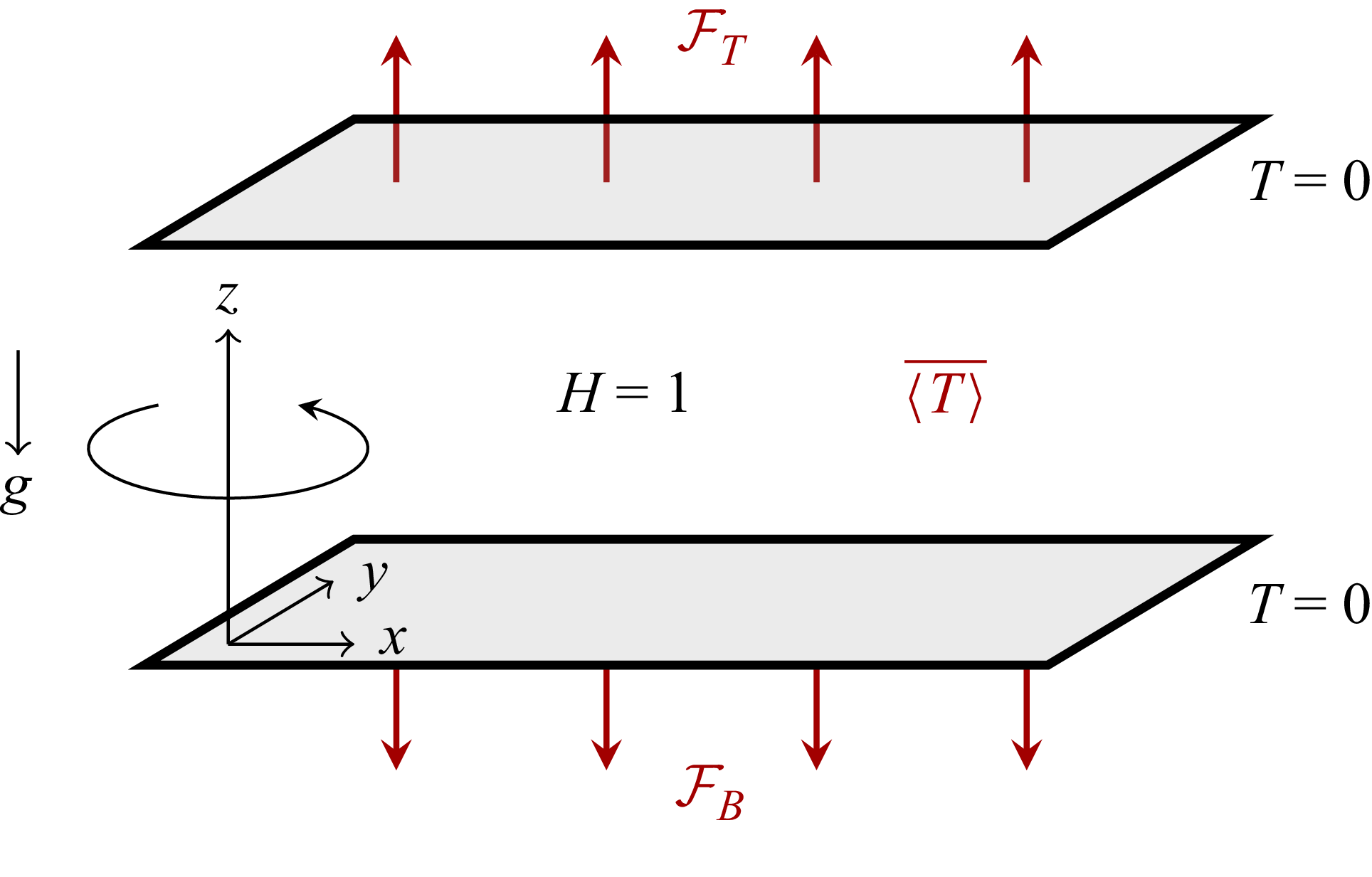


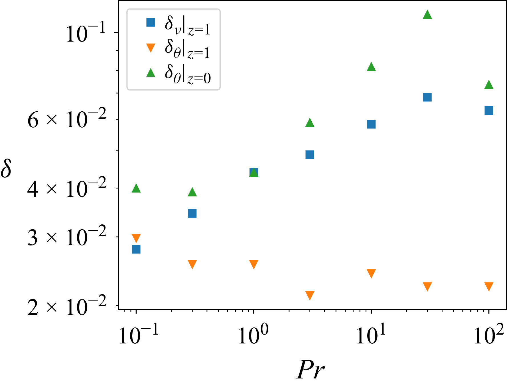


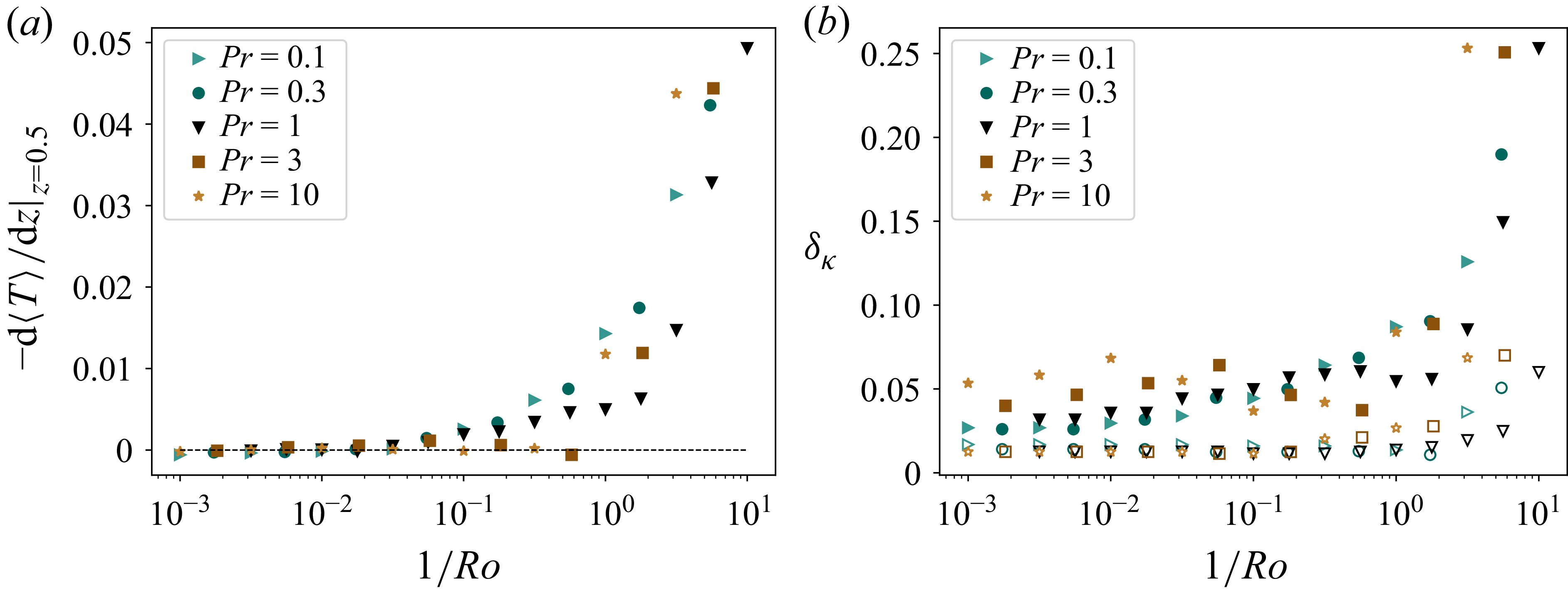


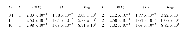


 Open access

