

INTRODUCTION
The Sea of Okhotsk (Fig. 1) is the southernmost sea with a sizable seasonal sea-ice cover in the Northern Hemisphere. Satellite observations (e.g. Gloersen and others, Reference Gloersen1992) show that the initial freezing occurs in the northern part of the sea. The ice cover maximum extent (~1.0 × 10⁶ km2 on average) occurs from the end of February to the beginning of March. The southernmost extent of sea ice reaches the coast of Hokkaido ~44°N. Interannual variability of the maximum ice area is large; ~50–90% of the sea can be covered with ice and the ice typically melts away by June.
Map of the Sea of Okhotsk with bottom topography. The 200- and 3000-m isobars are indicated by thin and thick solid lines, respectively. A box denotes the enlarged portion in Figure 5. White shading indicates sea-ice area (ice concentration ⩾30%) in February averaged for 2003–11; blue shading indicates open ocean area. Ice concentration from AMSR-E is used. Color shadings indicate cumulative ice production in coastal polynyas during winter (December–March) averaged from the 2002/03 to 2009/10 seasons (modified from Nihashi and others, Reference Nihashi, Ohshima and Kimura2012, Reference Nihashi, Ohshima and Saitoh2017). The amount is indicated by the bar scale.
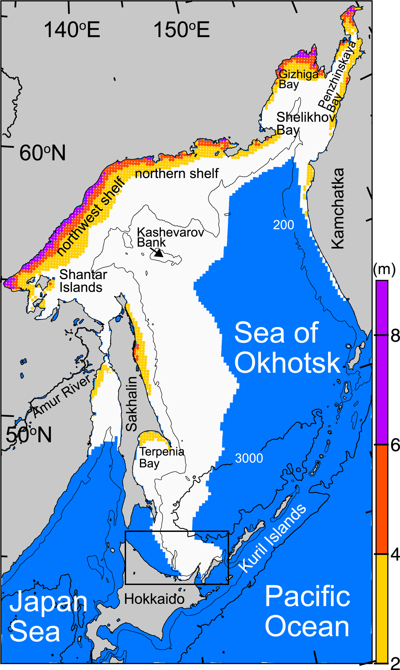
Freezing, transport and melting of sea ice cause a redistribution of heat, salt/fresh water and nutrients. In the Sea of Okhotsk, this process has been suggested to play an important role in the meridional ocean circulation and accordingly the climate and biogeochemical systems of the Sea of Okhotsk and the North Pacific regions. A coastal polynya formed in the northwest shelf region (Fig. 1) is the largest ice production area in the Northern Hemisphere (Ohshima and others, Reference Ohshima, Nihashi and Iwamoto2016). Additionally, a large amount of brine rejection associated with the active freezing forms cold and saline dense water (Shcherbina and others, Reference Shcherbina, Talley and Rudnick2003). This dense water is thought to be the main source for ventilation of the North Pacific Intermediate Water (NPIW; Talley and others, Reference Talley1991; Warner and others, Reference Warner, Bullister, Wisegarver and Gammon1996). In this way, the sea-ice production in coastal polynyas in the Sea of Okhotsk drives the overturning in the North Pacific down to intermediate depths (~200–800 m deep). This overturning can contribute to the material cycle and the subsequent biological productivity through the supply of nutrients such as iron (Nishioka and others, Reference Nishioka2007). Recently, weakening of the overturning due to global warming and associated decrease in ice production has been suggested (Nakanowatari and others, Reference Nakanowatari, Ohshima and Wakatsuchi2007; Ohshima and others, Reference Ohshima, Nakanowatari, Riser, Volkov and Wakatsuchi2014), thus monitoring of changes in sea-ice area and volume are needed to better understand changes in the region. Sea ice formed in the coastal polynyas is advected to the south by the prevailing winds and the East Sakhalin Current (Kimura and Wakatsuchi, Reference Kimura and Wakatsuchi2000; Simizu and others, Reference Simizu, Ohshima, Ono, Fukamachi and Mizuta2014). This leads to a transport of negative heat and fresh water from the north to the south by ice (Ohshima and others, Reference Ohshima, Watanabe and Nihashi2003; Nihashi and others, Reference Nihashi, Ohshima and Kimura2012). Furthermore, sea ice also transports nutrients that affect the primary production in the south (Kanna and others, Reference Kanna, Toyota and Nishioka2014).
Sea-ice volume is an important parameter for understanding the redistribution processes of heat, salt/fresh water, and nutrients by sea ice (Kwok and Rothrock, Reference Kwok and Rothrock1999; Nihashi and others, Reference Nihashi, Ohshima and Kimura2012; Haumann and others, Reference Haumann, Gruber, Münnich, Frenger and Kern2016). Knowledge of the ice volume is also crucial to evaluate the impact of global warming on sea ice. The ice volume is determined by the area and thickness. The ice area has been monitored by passive microwave satellite observations for >30 years, and a decrease trend of −11.9 ± 3.3% decade–1 was shown in the Sea of Okhotsk (Cavalieri and Parkinson, Reference Cavalieri and Parkinson2012). On the other hand, the ice thickness over a broad area has been hard to monitor from both in situ and satellite observations. Thus, until now the ice volume and its trend have been unknown in the Sea of Okhotsk.
At the southernmost area along the Hokkaido coast, measurements of ice draft (ice thickness below the sea surface) had been made by moored ice-profiling sonar (IPS) observations (Fukamachi and others, Reference Fukamachi2003, Reference Fukamachi2006). The ice draft averaged over 1999–2000 is 0.6 m; the annual mean draft ranges between 0.49 and 0.72 m (Fukamachi and others, Reference Fukamachi2006). Similar IPS observations had been conducted near Sakhalin; the ice draft averaged over 2002/03 is 1.05 m (Fukamachi and others, Reference Fukamachi2009). Since a coastal polynya is formed at this site, the ice draft can be separated into distinct periods of thin and thick ice. The ice draft averaged over these thin and thick periods are 0.17 m and 1.95 m, respectively. The thin ice corresponds to the coastal polynya period, while the thick ice is due to drifting of heavily deformed pack ice formed in the north. Near Hokkaido, in situ sea-ice monitoring has been conducted every February by the icebreaker Soya, a patrol vessel of the Japan Coast Guard. Ice thickness was measured from the ship by video and visual observations. The video observations revealed that thickness of undeformed (level) ice averaged over 1991–2000 is 0.33 m (Toyota and others, Reference Toyota, Kawamura, Ohshima, Shimoda and Wakatsuchi2004). Interannual variability of the thickness is large; annual mean thickness of level ice for the above period ranges between 0.19 and 0.55 m. From a comparison with the ice draft measured using moored IPS near Hokkaido (Fukamachi and others, Reference Fukamachi2003), the ice thickness measured by video observation is validated (Toyota and others, Reference Toyota, Kawamura, Ohshima, Shimoda and Wakatsuchi2004). The visual observation revealed that ice thickness averaged over 2003–05 is 111 cm (Toyota and others, Reference Toyota, Takatsuji, Tateyama, Naoki and Ohshima2007), with the primary difference from the video observations being due to the fact that the visual observations included deformed (ridged) ice. Ice-thickness measurements by Electromagnetic Induction Instrument (EM) aboard the icebreaker Soya have been conducted since 2004 (Tateyama and others, Reference Tateyama2006), and the ice thickness was validated from comparisons with that measured by the drill-hole observations within the accuracy of ~10% of the thickness (Uto and others, Reference Uto, Toyota, Shimoda, Tateyama and Shirasawa2006; Toyota and others, Reference Toyota, Nakamura, Uto, Ohshima and Ebuchi2009).
Ice thickness estimation based on satellite observation has been also attempted in the Sea of Okhotsk. Ice thickness was estimated from a radar backscatter image near Hokkaido acquired by synthetic aperture radar (SAR) based on comparisons with ice thickness observed aboard the icebreaker Soya (Nakamura and others, Reference Nakamura2006). Toyota and others (Reference Toyota, Ono, Cho and Ohshima2011) showed ice thickness distributions of the southern Sea of Okhotsk during 2007–09 based on an empirical relationship between the SAR backscatter and ice thickness (surface roughness). The annual mean ice thickness was shown to range between 0.33 and 0.42 m. From a numerical model, ice thickness distributions over the entire Sea of Okhotsk have been simulated (Watanabe and others, Reference Watanabe, Ikeda and Wakatsuchi2004). The model results showed that the ice is thick (~3.5 m) at the southern end of the Shantar Islands.
The Geoscience Laser Altimeter System (GLAS) instrument on the Ice, Cloud and land Elevation Satellite (ICESat) was launched in January 2003, and operated until October 2009. One of two channels of GLAS (at 1064 nm) is used for surface altimetry measurement (Zwally and others, Reference Zwally2002). The footprint size of the laser is ~70 m and the measurement interval is ~170 m along the track. Retrieval of sea-ice freeboard (height of the ice plus snow surface above sea level) has been achieved from the surface elevation measurements by ICESat (Kwok and others, Reference Kwok, Zwally and Yi2004, Reference Kwok, Cunningham, Zwally and Yi2006, Reference Kwok, Cunningham, Zwally and Yi2007; Forsberg and Skourup, Reference Forsberg and Skourup2005; Markus and others, Reference Markus2011).
In the Arctic Ocean, which is predominantly covered by relatively thick multi-year ice, basin-scale ice thickness distribution was estimated based on ICESat-derived freeboard (Kwok and others, Reference Kwok2009). They also showed that ice drafts from ICESat and moored IPSs are consistent within 0.5 m in the Chukchi and Beaufort seas. Ice thickness estimation using ICESat data in the Arctic Ocean has also been conducted by Kurtz and others (Reference Kurtz2009). Zwally and others (Reference Zwally, Yi, Kwok and Zhao2008) and Kern and Spreen (Reference Kern and Spreen2015) had estimated sea-ice thickness from ICESat-derived freeboard in the Weddell Sea, Southern Ocean, where relatively thick ice exists. Kurtz and Markus (Reference Kurtz and Markus2012) estimated sea-ice thickness from ICESat-derived freeboard over the entire Southern Ocean, which is a typical seasonal ice zone similar to the Sea of Okhotsk (the ice thickness was found to be thinner than that in the Arctic Ocean). The objective of this study is to show the retrieval of the sea-ice thickness distribution and volume over the entire Sea of Okhotsk based on ICESat data.
METHODS AND DATA
A schematic illustration for the ice thickness estimation is shown in Figure 2. Total thickness of the sea ice above and below the water level (h i) can be calculated from ICESat-derived freeboard (h f) and snow depth (h s) under the assumption of hydrostatic balance, as follows:
 $$h_i = \displaystyle{{\rho _s - \rho _w} \over {\rho _w - \rho _i}}h_s + \displaystyle{{\rho _w} \over {\rho _w - \rho _i}}h_f.$$
From ice core observations (Toyota and others, Reference Toyota, Takatsuji, Tateyama, Naoki and Ohshima2007), snow and ice densities are assumed to be ρ s = 225 kg m−3 and and ρ i = 888 kg m−3, respectively. Sea-water density is assumed to be ρ w = 1026 kg m−3 from CTD observations (Ohshima and others, Reference Ohshima2001). Based on a relationship between ice thickness and snow depth obtained from in situ measurements (Toyota and others, Reference Toyota, Takatsuji, Tateyama, Naoki and Ohshima2007), h s is given by,
 $$h_s = 0.{\rm 1}h_i.$$
The estimation of h i highly depends on the ρ s, ρ i and h s values. Errors in the h i estimation caused by uncertainty of these parameters are discussed in the summary and discussions section.
In this study, h f is estimated from surface elevation measured by ICESat (h obs; Zwally and others, Reference Zwally2003), following a method by Kurtz and Markus (Reference Kurtz and Markus2012). Filtering of the data are first done since the h obs value is significantly affected by atmospheric scattering due to cloud and blowing snow. The biased h obs data are removed using instrument and waveform-derived parameters that are provided along with the h obs data. To obtain h f, the local sea surface height (h ssh) is subtracted from h obs. The local sea surface height determined by geoid, tides and atmospheric pressure variations (h est) is first estimated, and subtracted from the h obs data. By using the h obs and h est values, h f is given by
 $$h_f = h_{obs} - h_{est} - h_{tp},$$
where h tp is the sea surface tie point. The h tp value is taken to be the average of the lowest three values of h obs−h est that are within ±12.5 km along-track spatial distance from each measurement.
Schematics of sea-ice for estimation of total thickness of ice above and below the water level (h i) from ICESat-derived freeboard (h f). Here, h s is snow depth and h tot (=h s + h i) is total ice thickness including snow depth.
RESULTS
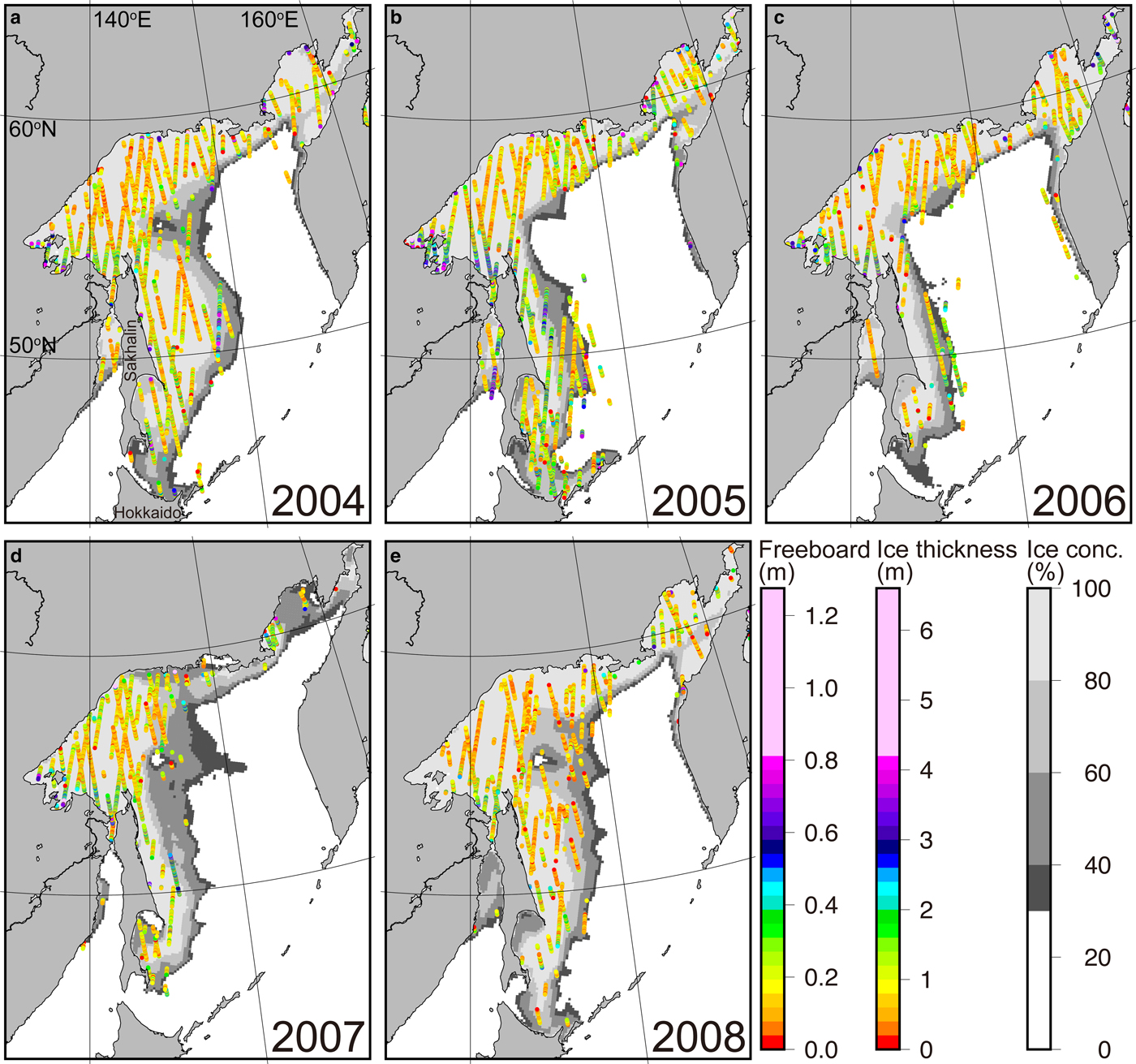
ICESat-derived h f in the Sea of Okhotsk is shown in Figure 3 and the annual and monthly mean h f are shown in Table 1. The data obtained from late-February to mid-March were used, except in 2007 when the data obtained from mid-March to mid-April were used. These periods are determined by the original ICESat collection periods (Zwally and others, Reference Zwally2003). In this study, all available spring ICESat data in the Sea of Okhotsk were used. The number of data points used indicates that the annual mean value is mainly determined by the data in March (Table 1). Sea-ice concentration derived from the Advanced Microwave Scanning Radiometer for EOS (AMSR-E) on the Aqua satellite averaged for February–March (March–April in 2007) is also shown in Figure 3. These periods correspond to the timing of the maximum ice extent. Daily mean ice concentration by Cavalieri and others (Reference Cavalieri, Markus and Comiso2004) were used. The ice concentration data are mapped onto a NSIDC polar stereographic grid at a spatial resolution of ~12.5 km. Sea-ice area (ice area excluding open water fraction) is also shown in Table 1. In this study, the ice edge is defined as the 30% ice concentration contour following Nihashi and others (Reference Nihashi, Ohshima and Kimura2012). Interannual variability of the ice area is large; the largest area occurred in 2004 while the area in 2006 and 2007 was relatively small (Fig. 3). The climatology of h f averaged over the entire period of 2004–08 is 18.3 cm (Table 1).
ICESat-derived freeboard (h f) and total ice thickness (h tot; color) superimposed on AMSR-E derived ice concentration (gray shadings) averaged for February–March (March–April in 2007), when the ICESat data was acquired. In 2004, 2007 and 2008, the Kashevarov Bank polynya, which is a sensible heat polynya (Polyakov and Martin, Reference Polyakov and Martin2000), formed at the Kashevarov Bank region (Fig. 1).
Frequency histograms of total ice thickness (h tot) derived from ICESat. The histogram bin size is 10 cm. n indicates the total number of data points.

Summary of statistics of sea-ice parameters

Here N is number of ICESat data points. The terms h f and h tot indicate freeboard and total ice thickness derived from ICESat data, respectively. For h f and h tot, those averaged over the entire sea-ice zone with spatial Std dev. are shown. For h tot, the modal values are also shown. The term S i indicates net sea-ice area which is given by excluding the open water fraction. For calculating S i, ice concentration derived from AMSR-E data are used. The term V i indicates sea-ice volume obtained from the ICESat h tot and AMSR-E ice concentration. The term Clim. in the bottom row indicates climatology averaged for 5-years of 2004–08 with annual Std dev.
Total sea-ice thickness with snow depth (h tot = h i + h s) which is calculated from Eqns (1) and (2) using h f is also shown in Figure 3. The correspondence between h f and h tot is indicated by the color bars. The annual mean h tot is thinnest in 2008 when the thickness was 77.5 cm (Table 1). The thickest ice was in 2005 when the ice thickness reached 110.4 cm. These reveal that interannual variability of ice thickness is large. No clear relationship between the sea-ice thickness and area is shown (Table 1). The climatological value of h tot averaged over the entire period of 2004–2008 is 95.0 cm. The frequency histogram of h tot is shown in Figure 4. The peak of the histogram (mode) varies between the 50–60 cm thickness bin (2007 and 2008) to the 70–80 cm bin (2005; Table 1).
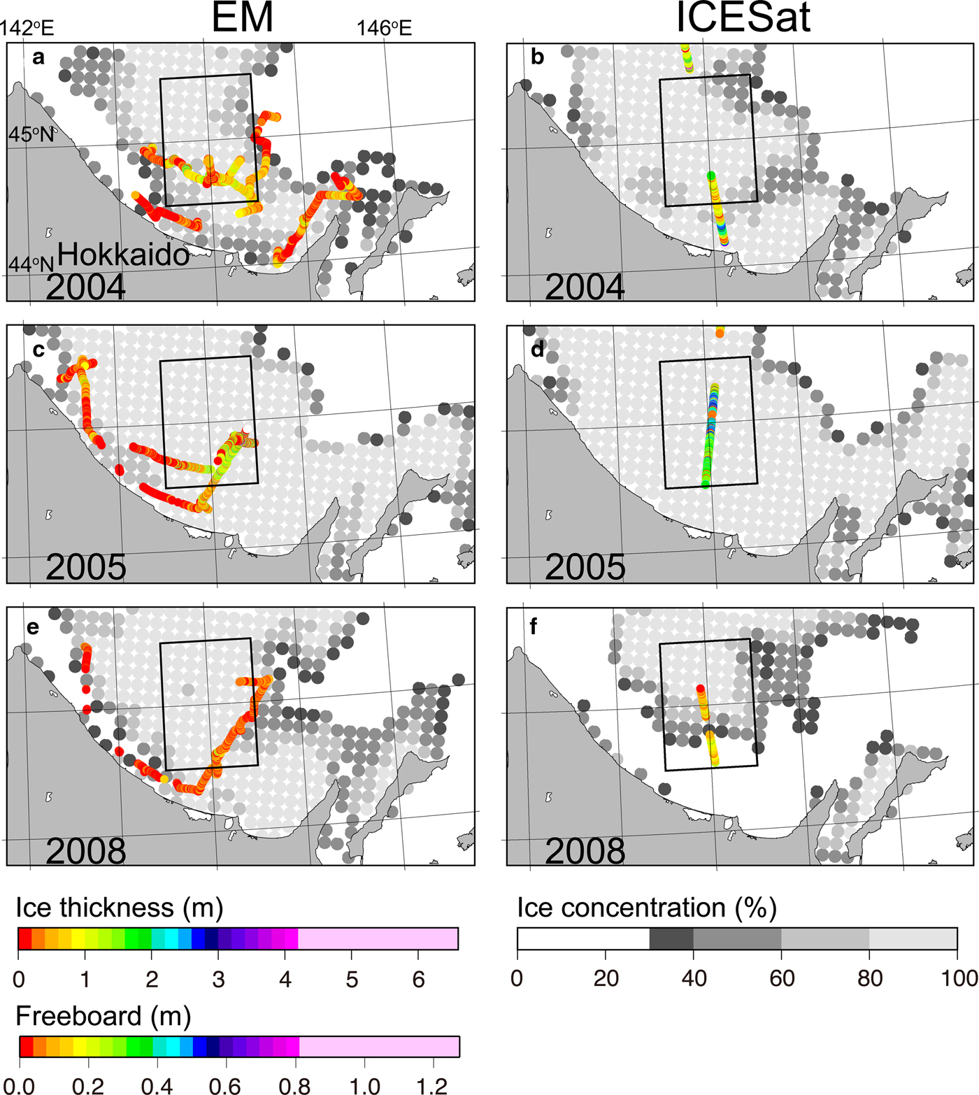
To investigate the quality of the ice thickness retrievals from ICESat data, we compare with thickness observations by EM aboard the icebreaker Soya near Hokkaido. Unfortunately, the ICESat data near Hokkaido is available only for 3 years of 2004, 2005 and 2008 (Fig. 3). The total ice thickness (h tot) from EM measurements is shown in Figure 5a, c, and e with the periods indicated in Table 2. The EM measurements have been carried out in almost the same area and period every year. Close-up maps of the ICESat-derived h tot corresponding to the periods of the EM measurements are shown in Figure 5b, d and f. The periods of the ICESat measurements are also indicated in Table 2. The ICESat measurements in 2004 and 2008 were carried out ~10 days after the EM measurements while the temporal gap is 3 days in 2005. In 2004, maps of daily ice concentration (not shown) indicate that the ice edge had advanced between the EM and ICESat observations. Since the temporal gap of the measurements is short in 2005, significant differences with the sea-ice area were not seen. In 2008, the ice edge had retreated between the EM and ICESat observations.
(a, c and e) Total ice thickness (h tot) derived from EM measurements onboard the icebreaker ‘Soya’. (b, d and f) Freeboard h f and h tot derived from ICESat measurements. The observation periods are indicated in Table 2. Sea-ice concentration derived from AMSR-E of the corresponding period is indicated by gray shadings. A box denotes the analysis area for Figure 6.
The periods of EM observations aboard the icebreaker ‘Soya’ near Hokkaido and date of ICESat measurements in the area

The EM and ICESat-derived h tot are compared by averaging them within an analysis area indicated by a box in Figure 5, this was done because the temporal gap between EM and ICESat data are not small and their footprint size is largely different (10 m vs 70 m). The areas close to Hokkaido, where the effects of convergent ice motion and land contamination are expected to be relatively large, are excluded from the analysis area. The averaged h tot with spatial Std dev. are shown in Figure 6. The interannual variability of the averaged h tot derived from EM and ICESat data roughly corresponds with each other. In 2004, the averaged h tot derived from EM and ICESat data are 87.5 ± 53.4 cm and 84.2 ± 35.7 cm, respectively. The mode of h tot derived from the EM and ICESat data are 60–70 cm bin and 70–80 cm bin, respectively. In that year, the average and modal values are close. In 2005, the averaged h tot derived from EM data are 107.6 ± 81.3 cm, while that from ICESat data are 181.5 ± 69.9 cm. The mode of the ICESat-derived h tot is 160–170 cm, and it is close to the average value. However, the mode of the EM derived h tot is 0–10 cm bin. This indicates that thin ice was dominant around the ship because the EM, whose footprint size is ~10 m, measures ice thickness at the side of the ship. On the other hand, visual observations, in which sea ice is observed in the viewing range of ~1 km, reveal that thicker ice which exceeds continuous ice breaking capability of the ship (>1 m) was prominent. The thin modal value of h tot derived from EM data (0–10 cm bin) indicates that the ship tended to look for thin ice area where the ship can break ice easily and continuously. Even so, the averaged h tot in 2005 from EM data are thickest among the 3 years. In 2008, averaged h tot derived from EM and ICESat data are 45.4 ± 39.6 cm and 70.6 ± 29.8 cm, respectively. The modal values of h tot derived from EM and ICESat data are the 40–50 cm and 60–70 cm bins, respectively.
A scatter plot of total ice thickness (h tot) derived from EM and ICESat data. The ice thickness was averaged over the analysis area shown in Figure 5. Error bars indicate the spatial standard deviations of h tot.

A strict comparison of h tot cannot be made from Figure 6, because data of only 3 years is available and the temporal gap between EM and ICESat data reaches nearly 10 days (Table 2). In the Sea of Okhotsk, sea ice formed in the northern coastal polynyas is advected to the south by the prevailing winds and the East Sakhalin Current, and finally reaches the coast of Hokkaido (Kimura and Wakatsuchi, Reference Kimura and Wakatsuchi2000; Simizu and others, Reference Simizu, Ohshima, Ono, Fukamachi and Mizuta2014). The comparison area of sea-ice thickness is surrounded by the coast of the Kuril Islands and Hokkaido (Figs 1 and 5). Therefore, the advected sea ice is expected to drift around the analysis area for a certain period, because the sea-ice floes must pass narrow straits of the Kuril Islands to flow out into the Pacific. If the averaged h tot derived from EM data represents that of the year, the relationship of h tot shown in Figure 6 validates the ICESat-derived h tot.
The ICESat-derived h tot (Fig. 3) is interpolated onto a polar stereographic grid at a spatial resolution of ~12.5 km using a Gaussian weighting function. This grid is same as that for the AMSR-E ice concentration data. To reveal the spatial distribution of sea-ice thickness over the entire Sea of Okhotsk for the first time, all data of each year, except for the Japan Sea, was used for the interpolation. In the Southern Ocean, a similar spatial interpolation of ICESat-derived ice thickness was made by Kurtz and Markus (Reference Kurtz and Markus2012), and the influence radius was set at 125 km. In this study, the influence radius was set at 210 km because the spatial distribution of ICESat data are relatively sparse in the Sea of Okhotsk which is located at lower latitude. The spatial distribution of h tot mapped onto the polar stereographic grid is shown in Figure 7. The open ocean is masked as the area where the AMSR-E ice concentration averaged from February to March (from March to April in 2007) is <30%. Ice thickness is relatively thin at the northwest shelf and north shelf regions where coastal polynyas are formed (Nihashi and others, Reference Nihashi, Ohshima, Tamura, Fukamachi and Saitoh2009). On the other hand, ice thickness is relatively thick south of the Shantar Islands. This is considered to be caused by convergent ice motion. Similarly, ice thickness is relatively thick near Hokkaido. Ice thickness is relatively thick also in the Shelikhov and Penzhinskaya Bays. This might be caused by sea-ice deformation due to strong tides in this area (Kowalik and Polyakov, Reference Kowalik and Polyakov1998). The spatial distribution of sea-ice thickness is similar every year, although the thickness is different. For example, the thickness in 2008 is thinnest over almost the entire sea-ice zone. The spatial distribution of ice thickness derived from ICESat data are roughly similar to that from a numerical model (Watanabe and others, Reference Watanabe, Ikeda and Wakatsuchi2004).
ICESat-derived total ice thickness h tot interpolated onto the polar stereographic grid at the 12.5 km spatial resolution. (f) Climatology of h tot averaged for 2004–08. A black line denotes an analysis area along 53°N used in Summary and Discussions. The sea-ice data in the Japan Sea is masked out.

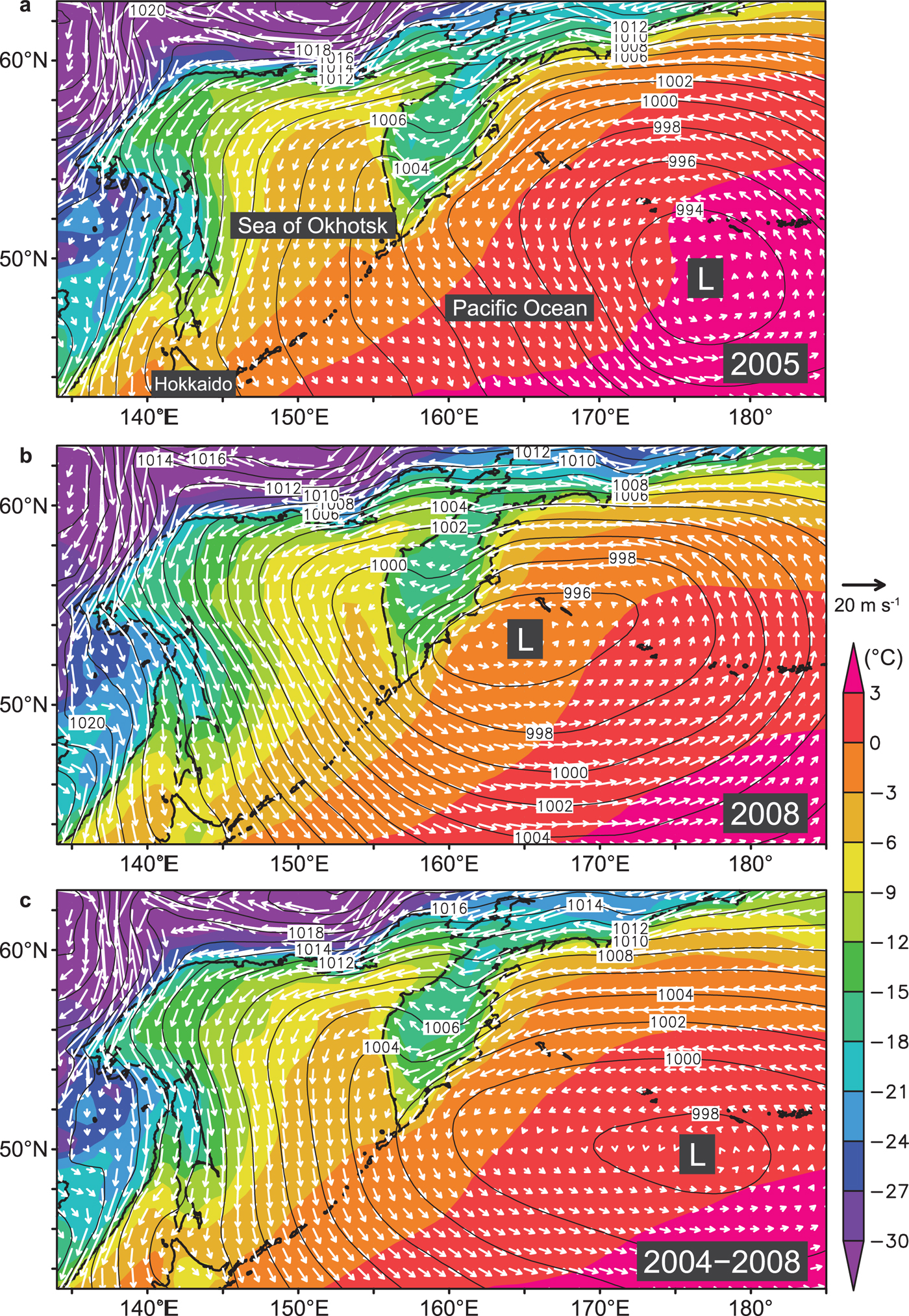
In 2005, when the average h tot is the thickest (Table 1), the position of the Aleutian Low in January was somewhat to the south of its usual location (Fig. 8a and c). This indicates that the westward wind component which leads to convergent ice motion was relatively strong. The thickest ice in 2005 is considered to be caused by deformation of ice due to this anomalous wind. On the other hand, in 2008 when the average total thickness is the thinnest (Table 1), the position of the Aleutian Low in January was somewhat to the northeast of the normal location (Fig. 8b and c). This indicates that the eastward wind component which leads to divergent ice motion was relatively strong. These results indicate that the synoptic scale wind is an important factor causing interannual variability of ice thickness in the Sea of Okhotsk.
(a) Sea-level pressure (solid lines), geostrophic wind (vectors), and air temperature at 2 m (colors), averaged for the sea-ice advance season (January) in 2005. (b) As in (a), but for data in 2008. (c) As in (a), but for data averaged for 2004–08. We used near-surface atmospheric data from the 6-hourly ECMWF interim reanalysis (ERA-Interim) dataset with a spatial resolution of 0.5° × 0.5°.
Sea-ice volume is estimated from AMSE-E derived ice area (concentration) averaged for February–March (March–April in 2007) multiplied by the ICESat-derived h tot (Fig. 7) at each gridpoint. Total ice volume (sum of ice volume over the sea-ice gridpoints) in the Sea of Okhotsk is compared with annual ice production in major coastal polynyas (northwest shelf region, north shelf region, Gizhiga Bay, coastal regions of western Kamchatka and northeastern Sakhalin, and Terpenia Bay; Fig. 1). This ice production is based on heat budget calculation using thin ice thickness derived from AMSR-E (Nihashi and others, Reference Nihashi, Ohshima and Kimura2012). A time series of the ice volume is shown in Figure 9. For comparison, a time series of sea-ice area (Table 1) is superimposed on the figure. Variability of the ice volume roughly corresponds to that presumed from the ice area if the thickness is assumed to be 1 m. However, ice volume in 2008 is relatively small owing to the lowest ice thickness (Table 1). This indicates that ice area cannot be used as a proxy of ice volume. Time series of annual ice production in the major coastal polynyas is also shown in Figure 9. The ice volume and annual ice production estimated from independent data are generally comparable. This also supports validity of the estimations of sea-ice thickness and volume from satellite altimetry data.
Time series of ice volume (black solid line with triangles), ice area (gray solid line with dots) and ice production in major coastal polynyas (gray dashed line with squares) in the Sea of Okhotsk.

SUMMARY AND DISCUSSIONS
In the entire sea-ice zone of the Sea of Okhotsk, the total sea-ice thickness including snow depth (h tot) for 2004–08 was estimated using ICESat-derived freeboard (Fig. 3), and revealed the spatial distribution of thickness for the first time (Fig. 7). The h tot derived from ICESat data roughly corresponded with that derived from EM data near Hokkaido (Fig. 6). The errors in the h tot, which is calculated from Eqns (1) and (2), are mainly caused by the densities of snow (ρ s) and sea-ice (ρ i), snow depth (h s), and ICESat-derived freeboard (h f). In this study, densities of snow and sea ice were assumed to be ρ s = 225 kg m−3 and ρ i = 888 kg m−3, respectively. These values are based on in situ measurements, and variations of ρ s and ρ i were estimated as ± 109 kg m−3 and ± 23 kg m−3, respectively (Toyota and others, Reference Toyota, Takatsuji, Tateyama, Naoki and Ohshima2007). The h tot errors caused by ρ s and ρ i are estimated by using these values. In the winter Arctic Ocean, relatively higher values of ρ s (300–320 kg m−3) are shown (Warren and others, Reference Warren1999). It is noted that the ρ s value (225 ± 109 kg m−3) used in the error estimation covers these relatively higher ρ s values in the Arctic Ocean. The ratio of h tot changed by the perturbation of ρ s and ρ i are ~±5% and ~±10%, respectively. For example, in a case of h tot = 95.0 cm, which is estimated from a mean freeboard h f of 18.3 cm (Table 1), the errors caused by ρ s and ρ i are ~±5 cm and ~±10 cm, respectively. In this study, snow depth h s was assumed to be 10% of the ice thickness h i (Eqn 2) based on in situ measurements (Toyota and others, Reference Toyota, Takatsuji, Tateyama, Naoki and Ohshima2007). From the in situ measurements of snow depth, a regression line of h s = 0.041 h i + 6.070 (cm) was shown in Toyota and others (Reference Toyota, Takatsuji, Tateyama, Naoki and Ohshima2007). However, we did not use this regression line, because a negative h i value is calculated when the h f value is small (h f < ~5 cm). It is noted that h tot estimated from a mean h f of 18.3 cm using this regression line for h s is ~93 cm, and this h tot value is similar to that estimated assuming that h s = 0.1 h i (95 cm; Table 1). When h s is assumed that h s = 0.05 h i based on the in situ measurements by Toyota and others (Reference Toyota, Takatsuji, Tateyama, Naoki and Ohshima2007), h tot is estimated to be ~45% thicker than the baseline case in which h s was assumed that h s = 0.1 h i. On the other hand, h tot is estimated to be ~15% thinner than the baseline case when h s is assumed that h s = 0.15 h i. The uncertainty of h f has previously been shown to be 1.8 cm (Markus and others, Reference Markus2011). This causes the h tot error of ~9.3 cm. These estimations indicate that the h tot errors owing to ρ s, ρ i, h s and h f do not affect the validation of the ice thickness estimation shown in Figure 6.
Interannual variability of h tot averaged over the entire sea-ice zone was shown to be large. The minimum value is 77.5 cm in 2008, while the maximum value is 110.4 cm in 2005 (Table 1). A frequency histogram of h tot (Fig. 4) revealed that the mode varies from 50–60 cm thickness bin in 2007 and 2008 to 70–80 cm bin in 2005 (Table 1). These thickness values are much higher than the maximum thickness of thermodynamically grown pack ice without deformation observed in the Antarctic Ocean (0.3–0.4 m; e.g. Allison and Worby, Reference Allison and Worby1994; Jeffries and others, Reference Jeffries, Worby, Morris and Weeks1997; Wadhams and others, Reference Wadhams, Lange and Ackley1987). This indicates that deformed ice is prominent over the entire Okhotsk sea-ice zone as suggested from in situ observations of sea ice in the southernmost part of the sea (Toyota and others, Reference Toyota, Kawamura, Ohshima, Shimoda and Wakatsuchi2004, Reference Toyota, Takatsuji, Tateyama, Naoki and Ohshima2007). Furthermore, the large tails of the distributions (Fig. 4) and mean thickness values of >~80 cm (Table 1) indicate that the deformed ice affects ice volume in the Sea of Okhotsk.
Ice volume in the Sea of Okhotsk was estimated from ICESat-derived h tot and AMSR-E derived ice concentration (Fig. 9). Sea-ice area has been used for a proxy of ice volume in the Sea of Okhotsk when there is no ice thickness information (e.g., Nihashi and others, Reference Nihashi, Ohshima and Nakasato2011). However, the results of this study indicated that ice area cannot always represent the ice volume (Fig. 9), as in the case of 2008 when the average ice thickness was thin (Table 1). The ice volume estimated in this study was shown to roughly correspond to ice production in major coastal polynyas estimated based on heat flux calculations (Fig. 9). This supports the validity of ice thickness and volume estimation based on ICESat data.
In the Sea of Okhotsk, sea ice formed in the northern coastal polynyas is advected to the south by the prevailing northerly winds and the southward East Sakhalin Current. This indicates a transportation of negative heat, fresh water and nutrients to the south by sea ice. Simizu and others (Reference Simizu, Ohshima, Ono, Fukamachi and Mizuta2014) estimated the southward ice-volume transport using sea-ice drift based on the moored Acoustic Doppler Current Profiler (ADCP), an ocean model simulation, objective analysis data of the wind, and satellite sea-ice data. Since there was no ice thickness information, they simply assumed a uniform ice thickness of 1 m. The cumulative southward ice transport per winter, which crosses a line along 53°N (Fig. 1), was estimated to be 3.0 × 10¹¹ m3. From the climatology of ICESat-derived h tot of this study (Fig. 7f), h tot averaged on the line is estimated to be ~85 cm. Furthermore, h tot averaged over the entire Sea of Okhotsk is 95 cm (Table 1). These indicate that the assumption of ice thickness of 1 m in Simizu and others (Reference Simizu, Ohshima, Ono, Fukamachi and Mizuta2014) was almost appropriate. When the ICESat-derived h tot (=85 cm) is adopted to the estimation by Simizu and others (Reference Simizu, Ohshima, Ono, Fukamachi and Mizuta2014), the cumulative southward ice transport per winter is estimated to be 2.6 × 10¹¹ m3. This ice transport is comparable with the climatological annual discharge of the Amur River (Fig. 1) of 3.1 × 10¹¹ m3 (Fig. 1; Dai and others, Reference Dai, Qian, Trenberth and Milliman2009).
The primary goal of this study was to reveal the spatial distribution of sea-ice thickness in the Sea of Okhotsk for the first time. In order to understand changes in sea ice associated with climate change, a decadal time series of sea-ice volume is needed. Sea-ice area in the Sea of Okhotsk has been decreasing at a rate of ~12% decade−1 for the last 30 years (Cavalieri and Parkinson, Reference Cavalieri and Parkinson2012). Furthermore, sea-ice production also has been decreasing ~11% for the last 30 years due to warming in autumn at the land area northwest of the Sea of Okhotsk (Kashiwase and others, Reference Kashiwase, Ohshima and Nihashi2014). Creating a decadal-scale record of ice thickness requires merging multiple satellite records. ICESat covers only for the period of 2004–08. In April 2010, a radar altimeter on CryoSat-2 was launched, and ice thickness and volume can be estimated also from this data (e.g. Laxon and others, Reference Laxon2013). By combining the CryoSat-2 data (2010–) with the ICESat data, a time series of ice volume that covers >10 years can be obtained. However, the CryoSat-2 data cannot be directly compared with the ICESat data because the observation periods do not overlap. Furthermore, as shown in Table 2 and Figures 5 and 6, a strict comparison of ice thickness between satellite and in situ observations also cannot be made in the Sea of Okhotsk owing to the large temporal gap of the measurements. Therefore, we have not included the CryoSat-2 data in this study, because reliability of the time series of ice volume requires a further in-depth study. In 2018, ICESat-2, which is a successor to ICESat used in this study, is planned for launch. This data can be compared with the CryoSat-2 data. In the future, analysis combining these satellite-derived ice thickness would be important for discussing the longer term variability of ice volume in the Sea of Okhotsk where the strong influence of global warming on sea ice has been implicated.
ACKNOWLEDGEMENTS
The ICESat data were obtained from the NASA National Snow and Ice Data Center (NSIDC) Distributed Active Archive Center. The AMSR-E data were provided by the NSIDC. Comments from the editor and two reviewers were very helpful. This work was supported by Grant-in-Aids for Scientific Research (17K00530) of the Japanese Ministry of Education, Culture, Sports, Science and Technology (MEXT).


 Open access