


1. Introduction
Thermal convection – the buoyancy-driven transport of mass and heat – is an omnipresent fluid flow process in nature, occurring not just in geophysical systems like clusters of clouds over the ocean (Mapes & Houze Reference Mapes and Houze1993) or the Earth’s mantle (Chillà & Schumacher Reference Chillà and Schumacher2012), but also on other planets such as the storms on Jupiter (Young & Read Reference Young and Read2017) and Saturn (García-Melendo, Huseo & Sánchez-Lavega Reference García-Melendo, Hueso and Sánchez-Lavega2013) or stars like in the Sun’s solar convection zone (Schumacher & Sreenivasan Reference Schumacher and Sreenivasan2020). Understanding this process is thus vital to comprehending geo- and astrophysical flows.
Rayleigh–Bénard convection can be seen as the paradigm of such, containing all essential ingredients and permitting the investigation of even complex convection phenomena like pattern formation in detail. There, fluid is confined between two parallel, horizontally extended plates while being heated from below and cooled from above. When interacting with gravity, an interplay between buoyant and viscous forces occurs which is quantified by the Rayleigh number
 $Ra$
. Once thermal driving gets strong enough to destabilise the fluid layer – marked by passing the critical Rayleigh number
$Ra$
. Once thermal driving gets strong enough to destabilise the fluid layer – marked by passing the critical Rayleigh number
 $Ra_{c}$
– instabilities start growing and convection sets in (Rayleigh Reference Rayleigh1916).
$Ra_{c}$
– instabilities start growing and convection sets in (Rayleigh Reference Rayleigh1916).
By virtue of rapid improvements in computational power, it only became possible in recent years to numerically study large-scale pattern formation for extended domains due to the strong scale separation towards the small Kolmogorov or Batchelor scales (Scheel, Emran & Schumacher Reference Scheel, Emran and Schumacher2013). Extended fluid domains, i.e. domains possessing a (horizontal) aspect ratio
 ${\Gamma }=L/H \gg 1$
where
${\Gamma }=L/H \gg 1$
where
 $L$
and
$L$
and
 $H$
are the horizontal and vertical extent, respectively, are vital for understanding natural systems. Since the influence of lateral boundaries decreases with
$H$
are the horizontal and vertical extent, respectively, are vital for understanding natural systems. Since the influence of lateral boundaries decreases with
 $\textit {O} ({\Gamma }^{-2} )$
(Manneville Reference Manneville2006; Cross & Greenside Reference Cross and Greenside2009; Koschmieder 2009), it is typically assumed that
$\textit {O} ({\Gamma }^{-2} )$
(Manneville Reference Manneville2006; Cross & Greenside Reference Cross and Greenside2009; Koschmieder 2009), it is typically assumed that
 ${\Gamma } \gtrsim 20$
lets this impact practically vanish and thus approximates real-life scenarios fairly well (Koschmieder 2009; Stevens et al. Reference Stevens, Blass, Zhu, Verzicco and Lohse2018; Krug, Lohse & Stevens Reference Krug, Lohse and Stevens2020).
${\Gamma } \gtrsim 20$
lets this impact practically vanish and thus approximates real-life scenarios fairly well (Koschmieder 2009; Stevens et al. Reference Stevens, Blass, Zhu, Verzicco and Lohse2018; Krug, Lohse & Stevens Reference Krug, Lohse and Stevens2020).
Traditionally, the heating and cooling of the fluid has been achieved in two ways: either applying (two different) constant temperatures (i.e. Dirichlet type thermal boundary condition) or a constant heat flux (i.e. Neumann type). Previous studies have found that these thermal boundary conditions govern the pattern formation process, leading to either turbulent superstructures – an arrangement of large-scale convection rolls and cells of size
 $\varLambda \sim \textit {O} ( H )$
– in the Dirichlet case (Pandey, Scheel & Schumacher Reference Pandey, Scheel and Schumacher2018; Stevens et al. Reference Stevens, Blass, Zhu, Verzicco and Lohse2018) or a pair of supergranules – two pairs of larger-scale convection rolls
$\varLambda \sim \textit {O} ( H )$
– in the Dirichlet case (Pandey, Scheel & Schumacher Reference Pandey, Scheel and Schumacher2018; Stevens et al. Reference Stevens, Blass, Zhu, Verzicco and Lohse2018) or a pair of supergranules – two pairs of larger-scale convection rolls
 $\varLambda \sim {\Gamma } H \gg \textit {O} ( H )$
that eventually span across the entire domain – in the Neumann case (Vieweg et al. Reference Vieweg, Scheel and Schumacher2021, Reference Vieweg, Scheel, Stepanov and Schumacher2022, Reference Vieweg, Klünker, Schumacher and Padberg-Gehle2024; Vieweg, Reference Vieweg2024a
). Interestingly, both kinds of these turbulent long-living large-scale flow structures (Vieweg Reference Vieweg2023) are reminiscent of the respective critical pattern present at the onset of convection (Rayleigh Reference Rayleigh1916; Pellew & Southwell Reference Pellew and Southwell1940; Hurle, Jakeman & Pike Reference Hurle, Jakeman and Pike1967).
$\varLambda \sim {\Gamma } H \gg \textit {O} ( H )$
that eventually span across the entire domain – in the Neumann case (Vieweg et al. Reference Vieweg, Scheel and Schumacher2021, Reference Vieweg, Scheel, Stepanov and Schumacher2022, Reference Vieweg, Klünker, Schumacher and Padberg-Gehle2024; Vieweg, Reference Vieweg2024a
). Interestingly, both kinds of these turbulent long-living large-scale flow structures (Vieweg Reference Vieweg2023) are reminiscent of the respective critical pattern present at the onset of convection (Rayleigh Reference Rayleigh1916; Pellew & Southwell Reference Pellew and Southwell1940; Hurle, Jakeman & Pike Reference Hurle, Jakeman and Pike1967).
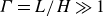
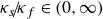
Fundamental configuration. In Rayleigh–Bénard convection, (a) a layer of fluid is confined between a heated bottom and a cooled top plane, respectively. While these planes are typically also the limits of the numerical domain, (b) this study includes the (otherwise omitted) adjacent plates together with the coupled or conjugate heat transfer (CHT) across the two solid–fluid interfaces. The location of different temperatures is defined on the right while only
 $T_h$
and
$T_h$
and
 $T_c$
are controlled – other temperatures manifest dynamically. In this study,
$T_c$
are controlled – other temperatures manifest dynamically. In this study,
 $\kappa _{st} = \kappa _{sb} = \kappa _{s}$
and
$\kappa _{st} = \kappa _{sb} = \kappa _{s}$
and
 ${\Gamma }_{st} = {{\Gamma }_{sb}} = {\Gamma _s}$
.
${\Gamma }_{st} = {{\Gamma }_{sb}} = {\Gamma _s}$
.
These two conditions, however, represent mathematically idealised scenarios, which are illustrated in figure 1(a). In fact, they omit the vertically adjacent matter or solid that confines and, thus, influences the fluid. Using a conjugate heat transfer (CHT) set-up addresses the problem more holistically by modelling these plates as solid thermal conductors such that not only the heat transfer in the fluid, but also in the adjacent solids as well as their solid–fluid interaction is considered (Perelman Reference Perelman1961). Here, as illustrated in figure 1(b), (external) thermal boundary conditions are applied as constant temperatures
 $T_h$
and
$T_h$
and
 $T_c$
at the very bottom and top of the solid plates of relative thickness or vertical aspect ratio
$T_c$
at the very bottom and top of the solid plates of relative thickness or vertical aspect ratio
 ${\Gamma _s}=H_s/H$
, respectively. This causes a temperature gradient within the solid plates before reaching the (internal) thermal boundary conditions at the solid–fluid interfaces – offering the, based on system dynamics, dynamically manifesting temperatures
${\Gamma _s}=H_s/H$
, respectively. This causes a temperature gradient within the solid plates before reaching the (internal) thermal boundary conditions at the solid–fluid interfaces – offering the, based on system dynamics, dynamically manifesting temperatures
 $T_b$
and
$T_b$
and
 $T_t$
– where both the temperature and heat flux are coupled between the different subdomains.
$T_t$
– where both the temperature and heat flux are coupled between the different subdomains.
The ratio of thermal diffusivities between the solids and the fluid,
 $\kappa _s \! / \! \kappa _f$
, plays an integral role in governing the aforementioned pattern formation process as the Neumann case is represented by
$\kappa _s \! / \! \kappa _f$
, plays an integral role in governing the aforementioned pattern formation process as the Neumann case is represented by
 $\kappa _s \! / \! \kappa _f \rightarrow 0$
whereas the Dirichlet case corresponds to
$\kappa _s \! / \! \kappa _f \rightarrow 0$
whereas the Dirichlet case corresponds to
 $\kappa _s \! / \! \kappa _f \rightarrow \infty$
. While previous studies in large aspect ratios (Pandey et al. Reference Pandey, Scheel and Schumacher2018; Vieweg et al. Reference Vieweg, Scheel and Schumacher2021, Reference Vieweg, Schneide, Padberg-Gehle and Schumacher2021a
, Reference Vieweg, Scheel, Stepanov and Schumacher2022; Schneide et al. Reference Schneide, Vieweg, Schumacher and Padberg-Gehle2022, 2024, 2025; Vieweg Reference Vieweg2023, Reference Vieweg2024a
) have only been focusing on these extreme ends, natural systems always are located somewhere in between. Although some studies of finite
$\kappa _s \! / \! \kappa _f \rightarrow \infty$
. While previous studies in large aspect ratios (Pandey et al. Reference Pandey, Scheel and Schumacher2018; Vieweg et al. Reference Vieweg, Scheel and Schumacher2021, Reference Vieweg, Schneide, Padberg-Gehle and Schumacher2021a
, Reference Vieweg, Scheel, Stepanov and Schumacher2022; Schneide et al. Reference Schneide, Vieweg, Schumacher and Padberg-Gehle2022, 2024, 2025; Vieweg Reference Vieweg2023, Reference Vieweg2024a
) have only been focusing on these extreme ends, natural systems always are located somewhere in between. Although some studies of finite
 $\kappa _s \! / \! \kappa _f$
have already analysed heat transfer in a CHT set-up experimentally (Vasil’ev et al. Reference Vasil’ev, Kolesnichenko, Mamykin, Frick, Khalilov, Rogozhekin and Pakholkov2015) or for cylindrical cells of small aspect ratios
$\kappa _s \! / \! \kappa _f$
have already analysed heat transfer in a CHT set-up experimentally (Vasil’ev et al. Reference Vasil’ev, Kolesnichenko, Mamykin, Frick, Khalilov, Rogozhekin and Pakholkov2015) or for cylindrical cells of small aspect ratios
 ${\Gamma }=1/2$
(Verzicco Reference Verzicco2002, Reference Verzicco2004; Foroozani, Krasnov & Schumacher Reference Foroozani, Krasnov and Schumacher2021) and others have contrasted the difference in heat transport between the Dirichlet and Neumann cases in small cells (Verzicco & Sreenivasan Reference Verzicco and Sreenivasan2008; Johnston & Doering Reference Johnston and Doering2009), the pattern formation process has not yet been investigated. Since both turbulent superstructures (Krug et al. Reference Krug, Lohse and Stevens2020) and supergranules (Vieweg, Scheel & Schumacher Reference Vieweg, Scheel and Schumacher2021) are of crucial importance for the induced heat transfer across the fluid layer, a detailed understanding of pattern formation is indispensable. Moreover, the ratio of thermophysical properties between the solid and fluid is crucial beyond our focus on pattern formation aspects, e.g. for the turbulent heat transfer across the fluid layer. This holds particularly for laboratory experiments at very large Rayleigh numbers of
${\Gamma }=1/2$
(Verzicco Reference Verzicco2002, Reference Verzicco2004; Foroozani, Krasnov & Schumacher Reference Foroozani, Krasnov and Schumacher2021) and others have contrasted the difference in heat transport between the Dirichlet and Neumann cases in small cells (Verzicco & Sreenivasan Reference Verzicco and Sreenivasan2008; Johnston & Doering Reference Johnston and Doering2009), the pattern formation process has not yet been investigated. Since both turbulent superstructures (Krug et al. Reference Krug, Lohse and Stevens2020) and supergranules (Vieweg, Scheel & Schumacher Reference Vieweg, Scheel and Schumacher2021) are of crucial importance for the induced heat transfer across the fluid layer, a detailed understanding of pattern formation is indispensable. Moreover, the ratio of thermophysical properties between the solid and fluid is crucial beyond our focus on pattern formation aspects, e.g. for the turbulent heat transfer across the fluid layer. This holds particularly for laboratory experiments at very large Rayleigh numbers of
 $Ra\gtrsim 10^{12}$
where the enhanced turbulence-induced effective conductivity in the fluid can be close to the one in the plates. This requires corrections in
$Ra\gtrsim 10^{12}$
where the enhanced turbulence-induced effective conductivity in the fluid can be close to the one in the plates. This requires corrections in
 $Nu$
, which have been discussed, for example, by Niemela & Sreenivasan (Reference Niemela and Sreenivasan2006).
$Nu$
, which have been discussed, for example, by Niemela & Sreenivasan (Reference Niemela and Sreenivasan2006).
This study aims to represent natural scenarios of
 $\kappa _s \! / \! \kappa _f \in ( 0, \infty )$
at a large aspect ratio
$\kappa _s \! / \! \kappa _f \in ( 0, \infty )$
at a large aspect ratio
 ${\Gamma }=30$
more accurately by considering the coupled or conjugate heat transfer (CHT) at the solid–fluid interfaces, thus coining the term natural thermal boundary conditions. Comprehending this region is crucial to enhancing our understanding of convection flows and their properties in real-life geo- and astrophysical scenarios. To do so, direct numerical simulations are conducted for two Rayleigh numbers
${\Gamma }=30$
more accurately by considering the coupled or conjugate heat transfer (CHT) at the solid–fluid interfaces, thus coining the term natural thermal boundary conditions. Comprehending this region is crucial to enhancing our understanding of convection flows and their properties in real-life geo- and astrophysical scenarios. To do so, direct numerical simulations are conducted for two Rayleigh numbers
 $Ra=\{10^4,10^5\}$
over an array of different
$Ra=\{10^4,10^5\}$
over an array of different
 $\kappa _s \! / \! \kappa _f$
. As a primary result of this work, we observe pronounced gradual shifts of both the size of flow structures and their induced heat transfer when varying
$\kappa _s \! / \! \kappa _f$
. As a primary result of this work, we observe pronounced gradual shifts of both the size of flow structures and their induced heat transfer when varying
 $\kappa _s \! / \! \kappa _f$
, underlining the importance of long-living large-scale flow structures as an umbrella term for both turbulent superstructures and supergranules. The transition of large-scale flow structures comes with gradual shifts in both the thermal as well as viscous boundary layer thicknesses. This numerical approach is complemented theoretically by a comprehensive linear stability analysis regarding the onset of convection. This analysis confirms the aforementioned transition between flow structures as a gradual shift towards larger critical wavenumbers
$\kappa _s \! / \! \kappa _f$
, underlining the importance of long-living large-scale flow structures as an umbrella term for both turbulent superstructures and supergranules. The transition of large-scale flow structures comes with gradual shifts in both the thermal as well as viscous boundary layer thicknesses. This numerical approach is complemented theoretically by a comprehensive linear stability analysis regarding the onset of convection. This analysis confirms the aforementioned transition between flow structures as a gradual shift towards larger critical wavenumbers
 $k_{c}$
is observed when moving from Neumann to Dirichlet conditions. As the vertical aspect ratio or plate thickness
$k_{c}$
is observed when moving from Neumann to Dirichlet conditions. As the vertical aspect ratio or plate thickness
 $\Gamma _s$
represents an additional free parameter in the CHT set-up, we extend both of our approaches towards a variation of
$\Gamma _s$
represents an additional free parameter in the CHT set-up, we extend both of our approaches towards a variation of
 $\Gamma _s$
and find that thin plates stabilise the layer especially for moderate
$\Gamma _s$
and find that thin plates stabilise the layer especially for moderate
 $\lambda _s \! / \! \lambda _f$
. We remark that this, together with easy-to-handle regression fits, extends the results obtained by Hurle et al. (Reference Hurle, Jakeman and Pike1967) for infinitely thick plates. The present study bridges the gap between classical thermal boundary conditions by incorporating solid subdomains together with the coupled temperatures and heat transfers at the solid–fluid interfaces, allowing us to interpret natural flows in the geo- and astrophysical context more successfully.
$\lambda _s \! / \! \lambda _f$
. We remark that this, together with easy-to-handle regression fits, extends the results obtained by Hurle et al. (Reference Hurle, Jakeman and Pike1967) for infinitely thick plates. The present study bridges the gap between classical thermal boundary conditions by incorporating solid subdomains together with the coupled temperatures and heat transfers at the solid–fluid interfaces, allowing us to interpret natural flows in the geo- and astrophysical context more successfully.
2. Governing equations and numerical method
2.1. Governing equations
We consider an incompressible flow based on the Oberbeck–Boussinesq approximation (Oberbeck Reference Oberbeck1879; Boussinesq Reference Boussinesq1903). This means that all material parameters are constant – except for the mass density, the latter of which varies at first order with temperature when interacting with gravity only. The three-dimensional equations of motion are non-dimensionalised based on the fluid layer height
 $H$
and the temperatures at the bottom and top of this fluid layer,
$H$
and the temperatures at the bottom and top of this fluid layer,
 $T_b$
and
$T_b$
and
 $T_t$
(see also figure 1
b), respectively. We use the spatiotemporal average of these temperature fields to define the characteristic (dimensional) temperature scale
$T_t$
(see also figure 1
b), respectively. We use the spatiotemporal average of these temperature fields to define the characteristic (dimensional) temperature scale
 $\Delta T := \langle T_b - T_t \rangle _{A,t}$
where
$\Delta T := \langle T_b - T_t \rangle _{A,t}$
where
 $A$
denotes the entire horizontal cross-section. Note that this implies a non-dimensionalisation
$A$
denotes the entire horizontal cross-section. Note that this implies a non-dimensionalisation
 $T = \Delta T \, \tilde {T}$
together with the assumption of a resulting non-dimensional temperature difference across the fluid layer of
$T = \Delta T \, \tilde {T}$
together with the assumption of a resulting non-dimensional temperature difference across the fluid layer of
 $\Delta T_N := \langle \tilde {T_b} - \tilde {T_t} \rangle _{A,t} \equiv 1$
. We stress explicitly that we write out the tildes here to clearly distinguish the dimensional
$\Delta T_N := \langle \tilde {T_b} - \tilde {T_t} \rangle _{A,t} \equiv 1$
. We stress explicitly that we write out the tildes here to clearly distinguish the dimensional
 $\Delta T$
and non-dimensional temperature difference
$\Delta T$
and non-dimensional temperature difference
 $\Delta T_N$
but will, from now on, mostly omit such for better readability. By virtue of the free-fall inertia balance, the free-fall velocity
$\Delta T_N$
but will, from now on, mostly omit such for better readability. By virtue of the free-fall inertia balance, the free-fall velocity
 $U_f = \sqrt {\alpha g \Delta T H}$
and time scale
$U_f = \sqrt {\alpha g \Delta T H}$
and time scale
 $\tau _f = H / U_f = \sqrt {H / \alpha g \Delta T}$
can be acquired where
$\tau _f = H / U_f = \sqrt {H / \alpha g \Delta T}$
can be acquired where
 $\alpha$
is the volumetric thermal expansion coefficient of the fluid at constant pressure,
$\alpha$
is the volumetric thermal expansion coefficient of the fluid at constant pressure,
 $g$
the acceleration due to gravity and
$g$
the acceleration due to gravity and
 $\rho _{ref,f}$
the reference density of the fluid at reference temperature. We solve the resulting coupled equations using the spectral-element solver Nek5000 (Fischer Reference Fischer1997; Scheel et al. Reference Scheel, Emran and Schumacher2013).
$\rho _{ref,f}$
the reference density of the fluid at reference temperature. We solve the resulting coupled equations using the spectral-element solver Nek5000 (Fischer Reference Fischer1997; Scheel et al. Reference Scheel, Emran and Schumacher2013).
For the fluid subdomain, the governing equations are
 \begin{align}&\qquad\qquad\qquad\quad \boldsymbol{\nabla} \boldsymbol{\cdot} \boldsymbol{u} = 0 , \end{align}
 \begin{align}& \frac {\partial \boldsymbol{u}}{\partial t} + \left ( \boldsymbol{u} \boldsymbol{\cdot} \boldsymbol{\nabla} \right ) \boldsymbol{u} = - \boldsymbol{\nabla} p + \sqrt {\frac {{Pr}}{Ra}} \nabla ^{2} \boldsymbol{u} + T \boldsymbol{e}_{z} , \end{align}
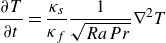
 \begin{align}&\qquad \frac {\partial T}{\partial t} + \left ( \boldsymbol{u} \boldsymbol{\cdot} \boldsymbol{\nabla} \right ) T = \frac {1}{\sqrt {Ra {Pr}}} \nabla ^{2} T. \end{align}
In contrast, the solid subdomains require us to solve a pure diffusion equation
 \begin{align} \frac {\partial T}{\partial t} &= \frac {\kappa _s}{\kappa _f} \frac {1}{\sqrt {Ra {Pr}}} \nabla ^{2} T \end{align}
only (Foroozani et al. Reference Foroozani, Krasnov and Schumacher2021; Vieweg et al. Reference Vieweg, Käufer, Cierpka and Schumacher2025). Here,
 $\boldsymbol{u}$
,
$\boldsymbol{u}$
,
 $T$
and
$T$
and
 $p$
represent the (non-dimensional) velocity, temperature and pressure fields, whereas
$p$
represent the (non-dimensional) velocity, temperature and pressure fields, whereas
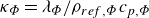 $\kappa _{\Phi } = \lambda _{\Phi } / \rho _{{ref},\Phi } c_{p,\Phi }$
is the thermal diffusivity. Its ratio between the solid and fluid domains
$\kappa _{\Phi } = \lambda _{\Phi } / \rho _{{ref},\Phi } c_{p,\Phi }$
is the thermal diffusivity. Its ratio between the solid and fluid domains
 $\kappa _s \! / \! \kappa _f$
constitutes an important control parameter over the course of this work, with the subscripts
$\kappa _s \! / \! \kappa _f$
constitutes an important control parameter over the course of this work, with the subscripts
 $\Phi =\{f,s\}$
denoting the fluid and solid, respectively. Here
$\Phi =\{f,s\}$
denoting the fluid and solid, respectively. Here
 $\lambda _{\Phi }$
represents the thermal conductivity,
$\lambda _{\Phi }$
represents the thermal conductivity,
 $\rho _{{ref},\Phi}$
the mass density and
$\rho _{{ref},\Phi}$
the mass density and
 $c_{p,\Phi }$
the specific heat capacity at constant pressure. Furthermore, the Rayleigh and Prandtl number are defined via
$c_{p,\Phi }$
the specific heat capacity at constant pressure. Furthermore, the Rayleigh and Prandtl number are defined via
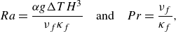 \begin{equation} Ra = \frac {\alpha g \Delta T H^{3}}{\nu _f \kappa _f} \quad \textrm {and} \quad {Pr} = \frac {\nu _f}{\kappa _f}, \end{equation}
where
 $\nu _f$
is the kinematic viscosity of the fluid . Note that (2.4) holds for both the top and bottom plate – as they will offer identical thermal diffusivities – and, thus, differs from our recent work (Vieweg et al. Reference Vieweg, Käufer, Cierpka and Schumacher2025).
$\nu _f$
is the kinematic viscosity of the fluid . Note that (2.4) holds for both the top and bottom plate – as they will offer identical thermal diffusivities – and, thus, differs from our recent work (Vieweg et al. Reference Vieweg, Käufer, Cierpka and Schumacher2025).
2.2. Numerical domain, boundary and initial conditions
These governing equations are complemented by a numerical domain and its respective boundary conditions. We define the horizontal extent
 $L$
of our numerical domain by the (horizontal) aspect ratio
$L$
of our numerical domain by the (horizontal) aspect ratio
 ${\Gamma }:=L/H$
, whereas the vertical aspect ratio
${\Gamma }:=L/H$
, whereas the vertical aspect ratio
 ${\Gamma _s}:=H_s/H$
describes the thickness of each of the surrounding solid plates. Note that both of these aspect ratios are based on the height
${\Gamma _s}:=H_s/H$
describes the thickness of each of the surrounding solid plates. Note that both of these aspect ratios are based on the height
 $H$
of the fluid domain, whereas any subdomain offers the square horizontal cross-section
$H$
of the fluid domain, whereas any subdomain offers the square horizontal cross-section
 $A={\Gamma } \times {\Gamma }$
. Regarding figure 1, the solid bottom and top domains are thus situated at
$A={\Gamma } \times {\Gamma }$
. Regarding figure 1, the solid bottom and top domains are thus situated at
 $z \in [-{\Gamma _s},0]$
and
$z \in [-{\Gamma _s},0]$
and
 $z \in [1,1+{\Gamma _s}]$
, respectively, with the fluid in between at
$z \in [1,1+{\Gamma _s}]$
, respectively, with the fluid in between at
 $z \in [0,1]$
.
$z \in [0,1]$
.
We consider a horizontally periodic domain where any quantity
 $\boldsymbol{\Phi }$
repeats according to
$\boldsymbol{\Phi }$
repeats according to
 \begin{equation} \boldsymbol{\Phi } \left ( \boldsymbol{x} \right ) = \boldsymbol{\Phi } \left ( \boldsymbol{x} + i_x L_x \boldsymbol{e}_{x} + i_y L_y \boldsymbol{e}_{y} \right ), \quad i_{x,y} \in \mathbb{N} \end{equation}
and offers no-slip boundary conditions
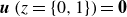 \begin{equation} \boldsymbol{u} \left (z=\{0,1\} \right ) = {\boldsymbol{0}} \end{equation}
at both solid–fluid interfaces. Thermal boundary conditions are applied in the form of constant temperatures at the very top and bottom of the plates (i.e.
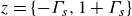 $z=\{-{\Gamma _s}, 1+{\Gamma _s}\}$
) which will further be referred to as
$z=\{-{\Gamma _s}, 1+{\Gamma _s}\}$
) which will further be referred to as
 \begin{align} T \left ( z = - {\Gamma _s} \right )&= {T_h} \quad \textrm {and} \end{align}
 \begin{align} T \left ( z = 1 + {\Gamma _s} \right )&= T_c. \end{align}
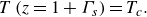
By nature of the CHT set-up, temperature fields and diffusive heat fluxes are coupled at the solid–fluid interfaces (i.e.
 $z=\left \{ 0,1 \right \}$
) according to
$z=\left \{ 0,1 \right \}$
) according to
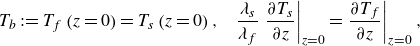 \begin{align} T_b := T_f \left ( z=0 \right ) = T_{s} \left ( z=0 \right ), & \quad \frac {\lambda _s}{\lambda _f} \left . \frac {\partial T_{s}}{\partial z}\right \rvert _{z=0} = \left . \frac {\partial T_{f}} {\partial z}\right \rvert _{z=0}, \end{align}
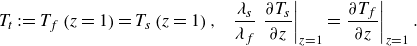 \begin{align} T_t := T_f \left ( z=1 \right ) = T_{s} \left ( z=1 \right ), & \quad \frac {\lambda _s}{\lambda _f} \left . \frac {\partial T_{s}}{\partial z}\right \rvert _{z=1} = \left . \frac {\partial T_{f}} {\partial z}\right \rvert _{z=1}. \end{align}
Note that while the energy equation (2.4) contains
 $\kappa _s \! / \! \kappa _f$
due to the non-dimensionalisation, the boundary conditions (2.10) and (2.11) include the ratio
$\kappa _s \! / \! \kappa _f$
due to the non-dimensionalisation, the boundary conditions (2.10) and (2.11) include the ratio
 $\lambda _s \! / \! \lambda _f$
to match the diffusive heat fluxes at the interfaces. In order to avoid another control parameter, we assume in our simulations
$\lambda _s \! / \! \lambda _f$
to match the diffusive heat fluxes at the interfaces. In order to avoid another control parameter, we assume in our simulations
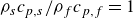 $\rho _s c_{p,s} / \rho _f c_{p,f} = 1$
such that
$\rho _s c_{p,s} / \rho _f c_{p,f} = 1$
such that
 $\lambda _s \! / \! \lambda _f \equiv \kappa _s \! / \! \kappa _f$
follows. We will thus use
$\lambda _s \! / \! \lambda _f \equiv \kappa _s \! / \! \kappa _f$
follows. We will thus use
 $\kappa _s \! / \! \kappa _f$
as the control parameter for the discussions in the main text, except for the linear stability analysis. We additionally stress that as we fix the externally applied temperatures
$\kappa _s \! / \! \kappa _f$
as the control parameter for the discussions in the main text, except for the linear stability analysis. We additionally stress that as we fix the externally applied temperatures
 $T_h$
and
$T_h$
and
 $T_c$
, see again (2.8) and (2.9), the resulting temperature fields at the solid–fluid interfaces
$T_c$
, see again (2.8) and (2.9), the resulting temperature fields at the solid–fluid interfaces
 $T_b$
and
$T_b$
and
 $T_t$
vary in both space and time by virtue of the systems dynamics.
$T_t$
vary in both space and time by virtue of the systems dynamics.
The ratio
 $\kappa _s \! / \! \kappa _f$
strongly impacts the way in which the fluid interacts with the solid and vice versa. For
$\kappa _s \! / \! \kappa _f$
strongly impacts the way in which the fluid interacts with the solid and vice versa. For
 $\kappa _s \! / \! \kappa _f \rightarrow \infty$
, the Dirichlet case is resembled where the temperatures at the solid–fluid interfaces become constant (since the solid is a much better thermal conductor). In contrast, for
$\kappa _s \! / \! \kappa _f \rightarrow \infty$
, the Dirichlet case is resembled where the temperatures at the solid–fluid interfaces become constant (since the solid is a much better thermal conductor). In contrast, for
 $\kappa _s \! / \! \kappa _f \rightarrow 0$
the Neumann case is mimicked where the vertical temperature gradient becomes constant at these interfaces (since thermal resistance through the fluid is smaller compared with the solid). A more elaborate explanation is provided in Appendix B. In this study, bridging the gap between Dirichlet and Neumann conditions, we are interested in a broad range of
$\kappa _s \! / \! \kappa _f \rightarrow 0$
the Neumann case is mimicked where the vertical temperature gradient becomes constant at these interfaces (since thermal resistance through the fluid is smaller compared with the solid). A more elaborate explanation is provided in Appendix B. In this study, bridging the gap between Dirichlet and Neumann conditions, we are interested in a broad range of
 $\kappa _s \! / \! \kappa _f$
centred around unity. Table 1 includes this ratio for a variety of natural configurations and shows that natural flows tend to offer
$\kappa _s \! / \! \kappa _f$
centred around unity. Table 1 includes this ratio for a variety of natural configurations and shows that natural flows tend to offer
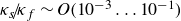 $\kappa _s \! / \! \kappa _f \sim \textit {O} (10^{-3}\ldots 10^{-1} )$
.
$\kappa _s \! / \! \kappa _f \sim \textit {O} (10^{-3}\ldots 10^{-1} )$
.
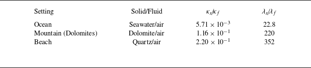
Ratios of thermophysical properties in natural configurations. Values of both the thermal diffusivity as well as thermal conductivity are taken at
 $10\,^\circ \mathrm{C}$
for seawater (salinity of 35 p.p.t.), air and quartz from Ochsner (Reference Ochsner2019), Ibrahim & Badawy (2017), and for dolomite from Stout & Robie (Reference Stout and Robie1963) and Horai (Reference Horai1971).
$10\,^\circ \mathrm{C}$
for seawater (salinity of 35 p.p.t.), air and quartz from Ochsner (Reference Ochsner2019), Ibrahim & Badawy (2017), and for dolomite from Stout & Robie (Reference Stout and Robie1963) and Horai (Reference Horai1971).
Concerning our initial condition, we follow the procedure described and introduced by Vieweg et al. (Reference Vieweg, Käufer, Cierpka and Schumacher2025). In a nutshell, we initialise each simulation with a fluid at rest, i.e.
 $\boldsymbol{u} ( \boldsymbol{x}, t=0 ) = 0$
, and linear temperature profiles which respect the internal boundary conditions between the different subdomains as outlined in (2.10) and (2.11). By adding some tiny random thermal noise
$\boldsymbol{u} ( \boldsymbol{x}, t=0 ) = 0$
, and linear temperature profiles which respect the internal boundary conditions between the different subdomains as outlined in (2.10) and (2.11). By adding some tiny random thermal noise
 $0 \leq \varUpsilon \leq 10^{-3}$
, we accelerate the transition to the statistically stationary state under the assumption of an initial Nusselt number
$0 \leq \varUpsilon \leq 10^{-3}$
, we accelerate the transition to the statistically stationary state under the assumption of an initial Nusselt number
 ${Nu} (t=0 ) \gt 1$
based on preliminary simulation runs.
${Nu} (t=0 ) \gt 1$
based on preliminary simulation runs.
The required, externally applied temperatures
 $T_h$
and
$T_h$
and
 $T_c$
(see (2.8) and (2.9)) are determined as follows. First, we define the global Nusselt number
$T_c$
(see (2.8) and (2.9)) are determined as follows. First, we define the global Nusselt number
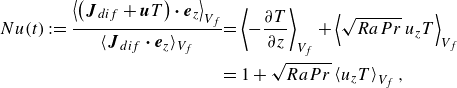 \begin{align} \nonumber {{Nu} (t) := \frac {\left \langle \left (\boldsymbol{J}_{dif} + \boldsymbol{u} T \right ) \boldsymbol{\cdot} \boldsymbol{e}_{z} \right \rangle _{V_f}}{\langle \boldsymbol{J}_{dif} \boldsymbol{\cdot} \boldsymbol{e}_{z} \rangle _{V_f}} } & { = \left \langle - \frac {\partial T }{\partial z} \right \rangle _{V_f}+ \left \langle \sqrt {Ra {Pr}} \, u_{z} T \right \rangle _{V_f} } \\ &{ = 1 + \sqrt {Ra {Pr}} \left \langle u_{z} T \right \rangle _{V_f} ,} \end{align}
as a measure of the induced amplification of the global heat transfer due to convective fluid motion. Note that the latter is associated with
 $\boldsymbol{u} T$
and in contrast to the diffusive heat current
$\boldsymbol{u} T$
and in contrast to the diffusive heat current
 $\boldsymbol{J}_{dif}$
while
$\boldsymbol{J}_{dif}$
while
 $V_f = A \times H$
represents the fluid volume (Otero et al. Reference Otero, Wittenberg, Worthing and Doering2002; Vieweg Reference Vieweg2023). Second, given the linear conduction profiles outlined in (Vieweg et al. Reference Vieweg, Käufer, Cierpka and Schumacher2025) and an assumed amplification of heat transfer as measured by
$V_f = A \times H$
represents the fluid volume (Otero et al. Reference Otero, Wittenberg, Worthing and Doering2002; Vieweg Reference Vieweg2023). Second, given the linear conduction profiles outlined in (Vieweg et al. Reference Vieweg, Käufer, Cierpka and Schumacher2025) and an assumed amplification of heat transfer as measured by
 $Nu$
, it is possible to estimate these applied temperatures – that are required to achieve
$Nu$
, it is possible to estimate these applied temperatures – that are required to achieve
 $\Delta T_N \, \approx \, 1$
– according to
$\Delta T_N \, \approx \, 1$
– according to
 \begin{equation} {{T_h} = 1 + \frac {\lambda _f}{\lambda _s} {\Gamma _s} {Nu} \quad \textrm {and} \quad T_c = - \frac {\lambda _f}{\lambda _s} {\Gamma _s} {Nu}.} \end{equation}
Note that, as the final
 $Nu$
is not known a priori, either preliminary two- and three-dimensional simulation runs or our introduced
$Nu$
is not known a priori, either preliminary two- and three-dimensional simulation runs or our introduced
 $\tanh$
-relationship (which will be discussed in § 4) have been used to find appropriate values for
$\tanh$
-relationship (which will be discussed in § 4) have been used to find appropriate values for
 $T_h$
and
$T_h$
and
 $T_c$
.
$T_c$
.
3. Linear stability analysis of the coupled system
Flow structures at the onset of convection, as derivable analytically via a linear stability analysis, are a characteristic of the dynamical system and, thus, helpful for understanding even turbulent flow structures (Pandey et al. Reference Pandey, Scheel and Schumacher2018; Vieweg et al. Reference Vieweg, Scheel and Schumacher2021). Although such a linear stability analysis yields a relation
 $Ra (k)$
, it is the global minimum of this function that determines the critical Rayleigh number
$Ra (k)$
, it is the global minimum of this function that determines the critical Rayleigh number
 $Ra_{c}$
and critical wavenumber
$Ra_{c}$
and critical wavenumber
 $k_{c}$
. If
$k_{c}$
. If
 $Ra \gtrsim Ra_{c}$
, linear perturbations grow exponentially over time and lead to the associated size or wavelength of the emerging flow structures of
$Ra \gtrsim Ra_{c}$
, linear perturbations grow exponentially over time and lead to the associated size or wavelength of the emerging flow structures of
 $\lambda _{c} = 2 \pi / k_{c}$
.
$\lambda _{c} = 2 \pi / k_{c}$
.
While, given our no-slip boundary conditions, (
 $Ra_{c}$
,
$Ra_{c}$
,
 $k_{c}$
) are well known for the Dirichlet (
$k_{c}$
) are well known for the Dirichlet (
 $Ra_{c}=1707.8, k_{c}=3.13$
) (Pellew & Southwell Reference Pellew and Southwell1940) and Neumann (
$Ra_{c}=1707.8, k_{c}=3.13$
) (Pellew & Southwell Reference Pellew and Southwell1940) and Neumann (
 $Ra_{c}=6!=720, k_{c}=0$
) (Hurle et al. Reference Hurle, Jakeman and Pike1967) cases, these values change for vertically infinitely extended (i.e.
$Ra_{c}=6!=720, k_{c}=0$
) (Hurle et al. Reference Hurle, Jakeman and Pike1967) cases, these values change for vertically infinitely extended (i.e.
 ${\Gamma _s} \rightarrow \infty$
) CHT set-ups with finite ratios of thermal conductivities
${\Gamma _s} \rightarrow \infty$
) CHT set-ups with finite ratios of thermal conductivities
 $\lambda _s \! / \! \lambda _f \in ( 0, \infty )$
(Hurle et al. Reference Hurle, Jakeman and Pike1967). One can expect that a finite plate thickness
$\lambda _s \! / \! \lambda _f \in ( 0, \infty )$
(Hurle et al. Reference Hurle, Jakeman and Pike1967). One can expect that a finite plate thickness
 $\Gamma _s$
adds an additional layer of complexity.
$\Gamma _s$
adds an additional layer of complexity.
This study extends the work of Hurle et al. (Reference Hurle, Jakeman and Pike1967) by (i) investigating a broader range of
 $\lambda _s \! / \! \lambda _f$
, (ii) considering even finite plate thicknesses
$\lambda _s \! / \! \lambda _f$
, (ii) considering even finite plate thicknesses
 $\Gamma _s$
(in § 6) and (iii) deriving easy-to-handle relationships between
$\Gamma _s$
(in § 6) and (iii) deriving easy-to-handle relationships between
 $Ra_{c}$
,
$Ra_{c}$
,
 $k_{c}$
and
$k_{c}$
and
 $\lambda _s \! / \! \lambda _f$
.
$\lambda _s \! / \! \lambda _f$
.
In order to determine the neutral stability curve and subsequently derive
 $Ra_{c}$
as well as
$Ra_{c}$
as well as
 $k_{c}$
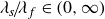
, a system of four equations needs to be solved where the determinant of the coefficient matrix
$k_{c}$
, a system of four equations needs to be solved where the determinant of the coefficient matrix
 $\boldsymbol{M_E}$
is set to zero to obtain a non-trivial solution,
$\boldsymbol{M_E}$
is set to zero to obtain a non-trivial solution,
 \begin{align} &\det {\boldsymbol{M_E}} \stackrel {!}{=} 0 = \left \rvert \begin{matrix} 0 & 1 & 1 & 1 \\ 0 & q_1t_1 & q_2t_2 & q_3t_3 \\ - \frac {\lambda _f}{\lambda _s} \tanh {\left (k{\Gamma _s} \right )} & \gamma & -\frac {\gamma }{2} \left ( 1-\mathrm{i} \sqrt {3} \right ) & -\frac {\gamma }{2} \left ( 1-\mathrm{i} \sqrt {3} \right ) \\ k & \gamma q_1t_1 & -\frac {\gamma }{2} \left ( 1-\mathrm{i} \sqrt {3} \right ) q_2t_2 & -\frac {\gamma }{2} \left ( 1-\mathrm{i} \sqrt {3} \right ) q_3t_3 \end{matrix} \right \rvert . \end{align}
In the following, we only regard the case of even modes as it provides the lower values for
 $Ra_{c}$
. A detailed derivation – explaining all involved variables – is provided in Appendix A.
$Ra_{c}$
. A detailed derivation – explaining all involved variables – is provided in Appendix A.
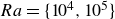
Linear stability of CHT-driven Rayleigh–Bénard convection. The combination of thermophysical properties controls both the general stability (
 $Ra_{c}$
) as well as the size of the critical flow structures (
$Ra_{c}$
) as well as the size of the critical flow structures (
 $k_{c}$
). (a) Different neutral stability curves indicate (c) a gradual and monotonic transition of both
$k_{c}$
). (a) Different neutral stability curves indicate (c) a gradual and monotonic transition of both
 $Ra_{c}$
and
$Ra_{c}$
and
 $k_{c}$
(see also panels (d) and (b), respectively). The true solutions from panels (b–d) can be approximated well by tanh- or polynomial-based regressions using parameters described by table 2. Note the different convergence behaviour of
$k_{c}$
(see also panels (d) and (b), respectively). The true solutions from panels (b–d) can be approximated well by tanh- or polynomial-based regressions using parameters described by table 2. Note the different convergence behaviour of
 $k_{c}$
for
$k_{c}$
for
 $\lambda _s \! / \! \lambda _f \rightarrow \infty$
(
$\lambda _s \! / \! \lambda _f \rightarrow \infty$
(
 $k_{c} = \mathrm{const.}$
) and
$k_{c} = \mathrm{const.}$
) and
 $\lambda _s \! / \! \lambda _f \rightarrow 0$
(
$\lambda _s \! / \! \lambda _f \rightarrow 0$
(
 $k_{c} \sim ( \lambda _s \! / \! \lambda _f )^{1/3}$
) as highlighted by the inset in panel (b), the latter of which plots the data double-logarithmically instead.
$k_{c} \sim ( \lambda _s \! / \! \lambda _f )^{1/3}$
) as highlighted by the inset in panel (b), the latter of which plots the data double-logarithmically instead.

Figure 2(a) contrasts different resulting neutral stability curves for different
 $\lambda _s \! / \! \lambda _f$
given
$\lambda _s \! / \! \lambda _f$
given
 ${\Gamma _s} \rightarrow \infty$
. Remember that the extreme cases
${\Gamma _s} \rightarrow \infty$
. Remember that the extreme cases
 $\lambda _s \! / \! \lambda _f=\left \{10^{-6}, 10^{6} \right \}$
mimic the Neumann and Dirichlet cases, respectively, and with which they correspond (Pellew & Southwell Reference Pellew and Southwell1940; Chandrasekhar Reference Chandrasekhar1981; Takehiro et al. Reference Takehiro, Ishiwatari, Nakajima and Hayashi2002). Interestingly, after having solved (3.1) for a large number of
$\lambda _s \! / \! \lambda _f=\left \{10^{-6}, 10^{6} \right \}$
mimic the Neumann and Dirichlet cases, respectively, and with which they correspond (Pellew & Southwell Reference Pellew and Southwell1940; Chandrasekhar Reference Chandrasekhar1981; Takehiro et al. Reference Takehiro, Ishiwatari, Nakajima and Hayashi2002). Interestingly, after having solved (3.1) for a large number of
 $\lambda _s \! / \! \lambda _f$
, we find a gradual and monotonic transition for both
$\lambda _s \! / \! \lambda _f$
, we find a gradual and monotonic transition for both
 $Ra_{c}$
and
$Ra_{c}$
and
 $k_{c}$
in between these extreme conditions as visualised in figure 2(b–d). Our analysis shows that the onset of convection is generally delayed (i.e. larger
$k_{c}$
in between these extreme conditions as visualised in figure 2(b–d). Our analysis shows that the onset of convection is generally delayed (i.e. larger
 $Ra_{c}$
) with smaller emerging flow structures (i.e. larger
$Ra_{c}$
) with smaller emerging flow structures (i.e. larger
 $k_{c}$
) for relatively better solid thermal conductors (i.e. increasing
$k_{c}$
) for relatively better solid thermal conductors (i.e. increasing
 $\lambda _s \! / \! \lambda _f$
). As highlighted by the inset in figure 2(b),
$\lambda _s \! / \! \lambda _f$
). As highlighted by the inset in figure 2(b),
 $k_{c} ( \lambda _s \! / \! \lambda _f )$
exhibits different asymptotic convergence behaviours for the extremes of
$k_{c} ( \lambda _s \! / \! \lambda _f )$
exhibits different asymptotic convergence behaviours for the extremes of
 $\lambda _s \! / \! \lambda _f$
: While
$\lambda _s \! / \! \lambda _f$
: While
 $k_{c} \sim \lambda _s \! / \! \lambda _f^{1/3}$
for
$k_{c} \sim \lambda _s \! / \! \lambda _f^{1/3}$
for
 $\lambda _s \! / \! \lambda _f \rightarrow 0$
,
$\lambda _s \! / \! \lambda _f \rightarrow 0$
,
 $k_{c} \simeq 3.13 = \textrm {const.}$
for
$k_{c} \simeq 3.13 = \textrm {const.}$
for
 $\lambda _s \! / \! \lambda _f \rightarrow \infty$
. Interestingly, the inflection point is around
$\lambda _s \! / \! \lambda _f \rightarrow \infty$
. Interestingly, the inflection point is around
 $\lambda _s \! / \! \lambda _f \approx 10^{-3/4}$
(rather than
$\lambda _s \! / \! \lambda _f \approx 10^{-3/4}$
(rather than
 $10^{0}$
) and thus introduces an asymmetry with respect to
$10^{0}$
) and thus introduces an asymmetry with respect to
 $\lambda _s \! / \! \lambda _f$
.
$\lambda _s \! / \! \lambda _f$
.
These (true) solutions are the result of solving (3.1). In order to provide handier solutions that are more accessible, we apply tanh- or polynomial-based regressions to the original data from figure 2(b–d) and include them therein. Given the parameters shown in table 2, such simple regression fits approximate the true solutions (very) well.
Albeit this linear stability analysis is based on
 ${\Gamma _s} \rightarrow \infty$
, we find that its solutions practically coincide with our numerically employed finite case
${\Gamma _s} \rightarrow \infty$
, we find that its solutions practically coincide with our numerically employed finite case
 ${\Gamma _s} = 15$
as shown in § 6.
${\Gamma _s} = 15$
as shown in § 6.
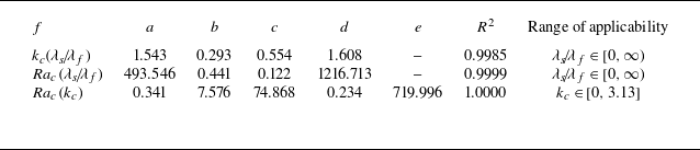
Regression parameters for
 $k_{c}$
and
$k_{c}$
and
 $Ra_{c}$
. A
$Ra_{c}$
. A
 $\tanh$
-fit of the form
$\tanh$
-fit of the form
 $f (\lambda _s \! / \! \lambda _f, Ra ) = a \tanh { [ b {\rm In} { ( \lambda _s \! / \! \lambda _f ) } + c ] } + d$
is applied to the values in figure 2 (a,b). For
$f (\lambda _s \! / \! \lambda _f, Ra ) = a \tanh { [ b {\rm In} { ( \lambda _s \! / \! \lambda _f ) } + c ] } + d$
is applied to the values in figure 2 (a,b). For
 $Ra_{c} ( k_{c} )$
in figure 2(c), a fourth-order polynomial fit of the form
$Ra_{c} ( k_{c} )$
in figure 2(c), a fourth-order polynomial fit of the form
 $f (k_{c} ) = a k_{c}^4 + b k_{c}^3 + c k_{c}^2 + d k_{c} + e$
is applied. Here
$f (k_{c} ) = a k_{c}^4 + b k_{c}^3 + c k_{c}^2 + d k_{c} + e$
is applied. Here
 $R^2$
is the coefficient of determination (Wright Reference Wright1921) and underlines the quality of these fits.
$R^2$
is the coefficient of determination (Wright Reference Wright1921) and underlines the quality of these fits.
4. Nonlinear pattern formation
4.1. Conducted simulations and pattern formation process
In order to systematically investigate the impact of natural thermal boundary conditions on convection flows beyond their onset, we conduct two main series of simulations at two
 $Ra$
varying
$Ra$
varying
 $\kappa _s \! / \! \kappa _f$
across a broad range. For all these simulations, the Prandtl number
$\kappa _s \! / \! \kappa _f$
across a broad range. For all these simulations, the Prandtl number
 ${Pr}=1$
, horizontal aspect ratio
${Pr}=1$
, horizontal aspect ratio
 ${\Gamma }=30$
and vertical aspect ratio
${\Gamma }=30$
and vertical aspect ratio
 ${\Gamma _s}=15$
. Our choice of such a horizontally extended domain makes the heat and momentum transfer, as quantified by
${\Gamma _s}=15$
. Our choice of such a horizontally extended domain makes the heat and momentum transfer, as quantified by
 $Nu$
and
$Nu$
and
 $\rm Re$
, independent of
$\rm Re$
, independent of
 $\Gamma$
(Stevens et al. Reference Stevens, Blass, Zhu, Verzicco and Lohse2018) and delays limiting the pattern formation process by the horizontal extent of the domain (Stevens et al. Reference Stevens, Blass, Zhu, Verzicco and Lohse2018; Krug et al. Reference Krug, Lohse and Stevens2020; Vieweg Reference Vieweg2023) as further discussed in § 4.3. We report a third series of simulations at different
$\Gamma$
(Stevens et al. Reference Stevens, Blass, Zhu, Verzicco and Lohse2018) and delays limiting the pattern formation process by the horizontal extent of the domain (Stevens et al. Reference Stevens, Blass, Zhu, Verzicco and Lohse2018; Krug et al. Reference Krug, Lohse and Stevens2020; Vieweg Reference Vieweg2023) as further discussed in § 4.3. We report a third series of simulations at different
 $\Gamma _s$
given
$\Gamma _s$
given
 $\kappa _s \! / \! \kappa _f=10^0$
in § 6 whereas we contrast extreme cases of
$\kappa _s \! / \! \kappa _f=10^0$
in § 6 whereas we contrast extreme cases of
 $\kappa _s \! / \! \kappa _f$
with their plateless classical representatives in Appendix B.
$\kappa _s \! / \! \kappa _f$
with their plateless classical representatives in Appendix B.
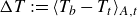
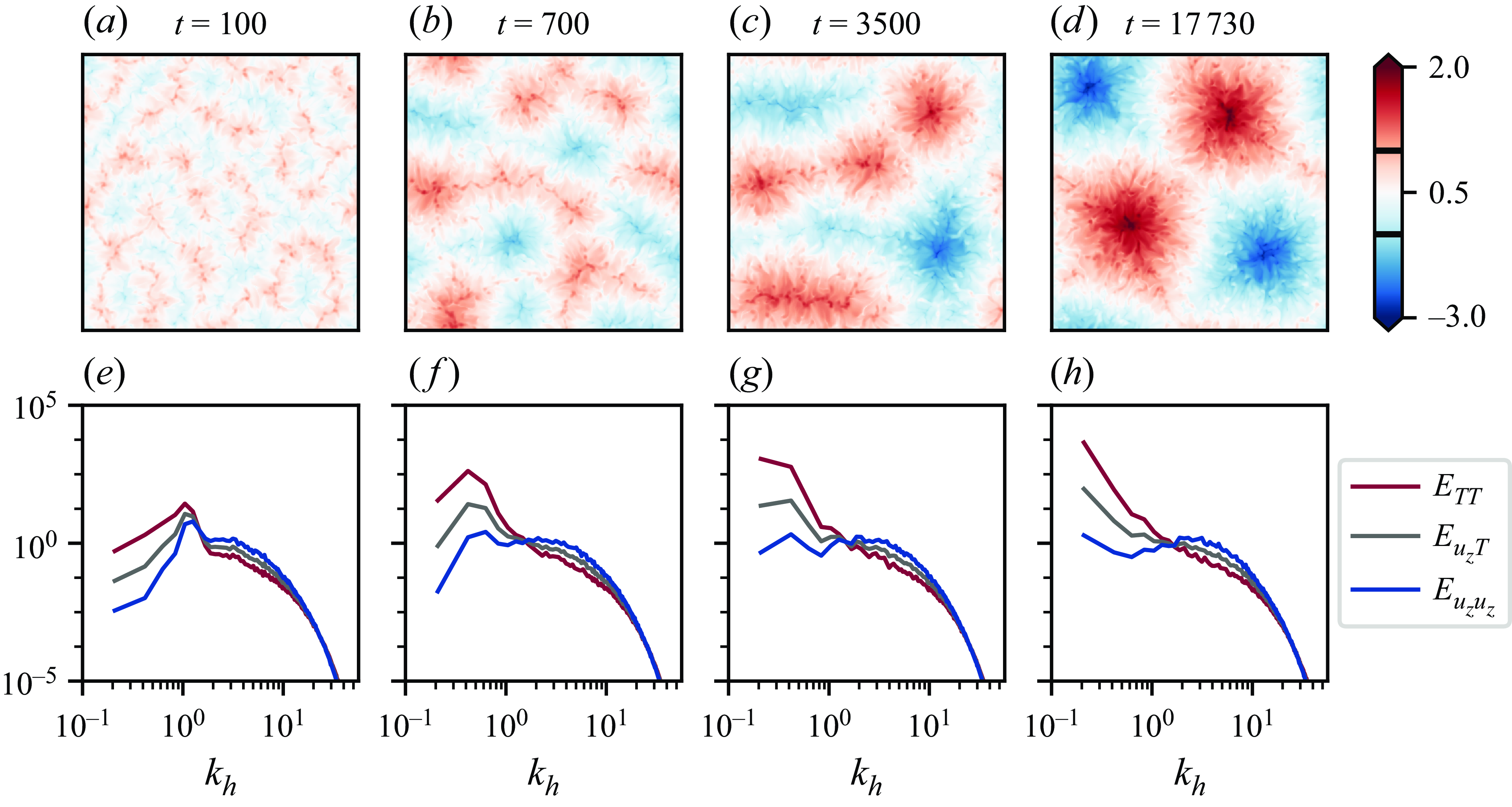
Gradual pattern formation. (a) At early times, large-scale granulated flow structures emerge that (b,c) gradually merge and form even larger supergranules before (d) a statistically stationary state is reached. Here we visualise the thermal footprint
 $T ( x, y, z = 0.5, t )$
of these flow structures. (e–h) The corresponding azimuthally averaged Fourier energy spectra (of various fields) highlight a gradual shift of spectral energy towards larger horizontal scales. This shift is governed by
$T ( x, y, z = 0.5, t )$
of these flow structures. (e–h) The corresponding azimuthally averaged Fourier energy spectra (of various fields) highlight a gradual shift of spectral energy towards larger horizontal scales. This shift is governed by
 $\kappa _s \! / \! \kappa _f$
, as
$\kappa _s \! / \! \kappa _f$
, as
 $\kappa _s \! / \! \kappa _f \rightarrow 0$
, more energy accumulates at even smaller
$\kappa _s \! / \! \kappa _f \rightarrow 0$
, more energy accumulates at even smaller
 $k_h$
. In contrast to the idealised Neumann case – compare with (Vieweg et al. Reference Vieweg, Scheel and Schumacher2021) – the growth of the supergranules stops in this CHT set-up of
$k_h$
. In contrast to the idealised Neumann case – compare with (Vieweg et al. Reference Vieweg, Scheel and Schumacher2021) – the growth of the supergranules stops in this CHT set-up of
 $Ra=10^5$
and
$Ra=10^5$
and
 $\kappa _s \! / \! \kappa _f=10^0$
(Case
$\kappa _s \! / \! \kappa _f=10^0$
(Case
 $\mathrm{C5c}$
) before reaching domain size.
$\mathrm{C5c}$
) before reaching domain size.
Convective pattern formation is known to be a gradual process which reaches statistically stationary flow structures only after a long time, potentially even
 $\textit {O} ( 10^4 \tau _f )$
or longer (Vieweg et al. Reference Vieweg, Scheel and Schumacher2021, Reference Vieweg, Scheel, Stepanov and Schumacher2022, Reference Vieweg, Klünker, Schumacher and Padberg-Gehle2024; Vieweg Reference Vieweg2023, Reference Vieweg2024a
). Figure 3 illustrates this process for one of our present CHT cases: at the beginning, granulated flow structures manifest that merge over time towards larger structures. While figure 3(a–c) depict the transient regime, figure 3(d) illustrates the flow structures by means of their thermal footprint at their statistically stationary state. Reaching this late regime has successfully been probed using different measures such as the integral length scale (Parodi et al. Reference Parodi, von Hardenberg, Passoni, Provenzale and Spiegel2004; Vieweg et al. Reference Vieweg, Scheel, Stepanov and Schumacher2022)
$\textit {O} ( 10^4 \tau _f )$
or longer (Vieweg et al. Reference Vieweg, Scheel and Schumacher2021, Reference Vieweg, Scheel, Stepanov and Schumacher2022, Reference Vieweg, Klünker, Schumacher and Padberg-Gehle2024; Vieweg Reference Vieweg2023, Reference Vieweg2024a
). Figure 3 illustrates this process for one of our present CHT cases: at the beginning, granulated flow structures manifest that merge over time towards larger structures. While figure 3(a–c) depict the transient regime, figure 3(d) illustrates the flow structures by means of their thermal footprint at their statistically stationary state. Reaching this late regime has successfully been probed using different measures such as the integral length scale (Parodi et al. Reference Parodi, von Hardenberg, Passoni, Provenzale and Spiegel2004; Vieweg et al. Reference Vieweg, Scheel, Stepanov and Schumacher2022)
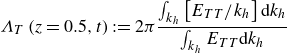 \begin{equation} \varLambda _T \left ( z = 0.5, t \right ) := 2 \pi \frac {\int _{k_{h}} \left [ E_{TT} / k_{h} \right ] {\rm d}k_{h}}{\int _{k_{h}} E_{TT} {\rm d}k_{h}} \end{equation}
with
 $E_{TT} \equiv E_{TT} ( k_{h}, z = 0.5, t )$
representing the azimuthally averaged Fourier energy spectrum of the temperature field and
$E_{TT} \equiv E_{TT} ( k_{h}, z = 0.5, t )$
representing the azimuthally averaged Fourier energy spectrum of the temperature field and
 $k_{h}$
the horizontal wavenumber, or the thermal variance (Vieweg et al. Reference Vieweg, Scheel, Stepanov and Schumacher2022)
$k_{h}$
the horizontal wavenumber, or the thermal variance (Vieweg et al. Reference Vieweg, Scheel, Stepanov and Schumacher2022)
 \begin{equation} \varTheta _{rms} \left ( t \right ) := \sqrt {\langle \varTheta ^2 \rangle _V} \quad \textrm {with} \quad \varTheta (\boldsymbol{x},t) := T(\boldsymbol{x},t) - T_{lin}(z) \end{equation}
where
 $\varTheta _{rms}$
is the temperature deviation field around the mean linear conduction profile
$\varTheta _{rms}$
is the temperature deviation field around the mean linear conduction profile
 $T_{lin} = 1-z$
across the fluid domain (Vieweg Reference Vieweg2023, Reference Vieweg2024a
). In case of Neumann-type thermal boundary conditions,
$T_{lin} = 1-z$
across the fluid domain (Vieweg Reference Vieweg2023, Reference Vieweg2024a
). In case of Neumann-type thermal boundary conditions,
 $\varLambda _T$
usually converges more quickly than
$\varLambda _T$
usually converges more quickly than
 $\varTheta _{rms}$
(Vieweg Reference Vieweg2023).
$\varTheta _{rms}$
(Vieweg Reference Vieweg2023).
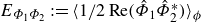
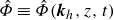
Figure 3(e–h) demonstrate how various azimuthally averaged Fourier energy spectra develop over the course of this gradual aggregation process. Here, given
 $E_{\Phi_{1} \Phi_{2}} := \langle 1/2 \, \textrm{Re} (\hat{\Phi}_{1}\hat{\Phi}_{2}^{*} ) \rangle_{\phi }$
with the Fourier coefficients
$E_{\Phi_{1} \Phi_{2}} := \langle 1/2 \, \textrm{Re} (\hat{\Phi}_{1}\hat{\Phi}_{2}^{*} ) \rangle_{\phi }$
with the Fourier coefficients
 $\hat {\Phi } \equiv \hat {\Phi } ( \boldsymbol{k}_{h}, z, t )$
and azimuthal angle
$\hat {\Phi } \equiv \hat {\Phi } ( \boldsymbol{k}_{h}, z, t )$
and azimuthal angle
 $\phi$
, we include the averaged spectra associated with the temperature field
$\phi$
, we include the averaged spectra associated with the temperature field
 $E_{TT}$
, vertical convective heat flux
$E_{TT}$
, vertical convective heat flux
 $E_{u_{z} T}$
and vertical velocity
$E_{u_{z} T}$
and vertical velocity
 $E_{u_{z} u_{z}}$
as a function of the absolute horizontal wavenumber
$E_{u_{z} u_{z}}$
as a function of the absolute horizontal wavenumber
 $k_h$
. As pattern formation progresses, spectral energy shifts towards smaller
$k_h$
. As pattern formation progresses, spectral energy shifts towards smaller
 $k_h$
– i.e. larger structures – across all of these spectra, thereby underlining the increasing dominance of large-scale flow structures. However, in comparison with the Neumann case described in Vieweg et al. (Reference Vieweg, Scheel and Schumacher2021) or Vieweg (Reference Vieweg2023), the aggregation process in the CHT set-up may cease before reaching the domain size – depending on
$k_h$
– i.e. larger structures – across all of these spectra, thereby underlining the increasing dominance of large-scale flow structures. However, in comparison with the Neumann case described in Vieweg et al. (Reference Vieweg, Scheel and Schumacher2021) or Vieweg (Reference Vieweg2023), the aggregation process in the CHT set-up may cease before reaching the domain size – depending on
 $\kappa _s \! / \! \kappa _f$
. This dependence between the final size of flow structures (as quantified by
$\kappa _s \! / \! \kappa _f$
. This dependence between the final size of flow structures (as quantified by
 $\varLambda _T$
, see again (4.1)) and
$\varLambda _T$
, see again (4.1)) and
 $\kappa _s \! / \! \kappa _f$
will be analysed in more detail in § 4.3.
$\kappa _s \! / \! \kappa _f$
will be analysed in more detail in § 4.3.
In this work, due to the inclusion of solid subdomains and thus the two solid–fluid interfaces, we complement the above measures by the dynamically manifesting temperature drop
 $\Delta T_N$
across the fluid layer. We find that this measure requires similar time scales of convergence with particularly large times observed for moderate
$\Delta T_N$
across the fluid layer. We find that this measure requires similar time scales of convergence with particularly large times observed for moderate
 $\kappa _s \! / \! \kappa _f \in [ 10^{-1}, 10^{1/2} ]$
. Note that we always require the temperature drop across the fluid layer
$\kappa _s \! / \! \kappa _f \in [ 10^{-1}, 10^{1/2} ]$
. Note that we always require the temperature drop across the fluid layer
 $\Delta T_N \simeq 1$
(so the non-dimensionalisation for (2.1)–(2.4) holds) whereas the temperature drop across each solid plate
$\Delta T_N \simeq 1$
(so the non-dimensionalisation for (2.1)–(2.4) holds) whereas the temperature drop across each solid plate
 $ ( {T_h} - T_c -1 ) / 2$
depends strongly on
$ ( {T_h} - T_c -1 ) / 2$
depends strongly on
 $\kappa _s \! / \! \kappa _f$
.
$\kappa _s \! / \! \kappa _f$
.
Starting from initial conditions as described in § 2.2, we run each numerical simulation as long as necessary to reach the late statistically stationary regime (probed by
 $\varLambda _T$
,
$\varLambda _T$
,
 $\varTheta _{rms}$
and
$\varTheta _{rms}$
and
 $\Delta T_N$
) and cover the latter for an extended period of time. Table 3 summarises the simulation parameters for all of our simulation runs.
$\Delta T_N$
) and cover the latter for an extended period of time. Table 3 summarises the simulation parameters for all of our simulation runs.
Simulation parameters. The Prandtl number
 ${Pr} \! = \! 1$
in a horizontally periodic domain of (horizontal) aspect ratio
${Pr} \! = \! 1$
in a horizontally periodic domain of (horizontal) aspect ratio
 ${\Gamma } \! = \! 30$
and no-slip conditions at the two solid–fluid interfaces. The table contains beside the identifier further the Rayleigh number
${\Gamma } \! = \! 30$
and no-slip conditions at the two solid–fluid interfaces. The table contains beside the identifier further the Rayleigh number
 $Ra$
, the thermal diffusivity ratio
$Ra$
, the thermal diffusivity ratio
 $\kappa _s \! / \! \kappa _f$
, the vertical aspect ratio (or thickness)
$\kappa _s \! / \! \kappa _f$
, the vertical aspect ratio (or thickness)
 $\Gamma _s$
of each of the two adjacent solid plates, the total number of spectral elements
$\Gamma _s$
of each of the two adjacent solid plates, the total number of spectral elements
 $N_{e} \! = \! N_{e,x} \! \times \! N_{e,y} \! \times \! ( N_{e,z,f} \! + \! 2 \! \times N_{e,z,s} \! )$
, the polynomial order
$N_{e} \! = \! N_{e,x} \! \times \! N_{e,y} \! \times \! ( N_{e,z,f} \! + \! 2 \! \times N_{e,z,s} \! )$
, the polynomial order
 $N$
of each spectral element, the total simulation runtime
$N$
of each spectral element, the total simulation runtime
 $t_r$
and the applied mean temperature drop across each solid plate
$t_r$
and the applied mean temperature drop across each solid plate
 $( {T_h} - T_c - 1 ) \! / 2$
.
$( {T_h} - T_c - 1 ) \! / 2$
.
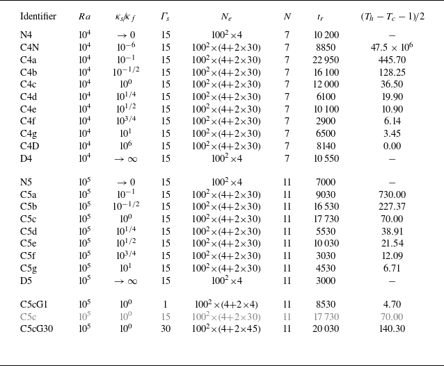
Figure 4 underlines the increased complexity of these simulations due to the added solid subdomains and their coupled interaction with the fluid layer. While we apply Dirichlet-type fixed temperatures at the very top and bottom of the domain – see figure 4(a,d) – the local heat flux at these planes may vary in space and time as visualised in figure 4(e,h). The coupled heat transfer at the two solid–fluid interfaces implies that we control neither the temperature nor the local heat flux (see figures 4(b,c) or 4(f,g), respectively) allowing for significantly weaker constraints on the dynamical fluid system. Interestingly, we find the vertical temperature gradient fields not only to be strongly negatively correlated across the fluid layer (i.e. between planes
 $z_{0} = \left \{ 0, 1 \right \}$
) but also across the entire solid–fluid–solid domain (i.e. between planes
$z_{0} = \left \{ 0, 1 \right \}$
) but also across the entire solid–fluid–solid domain (i.e. between planes
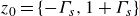 $z_0=\left \{- {\Gamma _s}, 1 + {\Gamma _s} \right \}$
) despite
$z_0=\left \{- {\Gamma _s}, 1 + {\Gamma _s} \right \}$
) despite
 ${\Gamma _s} = 15$
. The temperature fields, on the other hand, appear to be shifted from generally warmer temperatures at
${\Gamma _s} = 15$
. The temperature fields, on the other hand, appear to be shifted from generally warmer temperatures at
 $z_0=0$
to colder ones at
$z_0=0$
to colder ones at
 $z_0=1$
while still showing the footprint of the underlying flow structures. This underlines the pronounced interplay between solid thermal capacities and the fluid flow.
$z_0=1$
while still showing the footprint of the underlying flow structures. This underlines the pronounced interplay between solid thermal capacities and the fluid flow.
4.2. Convective flow patterns for different
 $\kappa _s \! / \! \kappa _f$

We start by resembling the classical, well-known Neumann- (Vieweg et al. Reference Vieweg, Scheel and Schumacher2021; Vieweg Reference Vieweg2023) and Dirichlet-type (Pandey et al. Reference Pandey, Scheel and Schumacher2018; Vieweg et al. Reference Vieweg, Scheel and Schumacher2021) thermal boundary conditions using our CHT set-up subjected to the extreme
 $\kappa _s \! / \! \kappa _f = \left \{ 10^{-6}, 10^{6} \right \}$
. Appendix B contrasts the resulting flow structures – which are commonly distinguished, respectively, as supergranules (Vieweg et al. Reference Vieweg, Scheel and Schumacher2021) and turbulent superstructures (Pandey et al. Reference Pandey, Scheel and Schumacher2018) (or spiral defect chaos for this lower
$\kappa _s \! / \! \kappa _f = \left \{ 10^{-6}, 10^{6} \right \}$
. Appendix B contrasts the resulting flow structures – which are commonly distinguished, respectively, as supergranules (Vieweg et al. Reference Vieweg, Scheel and Schumacher2021) and turbulent superstructures (Pandey et al. Reference Pandey, Scheel and Schumacher2018) (or spiral defect chaos for this lower
 $Ra$
) – and confirms a convergence of the flow for plateless and CHT configurations.
$Ra$
) – and confirms a convergence of the flow for plateless and CHT configurations.
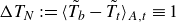
Conjugate heat transfer. In the coupled system, both the temperature (a–d) and heat flux (e–h) are coupled at the two solid–fluid interfaces (b,c,f,g) while only the temperature field is controlled at the very bottom (a) and top (d). The respective local heat flux (e,h) is still correlated. Here
 $Ra = 10^{5}$
,
$Ra = 10^{5}$
,
 ${\Gamma _s} = 15$
, and
${\Gamma _s} = 15$
, and
 $\kappa _s \! / \! \kappa _f = 10^{0}$
(i.e. case C4c). Note that when
$\kappa _s \! / \! \kappa _f = 10^{0}$
(i.e. case C4c). Note that when
 $\kappa _s \! / \! \kappa _f \rightarrow \infty$
or
$\kappa _s \! / \! \kappa _f \rightarrow \infty$
or
 $\kappa _s \! / \! \kappa _f \rightarrow 0$
, either (b,c) or (f,g) become constant, respectively.
$\kappa _s \! / \! \kappa _f \rightarrow 0$
, either (b,c) or (f,g) become constant, respectively.
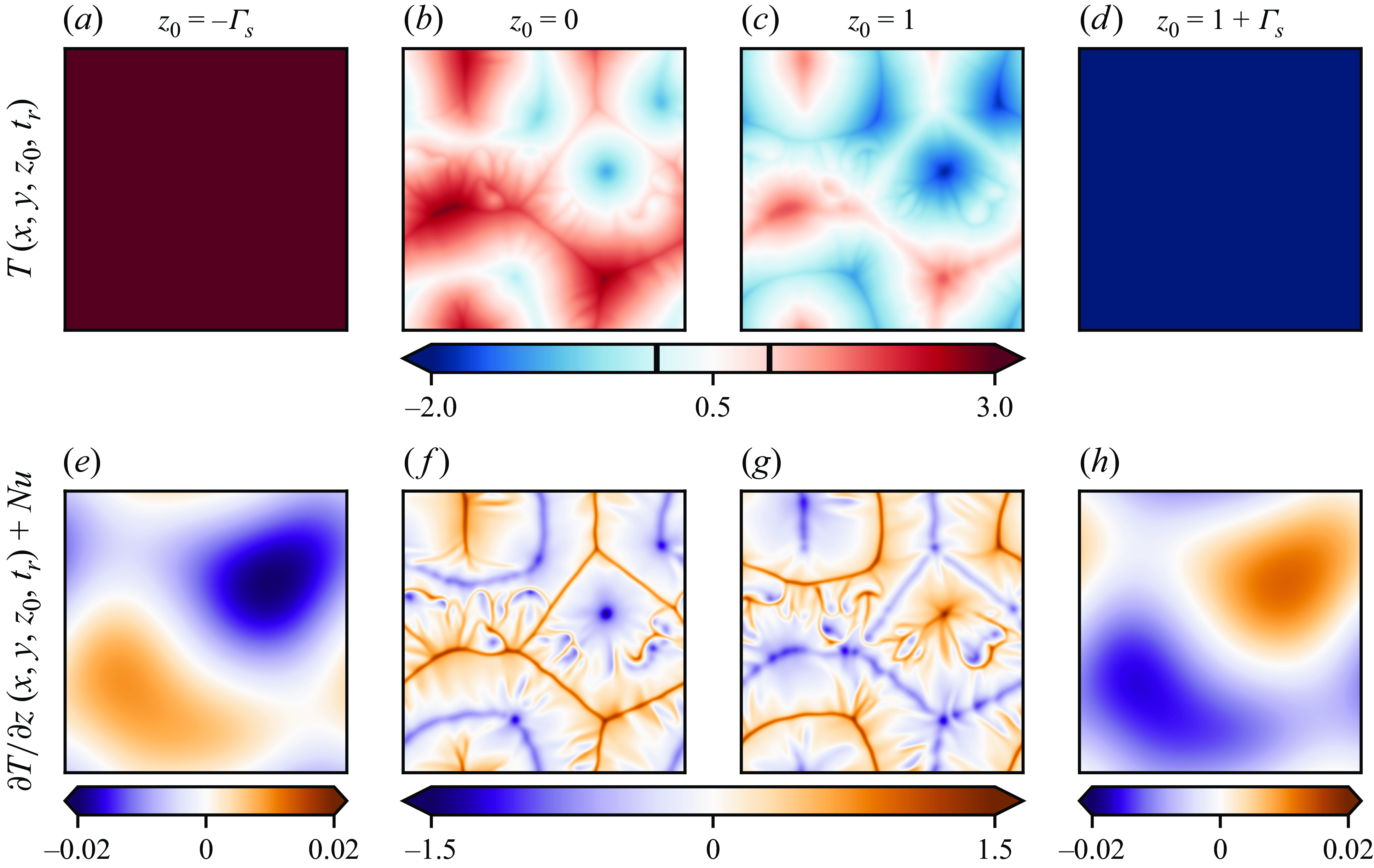
Nonlinear pattern formation. Worse solid thermal conductors (relative to the fluid) lead to the formation of larger flow structures. Here we visualise the instantaneous temperature fields
 $T ( x, y, z = 0.5, t = t_{\textrm {r}} )$
given
$T ( x, y, z = 0.5, t = t_{\textrm {r}} )$
given
 ${\Gamma _s} = 15$
. Identifiers for the runs (see the top-right of each panel) are listed in table 3.
${\Gamma _s} = 15$
. Identifiers for the runs (see the top-right of each panel) are listed in table 3.
Bridging the gap between these previously studied idealised conditions, figure 5 visualises snapshots of our simulations applying natural thermal boundary conditions covering the range
 $10^{-1} \leqslant \kappa _s \! / \! \kappa _f \leqslant 10^{1}$
. Our simulations show that smaller
$10^{-1} \leqslant \kappa _s \! / \! \kappa _f \leqslant 10^{1}$
. Our simulations show that smaller
 $\kappa _s \! / \! \kappa _f$
lead gradually to increased flow structures given a sufficiently extended domain. In our case, the growth of the flow structures is limited by the numerically finite horizontal domain size
$\kappa _s \! / \! \kappa _f$
lead gradually to increased flow structures given a sufficiently extended domain. In our case, the growth of the flow structures is limited by the numerically finite horizontal domain size
 ${\Gamma } = 30$
at
${\Gamma } = 30$
at
 $\kappa _s \! / \! \kappa _f = 10^{-1/2}$
and below. Although we study a limited range of
$\kappa _s \! / \! \kappa _f = 10^{-1/2}$
and below. Although we study a limited range of
 $\kappa _s \! / \! \kappa _f$
around unity only, it is sufficient to indicate the clear convergence towards either supergranules or turbulent superstructures. This gradual transition from one of the latter to the other suggests covering them both under the umbrella term of long-living large-scale flow structures. Our numerical results for
$\kappa _s \! / \! \kappa _f$
around unity only, it is sufficient to indicate the clear convergence towards either supergranules or turbulent superstructures. This gradual transition from one of the latter to the other suggests covering them both under the umbrella term of long-living large-scale flow structures. Our numerical results for
 $Ra \gg Ra_{c}$
are in line with the general, monotonic trend suggested by the linear stability analysis from § 3. Independently of
$Ra \gg Ra_{c}$
are in line with the general, monotonic trend suggested by the linear stability analysis from § 3. Independently of
 $\kappa _s \! / \! \kappa _f$
, we find that a larger
$\kappa _s \! / \! \kappa _f$
, we find that a larger
 $Ra$
introduces stronger turbulence on smaller scales including the granular scale (Vieweg et al. Reference Vieweg, Scheel and Schumacher2021; Vieweg Reference Vieweg2023).
$Ra$
introduces stronger turbulence on smaller scales including the granular scale (Vieweg et al. Reference Vieweg, Scheel and Schumacher2021; Vieweg Reference Vieweg2023).
4.3. Quantitative analysis of convective flow patterns
We proceed by quantifying selected aspects of our flow structures as well as their induced statistical properties. Firstly, we measure the strength of appearing thermal inhomogeneities at the two solid–fluid interfaces based on both the instantaneous maximum horizontal temperature difference
 \begin{equation} \max \left ( \varDelta _h T \right ) \left ( t \right ) := \max _{x, y} \left ( T \right ) - \min _{x, y} \left ( T \right ) \end{equation}
and the standard deviation
 $\mathrm{std} ( T )$
for
$\mathrm{std} ( T )$
for
 $T \in \{T_b, T_t \}$
. This is complemented by the induced global momentum transfer as measured by the Reynolds number (Scheel & Schumacher Reference Scheel and Schumacher2017)
$T \in \{T_b, T_t \}$
. This is complemented by the induced global momentum transfer as measured by the Reynolds number (Scheel & Schumacher Reference Scheel and Schumacher2017)
 \begin{equation} {Re} (t) := \sqrt {\frac {Ra}{{Pr}}} \, u_{rms} \quad \textrm {with} \quad u_{rms} := \sqrt { \big \langle \boldsymbol{u}^{2} \big \rangle _{V} } . \end{equation}
Thirdly, we measure the size or horizontal extent of flow structures based on the integral length scale
 $\varLambda _T$
as defined in (4.1).
$\varLambda _T$
as defined in (4.1).
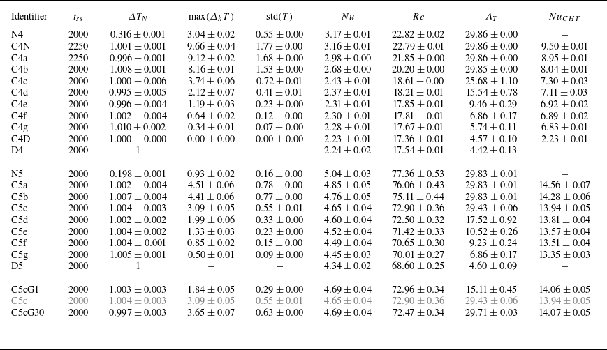
Table 4 summarises the temporal averages and associated temporal standard deviations for all our simulations. Note that this analysis covers an extended period
 $t_{ss}$
of the late statistically stationary regime of pattern formation rather than a single snapshot.
$t_{ss}$
of the late statistically stationary regime of pattern formation rather than a single snapshot.
Thermal and global characteristics of the direct numerical simulations listed in table 3. The table contains the analysis time interval in the statistically stationary regime
 $t_{ss}$
(being part of
$t_{ss}$
(being part of
 $t_r$
and situated at its end), the mean temperature difference across the fluid layer
$t_r$
and situated at its end), the mean temperature difference across the fluid layer
 $\Delta T_{N}$
, the maximum instantaneous temperature difference
$\Delta T_{N}$
, the maximum instantaneous temperature difference
 $\max ( \varDelta _h T )$
as an average of the values from the two solid–fluid interfaces, the instantaneous standard deviation of the temperature field at these interfaces
$\max ( \varDelta _h T )$
as an average of the values from the two solid–fluid interfaces, the instantaneous standard deviation of the temperature field at these interfaces
 $\textrm {std} ( T )$
(again as average over both interfaces), the global Nusselt number
$\textrm {std} ( T )$
(again as average over both interfaces), the global Nusselt number
 $Nu$
, Reynolds number
$Nu$
, Reynolds number
 $Re$
, the pattern size as quantified by the integral length scale
$Re$
, the pattern size as quantified by the integral length scale
 $\varLambda _T$
, as well as the global CHT Nusselt number
$\varLambda _T$
, as well as the global CHT Nusselt number
 $Nu_{CHT}$
. All characteristics are provided as their time-averaged value together with the corresponding standard deviation. Note that the error of
$Nu_{CHT}$
. All characteristics are provided as their time-averaged value together with the corresponding standard deviation. Note that the error of
 $Nu_{CHT}$
has been obtained by calculating the combined uncertainty, regarding
$Nu_{CHT}$
has been obtained by calculating the combined uncertainty, regarding
 $Nu$
and
$Nu$
and
 $\Delta T_N$
as uncorrelated since the correlation coefficient is unknown. Computing
$\Delta T_N$
as uncorrelated since the correlation coefficient is unknown. Computing
 $Nu_{CHT}/{Nu}$
is in excellent agreement with the theoretical value of
$Nu_{CHT}/{Nu}$
is in excellent agreement with the theoretical value of
 $Nu_{CHT}/{Nu}=3$
given
$Nu_{CHT}/{Nu}=3$
given
 $\Delta T_N\equiv 1$
.
$\Delta T_N\equiv 1$
.
We remark that reaching exactly
 $\Delta T_N = 1$
is not possible in a CHT set-up – although being assumed in our non-dimensionalisation, see again § 2.1 – affecting in turn the Rayleigh number as defined in (2.5) and thus also
$\Delta T_N = 1$
is not possible in a CHT set-up – although being assumed in our non-dimensionalisation, see again § 2.1 – affecting in turn the Rayleigh number as defined in (2.5) and thus also
 $Nu$
and
$Nu$
and
 $Re$
from (2.12) and (4.4), respectively. Therefore, the achieved Nusselt and Reynolds numbers have been corrected by this error
$Re$
from (2.12) and (4.4), respectively. Therefore, the achieved Nusselt and Reynolds numbers have been corrected by this error
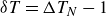 $\delta T = \Delta T_N - 1$
according to
$\delta T = \Delta T_N - 1$
according to
 \begin{equation} {Re} = \frac {{Re}^a}{\sqrt {\Delta T_N}}= \frac {{Re}^a}{\sqrt {1+ \delta T}} \sim \delta T^{-1/2} \quad \textrm {and} \quad {Nu} = \frac {{Nu}^a}{\Delta T_N} = \frac {{Nu}^a}{1 + \delta T} \sim \delta T^{-1}, \end{equation}
where the superscript
 $\Phi ^a$
denotes the achieved values by the simulation under presence of
$\Phi ^a$
denotes the achieved values by the simulation under presence of
 $\Delta T_N \neq 1$
.
$\Delta T_N \neq 1$
.
In addition to the typical definition of the global Nusselt number from (2.12) – considering the fluid domain only – one may also define a CHT Nusselt number
 $Nu_{CHT}$
which relates the heat current through the entire CHT set-up (including the solid subdomains) to the diffusive heat current through the fluid layer
$Nu_{CHT}$
which relates the heat current through the entire CHT set-up (including the solid subdomains) to the diffusive heat current through the fluid layer
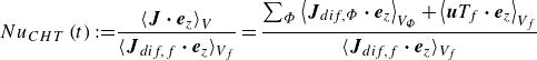 \begin{align} Nu_{CHT} \left ( t \right ) :=& \frac {\left \langle \boldsymbol{J} \boldsymbol{\cdot} \boldsymbol{e}_{z} \right \rangle _{V}}{\langle \boldsymbol{J}_{dif,f} \boldsymbol{\cdot} \boldsymbol{e}_{z} \rangle _{V_f}} = \frac {\sum _{\Phi } \left \langle \boldsymbol{J}_{dif,\Phi } \boldsymbol{\cdot} \boldsymbol{e}_{z}\right \rangle _{V_{\Phi }} + \left \langle \boldsymbol{u} T_f \boldsymbol{\cdot} \boldsymbol{e}_{z}\right \rangle _{V_{f}}}{\langle \boldsymbol{J}_{dif,f} \boldsymbol{\cdot} \boldsymbol{e}_{z} \rangle _{V_f}} \end{align}
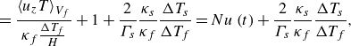 \begin{align} = \, & \frac {{\left \langle u_zT \right \rangle }_{V_f}}{\kappa _f\frac {\Delta T_f}{H}} + 1 + \frac {2}{{\Gamma _s}} \frac {\kappa _s}{\kappa _f}\frac {\Delta T_s}{\Delta T_f} = {Nu} \left (t \right )+\frac {2}{{\Gamma _s}}\frac {\kappa _s}{\kappa _f}\frac {\Delta T_s}{\Delta T_f}, \end{align}
where
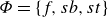 $\Phi =\{f,sb,st\}$
and
$\Phi =\{f,sb,st\}$
and
 $\Delta T_{s,f}$
are the non-dimensional temperature drops across the solid or fluid, respectively (i.e.
$\Delta T_{s,f}$
are the non-dimensional temperature drops across the solid or fluid, respectively (i.e.
 $\Delta T_f=\Delta T_N$
and
$\Delta T_f=\Delta T_N$
and
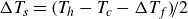 $\Delta T_s= (T_h-T_c-\Delta T_f )\!/2$
). We stress that
$\Delta T_s= (T_h-T_c-\Delta T_f )\!/2$
). We stress that
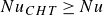 $Nu_{CHT} \geq {Nu}$
, i.e. it represents the latter plus an additional offset that vanishes for
$Nu_{CHT} \geq {Nu}$
, i.e. it represents the latter plus an additional offset that vanishes for
 $\kappa _s \! / \! \kappa _f \rightarrow \infty$
only.
$\kappa _s \! / \! \kappa _f \rightarrow \infty$
only.
Figure 6 illustrates the overall trends of the size of flow structures and their induced momentum and heat transfer for our two main series of simulations across different
 $\kappa _s \! / \! \kappa _f$
. First, see figure 6(a), we find that the qualitative impression from figure 5 is clearly supported by
$\kappa _s \! / \! \kappa _f$
. First, see figure 6(a), we find that the qualitative impression from figure 5 is clearly supported by
 $\varLambda _T ( \kappa _s \! / \! \kappa _f )$
. While such a growth of flow structures is in line with our linear stability analysis from § 3, we note that we would expect to see a further but still finite growth of turbulent flow structures for
$\varLambda _T ( \kappa _s \! / \! \kappa _f )$
. While such a growth of flow structures is in line with our linear stability analysis from § 3, we note that we would expect to see a further but still finite growth of turbulent flow structures for
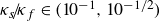 $\kappa _s \! / \! \kappa _f \in ( 10^{-1}, 10^{-1/2} )$
if we provided a sufficiently larger numerical domain.
$\kappa _s \! / \! \kappa _f \in ( 10^{-1}, 10^{-1/2} )$
if we provided a sufficiently larger numerical domain.
Size of flow structures and their induced transport. The worst solid thermal conductors (relative to the fluid) – and thus the largest flow structures – induce strongest turbulence and the greatest global heat transfer. Solid lines indicate regressions of the data points based on a hyperbolic tangent function with parameters described by table 5 . Here
 ${\Gamma _s} = 15$
for all data. Note that, in panel (d),
${\Gamma _s} = 15$
for all data. Note that, in panel (d),
 $Nu_{CHT} ( Ra = 10^{4}, \kappa _s \! / \! \kappa _f = 10^{6} ) = 2.23$
lies beyond the axis limits.
$Nu_{CHT} ( Ra = 10^{4}, \kappa _s \! / \! \kappa _f = 10^{6} ) = 2.23$
lies beyond the axis limits.
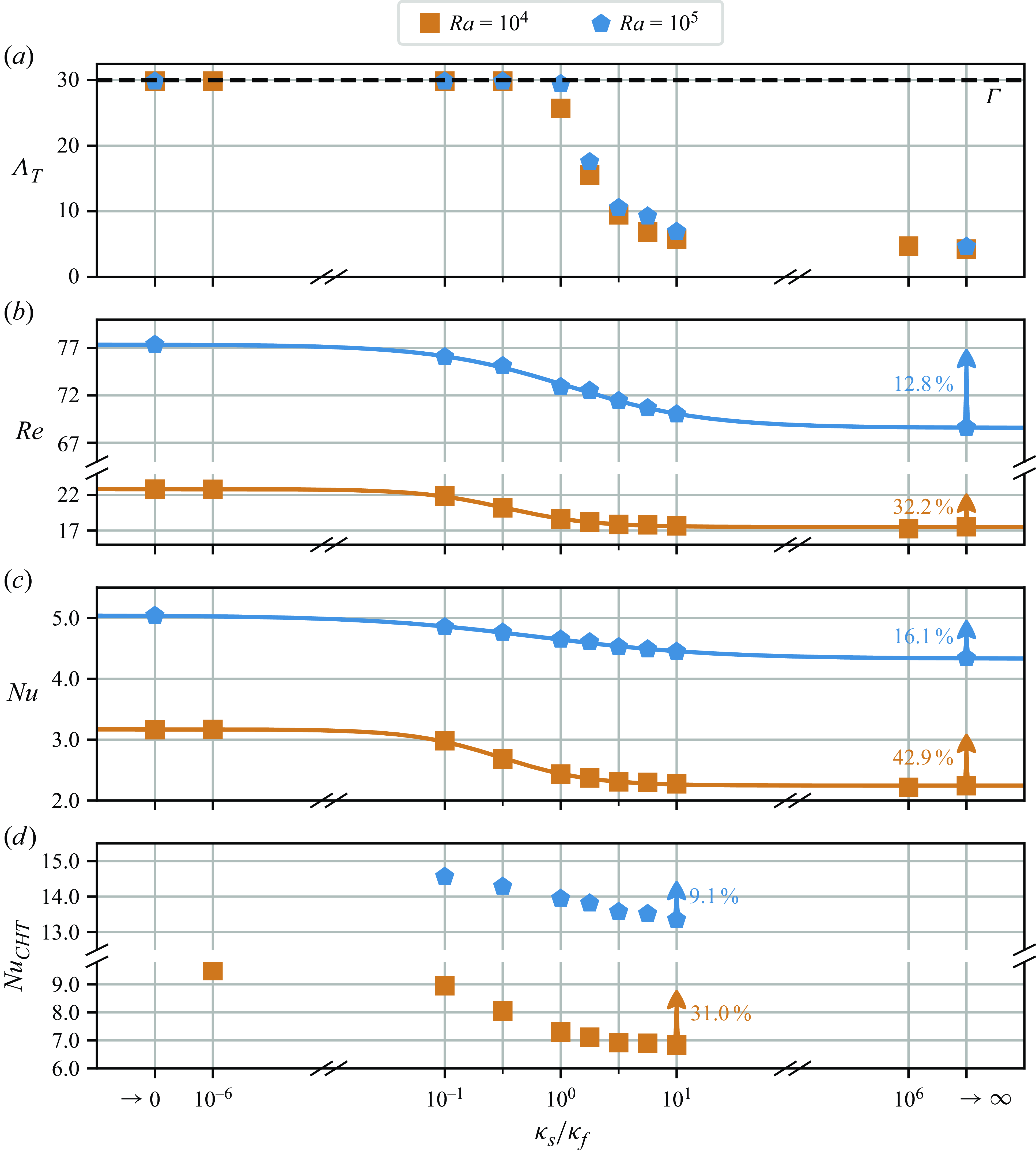
As shown by table 4, larger flow structures – or in other words, smaller
 $\kappa _s \! / \! \kappa _f$
– naturally induce stronger thermal heterogeneities at the solid–fluid interfaces. This relaxes the bounds on the temperature field (that is felt by the fluid) and allows thus for a stronger local volumetric forcing in the Navier–Stokes equation (2.2). As a result, we find an increased global transfer of momentum as shown by
$\kappa _s \! / \! \kappa _f$
– naturally induce stronger thermal heterogeneities at the solid–fluid interfaces. This relaxes the bounds on the temperature field (that is felt by the fluid) and allows thus for a stronger local volumetric forcing in the Navier–Stokes equation (2.2). As a result, we find an increased global transfer of momentum as shown by
 ${Re} ( \kappa _s \! / \! \kappa _f )$
in figure 6(b). Consequently and similarly, also the global heat transfer across the fluid layer is enhanced as measured by
${Re} ( \kappa _s \! / \! \kappa _f )$
in figure 6(b). Consequently and similarly, also the global heat transfer across the fluid layer is enhanced as measured by
 ${Nu} ( \kappa _s \! / \! \kappa _f )$
in figure 6(c). These trends are in line with previous results by Vieweg (Reference Vieweg2023) for the extreme Neumann and Dirichlet cases. In addition, see figure 6(d),
${Nu} ( \kappa _s \! / \! \kappa _f )$
in figure 6(c). These trends are in line with previous results by Vieweg (Reference Vieweg2023) for the extreme Neumann and Dirichlet cases. In addition, see figure 6(d),
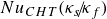 $Nu_{CHT} ( \kappa _s \! / \! \kappa _f )$
offers trends similar to
$Nu_{CHT} ( \kappa _s \! / \! \kappa _f )$
offers trends similar to
 ${Nu} ( \kappa _s \! / \! \kappa _f )$
.
${Nu} ( \kappa _s \! / \! \kappa _f )$
.
Starting from the Dirichlet- and moving towards the Neumann case, we find that both
 $Re$
and
$Re$
and
 $Nu$
experience substantial increases of up to
$Nu$
experience substantial increases of up to
 $32 \,\%$
and
$32 \,\%$
and
 $43 \,\%$
, respectively. Albeit these relative changes decrease with increasing
$43 \,\%$
, respectively. Albeit these relative changes decrease with increasing
 $Ra$
due to the increased turbulent mixing, the absolute change of
$Ra$
due to the increased turbulent mixing, the absolute change of
 $Re$
seems still to increase. This underlines that thermal boundary conditions may even affect scaling laws such as
$Re$
seems still to increase. This underlines that thermal boundary conditions may even affect scaling laws such as
 ${Nu} \sim Ra^{\gamma }$
(Plumley & Julien Reference Plumley and Julien2019; Vieweg Reference Vieweg2023) in certain ranges. In more detail, the trends in global heat transfer across the fluid layer of our three-dimensional CHT simulations in a square
${Nu} \sim Ra^{\gamma }$
(Plumley & Julien Reference Plumley and Julien2019; Vieweg Reference Vieweg2023) in certain ranges. In more detail, the trends in global heat transfer across the fluid layer of our three-dimensional CHT simulations in a square
 ${\Gamma } = 30$
domain align qualitatively with the ones of Johnston & Doering (Reference Johnston and Doering2009), the latter of which compared the Dirichlet and Neumann cases for
${\Gamma } = 30$
domain align qualitatively with the ones of Johnston & Doering (Reference Johnston and Doering2009), the latter of which compared the Dirichlet and Neumann cases for
 ${\Gamma }=2$
at
${\Gamma }=2$
at
 $Ra \leqslant 10^{10}$
in a two-dimensional domain and found that
$Ra \leqslant 10^{10}$
in a two-dimensional domain and found that
 $Nu$
is increased in the Neumann case for
$Nu$
is increased in the Neumann case for
 $Ra \lesssim 10^6$
. In contrast, the impact of the thermal boundary conditions vanished for
$Ra \lesssim 10^6$
. In contrast, the impact of the thermal boundary conditions vanished for
 $Ra \gt 10^6$
. The same trend was observed by Vieweg (Reference Vieweg2023) for three-dimensional domains of square
$Ra \gt 10^6$
. The same trend was observed by Vieweg (Reference Vieweg2023) for three-dimensional domains of square
 ${\Gamma }=60$
at
${\Gamma }=60$
at
 $Ra \lesssim 10^7$
and by Verzicco & Sreenivasan (Reference Verzicco and Sreenivasan2008) in a cylinder of
$Ra \lesssim 10^7$
and by Verzicco & Sreenivasan (Reference Verzicco and Sreenivasan2008) in a cylinder of
 ${\Gamma }=1/2$
at
${\Gamma }=1/2$
at
 $Ra \gt 10^9$
. Albeit this evidence may lead one to suspect that the impact of
$Ra \gt 10^9$
. Albeit this evidence may lead one to suspect that the impact of
 $\kappa _s \! / \! \kappa _f$
on
$\kappa _s \! / \! \kappa _f$
on
 $Nu$
and
$Nu$
and
 $Re$
vanishes for
$Re$
vanishes for
 $Ra \gg 10^5$
due to increased turbulent mixing, further studies at higher
$Ra \gg 10^5$
due to increased turbulent mixing, further studies at higher
 $Ra$
are required to prove it.
$Ra$
are required to prove it.
In analogy to § 3, we apply hyperbolic tangent fits to our numerical data. While the resulting fits are included in figure 6, their underlying parameters are provided in table 5 and allow us to estimate expected values of
 $Re$
and
$Re$
and
 $Nu$
given
$Nu$
given
 ${Pr}=1$
and
${Pr}=1$
and
 $Ra=\{10^4,10^5\}$
under different
$Ra=\{10^4,10^5\}$
under different
 $\kappa _s \! / \! \kappa _f$
. Reminiscent of § 3, we observe again an asymmetric behaviour with the inflection point being skewed towards
$\kappa _s \! / \! \kappa _f$
. Reminiscent of § 3, we observe again an asymmetric behaviour with the inflection point being skewed towards
 $\kappa _s \! / \! \kappa _f \lt 10^{0}$
.
$\kappa _s \! / \! \kappa _f \lt 10^{0}$
.
Regression parameters for
 $Nu$
and
$Nu$
and
 $Re$
. A
$Re$
. A
 $\tanh$
-fit of the form
$\tanh$
-fit of the form
 $f (\kappa _s \! / \! \kappa _f, Ra ) = a \tanh { [ b {\rm In} { ( \kappa _s \! / \! \kappa _f ) } + c ] } + d$
is applied to the values in figure 6. Here
$f (\kappa _s \! / \! \kappa _f, Ra ) = a \tanh { [ b {\rm In} { ( \kappa _s \! / \! \kappa _f ) } + c ] } + d$
is applied to the values in figure 6. Here
 $R^2$
is the coefficient of determination (Wright Reference Wright1921) and underlines the quality of these fits.
$R^2$
is the coefficient of determination (Wright Reference Wright1921) and underlines the quality of these fits.
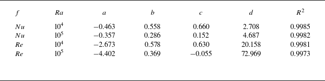
5. Boundary layer analysis
Albeit the global heat and momentum transport through the fluid layer have been quantified in § 4.3, detailed knowledge of both its thermal and viscous boundary layers is essential, too. On the one hand, the thermal boundary layers account for the majority of the temperature drop across the fluid layer (Scheel et al. Reference Scheel, Emran and Schumacher2013; Vieweg et al. Reference Vieweg, Scheel and Schumacher2021) and thus induce the essential destabilisation of the latter. On the other hand, the viscous boundary layers are highly dissipative regions (Scheel et al. Reference Scheel, Emran and Schumacher2013; Vieweg et al. Reference Vieweg, Scheel and Schumacher2021) that slow down fluid motions towards the walls and insinuate the strong turbulence present in the adjacent bulk.
While the thermal boundary layer thickness is traditionally defined based on the mean (conductive) heat transfer at the top and bottom boundaries (Chillà & Schumacher Reference Chillà and Schumacher2012)
 \begin{equation} \delta _T = \frac {1}{2 \, {Nu}} , \end{equation}
there is no equivalent transfer of momentum at these planes into the fluid. Instead, the viscous boundary layer is generated by randomly oriented patches of shear flow and usually lacks a mean flow (Samuel et al. Reference Samuel, Bode, Scheel, Sreenivasan and Schumacher2024). This structure suggests an alternative measure of the boundary layer thickness based on the full and horizontal velocity fluctuation profiles
 \begin{equation} u_{rms} \left ( z \right ) = \sqrt { \big \langle u_x^2 + u_y^2 +u_z^2 \big \rangle _{A,t}} \quad \textrm {and} \quad u_{rms}^h \left ( z \right ) = \sqrt { \big \langle u_x^2 + u_y^2 \big \rangle _{A,t}} \end{equation}
where the maxima mark the viscous fluctuation thicknesses
 $\delta _{u,rms}$
and
$\delta _{u,rms}$
and
 $\delta _{u,rms}^h$
, respectively. Equivalently, a similar definition for the thermal fluctuation thickness
$\delta _{u,rms}^h$
, respectively. Equivalently, a similar definition for the thermal fluctuation thickness
 $\delta _{\varTheta , rms}$
is given by the maximum of the temperature fluctuation profile
$\delta _{\varTheta , rms}$
is given by the maximum of the temperature fluctuation profile
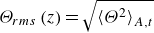 \begin{equation} \varTheta _{rms} \left ( z \right ) = \sqrt {\big \langle \varTheta ^2 \big \rangle _{A,t}} \end{equation}
which has been found to strongly correlate with
 $\delta _T$
(Long et al. Reference Long, Mound, Davies and Tobias2020). Note the difference between this profile of
$\delta _T$
(Long et al. Reference Long, Mound, Davies and Tobias2020). Note the difference between this profile of
 $\varTheta _{rms}$
and its global quantity defined in (4.2).
$\varTheta _{rms}$
and its global quantity defined in (4.2).
We prepare this analysis of thermal and viscous boundary layers by increasing the spatial resolution of our simulations: after
 $t_{r}$
(see table 3), we change the vertical number of spectral elements within the fluid layer from four to six – leading to at least
$t_{r}$
(see table 3), we change the vertical number of spectral elements within the fluid layer from four to six – leading to at least
 $14$
grid points within a boundary layer – and relax the flow onto this new grid for
$14$
grid points within a boundary layer – and relax the flow onto this new grid for
 $50 \tau _f$
before analysing the subsequent
$50 \tau _f$
before analysing the subsequent
 $100 \tau _f$
. Moreover, we rescale the temperature field for the following postprocessing based on the original
$100 \tau _f$
. Moreover, we rescale the temperature field for the following postprocessing based on the original
 $\Delta T_N$
(Vieweg Reference Vieweg2023, Reference Vieweg2024a
) for improved comparability between the Neumann and remaining cases.
$\Delta T_N$
(Vieweg Reference Vieweg2023, Reference Vieweg2024a
) for improved comparability between the Neumann and remaining cases.
Thermal boundary layer analysis. Although a glimpse at (a,d) the entire vertical profiles shows only little variation of them with
 $\kappa _s \! / \! \kappa _f$
, a closer look at the bottom region for both the planar (b,e) average and (c,f) variation reveals a more pronounced dependence of appropriately defined boundary layer thicknesses
$\kappa _s \! / \! \kappa _f$
, a closer look at the bottom region for both the planar (b,e) average and (c,f) variation reveals a more pronounced dependence of appropriately defined boundary layer thicknesses
 $\delta _{T}$
and
$\delta _{T}$
and
 $\delta _{\varTheta , rms}$
(as indicated by the horizontal lines). Note that we exploit the rescaled temperature field for this analysis and
$\delta _{\varTheta , rms}$
(as indicated by the horizontal lines). Note that we exploit the rescaled temperature field for this analysis and
 ${\Gamma _s} = 15$
for all data.
${\Gamma _s} = 15$
for all data.
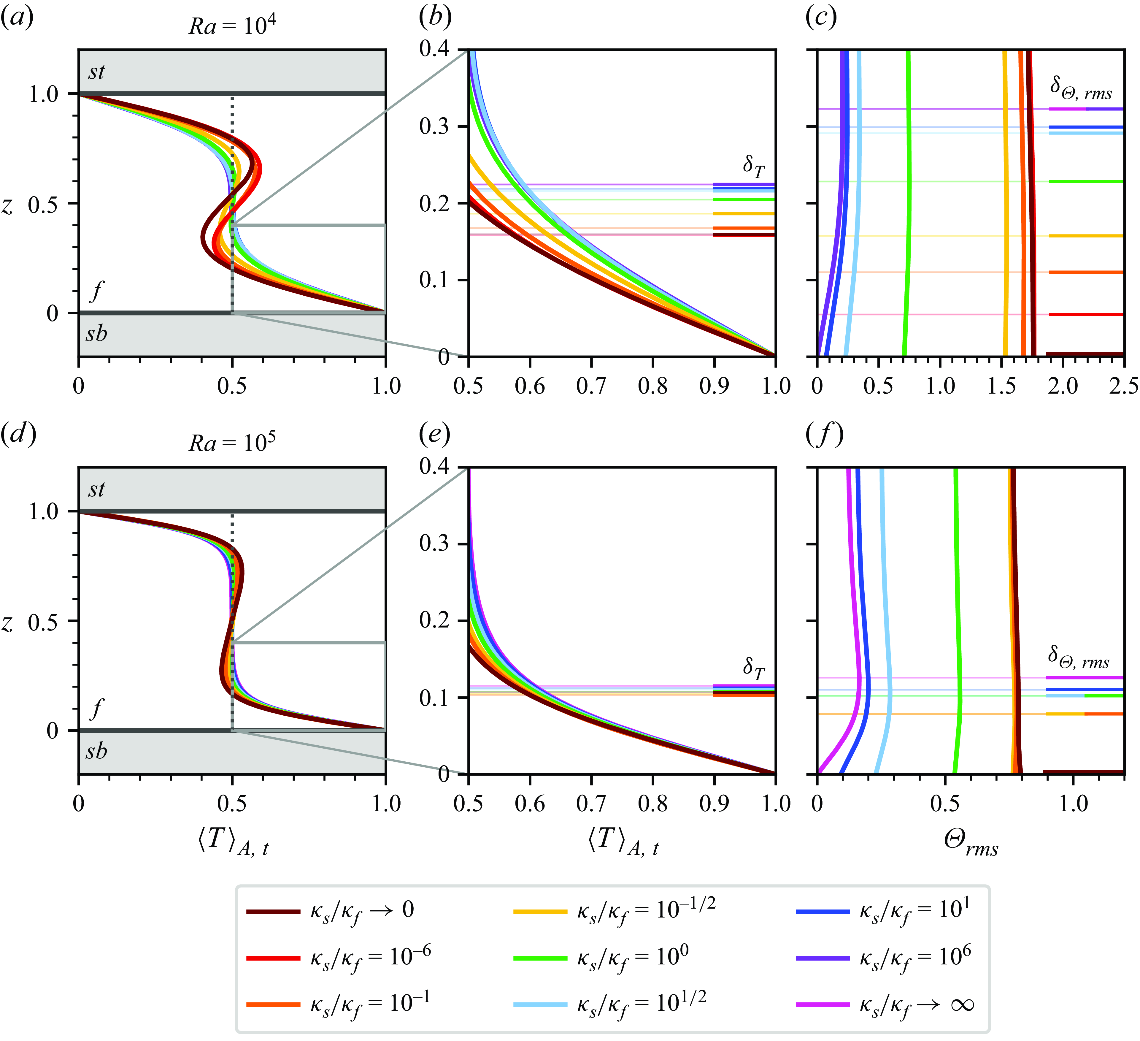
Figure 7 illustrates the mean temperature profiles across our different
 $\kappa _s \! / \! \kappa _f$
for
$\kappa _s \! / \! \kappa _f$
for
 $Ra=10^4$
in figure 7(a,b) and
$Ra=10^4$
in figure 7(a,b) and
 $Ra=10^5$
in figure 7(d,e). Bridging the gap between idealised thermal boundary conditions reported in Pandey et al. (Reference Pandey, Krasnov, Sreenivasan and Schumacher2022) and Vieweg (Reference Vieweg2023, Reference Vieweg2024a
), our CHT set-up exhibits at this intermediate
$Ra=10^5$
in figure 7(d,e). Bridging the gap between idealised thermal boundary conditions reported in Pandey et al. (Reference Pandey, Krasnov, Sreenivasan and Schumacher2022) and Vieweg (Reference Vieweg2023, Reference Vieweg2024a
), our CHT set-up exhibits at this intermediate
 ${Pr} = 1$
an increased tendency for a manifestation of a (weak) stable stratification in the bulk of the fluid layer when decreasing
${Pr} = 1$
an increased tendency for a manifestation of a (weak) stable stratification in the bulk of the fluid layer when decreasing
 $\kappa _s \! / \! \kappa _f$
. This stratification is the result of weakly mixing thermal plumes that detach and shoot deep into or even through the bulk (Vieweg Reference Vieweg2024a
). This might be supported by an increased size and thus large-scale organisation of the flow structures. As the (classical) thermal boundary layer thickness
$\kappa _s \! / \! \kappa _f$
. This stratification is the result of weakly mixing thermal plumes that detach and shoot deep into or even through the bulk (Vieweg Reference Vieweg2024a
). This might be supported by an increased size and thus large-scale organisation of the flow structures. As the (classical) thermal boundary layer thickness
 $\delta _{T}$
is directly linked to
$\delta _{T}$
is directly linked to
 $Nu$
, we find that
$Nu$
, we find that
 $\delta _{T}$
decreases with decreasing
$\delta _{T}$
decreases with decreasing
 $\kappa _s \! / \! \kappa _f$
. As
$\kappa _s \! / \! \kappa _f$
. As
 $Nu$
tends to become more independent of
$Nu$
tends to become more independent of
 $\kappa _s \! / \! \kappa _f$
for larger
$\kappa _s \! / \! \kappa _f$
for larger
 $Ra$
(see again figure 6),
$Ra$
(see again figure 6),
 $\delta _{T}$
converges as well. As an alternative to this classical measure, figure 7(c,f) visualise the thermal fluctuation thicknesses
$\delta _{T}$
converges as well. As an alternative to this classical measure, figure 7(c,f) visualise the thermal fluctuation thicknesses
 $\delta _{\varTheta , rms}$
. Given natural thermal boundary conditions that are more similar to the Dirichlet case,
$\delta _{\varTheta , rms}$
. Given natural thermal boundary conditions that are more similar to the Dirichlet case,
 $\delta _{T}$
and
$\delta _{T}$
and
 $\delta _{\varTheta , rms}$
converge as
$\delta _{\varTheta , rms}$
converge as
 $Ra$
is increased (Samuel et al. Reference Samuel, Bode, Scheel, Sreenivasan and Schumacher2024). However, for conditions more similar to the Neumann case with smaller values of
$Ra$
is increased (Samuel et al. Reference Samuel, Bode, Scheel, Sreenivasan and Schumacher2024). However, for conditions more similar to the Neumann case with smaller values of
 $\kappa _s \! / \! \kappa _f$
, the definition of
$\kappa _s \! / \! \kappa _f$
, the definition of
 $\delta _{\varTheta , rms}$
loses significance as worse solid thermal conductors imply quicker relaxations of thermal perturbations in the fluid and thus a shift of these peaks of variance closer to (or even into) the solids.
$\delta _{\varTheta , rms}$
loses significance as worse solid thermal conductors imply quicker relaxations of thermal perturbations in the fluid and thus a shift of these peaks of variance closer to (or even into) the solids.
Viscous boundary layer analysis. While in (a,d) the entire vertical profiles highlight the presence of dominant horizontally extended flow structures in particular for smaller
 $\kappa _s \! / \! \kappa _f$
and
$\kappa _s \! / \! \kappa _f$
and
 $Ra$
, these profiles’ variation allows to derive and contrast appropriately defined boundary layer thicknesses
$Ra$
, these profiles’ variation allows to derive and contrast appropriately defined boundary layer thicknesses
 $\delta _{u {, rms}}$
(as indicated by the horizontal lines) for both the full as well as only the horizontal velocity field. Note that
$\delta _{u {, rms}}$
(as indicated by the horizontal lines) for both the full as well as only the horizontal velocity field. Note that
 ${\Gamma _s} = 15$
for all data and the colour encoding coincides with figure 7.
${\Gamma _s} = 15$
for all data and the colour encoding coincides with figure 7.
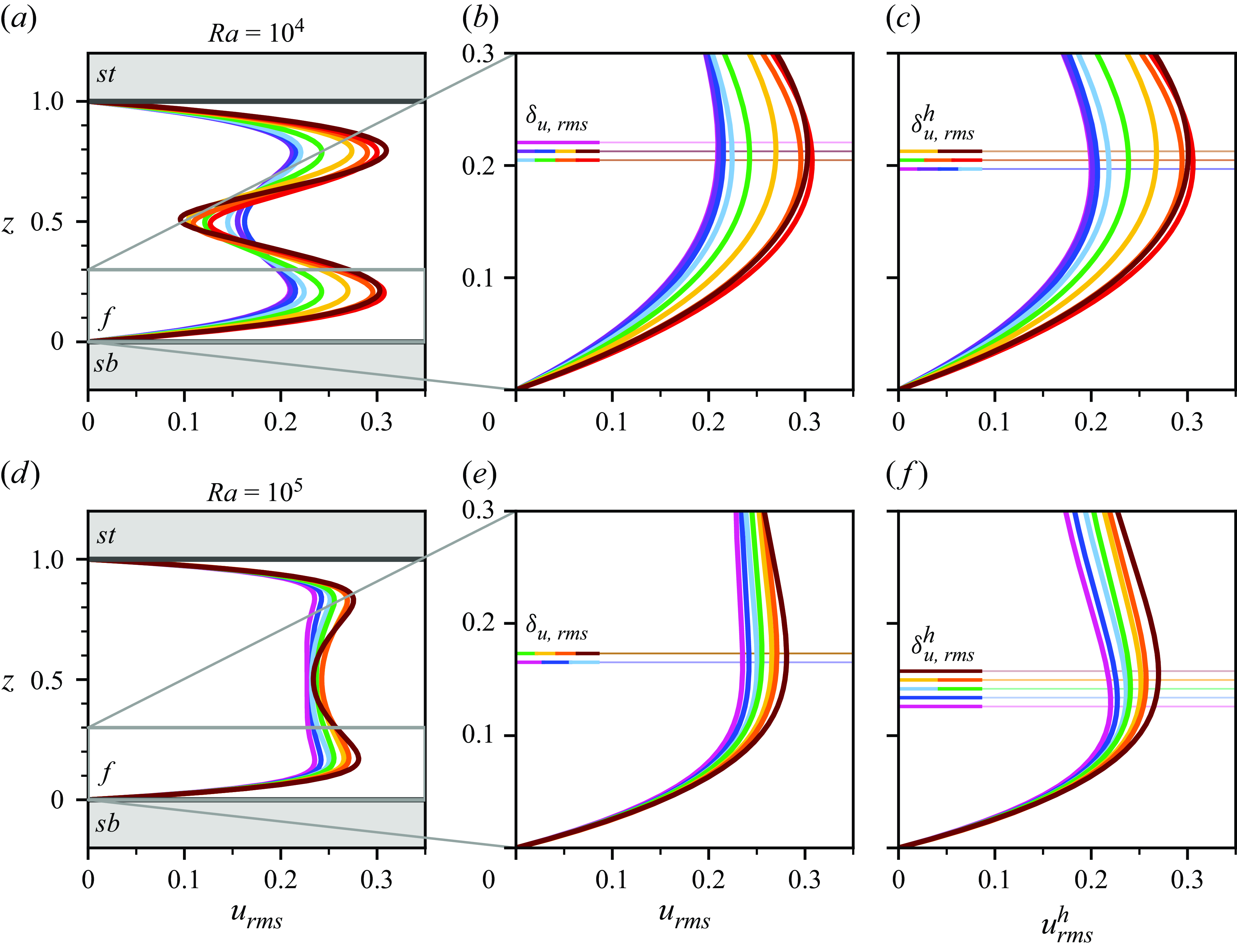
Figure 8 moves the focus of the boundary layer analysis to the velocity field. As shown across the entire fluid domain in figure 8(a,d), we observe pronounced peaks in the fluctuation profiles especially for smaller
 $\kappa _s \! / \! \kappa _f$
, i.e. for more pronounced large-scale organisations of the flow. Especially figure 8(a) indicates the presence of dominant, horizontally extended convection rolls that offer strong horizontal velocities, see also figure 8(b,c). Interestingly, despite the very different amplitudes of these profiles across
$\kappa _s \! / \! \kappa _f$
, i.e. for more pronounced large-scale organisations of the flow. Especially figure 8(a) indicates the presence of dominant, horizontally extended convection rolls that offer strong horizontal velocities, see also figure 8(b,c). Interestingly, despite the very different amplitudes of these profiles across
 $\kappa _s \! / \! \kappa _f$
, the viscous boundary layer thickness is very similar and varies only weakly with
$\kappa _s \! / \! \kappa _f$
, the viscous boundary layer thickness is very similar and varies only weakly with
 $Ra$
(and thus
$Ra$
(and thus
 $Re$
). In other words, the viscous boundary layer thickness varies less with both
$Re$
). In other words, the viscous boundary layer thickness varies less with both
 $\kappa _s \! / \! \kappa _f$
and
$\kappa _s \! / \! \kappa _f$
and
 $Ra$
than the thermal one. As a result, the ratio
$Ra$
than the thermal one. As a result, the ratio
 $\delta _{u,rms}/\delta _{\varTheta ,rms}$
tends to increase for larger
$\delta _{u,rms}/\delta _{\varTheta ,rms}$
tends to increase for larger
 $Ra$
(Samuel et al. Reference Samuel, Bode, Scheel, Sreenivasan and Schumacher2024). However, our data suggests that it is not solely
$Ra$
(Samuel et al. Reference Samuel, Bode, Scheel, Sreenivasan and Schumacher2024). However, our data suggests that it is not solely
 $Re$
that governs the thickness of the viscous boundary layer: for fixed
$Re$
that governs the thickness of the viscous boundary layer: for fixed
 $Ra$
, our
$Ra$
, our
 $Re$
is larger for smaller
$Re$
is larger for smaller
 $\kappa _s \! / \! \kappa _f$
even though both
$\kappa _s \! / \! \kappa _f$
even though both
 $\delta _{u,rms}$
and
$\delta _{u,rms}$
and
 $\delta _{u,rms}^h$
exhibit the opposite trend. This suggests that long-living large-scale flow structures play a crucial role even for viscous boundary layers.
$\delta _{u,rms}^h$
exhibit the opposite trend. This suggests that long-living large-scale flow structures play a crucial role even for viscous boundary layers.
6. The impact of the plate thickness
6.1. Choice of the vertical aspect ratio
$\Gamma _s$

In all our simulations discussed so far, a vertical aspect ratio of
 ${\Gamma _s}=15$
has been used. This deliberate choice is based on a diffusion time argument: temperature differences are supposed to relax more quickly in the horizontal than in vertical direction,
${\Gamma _s}=15$
has been used. This deliberate choice is based on a diffusion time argument: temperature differences are supposed to relax more quickly in the horizontal than in vertical direction,
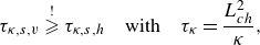 \begin{equation} \tau _{\kappa ,s,v}\stackrel {!}{\geqslant }\tau _{\kappa ,s,h} \quad \textrm {with} \quad \tau _{\kappa }=\frac {L_{ch}^2}{\kappa } , \end{equation}
promoting a weak to negligible footprint of the applied thermal boundary conditions on the solid–fluid interfaces. Given our laterally periodic domain, the largest structure satisfying this condition has a horizontal extend of
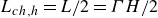 $L_{ch,h}=L/2={\Gamma } H/2$
. Hence, condition (6.1) turns into
$L_{ch,h}=L/2={\Gamma } H/2$
. Hence, condition (6.1) turns into
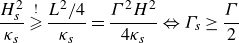 \begin{equation} \frac {H_s^2}{\kappa _s} \stackrel {!}{\geqslant } \frac {L^2/4}{\kappa _s} = \frac {{\Gamma }^2H^2}{4\kappa _s} \Leftrightarrow {\Gamma _s} \geq \frac {{\Gamma }}{2} \end{equation}
and a domain of
 ${\Gamma }=30$
should offer (at least)
${\Gamma }=30$
should offer (at least)
 ${\Gamma _s}=15$
.
${\Gamma _s}=15$
.
Relaxation of turbulent flow-induced thermal perturbations across the solid plates. (a) Given
 ${\Gamma _s} = 15$
(at
${\Gamma _s} = 15$
(at
 $Ra = 10^{5}$
), the relaxation is slowest close to a unity ratio
$Ra = 10^{5}$
), the relaxation is slowest close to a unity ratio
 $\kappa _s \! / \! \kappa _f = 10^{0}$
. Even for this critical case, (b) the situation has mostly converged to that with plates of even twice the thickness. In contrast, thinner plates with
$\kappa _s \! / \! \kappa _f = 10^{0}$
. Even for this critical case, (b) the situation has mostly converged to that with plates of even twice the thickness. In contrast, thinner plates with
 ${\Gamma _s} = 1$
impact the temperature field at the solid–fluid interfaces strongly. The situation is symmetric for
${\Gamma _s} = 1$
impact the temperature field at the solid–fluid interfaces strongly. The situation is symmetric for
 $- {\Gamma _s} \leq z \leq 0$
.
$- {\Gamma _s} \leq z \leq 0$
.
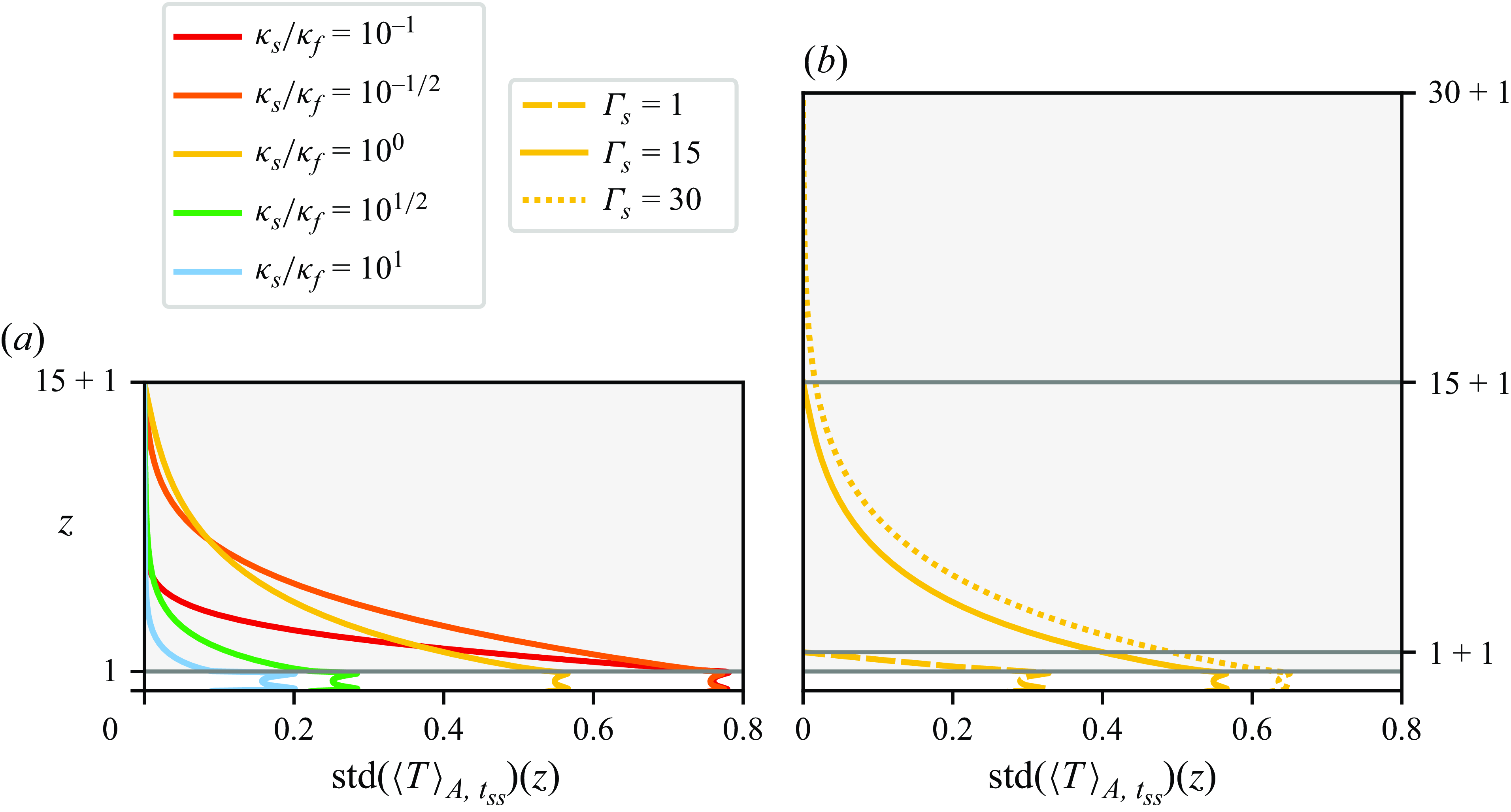
Figure 9 scrutinises our condition (6.2) by plotting and contrasting vertical profiles of the standard deviation in the temperature field
 $\mathrm{std} ( T )$
across all
$\mathrm{std} ( T )$
across all
 $\kappa _s \! / \! \kappa _f$
in figure 9(a). We find that the propagation of thermal inhomogeneities into the solid plates is asymmetric with respect to
$\kappa _s \! / \! \kappa _f$
in figure 9(a). We find that the propagation of thermal inhomogeneities into the solid plates is asymmetric with respect to
 $\kappa _s \! / \! \kappa _f$
. Interestingly, thermal perturbations relax most slowly in case of
$\kappa _s \! / \! \kappa _f$
. Interestingly, thermal perturbations relax most slowly in case of
 $\kappa _s \! / \! \kappa _f = 10^{0}$
despite its weaker thermal inhomogeneities at the solid–fluid interface compared with
$\kappa _s \! / \! \kappa _f = 10^{0}$
despite its weaker thermal inhomogeneities at the solid–fluid interface compared with
 $\kappa _s \! / \! \kappa _f = \left \{ 10^{-1}, 10^{-1/2} \right \}$
(see also again table 4).
$\kappa _s \! / \! \kappa _f = \left \{ 10^{-1}, 10^{-1/2} \right \}$
(see also again table 4).
In order to probe the impact of our applied thermal boundary condition at
 $z = 1 + {\Gamma _s}$
(see (2.9)), we proceed by varying
$z = 1 + {\Gamma _s}$
(see (2.9)), we proceed by varying
 $\Gamma _s$
given a fixed
$\Gamma _s$
given a fixed
 $\kappa _s \! / \! \kappa _f = 10^{0}$
. Figure 9(b) contrasts two additional simulations of
$\kappa _s \! / \! \kappa _f = 10^{0}$
. Figure 9(b) contrasts two additional simulations of
 ${\Gamma _s} = \left \{ 1, 30 \right \}$
with the previous case. On the one hand, we find that thin plates of
${\Gamma _s} = \left \{ 1, 30 \right \}$
with the previous case. On the one hand, we find that thin plates of
 ${\Gamma _s}=1$
result in significant decreases of the thermal inhomogeneities and size of the resulting flow structures compared with
${\Gamma _s}=1$
result in significant decreases of the thermal inhomogeneities and size of the resulting flow structures compared with
 ${\Gamma _s} = 15$
, see also again table 4. This suggests that temperature differences in the horizontal direction are not sufficiently relaxed and that the underlying thermal boundary conditions leave a considerable footprint on the solid–fluid interfaces. On the other hand, even thicker plates of
${\Gamma _s} = 15$
, see also again table 4. This suggests that temperature differences in the horizontal direction are not sufficiently relaxed and that the underlying thermal boundary conditions leave a considerable footprint on the solid–fluid interfaces. On the other hand, even thicker plates of
 ${\Gamma _s}=30$
do not seem to provide a significant benefit. Despite somewhat larger inhomogeneities at the solid–fluid interfaces, the vertical profile underlines that the relaxation of thermal inhomogeneity is barely altered despite a doubling of the plate thickness. Hence, we conclude that the choice of
${\Gamma _s}=30$
do not seem to provide a significant benefit. Despite somewhat larger inhomogeneities at the solid–fluid interfaces, the vertical profile underlines that the relaxation of thermal inhomogeneity is barely altered despite a doubling of the plate thickness. Hence, we conclude that the choice of
 ${\Gamma _s} = 15$
based on condition (6.2) for our main production simulations has been appropriate.
${\Gamma _s} = 15$
based on condition (6.2) for our main production simulations has been appropriate.
6.2. Linear stability analysis for different plate thicknesses
$\Gamma _s$

Similar to the turbulent flow at
 $Ra \gg Ra_{c}$
, we expect the onset of convection to be affected by the thickness of the solid plates
$Ra \gg Ra_{c}$
, we expect the onset of convection to be affected by the thickness of the solid plates
 $\Gamma _s$
. As shown in Appendix A, we extend the work of Hurle et al. (Reference Hurle, Jakeman and Pike1967) (who considered
$\Gamma _s$
. As shown in Appendix A, we extend the work of Hurle et al. (Reference Hurle, Jakeman and Pike1967) (who considered
 ${\Gamma _s} \rightarrow \infty$
) by respecting the plate thickness via the
${\Gamma _s} \rightarrow \infty$
) by respecting the plate thickness via the
 $-\lambda _f \! / \! \lambda _s \tanh (k {\Gamma _s} )$
term in the solution of the linear stability of the system (see (3.1)).
$-\lambda _f \! / \! \lambda _s \tanh (k {\Gamma _s} )$
term in the solution of the linear stability of the system (see (3.1)).
Figure 10 compares various neutral stability curves given constant
 $\lambda _s \! / \! \lambda _f$
in different panels. On the one hand, we find that the curves (across the different panels) converge for infinitely small vertical aspect ratios
$\lambda _s \! / \! \lambda _f$
in different panels. On the one hand, we find that the curves (across the different panels) converge for infinitely small vertical aspect ratios
 ${\Gamma _s} \rightarrow 0$
– independently of
${\Gamma _s} \rightarrow 0$
– independently of
 $\lambda _s \! / \! \lambda _f$
– towards the classical Dirichlet case (i.e. the violet curves are all the same). This case, making any plates obsolete, is certainly influenced by our applied Dirichlet-type boundary conditions at the very top and bottom. On the other hand, we observe that the curves (in each panel) converge for large vertical aspect ratios
$\lambda _s \! / \! \lambda _f$
– towards the classical Dirichlet case (i.e. the violet curves are all the same). This case, making any plates obsolete, is certainly influenced by our applied Dirichlet-type boundary conditions at the very top and bottom. On the other hand, we observe that the curves (in each panel) converge for large vertical aspect ratios
 ${\Gamma _s} \gg 1$
independently of
${\Gamma _s} \gg 1$
independently of
 $\lambda _s \! / \! \lambda _f$
. In other words, there is practically no difference between
$\lambda _s \! / \! \lambda _f$
. In other words, there is practically no difference between
 ${\Gamma _s}=15$
and
${\Gamma _s}=15$
and
 ${\Gamma _s} \rightarrow \infty$
. This substantiates our choice of
${\Gamma _s} \rightarrow \infty$
. This substantiates our choice of
 ${\Gamma _s}=15$
in § 6.1. Additionally, we find that the neutral stability curves converge for
${\Gamma _s}=15$
in § 6.1. Additionally, we find that the neutral stability curves converge for
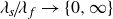 $\lambda _s \! / \! \lambda _f \rightarrow \left \{ 0, \infty \right \}$
as long as
$\lambda _s \! / \! \lambda _f \rightarrow \left \{ 0, \infty \right \}$
as long as
 ${\Gamma _s} \gt 0$
and sufficiently large (e.g.
${\Gamma _s} \gt 0$
and sufficiently large (e.g.
 ${\Gamma _s} = 0.1$
). Only a zoom towards
${\Gamma _s} = 0.1$
). Only a zoom towards
 $k \approx 0$
, see figure 10(d), indicates the gradual convergence of the critical wavenumber for the Neumann case as one of these two idealised thermal boundary conditions. For such small, yet positive
$k \approx 0$
, see figure 10(d), indicates the gradual convergence of the critical wavenumber for the Neumann case as one of these two idealised thermal boundary conditions. For such small, yet positive
 $\lambda _s \! / \! \lambda _f$
, the solid plates conduct heat way worse than the fluid, and so even very thin plates of
$\lambda _s \! / \! \lambda _f$
, the solid plates conduct heat way worse than the fluid, and so even very thin plates of
 ${\Gamma _s}=0.1$
effectively act insulating. This may have important implications for any coating of a wall in laboratory convection set-ups (Schindler et al. Reference Schindler, Eckert, Zürner, Schumacher and Vogt2022, Reference Schindler, Eckert, Zürner, Schumacher and Vogt2023; Wondrak et al. Reference Wondrak, Sieger, Mitra, Schindler, Stefani, Vogt and Eckert2023).
${\Gamma _s}=0.1$
effectively act insulating. This may have important implications for any coating of a wall in laboratory convection set-ups (Schindler et al. Reference Schindler, Eckert, Zürner, Schumacher and Vogt2022, Reference Schindler, Eckert, Zürner, Schumacher and Vogt2023; Wondrak et al. Reference Wondrak, Sieger, Mitra, Schindler, Stefani, Vogt and Eckert2023).
The situation becomes significantly more complex once no limit of either
 $\Gamma _s$
or
$\Gamma _s$
or
 $\lambda _s \! / \! \lambda _f$
is considered. Contrasting figure 10(b,c,e,f), a certain asymmetry around
$\lambda _s \! / \! \lambda _f$
is considered. Contrasting figure 10(b,c,e,f), a certain asymmetry around
 $\lambda _s \! / \! \lambda _f=10^0$
can (once again) be noticed. While the neutral stability curves almost coincide for
$\lambda _s \! / \! \lambda _f=10^0$
can (once again) be noticed. While the neutral stability curves almost coincide for
 $\lambda _s \! / \! \lambda _f=10^1$
in figure 10(f), there is a significant spread for
$\lambda _s \! / \! \lambda _f=10^1$
in figure 10(f), there is a significant spread for
 $\lambda _s \! / \! \lambda _f=10^{-1}$
in figure 10(c). This begs the following question: Which ratio of thermal conductivities is most sensitive to a variation of
$\lambda _s \! / \! \lambda _f=10^{-1}$
in figure 10(c). This begs the following question: Which ratio of thermal conductivities is most sensitive to a variation of
 ${\Gamma _s}?$
Neutral stability across varying
 $\Gamma _s$
. While vertically infinitely extended plates are already resembled at
$\Gamma _s$
. While vertically infinitely extended plates are already resembled at
 ${\Gamma _s} \gg 1$
, thinner plates
${\Gamma _s} \gg 1$
, thinner plates
 ${\Gamma _s} \lesssim 1$
impact the system significantly and stabilise the layer successively. Worse solid thermal conductors (relative to the fluid) are more strongly affected by this stabilisation; contrast therefore in particular panels (c,f) which are symmetrically spaced around
${\Gamma _s} \lesssim 1$
impact the system significantly and stabilise the layer successively. Worse solid thermal conductors (relative to the fluid) are more strongly affected by this stabilisation; contrast therefore in particular panels (c,f) which are symmetrically spaced around
 $\lambda _s \! / \! \lambda _f = 10^{0}$
.
$\lambda _s \! / \! \lambda _f = 10^{0}$
.
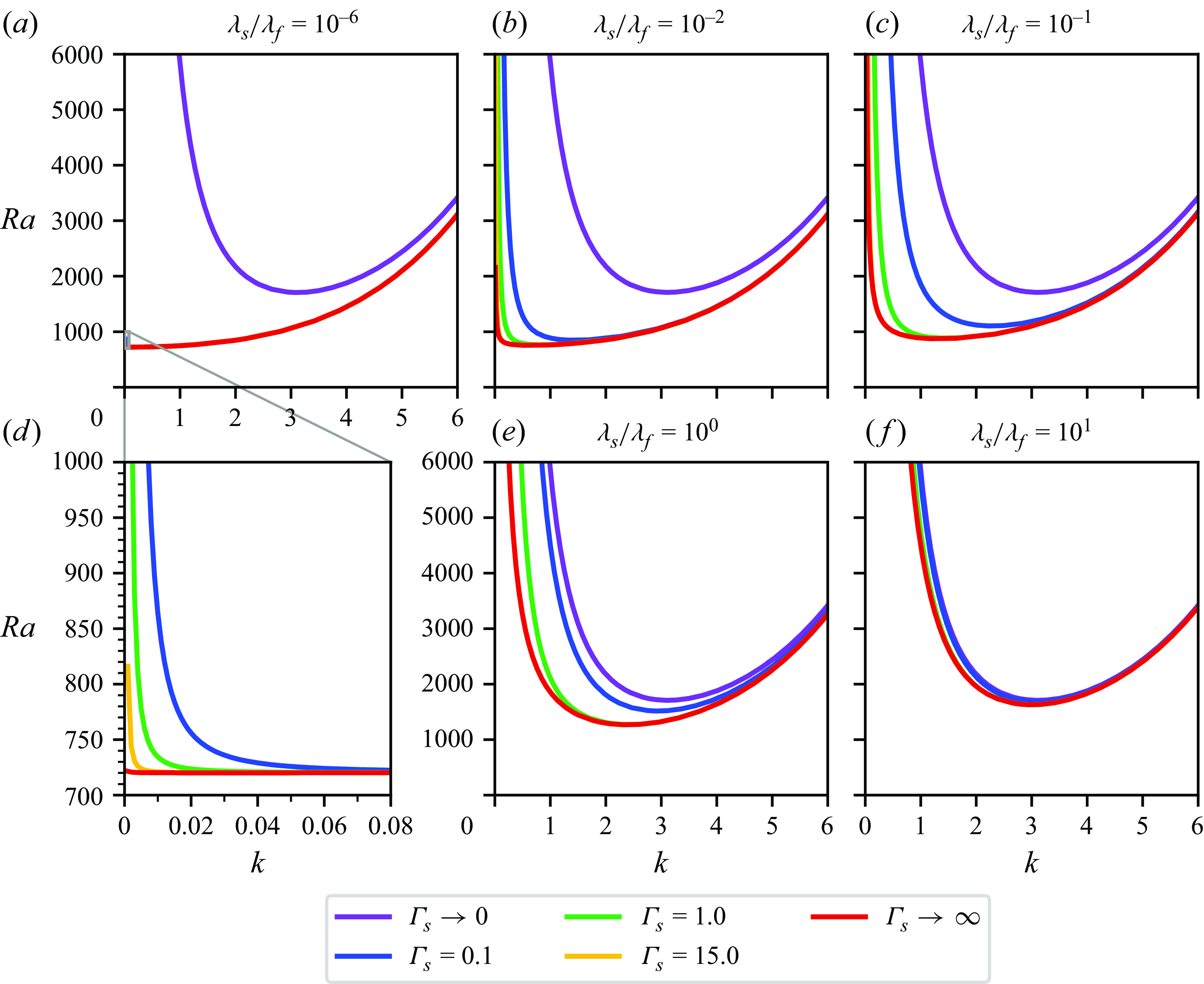
Sensitivity of neutral stability on plate thickness for varying
 $\lambda _s \! / \! \lambda _f$
. The differences in
$\lambda _s \! / \! \lambda _f$
. The differences in
 $Ra_{c}$
(a) and corresponding
$Ra_{c}$
(a) and corresponding
 $k_{c}$
(b) are shown when moving from infinitely thick (
$k_{c}$
(b) are shown when moving from infinitely thick (
 ${\Gamma _s}\rightarrow \infty$
) towards very thin plates (
${\Gamma _s}\rightarrow \infty$
) towards very thin plates (
 ${\Gamma _s}=0.1$
). Decreasing
${\Gamma _s}=0.1$
). Decreasing
 $\Gamma _s$
thus stabilises the layer successively, with the strongest impact near
$\Gamma _s$
thus stabilises the layer successively, with the strongest impact near
 $\lambda _s \! / \! \lambda _f\approx 10^{-1/2}$
, not just shifting the onset of convection, but also reducing the initial pattern size at this point.
$\lambda _s \! / \! \lambda _f\approx 10^{-1/2}$
, not just shifting the onset of convection, but also reducing the initial pattern size at this point.
In an attempt to quantify the divergence of the neutral stability curves, we measure the differences in
 $Ra_{c}$
and
$Ra_{c}$
and
 $k_{c}$
between the cases of
$k_{c}$
between the cases of
 ${\Gamma _s} = 0.1$
and
${\Gamma _s} = 0.1$
and
 ${\Gamma _s}\rightarrow \infty$
via
${\Gamma _s}\rightarrow \infty$
via
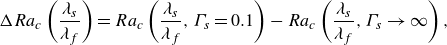 \begin{align}&\qquad \Delta Ra_{c} \left ( \frac {\lambda _s}{\lambda _f} \right ) = Ra_{c} \left ( \frac {\lambda _s}{\lambda _f}, {\Gamma _s}=0.1 \right ) - Ra_{c} \left ( \frac {\lambda _s}{\lambda _f}, {\Gamma _s} \rightarrow \infty \right ), \end{align}
 \begin{align}& \Delta k_{c} \left ( \frac {\lambda _s}{\lambda _f} \right ) = k_{c} \left ( Ra_{c} \left ( \frac {\lambda _s}{\lambda _f}, {\Gamma _s}=0.1 \right ) \right ) - k_{c} \left ( Ra_{c} \left ( \frac {\lambda _s}{\lambda _f}, {\Gamma _s} \rightarrow \infty \right ) \right ). \end{align}
Figure 11 illustrates these results. Note that while
 $\Delta Ra_{c} \gt 0$
implies a stabilisation of the convection layer when decreasing the thickness of the solid plates,
$\Delta Ra_{c} \gt 0$
implies a stabilisation of the convection layer when decreasing the thickness of the solid plates,
 $\Delta k_{c} \gt 0$
indicates a decrease in the size of critical flow structures. Moreover, we find that both
$\Delta k_{c} \gt 0$
indicates a decrease in the size of critical flow structures. Moreover, we find that both
 $\Delta Ra_{c}$
and
$\Delta Ra_{c}$
and
 $\Delta k_{c}$
offer pronounced peaks around
$\Delta k_{c}$
offer pronounced peaks around
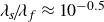 $\lambda _s \! / \! \lambda _f \approx 10^{-0.5}$
and
$\lambda _s \! / \! \lambda _f \approx 10^{-0.5}$
and
 $\lambda _s \! / \! \lambda _f \approx 10^{-1}$
, respectively. Supported by the general asymmetry of these curves, this analysis underlines the complex ramifications an interplay between the solid and fluid domain can exhibit.
$\lambda _s \! / \! \lambda _f \approx 10^{-1}$
, respectively. Supported by the general asymmetry of these curves, this analysis underlines the complex ramifications an interplay between the solid and fluid domain can exhibit.
7. Discussion and perspective
Long-living large-scale flow structures are crucial for an understanding and prediction of convection flows such as in the Earth’s atmosphere. Previous studies of horizontally extended Rayleigh–Bénard convection focussed on idealised thermal boundary conditions such as constant temperatures (the so-called Dirichlet case) or a constant heat flux (Neumann case) (Pandey et al. Reference Pandey, Scheel and Schumacher2018; Vieweg et al. Reference Vieweg, Scheel and Schumacher2021; Vieweg Reference Vieweg2023). However, these conditions reduce the problem to the fluid layer only and thus represent rather idealised cases. In contrast, any natural convection flow is confined by some adjacent matter. Using a coupled or CHT set-up, this study includes two identical fluid-confining solid plates at the bottom and the top of the fluid layer. The ratio of thermal diffusivities
 $\kappa _s \! / \! \kappa _f$
between the solids and the fluid represents the key control parameter characterising the (to the perspective of the fluid) resulting thermal boundary conditions. The inclusion of solid subdomains allows us to resemble the Neumann case via
$\kappa _s \! / \! \kappa _f$
between the solids and the fluid represents the key control parameter characterising the (to the perspective of the fluid) resulting thermal boundary conditions. The inclusion of solid subdomains allows us to resemble the Neumann case via
 $\kappa _s \! / \! \kappa _f \rightarrow 0$
and the Dirichlet case via
$\kappa _s \! / \! \kappa _f \rightarrow 0$
and the Dirichlet case via
 $\kappa _s \! / \! \kappa _f \rightarrow \infty$
, see Appendix B. Varying
$\kappa _s \! / \! \kappa _f \rightarrow \infty$
, see Appendix B. Varying
 $\kappa _s \! / \! \kappa _f$
across a broad range, this study bridges the gap in between by introducing natural thermal boundary conditions.
$\kappa _s \! / \! \kappa _f$
across a broad range, this study bridges the gap in between by introducing natural thermal boundary conditions.
Given a Prandtl number
 ${Pr}=1$
, (horizontal) aspect ratio
${Pr}=1$
, (horizontal) aspect ratio
 ${\Gamma }=30$
and thickness of the solid plates
${\Gamma }=30$
and thickness of the solid plates
 ${\Gamma _s}=15$
, we have conducted direct numerical simulations subject to varying
${\Gamma _s}=15$
, we have conducted direct numerical simulations subject to varying
 $\kappa _s \! / \! \kappa _f$
for
$\kappa _s \! / \! \kappa _f$
for
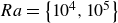 $Ra= \left \{10^4, 10^5 \right \}$
under no-slip boundary conditions at the solid–fluid interfaces and periodic boundary conditions concerning the lateral extent of the domain of square horizontal cross-section. As shown in figure 4, such a coupled system allows for highly complex dynamics of both
$Ra= \left \{10^4, 10^5 \right \}$
under no-slip boundary conditions at the solid–fluid interfaces and periodic boundary conditions concerning the lateral extent of the domain of square horizontal cross-section. As shown in figure 4, such a coupled system allows for highly complex dynamics of both
 $T$
and
$T$
and
 $\partial T / \partial z$
at the various (partly solid–fluid) interfaces based on the manifesting fluid flow.
$\partial T / \partial z$
at the various (partly solid–fluid) interfaces based on the manifesting fluid flow.
Varying
 $\kappa _s \! / \! \kappa _f$
from
$\kappa _s \! / \! \kappa _f$
from
 $\kappa _s \! / \! \kappa _f \gg 10^{0}$
towards
$\kappa _s \! / \! \kappa _f \gg 10^{0}$
towards
 $\kappa _s \! / \! \kappa _f \ll 10^{0}$
, we found that both structural as well as statistical properties of the flow undergo significant changes: the long-living large-scale flow structures grow, and both their induced momentum and heat transfer are (asymmetrically with respect to
$\kappa _s \! / \! \kappa _f \ll 10^{0}$
, we found that both structural as well as statistical properties of the flow undergo significant changes: the long-living large-scale flow structures grow, and both their induced momentum and heat transfer are (asymmetrically with respect to
 $\kappa _s \! / \! \kappa _f$
) increased by up to
$\kappa _s \! / \! \kappa _f$
) increased by up to
 $43 \,\%$
. The increase of these measures can be explained by stronger thermal inhomogeneities – the footprints of these flow structures – at the solid–fluid interfaces and align with recent results for idealised thermal boundary conditions (Vieweg et al. Reference Vieweg, Scheel and Schumacher2021; Vieweg Reference Vieweg2023) or strongly asymmetric CHT set-ups (Vieweg et al. Reference Vieweg, Käufer, Cierpka and Schumacher2025). We observe a gradual transition from turbulent superstructures towards supergranules, underlining the importance of the umbrella term of long-living large-scale flow structures (Vieweg Reference Vieweg2023).
$43 \,\%$
. The increase of these measures can be explained by stronger thermal inhomogeneities – the footprints of these flow structures – at the solid–fluid interfaces and align with recent results for idealised thermal boundary conditions (Vieweg et al. Reference Vieweg, Scheel and Schumacher2021; Vieweg Reference Vieweg2023) or strongly asymmetric CHT set-ups (Vieweg et al. Reference Vieweg, Käufer, Cierpka and Schumacher2025). We observe a gradual transition from turbulent superstructures towards supergranules, underlining the importance of the umbrella term of long-living large-scale flow structures (Vieweg Reference Vieweg2023).
A linear stability analysis of our CHT set-up confirms both the growth of flow structures as well as an increased heat transfer for smaller values of
 $\lambda _s \! / \! \lambda _f$
. In other words, we observe a monotonic shift of both the critical Rayleigh number
$\lambda _s \! / \! \lambda _f$
. In other words, we observe a monotonic shift of both the critical Rayleigh number
 $Ra_{c}$
and critical wavenumber
$Ra_{c}$
and critical wavenumber
 $k_{c}$
when varying
$k_{c}$
when varying
 $\lambda _s \! / \! \lambda _f$
between its limits. This implies a change in the supercriticality
$\lambda _s \! / \! \lambda _f$
between its limits. This implies a change in the supercriticality
 $Ra / Ra_{c}$
given a fixed
$Ra / Ra_{c}$
given a fixed
 $Ra \gt Ra_{c}$
and affects thus the induced heat transfer.
$Ra \gt Ra_{c}$
and affects thus the induced heat transfer.
We have extended the previous work by Hurle et al. (Reference Hurle, Jakeman and Pike1967) with respect to two important aspects: first, we provided simple relations or regressions for
 $k_{c} ( \lambda _s \! / \! \lambda _f )$
,
$k_{c} ( \lambda _s \! / \! \lambda _f )$
,
 $Ra_{c} ( \lambda _s \! / \! \lambda _f )$
, and
$Ra_{c} ( \lambda _s \! / \! \lambda _f )$
, and
 $Ra_{c} ( k_{c} )$
– see again table 2. This hopefully improves the accessibility of our results. Second, we investigated the impact of a finite thickness of the solid plates in § 6.2, allowing us to understand the convergence of the system for the limits
$Ra_{c} ( k_{c} )$
– see again table 2. This hopefully improves the accessibility of our results. Second, we investigated the impact of a finite thickness of the solid plates in § 6.2, allowing us to understand the convergence of the system for the limits
 $\left \{ {\Gamma _s}, \lambda _s \! / \! \lambda _f \right \} \rightarrow \left \{ 0, \infty \right \}$
and find its point of largest susceptibility to a change in the plate thickness (as quantified by
$\left \{ {\Gamma _s}, \lambda _s \! / \! \lambda _f \right \} \rightarrow \left \{ 0, \infty \right \}$
and find its point of largest susceptibility to a change in the plate thickness (as quantified by
 $\Delta Ra_{c}$
) at
$\Delta Ra_{c}$
) at
 $\lambda _s \! / \! \lambda _f \approx 10^{-1/2}$
.
$\lambda _s \! / \! \lambda _f \approx 10^{-1/2}$
.
This effect of a varying plate thickness
 $\Gamma _s$
was additionally studied numerically. We found that
$\Gamma _s$
was additionally studied numerically. We found that
 ${\Gamma _s} \lesssim 1$
tends to stamp the external thermal boundary condition onto the internal solid–fluid interface, whereas our chosen
${\Gamma _s} \lesssim 1$
tends to stamp the external thermal boundary condition onto the internal solid–fluid interface, whereas our chosen
 ${\Gamma _s} = 15 \gg 1$
represents a fair approximation of
${\Gamma _s} = 15 \gg 1$
represents a fair approximation of
 ${\Gamma _s} \rightarrow \infty$
. We note at this point that the computational cost of one CHT simulation involving
${\Gamma _s} \rightarrow \infty$
. We note at this point that the computational cost of one CHT simulation involving
 ${\Gamma _s} = 15$
increases the required wallclock solution time by a factor of roughly
${\Gamma _s} = 15$
increases the required wallclock solution time by a factor of roughly
 $8$
compared with a simulation without solid plates (for the same number of non-dimensional time units
$8$
compared with a simulation without solid plates (for the same number of non-dimensional time units
 $\tau _f$
). Both this numerical investigation of varying
$\tau _f$
). Both this numerical investigation of varying
 $\Gamma _s$
as well as the corresponding investigation of the linear stability have important implications for the design of laboratory experiments (Foroozani et al. Reference Foroozani, Krasnov and Schumacher2021; Moller, Resagk & Cierpka Reference Moller, Resagk and Cierpka2021; Moller Reference Moller2022; Wondrak et al. Reference Wondrak, Sieger, Mitra, Schindler, Stefani, Vogt and Eckert2023; Vieweg et al. Reference Vieweg, Käufer, Cierpka and Schumacher2025).
$\Gamma _s$
as well as the corresponding investigation of the linear stability have important implications for the design of laboratory experiments (Foroozani et al. Reference Foroozani, Krasnov and Schumacher2021; Moller, Resagk & Cierpka Reference Moller, Resagk and Cierpka2021; Moller Reference Moller2022; Wondrak et al. Reference Wondrak, Sieger, Mitra, Schindler, Stefani, Vogt and Eckert2023; Vieweg et al. Reference Vieweg, Käufer, Cierpka and Schumacher2025).
An additional analysis of both the thermal and viscous boundary layers confirmed an increasing ratio between these thicknesses,
 $\delta _{u,rms} / \delta _{\varTheta , rms}$
, for increasing
$\delta _{u,rms} / \delta _{\varTheta , rms}$
, for increasing
 $Ra$
(Samuel et al. Reference Samuel, Bode, Scheel, Sreenivasan and Schumacher2024), even though we considered two different Rayleigh numbers only. However, our data suggests that long-living large-scale flow structures play an important role in the formation of
$Ra$
(Samuel et al. Reference Samuel, Bode, Scheel, Sreenivasan and Schumacher2024), even though we considered two different Rayleigh numbers only. However, our data suggests that long-living large-scale flow structures play an important role in the formation of
 $\delta _{u,rms}$
, so that the latter is not solely governed by
$\delta _{u,rms}$
, so that the latter is not solely governed by
 $Re$
.
$Re$
.
In nature, thermal convection flows offer typical ratios of thermal diffusivities in the range of
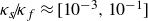 $\kappa _s \! / \! \kappa _f \approx [ 10^{-3}, 10^{-1} ]$
(see again table 1). Such values are not only clearly between the typically studied cases of
$\kappa _s \! / \! \kappa _f \approx [ 10^{-3}, 10^{-1} ]$
(see again table 1). Such values are not only clearly between the typically studied cases of
 $\kappa _s \! / \! \kappa _f \rightarrow 0$
and
$\kappa _s \! / \! \kappa _f \rightarrow 0$
and
 $\kappa _s \! / \! \kappa _f \rightarrow \infty$
, but also shifted towards the only more recently investigated Neumann case (Vieweg et al. Reference Vieweg, Scheel and Schumacher2021, Reference Vieweg, Scheel, Stepanov and Schumacher2022, Reference Vieweg, Klünker, Schumacher and Padberg-Gehle2024; Vieweg Reference Vieweg2024
a). Albeit we have covered corresponding values of
$\kappa _s \! / \! \kappa _f \rightarrow \infty$
, but also shifted towards the only more recently investigated Neumann case (Vieweg et al. Reference Vieweg, Scheel and Schumacher2021, Reference Vieweg, Scheel, Stepanov and Schumacher2022, Reference Vieweg, Klünker, Schumacher and Padberg-Gehle2024; Vieweg Reference Vieweg2024
a). Albeit we have covered corresponding values of
 $\kappa _s \! / \! \kappa _f$
, natural flows exhibit far greater
$\kappa _s \! / \! \kappa _f$
, natural flows exhibit far greater
 $Ra$
and potentially smaller
$Ra$
and potentially smaller
 $Pr$
as well as additional mechanisms like rotation (Schumacher & Sreenivasan Reference Schumacher and Sreenivasan2020; Vieweg et al. Reference Vieweg, Scheel, Stepanov and Schumacher2022). This present study can be seen as an important, yet early step towards understanding these more demanding and sophisticated geophysical and astrophysical systems. Our recent work (Vieweg et al. Reference Vieweg, Käufer, Cierpka and Schumacher2025) already started investigating asymmetric top and bottom plates and thermal boundary conditions as present in scientific engineering applications. Together with additional rotation around the vertical axis (Vieweg et al. Reference Vieweg, Scheel, Stepanov and Schumacher2022), this may represent an interesting potential path for future extensions relevant to core–core–mantle or core–ocean–ice configurations found on Earth or icy moons, respectively. Given this last discussion, the present work can define a starting point for further investigations on non-ideal boundary condition effects only.
$Pr$
as well as additional mechanisms like rotation (Schumacher & Sreenivasan Reference Schumacher and Sreenivasan2020; Vieweg et al. Reference Vieweg, Scheel, Stepanov and Schumacher2022). This present study can be seen as an important, yet early step towards understanding these more demanding and sophisticated geophysical and astrophysical systems. Our recent work (Vieweg et al. Reference Vieweg, Käufer, Cierpka and Schumacher2025) already started investigating asymmetric top and bottom plates and thermal boundary conditions as present in scientific engineering applications. Together with additional rotation around the vertical axis (Vieweg et al. Reference Vieweg, Scheel, Stepanov and Schumacher2022), this may represent an interesting potential path for future extensions relevant to core–core–mantle or core–ocean–ice configurations found on Earth or icy moons, respectively. Given this last discussion, the present work can define a starting point for further investigations on non-ideal boundary condition effects only.
Acknowledgements
P.P.V. gratefully acknowledges the support of Pembroke College, Cambridge, through a postdoctoral research associateship.
Funding
P.P.V. is funded by the Deutsche Forschungsgemeinschaft (DFG, German Research Foundation) within Walter Benjamin Programme 532721742. M.E. is funded by the Carl Zeiss Foundation with project number P2022-08-006. The authors gratefully acknowledge the Gauss Centre for Supercomuting e.V. (www.gauss-centre.eu) for funding this work by providing computing resources through the John von Neumann Institute for Computing (NIC) on the GCS supercomputer JUWELS at Jülich Supercomputing Center (JSC) within project nonbou. They further acknowledge the computing centre of the Technische Universität Ilmenau for providing access to, as well as computing and storage resources on its compute cluster MaPaCC24.
Declaration of interests
The authors report no conflict of interest.
Author contributions
P.P.V. and J.S. designed the study. M.E. performed the numerical simulations and processed the generated data. All authors contributed equally in discussing the data and writing the paper.
Appendix A. Linear stability analysis for the coupled system
A.1. Key idea of the linear stability analysis
The aim of the linear stability analysis is to find the point of the onset of convection with the fluid being initially at rest. The system is considered stable if perturbations, induced as infinitesimally small fluctuations in the form of planar waves, decay. Vice versa, it is unstable if such perturbations grow over time. The analysis is termed linear since one linearises the governing equations with respect to the (infinitesimally small) perturbations.
As it will turn out, the point of the onset of convection is determined by the critical Rayleigh number
 $Ra_{c}$
and is caused by the normal mode of the critical wavenumber
$Ra_{c}$
and is caused by the normal mode of the critical wavenumber
 $k_{c}$
. In order to transition from a linearly stable to a linearly unstable state, the system must pass the so-called marginal state – which is exactly the one defining these critical numbers (Chandrasekhar Reference Chandrasekhar1981).
$k_{c}$
. In order to transition from a linearly stable to a linearly unstable state, the system must pass the so-called marginal state – which is exactly the one defining these critical numbers (Chandrasekhar Reference Chandrasekhar1981).
In the following, the linear stability analysis for the CHT case will be performed. This will yield not only the neutral stability curves for different thermal conductivity ratios
 $\lambda _s \! / \! \lambda _f$
, the former of which represent the marginal states via
$\lambda _s \! / \! \lambda _f$
, the former of which represent the marginal states via
 $Ra ( k )$
, but also the critical Rayleigh numbers
$Ra ( k )$
, but also the critical Rayleigh numbers
 $Ra_{c}$
and wavenumbers
$Ra_{c}$
and wavenumbers
 $k_{c}$
as given by their global minimum.
$k_{c}$
as given by their global minimum.
A.2. Governing equations and boundary conditions
We consider the same set-up as shown in figure 1(b). As long as
 $Ra\!\lt \!Ra_{c}$
, we are in a non-convective regime and the fluid is at rest. As mentioned in § 2.2 and laid out in more detail in Vieweg et al. (Reference Vieweg, Käufer, Cierpka and Schumacher2025), in both the solids and the fluid the temperature profile will be linear. For further analysis it will be beneficial to use the temperature deviation
$Ra\!\lt \!Ra_{c}$
, we are in a non-convective regime and the fluid is at rest. As mentioned in § 2.2 and laid out in more detail in Vieweg et al. (Reference Vieweg, Käufer, Cierpka and Schumacher2025), in both the solids and the fluid the temperature profile will be linear. For further analysis it will be beneficial to use the temperature deviation
 $\varTheta (\boldsymbol{x}, t)$
. It is the deviation of the actual temperature profile from the linear one (which is present in a non-convective case) for both the solids and the fluid
$\varTheta (\boldsymbol{x}, t)$
. It is the deviation of the actual temperature profile from the linear one (which is present in a non-convective case) for both the solids and the fluid
 \begin{align} \varTheta _{\Phi }(\boldsymbol{x},t) = T_{\Phi }(\boldsymbol{x},t) - T_{lin,{\Phi }}(z), \quad \textrm {with} \quad \Phi =\{f,sb,st\}. \end{align}
For this analysis, we use the governing equations (2.1)–(2.4) based on a different non-dimensionalisation. Instead of the free-fall-inertia-balance (favourable for large
 $Re$
), we consider a scaling based on the viscous diffusion time scale
$Re$
), we consider a scaling based on the viscous diffusion time scale
 $\tau _{\nu }=H^2 / \nu$
leading to
$\tau _{\nu }=H^2 / \nu$
leading to
 \begin{align}&\qquad\qquad\qquad \tilde {\boldsymbol{\nabla} } \boldsymbol{\cdot} \tilde {\boldsymbol{u}} = 0, \end{align}
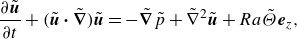 \begin{align}& \frac {\partial \tilde {\boldsymbol{u}}}{\partial t} + ( \tilde {\boldsymbol{u}} \boldsymbol{\cdot} \tilde {\boldsymbol{\nabla} } ) \tilde {\boldsymbol{u}} = - \tilde {\boldsymbol{\nabla} } \tilde {p} + \tilde {\nabla }^2 \tilde {\boldsymbol{u}} + Ra \tilde {\varTheta } \boldsymbol{e}_{z}, \end{align}
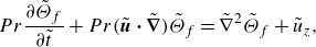 \begin{align}&\, {Pr} \frac {\partial \tilde {\varTheta }_{f}}{\partial \tilde {t}} + {Pr} (\tilde {\boldsymbol{u}} \boldsymbol{\cdot} \tilde {\boldsymbol{\nabla} } ) \tilde {\varTheta }_{f} = \tilde {\nabla }^2 \tilde {\varTheta }_{f} + \tilde {u}_z, \end{align}
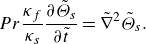 \begin{align}&\qquad\qquad {Pr} \frac {\kappa _f}{\kappa _s} \frac {\partial \tilde {\varTheta }_{s}}{\partial \tilde {t}} = \tilde {\nabla }^2 \tilde {\varTheta }_{s}. \end{align}
Equations (A2)–(A5) are completed by corresponding boundary conditions. In our set-up, mechanical no-slip boundary conditions are applied at both interfaces. Due to the present symmetry in our domain, we place the origin of the
 $z$
-coordinate at the midplane of the fluid layer. Together with the continuity equation (A2), this results in
$z$
-coordinate at the midplane of the fluid layer. Together with the continuity equation (A2), this results in
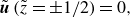 \begin{align} \tilde {\boldsymbol{u}} \left (\tilde {z} =\pm 1/2 \right ) &= 0 , \end{align}
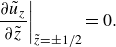 \begin{align} \left . \frac {\partial \tilde {u}_z}{\partial \tilde {z}}\right |_{\tilde {z} = \pm 1/2} & = 0. \end{align}
As the subdomains are coupled at the solid–fluid interfaces, both the temperatures and heat fluxes must match there which leads to
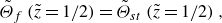 \begin{align}&\,\,\,\, \tilde {\varTheta }_{f} \left ( \tilde {z}=1/2 \right ) = \tilde {\varTheta }_{st} \left ( \tilde {z}=1/2 \right ), \end{align}
 \begin{align}& \tilde {\varTheta }_{f} \left ( \tilde {z}=-1/2 \right ) = \tilde {\varTheta }_{sb} \left ( \tilde {z}=-1/2 \right ), \end{align}
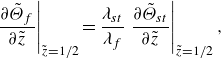 \begin{align}&\,\,\, \left .\frac {\partial \tilde {\varTheta }_{f}}{\partial \tilde {z}} \right |_{\tilde {z}=1/2} = \frac {\lambda _{st}}{\lambda _{f}} \left .\frac {\partial \tilde {\varTheta }_{st}}{\partial \tilde {z}} \right |_{\tilde {z}=1/2}, \end{align}
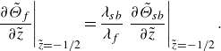 \begin{align} \left . \frac {\partial \tilde {\varTheta }_{f}}{\partial \tilde {z}} \right |_{\tilde {z}=-1/2} = \frac {\lambda _{sb}}{\lambda _{f}} \left . \frac {\partial \tilde {\varTheta }_{sb}}{\partial \tilde {z}} \right |_{\tilde {z}=-1/2}. \end{align}
We shall omit the tildes in the following for better readability.
A.3. Perturbation equations
Next, we apply infinitesimally small perturbations to the system by using a linear combination of basic perturbations. This forms a full set and allows us to extract the one at which instability first occurs. All variables will be subject to the perturbation
 $\phi '$
with
$\phi '$
with
 $\varepsilon \ll 1$
as a perturbation parameter, such that the base state
$\varepsilon \ll 1$
as a perturbation parameter, such that the base state
 $\bar {\phi }$
is disturbed via
$\bar {\phi }$
is disturbed via
 \begin{align} \phi = \bar {\phi } + \varepsilon \phi ' \quad \text{for} \quad \phi = \{\boldsymbol{u},p,\varTheta \}. \end{align}
Applying the curl to (A3) twice allows us to drop the pressure term. At this point, the infinitesimally small perturbations are applied to all variables. Keeping in mind that the fluid is at rest and the temperature deviation is absent for the base state, implying
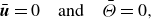 \begin{align} \bar {\boldsymbol{u}}=0\quad\textrm{and} \quad \bar {\varTheta }=0 , \end{align}
as well as dividing by
 $\varepsilon \neq 0$
and dropping all terms of
$\varepsilon \neq 0$
and dropping all terms of
 $\textit {O} ( \varepsilon ^2 )$
since
$\textit {O} ( \varepsilon ^2 )$
since
 $\varepsilon \ll 1$
(i.e.
$\varepsilon \ll 1$
(i.e.
 $\varepsilon ^2 \lll 1$
) yields the linearised equations
$\varepsilon ^2 \lll 1$
) yields the linearised equations
 \begin{align}&\qquad\qquad\qquad\quad \boldsymbol{\nabla} \boldsymbol{\cdot} \boldsymbol{u}' = 0, \end{align}
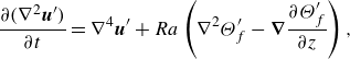 \begin{align}& \frac {\partial (\nabla ^2\boldsymbol{u}')}{\partial t} = \nabla ^4 \boldsymbol{u}' + Ra \left ( \nabla ^2 \varTheta _{f}' - \boldsymbol{\nabla} \frac {\partial \varTheta _{f}'}{\partial z} \right ), \end{align}
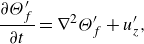 \begin{align}&\qquad\qquad\quad \frac {\partial \varTheta _{f}'}{\partial t} = \nabla ^2 \varTheta _{f}' + u_z', \end{align}
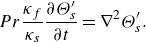 \begin{align}&\qquad\qquad\quad {Pr} \frac {\kappa _f}{\kappa _s} \frac {\partial \varTheta _{s}'}{\partial t} = \nabla ^2 \varTheta _{s}'. \end{align}
In a next step, a normal mode ansatz is applied: we assume an infinitely extended domain in the horizontal directions (in line with our laterally periodic boundary conditions) and use the linear equations (A14)–(A17) to superpose plane waves or normal modes which form a complete set of basis functions. These key features allow for linear superposition in the first place and later for an extraction of the wave at which instability occurs first. Such plane waves are given by
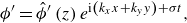 \begin{align} \phi ' = \hat {\phi }' \left ( z \right ) e^{ \mathrm{i} \left ( k_x x + k_y y \right ) + \sigma t }, \end{align}
where
 $k_{x,y}$
are the wavenumbers in
$k_{x,y}$
are the wavenumbers in
 $x$
and
$x$
and
 $y$
directions, defining the horizontal wavenumber
$y$
directions, defining the horizontal wavenumber
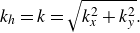 \begin{align} k_{h}=k=\sqrt {k_x^2+k_y^2}. \end{align}
Here
 $\sigma \in \mathbb{C}$
is the growth rate. Each perturbation
$\sigma \in \mathbb{C}$
is the growth rate. Each perturbation
 $\phi '$
in (A14)–(A17) is expressed via (A18) in terms of normal modes. Exemplary for the continuity equation, this results in
$\phi '$
in (A14)–(A17) is expressed via (A18) in terms of normal modes. Exemplary for the continuity equation, this results in
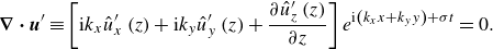 \begin{align} \boldsymbol{\nabla} \boldsymbol{\cdot} \boldsymbol{u}' \equiv &\left [ \mathrm{i} k_x \hat {u}_x'\left ( z \right ) +\mathrm{i}k_y \hat {u}_y'\left ( z \right ) + \frac {\partial \hat {u}_z' \left ( z \right ) }{\partial z} \right ] e^{\mathrm{i}\left ( k_x x + k_y y \right ) + \sigma t} = 0. \end{align}
For abbreviation, we define
 \begin{align} U:=\hat {u}_x' \left ( z \right ),\quad V:=\hat {u}_y' \left ( z \right ), \quad W:=\hat {u}_z' \left ( z \right ), \quad \hat {\varTheta }' \left ( z \right ) = \varTheta ,\quad D\phi :=\frac {\partial \left ( \phi \right )}{\partial z}, \end{align}
such that (A20) translates to simply
 \begin{align} \mathrm{i}k_x U +\mathrm{i}k_y V + D W = 0. \end{align}
Applying this in a similar fashion to (A15) in
 $z$
and (A16)–(A17), we obtain
$z$
and (A16)–(A17), we obtain
 \begin{align}& \sigma \big ( D^2-k^2 \big ) W = \big ( D^2 -k^2 \big )^2 W - Ra k^2 \varTheta _{f}, \end{align}
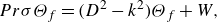 \begin{align}&\qquad\quad {Pr} \sigma \varTheta _{f} = \big ( D^2 -k^2 \big ) \varTheta _{f} + W, \end{align}
 \begin{align}&\qquad\quad\,\,\, {Pr} \frac {\kappa _f}{\kappa _s} \sigma \varTheta _{s} = \big ( D^2 - k^2 \big ) \varTheta _{s}. \end{align}
On the other hand, the boundary conditions (A6)–(A11) translate to
 \begin{align}&\qquad\quad\,\,\, W\left ( z=\pm 1/2 \right ) = 0, \end{align}
 \begin{align}&\qquad\qquad DW |_{ z=\pm 1/2 } = 0, \end{align}
 \begin{align}&\,\,\, \varTheta _{f} \left ( z= 1/2 \right ) = \varTheta _{st} \left ( z=1/2 \right ), \end{align}
 \begin{align}& \varTheta _{f} \left ( z= -1/2 \right ) = \varTheta _{sb} \left ( z= -1/2 \right ), \end{align}
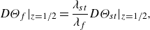 \begin{align}&\quad D \varTheta _{f} |_{z=1/2} = \frac {\lambda _{st}}{\lambda _{f}} D \varTheta _{st} |_{z=1/2}, \end{align}
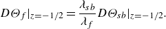 \begin{align}&\,\, D \varTheta _{f} |_{z=-1/2} = \frac {\lambda _{sb}}{\lambda _{f}} D \varTheta _{sb} |_{z=-1/2}. \end{align}
A.4. Marginally stable state
The marginally stable state is the one we are looking for, defining neutral stability. Depending on the imaginary part of the growth rate, the system may be in overstability, if for at least one wavenumber
 $\textrm {Im} ( \sigma ) \neq 0$
. Otherwise, if all wavenumbers result in an imaginary part of
$\textrm {Im} ( \sigma ) \neq 0$
. Otherwise, if all wavenumbers result in an imaginary part of
 $0$
, the principle of exchange of stabilities is valid.
$0$
, the principle of exchange of stabilities is valid.
Chandrasekhar (Reference Chandrasekhar1981) has shown that the latter applies for the Rayleigh–Bénard convection set-up. Moreover, Hurle has adapted this to the CHT case, allowing for the application of this principle (Hurle et al. Reference Hurle, Jakeman and Pike1967). Thus, we can set
 \begin{align} \textrm {Re} \left ( \sigma \right ) \stackrel {!}{=} 0 \land \textrm {Im} \left ( \sigma \right ) \stackrel {!}{=} 0 \Rightarrow \sigma \equiv 0. \end{align}
Applying this to (A23)–(A25) gives us our modelling equations. We can rewrite (A24)
 \begin{align} \underbrace {{Pr} \sigma \varTheta _{f}}_{\sigma =0} = \big ( D^2 -k^2 \big ) \varTheta _{f} + W \Leftrightarrow \varTheta _{f} = - \frac {W}{D^2-k^2} \, \, \textrm {or} \, \, W = - \big ( D^2-k^2 \big ) \varTheta _{f} , \end{align}
and insert it into (A23), yielding either an ordinary differential equation for
 $W$
,
$W$
,
 \begin{align} \big ( \big ( D^2-k^2 \big )^3 + Ra k^2\big ) W = 0 \end{align}
or, alternatively, for
 $\varTheta _{f}$
 \begin{align} \big ( D^2 -k^2 \big ) \big ( \big ( D^2 -k^2 \big )^3 + Ra k^2 \big ) \varTheta _{f} = 0 . \end{align}
For the solids, in turn,
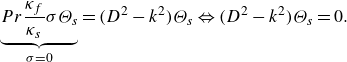 \begin{align} \underbrace {{Pr} \frac {\kappa _f}{\kappa _s} \sigma \varTheta _{s}}_{\sigma =0} &= \big ( D^2 - k^2 \big ) \varTheta _{s} \Leftrightarrow \big ( D^2 -k^2 \big ) \varTheta _{s} = 0. \end{align}
An interesting aspect of (A34)–(A36) is that the dependence on the Prandtl number
 $Pr$
cancels out (because we assumed
$Pr$
cancels out (because we assumed
 $\sigma \equiv 0$
). Furthermore, all three equations are linear ordinary partial differential equations, making them comparatively easy to solve.
$\sigma \equiv 0$
). Furthermore, all three equations are linear ordinary partial differential equations, making them comparatively easy to solve.
A.5. Solution of the modelling equations
Dealing with linear ordinary differential equations, an exponential ansatz of the form
 \begin{align} \phi \left ( z \right ) = e^{qz}, \quad \phi = \{ W, \varTheta _{f}, \varTheta _{sb}, \varTheta _{st} \} \end{align}
with the free parameter
 $q$
is usually promising. Starting with the simplest of the three equations for the temperature deviation, that in the solids
$q$
is usually promising. Starting with the simplest of the three equations for the temperature deviation, that in the solids
 $\varTheta _{sb,st}$
(A36), we get
$\varTheta _{sb,st}$
(A36), we get
 \begin{align} \big ( D^2 -k^2 \big ) \varTheta _{s} = 0 \Rightarrow \varTheta _{s} \left ( z \right ) = c_1 e^{-kz} + c_2 e^{kz}. \end{align}
At the very top and bottom of the plates, respectively, temperature deviations must be
 $0$
as the temperature is set by virtue of the (external) thermal boundary conditions. Thus, we apply
$0$
as the temperature is set by virtue of the (external) thermal boundary conditions. Thus, we apply
 \begin{align} &\,\,\,\varTheta _{st} \left ( z=1/2+\Gamma _{st} \right ) \stackrel {\small ({\textrm{A38}})}{\Longrightarrow }\quad \varTheta _{st} \left ( z \right ) = c_1 \big ( e^{-kz} - e^{kz} e^{-k(1+2\Gamma _{st})} \big ), \end{align}
 \begin{align} &\varTheta _{sb} \left ( z=- \left (1/2+\Gamma _{sb} \right ) \right ) \stackrel {\small ({\textrm{A38}})}{\Longrightarrow } \varTheta _{sb} \left ( z \right ) = c_2 \big ( e^{kz} - e^{-kz} e^{-k(1+2\Gamma _{sb})} \big ). \end{align}
Solving (A34) and (A35) with this the exponential ansatz leads to
 \begin{align} &\qquad\,\,\big ( \big ( q^2 - k^2 \big )^3 + Ra \, k^2 \big ) W = 0 , \end{align}
 \begin{align}& \big ( q^2 -k^2 \big ) \big ( \big ( q^2 -k^2 \big )^3 + Ra\, k^2 \big ) \varTheta _{f} = 0 \end{align}
whereas we obtain
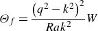 \begin{align} \varTheta _{f} = \frac {\left ( q^2 -k^2 \right )^2}{Ra k^2} W \end{align}
using (A23) when setting
 $\sigma =0$
and using the same exponential ansatz. We obtain the solutions
$\sigma =0$
and using the same exponential ansatz. We obtain the solutions
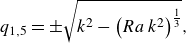 \begin{align}&\qquad\quad q_{1,5} = \pm \sqrt {k^2 - \left ( Ra \, k^2 \right )^{\frac {1}{3}}}, \end{align}
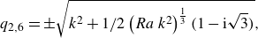 \begin{align}& q_{2,6} = \pm \sqrt {k^2 + 1/2 \left ( Ra \, k^2 \right )^{\frac {1}{3}}\big ( 1-\mathrm{i}\sqrt {3} \big )}, \end{align}
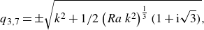 \begin{align}& q_{3,7} = \pm \sqrt {k^2 + 1/2 \left ( Ra \, k^2 \right )^{\frac {1}{3}}\big ( 1+\mathrm{i}\sqrt {3} \big )}, \\[-12pt] \nonumber \end{align}
 \begin{align}&\qquad\qquad\qquad q_{4,8} = \pm k, \end{align}
where
 $q_{4,8}$
applies to (A42) only whereas the other solutions are valid for both (A41) and (A42).
$q_{4,8}$
applies to (A42) only whereas the other solutions are valid for both (A41) and (A42).
Looking at the
 $ ( q^2 - k^2 )$
-term in (A41) and (A42), one can observe symmetry. Therefore, the solution may be written as a combination of
$ ( q^2 - k^2 )$
-term in (A41) and (A42), one can observe symmetry. Therefore, the solution may be written as a combination of
 $\sinh$
and
$\sinh$
and
 $\cosh$
with orthogonal basis functions, splitting the overall solution into the even and odd solutions
$\cosh$
with orthogonal basis functions, splitting the overall solution into the even and odd solutions
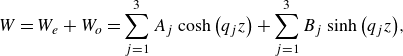 \begin{align}&\qquad\qquad\quad W = W_e + W_o = \sum _{j=1}^3 A_j \cosh {\left ( q_j z \right ) } + \sum _{j=1}^3 B_j \sinh {\left ( q_j z \right )}, \end{align}
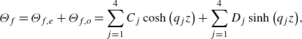 \begin{align}&\qquad\qquad \varTheta _{f} = \varTheta _{f,e} + \varTheta _{f,o} = \sum _{j=1}^4 C_j \cosh {\left ( q_j z \right ) } + \sum _{j=1}^4 D_j \sinh {\left ( q_j z \right )}, \end{align}
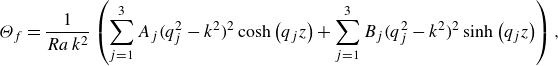 \begin{align}& \varTheta _{f} = \frac {1}{Ra \, k^2} \left ( \sum _{j=1}^3 A_j \big ( q_j^2-k^2 \big )^2 \cosh {\left ( q_j z \right ) } + \sum _{j=1}^3 B_j \big ( q_j^2-k^2 \big )^2 \sinh {\left ( q_j z \right )} \right ), \end{align}
A.6. Applying the boundary conditions
Now we apply the boundary conditions (A26)–(A31) to solve (A48) and (A49) while using these conditions for the solids (A39) and (A40). For each condition, (A48) and (A49) are split into even and odd modes and solved separately. Regarding identical bottom and top plates, we can further set
 \begin{align} \lambda _{st} = \lambda _{sb} = \lambda _{\mathrm{s}}, \end{align}
 \begin{align} \Gamma _{st} = \Gamma _{sb} = {\Gamma _s}. \end{align}
Note that this makes the boundary conditions for the solid bottom domain obsolete as the solution coincides with that of the solid top domain by virtue of symmetry. For (A26), one obtains
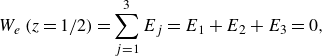 \begin{align} W_e \left (z=1/2 \right ) &= \sum _{j=1}^3 E_j = E_1 + E_2 + E_3 = 0, \end{align}
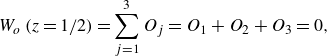 \begin{align} W_o \left (z=1/2 \right ) &= \sum _{j=1}^3 O_j = O_1 + O_2 + O_3 = 0, \end{align}
with the new constants
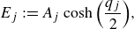 \begin{align} E_j&:=A_j \cosh {\left ( \frac {q_j}{2} \right )}, \end{align}
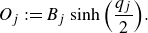 \begin{align} O_j&:=B_j \sinh {\left ( \frac {q_j}{2} \right )}. \end{align}
Applying (A27) yields
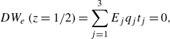 \begin{align} DW_e \left ( z=1/2 \right ) &= \sum _{j=1}^3 E_j q_j t_j = 0, \end{align}
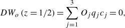 \begin{align} DW_o \left ( z=1/2 \right ) &= \sum _{j=1}^3 O_j q_j c_j = 0, \end{align}
with
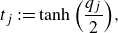 \begin{align} t_j := \tanh {\left ( \frac {q_j}{2} \right )}, \end{align}
 \begin{align} c_j := \coth {\left ( \frac {q_j}{2} \right )} . \end{align}
For (A28) one gets
 \begin{align} -E_0 {\frac {\lambda _f}{\lambda _s}} \tanh {\left ( k {{\Gamma _s}} \right )} + \frac {1}{Ra \, k^2} \sum _{j=1}^3 E_j \big ( q_j^2-k^2 \big )^2 &= 0, \end{align}
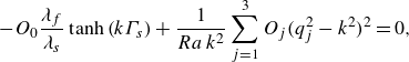 \begin{align} -O_0 {\frac {\lambda _f}{\lambda _s}} \tanh {\left ( k {{\Gamma _s}} \right )} + \frac {1}{Ra \, k^2} \sum _{j=1}^3 O_j \big ( q_j^2-k^2 \big )^2 &= 0, \end{align}
where the new constant is
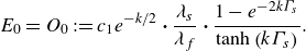 \begin{align} E_0 = O_0 := c_1 e^{-k/2} \boldsymbol{\cdot} {\frac {\lambda _s}{\lambda _f}} \boldsymbol{\cdot} \frac {1-e^{-2k{{\Gamma _s}}}}{\tanh {\left ( k {{\Gamma _s}} \right )}} . \end{align}
Finally, for (A30) one obtains
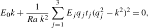 \begin{align} E_0k + \frac {1}{Ra \, k^2} \sum _{j=1}^3 E_j q_j t_j \big ( q_j^2-k^2 \big )^2 &= 0, \end{align}
 \begin{align} O_0k + \frac {1}{Ra \, k^2} \sum _{j=1}^3 O_j q_j c_j \big( q_j^2-k^2 \big )^2 &= 0. \end{align}
As a result, we are left with two systems of equations: One for the even modes and one for the odd modes. Together with the parameter
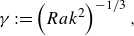 \begin{align} \gamma := \left ( Ra k^2 \right )^{-1/3} , \end{align}
(A64) and (A65) can be written as
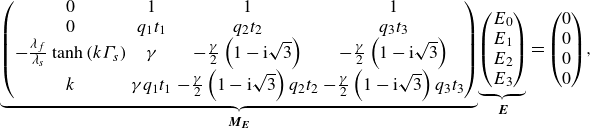 \begin{align}& \underbrace { \begin{pmatrix} 0 & 1 & 1 & 1 \\ 0 & q_1t_1 & q_2t_2 & q_3t_3 \\ - \frac {\lambda _f}{\lambda _s} \tanh {\left (k{\Gamma _s} \right )} & \gamma & -\frac {\gamma }{2} \left ( 1-\mathrm{i} \sqrt {3} \right ) & -\frac {\gamma }{2} \left ( 1-\mathrm{i} \sqrt {3} \right ) \\ k & \gamma q_1t_1 & -\frac {\gamma }{2} \left ( 1-\mathrm{i} \sqrt {3} \right ) q_2t_2 & -\frac {\gamma }{2} \left ( 1-\mathrm{i} \sqrt {3} \right ) q_3t_3 \end{pmatrix} }_{\boldsymbol{M_E}} \!\underbrace { \begin{pmatrix} E_0 \\ E_1 \\ E_2 \\ E_3 \end{pmatrix} }_{\boldsymbol{E}} = \begin{pmatrix} 0 \\ 0 \\ 0 \\ 0 \end{pmatrix}\!, \end{align}
 \begin{align} &\underbrace { \begin{pmatrix} 0 & 1 & 1 & 1 \\ 0 & q_1c_1 & q_2c_2 & q_3c_3 \\ - \frac {\lambda _f}{\lambda _s} \tanh {\left (k{\Gamma _s} \right )} & \gamma & -\frac {\gamma }{2} \left ( 1-\mathrm{i} \sqrt {3} \right ) & -\frac {\gamma }{2} \left ( 1-\mathrm{i} \sqrt {3} \right ) \\ k & \gamma q_1c_1 & -\frac {\gamma }{2} \left ( 1-\mathrm{i} \sqrt {3} \right ) q_2c_2 & -\frac {\gamma }{2} \left ( 1-\mathrm{i} \sqrt {3} \right ) q_3c_3 \end{pmatrix} }_{\boldsymbol{M_O}} \!\underbrace { \begin{pmatrix} O_0 \\ O_1 \\ O_2 \\ O_3 \end{pmatrix} }_{\boldsymbol{O}} = \begin{pmatrix} 0 \\ 0 \\ 0 \\ 0 \end{pmatrix}\!. \end{align}
In other words, both the even and odd solutions represent a system of four equations which must be solved at once. Note that the involved
 $q_j$
,
$q_j$
,
 $t_j$
,
$t_j$
,
 $c_j$
and
$c_j$
and
 $\gamma$
are defined in (A44)–(A46), (A59), (A60) and (A66), respectively. The trivial solutions, i.e. all constants
$\gamma$
are defined in (A44)–(A46), (A59), (A60) and (A66), respectively. The trivial solutions, i.e. all constants
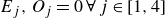 $E_j,O_j=0 \, \forall \, j \in [ 1,4 ]$
, are obvious. To find the non-trivial solution, the determinants of the given coefficient matrices
$E_j,O_j=0 \, \forall \, j \in [ 1,4 ]$
, are obvious. To find the non-trivial solution, the determinants of the given coefficient matrices
 $\boldsymbol{M_E}, \boldsymbol{M_O}$
must contract to zero.
$\boldsymbol{M_E}, \boldsymbol{M_O}$
must contract to zero.
In this solution, there are four free variables left:
 $\Gamma _s$
,
$\Gamma _s$
,
 $\lambda _f \! / \! \lambda _s$
,
$\lambda _f \! / \! \lambda _s$
,
 $k$
and
$k$
and
 $Ra$
. This allows us to fix
$Ra$
. This allows us to fix
 $\Gamma _s$
and
$\Gamma _s$
and
 $\lambda _f \! / \! \lambda _s$
to compute the neutral stability curves
$\lambda _f \! / \! \lambda _s$
to compute the neutral stability curves
 $Ra ( k )$
for the even and odd solutions.
$Ra ( k )$
for the even and odd solutions.
We find that odd solutions are generally more stable than even solutions. In other words, the neutral stability curves from even solution are below those from odd solutions. Hence, we restrict our analysis in the main text, see (3.1), to the solution of (A67).
Appendix B. Convergence of thermal boundary conditions at extreme ratios of thermal diffusivities
$\boldsymbol{\kappa} _{\boldsymbol{s}} \! \boldsymbol{/} \! \boldsymbol{\kappa} _{\boldsymbol{f}}$

In order to validate our CHT set-up – which adds two identical fluid-confining solid plates at the top and bottom of the classically studied fluid layer – we conduct two simulations using extreme
 $\kappa _s \! / \! \kappa _f = \left \{ 10^{-6}, 10^{6} \right \}$
. These parameters are supposed to resemble the idealised Neumann and Dirichlet case,
$\kappa _s \! / \! \kappa _f = \left \{ 10^{-6}, 10^{6} \right \}$
. These parameters are supposed to resemble the idealised Neumann and Dirichlet case,
 $\kappa _s \! / \! \kappa _f \rightarrow 0$
and
$\kappa _s \! / \! \kappa _f \rightarrow 0$
and
 $\kappa _s \! / \! \kappa _f \rightarrow \infty$
, respectively.
$\kappa _s \! / \! \kappa _f \rightarrow \infty$
, respectively.
For understanding these limits and their consequences, it is helpful to think of our CHT set-up as a thermal circuit with its different involved thermal resistances or conductances (representing, e.g. the different subdomains) (Incopera et al. Reference Incropera, DeWitt, Bergman and Lavine2007; Vieweg et al. Reference Vieweg, Käufer, Cierpka and Schumacher2025). If one pathway of heat transfer offers a significantly smaller thermal resistance
 $R_{th}$
– or, as
$R_{th}$
– or, as
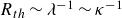 $R_{th} \sim \lambda ^{-1} \sim \kappa ^{-1}$
, larger thermal conductivity or diffusivity – it represents a shortcut and will be favoured over other pathways.
$R_{th} \sim \lambda ^{-1} \sim \kappa ^{-1}$
, larger thermal conductivity or diffusivity – it represents a shortcut and will be favoured over other pathways.
In case of
 $\kappa _s \! / \! \kappa _f \rightarrow 0$
or
$\kappa _s \! / \! \kappa _f \rightarrow 0$
or
 $\kappa _{\textrm {s}} \ll \kappa _{\textrm {f}}$
, the thermal resistance of the solid plates is enormous. However, as our domain is horizontally periodic, heat transfer through these plates is unavoidable and the ‘easiest’ way through the plate is by passing it vertically. This means for the present set-up that heat transfer from
$\kappa _{\textrm {s}} \ll \kappa _{\textrm {f}}$
, the thermal resistance of the solid plates is enormous. However, as our domain is horizontally periodic, heat transfer through these plates is unavoidable and the ‘easiest’ way through the plate is by passing it vertically. This means for the present set-up that heat transfer from
 $T_h$
to
$T_h$
to
 $T_c$
tends to avoid ‘expensive’ horizontal transfer within the solid plates and results in a uniform heat flux at the solid–fluid interfaces. Thus, the classical Neumann case is resembled.
$T_c$
tends to avoid ‘expensive’ horizontal transfer within the solid plates and results in a uniform heat flux at the solid–fluid interfaces. Thus, the classical Neumann case is resembled.
In the opposite case of
 $\kappa _s \! / \! \kappa _f \rightarrow \infty$
or
$\kappa _s \! / \! \kappa _f \rightarrow \infty$
or
 $\kappa _{\textrm {s}} \gg \kappa _{\textrm {f}}$
, the thermal resistance of the solid plates is tiny whereas that of the fluid layer is huge. Heat transfer starting from
$\kappa _{\textrm {s}} \gg \kappa _{\textrm {f}}$
, the thermal resistance of the solid plates is tiny whereas that of the fluid layer is huge. Heat transfer starting from
 $T_h$
or towards
$T_h$
or towards
 $T_c$
will go all possible ways within the solid plates before eventually interacting with the resistive fluid layer. As a result, heat transfer within the solid plates is faster than through the fluid layer and the plates become isothermal, leading to the classical Dirichlet case.
$T_c$
will go all possible ways within the solid plates before eventually interacting with the resistive fluid layer. As a result, heat transfer within the solid plates is faster than through the fluid layer and the plates become isothermal, leading to the classical Dirichlet case.
Figure 12 compares our extreme CHT cases with classical, plateless scenarios. It is obvious that the more natural implementations of the Neumann and Dirichlet cases match their idealised counterparts very well. This first qualitative impression is further confirmed by
 $Nu$
,
$Nu$
,
 $Re$
and
$Re$
and
 $\varLambda _T$
as provided in table 4.
$\varLambda _T$
as provided in table 4.
The direct comparison of a plateless Neumann case and the plate-involving CHT case results in an artefact concerning the mean temperature difference across the fluid layer: in the Neumann case, the non-dimensionalisation is not based on the characteristic temperature
 $T_{char,D} = \Delta T$
(as in the Dirichlet and CHT cases) but rather on the applied vertical temperature gradient across the fluid layer
$T_{char,D} = \Delta T$
(as in the Dirichlet and CHT cases) but rather on the applied vertical temperature gradient across the fluid layer
 $T_{char,N} = - \partial T / \partial z$
. In other words, the characteristic temperature scale is different. As a result, the resulting mean temperature difference
$T_{char,N} = - \partial T / \partial z$
. In other words, the characteristic temperature scale is different. As a result, the resulting mean temperature difference
 $\Delta T_N \leqslant 1$
(Otero et al. Reference Otero, Wittenberg, Worthing and Doering2002). This leads to out-of-line scaling in the legend of figure 12 as well as
$\Delta T_N \leqslant 1$
(Otero et al. Reference Otero, Wittenberg, Worthing and Doering2002). This leads to out-of-line scaling in the legend of figure 12 as well as
 $\max ( \varDelta _h T )$
and
$\max ( \varDelta _h T )$
and
 $\mathrm{std} ( T )$
in table 4. However, this is more of a technical issue and can be circumvented by rescaling the solution fields based on
$\mathrm{std} ( T )$
in table 4. However, this is more of a technical issue and can be circumvented by rescaling the solution fields based on
 $\Delta T_N$
(Vieweg Reference Vieweg2023Reference Vieweg2024a), eventually realigning the values and proving the validity of our used set-up.
$\Delta T_N$
(Vieweg Reference Vieweg2023Reference Vieweg2024a), eventually realigning the values and proving the validity of our used set-up.
Pattern formation at extreme ratios of thermal diffusivities
 $\kappa _s \! / \! \kappa _f$
. For extreme values of
$\kappa _s \! / \! \kappa _f$
. For extreme values of
 $\kappa _s \! / \! \kappa _f$
, (b,c) the flow patterns of CHT simulations converge perfectly towards (a,d) those obtained from classical idealised thermal boundary conditions. Here
$\kappa _s \! / \! \kappa _f$
, (b,c) the flow patterns of CHT simulations converge perfectly towards (a,d) those obtained from classical idealised thermal boundary conditions. Here
 $Ra = 10^{4}$
and
$Ra = 10^{4}$
and
 ${\Gamma _s} = 15$
(if applicable). Note that the simulations from panels (a,d) do not comprise any solid plates, whereas those from panels (b,c) do.
${\Gamma _s} = 15$
(if applicable). Note that the simulations from panels (a,d) do not comprise any solid plates, whereas those from panels (b,c) do.
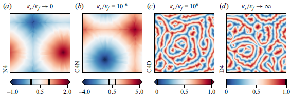


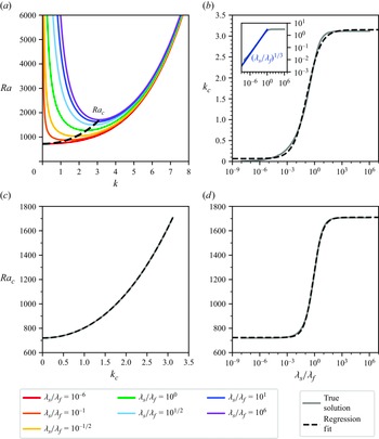


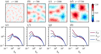


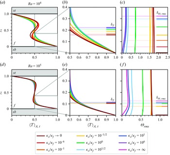


 Open access