1. Introduction
Numerical computer codes for ice-sheet flow emerge from two stages of effort, first the specification of a continuum model (i.e. partial differential equations) and second the numerical approximation of that model by a discrete computer code. The second stage is necessitated by the difficulty of identifying exact, analytical solutions to nonlinear partial differential equations for general initial and boundary conditions. It should be carefully verified because the results of numerical codes are, for problems as complex as ice flow, the primary means of extracting predictions from the continuum model.
Verification using exact solutions is the goal of the current paper. The ‘benchmarking’ of the second (numerical) stage is also the stated goal of the European Ice-Sheet Modelling Initiative (EISMINT) efforts (Reference Huybrechts and PayneHuybrechts and others, 1996; Reference PaynePayne and others, 2000; hereafter referred to as ‘EISMINT I’ and ‘EISMINT II’).
One would suppose from the EISMINT efforts that exact solutions to the simplest large class of ice-sheet models – isothermal and shallow – are in extremely short supply. In particular, only one two-dimensional (2-D) steady-state solution is referenced in EISMINT I and exact solutions are not mentioned in EISMINT II. We presume that lack of exact solutions is the motivation for benchmarking by intercomparison.
A moving-margin exact solution exists in the literature (Reference HalfarHalfar, 1981, Reference Halfar1983), however. Here we generalize the Reference HalfarHalfar (1983) radial similarity solution, and show it is the zero-accumulation case in a family of non-zero-accumulation similarity solutions. These solutions are all well suited for verifying numerical models. The Halfar solution appears in the literature as a Mars polar cap model by Nye (2000), and the two-dimensional (2-D) case of the solution (Reference HalfarHalfar, 1981) is discussed by Reference HindmarshHindmarsh (1990) and Reference Leysinger Vieli and GudmundssonLeysinger Vieli and Gudmundsson (2004). Unfortunately the Halfar solution does not appear in the standard textbooks (Reference HutterHutter, 1983; Reference PatersonPaterson, 1994; Reference FowlerFowler, 1997; Reference Van der VeenVan der Veen, 1999).
The supply of exact time-dependent solutions suitable for numerical verification is reasonably rich because we can also construct exact solutions with ‘compensatory accumulation’, a technique called the ‘method of manufactured solutions’ (Reference RoacheRoache, 1998) in computational fluid dynamics (CFD). Compensatory accumulations allow construction of an exact solution with oscillatory (in time) accumulation and an exact solution with basal sliding in an ice-stream-like sector, for instance. There exist enough exact solutions to verify all features of time-stepping shallow, isothermal numerical models.
In section 3 we propose a suite of tests based on the exact solutions derived in section 2. The proposed suite is used in section 4 to verify a standard explicit finite-difference method. This method has been selected for both ease of generalization to the thermocoupled case and also ease of exposition here. We expect that other numerical schemes will be verified by some selection of exact solutions and will show comparable or greater numerical quality (within the constraints discussed in section 5.1).
We use the term ‘verification’ for the comparison of very accurate solutions with the numerical approximations produced by a given code. The term ‘verification’ and a second term ‘validation’ are standard in the CFD literature. These terms are illustrated and informally defined in the following excerpt:
‘Two types of errors may be distinguished: modelling errors and numerical errors. Modelling errors arise from not solving the right equations. Numerical errors arise from not solving the equations right. The assessment of modelling errors is called validation, whereas the assessment of numerical errors is called verification... Validation makes sense only after verification, otherwise agreement between measured and computed results may well be fortuitous’ (Reference WesselingWesseling, 2001, p.560–561, emphasis in original).
Standards for verification in CFD are well established, as in the validation and verification guidelines of the American Institute of Aeronautics and Astronautics (AIAA, 1998) and the ‘best practice’ guidelines of the European Research Community On Flow, Turbulence And Combustion (ERCOFTAC, 2000). In summary, the standard for verification is the comparison of highly accurate solutions, usually exact solutions, to numerical results for a variety of cases sufficient to exercise all parts of the numerical scheme including boundary conditions; evidence of convergence to the continuum must be shown (AIAA, 1998). Note that verification is generally finished by the satisfaction of such a standard (until the code changes);validation is never completely finished for any non-trivial code and continuum model.
Advantages of verification by exact solutions vs intercomparison include: (i) In intercomparison certain features of the collected numerical results are chosen for comparison and reporting. Researchers with new goals may be interested in features not chosen. (ii) Convergence of numerical methods is hard to measure by intercomparison. (It was not attempted in EISMINT I.) ‘Convergence’ here refers to the decay to zero of the ice-sheet-wide maximum numerical error relative to highly accurate solutions as numerical parameters go to their continuum limit (Reference RoacheRoache, 1998) and not analysis of local truncation error (cf. Reference WaddingtonWaddington, 1981) by itself. (iii) Without an exact solution, there is no way to know the quality of a newly computed result which falls outside a reported intercomparison range. For a hypothetical example, suppose that in EISMINT I all codes had possessed diffusivity calculations of ‘type II’. In that case, a new code of ‘type I’ would produce thicknesses closer to the continuum values than any of the reported results, but would fall outside of the reported range. (iv) Exact solutions are more portable because they can be recreated by anyone who understands their derivation.
We do not view verification as an end in itself, of course. The goal is close approximation of ice-sheet behavior. In particular, it is desirable to compare the results of a variety of verified (to the extent possible) ice-sheet codes to field measurements and to compare the results of verified codes for distinct continuum models. A recent paper by Reference Leysinger Vieli and GudmundssonLeysinger Vieli and Gudmundsson (2004) performs exactly such a verified comparison of shallow and full-system (nonshallow) models in the 2-D isothermal, frozen-bed alpine glacier case. On the other hand, Reference MahaffyMahaffy’s (1976) classic work included validation relative to the contemporary state of Barnes Ice Cap, Canada.
In this paper, we consider exact solutions to the isothermal shallow case. We do not include ‘diagnostic’ temperature calculations for two reasons. First, high-quality (relative to EISMINT I and II grid choices) numerical results are known for temperature calculations in a fixed or changing geometry, though without full thermocoupling (Reference Calvo, Durany and VazquezCalvo and others, 1999, Reference Calvo, Durany and Vazquez2002a). Second, construction of exact solutions to the thermocoupled shallow ice-sheet model is also possible by manufacturing a solution. We will describe such solutions in a future paper. Such solutions allow verification of most of the features of the models addressed by EISMINT II. Finally, any reasonable thermocoupled code will have a mode in which the coupling can be turned off; this mode can be verified using the methods of the current paper.
2. Time-Dependent Exact Solutions
The notation of this paper matches, to the extent possible, that of EISMINT I. At position x, y and time t the ice-sheet thickness is H(x, y, t) meters. We suppose isostatic bed depression is described by a constant fraction f so that h =(1 – f)H is the surface elevation and –fH the bed elevation. Let M(x, y, t) (ma–1) be the rate of surface accumulation, negative for ablation. Throughout this paper, divergence and gradient are in horizontal variables.
Consider the isothermal shallow ice-sheet equation without basal sliding, an equation of mass continuity
where q f is the volume discharge due to internal deformation of the ice. Assuming the Reference GlenGlen (1955) constitutive relation as generalized by Reference Nye and NyeNye (1957), and using the shallow-ice approximation (Reference HutterHutter, 1983; Reference FowlerFowler, 1997), we have
where n is a fixed exponent in the range 1.8 < n < 4 (Reference Goldsby and KohlstedtGoldsby and Kohlstedt, 2001). EISMINT I parameterizes Г = 2A(pg)n=(n + 2), where A is a temperature-dependent flow-law parameter, p is the density of ice (assumed constant), and g is the acceleration due to gravity.
Either of two boundary conditions for ice sheets is supposed, along with Equations (1) and (2), to determine unique solutions. The natural condition is imposed by requiring H > 0 (Reference Hindmarsh, Greve, Ehrentraut and WangHindmarsh, 2001; Reference Calvo, Diaz, Durany, Schiavi and VazquezCalvo and others, 2002b). Such a boundary condition applies to grounded moving margins and to grounded steady margins in ablation zones where qf = 0. The Vialov–Nye condition H = 0, imposed at predetermined ice-free points, is a well-established first approximation to the complex boundary condition at a marine calving front. Typically ![]() at a Vialov–Nye margin. Both boundary conditions are of interest to modellers; section 5.1 addresses the difficulty of numerically approximating both types of margins.
at a Vialov–Nye margin. Both boundary conditions are of interest to modellers; section 5.1 addresses the difficulty of numerically approximating both types of margins.
The reader interested primarily in numerical verification may bypass the remainder of section 2, containing derivations of new exact solutions, and proceed to the exact-solution-based test suite in section 3 and an example verification using these tests in section 4. The results of the next three subsections can be (and have been) checked by substitution into the relevant differential equations.
2.1. A family of similarity solutions with non-zero accumulation
We now consider certain exact, time-dependent and radial solutions to Equations (1) and (2) with H ≥ 0, called similarity solutions. (See Reference BarenblattBarenblatt (1996) for examples of similarity solutions in other fields.) It turns out that such a solution exists if accumulation is proportional to thickness and is inversely proportional to time. In particular, as will be shown below, there is a similarity solution H = Hχ to the equation
where χ is an accumulation parameter explained below. Such solutions are useful for verifying a numerical code’s ability to respond to a time-dependent accumulation (source) term.
We seek a solution of the similarity form (ansatz)
where r is the radial distance r 2 = x 2 + y 2. (Regarding derivatives in radial directions, recall that Δ g = (dg/dr)ř and ∇ • (gř) = r— 1d(rg)/dr if g = g(r) and ř is the unit radial vector.) The constants α, 3 and the function φ are to be determined.
Following Reference HalfarHalfar (1983), one might try to start the derivation by supposing H(r, t) = aF2(t)G(brF(t)) for unknown constants α, b and unknown functions F, G. This leads to ordinary differential equations for F and G by separation but presupposes α = 23 which excludes a nonzero-accumulation solution. Similarly, the elegant derivation of Halfar’s solution in Nye (2000) starts from the assumption that the volume is constant;this is not true of the λ = 0 solutions here.
Instead, substitute H = H λ and h =(1 – f)Hλ into Equation (3). The course of the derivation that follows is best seen by noting that the conditions for eventual success are, most importantly,
Note that these equations completely determine α and 3 as functions of n and λ.
The role of the first of conditions (5) is to allow the elimination of t from the equation found by substituting the similarity form. The result is an ordinary differential equation
where (•)0 denotes d/ds. Equation (6) can be integrated once using the second of conditions (5) to write (α + λ)sφ + 3s2 φ’ = 3(s2φ)’; the constant of integration is seen to be zero because φ(0) and φ’(0) are finite. If φ’ < 0, i.e. if flow is in the positive radial direction, then
This equation is separable. Note φ (s) < 0 for some s > 0 implies 3 > 0.
For the next integration, suppose 3 > 0 and suppose that at time t 0 > 0 the dome thickness at r = 0 is H0. Integrating Equation (7) yields
Let R
0 be the margin radius at time t
0, that is, such that ![]() We have the relation
We have the relation
between t 0, H 0 and R 0 (cf. equation (19) in Nye (2000)). The time t0 gives the characteristic scale for substantial changes in the similarity solution.
In summary,
is a solution to Equation (3) where
and t 0, H 0 and R 0 satisfy Equation (9). The dome height is H d(t) = H λ(0, t) = H 0(t/t 0)—α as a function of time while the margin radius is Rm (t) = R 0(t/t 0)3. The accumulation function corresponding to Hλ is M λ(r, t) = λt –1 H λ(r, t), with dome value Md (t) = λH 0 1 1–1 (t/t0)—α.
Formula (9) for the absolute time-scale, t0, is related to the ‘t = 0’ value of our solution. By choosing H0 and R0 we have determined the t! 0+ volume of the ice, for λ in the appropriate range (see Table 1) and also the time t0 for the dimensions to evolve to H0 and R0. For the purposes of numerical verification, it is convenient to parameterize by H0, R0 and accept t0 as the time-scale. (Compare comments by Nye (2000) and Reference Leysinger Vieli and GudmundssonLeysinger Vieli and Gudmundsson (2004) on the modelling significance of t0 for the Halfar solutions.)
Initial and ultimate conditions for solutions Hλ (r,t); see Equations (10) and (11). Equation (13) defines Hd and Md
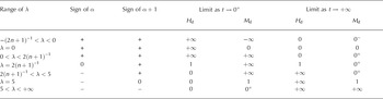
To understand the relation between the value of λ and the initial (t →0+) and ultimate (t →+∞) conditions of these similarity solutions, we non-dimensionalize t ~ t0, r ~ R0, H ~ H 0 and write Equation (10) as
in the new coordinates. Also
are dome height, margin radius and dome accumulation rate, respectively, in the non-dimensional coordinates.
From Equations (11) and (13) we have the various cases in Table 1.
Seeking only realistic solutions, we recall Equation (7), and note that if φ’(s) < 0 for some s > 0 then 3 > 0 and λ > —(2n + 1)–1. It follows that Rm (t) → 0+ as t → 0+ and Rm(t) →+∞ as t ! +1 A ‘delta function initial condition’ description is only appropriate for the solutions H A with — (2n + 1)–1 <A< 2(n + 1)–1; this range includes the Halfar A = 0 solution, of course.
Similarity solutions of Equation (3) for —∞ <A < – (2n + 1)–1 do exist. They satisfy φ’> 0 and β < 0. Equations (7), (8), (9), (10) and (12) must be changed appropriately. These solutions have infinite ice-sheet extent (thus R 0 is not defined) and infinite ice volume at all times. Flow is towards r = 0 into an interior ‘cup’ (except when β = 0, then thickness is constant in r). In any case, note that when A < 0 there is increasing ablation with increasing height. These curiosities are, perhaps, not useful for modelling or verification.
Figure 1 shows the profiles of H A for n = 3 at t = 0.110, t0 and 10t0 and for A = –1.7, 0 and 1.5. The A = 0 solutions have time-dependent volume;they are all new.
Three cases of the similarity solution (Equations (10) and (11)). (a) The Reference HalfarHalfar (1983) solution (A = 0) with constant volume and zero accumulation. (b) The A = –1/7 solution with height-dependent ablation and decaying volume; the margin does not advance. (c) The A = 1.5 solution with height-dependent accumulation and increasing volume; the margin advances rapidly.

An interesting similarity solution is obtained by setting A = 5. In this case the dome thickness Hd(t) grows linearly in time, from zero at t = 0, and the dome accumulation Md(t) for some sliding coefficient μ > 0. Various physical motivations for such laws exist (Reference MacAyealMacAyeal, 1989; Reference PatersonPaterson, 1994). Simple modification of the derivation below allows construction of exact solutions with basal sliding given by any reasonable function μb = F(τb). is constant as a function of time. Test C in section 3 is based upon this case.
The concatenated solution H = HA>5 for 0 < t < t 0 and H = HA<0 for t > t 0 forms a simple analytical ‘complete lifecycle’ model for an isothermal shallow ice sheet. It starts with zero ice and experiences a period of linear-in-surface-elevation accumulation. The accumulation switches off at t = t 0 (when A = 0) or switches to ablation (when A < 0) and the sheets decay to zero thickness as t →+∞. There is no discontinuity of H at t = t 0 because H A(r, t0) is independent of A.
2.2. Solution with basal sliding in an ice-stream-like region
In this subsection we show that compensatory accumulation functions can be defined to create essentially any profile we choose. The resulting exact solutions can be used, for example, to test the ability of numerical codes to deal with a spatially varying accumulation source term and/or basal sliding (for a broad range of sliding laws).
The Reference BodvarssonBodvarsson (1955)-Reference VialovVialov (1958) radially symmetric ice sheet with Vialov-Nye margin H = 0 at r = L and constant accumulation M 0 (Equation (17) below) is a well-known exact steady solution to the isothermal shallow-ice equation. In this subsection we construct an exact steady solution with basal sliding in an ice-stream-like sector, based upon the Bodvarsson-Vialov solution.
In particular, consider the equation
where q f is given by Equation (2) as before and ub is the basal sliding velocity, assumed proportional to a power p of the basal shear stress (τb = (τxz, τ yz) =—pgHVh in the shallow-ice approximation):
Our exact solution will have non-constant sliding parameter μ = μ(r, θ), in polar coordinates, varying continuously from zero in the regions of frozen base to a maximum μmax within the ice-stream-like region. In particular, we suppose the region is a sector q < r < r2, θ1 < θ < θ2, and we suppose such a sector appears in each quadrant of the ice sheet by reflection across x = 0 and y = 0. (Such symmetry produces a convenient verification test (see section 4) but is inessential to the derivation here.) Supposing r = L is the position of the margin, we require q > 0 and r 2 < L for non-singularity of certain quantities in what follows. In test E (section 3) we choose
within the region, and μ = 0 otherwise, for (relative) simplicity. Note that μ((q + r2)/2, (θ 1 + θ2)/2) = μmax.
Figure 2 shows the region of non-zero sliding and contours of the sliding parameter. Note θļ = 10, θ2 = 40, r1 = 200 km and r2 = 700 km, where L = 750 km in this map plane view; these are the parameters used in test E. The angles θ1 and θ2 have been chosen to produce a relatively generic sliding sector, not specially aligned to the finite-difference grid in section 4.
Contours of sliding parameter, μ, for an exact solution with basal sliding.

For the figures and for verification we choose p = 1 and μmax = 2.5 × 10⁻¹¹ Pa–1 ms–1. These values produce, for example, a velocity of 80 m a–1 at a basal shear stress of 100 kPa (1 bar).
To construct an exact solution to Equation (14) we find a compensatory accumulation Mb as follows. First, H(ŕ) is given by a predetermined function, in this case the Bodvarsson–Vialov profile
with M0 a positive constant. Now let
Then HV solves Equation (14) with M = M0 + Mb and u b given by Equation (15) with p = 1. This can be seen by substitution. Note that Mb is bounded and piecewise-differentiable but discontinuous; it is well known that discontinuous source terms pose no difficulties for diffusion equations (Reference EvansEvans, 1998).
The main point, however, is simply that HV is the exact solution to Equation (14) because Mb has been specifically chosen to make it so. Figure 3 shows H and M = M0 + Mb along the center line of the sector. The accumulation is greater than M0 upstream in the region, and is negative (ablation) downstream, in order to compensate for the basal sliding. That is, faster flow from basal sliding exports ice from the upstream region and piles it downstream; accumulation must compensate. Details of the calculation are addressed in the Appendix; test E in section 3 is based on HV and Mb.
Profile of ice thickness, H, (solid curve) and accumulation, M, (dashed curve) along the center line of the sector.

2.3. Time-dependent solution with compensatory accumulation
The technique used in section 2.2 to generate an exact solution with basal sliding has more general applicability. Many exact solutions suitable for testing, including the time-dependent solution we now describe, can be found this way. This solution, which has profile Hp (Equation (24)), is a perturbation of an apparently new steady-state solution Hs (Equation (21)). We construct a new steady solution because no existing smooth exact solution has its margin in an ablation zone. We seek a solution subject to a natural (ablation zone) boundary condition because, in the following verification test, margin drift is an indication of numerical error.
(Our derivation will produce a compensatory accumulation from the derivative of the flux, which therefore should be smooth. For the 2-D steady case there is an exact solution with piecewise constant accumulation/ablation (Reference PatersonPaterson, 1994, p. 245) which has been used in verification (Reference Calvo, Diaz, Durany, Schiavi and VazquezCalvo and others, 2002b), but that solution does not generalize to the radial case with a convenient expression.)
Thus, for the moment, we seek a steady radial solution to the isothermal shallow ice-sheet equation with margin at r = L situated in an ablation zone. With ![]() the scalar flux is
the scalar flux is ![]() Assuming
Assuming ![]() Integrating from an arbitrary radius r to a margin at r = L, where H(L) = 0, we have
Integrating from an arbitrary radius r to a margin at r = L, where H(L) = 0, we have
The purpose of this recapitulation is to note that an analytical expression for H(r) exists if the nth root of the flux function q(r) has an analytical integral. Thus we are invoking a technique for producing myriad steady analytical solutions. Note, however, that if r = 0 is in an accumulation zone and if the margin r = L is in an ablation zone then q(r) will grow linearly at r = 0 from a value of zero and will decay linearly at r = L to zero. One possible flux function q(r) with all of these properties is
for some C, where s = r/L. A dome thickness H0 at r = 0 determines ![]() The corresponding thickness function is
The corresponding thickness function is

where s = r/L. From Equation (20) we find an accumulation function Ms(r) = r–1 (d/dr)(rq(r)) by differentiation, that is,
Note Ms (0+) =2C/L and Ms (L—) = —C/L by limit arguments.
The particular functions Hs
and Ms
together form a new steady solution with dome in accumulation region and margin in ablation region (see Fig. 4). Both Hs and Ms
are smooth on 0 < r < L, and they satisfy 0 = Ms + ![]() exactly. They will be incorporated into test D in section 3.
exactly. They will be incorporated into test D in section 3.
The profile (solid curve) of a steady exact solution with margin in an ablation zone. Accumulation function shown (dashed) with location of equilibrium line noted. Dimensions and constants as in test D; see section 3.

We now return to the construction of an exact time-dependent solution. Suppose that we add to the steady profile H s a sinusoidal-in-time perturbation in the vicinity of the equilibrium line. Suppose, for example, a perturbation
if 0.3L < r < 0.9L, and P(r, t) = 0 otherwise; period of the perturbation and Cp its magnitude. Tp is the Let
Now, H = H p is an exact solution to the time-dependent equation
where hp = (1 – f)Hp. That is, one makes the constructed function Hp an actual solution to Equation (25) by
with compensating accumulation defined by
where hp = (1 – f)Hp. That is, one makes the constructed function Hp an actual solution to Equation (25) by with compensating accumulation defined by compensating with precisely that additional accumulation which makes it a solution.
Figure 5 shows thickness profiles and accumulation over one period Tp . Note that M is bounded but discontinuous because P has a continuous first, but not second, spatial derivative. During verification, the accumulation function is extended by –0.1 ma–1 in the region beyond the exact margin position so as to induce mild negative feedback for margin drift (see section 4).
(a) The envelope of Hp (Equation (24)), a perturbed steady solution. (b) The corresponding accumulations M = Ms + Mc (Equations (22) and (26)). Profiles are shown at t = 0, Tp/8,... 7Tp/8, that is, at eight equally spaced times in one period of the perturbation.
In a map plane view of the ice sheet the perturbation and corresponding non-zero values of Mc are confined to an annulus away from r = 0 and r = L. Because of the large variation of M over time, and because of the discontinuous nature of M, the resulting numerical verification test is quite challenging. Details of the calculation of Mc, as needed for test D in section 3, are given in the Appendix.
3. A Test Suite
We propose a verification suite for numerical ice-sheet codes based on exact, generally time-dependent, solutions. The five tests described here apply only to the isothermal-shallow-ice approximation. The exact solutions used in tests A (Reference BodvarssonBodvarsson, 1955; Reference VialovVialov, 1958) and B (Reference HalfarHalfar, 1983) appear in earlier literature. The remainder are new. This suite should be modified if more suitable exact solutions are found.
The tests include two steady-state solutions, one well known (test A) and one new (test E), while the remainder are time-dependent. They have flat beds (i.e. f = 0) and no basal sliding, with the exception of test E which has a linear basal sliding relation in a predetermined region.
The ice-sheet profiles in these tests are radially symmetric. Such solutions are challenging, in varying degrees, for numerical codes using rectilinear grids (finite-difference methods) or using adaptive triangulations (finite-element methods), because in either case the exact margin, as well as other contour lines, will not coincide with gridlines. A range of grid-orientation vs margin-orientation cases is thereby automatically tested.
A suggested verification mode for a time-stepping numerical scheme using the steady solutions (tests A and E) is:
exact thickness, H, is used as the numerical initial condition;
exact accumulation, M, is used at every step of the run;
after a run time sufficient to observe convergence to numerical equilibrium, errors are evaluated by comparing the computed thickness to the exact thickness.
A verification mode using the time-dependent solutions (tests B-D) is:
exact thickness, H, evaluated at the initial time, is used as the numerical initial condition;
exact accumulation, M, as a function of time and space, is evaluated at each gridpoint at every time-step;
at each time-step, t, errors are evaluated by comparing the computed thickness to the exact thickness at that time.
These modes of verification are illustrated in the next section.
Tables 2 and 3 detail the five tests. We have used the EISMINT I values of physical parameters when possible. The Glen exponent is n = 3 in all tests. The overall constant Г = 2A(pg)n/(n + 2) is determined from the EISMINT I values A = 10–16 Pa–3 a–1, g = 9.81ms–2 and p = 910 kg m–3, so that Г = 9.0177 × 10⁻¹³ m–3 s–1; there are 31 556 926 s a–1. The deformational flux qf is in every case given by Equation (2).
A test suite of exact solutions for verification of numerical isothermal ice-sheet models
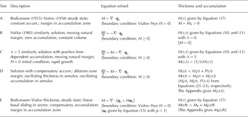
Continuation of Table 2: values of test parameters, comments and suggested uses

4. Verification of a Standard Numerical Model
In this section, we start by describing, for completeness and reproducibility, a standard and widely used numerical method for approximating isothermal shallow-ice flow, namely, an explicit finite-difference method. We then ‘run it through its paces’ with tests A-E. (This section is based on computations with MatlabTM programs placed in the public domain.)
There is good general agreement between exact and numerical solutions. There is clear evidence of convergence at all gridpoints in tests B–D, and for all interior gridpoints in tests A and E. Convergence is likely for all gridpoints in tests A and E. The particular difficulty of margin shape approximation, especially in regard to the Vialov–Nye case, is addressed in section 5.1.
A goal of this paper is to understand the nature and magnitude of numerical errors in a finite-difference method. Using our supply of exact solutions, we will report maximum errors and not the degree of agreement between different numerical approaches to the same problem. However, in section 5, we will also report the results of the same method on a sampling of the EISMINT I benchmarks and see that they are within the published range. We will then improve the EISMINT I benchmarks by estimating ‘exact’ results for the EISMINT I experiments using grid refinement and extrapolation.
4.1. Numerical method summary
The most general form of the equation of continuity considered in this paper is
where q f is given by Equation (2) and u b is given by Equation (15) with p = 1. For simplicity we use f = 0 so H = h.
We suppose a rectangular grid (xj, yk, t/) with fixed spacing ∆x, ∆y, ∆f. Let Hjy approximate H(xj, yk, tl) where H(x, y, t) is the exact solution to a particular initial/boundary-value problem. Our explicit finite-difference scheme for Equation (27) is

where, defining ![]() and recalling that μ is the spatially varying sliding coefficient,
and recalling that μ is the spatially varying sliding coefficient,

The quantity in square brackets in Equation (29) is the
numerical ‘diffusivity’. The staggered grid values of H and α
respectively, with appropriate modifications at the other staggered gridpoints. The ‘staggered grid’ flux Qy+1//2 is computed analogously. The deformational part of the Qx , Qy formulas is exactly as in Reference MahaffyMahaffy (1976) and is described as ‘type I’ in EISMINT I (see also Reference Hindmarsh and PayneHindmarsh and Payne, 1996).
To implement the natural boundary condition H > 0, tentative thicknesses Hj, k, l+1 are found from Equation (28)
using values at t = tl . If Hj, k, l+1 < 0 then Hj, k, l+1 is set to zero, otherwise the value is kept (Reference Hindmarsh, Greve, Ehrentraut and WangHindmarsh, 2001). In the case of a Vialov-Nye boundary condition, those gridpoints predetermined as outside the ice region are set as H = 0 at every time-step.
Overall dimensions -Lx < x < L x, -Ly < y < L y and run time T are supposed fixed. In our verifications the spatial domain is square so we suppose Lx = L y, N = Nx = N y, ∆x = 2Lx/N, ∆y = 2Ly//N and ∆t = T/K; there are (N + 1) gridpoints in each spatial direction.
Explicit methods, while easy to implement, are well known to be subject to stability restrictions (Reference Hindmarsh and PayneHindmarsh and Payne, 1996). To analyze numerical stability, one must temporarily linearize the problem. In particular, one must fix the diffusivity D =(1 - f)ГHn+21Vhn-1 at some time-step so that it no longer evolves in time. Steps of our explicit scheme for ∂H/∂t = M +V ■ (DVH) are then subject to the restriction (maxD)∆t/∆x2 < C for some constant Cof order one (Reference Morton and MayersMorton and Mayers, 1994). In a fixed total time run, a doubling of N therefore requires an increase in the number of time-steps Kby a factor of 4. On the other hand, the work of a run is proportional to N2K for this, and any other, explicit method. Therefore the work increases by a factor of 16 when N is doubled. Note that a fastest possible ‘refinement path’ (Reference Morton and MayersMorton and Mayers, 1994) in ∆x, ∆t space will therefore have ∆t ≈ C∆x 2 for some C’ (see Fig. 6).
Step sizes ∆t and ∆x used for each test; ‘refinement paths’. Values of ∆x correspond to N = 30, 60, 120 and 240 grids. Values of ∆t chosen as large as allowed by stability.

This restriction (max D)∆t/∆x2 < C does not directly apply to the actual (non-linear) evolution, but it has practical value. For instance, in test A we empirically determine C ≈ 0.15 from several runs while the linear stability analysis of Reference Hindmarsh, Greve, Ehrentraut and WangHindmarsh (2001) predicts that C = (2n)–1 = 1/6 from the slab flow. The restriction is reliable enough to be made the basis of an adaptive time-stepping scheme, though in this paper we used a fixed time-step in each run. Tests B and C would show distinct benefits of adaptation: in the first case, ∆t would lengthen as the sheet became shallower;∆t would shorten in the second as the sheet thickened.
To compute ice-sheet volume we have chosen the numerical method
This method is a reasonable choice because it is exactly the two-variable trapezoid rule. However, since H has unbounded gradient at a margin, all volume methods based upon polynomial approximation (trapezoid, Simpson’s, Gauss’...) will suffer from volume errors at the margin. The trapezoid rule at least makes minimal presumptions on differentiability.
It turns out that volume method (31) is compatible with the flux conservation of our explicit method and with our implementation of the H > 0 natural boundary condition. By ‘compatible’ we mean that this numerical scheme conserves Vnum to within the rounding error (less than one part in 1014) in accumulation-free cases. See the verification with test B below.
4.2. Verification and grid refinement study
Because the tests in this paper have radial symmetry, we have saved time by performing all computations in the quadrant 0 < x < L x, 0 < ỵ < L ỵ. (In test E there is symmetry of accumulation across both x = 0 and ỵ = 0.) We impose reflection boundary conditions along the lines x = 0, ỵ = 0; the origin (x, ỵ) = (0,0) is the center (‘dome’) of each ice sheet.
In each time-dependent test, the horizontal extent Lx = Lỵ was chosen large enough so that exact and numerical ice sheets never advance to within one gridpoint of the outside boundaries x = L x, ỵ = Lỵ of the computational domain. In particular, the natural boundary condition H > 0 in tests B-D was always imposed at gridpoints away from the x = L x, ỵ = Lỵ boundaries.
The runs were done with fixed ∆t, which was adjusted by hand to be close to the stability limit for the particular problem. From the grid refinement study we are convinced that, for time-dependent problems, choosing ∆t small enough to satisfy stability requirements makes the O(∆t) error of our first-order-in-time explicit method negligible relative to errors in spatial derivative approximations.
Runs using N = 30, 60, 120 and 240 were performed for each test;N = 30 is the EISMINT I choice and N = 60 is the EISMINT II choice. Figure 6 shows the refinement paths, in ∆t, ∆x space, used for each test.
Figures 7 and 8 summarize the results. We show maximum errors, i.e. max|Hnum – Hexact| over all gridpoints (x, ỵ) = (xj, ỵk) at the final time t = tf, and dome errors |Hnum(0, 0, tf) – Hexact(0,0, tf)| as functions of N, respectively. Best-fit lines, i.e. linear regression in (logN)× log(error) plane, and their slopes (‘O(N —p)’), are added to suggest the rate of convergence, discussed below.
Maximum error for each test; behavior of the errors under grid refinement. Errors for tests A and E are indistinguishable at this scale.

Dome error for each test; behavior under grid refinement.

Dome errors are surrogates for the ill-defined concept of ‘away-from-the-margin errors’. For example, Figure 9 shows contours of the errors for tests A and B with N = 60. The largest errors are confined to the vicinity of the margin, while error is relatively uniform and small in the interior. Dome errors are substantially smaller than maximum errors and they converge to zero faster. An explanation appears in section 5.1.
4.3. Further remarks on test A
Test A is a steady-state solution for which a run of 25 000 model years is sufficient for convergence to numerical equilibrium from the exact profile as an initial value (cf. EISMINT I). The error Hnum – Hexact therefore compares numerical to exact equilibrium.
We believe our numerical method is completely typical of EISMINT I (see section 5.3) but the maximum errors for test A in Figure 7 are larger than those suggested by figure 2 in EISMINT I. In EISMINT’s figure an error apparently on the order of 300m is shown at the last interior gridpoint (near the margin);only a 26m dome error is actually reported. (We necessarily refer to the EISMINT I 2-D results;three-dimensional (3-D) errors cannot be known without an analytical solution to the EISMINT I 3-D experiments.) As pointed out earlier, our radial tests are much more challenging than the EISMINT I steady-state experiment, in that circular margins are not aligned to the grid.
Figure 9a shows the spatial distribution of the error in test A. From Figure 7 we have a suggested O(N–0 33) rate of maximum error convergence. By contrast, the centered difference approximation of the V • qf term has O(N–2) local truncation error (found from Taylor’s theorem assuming four continuous derivatives (Reference Morton and MayersMorton and Mayers, 1994)), and thus the rate O(N–2) is the best possible global (discretization) error achievable by a numerical scheme using the centered formula. Note that in easier problems than ice flow, local errors tend to accumulate as one moves in from the boundary to give larger global errors. For ice flow with a grounded margin we see the opposite situation: errors are large near where H is exactly imposed (the boundary condition) and are small at the dome. In this case, unbounded derivatives obviously degrade the best behavior (see sections 5.1 and 5.2).
Spatial dependence of the errors in tests A and B when N = 60. Error is defined as Hnum – Hexact, which is positive everywhere using our type I scheme. Only one-quarter of the sheet is shown owing to symmetry. (a) Test A: maximum error of 650 m near margin; interior of sheet has errors in range 30–70m. (b) Test B: maximum error of 170 m near margin; interior of sheet has errors in range 1–5 m.

4.4. Further remarks on test B
Test B is the zero-accumulation similarity solution of Reference HalfarHalfar (1983), describing the spreading of a delta mass of ice driven solely by gravity. As shown in Figures 7 and 8, the errors are substantially smaller than in test A and converge to zero faster. They are smaller, in part, because the dome thickness at the final time is smaller (2283.4 m as opposed to 3600m), but primarily because the margin gradient singularity is milder (see section 5.1). Figure 9b shows the spatial dependence of the error at the final time when N = 60.
In Figure 10 we examine the numerical mislocation of the margin. We show gridpoints where the exact and numerical solutions disagree about whether ice is present at the final time. It turns out that, regardless of the value of N in test B, the width of the arc of mislocated-ice gridpoints is always three. That is, the arc can always be crossed by ‘stepping on’ at most three of them. We do not know the explanation for this particular number, but we may conclude that the method is doing an acceptable job of locating the margin. The location error is linear in ∆x, that is, O(N–1), while the O(N _0•39) thickness error near the margin decays much more slowly.
(a) Gridpoints on an N = 30 grid where the exact and numerical solutions disagree about whether ice is present at the final time in test B. (b) The corresponding result for N = 240. The arc is three gridpoints wide in both cases. The arc is also three gridpoints wide when N = 60 and N = 120 (not shown).

The exact solution in test B has constant volume over time. The finite-difference method used here also yields constancy of the numerical volume computed by Equation (31). Indeed, when the initial and final numerical volumes were compared, the absolute errors were 2, 0, 0.5 and 7m3 for N = 30, 60, 120 and 240, respectively. The numerically computed volume in question is approximately 4 × 10⁶ km3 and thus these errors are all smaller than 10–14 in a relative sense. Note that the numerical volume (Equation (31)) is not a perfect estimate of the exact volume. For instance, formula (31) approximated the exact (analytical) volume in test B only to within 0.07% for N = 60. Rather, the numerical choices made here (finite-difference method, numerical boundary condition and numerical volume method) are consistent in terms of volume conservation. Local volume conservation (flux conservation) for the finite-difference method is reasonably obvious;the property of our numerical scheme illuminated by this experiment is the (numerical) conservation of volume at the margin with a natural H > 0 boundary condition.
4.5. Further remarks on test C
Test C is a new non-zero-accumulation similarity solution with zero initial condition and linearly increasing dome height over time. The accumulation function has a constant (in time) maximum value of about 1.2 m a–1. Because M is proportional to H, the region of non-zero accumulation grows as the ice sheet advances.
Because diffusivity D depends on the n + 2 power of H, as thickness increases stability can ‘suddenly’ become an issue at some time-step. This test is therefore well suited to testing adaptive time-stepping (although we did no such test here).
The accumulation function M is irregular in the sense that it goes to zero with unbounded derivative at the margin. We use the final volume to measure the degree to which the numerical method accurately accumulates ice over time. The result is that the final numerical volume Vnum converges to the exact value at a relatively rapid O(N–2–41) rate.
In this paper, we have not taken full advantage of the verification opportunities offered by test C, namely, to verify a shallow numerical model of the ‘mass-balance altitude feedback effect’ (Reference Leysinger Vieli and GudmundssonLeysinger Vieli and Gudmundsson, 2004) in the case where accumulation is linear in surface height (thickness). In our tests we regarded the exact M(r, t) as a predetermined function of space and time. However, since M = \t –1H, one can instead compute the accumulation Mnum = 5t^Hnum at each gridpoint based on the approximate value Hnum. Such a calculation requires using the exact solution H(r, t) at positive t for an initial condition;an ice sheet of zero thickness does not grow if accumulation is linear in thickness.
4.6. Further remarks on test D
Test D is a time-dependent, sinusoidal perturbation of a new steady-state solution. After each period of Tp = 5000 model years the exact solution returns to the same thickness profile and thus to the same volume. It has margin in an ablation zone and the margin boundary condition is simply H > 0. The numerical margin is allowed to drift. We impose a 0.1 ma^1 ablation rate in the region outside the exact margin for mild negative feedback.
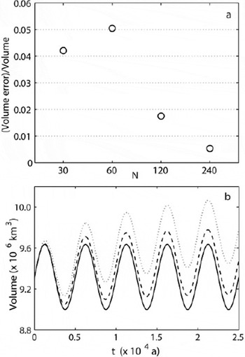
Now, because of oscillatory and irregular accumulation (Fig. 5), this test is ideal for measuring the degree to which the numerical method does not conserve volume. Figure 11a shows that as the grid is refined the numerical volume at the final time of 25 000 model years seems to converge to the exact value. Figure 11b shows the numerical and exact volumes over time; the N = 30 and N = 240 curves are omitted for clarity. Note, in particular, that no apparent phase error has occurred, and we believe this is because our time-steps are relatively small (for stability reasons).
Test D. (a) Relative volume error at 25 000 model years. (b) Exact (solid curve) and numerical volumes over time for N = 60 (dotted curve) and N = 120 (dashed curve).
4.7. Further remarks on test E
Test E is a steady-state solution which adds linear basal sliding and compensatory accumulation, in a sector, to test A (see Fig. 2). Again, a run of 25 000 model years was regarded as sufficient to produce numerical equilibrium, given the exact profile as an initial value.
The errors are maximum near the margin as in test A, and indeed dominate the error made in approximating basal sliding. We conclude that our numerical scheme for basal sliding is completely compatible, in terms of numerical difficulties, with difficulties already present in the frozen base case.
A contour map of the test E thickness error appears in Figure 12. It shows that the two processes of basal sliding and compensatory accumulation do, as designed, essentially cancel each other. By comparison with Figure 9a, we see that a slight asymmetry of the error contours, especially the 30 m contour, is the only visible indication of numerical non-cancellation.
Error Hnum – Hexact in test E with N = 60. Near-margin and interior errors are nearly identical to those in test A (cf. Fig. 9a). Compensatory accumulation and basal sliding essentially cancel as intended.

5. Discussion
5.1 On the approximation of margins
We now redo the regression on the maximum error graph (Fig. 7) by discarding the N = 30 case as an ‘outlier’. The result (Fig. 13) is that the three margin shapes - steady accumulation zone/Vialov-Nye (A and E), moving similarity/natural (B and C), and steady ablation-zone/natural (D) – determine the rates of convergence of the maximum error everywhere on the sheet. Unfortunately, we also see by the poor linear fit that for the Vialov–Nye margin cases (tests A and E) the rate of convergence may be slower than these linear fits suggest. It is conceivable, at least, that the error does not approach zero as O(N—p) for any p > 0, even in theory. In practice, it is clear that no achievable grid exists for our finite-difference method that would give a maximum error of, say, 50 m in test A. By contrast, a maximum error of 50 m is achievable in test B using N = 960, i.e. two more doublings of N = 240, if the convergence rate continues.
The convergence of maximum error is influenced by the type of boundary condition imposed. Here the linear regression is to the N = 60, 120 and 240 values only. Maximum errors in tests A and E coincide at the resolution of this figure.

The source of large maximum errors is the difficulty of numerically approximating ice-sheet margin shape. It turns out, in other words, that large maximum errors do not come from some elaborate non-linear mechanism or from the misapplication of numerical boundary conditions, but rather from the ‘simple’ issue of singular margin gradient.
Certainly the shallow approximation is invalid as a precise continuum description of ice flow as one approaches the margins, where neglected stress components become important. However, the shallow-ice approximation is both a good approximation for ice-sheet-scale behavior and is more practical at ice-sheet scales than the full system equations (Reference Leysinger Vieli and GudmundssonLeysinger Vieli and Gudmundsson, 2004), so the extent of disagreement between continuum solutions and their numerical approximations is important. In particular, we will explain why large numerical errors at margins do not ‘corrupt’ accuracy over the interior of the ice sheet.
The known (asymptotic) margin shapes correspond to three specific exponents. The mildest are ablation-zone steady margins with shape H(x) ~ x1/2 where x is a generic coordinate describing distance into the ice sheet from the margin (Reference FowlerFowler, 1997). (These are ‘mild’ in the sense that xp is of increasing differentiability at x = 0 as p increases.) The next mildest profiles appear in the similarity solutions H = Hχ of section 2.1. The shape is independent of the accumulation parameter χ: Hχ (x) ~ xn/(2n+Г). Finally, accumulation-zone steady margins (Vialov–Nye margins) have the steepest shape H(x) ~ xn/(2n+2) (Reference FowlerFowler, 1997).
We assume other time-dependent margin shapes are possible. We also suppose, however, that the xn/(2nþ2) power of a Vialov–Nye margin represents the most singular shape of interest to modellers.
The importance of these powers can be seen by evaluating the flux, given by Equation (2), as x →0þ, in these three cases. The result is that q(x) ~ x1, xn/(2n+1), x0, respectively. In the last case, q is not even continuous at x = 0 because, presumably, q(x) = 0 for x outside the ice.
All finite-difference methods which depend on the standard O(∆x2) centered-difference formulas for derivatives can be regarded as being implicitly based upon global piecewise linear approximation (although they are derived by Taylor series arguments). This can be seen clearly in certain examples, for instance, the perfect correspondence between the standard finite-difference and finite-element treatments of the simplest Poisson problem on a rectangle (section 1.2 of Reference JohnsonJohnson (1987)). Finite-element methods are, of course, explicitly based upon piecewise linear (or, at least, piecewise polynomial) approximations.
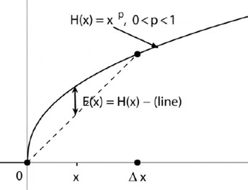
Consider the piecewise linear approximation of an ice-sheet margin with asymptotic shape H(x) = xp , 0 < p < 1, as in Figure 14. Suppose that a gridpoint coincides with the exact position of a margin. The next gridpoint is ∆x up-glacier and the error between the exact H and its linear approximation is E(x) =xp — (line) =xp—(∆x)p–1x. The maximum Emax = max E(x), for 0 < x < ∆x, is at x = ∆x • p1/(1— p) and has magnitude
for 7 = pp/(1—p) – p 1/(1—p). A more complete version of this analysis shows that even as the position of the last on-ice gridpoint is varied the approximation error is still O(N—p ).
Linear approximation of a margin H(x) = xp gives error E (x) = C (∆x )p .
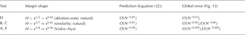
Our hypothesis is that Equation (32) predicts the numerical error in the vicinity of the margin, and thus the maximum error on the whole ice sheet (which we hypothesize always occurs at a point near the margin). Table 4 compares the prediction of this hypothesis to observed global maximum errors in the tests of section 4. The correspondence is close for the (steady) ablation-zone and similarity margins, but for the Vialov–Nye (steady) accumulation-zone margin the numerical errors are even larger than predicted by Equation (32). For natural margins there is a high-quality approximation of a continuum quantity evolving ‘in the background’, specifically of the transformed thickness η = H(2n+2’)/n , considered in section 5.2, and Equation (32) really determines the error. For the Vialov–Nye margin something is going wrong even for the η-evolution, namely that η is not continuously differentiable at the margin.
Margin shape predicts global error decay rate; Glen exponent n = 3
In any case, we believe this is strong evidence that margin shape, and not more optimistic local truncation error predictions from Taylor’s formula (e.g. Reference WaddingtonWaddington, 1981), controls the global discretization error in a shallow-ice-sheet simulation. As noted, such Taylor-series arguments predict O(N–2) local error which accumulates as one moves in from the margin.
5.2. Regularization of the margin by a transformation
Following Reference Calvo, Diaz, Durany, Schiavi and VazquezCalvo and others (2002b), we let η = H(2n+2)/n for Glen exponent n. Equations (1) and (2), with u b = 0 and f = 0 for simplicity, are equivalent to for Г = [n/(2n + 2)]nГ. Equation (33), with its natural boundary condition η > 0, describes an evolution equivalent to the original ice equation.
The η-margin is much less steep than the H-margin. To see this, let n = 3 for simplicity. Margin shapes H(x) ~ x1/2, x317 and x3/ŭ are transformed to η(x) ~ x4/3, x877 and x1,
The n-margin is much less steep than the H-margin. To see this, let n = 3 for simplicity. Margin shapes H(x) ~ x 1/2, x 3/7 and x 3/8 are transformed to Z(x) ~ x 4/3, x 8/7 and x 1 respectively. That is, the ablation-zone steady and similarity margins are transformed to functions η with continuous derivative. The accumulation-zone (Vialov-Nye) margin is transformed to a η-margin with bounded but discontinuous derivative. For illustration, the η-analog of the Reference HalfarHalfar (1983) solution, that is, the 8/3 power of Hλ (r, t) in Equation (10) with λ = 0, is shown in Figure 15.
Profiles of η for the λ = 0 similarity solution at times t0 (dotted curve) and 3t0 (solid curve). Note there is no discontinuity of ∂η/∂r at the margin; shape is η = x8/7 if x is distance from margin. (Cf. Fig. 1a.)

We rerun test B doing the calculation in terms of η. The numerical method used for η (Equation (33)) is the direct analog of the explicit finite-difference method described in section 4.1. Figure 16 shows the rate at which the (relative) maximum and (relative) dome errors converge as N increases. (‘Relative maximum’ error is ‘relative to the value of η at the dome’.) For the evolution of η the maximum error and dome error now decay at comparable rates. The maximum error goes to zero at rate O(N–1•07), instead of O(N–0Л4) for H, because the η-margin is well behaved. The significance of this good performance is, we believe, that errors in H are much greater near the margin than in the interior only because H is the 3/8 power of η and not because of more complicated non-linear effects. The convergence rate of the H dome thickness closely matches that of η. ‘Corruption’ from margin errors does not extend into the interior for either the H or η computation, except to reduce the order of interior convergence from the best conceivable rate O(N–2) to about O(N–15).
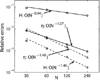
5.3. Methods for improving the EISMINT benchmarks
Having verified our numerical method relative to exact solutions, we consider the continuum problems used by EISMINT as benchmarks. An important criticism of EISMINT I is that the values reported as benchmark results are not numerical results of ‘benchmark quality’. For several examples of benchmark-quality results for problems in fluid dynamics without an analytical/exact solution, see Reference RoacheRoache (1998). We will show how such benchmark-quality results can be extracted for these particular problems. Nonetheless, for verification the use of exact solutions is easier and the sources of error are more understandable than if benchmark-quality numerical solutions are used.
We have reproduced three of the six EISMINT I experiments, namely the ‘fixed-margin experiment in steady state’, the ‘fixed-margin experiment forced by sinusoidal boundary conditions with a period of 20 kyr,’ and the ‘moving-margin experiment in steady state’, to show how the benchmarks can be improved upon. We compute on the EISMINT I grid with N = 30 and then on refined grids with N = 60, N = 120 and N = 240.
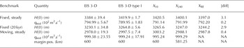
Table 5 reports the EISMINT I results and our results for dome/divide thickness H(0), ‘midpoint’ flux (which is at 400 km away from the dome;the margin in the fixed case is at position 750 km) and margin position itself (in the moving-margin experiment). The table gives the EISMINT I 3-D value and range, that is, the mean and standard deviation of the 11 results from 3-D codes, and also the value and range of results from those five codes which, like ours, use ‘type I’ diffusivity/flux finite-difference approximations. We report our results on the N = 30 and N = 240 grids (‘X30’ and ‘X240’);though N = 60 and N = 120 results were calculated, they are omitted from the table for clarity. In each case our N = 30 values are in the EISMINT type I range.
A sampling of EISMINT I benchmarks values (columns 3 and 4), our values on the N = 30 rough grid (column 5) and versions improved by grid refinement and Richardson extrapolation (columns 6 and 7). See section 5.3 for last column
Consider the dome/divide thickness H(0) in the fixed-margin and steady case. There exists a correct value for the continuum problem; unfortunately the EISMINT I square geometry means that it is not known analytically. However, we can use grid refinement and Richardson extrapolation (Reference Burden and FairesBurden and Faires, 2001) to get a much more accurate estimate than from the N = 30 grid, or indeed from any fixed grid. Figure 17 shows H(0) values from the N = 30, 60, 120 and 240 grids. These are associated with decreasing values of ∆x, of course. Following the technique of Richardson extrapolation, we suppose that the numerical approximation to H(0) is a polynomial function of ∆x; the convergence results of section 4 suggest limited validity to this assumption as dome errors converge as O(∆xq) for 1 < q < 2 (Fig. 8). We nonetheless choose the degree of that polynomial to be two (and ignore the N = 30 case;see Fig. 13).
Richardson extrapolation gives a better estimate of the correct dome/divide thickness for the EISMINT I fixed-margin, steady-state experiment.

Using data for three values of ∆x (N = 60, 120 and 240), we find the coefficients a, b and c in X = a + b∆x + c∆x2 where X is the computed quantity. Evaluation of this polynomial X(∆x) at the ultimately refined grid spacing ∆x = 0 gives the Richardson extrapolation value reported in the table as ‘XRE’ and shown in Figure 17. The column ‘|diff|’ in Table 5 gives values of |X240 - XRE|. Richardson extrapolation does not come with an error bound, but this difference is a (probably conservative) estimate of the precision of XRE.
Two details in Table 5 require comment. First, the position of the margin in the moving-margin experiment is a discrete quantity and extrapolation is not appropriate. The exact (analytical) value is available, 579.81 km, and our N = 240 value (581.25 km) is, as expected, better than the EISMINT I value of 600 km. Second, the midpoint flux value in the moving-margin experiment did not behave with sufficient regularity under grid refinement to produce a good extrapolation. This value is sensitive to discrete jumps of margin position. These cases show some of the limitations of Richardson extrapolation of numerical results for producing benchmark values, but codes can nonetheless be tested against such extrapolated results if relevant exact solutions are not available.
6. Conclusions
Exact solutions do exist and are sufficiently diverse to allow verification of numerical codes for isothermal, shallow-ice-sheet models. Such verification completely avoids the rough grid intercomparison performed by EISMINT I. Indeed, it avoids creating uncertain benchmark values from numerical approximations. We hope that the ideas here serve as a refoundation of the EISMINT effort, which has proceeded with validation and verification of thermocoupled shallow-ice-sheet models (EISMINT II) and other ‘Phase II’ models.
Grid refinement shows that the explicit finite-difference numerical scheme of this paper substantially succeeds in recovering time-dependent continuum results in cases for which we have exact solutions. Other numerical schemes should, of course, succeed as well. Grid refinement also gives an estimated rate of error decay as N increases. Such rates potentially allow the choice of a grid which produces a given accuracy on a class of problems similar to an accomplished verification.
A widely noted difficulty became quantitatively clear in our verification process: margins are difficult to approximate. Margin shape from the shallow approximation is always a sufficiently singular function so that a numerical method based on piecewise polynomial approximation (thus any finite-difference or finite-element method) makes substantial errors near the margin. Indeed, the rate of decay of the maximum thickness error anywhere on the ice sheet is essentially predictable from the margin shape. Vialov-Nye margins are particularly difficult to approximate. Generally, however, errors in margin approximation do not seriously corrupt the accuracy of numerical approximation in the ice-sheet interior (in the isothermal case, at least).
Acknowledgements
Thanks to M. Truffer and R. Warner for their interest, to R. Hindmarsh and two anonymous referees for redirecting our efforts, to C. Dawson for reminding the first author of a ‘trick,’ and to the NASA Cryospheric Sciences Program for support from grant NAG5-11371.
Appendix: Calculation of Compensatory Accumulations
From section 2.2, and as further specified in test E, the Bodvarsson-Vialov steady solution can be made into a solution to a steady equation with basal sliding by adding a compensatory accumulation
We use f = 0 in test E. Denoting δ/δr = (•)0, recall that V • (ar) = r–1 (ra)0. Thus
Let ![]() and
and ![]() From test
From test ![]() The derivative terms needed to calculate M
b are as follows:
The derivative terms needed to calculate M
b are as follows:
and μ’ = 0 except that for η < r 1 < r 2 and θλ < θ < θ 2,
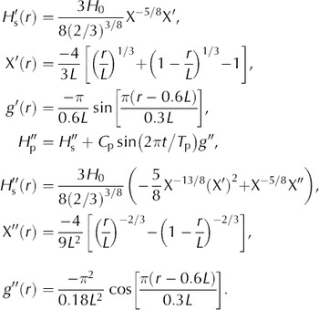
From section 2.3, and as further specified in test D, a perturbation of a steady solution can be made into an exact time-dependent solution by calculating the compensatory accumulation (Equation (26)):
The thickness Hp is given by Equation (24). In the case n = 3 and f = 0, as in test D, further details are as follows.
For 0 < r < 0.3L and r > 0.9L, P(r, t) = 0 for all t. The compensating accumulation is
For ![]() then the three terms of M
c are:
then the three terms of M
c are:
M s as Equation (22);
Note ![]() where
where ![]() From Equation (21)
From Equation (21)
where
Thus we need