2.1. Apparatus

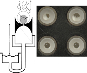
Our experimental apparatus is shown in figure 1(a). It consisted of a 9.5 mm (inner diameter) Perspex tube of 10 cm length, connected by a polyvinyl chloride tube to a 50 ml reservoir. The inner diameter at the upper end of the Perspex tube was increased to 12.5 mm to accept a bead holder machined from polyoxymethylene (trade name Delrin), which is shown black in the figure. It consisted of a 3.86 mm deep approximately half-spherical indentation with a 2 mm diameter hole at its lowest point. During the experiment, the hole connected the hydrogel bead via a continuous water column to the reservoir. Therefore, the distance between the hydrogel bead and the reservoir determines the sub-atmospheric pressure $P=P_a - \rho g H$ under the bead, where $P_a$ is atmospheric pressure, $\rho$ is the density of water, $g$ is the acceleration due to gravity and $H$ is the hydraulic pressure head. The remainder of the bead surface was exposed to the surrounding atmosphere, allowing evaporation.

Figure 1.

Schematic of the apparatus used for the experiment. (a) Detailed view of an individual bead holder with reservoir assembly. We approximate the bead as a sphere of diameter $d$, while the actual form (for the upright state) is shown with a dotted outline. (b) Evaporation chamber assembly – four (only two visible) of the bead holders shown in (a) were inserted into a cylindrical evaporation chamber. Note the humidity sensors at inflow and outflow. Conditioned air is delivered by the bubbler assembly shown in (c). The photograph (d) shows the hydrogel beads as seen by the camera. The deformation associated with the experiment makes larger beads unstable, which causes them to fall over (on-side state). Larger pressure heads cause smaller beads to remain in the upright state.

We controlled the atmospheric conditions around the beads by inserting four of these tubes into an evaporation chamber of approximately 6 cm diameter and 5 cm height as shown in figure 1(b) (only two tubes are visible). The four tubes were arranged in a square with a centre-to-centre distance of approximately 2.5 cm as shown in figure 1(d). The top of the chamber was sealed with a circular glass plate, 50 cm above which was an SLR camera used to monitor the changes in diameter $d$ of the hydrogel beads. A typical image is shown in figure 1(d). The four reservoirs were mounted on vertical rails so that the pressure heads could be changed easily.

The atmospheric conditions in the evaporation chamber were controlled by continuously purging it with air of relative humidity $\mathcal {RH}_i$ and flow rate $\mathcal {Q}$. The air entered through two ports in opposite side walls and left through a single port. The figure shows only two inlets and two outlets. The relative humidity $\mathcal {RH}_o$ of the outflow was measured to determine the evaporation rate, as described below.

Air of defined relative humidity was generated by bubbling air through saturated salt solutions (Greenspan Reference Greenspan1977; Wedler Reference Wedler2004) using the apparatus illustrated in figure 1(c). The first flask contained pure water to saturate the air, while the second and third flask contained the salt solutions required to set the desired relative humidity. A full list of salt solutions is provided in the supplementary material available at https://doi.org/10.1017/jfm.2021.608. A second air pump (see figure 1b) was used for the dataset shown in figure 3 to increase the air velocity in the evaporation chamber without changing the relative humidity.

The procedure for calibration of the sensors and correction of other minor differences between the set-ups used in different experimental runs is described in the supplementary material.

2.2. Procedure

In these experiments, it is important that no air bubbles interfere with the flow of water from the reservoir to the bead. For each bead holder, the reservoir was initially placed such that the bead holder held a small pool of water. A saturated ionic hydrogel bead (poly[acrylamide-co-(potassium acrylate)] more details in the supplementary material) was then placed in the pool to cover the hole and the reservoir was lowered to the desired height. There was sufficient contact between the bead and the rim of the hole to prevent air being drawn into the system by the negative pressure head below the bead. Excess water was carefully removed with a tissue, and the remaining water around the bead evaporated after a few hours. The beads then shrank until a steady state was reached. Our standard procedure was initially to flush the chamber with air at $\mathcal {RH}_i \approx 0.43$ and ${\mathcal {Q}}=0.65 - 1.0\ {\rm l}\ {\rm min}^{-1}$, which led to the first steady state after four to five days.

After the first steady state was reached, we explored the response of the beads to variations in $\mathcal {RH}_i$, $\mathcal {Q}$, the air velocity in the humidity chamber and the pressure head $H$. The datasets used in this paper are summarised in table 1. The full datasets are provided with further explanations in the supplementary material.

Table 1.

Overview of the datasets included. The size $d_0$ of the saturated bead was determined after the experiment. The time-resolved data of D, E and F are provided in the supplementary material.

2.3. General observations

More than half of the beads did not reach a steady state but dried out within a few days. We attribute this to a compromised seal between the hydrogel and the bead holder, which allowed an air bubble to form beneath the bead, drastically decreasing the availability of water. Even if the beads reached the first steady state, beads often dried out at later stages for no apparent reason. This unresolved problem with the experiments is a consequence of the fact that the hydrogel is not constrained but free to change its size and shape. For some experiments, we attempted to reset these beads by lifting the reservoir so that the air was pushed out from below the bead holder; this is indicated in the appropriate table.

A typical image of beads in steady state is shown in figure 1(d). Although whole beads or parts thereof appear dark, they actually remain transparent. The dark regions are due to the projection of the hole in the bead holder onto the bead surface. Changes in this projection could sometimes be used to determine whether air had accumulated under the bead. We also observed that larger beads tended to appear moist (shiny), while smaller beads in steady state appeared dry (dull).

Figure 1(d) is representative of the two distinct configurations found for the hydrogel beads in steady state. The top row shows an on-side configuration. The beads are slightly elongated and seem to have fallen over. The bottom row in the figure shows beads in an upright state. These beads are also slightly elongated but sit upright in the bead holder. We observed that larger pressure heads $H$ (i.e. lower pressure under the bead) tended to give rise to the upright state. We were unable to investigate this systematically but discuss it further in the context of § 2.4.3 below.

When experiments were terminated with beads still in steady state (i.e. had not dried out), a small dimple was found where the beads were in contact with water through the hole in the bead holder. The dimple disappeared within approximately ten minutes of removing the bead from the holder and appeared to be more pronounced for beads in the upright state. We therefore believe that the larger pressure heads pulled the bead into the bead holder, stabilising the upright state.

We note that the saturated bead sizes after the experiment reported in table 1 are larger than the average bead sizes reported in the supplementary material, probably because the hydrogel beads for the experiments were chosen with a bias towards the largest swollen beads available. Slower relaxation processes could occur which alter the swelling properties when the beads remain swollen for a long time. An indication of this is that the beads received from the manufacturer are clear, while swollen and subsequently dried beads become turbid and are of yellowish colour.

3.1. Constitutive equation for transport

Relative motion between the constituents of an aqueous binary system can be described by Darcy's law

(3.2)\begin{equation} \eta \boldsymbol{u} ={-}K\nabla p, \end{equation}

where $\boldsymbol u$ is the volume flux of water relative to the polymer skeleton (see below), $\eta$ is the dynamic viscosity of water and $K(\phi )$ is the permeability of the medium, which is a function of the porosity $(1-\phi )$  where $\phi$ is the volume fraction of polymer in the gel. This is equivalent to equation (17) of Bertrand et al. (Reference Bertrand, Peixinho, Mukhopadhyay and MacMinn2016). Our formulation, which follows Peppin et al. (Reference Peppin, Elliott and Worster2005), leads us to associate the pervadic pressure with the pore pressure that drives flow through the medium.

3.2. Constitutive relation for osmotic pressure

The polymer that forms the skeleton of a hydrogel is soluble in water but is prevented from dispersing completely by cross-links between polymer chains. The strands of polymer between cross-links act as (entropic) springs. Our one-dimensional model considers only isotropic stresses (pressures). Thus, at any point $z$, we express the total pressure as

(3.3)\begin{equation} P = {\rm \pi}+ p_e +p, \end{equation}

where ${\rm \pi} (\phi )$ is the osmotic pressure of solution (due to mixing of polymer and water) and $p_e(\phi )$ is a contribution to the total pressure from internal elasticity. This arrangement highlights the fact that the total mechanical pressure $P$ on the gel is given by the sum of the pervadic pore pressure $p$, the elastic pressure $p_e$, sometimes called the effective pressure of a porous medium especially in the context of soil science, and the osmotic pressure of solution ${\rm \pi}$. Note that in a three-dimensional description a constitutive equation for the Cauchy stress tensor is required, where $p_e+{\rm \pi}$ is the isotropic part of Terzhagi's effective stress tensor and $P$ the isotropic part of the Cauchy stress tensor.

The constitutive equation (3.3) is expected to have the general property that ${\rm \pi} (\phi )$ is an increasing function of $\phi$ (the swelling pressure is large when the polymer fraction is high) and that $p_e(\phi )$ is negative with magnitude decreasing with increasing $\phi$ (the stretched polymer strands are in tension). It is common to obtain ${\rm \pi}$ from Flory–Huggins theory and to use an expression obtained from a polymer chain model for $p_e$ (Tomari & Doi Reference Tomari and Doi1995; Hong et al. Reference Hong, Zhao, Zhou and Suo2008; Doi Reference Doi2009; Chester & Anand Reference Chester and Anand2010; Engelsberg & Barros Reference Engelsberg and Barros2013; Bertrand et al. Reference Bertrand, Peixinho, Mukhopadhyay and MacMinn2016).

Given the simplifications we have already made, we avoid the complexity introduced by the aforementioned references and use simplified expressions which represent the key properties mentioned above. We therefore take Flory–Huggins theory in the limit of small polymer volume fraction for ${\rm \pi}$ (also known as van't Hoff's law), which yields ${\rm \pi} = {\mathcal {A}}\phi$. In our model, $\mathcal {A}$ sets the magnitude of the osmotic pressure. For a hydrogel with charged groups, as we use in our experiments, the magnitude of $\mathcal {A}$ is likely to be determined by ionic effects and may be larger than for an uncharged polymer (see e.g. Tanaka et al. Reference Tanaka, Fillmore, Sun, Nishio, Swislow and Shah1980, for the osmotic pressure of an ionic gel). To avoid issues in the limit of large swelling (as pointed out by Chester & Anand Reference Chester and Anand2010), we chose a simple expression for $p_e$, which we only require to diverge for large swelling, consistent with our physical expectation. Our choice is $p_e=-k/\phi ^{2/3}$, but the precise detail of this is, eventually, immaterial owing to the steps that follow.

We use as a reference state the equilibrium in which the hydrogel is immersed in water at atmospheric pressure, so that $P=p = P_a$ and the equilibrium polymer volume fraction is $\phi _0$, in which case

(3.4)\begin{equation} \phi = \phi_0 \equiv \left(\frac{k}{\mathcal{A}}\right)^{3/5}. \end{equation}

For small departures from such an equilibrium, we use the leading-order Taylor expansion

(3.5)\begin{equation} P-p \approx A(\phi - \phi_0)={\rm \pi}_0\frac{\phi-\phi_0}{\phi_0}, \end{equation}

where $A = 5{\mathcal {A}}/3$ and ${\rm \pi} _0=A\phi _0$ corresponds to the osmotic modulus (Doi Reference Doi2009). In general, ${\rm \pi} _0 = \phi ({\partial }/{\partial \phi })({\rm \pi} + p_e)|_{\phi =\phi _0}$ with $\phi _0$ being the root of ${\rm \pi} (\phi ) + p_e(\phi ) = 0$. Note that ${\rm \pi} _0$ describes the combined effect of mixing and stretching of the polymer chains around the fully swollen state.

3.3. Transpiration flow

We consider one-dimensional flow of water through hydrogel of height $a(t)$ placed on a fixed water-permeable membrane at $z=0$, evaporating at the surface $z=a(t)$ with prescribed flux $q(t)$, as shown in figure 6(a). The region $z<0$ is filled with liquid water, which enters the hydrogel via the membrane with derived flux $u_0(t)$. The bulk pressure $P$ is equal to atmospheric pressure $P_a$ at the surface $z=a$ and to the reduced pressure $P_a - \rho g H$ below the membrane at $z=0-$. We present a fluid-mechanical model to determine the concentration of polymer $\phi (z, t)$ and the height of the gel $a(t)$.

3.3.1. Governing equations

The evolution of this system is very slow and so we neglect inertia. For simplicity, we also assume (reasonably) that the polymer and water have equal densities $\rho$ in pure and mixed state. Therefore, mechanical equilibrium gives

(3.6)\begin{equation} \frac{\partial P}{\partial z} ={-}\rho g \ \Rightarrow \ P = P_a + \rho g (a-z). \end{equation}

Note that $P(z=0+)=P_a +\rho g a$, which is greater than the pressure $P_a-\rho g H$ in the liquid beneath the semi-permeable membrane at $z=0-$. The resultant force is balanced by the rigidity of the membrane in our model and the bead holder in our experiment.

We assume ideal mixing so that both mass and volume of polymer and water are conserved locally. The continuity equations for polymer and water are therefore

(3.7a,b)\begin{equation} \frac{\partial \phi_w}{\partial t} + \frac{\partial (\phi_w u_w)}{\partial z} = 0 \quad\mathrm{and}\quad \frac{\partial \phi}{\partial t}+\frac{\partial (\phi u_p)}{\partial z}=0 , \end{equation}

where $\phi _w=1-\phi$ is the volume fraction of water, $u_w$ and $u_p$ are the water and polymer velocities and $t$ denotes time. Summing these equations, noting that $\phi _w + \phi = 1$ is independent of time, and then integrating with respect to $z$, we find that

(3.8)\begin{equation} (1-\phi) u_w + \phi u_p = q_0, \end{equation}

given that at $z=0$ the polymer velocity $u_p$ is zero and the water flux $(1-\phi ) u_w$ is equal to the flux of water entering from below the membrane $q_0(t)$. This expression can be rearranged to show that the polymer velocity is

(3.9)\begin{equation} u_p = q_0 - u, \end{equation}

where the Darcy flux $u \equiv (1-\phi )(u_w - u_p)$ is the volume flux of water relative to the polymer skeleton of the hydrogel. Hence, (3.7a,b) can be written as

(3.10)\begin{equation} \frac{\partial \phi}{\partial t} = \frac{\partial }{\partial z}[\phi (u-q_0)]. \end{equation}

This hyperbolic nonlinear equation is a conservation equation for polymer, which is coupled to Darcy's equation (3.2) for the relative water flux, which can be written as

(3.11)\begin{equation} u = \frac{K(\phi)}{\eta}\left(\frac{{\rm \pi}_0}{\phi_0}\frac{\partial \phi}{\partial z} + \rho g\right), \end{equation}

using (3.5) and (3.6). Equations (3.10) and (3.11) can be combined to give a nonlinear advection–diffusion equation for the polymer concentration

(3.12)\begin{equation} \frac{\partial \phi}{\partial t} + q_0\frac{\partial \phi}{\partial z} = \frac{\partial}{\partial z}\left[\frac{\phi K(\phi)}{\eta}\left(\frac{{\rm \pi}_0}{\phi_0}\frac{\partial \phi}{\partial z} + \rho g\right)\right] \end{equation}

but the physics is perhaps more clearly represented by the separate (3.10) and (3.11).

Note that there is a static equilibrium, which can be achieved by maintaining the atmosphere above the hydrogel bead fully saturated, in which ${\partial \phi /\partial z} = -\rho g /A$ is negative: the polymer concentration decreases slightly upwards to provide a generalised osmotic pressure gradient that balances the force of gravity.

The equations are completed with a specification of the permeability $K(\phi )$. It is common to use expressions similar to the Kozeny–Carman equation, such as $K(\phi ) \propto (1-\phi )^3/\phi ^\beta$, with various values of $\beta$ suggested in different contexts. In Appendix A.1, we argue that the appropriate value for hydrogels, given conservation of polymer, is $\beta = 2/3$. For now we choose a general expression but make use of the fact that $\phi \ll 1$ to approximate

(3.13)\begin{equation} K(\phi) = K_0\left(\frac{\phi_0}{\phi}\right)^{\beta}, \end{equation}

where $K_0$ is the permeability of the swollen gel.

3.3.2. Boundary conditions

By definition, the pervadic pressure $p$ is continuous across the semi-permeable membrane at $z=0$, and it is equal to the bulk pressure $P=P_a - \rho g H$ in the liquid just below the membrane $z=0-$. Therefore, using (3.5) and (3.6) we determine that the polymer concentration satisfies the Dirichlet boundary condition

(3.14)\begin{equation} \phi = \phi_0\left[1 + \frac{\rho g}{{\rm \pi}_0}(H+a)\right] \quad (z=0). \end{equation}

At the upper surface of the bead, the relative flux of water through the gel is equal to the evaporation flux, $u=q$, so the polymer concentration satisfies the Neumann boundary condition

(3.15)\begin{equation} u=\frac{K(\phi)}{\eta} \left(\frac{{\rm \pi}_0}{\phi_0}\frac{\partial \phi}{\partial z} + \rho g\right) = q \quad (z=a (t)). \end{equation}

An additional constraint is needed to determine the unknown boundary position of the hydrogel surface, $z=a(t)$. This is obtained from an expression for the conservation of polymer in the hydrogel bead. Here, we make the approximation of isotropic expansion of the hydrogel to give

(3.16)\begin{equation} a^2\int_0^a\phi\,\mathrm{d}z = \phi_0a_0^3 \end{equation}

to use our one-dimensional model to reflect more closely the three-dimensional swelling and de-swelling observed experimentally. This is an important dimensional consideration in order to obtain appropriate orders of magnitude for the polymer volume fraction, and hence the pore size relevant to the permeability, used in Darcy's equation for the flow.

Equation (3.12) also requires an initial condition. An example would be to start with a bead taken from an equilibrium state immersed in water (in which it is neutrally buoyant by assumption that the densities of water and polymer are equal), in which case $\phi \equiv \phi _0$ and $a = a_0$.

3.4. Non-dimensionalisation

We introduce non-dimensional variables,

(3.17a–d)\begin{equation} \tilde{\phi}=\frac{\phi}{\phi_0},\quad \tilde{u} = \frac{u\tau}{ a_0},\quad \tilde{z}=\frac{z}{a_0}, \quad \tilde{t}=\frac{t}{\tau}, \end{equation}

where the poroelastic time scale is

(3.18)\begin{equation} \tau = \frac{a_0^2\eta}{K_0 {\rm \pi}_0}. \end{equation}

The complete problem in non-dimensional quantities is then

(3.19a)$$\begin{gather} \frac{\partial \tilde{\phi}}{\partial \tilde{t}} + \tilde{q_0} \frac{\partial \tilde{\phi}}{\partial \tilde{z}} = \frac{\partial }{\partial \tilde{z}}(\tilde{\phi}\tilde{u}), \end{gather}$$

(3.19b)$$\begin{gather}\tilde{u} = \tilde{\phi}^{- \beta}\left(\frac{\partial \tilde{\phi}}{\partial \tilde{z}} + \epsilon\right), \end{gather}$$

with boundary conditions

(3.20a)$$\begin{gather} \tilde{\phi} = 1+\tilde{H} + \tilde{\epsilon} \quad (\tilde{z} = 0), \end{gather}$$

(3.20b)$$\begin{gather}\tilde{u} = \tilde{q} \quad (\tilde{z} = \tilde{a}), \end{gather}$$

(3.20c)$$\begin{gather}\tilde{a}^2\int_0^{\tilde{a}(t)}\tilde{\phi} \,\textrm{d}\tilde{z} = 1 \end{gather}$$

and initial condition

(3.21)\begin{equation} \tilde{\phi} = 1 \quad (\tilde{t} = 0). \end{equation}

The dimensionless parameters in this system are the dimensionless evaporative flux

(3.22)\begin{equation} \tilde{q} = \frac{a_0 \eta}{K_0 {\rm \pi}_0}q, \end{equation}

the dimensionless pressure head

(3.23)\begin{equation} \tilde{H} =\frac{\rho g}{{\rm \pi}_0}H, \end{equation}

and the dimensionless head associated with the bead

(3.24)\begin{equation} \tilde{\epsilon} =\frac{\rho g a_0}{{\rm \pi}_0}. \end{equation}

In our experiments, we have seen changes in $\tilde {a}$ of several tenths (order unity) related to evaporation rates $q\approx 10^{-7}\ {\rm ms}^{-1}$ or pressure heads $H\approx 10$ cm. We therefore require that $\tilde {q}$ and $\tilde {H}$ are of order unity but, given that $a_0\approx 1$ cm, we assume $\epsilon \ll 1$ and neglect it in the subsequent analysis.

These observations also allow us to estimate some of the physical parameters of our experimental system. If $\tilde {H}\approx 1$ when $H\approx 10$ cm then (3.23) gives ${\rm \pi} _0 \approx 10^3\ {\rm Pa}$, given $\rho \approx 10^3\ {\rm kg}\ {\rm m}^{-3}$ and $g\approx 10\ {\rm m}\ {\rm s}^{-2}$. If $\tilde {q}\approx 1$ when $q\approx 10^{-7}\ {\rm ms}^{-1}$ then (3.22) gives $K_0\approx 10^{-15}\ {\rm m}^2$, given $a_0\approx 1$ cm and $\eta \approx 10^{-3}\ {\rm Pa}\ {\rm s}$. This permeability corresponds to a pore size of approximately 300 nm. This is based on the estimate that for many natural porous media the length scale $l$ is related to the permeability $K$ by $l^2\approx 10^2 K$. For example, Cubaud & Ho (Reference Cubaud and Ho2004) find $l^2=28.43K$ for square channels. This estimate of permeability and corresponding pore size appears reasonable, as Gombert et al. (Reference Gombert, Roncoroni, Sánchez-Ferrer and Spencer2020) report hierarchical structures in polyacrylamide hydrogels with features up to 100 nm size.

Finally, (3.18) gives an estimated time scale of $\tau \approx 10^{5}$ s, which is approximately 1 day, consistent with our experimental observations. These estimates will be refined below using comparisons between our theoretical predictions and experimental results.

3.5. Steady states

Steady-state solutions to (3.19) with $\beta =2/3$ can be found by integration between 0 and $a$, which leads to an expression for the polymer concentration,

(3.25)\begin{equation} \tilde{\phi} = \left(\frac{1}{3}\tilde{q}\tilde{z}+(1+\tilde{H})^{1/3}\right)^{3}, \end{equation}

with $0<\tilde {z}<\tilde {a}$, where $\tilde {a}$ remains undetermined. We see that $\tilde {\phi }$ increases from $1+\tilde {H}$ at the bottom of the bead $\tilde {z}=0$ to $((1+\tilde {H})^{1/3}+(1/3)\tilde {q}\tilde {a})^{3}$ at the top of the bead $\tilde {z}=\tilde {a}$. It is this gradient in concentration of the hydrophilic polymer that causes transpiration through the bead. Increasing $\tilde {H}$ increases the polymer volume fraction everywhere in the domain, which means that the domain has to shrink due to conservation of volume. Similarly, increasing $\tilde {q}$ increases the polymer volume fraction everywhere but at $z=0$, again causing the domain to shrink.

The domain size $a$ is then obtained by integration and application of (3.20c). The results are shown in figure 7 and confirm the observations made above. Note in particular that order-one values of $\tilde {q}$ at $\tilde {H}=0$ and order-one values of $\tilde {H}$ at $\tilde {q}=0$ cause order-one changes to the dimensionless size $\tilde {a}$, as assumed in the scaling analysis above. Note also that in the limit of no evaporation $\tilde {q}\to 0$ the bead has size $\tilde {a} = 1/(1+\tilde {H})$. It is important to realise that this reduction in size is not a purely mechanical response to external loading of the bead but an equilibrium in which the gravitational loading from $H$ and the compressive force from the extended polymer matrix is balanced by the osmotic forces in the gel.

Figure 7.

Steady-state domain sizes $\tilde {a}$ plotted as a function of $\tilde {q}$. In-line labels mark the value of $\tilde {H}$ for each line.

3.6. Transient solutions

We use a finite-volume method (described in Appendix A.3) to solve the full, time-dependent problem (3.19) with $\beta = 2/3$ and boundary conditions (3.20) and explore the response of the hydrogel to changes in $\tilde {H}$ and $\tilde {q}$.

3.6.1. Response to changes in evaporation rate

In figure 8 we plot $\tilde {a}$ as a function of time. The hydrogel is saturated at $\tilde {t}=0$ and we set $\tilde {q}=10$, $\tilde {H} = 0$. The bead shrinks from its saturated size ($\tilde {a}=1$) until a steady state with $\tilde {a}\approx 0.5$ is reached. Similar to our experiments, we then change the evaporation rate to $\tilde {q}=4.74$, which is the expected change in evaporation rate for a change in relative humidity from 0.43 to 0.73. This leads to a transition to a new steady state with $\tilde {a}\approx 0.65$. A subsequent step change to $\tilde {q}=10$ causes the hydrogel to return to the previous value at $\tilde {a}\approx 0.5$. This cycle is repeated (approximately $0.8<\tilde {t}<1.3$), followed by a cycle with a smaller step in $\tilde {q}$, $10 \rightarrow 8.25 \rightarrow 10$ for approximately $1.3<\tilde {t}<1.75$. We note that the model results are in qualitative agreement with the experimental data shown in figure 2.

Figure 8.

Model solutions resembling the experiment shown in figure 2. At $\tilde {t}=0$, the hydrogel is saturated with water, $\tilde {q}=10$ and $\tilde{H}=0$. The hydrogel reaches steady state for $\tilde {t}>0.25$ and is subject to a series of changes in evaporation rate ($\Delta \tilde {q}=\{-5.26,5.26,-5.26,5.26,-1.76,1.76\}$) similar to those in figure 2, causing the domain to swell and to shrink. Red curves represent fits of (2.1) to extract the dimensionless time scales $\tau _m$ predicted by a model for a transition between representative steady states.

For both growth and shrinking, the response to step changes in $\tilde {q}$ is rapid at first and slows down as the new steady state is approached. Since we only have a numerical solution, we extract characteristic dimensionless relaxation times $\tilde {\tau }_m$ by fitting an exponential (2.1), as was done for the experimental data. This is shown as red dashed lines in figure 8. A near perfect fit is obtained for growth processes, while fits for shrinking are less good, indicating a slightly different functional form. The fits indicate that $\tilde {\tau }_m$ takes values of $\tilde {\tau }_m \approx 0.04$ for the larger and $\tilde {\tau }_m \approx 0.03$ for the smaller swelling shown in the figure. Shrinking is consistently slightly faster, with $\tilde {\tau }_m\approx 0.03$ for the larger and $\tilde {\tau }_m\approx 0.02$ for the smaller changes. The reason for $\tau _m$ to be smaller than one is that $\tau$ is the diffusion time scale through a hydrogel domain of $\tilde {a}=1$, while we analyse changes for $\tilde {a}$ between 0.5 and 0.8. The largest change in $\phi$, and therefore the greatest contraction/expansion of the hydrogel, occurs close the evaporation surface, reducing the effective diffusion length scale and therefore the observed time scale for the problem even further.

In figure 9, we show the distributions of $\tilde {\phi }$ for swelling (a) and shrinking (b) for the first cycle ($0.25<\tilde {t}<0.8$) in figure 8. The inset shows the domain size as a function of time for both processes and crosses indicate the time points when distributions were plotted. Arrows in the main figures indicate the evolution of time.

Figure 9.

Change of $\tilde {\phi }$ in response to changes in evaporation rate $\tilde {q}$ during swelling (a) and shrinking (b); corresponding to the first swelling–shrinking cycle in figure 8. Steady states are shown by the outer red lines, the inner black lines represent transients at times shown as crosses in the insets.

Swelling and shrinking is due to the instantaneous change of $\tilde {q}$, which by (3.20) corresponds to an adjustment of the gradient of $\tilde {\phi }$. As can be seen in panel (a) for swelling, a decrease in $\tilde {q}$ reduces the gradient of $\tilde {\phi }$ close to the surface. The remainder of the hydrogel maintains the steeper gradient, which corresponds by (3.19b) to a larger Darcy flux. Thus, the bottom of the hydrogel continues to pump water into the upper part, causing it to swell. The mechanism of shrinking is similar. Here, an increase of $\tilde {q}$ increases the gradient of $\tilde {\phi }$, therefore increasing the Darcy flux beyond its value in the yet unaffected regions of the hydrogel, thereby causing shrinking.

The different time scales of the process are due to the different permeabilities of the regions during which water has to be transported. As can be seen in panel (a), swelling requires transport of water through the dense regions with high $\tilde {\phi }$ at the bottom of the hydrogel, which has a lower permeability. In contrast, during shrinking in response to a change in $\tilde {q}$, the water is removed directly through the evaporation surface, which initially has a lower $\tilde {\phi }$ and therefore higher permeability. Additionally, in our experiment, similar to Bertrand et al. (Reference Bertrand, Peixinho, Mukhopadhyay and MacMinn2016), the drying of the outer shell of the hydrogel may impose a stress on the swollen inner parts of the hydrogel beads accelerating drying which cannot be captured by our model.

3.6.2. Response to changes in $\tilde {H}$

In figure 10 we explore the response of the hydrogel to a step change of $\tilde {H}$ while $\tilde {q}$ is kept constant. In panel (a) we see that, during swelling, a decrease in $\tilde {H}$ leads, due to boundary condition (3.20a), to an immediate increase of $\tilde {\phi }$ at $z=0$, which propagates upwards over time, since less osmotic pressure is required to balance the hydrostatic head.

Figure 10.

Changes of $\tilde {\phi }$ in response to changes of $\tilde {H}$ with constant $\tilde {q}$ during (a) swelling ($\tilde {H}:\: 2\rightarrow 0$) and (b) shrinking ($\tilde {H}:\: 0\rightarrow 2$). Steady states are shown by the outer red lines, the inner black lines represent transients at times shown as crosses in the insets.

Similarly, we show in panel (b) the response to an increase in $\tilde {H}$ leads to an immediate adjustment of $\tilde {\phi }$ at $\tilde {z}=0$. This adjustment of $\tilde {\phi }$ leads to a negative gradient in $\tilde {\phi }$ close to $\tilde {z}=0$, which corresponds to water leaving the hydrogel not only through the evaporation surface but also through its bottom surface.

This means, in particular, that a decrease of $\tilde {H}$ triggers swelling of the lower part of the hydrogel first. In our experimental geometry this could have been hindered by the funnel-shaped bead holder and, therefore, be responsible for the irreversibility we observed.