

INTRODUCTION
The evolution of continental basins often includes a phase of internal drainage resulting in the development of an endorheic lacustrine regime, which later becomes exorheic by draining to the coastal areas or to another continental area downstream (Mather, Reference Mather2000; Stokes et al., Reference Stokes, Mather and Harvey2002). Exorheism might be triggered by sediment overfill, lake overspilling, headward erosion by an external fluvial system, or by the combined action of some or all of these phenomena (Carroll and Bohacs, Reference Carroll and Bohacs1999; Filocamo et al., Reference Filocamo, Romano, Di Donato, Esposito, Mattei, Porreca, Robustelli and Russo Ermolli2009; Pérez-Peña et al., Reference Pérez-Peña, Azañón, Azor, Tuccimei, Della Seta and Soligo2009a; Craddock et al., Reference Craddock, Kirby, Harkins, Zhang, Shi and Liu2010; Karlstrom et al., Reference Karlstrom, Lee, Kelley, Crow, Crossey, Young and Lazear2014). Rivers, which have a tendency to generate concave-up longitudinal profiles (Hack, Reference Hack1973; Sinha and Parker, Reference Sinha and Parker1996; Demoulin, Reference Demoulin1998), have to readjust their profiles to the new exorheic base level, usually by generating knickpoints or knickzones if the base-level fall takes place rapidly (e.g., Bowman et al., Reference Bowman, Shachnovich-Firtel and Devora2007; Prince et al., Reference Prince, Spotila and Henika2011; Antón et al., Reference Antón, De Vicente, Muñoz-Martín and Stokes2014). Those knickpoints/knickzones migrate upstream, triggering a wave of incision that can expose the previous endorheic sedimentary fill and potentially rejuvenate and/or rearrange the drainage network (Crosby and Whipple, Reference Crosby and Whipple2005). This erosive tendency is sometimes overshadowed by depositional processes related to the influx of comparatively high volumes of sediment that the fluvial system is unable to evacuate (Whitfield et al., Reference Whitfield, Macklin, Brewer, Lang and Mauz2013). This increase in sediment load is usually induced by some external stimulus, typically a change in environmental conditions (Vandenberghe, Reference Vandenberghe2015). When this externality disappears, fluvial dynamics are again characterised by erosive processes, leaving the previously deposited sediments at a higher height, generating fluvial terraces (Bridgland and Westaway, Reference Bridgland and Westaway2008; Geach et al., Reference Geach, Viveen, Mather, Telfer, Fletcher, Stokes and Peyron2015; Cordier et al., Reference Cordier, Briant, Bridgland, Herget, Maddy, Mather and Vandenberghe2017).
The Ebro catchment, in northern Iberia, underwent such an endorheic–exorheic transition, and this process exerted a primary control over the Quaternary evolution of the catchment by partially eroding its endorheic infill and creating extensive terrace sequences across the catchment (Riba et al., Reference Riba, Reguant and Villena1983; Julián, Reference Julián1996; Gutiérrez Elorza et al., Reference Gutiérrez Elorza, García-Ruiz, Goy, Gracia, Gutierrez-Santolalla, Martí, Martín Serrano, Pérez-Gonzalez, Zazo and Aguirre2002; Vera, Reference Vera2004). The mechanisms and time frame for the beginning of the exorheism is still a topic of debate. The processes that have been proposed include overspilling (García-Castellanos et al., Reference García-Castellanos, Vergés, Gaspar-Escribano and Cloetingh2003) and basin capture by headward retreat of a coastal fluvial system (Friend et al., Reference Friend, Lloyd, McElroy, Turner, Van Gelder and Vincent1996) favoured by the sharp base-level fall, which involved the closure and drying of the Mediterranean Sea during the Messinian crisis. As for the timing of the opening, some authors point to a post-Messinian age of less than 5.32 Ma (Babault et al., Reference Babault, Loget, Van Den Driessche, Castelltort, Bonnet and Davy2006), whereas others suggest a pre-Messinian age (Evans and Arche, Reference Evans and Arche2002; García-Castellanos et al., Reference García-Castellanos, Vergés, Gaspar-Escribano and Cloetingh2003; Urgeles et al., Reference Urgeles, Camerlenghi, García-Castellanos, De Mol, Garcés, Vergés, Haslam and Hardman2011), specifically constraining the opening from between 12.0 Ma and 7.5 Ma (Arche et al., Reference Arche, Evans and Clavell2010; García-Castellanos and Larrasoaña, Reference García-Castellanos and Larrasoaña2015). Although the impact of this significant event has left a perceptible mark on the landscape, such as the partial exhumation of the endorheic filling (Fisher et al., Reference Fisher, Nichols and Waltham2007) and the creation of nearly parallel terrace staircases across the basin (Julián, Reference Julián1996 and references therein), there are no catchment-scale studies to evaluate whether the presumed knickpoints/knickzones that this event generated in the fluvial network are preserved. Deciphering how much the fluvial dissection progressed, how far the regional waves of incision propagated upstream, and how close from a steady state the long profiles are under the new postcapture base level will provide clues on how the landscape evolved in the basin and how ancient the capture was, especially when comparing it with neighbouring basins (e.g., Duero basin; Antón et al., Reference Antón, Rodés, De Vicente, Pallàs, Garcia-Castellanos, Stuart, Braucher and Bourlès2012, Reference Antón, Muñoz-Martín and De Vicente2018). In this regard, geomorphic and geologic studies carried out at different locations in the Ebro catchment suggest the existence of prominent knickpoints in the profiles of some of the most important tributaries of the Ebro River; these might reflect that the sectors upstream of these knickpoints graded to a base level that was different from the present one (Stange et al., Reference Stange, van Balen, Vandenberghe, Peña and Sancho2013; Scotti et al., Reference Scotti, Molin, Faccena, Soligo and Casas-Sainz2014; Lewis et al., Reference Lewis, Sancho, McDonald, Peña-Monné, Pueyo, Rhodes, Calle and Soto2017). Previous investigations also proposed that uplift movements affected the catchment throughout the Quaternary and helped to create and preserve the terrace staircases of the Ebro tributaries (García-Castellanos and Larrasoaña, Reference García-Castellanos and Larrasoaña2015; Giachetta et al., Reference Giachetta, Molin, Scotti and Faccenna2015; Stange et al., Reference Stange, Van Balen, Garcia-Castellanos and Cloetingh2016).
Thus, the main aim of this study was to carry out the morphometric characterisation of the drainage network of the Ebro catchment, in order to assess the degree of dissection reached by the basin since the beginning of the exorheism and to identify potential anomalies in the longitudinal profiles related to lithologic or tectonic constraints or uplift movements in the Quaternary. To do this, we calculated several geomorphic indices, considered to be appropriate tools because of their sensitivity to illustrate the degree of landscape dissection, tectonic signals, changes in the shape of the longitudinal profiles, and the presence of knickpoints/knickzones preserved in relation to tectonic, structural, and lithologic boundaries.
GEOLOGIC SETTING
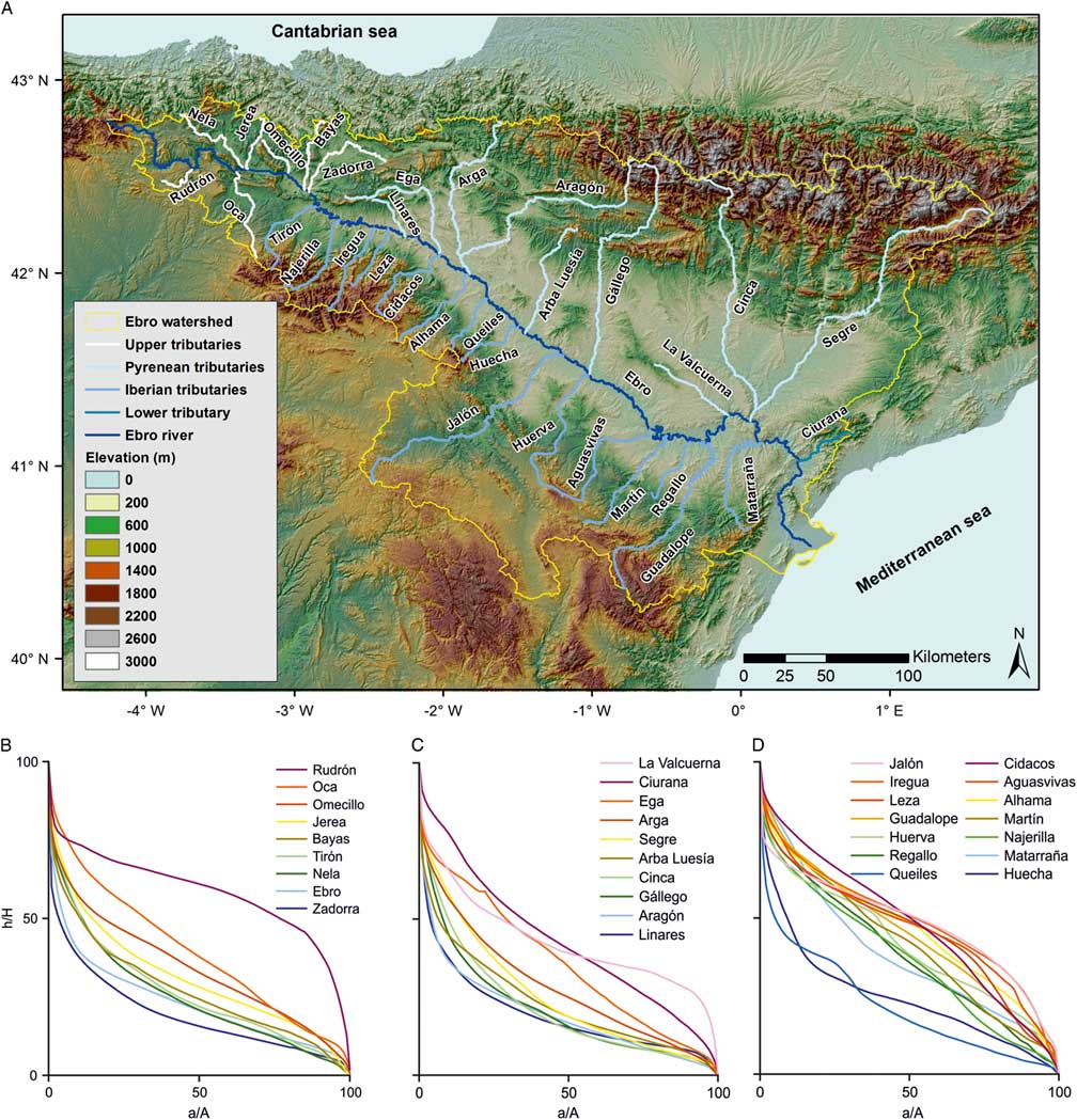
The Ebro catchment is one of the largest fluvial systems in Iberia (>85,000 km2). It is drained by the Ebro River, which runs eastward for 970 km from the northern Basque-Cantabrian Mountains to the Mediterranean Sea, where it forms the Ebro delta. It is bounded by the Basque-Cantabrian Mountains, the Pyrenees, the Iberian Range, and the Catalan Coastal Ranges (Fig. 1).
(colour online) (A) Geologic map of the Ebro catchment, showing the trunk river and its main tributaries. 1, Almazán basin; 2, Calatayud basin. (B) Longitudinal profile of the Ebro River; black arrows show the limits between the upper Ebro catchment (UEC), the Ebro foreland basin (EFB), and the lower Ebro catchment (LEC).
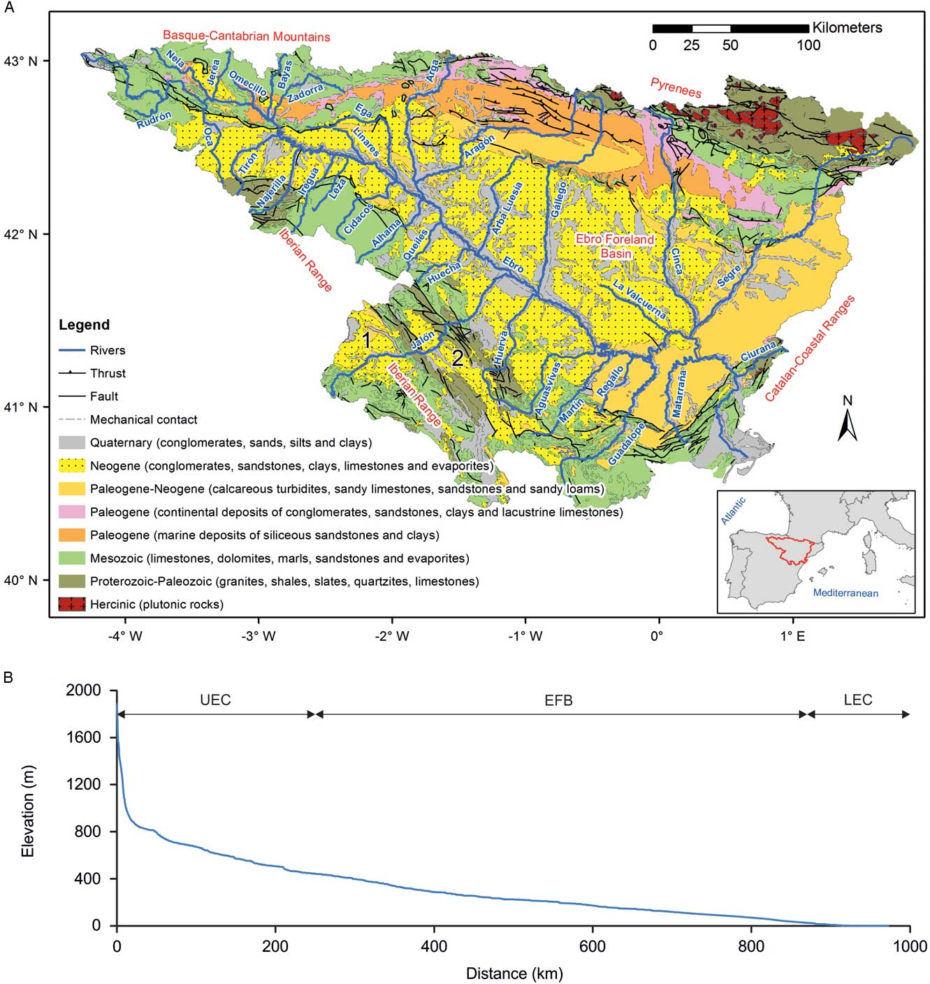
The Ebro foreland basin (EFB) encompasses the central area of the catchment. It resulted from the collision between the Iberian and European plates from the Late Cretaceous to the Early Miocene (Muñoz et al., Reference Muñoz, Arenas, González, Luzón, Pardo, Pérez and Villena2002). The geodynamic evolution of the basin was linked to the uplift and structural development of the surrounding reliefs during the alpine orogeny (Muñoz, Reference Muñoz1992).
The EFB is delimited to the north by the South Pyrenean Zone, north of the Southern Pyrenean Thrust (Barnolas and Pujalte, Reference Barnolas and Pujalte2004). This unit is composed of Mesozoic and Cenozoic marine and continental deposits detached from the Variscan basement through a thrust system (Sibuet et al., Reference Sibuet, Srivastava and Spakman2004) (Fig. 1). These thrust sheets are partly buried beneath Late Cretaceous to Early Miocene synorogenic sediments, deposited in piggyback basins. They are rooted in the Pyrenean Axial Zone, an antiformal stack of Palaeozoic and pre-Palaeozoic rocks (Mattauer, Reference Mattauer1990; Capote et al., Reference Capote, Muñoz, Simón, Liesa and Arlegui2002).
To the west, the upper Ebro catchment (UEC) is located in the southwestern sector of the Basque-Cantabrian Mountains, a synclinorium composed of Cretaceous to Paleogene marine and continental sedimentary rocks, mainly comprising limestones, siltstones, sandstones, and conglomerates (Feuillée and Rat, Reference Feuillée and Rat1971; Floquet, Reference Floquet1991; Pluchery, Reference Pluchery1995) (Fig. 1). The UEC was separated from the EFB, at least during the Tortonian (11.6–7.2 Ma) (Ramírez del Pozo, Reference Ramírez1973). Its base level was located behind the Western Pyrenean Thrust (the continuation of the Southern Pyrenean Thrust; Fig. 1). It connected with the EFB sometime during the Upper Miocene–Early Pliocene (Gonzalo Moreno, Reference Gonzalo Moreno1979).
To the south, the Iberian Range is an alpine, intraplate thrust belt, structurally defined by two northwest–southeast striking arches, which resulted from the inversion of Mesozoic extensional basins (van Wees et al., Reference van Wees, Arche, Beijdorff, Lopez-Gomez and Cloetingh1998; Salas et al., Reference Salas, Guimerà, Mas, Martín-Closas, Meléndez and Alonso2001; De Vicente et al., Reference De Vicente, Vegas, Muñoz-Martín, Van Wees, Casas-Sáinz, Sopeña and Sánchez-Moya2009) (Fig. 1). It consists of Permian and Mesozoic sedimentary rocks, lying unconformably over the Variscan basement. The Iberian Range is a dome-shaped relief, characterised by a high-standing but low surface. The uplift experienced by the Iberian Range is under debate. Some models have proposed that the uplift was generated by large-scale lithospheric folding (Cloetingh et al., Reference Cloetingh, Burov, Beekman, Andeweg, Andriessen, García-Castellanos, De Vicente and Vegas2002; De Vicente et al., 2009); a late-stage, compressive episode or erosional unloading (Casas-Sainz and De Vicente, Reference Casas-Sainz and De Vicente2009); or the possible action of a mantle upwelling (Boschi et al., Reference Boschi, Faccenna and Becker2010; Faccenna and Becker, Reference Faccenna and Becker2010). The Iberian Range also includes internal Cenozoic basins, some of which experienced endorheic drainage conditions until the end of Pliocene, when they were captured by the surrounding fluvial systems (Gutiérrez-Santolalla et al., Reference Gutiérrez-Santolalla, Gracia and Gutiérrez-Elorza1996; Gutiérrez et al., Reference Gutiérrez, Gutiérrez, Gracia, McCalpin, Lucha and Guerrero2008). The main examples are the Almazán, Calatayud, and Teruel basins (Anadón et al., Reference Anadón, Alcalá, Alonso-Zarza, Calvo, Ortí and Rosell2004) (Fig. 1).
To the east, the Catalan Coastal Ranges are a system of narrow mountain ranges and basins with a northeast–southwest orientation, subparallel to the Mediterranean coast (Fig. 1). The basin is in the front of an inverted, northeast–southwest oriented, Early Mesozoic extensional basin and is structurally dominated by basement materials involving steep up-thrusts that reactivated Mesozoic extensional faults (Lawton et al., Reference Lawton, Roca and Guimerà1999). The age of the compressive structures ranges from Middle Eocene to Late Oligocene (Christie-Blick and Biddle, Reference Christie-Blick and Biddle1985). Two lithologic domains are present: the southern sector, comprising Mesozoic carbonate rocks, and the northern sector, composed of Palaeozoic granites and metamorphic rocks (Sopeña et al., Reference Sopeña, Gutiérrez-Marco, Sánchez-Moya, Gómez, Mas, García and Lago2004).
The endorheic phase of the Ebro basin lasted at least until the Late Miocene. This period was dominated by fluvial systems rooted in the peripheral mountain ranges that fed various lacustrine environments in the central areas (Vera, Reference Vera2004). The synorogenic, endorheic sedimentation of the foreland basin is characterised by conglomerates passing laterally into sandstones, lutites, lacustrine limestones, and evaporites towards the depocentre (Riba et al., Reference Riba, Reguant and Villena1983). The opening of the Ebro basin caused a major change in the base level of the basin (Riba et al., Reference Riba, Reguant and Villena1983), triggering fluvial incision and the widespread erosion of the endorheic sedimentary infill (Gutiérrez Elorza et al., Reference Gutiérrez Elorza, García-Ruiz, Goy, Gracia, Gutierrez-Santolalla, Martí, Martín Serrano, Pérez-Gonzalez, Zazo and Aguirre2002).
Basin erosion and valley entrenchment led to the formation of fluvial terraces during the Quaternary. These terraces can be divided into two types (Julián, Reference Julián1996). The first type is composed of large alluvial plains linked to braided fluvial systems. These are the deposits preserved at the highest altitude, more than 180 m above the current riverbeds. They appear in the Iberian Range tributaries, Najerilla and Iregua (Julián, Reference Julián1996), and in the Pyrenean tributaries, Alcanadre, Noguera Ribagorzana, Cinca, and Gállego (Alberto et al., Reference Alberto, Gutiérrez, Ibáñez, Machín, Meléndez, Peña, Pocoví and Rodríguez1983). The second type corresponds to terrace staircases. These are described in the Ebro River (Soriano, Reference Soriano1990; Leránoz, Reference Leránoz1993; Julián, Reference Julián1996; Soria-Jáuregui et al., Reference Soria-Jáuregui, González-Amuchástegui, Mauz and Lang2016) and in most of its tributaries (Julián, Reference Julián1996; Peña-Monné and Sancho, Reference Peña-Monné and Sancho1988; Guerrero et al., Reference Guerrero, Gutiérrez and Lucha2008; Benito et al., Reference Benito, Sancho, Peña, Machado and Rhodes2010; Lewis et al., Reference Lewis, Sancho, McDonald, Peña-Monné, Pueyo, Rhodes, Calle and Soto2017). In some cases, the correlation of these terraces is complex because they are affected by neotectonic movements (Turú i Michels and Peña-Monné, Reference Turú i Michels and Peña-Monné2006) or by karstic subsidence processes (Benito et al., Reference Benito, Sancho, Peña, Machado and Rhodes2010; Luzón et al., Reference Luzón, Rodríguez-López, Pérez, Soriano, Gil and Pocoví2012; Gil et al., Reference Gil, Luzón, Soriano, Casado, Pérez, Yuste, Pueyo and Pocoví2013). The most complete terrace sequences are made up of a maximum of 12 levels in the Gállego River (Benito et al., Reference Benito, Sancho, Peña, Machado and Rhodes2010) and the Huerva River (Guerrero et al., Reference Guerrero, Gutiérrez and Lucha2008). The Ebro River has a maximum of 11 levels (Leránoz, Reference Leránoz1993).
The chronological study of terraces indicates that terrace formation extends from the early Pleistocene (1276 ± 104 ka) (Sancho et al., Reference Sancho, Calle, Peña-Monné, Duval, Oliva-Urcía, Pueyo, Benito and Moreno2016) to the Holocene (e.g., Soria-Jáuregui et al., Reference Soria-Jáuregui, González-Amuchástegui, Mauz and Lang2016). According to Stange et al. (Reference Stange, van Balen, Vandenberghe, Peña and Sancho2013), terrace formation seems to be related to the synchronous action of Quaternary climatic oscillations and tectonic uplift. Aggradation phases are linked to the delivery of large volumes of sediment, originating in the surrounding reliefs as a result of the expansion of glacial and/or periglacial conditions during the colder phases of the Quaternary (Whitfield et al., Reference Whitfield, Macklin, Brewer, Lang and Mauz2013; Lewis et al., Reference Lewis, Sancho, McDonald, Peña-Monné, Pueyo, Rhodes, Calle and Soto2017). The formation and preservation of entrenched, paired terraces across different basins required homogeneous uplift movements. Proposed uplift mechanisms include crustal shortening (Gallastegui et al., Reference Gallastegui, Pulgar and Gallart2002), erosional isostatic adjustments as a consequence of the opening of the Ebro basin (García-Castellanos and Larrasoaña, Reference García-Castellanos and Larrasoaña2015), and isostatic rebound as a consequence of crustal thickening (Casas-Sainz and De Vicente, Reference Casas-Sainz and De Vicente2009).
METHODOLOGY
Data preparation
The Ebro catchment has been analysed using a 90 m cell size, digital elevation model (SRTM Digital Elevation Database v4.1). This data set has vertical errors of less than 6 m for Eurasia (Jarvis et al., Reference Jarvis, Reuter, Nelson and Guevara2008). The required information was extracted using ArcGIS and SAGA GIS tools within QGIS.
The channel network was obtained from the Confederación Hidrográfica del Ebro and further corrected, with the drainage network being extracted from topographic data (Pastor-Martín et al., Reference Pastor-Martín, Antón and Fernández-González2017), to include the headwaters of streams, when appropriate (Fig. 2). The longitudinal profiles of the Ebro River and 32 of its tributaries were constructed and analysed (Fig. 3). Those profiles were corrected for the presence of dams using historic topographic maps published by the Instituto Geográfico Nacional (scale 1:50,000) and topographic maps produced for the dam construction sites of Quintana, Puentelarra, and El Cortijo provided by the Confederación Hidrográfica del Ebro (scale 1:2500). In the absence of the aforementioned topographic information, the effect of dams within the longitudinal profiles was removed by interpolation between the lowest and highest points, where the dam anomaly was present in the longitudinal profile.
(colour online) (A) Digital elevation model of the Ebro catchment displaying the main channel network. (B) Hypsometric curves for the Ebro River and its upper tributaries. (C) Hypsometric curves for the Pyrenean and lower tributaries. (D) Hypsometric curves for Iberian Range tributaries.

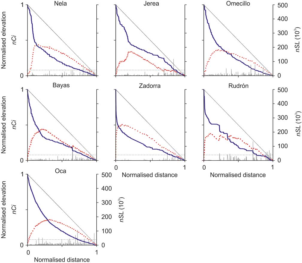
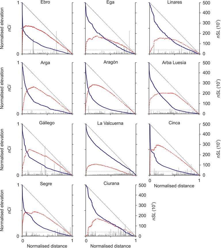
Normalised longitudinal profiles for the Ebro River and its tributaries. Thick red, dotted lines illustrate normalised concavity index (nCi) values, and grey lines indicate normalised stream gradient index (nSL) values along the profiles. Fine, black, dotted lines are reference lines that connect the divides with the river mouths. (3A) Normalised longitudinal profiles for the upper tributaries. (For interpretation of the references to colour in this figure legend, the reader is referred to the web version of this article.)
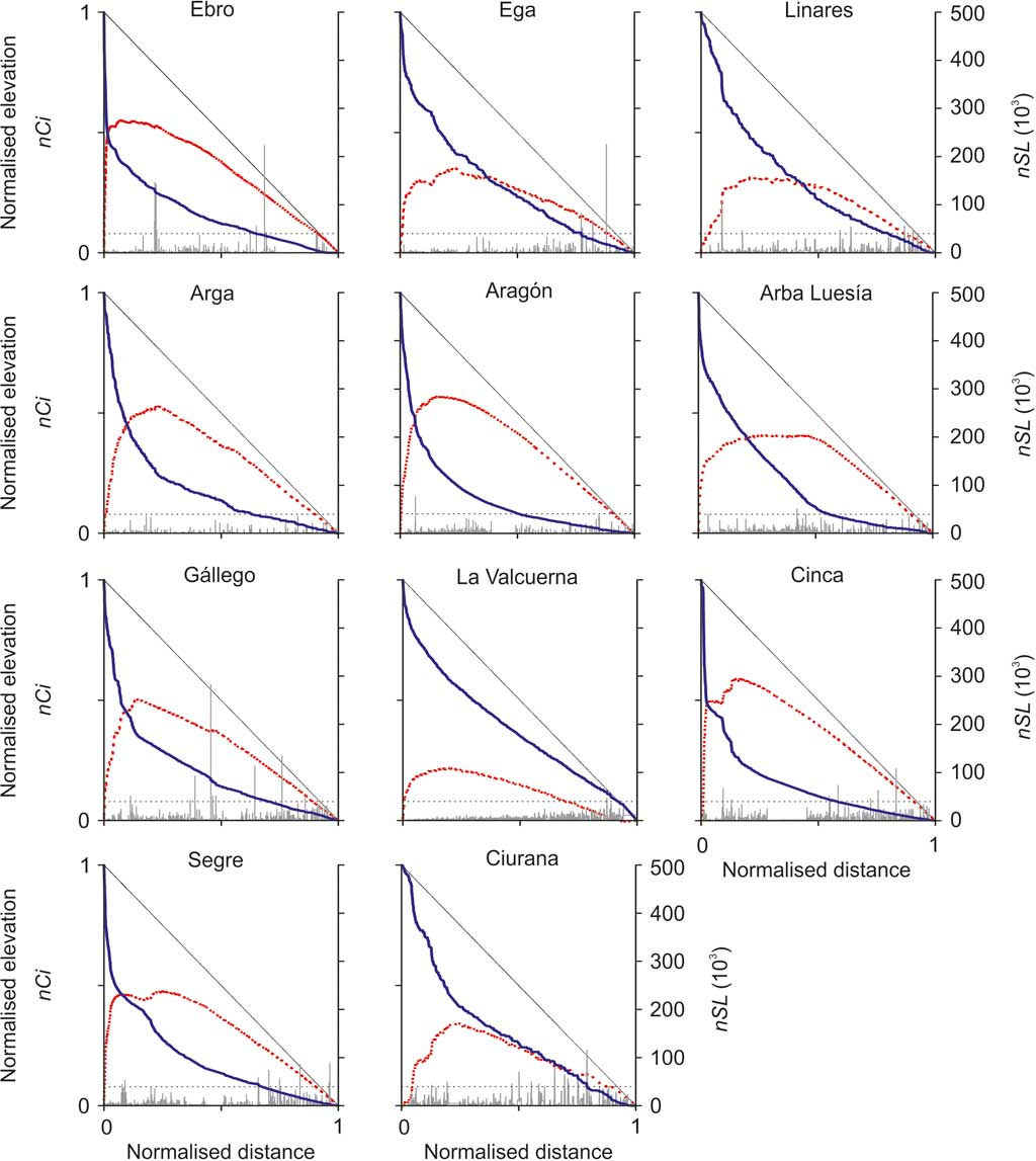
Normalised longitudinal profiles for the Ebro and the Pyrenean and lower tributaries. (For interpretation of the references to colour in this figure legend, the reader is referred to the web version of this article.)
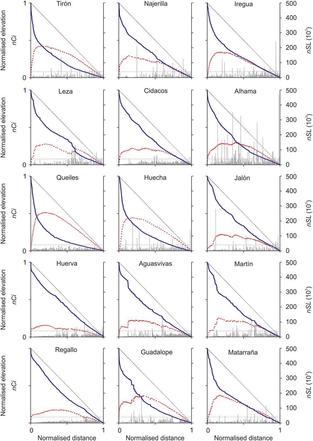
Normalised longitudinal profiles for the Iberian Range tributaries. (For interpretation of the references to colour in this figure legend, the reader is referred to the web version of this article.)
For each of the 33 streams, a number of topographic parameters were extracted from the digital elevation model, including stream length, contributing drainage area, headwater-confluence altitudinal difference, and the distance to the Mediterranean river mouth of the Ebro (Table 1). To enable analysis between rivers of different lengths and gradients, the stream profiles were normalised (Demoulin, Reference Demoulin1998) with regard to their height and to their length (Fig. 3). These normalised values were used to visually identify knickzones in the longitudinal profiles of the river and to calculate the normalised concavity index (nCi). Rough data were used to calculate the normalised stream gradient index (nSL).
Characteristics of the Ebro River and its tributaries and normalised concavity index (nCi), hypsometry integral (HI), and asymmetry factor (AF) values.

Normalised stream gradient index
The stream gradient index (SL) highlights changes in the topographic gradient along the streams’ longitudinal profiles (Hack, Reference Hack1973; Keller and Pinter, Reference Keller and Pinter2002). The SL tends to be high upstream, in sectors where bedrock has a high erosional resistance and in tectonically active areas (Hack, Reference Hack1973; Merritts and Vincent, Reference Merritts and Vincent1989; Brookfield, Reference Brookfield1998; Bishop et al., Reference Bishop, Hoey, Jansen and Artza2005; Pérez-Peña et al., Reference Pérez-Peña, Azor, Azañón and González-Lodeiro2009b; Antón et al., Reference Antón, De Vicente, Muñoz-Martín and Stokes2014). Thus, variations in the SL will indicate the presence of knickpoints/knickzones, highlighting potential tectonic activity and lithologies with contrasting resistance along the analysed longitudinal profiles.
For a segment of a given river course, the SL is calculated as follows:
 $$SL{\equals}\left( {dh\,/\,dl} \right)L,$$
where dh/dl is the gradient of a given segment, and L is the horizontal length from the midpoint of the segment to the catchment divide (Hack, Reference Hack1973).
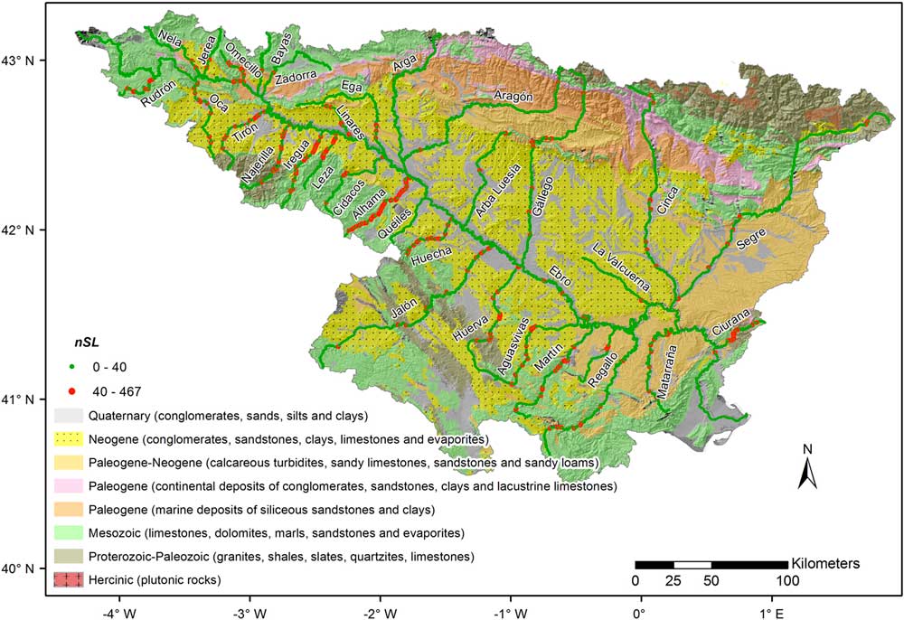
The SL is very sensitive to river length, making comparisons among rivers with significantly different sizes challenging. However, the use of a normalised profile for the SL calculation is not possible, as the channel slope would then need to be modified. To avoid this issue, a normalised index was performed. The nSL is the result of the SL values of the stream, normalised by its total length. The normalised results were then multiplied by a factor of 103 to obtain comprehensive numbers (Fig. 3). The nSL values were mapped to improve the visualisation of their spatial distribution, as well as to check the location of anomalously high nSL values along the catchment and their potential relationship with geologic and/or structural features (Fig. 4).
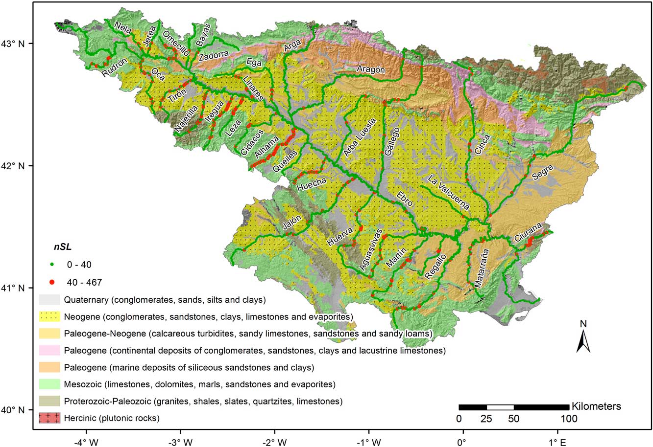
(colour online) Geologic map of the Ebro catchment showing the spatial distribution of normalised stream gradient index (nSL) values across the channel network.
Normalised concavity index
River channels in a steady state have a concave-up longitudinal profile (Hack, Reference Hack1957, Reference Hack1973; Flint, Reference Flint1974). Variations from that concave shape relate to changes in factors governing the evolution of a fluvial system such as tectonic activity or lithologic, environmental, or base-level changes (Snyder et al., Reference Snyder, Whipple, Tucker and Merritts2000; Zaprowski et al., Reference Zaprowski, Pazzaglia and Evenson2005; Demoulin, Reference Demoulin2011; Burbank and Anderson, Reference Burbank and Anderson2012). The endorheic–exorheic transition experienced by the Ebro catchment implied that rivers had to adjust their profiles to the Mediterranean base level. Some rivers, like the Duero River, developed convex sectors within their profiles after experiencing a base-level fall (Antón et al., Reference Antón, Rodés, De Vicente, Pallàs, Garcia-Castellanos, Stuart, Braucher and Bourlès2012). Such variations in a longitudinal profile can be revealed by the concavity index (Ci) because it enables the quantification of the curvature of a longitudinal profile (Demoulin, Reference Demoulin1998; Phillips and Lutz, Reference Phillips and Lutz2008; Antón et al., Reference Antón, De Vicente, Muñoz-Martín and Stokes2014). In order to make the results from the Ebro River and 32 of its tributaries comparable, normalised longitudinal profiles were used. By drawing a straight line connecting the highest point within a graph of the profile (headwater) with the lowest (river mouth/confluence), a triangle is created. In a normalised longitudinal profile, the area of this triangle is 0.5 units. The area under the normalised longitudinal profile is subtracted from the triangle area and divided by 0.5 units to normalise the results. The resulting nCi values vary from −1 (very convex forms) to +1 (very concave forms) (Table 1). A value of 0 corresponds to a linear longitudinal profile.
The nCi was also calculated for every point within the longitudinal profiles as the difference between the height of the triangle and the normalised height over each point of the profile. Plotting nCi values for every point along a given profile allows investigation of the concavity of the different segments forming the entire profile. The calculation of individual values of nCi identifies relatively limited convex sectors that can be overlooked by the general concavity index. It also provides a better picture of the morphological evolution of the longitudinal profile on a map (Figs. 3 and 5). A theoretical graded profile, the initial points of the profile are close to the straight line connecting the highest and the lowest points of the profile, so nCi values for those points are expected to be close to zero. Concavity values get closer to 1 in the middle reaches of the stream as its points are further away from the drawn straight line. Near the downstream limit (mouth or confluence), profile points get closer to the straight line again, and calculated nCi values approach zero (Fig. 5B). Thus, anomalies should be identified in areas where deviations from that pattern occur.
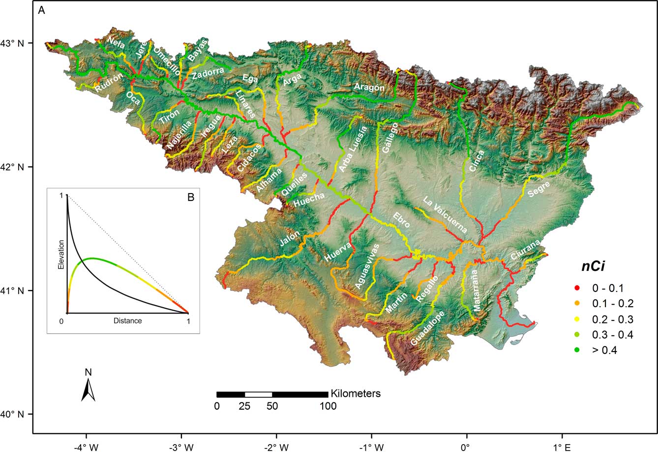
(colour online) (A) Digital elevation model of the Ebro catchment showing the spatial distribution of normalised concavity index (nCi) values across the channel network. (B) Theoretical graded longitudinal profile (black) and the evolution of the nCi values along the profile (coloured).
Hypsometry
Hypsometry is the relationship between area and altitude within a catchment (Strahler, Reference Strahler1952). We investigated the hypsometry of the Ebro catchment and its subcatchments by calculating the hypsometric curve (HC) and the hypsometric integral (HI) (Table 1, Fig. 2). The HC reflects the proportional area of the catchment above or below a certain altitude, whereas the HI represents the area under the HC (Keller and Pinter, Reference Keller and Pinter2002).
The HI was calculated using the following expression:
 $$HI{\equals}\left( {H_{{{\rm mean}}} -H_{{{\rm min}}} } \right)\,/\,\left( {H_{{{\rm max}}} -H_{{{\rm min}}} } \right),$$
where H mean represents the mean elevation of the catchment above sea level, H min is the minimum elevation, and H max is the maximum elevation of the catchment. HI values vary between 0 and 1.
The shape of the HC and HI values were initially applied to infer basin maturity (Strahler, Reference Strahler1952). Convex shapes with correspondingly high HI values were related to “young” catchments because relatively large portions of uneroded topography were still preserved under the curve. On the contrary, concave curves with low hypsometric integrals were interpreted as mature catchments where most of the watershed topography was already eroded. Sinuous shapes of the HC with intermediate HI values characterised some of the intermediate, erosional stages. A number of investigations carried out since the initial article by Strahler (Reference Strahler1952) have highlighted that hypsometry is also affected by a number of factors such as climate, tectonics, or lithology (Ohmori, Reference Ohmori1993; Willgoose and Hancock, Reference Willgoose and Hancock1998; Walcott and Summerfield, Reference Walcott and Summerfield2008; Pérez-Peña et al., Reference Pérez-Peña, Azor, Azañón and Keller2010; Marchi et al., Reference Marchi, Cavalli and Trevisani2014). Lifton and Chase (Reference Lifton and Chase1992) concluded that tectonics influence hypsometry at large scales, whereas lithologic influences were dominant at local scales. Also, because hypsometry is directly related to relief and its dissection, it enables exploration of the importance of fluvial versus hillslope processes in a given basin (Hurtrez et al., Reference Hurtrez, Sol and Lucazeau1999). In the Ebro basin, this hypsometrical analysis will provide information on the maturity of the exorheic catchment and on the extent of the postopening dissection. The combination of convex-up curves and high HI responds to poorly incised areas where geomorphological activity is controlled by hillslope processes or uplifted low reliefs with minor fluvial erosion; concave-up curves and low HI are related to landscapes with a high degree of dissection, where fluvial erosion is dominant (Hurtrez et al., Reference Hurtrez, Sol and Lucazeau1999; Keller and Pinter, Reference Keller and Pinter2002).
Asymmetry factor
The geometry of a catchment may be strongly influenced by tectonics and/or lithologic conditions. One way to evaluate such an impact is to study the basin asymmetry. The asymmetry factor (AF) may infer the presence of tilting in a fluvial basin. It is calculated as follows (Keller and Pinter, Reference Keller and Pinter2002):
 $$AF{\equals}100{\rm }\left( {A_{r} \,/\,A_{t} } \right),$$
where A r is the area of the fluvial basin to the right of the trunk channel, and A t is the total area of the catchment.
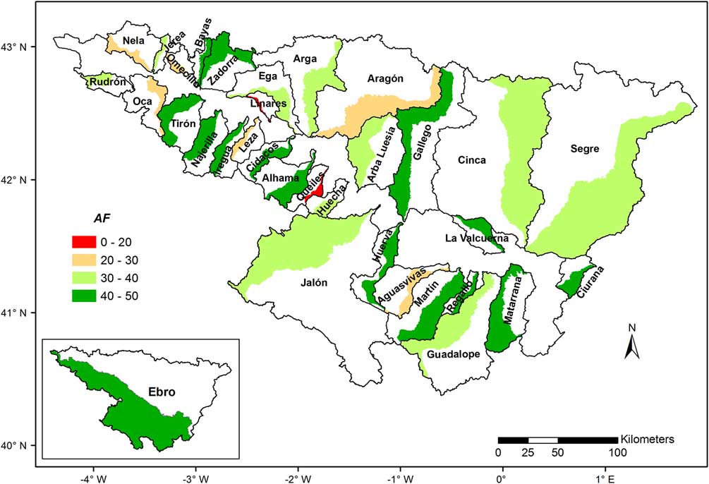
This index helps us to elucidate the existence of regional uplift versus differential uplift among the different subbasins and indicates whether block tilting is involved. Figure 6 shows the AF values for the Ebro catchment and the catchments of the studied tributaries.
(colour online) Schematic map of subcatchments showing the asymmetry factor (AF) values. Only the smallest halves of the catchments are depicted, as they show the side towards which the river seems to be migrating. Bottom left, AF value for the entire Ebro catchment.

Mountain front sinuosity
Bull and McFadden (Reference Bull and McFadden1977) defined mountain front sinuosity (S mf ) as follows:
 $$S_{{mf}} {\equals}L_{{mf}} \,/\,L_{S} ,$$
where L mf is the length of the mountain front along the foot of the mountain-piedmont junction, and L s is the straight-line length of the mountain front. This index reflects the balance between tectonic and erosional processes along mountain fronts (Bull and McFadden, Reference Bull and McFadden1977; Keller and Pinter, Reference Keller and Pinter2002). Mountain fronts, where uplift is the dominant mechanism, are characterised by sublinear geometries. However, erosional processes will tend to produce sinuous geometries. Values of S mf below 1.4 indicate tectonically active fronts, whereas higher values indicate tectonically quiescent areas where erosion is the main process (Rockwell et al., Reference Rockwell, Keller and Johnson1984; Keller, Reference Keller1986). The mountain fronts bounding the Ebro basin were measured in discrete segments according to the criteria proposed by Wells et al. (Reference Wells, Bullard, Menges, Drake, Karas, Kelson, Ritter and Wesling1988) (Fig. 7). Different S mf values in the surrounding mountain fronts might indicate the existence of contrasting uplift rates among the reliefs (Pérez-Peña et al., Reference Pérez-Peña, Azor, Azañón and Keller2010).
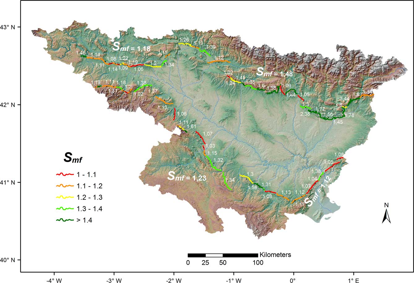
(colour online) Map showing the segments used for mountain front sinuosity (S mf ) calculation and their individual values (Table 2). Also, the mean values for each region are presented in larger, bold letters.
RESULTS
Longitudinal profiles
The visual investigation of the longitudinal profiles reveals that most of the Upper Ebro streams and the Pyrenean tributaries, as well as the Ebro and Ciurana Rivers, show a generally concave shape (Fig. 3A and B). An exception to this is the Valcuerna River, which presents a sublinear shape. Within the concave longitudinal profiles, limited convex segments are present in some cases, like in the Segre and Jerea Rivers, among others (Fig. 3A and B). Another group, comprising the Iberian Range tributaries, is formed by those profiles that are sublinear or irregular in shape (Fig. 3C).
Normalised stream gradient index
The nSL values for each point along the longitudinal profiles are shown in Figures 3 and 4. Values range from 0.00 to 466.56, and these were grouped into two classes: 0–40 and 40–467. The visual investigation of the longitudinal profiles revealed that the most relevant gradient changes were marked by nSL values of 40 or higher (Fig. 3). The statistical analysis of the data showed that nSL values of 40 or higher represent 0.5% of the total values. Also, the threshold coincides with about five times the standard deviation (Font et al., Reference Font, Amorese and Lagarde2010; Viveen et al., Reference Viveen, van Balen, Schoorl, Veldkamp, Temme and Vidal-Romaní2012). Hence, for the purposes of this study, values greater than 40 are representing both geomorphological and statistical anomalies. The distribution of those anomalies along the Ebro catchment is heterogeneous. The northwestern Iberian Range tributaries display the highest concentration, whereas the rest of the analysed courses present a lower volume of nSL high values (Fig. 4). In the UEC, the Jerea and Rudrón Rivers exhibit numerous nSL spikes, in relation to their irregular longitudinal profiles (Fig. 3A). Pyrenean tributaries present a comparatively smaller number of anomalies that are distributed in the uppermost reaches, at the crossing of the South Pyrenean Thrust and along the course of the foreland basin (Fig. 4). It has already been highlighted that among the Iberian Range tributaries, the northwestern rivers are those that have higher nSL values (Fig. 3C). The Alhama River stands out, with the presence of numerous anomalies throughout its entire course. The rest of the rivers of the Iberian Range, especially those in the central sector, show fewer anomalies because they have a lower general gradient (Fig. 4). A noteworthy feature of the distribution of gradient anomalies is that rivers draining the foreland basin exhibit a relatively high concentration of nSL peaks along the stretches that flow over Neogene sediments, especially (but not only) the Iberian Range tributaries.
Normalised concavity index
The nCi has been used to highlight deviations of a longitudinal river profile from its theoretical, steady-state, concave-up shape. First, we calculated the nCi index for whole profiles (Table 1). The general concavity values are all positive because the analysed profiles are defined as concave or sublinear. There is no entirely convex profile. The nCi values range between 0.20 and 0.70, with a mean value of 0.45. The longest and largest rivers tend to display the highest concavity values, with the notable exception of the Jalón River (nCi=0.28). Higher values are found in the Pyrenean tributaries, with the exception of the La Valcuerna River (a tributary approximately 175 km upstream from the mouth of the Ebro River), which exhibits a sublinear profile (Fig. 3B). The central and southeastern rivers flowing down the Iberian Range are the less concave courses (Table 1).
We also computed the nCi values for each point along the longitudinal profiles in order to identify possible convex or linear sectors within a profile (Figs. 3 and 5). These individual nCi values range from a maximum of 0.6 (in the most concave sectors) to a minimum of 0.0 in the headwaters and river mouths (Fig. 3B and C). Watercourses with major convex sectors within their profiles include the Rudrón, Leza, Cidacos, Jalón, Huerva, Jerea, Bayas, and Segre Rivers. These convex reaches are identifiable by a sudden rise of values within a given segment otherwise characterised by lower nCi (Fig. 5). The overall concavity of a profile can be investigated using the map of the individual nCi values (Fig. 5). The most linear longitudinal profiles are easily identifiable in Figure 5 because they do not display dark green values. These include the Najerilla, Leza, Cidacos, Alhama, Jalón, Huerva, Aguasvivas, Martín, Regallo, and La Valcuerna Rivers.
Hypsometry
Calculated hypsometric curves are shown in Figure 2. The Ebro River, its upper tributaries, and the Pyrenean tributaries are characterised by the concave-up shapes of the hypsometric curves, suggesting a high degree of dissection (Fig. 2B and C). The Rudrón River is the only stream among the analysed rivers that is characterised by a pronounced convex shape of the hypsometric curve (Fig. 2B). This upper tributary flows over the high plateau of La Lora, which is reflected in the amount of the catchment area situated at high altitudes (Fig. 2A). La Valcuerna River also stands out within the Pyrenean tributaries because of the convex segment of the lower end of the hypsometric curve (Fig. 2C).
The hypsometric curves for the Iberian tributaries are characterised by S-shaped curves, which indicates that a great part of their catchment relief is at a relatively high elevation (Fig. 2D). Also, the sharp decrease in area volume towards the river mouths might indicate base-lowering processes. Only the Queiles and Huecha Rivers display concave-up hypsometric curves. These are two of the shortest and steepest rivers in this study. These rivers quickly abandon the harder reliefs of the Iberian Range and enter the softer EFB. This means that a significant percentage of their catchment area is located at relatively low altitudes (Fig. 2A and D).
HI values range between 0.58 (Rudrón River) and 0.19 (Zadorra River) (Table 1). Despite the fact that both extreme values are found in the UEC, there is a clear distinction between the Pyrenean and upper tributaries (that exhibit a lower mean HI value of 0.28) and the Iberian Range tributaries (that show a higher HI mean value of 0.40; Table 1, Fig. 8B).
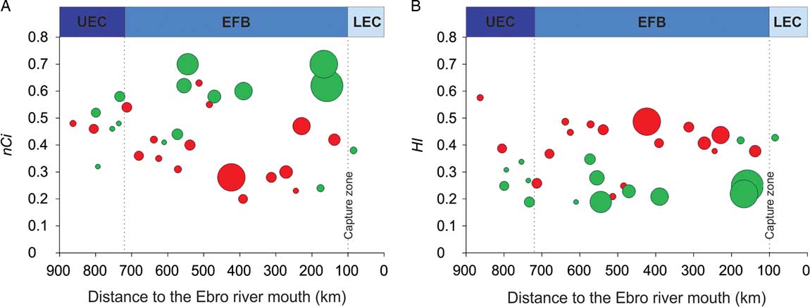
(A) Normalised concavity index (nCi) versus distance to the Ebro outlet. (B) The hypsometric integral (HI) versus distance to the Ebro outlet. The size of the circles is in relation to the catchment area. Green circles indicate Ebro northern tributaries. Red circles indicate Ebro southern tributaries. Green circles within the EFB are the Pyrenean tributaries, whereas the red circles within the EFB are the Iberian Range tributaries. EFB, Ebro foreland basin; LEC, lower Ebro catchment; UEC, upper Ebro catchment. (For interpretation of the references to colour in this figure legend, the reader is referred to the web version of this article.)
Asymmetry factor
The AF values for the Ebro River and its 32 tributaries range from 13 to 73 (Table 1). To facilitate the interpretation of the potential migration of the streams, the smallest half of each basin was the one coloured in the map, as it illustrates the side towards which the trunk river would be migrating (Fig. 6). Watersheds were classified according to their AF values, where AF <20 identifies strongly asymmetric catchments; AF=20–30, moderately asymmetric catchments; AF=30–40, gently asymmetric catchments; and AF=40–50, symmetric catchments (Table 1, Fig. 6). Two upper watersheds are defined as being symmetric, two gently asymmetric, and three moderately asymmetric. Pyrenean and Iberian Range catchments (approximately 78% and 80% of them, respectively) are defined as gently asymmetric and symmetric. Also, the Ebro catchment, as a whole, is considered to be symmetric (AF=41) (Fig. 6). One of the main results of the asymmetry factor is that despite the fact that uplift movements may be affecting several areas across the Ebro catchment, there is a lack of significantly asymmetric basins. This may rule out block tilting as a relevant process affecting the basin.
Mountain front sinuosity
A total of 66 segments were measured along the mountain fronts surrounding the EFB (Fig. 7). Calculated values of S mf are shown in Table 2. The Pyrenean front was measured along 23 segments, with the highest value of 3.44, the lowest S mf value of 1.03, and a mean value of 1.48. Values of front sinuosity for the Iberian Range were obtained for 20 segments and ranged from 1.02 to 1.61, yielding an average value of 1.23. Mountain front sinuosity in the Basque-Cantabrian Mountains was measured along 17 segments and ranged from 1.05 to 1.41; the mean value of S mf for this region is 1.17. The values of S mf for the Catalan Coastal Ranges ranged from 1.04 to 1.38 along 6 segments, which yielded an average value of 1.12.
Mountain front sinuosity (S mf ) values for the individual mountain front segments and their regional mean values. L mf , length of the mountain front along the foot of the mountain-piedmont junction; L s, straight-line length of the mountain front.
DISCUSSION
Given that the EFB has been exposed to the Mediterranean base-level for a prolonged time (Babault et al., Reference Babault, Loget, Van Den Driessche, Castelltort, Bonnet and Davy2006; Arche et al., Reference Arche, Evans and Clavell2010; García-Castellanos and Larrasoaña, Reference García-Castellanos and Larrasoaña2015), it is likely that the emptying of the endorheic infill has reached a significant stage of its development (Antón et al., Reference Antón, Muñoz-Martín, De Vicente and Finnegan2017). The results obtained provide evidence that the Ebro catchment as a whole presents a concave-up shape in its hypsometric curve, a low HI, and a low AF value (Table 1, Figs. 2B and 6). The longitudinal profile of the Ebro River is characterised by an overall concave form, a lack of knickzones, low nSL values, and high nCi (Figs. 1B and 3B). A close inspection of the Ebro River shows a minor presence of gradient anomalies, related to structural and lithologic boundaries, as well as meander cutoffs (Figs. 3B and 4). These morphometric characteristics are typical of a mature, moderately to highly erosional area where fluvial processes are dominant, suggesting that the Ebro catchment has reached an advanced phase of adjustment after the opening of the basin to the Mediterranean Sea. This is in agreement with morphological evidence preserved across the EFB. The central areas of the EFB are made up of rocks that are less resistant to erosion (e.g., evaporites and clays; Fig. 1), so the headward erosion and incision processes might have been particularly effective in this setting. In that sense, one of the youngest endorheic sequences preserved in the central area is located at an elevation of 812 m above sea level (asl) at San Caprasio (Pérez-Rivarés et al., Reference Pérez-Rivarés, Garcés, Arenas and Pardo2002), while the currently active channel of the Ebro River in the surrounding area is located at approximately 170 m asl. Therefore, a minimum denudation of 642 m has taken place in the central foreland basin since the start of the exorheism (Lewis et al., Reference Lewis, Sancho, McDonald, Peña-Monné, Pueyo, Rhodes, Calle and Soto2017).
This erosional tendency is also recorded within the fluvial landscape. The formation of terrace sequences has been widespread. The highest and oldest remnants are associated with low-gradient river courses that formed wide alluvial plains, whereas the younger levels form terraced staircases in progressively entrenched river valleys (Alberto et al., Reference Alberto, Gutiérrez, Ibáñez, Machín, Meléndez, Peña, Pocoví and Rodríguez1983; Peña-Monné and Sancho, Reference Peña-Monné and Sancho1988; Julián, Reference Julián1996). This morphological evolution requires a change from lateral erosional or aggradational dynamics towards vertical incision. This dynamic shift is evident along the longitudinal profiles of the terraces of several tributaries of the Ebro River, which reveal a marked vertical separation between adjacent terraces (Guerrero et al., Reference Guerrero, Gutiérrez and Lucha2008; Sancho et al., Reference Sancho, Peña-Monné, Calle, Lewis, McDonald, Pueyo, Gosse and Soto2012; Stange et al., Reference Stange, van Balen, Vandenberghe, Peña and Sancho2013; Lewis et al., Reference Lewis, Sancho, McDonald, Peña-Monné, Pueyo, Rhodes, Calle and Soto2017). In that regard, terraced staircases are a useful tool for calculating fluvial incision rates (Burbank and Anderson, Reference Burbank and Anderson2012). Available data for the Ebro drainage system vary from a minimum of 0.12 m/ka for the last 1.28 Ma (Sancho et al., Reference Sancho, Calle, Peña-Monné, Duval, Oliva-Urcía, Pueyo, Benito and Moreno2016) to a maximum of 0.47 m/ka for the middle and late Pleistocene for the middle reaches of the Pyrenean tributaries (Lewis et al., Reference Lewis, Sancho, McDonald, Peña-Monné, Pueyo, Rhodes, Calle and Soto2017). Based on calcareous tufa ages, maximum incision rates of 0.6 m/ka have been reported for the Iberian Range tributaries during the late Pleistocene (Scotti et al., Reference Scotti, Molin, Faccena, Soligo and Casas-Sainz2014).
Behind the general evolutionary trend of the Ebro catchment, our results indicate that there is differential behaviour across the basin. The Ciurana River, which drains the Catalan Coastal Ranges, is the closest tributary to the Ebro river mouth (<100 km). It is experiencing an adjustment process, as shown by its relatively linear HC, comparatively high HI value, low nCi (Figs. 2C and 7), and numerous knickpoints in the middle and lower reaches (Figs. 2 and 4). The Ciurana River should have attained a more or less steady state long ago given its location relatively close to the Mediterranean base level. However, this river course flows through narrow and deep valleys, suggesting that the incision processes are still ongoing. It has been proposed that the Catalan Coastal Ranges might have been affected by the Neogene extension of the western Mediterranean margin (Gunnell et al., Reference Gunnell, Zeyen and Calvet2008). In fact, Quaternary tectonic activity has been reported in the major faults of the ranges (Perea et al., Reference Perea, Masana and Santanach2012), and the sectors with the steepest profiles in the Ciurana River are located at fault crossings (see Fig. 1). Also, such tectonic activity seems to be in agreement with the low mean S mf value (1.12) of the mountain front of the Catalan Coastal Ranges; this is typical of active mountain fronts.
However, one of the main features identified in our results is the contrasting morphometric characteristics between the northern and southern tributaries, specifically between the Pyrenean and Iberian Range tributaries of the Ebro River. Figure 8 represents concavity and hypsometric integral values of the tributaries in relation to their distance from the Ebro outlet and their catchment area. In both charts, the distribution displays a clear difference between the north and the south. Neither group of tributaries show distinct trends between concavity or hypsometry and basin size and/or their distance from the capture zone or river outlet. In the case of the Pyrenean tributaries, the combination of both high nCi and low HI and their well-graded, longitudinal profiles suggests that the postopening incision penetrated both the large and the small basins across the entire Ebro catchment. This indicates a prolonged and intense period of erosion. This is also the case for the upper drainage network, located the farthest away from the capture zone. The upper tributaries generally display well-graded, longitudinal profiles with low nSL and high nCi values (Table 1, Fig. 3A), concave HCs, and relatively low HI values (Table 1, Fig. 2B). These geomorphic features are typical of deeply dissected basins. The exceptions to this are the Jerea, Rudrón and Oca tributaries (rivers still in a transient state). Also, there is no clear evidence of the opening of the upper Ebro towards the foreland basin, probably because of the relatively soft Cenozoic sedimentary rocks (sandstones, clays, and lacustrine limestones) to the rear of the Western Pyrenean Thrust.
The most relevant anomalies within the northern tributaries are present in the Pyrenean rivers. The middle and lower reaches of these rivers are relatively well “graded” to their current base level; however, the upper reaches present various convex reaches (Figs. 3B and 5). The lower and middle reaches drain the relatively soft rocks of the foreland basin, whereas the upper reaches are located within the Pyrenees, a structurally complex and lithologically harder relief, especially the igneous materials present in the core area of this cordillera (Fig. 1). Stange et al. (Reference Stange, van Balen, Vandenberghe, Peña and Sancho2013) described two knickpoints in the upper reaches of the Segre River, which are also identified in this study (Fig. 3B); these delayed the profile adjustment of the upper reaches. This anomaly is also present in the Cinca, Gallego, and Aragon Rivers. They can be interpreted as the effect of hard rocks on knickpoint migration (Figs. 3B and 4).
The morphometric indices for the Iberian Range tributaries are characterised by S-shaped HCs and high HI values (Table 1, Fig. 2D), which suggest these catchments are in a transient state further away from the steady state than the rest of the Ebro subcatchments. This “delayed” response is also seen in the longitudinal profiles of the central and southeastern Iberian Range tributaries, which display sublinear profiles and lower channel gradients. The most significant examples are the Huerva and Regallo Rivers, in which all nCi values lie below 0.2, showing that these rivers are far from the steady state, the values probably being a response to uplift movements (Table 1, Figs. 3C and 5). Based on geologic and geomorphological evidence, it can be inferred that the Iberian Range is affected by uplift movements that started during the Late Pliocene and have been active during the Quaternary, as recorded in the intramontane depressions of the inner Iberian Range (Simón, Reference Simón1983; Gutiérrez et al., Reference Gutiérrez, Gutiérrez, Gracia, McCalpin, Lucha and Guerrero2008; Casas-Sainz and De Vicente, Reference Casas-Sainz and De Vicente2009; Scotti et al., Reference Scotti, Molin, Faccena, Soligo and Casas-Sainz2014) (Figs. 3C and 5). Northwestern Iberian Range streams are characterised by a greater steepness and relatively more concave profiles (Figs. 3 and 4). In fact, these are the steepest rivers in the basin and might also be affected by neotectonic movements (Pérez-Lorente, Reference Pérez-Lorente1979, Reference Pérez-Lorente1983; Caro-Calatayud et al., Reference Caro-Calatayud, Pereda-Olasolo, Pérez-Gómez and Pérez-Lorente1989). Another difference among the longitudinal profiles of Iberian Range rivers is that the central and southeastern tributaries, especially the Jalón, Huerva, Aguasvivas, Martin, and Regallo Rivers, present lithologically controlled knickpoints that separate sections of contrasting concavity in the upper reaches (Figs. 3C and 4). These are related to the presence of intramontane Cenozoic basins in their headwaters, like the Calatayud and Almazán basins (Fig. 1). Endorheic conditions developed in these basins during the Cenozoic period. That resulted in a progressive filling in fluvial and lacustrine environments (Ortí and Rosell, Reference Ortí and Rosell2000). Subsequently, these basins were captured by the surrounding drainage network that, in the case of the Ebro tributaries, was driven by the upward erosion generated by the opening of the Ebro basin to the Mediterranean Sea (Gutiérrez et al., Reference Gutiérrez, Gutiérrez, Gracia, McCalpin, Lucha and Guerrero2008). Some of these captures are interpreted as being recent, like the capture of the Calatayud graben by the Huerva River that took place in the upper Pleistocene (Gutiérrez et al., Reference Gutiérrez, Gutiérrez, Gracia, McCalpin, Lucha and Guerrero2008). According to Giachetta et al. (Reference Giachetta, Molin, Scotti and Faccenna2015), the Iberian Range topography has experienced regional uplift since ca. 3 Ma with rates between 0.25 and 0.55 mm/yr. In response to this uplift, rivers have incised at an average long-term incision rate of approximately 0.22 mm/yr and have progressively captured drainage areas from the Iberian Range interior. Thus, the headwaters of these Iberian tributaries reflect the drainage networks whose base level was located inside those intramontane basins before being captured. This is also reflected in the concave-up shape of the upstream segments of the hypsometric curves and longitudinal profiles of these rivers (Figs. 2 and 3C). This suggests that these rivers are more developed in the upper reaches where they mirror the drainage network of the precapture landscape. The most obvious example is the Jalón River, whose longitudinal profile (Fig. 3C) displays three main lithologically controlled knickpoints that refer to the capture of the upper drainage network of the Almazán basin, the capture of the Almazán basin itself, and the capture of the Calatayud basin (Figs. 1A and 4). The same situation can be inferred for the Aguasvivas River, where the entrance to the Calatayud basin is identified in the profile by an abrupt knickpoint that separates a graded upper sector from the middle reaches (Figs. 3C and 4). Likewise, the profiles of the Huerva and Martin Rivers also display such anomalies (Fig. 3C). Given that the capture of these internal Cenozoic basins took place well after the setting of the exorheic conditions in the Ebro basin and the morphometric characteristics of the upper reaches of these rivers, we conclude that the upper sectors of these catchments graded to a base level different from the current one and that they are still adjusting to the Mediterranean base level. Similar morphologies are described in other captured basins where the transient response is still preserved (Antón et al. Reference Antón, Rodés, De Vicente, Pallàs, Garcia-Castellanos, Stuart, Braucher and Bourlès2012, Reference Antón, Muñoz-Martín and De Vicente2018; Martins et al., Reference Martins, Cabral, Cunha, Stokes, Borges, Caldeira and Cardoso Martins2017).
Nonetheless, our results suggest that, overall, the Ebro basin has reached an advanced phase of adjustment following the opening of the basin to the Mediterranean Sea. The landscape response involved the excavation of the endorheic fill by erosional processes migrating upstream and the development of graded longitudinal profiles along the basin. The adjustments of the drainage network in the upstream reaches also resulted in further drainage captures of the intramontane Cenozoic basins of the Iberian Range. A similar landscape response of the continental basins to base-level lowering has been observed in northeastern Tibet (Harkins et al., Reference Harkins, Kirby, Heimsath, Robinson and Reiser2007), the Sichuan basin (Richardson et al., Reference Richardson, Densmore, Seward, Fowler, Wipf, Ellis, Yong and Zhang2008), the Colorado River (House et al., Reference House, Pearthree and Perkins2008), the Sorbas basin in Spain (Harvey et al., Reference Harvey, Whitfield, Stokes and Mather2014), and the Duero basin in Iberia (Antón et al., Reference Antón, Rodés, De Vicente, Pallàs, Garcia-Castellanos, Stuart, Braucher and Bourlès2012). However, the degree of landscape dissection and the morphology of the longitudinal profiles would strongly depend on the evolutionary stage of the basin, in relation to the new base-level conditions (Antón et al., Reference Antón, Muñoz-Martín, De Vicente and Finnegan2017). This is clearly observed when comparing the Ebro and its neighbour, the Duero basin (Antón et al., Reference Antón, De Vicente, Muñoz-Martín and Stokes2014, Reference Antón, Muñoz-Martín and De Vicente2018). Both basins have a common history, at least until the late Neogene (Calvo et al., Reference Calvo, Daams, Morales and Lopez Martinez1993), and were subsequently captured. However, in the Duero basin there is a major knickzone in the middle reach where incision is very active and erosion has not yet dismantled the former Cenozoic basin. Regional morphometric analysis allows a quantitative analysis and comparison of how much a basin has attained a steady state under certain conditions and how much of the ancient landscape is preserved. In the Ebro basin, our results seem to indicate that the basin opening occurred before the Duero basin.
Additionally, the effects of processes such as drainage capture and differential tectonics can be inferred at a large scale. In the Pyrenean tributaries, Stange et al. (Reference Stange, van Balen, Vandenberghe, Peña and Sancho2013) hypothesised that the entrenchment of the Ebro drainage system during the Quaternary may relate to regional-scale tectonic uplift, flexural erosional rebound of the Ebro basin in response to long-term erosion, and/or progressive fluvial downcutting at the Ebro basin outlet, controlled by lithologic knickpoint retention and/or uplift in the Catalan Coastal Ranges. Of these, modelling results obtained by Stange et al. (Reference Stange, Van Balen, Garcia-Castellanos and Cloetingh2016) considered that continuous Quaternary tectonic uplift and climate variability seemed to better explain the semiparallel terrace staircase formation in the Pyrenean tributary valleys as well as the uniform valley entrenchment across the Ebro drainage basin (Lewis et al., Reference Lewis, Sancho, McDonald, Peña-Monné, Pueyo, Rhodes, Calle and Soto2017). Therefore, they hypothesised that incision rates over the Quaternary were controlled by near-uniform bedrock uplift, in the context of climate variability (Stange et al., Reference Stange, Van Balen, Garcia-Castellanos and Cloetingh2016). According to Lewis et al. (Reference Lewis, Sancho, McDonald, Peña-Monné, Pueyo, Rhodes, Calle and Soto2017), the regional elevations of the terrace sequences in the main Pyrenean tributaries of the Ebro River rules out the existence of differential uplift, which is in agreement with the cessation of differential uplift in the Mediterranean shoulder from at least the mid-Pleistocene (Casas-Sainz and De Vicente, Reference Casas-Sainz and De Vicente2009; Fernández-Lozano et al., Reference Fernández-Lozano, Sokoutis, Willingshofer, Muñoz-Martín, De Vicente and Cloetingh2011) and with our results derived from the AF index calculations. All in all, Stange et al. (Reference Stange, Van Balen, Garcia-Castellanos and Cloetingh2016) hypothesised that incision rates over the Quaternary were controlled by near-uniform regional uplift, as a response to lithospheric thickening in northeastern Iberia with the contribution of the erosional isostatic uplift related to the Ebro basin exorheism (Garcia-Castellanos and Larrasoaña, 2015; Stange et al., Reference Stange, Van Balen, Garcia-Castellanos and Cloetingh2016; Lewis et al., Reference Lewis, Sancho, McDonald, Peña-Monné, Pueyo, Rhodes, Calle and Soto2017). We applied the asymmetry factor in order to explore whether tilting was one of the mechanisms affecting the subcatchments that were analysed, but evidence of it could not be identified. This could mean that the orientation of the channels would be perpendicular to the uplift or that the area affected by homogeneous uplift is large.
However, the morphometric characteristics of the upper Ebro and Pyrenean tributaries point to a deeply dissected landscape, close to steady state (Table 1). But, morphometric values for the Ciurana River and the catchments draining the Iberian Ranges are typical of poorly dissected landscapes in a transient state (Table 1). Therefore, if the mountain ranges surrounding the EFB are affected by uplift, their response is clearly different. This is evident in the HC and S mf values. Our results show that the Basque-Cantabrian Mountains, Catalan Coastal Ranges, and Iberian Range fronts show mean values of S mf that are typical of tectonically active mountain fronts, whereas the mean value of mountain front sinuosity for the Pyrenean front points to a more stable scenario, although it is important to note that the drainage areas upstream of the mountain fronts of the Basque-Cantabrian Mountains and the Catalan Coastal Ranges are comparatively smaller than those of the Pyrenean Range. In addition, in both the Basque-Cantabrian Mountains and the Catalan Coastal Ranges, the most important rivers flow parallel to the mountain fronts, making these less exposed to erosion. Between the Pyrenean and the Iberian Ranges, the catchment areas upstream of the mountain fronts are comparable. A similar scenario was described by Scotti et al. (Reference Scotti, Molin, Faccena, Soligo and Casas-Sainz2014) when comparing the Central System and Iberian Range catchments. They hypothesise that the Iberian Range has a more recent uplift history, younger than 5 Ma, which is the age of the last rapid cooling phase as inferred from apatite fission track analysis in the Central System (De Bruijne and Andriessen, Reference De Bruijne and Andriessen2002; Ter Voorde et al., Reference Ter Voorde, De Bruijne, Cloetingh and Andriessen2004). In the Ebro basin, morphometric differences between the Pyrenean and the Iberian Range tributaries (evidenced by drainage network analysis) are unlikely to be explained by the difference in the middle to late Pleistocene uplift rates (0.47 vs. 0.60 m/ka) derived from terraces and calcareous tufa ages (Scotti et al., Reference Scotti, Molin, Faccena, Soligo and Casas-Sainz2014; Lewis et al., Reference Lewis, Sancho, McDonald, Peña-Monné, Pueyo, Rhodes, Calle and Soto2017). Moreover, it is also claimed that a Quaternary regional uplift could explain the terrace staircase morphology of the Pyrenean tributaries (Stange et al., Reference Stange, Van Balen, Garcia-Castellanos and Cloetingh2016). Assuming that this hypothesis is true, a plausible explanation for the difference in the geomorphic parameters of the analysed streams could be that the Pyrenees have a longer uplift history during which erosion almost succeeded in counterbalancing the uplift. An alternative explanation might be that “active” uplift is only present, or is significantly more intense, in the Iberian Range, while the upper Ebro tributaries and Pyrenean rivers may have been affected by isostatic uplift associated with the basin dissection (Garcia-Castellanos and Larrasoaña, 2015) and by the propagation of the still-active erosion induced by the base-level lowering associated with the Ebro basin capture. Meanwhile, the Iberian Range has been experiencing regional (but not uniform) uplift since approximately 3 Ma (Giachetta et al., Reference Giachetta, Molin, Scotti and Faccenna2015).
CONCLUSIONS
There is a growing body of studies dealing with the drainage evolution of the Ebro catchment at different time scales. However, the effort devoted to investigating the impacts on the fluvial landscape, at catchment scale, of the exorheic transition experienced by the Ebro catchment is relatively scarce.
We have performed the characterisation of the drainage network of the Ebro catchment by calculating and extracting morphometric parameters from the longitudinal profiles of selected streams and their watersheds. The evolution of the Ebro basin is characterised by the widespread erosion of the basin following the aperture to the Mediterranean Sea. This behaviour is consistent with the landscape’s response described in other continental basins that have experienced a profound base-level change. Joint analysis of all of the available data has allowed confirmation of the advanced phase of adjustment attained by the Ebro River since the opening of the foreland basin towards the Mediterranean Sea. This is evidenced by the concave-up hypsometric curve, the low hypsometric integral, the high concavity of its longitudinal profile, and the lack of major knickzones. This may be in agreement with the existing theories regarding the Tortonian and Messinian age of capture for the EFB.
The tributary catchments show heterogeneous behaviour across the basin. The upper Ebro tributaries and the Pyrenean tributaries show parameters that are typical of deeply dissected basins and analogous to those described for the Ebro River. Only the upper reaches of the Pyrenean rivers, characterised by more resistant lithologies, still present knickpoints, which delay headward erosional processes and indicate that these upstream areas have yet to fully adjust to the current base level. On the contrary, sublinear longitudinal profiles, lithologically controlled knickpoints in the upper reaches, S-shaped hypsometric curves, and high hypsometric integral values define the Iberian Range tributaries. This suggests that those fluvial systems are in a transient state in response to regional uplift, confirming previous observations of active uplift in the Iberian Range. The profile adjustment of the central and southeastern Iberian Range tributaries is also affected by the recent fluvial capture of upstream Cenozoic intramontane basins. These upstream sectors display features that suggest that these reaches graded to a base level that is different from the current one.
The large-scale, morphometric analysis tackled in this work allowed us to quantitatively describe the phase of adjustment attained by the Ebro after the basin opening. It also allowed us to compare different sectors within the catchment by inferring the signal of local drainage captures and differential tectonics along the basin.
ACKNOWLEDGMENTS
This study was supported in part by Caresoil (S2013/MAE-2739), MITE (CGL2014-59516), and the Basque University System Research Group IT-622-13. We thank C. Pastor-Martín for the GIS technical support (funded under grant PEJ-2014-A-93258). We would also like to thank Professor Ronald van Balen (guest editor) and two anonymous reviewers for their valuable comments that helped to improve the manuscript.


 Open access