2. Formulation

We consider a supersonic flow in the entry region of a channel between two parallel semi-infinite flat plates separated by a distance $h^*$. The plates are assumed to be well separated so that there is a uniform core in the bulk while a boundary layer develops along each plate. Such entry flows are of interest in the incompressible, transonic and supersonic regimes; see Smith & Bodonyi (Reference Smith and Bodonyi1980), Kluwick & Kornfeld (Reference Kluwick and Kornfeld2014) and references therein for discussions. The flow in the core has mean velocity $U_\infty$, density $\rho _\infty$ and shear viscosity $\mu _\infty$. For non-dimensionalisation, $U_\infty$ and a local boundary-layer thickness $\delta ^*$ are used as the characteristic velocity and length scale, respectively. The dimensionless distance between the two plates is thus $h=h^*/\delta ^*\gg 1$. The normalised coordinates $(x,y)$ and time $t$, as well as the flow quantities $(\rho,u,v,p,\theta )$, are the same as those introduced in Part 1. The Reynolds number $R$ and Mach number $M$ remain as

(2.1a,b)\begin{equation} R=\rho_\infty{U}_\infty\delta^*/\mu_\infty, \quad M=U_\infty/{a}_\infty, \end{equation}

where $a_\infty$ denotes the sound speed. We focus on two important configurations, namely the ‘twin boundary layers’ and ‘cousin boundary layers’, which arise respectively when the plates are at the same or different temperatures.

We are interested in the case where the non-dimensional distance $h$ is of $O(R^{1/2})$ so that the sound radiation can be described using the near-field formula given by (6.9) in Part 1, hence we introduce the rescaled distance $\bar {h}$ by writing

(2.2)\begin{equation} h=R^{1/2}\bar{h}. \end{equation}

Note that the separation of the two plates is much greater than those in the set-ups considered by Wu (Reference Wu2014), Smith & Bodonyi (Reference Smith and Bodonyi1980) and Kluwick & Kornfeld (Reference Kluwick and Kornfeld2014). The flow over the lower wall is described by the Cartesian coordinate system $(x,y^{-})$, where $x$ is along the plate, and $y^{-}\equiv y$ is normal to the plate. Furthermore, we introduce $\bar {y}^{-}\equiv \bar {y}=R^{-1/2}y$ to describe the Mach wave field, hence the upper plate position corresponds to $\bar {y}^{-}=\bar {h}$. Similarly, the flow beneath the upper plate is described using $(x,y^{+})$ with $y^{+}=h-y^{-}$, and the lower plate is at $\bar {y}^{+}\equiv \bar {h}-\bar {y}^{-}=\bar {h}$. A sketch of the double boundary layers is shown in figure 1. Hereafter, the signs ‘$+/-$’ refer to the upper/lower wall, respectively, and the notations introduced in Part 1 will be retained.

Figure 1.

A sketch of the double boundary layers.

2.1. Practical relevance of the model

Before specifying the problem, let us first show the practical relevance of our model that uses the near-field formula of the sound radiation. The displacement thickness $\delta _d^*$ is related to the boundary-layer thickness $\delta ^*$ by

(2.3)\begin{equation} \delta_d^*/\delta^*=\int_{0}^{\infty} (1-\bar{R}\bar{U})\,{\rm d}y =\int_{0}^{\infty} (\bar{T}-\bar{U})\,{\rm d}\eta, \end{equation}

where $\bar {R}$, $\bar {U}$ and $\bar {T}$ are the base-flow density, velocity and temperature respectively, given by (2.6) and (2.8) in Part 1. As was shown in Part 1, a radiating mode exists in a $M=6$ boundary layer with a $\bar {T}_w=3$ isothermal surface. Using this base-flow condition, the displacement thickness is found to be

(2.4)\begin{equation} \delta_d^*=8.047\delta^*. \end{equation}

Typical unit Reynolds numbers $R_{unit}$ are in the range $17.5\times 10^6\unicode{x2013}80\times 10^6\ \mbox {m}^{-1}$ (e.g. Risius et al. Reference Risius, Costantini, Koch, Hein and Klein2018). We may choose $R_{unit}=8\times 10^7\ \mbox {m}^{-1}$. If we take the displacement thickness to be $\delta _d^*=1\ \mbox {mm}$, then (2.4) indicates that

(2.5)\begin{equation} \delta^*\approx 0.125\ \mbox{mm}, \end{equation}

which leads us to take $R=10^4$ as a typical Reynolds number. It follows from (2.2) that

(2.6)\begin{equation} h=100\bar{h}. \end{equation}

The double-boundary-layer model may be viewed as the simplest model of the combustion chamber of a scramjet engine. Similar geometric configurations of various size were employed in a number of experiments to model scramjet engines. For example, Suraweera, Mee & Stalker (Reference Suraweera, Mee and Stalker2005) used a chamber test section with height 60 mm to study thrust performance of a hydrogen-fuelled combustion with different inlet designs, while Lin et al. (Reference Lin, Ryan, Carter, Gruber and Raffoul2010) carried out experiments in a rectangular channel with height 131 mm to investigate supersonic mixing. Seleznev et al. (Reference Seleznev, Surzhikov and Shang2019) summarised experimental data on modelling scramjets, and it was found that the height of these models varies from 30 mm to 130 mm. On noting (2.5), the corresponding non-dimensionalised distance $h$ is estimated as

(2.7)\begin{equation} h=h^*/\delta^*\in (240,1040), \end{equation}

and using this in (2.6), we obtain the range of $\bar {h}$ as $\bar {h}\in (2.4,10.4)$, which is $O(1)$. Therefore, the present analysis is pertinent to practical realisation.

3. Twin boundary layers

As is shown in Part 1, a supersonic mode propagating in a boundary layer radiates a highly directional sound wave in the form of a Mach wave beam. Naturally, the same mathematical framework will be used here to study the coupling of the two boundary layers via the spontaneously radiated Mach waves. Formally, in the non-parallel equilibrium critical-layer regime, the near field of the radiated sound is described by the scaled variables

(3.1a,b)\begin{equation} \bar{x}=R^{{-}1/2}x, \quad \bar{y}=R^{{-}1/2}y. \end{equation}

Suppose that free radiating modes with amplitude $A^\pm (\bar {x})$ are present in the boundary layers over the upper and lower plates. In the near field, the Mach wave radiated by the instability mode in the lower boundary layer is given by (6.9) in Part 1, and can be written as

(3.2)\begin{equation} p^{-}=\epsilon\mathscr{C}^{-}_{\infty}A^{-}(\bar{x}-\chi\bar{y}^{-})\exp({-\mathrm{i}\alpha q y^{-}})\,E, \end{equation}

where $\epsilon =O(R^{-11/12})$, and $\mathscr {C}^{-}_{\infty }$ and $q=\sqrt {M^2(1-c)^2-1}$ are given by (4.4) in Part 1; here, $E=\exp ({\mathrm {i}\alpha (x-ct)})$, with $\alpha$ and $c$ remaining as the streamwise wavenumber and phase velocity, respectively, and we have put $\chi =[M^2(1-c)-1]/q$. As $\bar {y}^{-}\rightarrow \bar {h}$, the radiated sound acts as an impinging wave on the upper boundary layer, and has the form

(3.3)\begin{equation} p^{-}\rightarrow\epsilon\mathscr{C}^{-}_{\infty}A^{-}(\bar{x}-\chi\bar{h}) \exp({-\mathrm{i}\alpha q h})\exp({\mathrm{i}\alpha q y^{+}})\,E\equiv\epsilon R^{{-}1/2}p_I^+\exp({\mathrm{i}\alpha q y^{+}})\,E. \end{equation}

Similarly, the Mach wave radiated by the upper boundary layer is

(3.4)\begin{equation} p^{+}=\epsilon\mathscr{C}^{+}_{\infty}A^{+}(\bar{x}-\chi\bar{y}^{+})\exp({-\mathrm{i}\alpha q y^{+}})\,E, \end{equation}

and as $\bar {y}^{+}\rightarrow \bar {h}$,

(3.5)\begin{equation} p^{+}\rightarrow\epsilon\mathscr{C}^{+}_{\infty}A^{+}(\bar{x}-\chi\bar{h}) \exp({-\mathrm{i}\alpha q h})\exp({\mathrm{i}\alpha q y^{-}})\,E\equiv\epsilon R^{{-}1/2}p_I^-\exp({\mathrm{i}\alpha q y^{-}})\,E. \end{equation}

The magnitude of the equivalent incident waves upon the upper/lower boundary layer is

(3.6)\begin{equation} p_I^{{\pm}}=R^{1/2}\mathscr{C}^{{\mp}}_{\infty}A^{{\mp}}(\bar{x}-\chi\bar{h})\exp({-\mathrm{i}\alpha q h}), \end{equation}

use of which in (4.61) of Part 1 leads to two coupled amplitude equations for $A^{\pm }$:

(3.7)\begin{equation} \left.\begin{gathered} A^{+\prime}(\bar{x}) = \sigma\bar{x} A^{+}+\,lA^{+}|A^{+}|^2+R^{1/2}\mathscr{C}_F A^{-}(\bar{x}-\chi\bar{h}), \\ A^{-\prime}(\bar{x}) = \sigma\bar{x} A^{-}+\,lA^{-}|A^{-}|^2+R^{1/2}\mathscr{C}_F A^{+}(\bar{x}-\chi\bar{h}), \end{gathered}\right\} \end{equation}

where

(3.8)\begin{equation} \mathscr{C}_F=2\alpha^2 q\mathscr{C}^{+}_{\infty}\mathscr{C}^{-}_{\infty}\exp({-\mathrm{i}\alpha q h})/[c(1-c)^2G]. \end{equation}

A notable feature is that the acoustic feedback contributes a linear term with delay to each equation, thereby coupling the dynamics of the instability modes in the two boundary layers.

If non-equilibrium effects are taken into account, then the amplitude equations are constructed by the composite theory as given by (5.10) in Part 1, and the resulting coupled system can be written as

(3.9)\begin{equation} \left.\begin{aligned} A^{+\prime}(\bar{x}) & = \sigma\bar{x} A^{+}+ \varUpsilon R^{2/3}\int_{0}^{\infty}\!\int_{0}^{\infty} K(\xi,\eta;\bar{s})\, A^{+}(\bar{x}-c\xi)\,A^{+}(\bar{x}-c\xi-c\eta) \\ & \quad \times A^{+*}(\bar{x}-2c\xi-c\eta)\,{\rm d}\eta\,{\rm d}\xi +R^{1/2}\mathscr{C}_F A^{-}(\bar{x}-\chi\bar{h}), \\ A^{-\prime}(\bar{x}) & = \sigma\bar{x} A^{-}+ \varUpsilon R^{2/3}\int_{0}^{\infty}\!\int_{0}^{\infty} K(\xi,\eta;\bar{s})\, A^{-}(\bar{x}-c\xi)\,A^{-}(\bar{x}-c\xi-c\eta) \\ & \quad \times A^{-*}(\bar{x}-2c\xi-c\eta)\,{\rm d}\eta\,{\rm d}\xi +R^{1/2}\mathscr{C}_F A^{+}(\bar{x}-\chi\bar{h}). \end{aligned}\right\} \end{equation}

Here, we restrict ourselves to the case where the upper and lower boundary layers have identical neutral radiating modes, that is, the wavenumber $\alpha$ and phase speed $c$ of the two modes are the same, hence $\sigma ^+=\sigma ^-\equiv \sigma$ and $\mathscr {C}^{+}_{\infty }=\mathscr {C}^{-}_{\infty }\equiv \mathscr {C}_{\infty }$. The twin boundary layers are effectively coupled. However, if the two radiating modes have different $\alpha$ and $c$, then the coupling would be through a somewhat different process.

The coefficient $\mathscr {C}_F$ measures the importance of the feedback effect, thus we evaluate its dependence on the base-flow condition. Figure 2 shows the variation of the coefficient $\mathscr {C}_F$ with the cooling ratio $r_c$, defined as the ratio of the wall temperature to the adiabatic wall temperature, for fixed Mach numbers $M=5$, $6$ and $7$. In each case, the cooling ratio is varied in the full range where a radiating mode exists, and the magnitude of $\mathscr {C}_F$ is approximately $O(10^{-3})$. Since typical Reynolds numbers are of $O(10^4)$, the effect of the feedback term is not negligible if $\bar {h}$ is not too large.

Figure 2.

The coefficient $\mathscr {C}_F$ versus $r_c$ for fixed Mach numbers.

As $\bar {x}\rightarrow -\infty$, the instability modes take the linear form

(3.10)\begin{equation} A^{{\pm}}(\bar{x})=a_0^{{\pm}}\exp({\sigma\bar{x}^2/2})+\cdots, \end{equation}

where $a_0^{\pm }$ is an arbitrary constant representing the initial amplitude. In order to achieve the right balance of the terms in the amplitude equation (3.9), we need that

(3.11)\begin{equation} R^{1/2}\,|\mathscr{C}_F|\,|A^{{\pm}}(\bar{x}-\chi\bar{h})|=O(|\sigma|) \quad\mbox{for}\ \bar{x}=O(1), \end{equation}

which is possible when $\bar {h}\gg 1$. Since $|\bar {x}-\chi \bar {h}|\gg 1$, we may use (3.10) to estimate the feedback term as

(3.12)\begin{align} R^{1/2}\,|\mathscr{C}_F|\,|a_0^{{\pm}}|\exp({\sigma_r(\bar{x}-\chi\bar{h})^2/2}) &=R^{1/2}\,|\mathscr{C}_F|\,|a_0^{{\pm}}|\exp({\sigma_r[\chi^2\bar{h}^2+\bar{x}(\bar{x}-2\chi\bar{h})]/2})\nonumber\\ &=O(|\sigma|), \end{align}

which implies

(3.13)\begin{equation} \bar{h}=O\left(\chi^{{-}1}\sqrt{2\ln(R^{{-}1/2}\,|\mathscr{C}_F|^{{-}1}\,|\sigma|)/\sigma_r}\right)\gg 1. \end{equation}

Note that the feedback term is of $O(1)$ only when $\bar {x}(\bar {x}-2\chi \bar {h})=O(1)$, i.e. $|\bar {x}|=O(1/\bar {h})$; outside this region, the feedback is smaller for $\bar {x}<0$, while the feedback is much greater for $\bar {x}>0$.

In the limit of $\bar {h}$ being larger than assumed by (3.13), that is,

(3.14)\begin{equation} \bar{h}\gg\bar{h}_c\equiv\chi^{{-}1}\sqrt{2\ln(R^{{-}1/2}\,|\mathscr{C}_F|^{{-}1}\,|\sigma|)/\sigma_r}, \end{equation}

$p_I^{\pm }\rightarrow 0$ for $\bar {x}\ll \chi \bar {h}-\sqrt {2\ln (R^{-1/2}\,|\mathscr {C}_F|^{-1}\,|\sigma |)/\sigma _r}$, that is, the feedback effect diminishes. The feedback effect kicks in when $\bar {x}>\chi \bar {h}-\sqrt {2\ln (R^{-1/2}\,|\mathscr {C}_F|^{-1}\,|\sigma |)/\sigma _r}$, and specifically, when $\bar {x}-\chi \bar {h}=O(1)$, the feedback term is a factor of $R^{1/2}\,|\mathscr {C}_F|$ greater than other terms in the amplitude equation (3.9) no matter how large $\bar {h}$ is. However, for the near-field solution of the sound radiation to be applicable, we require $\bar {h}\ll R^{1/2}$. When $\bar {h}=O(R^{1/2})$, the far-field solution must be used, in which case the local growth rate $A^\prime$ depends on $A$ at downstream positions (Wu Reference Wu2005).

On noting that $|\mathscr {C}_F|=O(10^{-3})$ and $|\sigma |=O(10^{-1})$ for the present $M=6$ boundary layer with a $\bar {T}_w=3$ isothermal surface, and that a typical Reynolds number is taken as $R=10^4$, we have $|\mathscr {C}_F|>R^{-1/2}\,|\sigma |$, and the coefficient of the feedback term, $R^{1/2}\,|\mathscr {C}_F|$, is found to be $O(10^{-1})$, suggesting that the feedback effect is likely to be significant. For other flows that involve coupling via feedback mechanisms, the magnitude of the coefficient $\mathscr {C}_F$ may be greater; these scenarios are evaluated in § 3.3.

With the nonlinear terms ignored but the feedback terms accounted for, the initial condition for the coupled equations (3.9) is derived as

(3.15)\begin{equation} A^{{\pm}}(\bar{x})=a_0^{{\pm}}\exp({\sigma\bar{x}^2/2}) -\frac{R^{1/2}\mathscr{C}_F }{\sigma\chi\bar{h}}\,a_0^{{\mp}}\exp({\sigma(\bar{x}-\chi\bar{h})^2/2}), \end{equation}

where use has been made of (3.10). It follows that even if the two base-flow boundary layers are identical, the amplitudes of the modes can be different in general since they are dependent on the initial amplitude $a_0^{\pm }$. We may have two symmetric solutions with $A^{+}=A^{-}\equiv A$ and $a_0^{+}=a_0^{-}\equiv a_0$, in which case the two amplitude equations (3.9) reduce to a single one,

(3.16)\begin{align} A^{\prime}(\bar{x}) &= \sigma\bar{x} A+ \varUpsilon R^{2/3}\int_{0}^{\infty}\!\int_{0}^{\infty} K(\xi,\eta;\bar{s})\, A(\bar{x}-c\xi)\,A(\bar{x}-c\xi-c\eta) \nonumber\\ &\quad\times A^{*}(\bar{x}-2c\xi-c\eta)\,{\rm d}\eta\,{\rm d}\xi +R^{1/2}\mathscr{C}_F\,A(\bar{x}-\chi\bar{h}), \end{align}

with the initial condition (3.15) becoming

(3.17)\begin{equation} A(\bar{x})=a_0\left[ \exp({\sigma\bar{x}^2/2}) -\frac{R^{1/2}\mathscr{C}_F}{\sigma\chi\bar{h}}\exp({\sigma(\bar{x}-\chi\bar{h})^2/2}) \right] \quad\mbox{as}\ \bar{x}\rightarrow -\infty. \end{equation}

Likewise, we may also have two antisymmetric solutions with $A^{+}=-A^{-}\equiv A$ and $a_0^{+}=-a_0^{-}\equiv a_0$. Then the governing equations (3.9) become

(3.18)\begin{align} A^{\prime}(\bar{x}) &= \sigma\bar{x} A+ \varUpsilon R^{2/3}\int_{0}^{\infty}\!\int_{0}^{\infty} K(\xi,\eta;\bar{s})\, A(\bar{x}-c\xi)\,A(\bar{x}-c\xi-c\eta) \nonumber\\ &\quad\times A^{*}(\bar{x}-2c\xi-c\eta)\,{\rm d}\eta\,{\rm d}\xi -R^{1/2}\mathscr{C}_F\,A(\bar{x}-\chi\bar{h}), \end{align}

with the initial condition

(3.19)\begin{equation} A(\bar{x})=a_0\left[ \exp({\sigma\bar{x}^2/2}) +\frac{R^{1/2}\mathscr{C}_F}{\sigma\chi\bar{h}}\exp({\sigma(\bar{x}-\chi\bar{h})^2/2})\right] \quad\mbox{as}\ \bar{x}\rightarrow -\infty. \end{equation}

More generally, we can introduce the gauge transformation $A^{-}=A^{+}\,\mathrm {e}^{\mathrm {i}\phi }$, where $\phi$ is a parameter. It can be shown that the two amplitude equations (3.9) reduce to two equations that are consistent only if $\mathrm {e}^{\mathrm {i}\phi }=\mathrm {e}^{-\mathrm {i}\phi }$, i.e. $\mathrm {e}^{\mathrm {i}\phi }=\pm 1$, implying that the above two cases are the only possibilities for reducing the two equations into one.

3.1. Symmetric and antisymmetric cases

The amplitude equations pertinent to the symmetric and antisymmetric cases are now studied in some detail. Nonlinearity may not be important in the amplitude equation if the initial amplitude $a_0$ is sufficiently small (e.g. $a_0=1$), in which case we can study the linearised versions of (3.16) and (3.18). Take (3.16) as an example. Neglecting the nonlinear term leads to the linear feedback equation

(3.20)\begin{equation} A^{\prime}(\bar{x})=\sigma\bar{x} A+R^{1/2}\mathscr{C}_F\,A(\bar{x}-\chi\bar{h}). \end{equation}

Equation (3.20) subject to the initial condition (3.17) can be solved analytically. Taking the Fourier transform of (3.20), we obtain

(3.21)\begin{equation} \mathrm{i} k\hat{A}=\mathrm{i}\sigma\hat{A}^\prime+R^{1/2}\mathscr{C}_F\exp({-\mathrm{i} k\chi\bar{h}})\,\hat{A}, \end{equation}

where $\hat {A}$ is the transformed function of the variable $k$. Equation (3.21) is solved to give

(3.22)\begin{equation} \hat{A}(k)=A_0\exp\left\{ \frac{1}{\sigma}\left( \frac{k^2}{2} -\frac{R^{1/2}\mathscr{C}_F}{\chi\bar{h}}\exp({-\mathrm{i} k\chi\bar{h}}) \right) \right\}, \end{equation}

where $A_0$ is a constant to be fixed by the initial condition (3.17). On applying the Fourier inverse formula, the solution for $A(\bar {x})$ is found as

(3.23)\begin{equation} A(\bar{x})=\frac{A_0}{2{\rm \pi}}\int_{-\infty}^{\infty}\exp\left\{ \frac{1}{\sigma}\left( \frac{k^2}{2}-\frac{R^{1/2}\mathscr{C}_F}{\chi\bar{h}}\exp({-\mathrm{i} k\chi\bar{h}})\right) +\mathrm{i} k\bar{x} \right\}{\rm d}k. \end{equation}

To determine $A_0$, let us first consider the case of no feedback, i.e. equation $A^{\prime }(\bar {x})=\sigma \bar {x} A$ subject to the initial condition $A(\bar {x})=a_0\exp ({\sigma \bar {x}^2/2})$ as $\bar {x}\rightarrow -\infty$. The solution is a Gaussian, $A(\bar {x})=a_0\exp ({\sigma \bar {x}^2/2})$. On the other hand, by a formula similar to (3.23), we have

(3.24)\begin{align} A(\bar{x})=\frac{A_0}{2{\rm \pi}}\int_{-\infty}^{\infty}\exp({ k^2/(2\sigma)+\mathrm{i} k\bar{x}})\,{\rm d}k =A_0\sqrt{\frac{|\sigma|}{2{\rm \pi}}}\exp({\mathrm{i}({\rm \pi}-\psi)/2})\exp({\sigma\bar{x}^2/2}), \end{align}

where $\psi$ is the phase of $1/2\sigma$ defined in $[{\rm \pi} /2, 3{\rm \pi} /2]$. By equating the above solution to $A(\bar {x})=a_0\exp ({\sigma \bar {x}^2/2})$, the constant $A_0$ is found as

(3.25)\begin{equation} A_0=\sqrt{2{\rm \pi}/|\sigma|}\exp({-\mathrm{i}({\rm \pi}-\psi)/2})\,a_0. \end{equation}

Thus the solution to (3.20) subject to the initial condition (3.17) can be written as

(3.26)\begin{align} A(\bar{x})=a_0\,\frac{\exp({-\mathrm{i}({\rm \pi}-\psi)/2})}{\sqrt{2{\rm \pi}\,|\sigma|}}\int_{-\infty}^{\infty}\exp\left\{ \frac{1}{\sigma}\left( \frac{k^2}{2}-\frac{R^{1/2}\mathscr{C}_F}{\chi\bar{h}}\exp({-\mathrm{i} k\chi\bar{h}}) \right) +\mathrm{i} k\bar{x} \right\}{\rm d}k. \end{align}

The ensuing calculations will be carried out for the same base-flow condition as given in Part 1, a $M=6$ boundary layer with a $\bar {T}_w=3$ isothermal surface ($r_c=0.427$). As a first step, we compare the analytical solution (3.26) with the numerical solution to the linear feedback equation (3.20). The numerical approach is the sixth-order Adams–Moulton method. Figure 3 depicts the two solutions in a wide range of $\bar {x}$, showing that the two solutions overlap each other. Different from the Gaussian distribution when the feedback is absent, the solution in the presence of the feedback exhibits highly oscillatory behaviour, which is due to the double exponential in the Fourier integral as is given by (3.26). Moreover, in the case of the enlarged feedback coefficient $\mathscr {C}_F$, the solution undergoes near extinction followed by resurrection (figure 3b).

Figure 3.

Comparison between the analytical solution (3.26) and the numerical solution to (3.20) with (a) $a_0=1$ for $\bar {h}=2$, and (b) $\bar {h}=15$ with an enlarged feedback coefficient $\mathscr {C}_F=3\times 10^{-2}$.

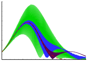
Figure 4 shows the effect of $\bar {h}$, which measures the distance between the two plates, on the linear evolution of the mode. For moderate values of $\bar {h}$ (1 and 2), the oscillations are significant in both the upstream and downstream regions. As $\bar {h}$ increases, the feedback effect is not obvious in the upstream region, but kicks in later in the downstream region. It is expected that the linear modal evolution with feedback reduces to the case of no reflection (represented by a Gaussian distribution) as $\bar {h}\rightarrow \infty$. This is confirmed by the comparison in figure 5, which indicates that the solutions with $\bar {h}=50$ and $20$ overlap with the Gaussian in a fairly large range. However, the feedback effect will still appear eventually in the region further downstream due to the finite value of $\bar {h}$, but that region is not relevant to the present theory. Figure 5(b) shows that the solution with $\bar {h}=10$ oscillates about the Gaussian in the downstream region, indicating that the feedback effect remains in action, albeit being much reduced.

Figure 4.

(a) Effects of $\bar {h}$ on the solution to the linear feedback equation (3.20) with $a_0=1$. (b) Zoom-in to the range $40<\bar {x}<50$ in (a).

Figure 5.

(a) The solution to the linear feedback equation (3.20) with $a_0=1$ and comparison with that for large values of $\bar {h}$ as well as the case of no reflection. (b) Zoom-in to the range $40<\bar {x}<50$ in (a).

The nonlinear feedback equation (3.16) is solved numerically for a moderate value of $\bar {h}$, and the results are shown in figure 6, where two grid sizes are employed to ensure satisfactory accuracy.

Figure 6.

Resolution check on the solution to the nonlinear feedback equation (3.16) with $a_0=3$ and $\bar {h}=2$. The step size of ‘Grid2’ is half of that of ‘Grid1’.

To see how nonlinearity affects the solutions with feedback, we fix $\bar {h}=2$ and vary the initial amplitude $a_0$ when solving the linear and nonlinear feedback equations (3.20) and (3.16). These results are displayed in figure 7. As expected, there is little difference between the linear and nonlinear solutions for $a_0=1$ (figure 7a). As the magnitude of $a_0$ increases, nonlinear effects are no longer negligible. For $a_0=3$, the nonlinear and linear solutions are qualitatively similar but there is appreciable quantitative difference, with the amplitude acquiring a larger value under the influence of nonlinearity (figure 7b). For $a_0=3.65$, a qualitative difference is observed: the nonlinear solution develops a singularity at a finite distance, $\bar {x}_s$ say, while the linear counterpart attenuates, and so does the nonlinear one without feedback (figure 7c). Dictated by the nonlinear term, the singularity is of the form (Leib Reference Leib1991),

(3.27)\begin{equation} A\rightarrow a_\infty (\bar{x}_s-\bar{x})^{-(5/2+\mathrm{i}\phi_s)} \quad\mbox{as}\ \bar{x}\rightarrow\bar{x}_s, \end{equation}

where $\phi _s$ and $a_\infty$ are constants. Increasing further the initial amplitude to $a_0=5$, the nonlinear solutions with and without feedback both blow up, with the former exhibiting oscillations, whereas the linear solution still undergoes highly oscillatory attenuation (figure 7d).

Figure 7.

Effects of the initial amplitude $a_0$ on the solution to the nonlinear feedback equation (3.16) with $\bar {h}=2$, for (a) $a_0=1$, (b) $a_0=3$, (c) $a_0=3.65$, (d) $a_0=5$. Thick solid lines indicate solution to (3.16); thin solid lines indicate solution to (3.20); dashed lines indicate nonlinear solution without feedback.

Next, we evaluate the effects of $\bar {h}$ on the nonlinear solution with feedback. Figure 8(a) shows that when $a_0=3$, the solutions for all five non-zero $\bar {h}$ are bounded. The feedback causes rapid oscillations. For large values of $\bar {h}$ (e.g. 5), the feedback effect is not obvious in the upstream region, but becomes significant later in the downstream region. As $\bar {h}$ is reduced, the feedback effect becomes significant in both the upstream and downstream regions, causing oscillations about the solution without reflection (figure 8b). Increasing further the magnitude of $a_0$, the solutions for various values of $\bar {h}$ all terminate at a finite-distance singularity but in an oscillatory manner, as is shown in figures 8(c,d).

Figure 8.

Effects of $\bar {h}$ on the solution to the nonlinear feedback equation (3.16) for (a) $a_0=3$ and (c) $a_0=5$. (b,d) Zoom-in plots for the ranges $60<\bar {x}<80$ and $-15<\bar {x}<0$ in (a,c), respectively.

For the antisymmetric case with small initial amplitude, the solution to the linear feedback equation

(3.28)\begin{equation} A^{\prime}(\bar{x})=\sigma\bar{x} A-R^{1/2}\mathscr{C}_F\,A(\bar{x}-\chi\bar{h}), \end{equation}

together with the initial condition (3.19), can be obtained numerically, or evaluated using the analytical solution, which corresponds to (3.26) with the sign in the second term in the exponent being changed to positive. The effects of $\bar {h}$ on the linear and nonlinear solutions turn out to be, by and large, similar to those of the symmetric case, hence they are not presented.

3.2. The coupled equations

We now consider the system of the coupled equations (3.9), taking the case of $\bar {h}=2$ for illustration. For each fixed total amplitude

(3.29)\begin{equation} \check{a}_0\equiv \sqrt{(a^{+}_0)^2+(a^{-}_0)^2}, \end{equation}

we vary the amplitude ratio $a^{+}_0/a^{-}_0$. Figure 9 shows the evolution of the coupled modes with different initial amplitude ratios for $\check {a}_0=1$, which is sufficiently small that nonlinearity is unimportant in the entire course of the development. Figure 9(a) depicts the evolution of the two modes for $a^{+}_0/a^{-}_0=0$. In this case, mode $A^{+}$, initially unseeded, is excited by mode $A^{-}$ through the Mach wave radiated by the latter. Mode $A^{+}$ starts to grow downstream even though in the upstream region its amplitude is rather small. Due to the nature of coupling, mode $A^{+}$ also reaches a peak at a downstream position, and in turn affects the evolution of mode $A^{-}$, resulting in small oscillations of its amplitude in the downstream region. The development of the coupled modes for the case $a^{+}_0/a^{-}_0=0.3$ is shown in figure 9(b). The amplitudes of both modes, $A^{+}$ and $A^{-}$, attenuate in the downstream region after attaining their respective maxima. Mode $A^{-}$ grows first and is followed by decay with minor oscillations, while mode $A^{+}$ exhibits strong oscillations due to the impact of the stronger mode $A^{+}$. When $a^{+}_0/a^{-}_0=0.7$, both modes $A^{+}$ and $A^{-}$ experience notable oscillations as they evolve downstream (figure 9c). Figure 10 shows the evolution of the coupled modes in the case $\check {a}_0=3.6$, for which nonlinearity becomes important but does not cause blow-up yet. The trend of the evolution is similar to the case $\check {a}_0=1$, that is, the feedback effect, manifested as oscillations, becomes more appreciable as the amplitude ratio increases. Another feature is that the envelope of the mode is strongly distorted due to nonlinearity (figures 10a,b). In all three cases, the solutions indicate that the nonlinear interaction and coupling cause vigorous energy exchange between the two modes. The development of the coupled modes with different initial amplitude ratios for $\check {a}_0=5$ is shown in figure 11. When $a^{+}_0/a^{-}_0=0$ (figure 11a), mode $A^{-}$ rapidly develops a singularity at a finite distance while also exciting mode $A^{+}$, which blows up subsequently. It is interesting to note that the singularities of two modes are of the same form as (3.27) but do not appear simultaneously. Moreover, oscillations are hardly appreciable, indicating that in this case, nonlinearity becomes dominant; mode $A^{-}$ already terminates at a singularity before mode $A^{+}$ acquires an amplitude large enough to act back on $A^{-}$. As the amplitude ratio increases, oscillations develop on the amplitudes of both modes and become stronger before a finite-distance singularity occurs (figures 11b,c).

Figure 9.

Effects of the amplitude ratio on the solution to the coupled equations (3.9) with $\bar {h}=2$ and $\sqrt {(a^{+}_0)^2+(a^{-}_0)^2}=1$, for (a) $a^{+}_0/a^{-}_0=0$, (b) $a^{+}_0/a^{-}_0=0.3$, (c) $a^{+}_0/a^{-}_0=0.7$.

Figure 10.

Effects of the amplitude ratio on the solution to the coupled equations (3.9) with $\bar {h}=2$ and $\sqrt {(a^{+}_0)^2+(a^{-}_0)^2}=3.6$, for (a) $a^{+}_0/a^{-}_0=0$, (b) $a^{+}_0/a^{-}_0=0.3$, (c) $a^{+}_0/a^{-}_0=0.7$.

Figure 11.

Effects of the amplitude ratio on the solution to the coupled equations (3.9) with $\bar {h}=2$ and $\sqrt {(a^{+}_0)^2+(a^{-}_0)^2}=5$, for (a) $a^{+}_0/a^{-}_0=0$, (b) $a^{+}_0/a^{-}_0=0.3$, (c) $a^{+}_0/a^{-}_0=0.7$.

3.3. Evolution with large values of $\mathscr {C}_F$

The amplitude equation (3.9) describing the coupling of the radiating modes in two supersonic boundary layers through acoustic feedback is in fact generic, and may arise in other types of flows. For example, the effective coupling may take place in two supersonic planar or circular jets, since each also radiates highly directional Mach waves (Tam Reference Tam1995; Wu Reference Wu2005). While the magnitude of the coefficient $\mathscr {C}_F$ measuring the effect of coupling in the present twin boundary layer is $O(10^{-3})$ and rather moderate, it could be much larger in other flows, e.g. twin jets, since the radiation turned out to be stronger (Wu Reference Wu2005). In view of this, we study the the amplitude equation with feedback for artificially increased $\mathscr {C}_F$.

By fixing $\mathscr {C}_F=3\times 10^{-2}$ and keeping other parameters unchanged, we perform a numerical study of (3.16). With typical Reynolds number remaining as $R=10^4$, the magnitude of the coefficient of the feedback term, $R^{1/2}|\mathscr {C}_F|$, is found to be $O(1)$. Figure 12 shows the solution to (3.16) for different $\bar {h}$. For $a_0=3$, the feedback effect is significant even for $\bar {h}$ as large as 15, causing the amplitude to undergo strong and rapid oscillations (figures 12a,b). A notably different feature is that with a larger $\bar {h}$, e.g. $\bar {h}=15$, the envelope of the amplitude attenuates to an almost diminished level and then resurrects. This resurgence is due to the enlarged feedback effect, by which the emitted sound wave re-excites the mode, at a later time due to substantial delay. For $a_0=5$ (figures 12c,d), the solutions for different $\bar {h}$ all blow up, with oscillations resembling those in the case of moderate $|\mathscr {C}_F|$ (cf. figures 8c,d).

Figure 12.

Effects of $\bar {h}$ on the solution to the nonlinear feedback equation (3.16) for (a) $a_0=3$ and (c) $a_0=5$, with $\mathscr {C}_F=3\times 10^{-2}$. (b,d) Zoom-in plots for the ranges $80<\bar {x}<100$ and $-10<\bar {x}<0$ in (a,c), respectively.

4. Cousin boundary layers

We now consider the case where the upper plate has a different surface temperature. A band of radiating modes may still exist on each boundary layer, but the nearly neutral modes do not have the same frequency and wavelength. In this case, for a radiating mode on the lower boundary layer, the upper boundary layer acts as a pure reflector with a finite reflection. We refer to these two boundary layers as ‘cousin boundary layers’, a configuration that is more general than the twin boundary layers, and more representative of practical applications. The distance between the two plates is still chosen as $h=O(R^{1/2})$ so that the upper and lower boundary layers share a common acoustic near field in the core. The reflection process is again described by the Cartesian coordinates $(x,y^{+})$/$(x,y^{-})$ for the upper/lower plate, as shown in figure 1.

The near-field Mach wave radiated from the lower boundary layer is given by (6.9) in Part 1, and can be written as (3.2), and setting $y^{-}=\bar {h}$ in this gives the incident sound wave upon the upper boundary layer:

(4.1)\begin{equation} p^{-}\rightarrow\epsilon\mathscr{C}_{\infty}\,A(\bar{x}-\chi\bar{h}) \exp({-\mathrm{i}\alpha q h})\exp({\mathrm{i}\alpha q y^{+}})\,E\equiv\epsilon R^{{-}1/2}p_I^+\exp({\mathrm{i}\alpha q y^{+}})\,E, \end{equation}

where we have put

(4.2)\begin{equation} p_I^{+}(\bar{x})=R^{1/2}\mathscr{C}_{\infty}\,A(\bar{x}-\chi\bar{h})\exp({-\mathrm{i}\alpha q h}). \end{equation}

The radiated Mach wave is reflected back to the lower boundary layer to act as an incident wave. The reflection process is similar to that considered in Part 1, and is described briefly here. In the main upper boundary layer, the disturbance has the expansion

(4.3)\begin{align} (\rho^{+}, u^{+}, v^{+}, p^{+}, \theta^{+}) &=\epsilon R^{{-}1/2}(\hat{\rho}^{+}_0, \hat{u}^{+}_0, \hat{v}^{+}_0, \hat{p}^{+}_0, \hat{\theta}^{+}_0)(\bar{x},y^{+})E \nonumber\\ &\quad+\epsilon R^{{-}1}(\hat{\rho}^{+}_1, \hat{u}^{+}_1, \hat{v}^{+}_1, \hat{p}^{+}_1, \hat{\theta}^{+}_1)+\mathrm{c.c.}+\cdots. \end{align}

Substitution of the above expansion into (2.2) in Part 1 followed by linearisation and elimination of $\hat {\rho }^{+}_0$, $\hat {u}^{+}_0$, $\hat {v}^{+}_0$ and $\hat {\theta }^{+}_0$ yields at leading order the Rayleigh equation for the pressure, $\mathscr {L}\hat {p}^{+}_0=0$, where the operator $\mathscr {L}$ is defined by (2.29) in Part 1. As $y^{+}\rightarrow \infty$,

(4.4)\begin{equation} \hat{p}^{+}_0\sim p_I^{+}(\bar{x})\left[\exp({\mathrm{i}\alpha q y^{+}})+\mathscr{R}\exp({-\mathrm{i}\alpha q y^{+}})\right], \end{equation}

where the reflection coefficient $\mathscr {R}$ is determined by performing a linear critical-layer analysis together with numerical integration as described in Part 1. At the next order, a routine calculation shows that the pressure $\hat {p}^{+}_1$ satisfies an inhomogeneous Rayleigh equation

(4.5) \begin{equation} \mathscr{L}\hat{p}^{+}_1=\frac{2\mathrm{i} c}{\alpha}\biggl\{ \frac{\bar{U}^\prime}{(\bar{U}-c)^2}\, \frac{\partial^2\hat{p}^{+}_0}{\partial\bar{x}\,\partial y^{+}} +\frac{\alpha^2}{c}\left[ \frac{M^2\bar{U}(\bar{U}-c)}{\bar{T}}-1 \right] \frac{\partial\hat{p}^{+}_0}{\partial\bar{x}} \biggr\}-\bar{x}\varDelta^{+}, \end{equation}

where

(4.6) \begin{align} \varDelta^{+}&=\biggl\{ \frac{2\bar{U}^\prime}{\bar{U}-c}\biggl( \frac{\bar{U}_1}{\bar{U}-c}-\frac{\bar{U}_1^\prime}{\bar{U}^\prime} \biggr) +\frac{\bar{T}^\prime}{\bar{T}}\biggl( \frac{\bar{T}_1^\prime}{\bar{T}^\prime}-\frac{\bar{T}_1}{\bar{T}} \biggr) \biggr\} \frac{\partial\hat{p}^{+}_0}{\partial y^{+}}\nonumber\\ &\quad +\alpha^2 M^2\,\frac{(\bar{U}-c)^2}{\bar{T}}\left( \frac{2\bar{U}_1}{\bar{U}-c}-\frac{\bar{T}_1}{\bar{T}} \right) \hat{p}^{+}_0. \end{align}

As $y^{+}\rightarrow \infty$,

(4.7)\begin{align} \hat{p}^{+}_1&\sim\hat{p}_I(\bar{x})\,[\exp({\mathrm{i}\alpha q y^{+}})+\hat{\mathscr{R}}(\bar{x})\exp({-\mathrm{i}\alpha q y^{+}})]\nonumber\\ &\quad +q^{{-}1}[M^2(1-c)-1]\,p_I^{+\prime}(\bar{x})\,y^{+}(\exp({\mathrm{i}\alpha q y^{+}})-\mathscr{R}\exp({-\mathrm{i}\alpha q y^{+}})). \end{align}

Evidently, the main-layer expansion breaks down when $y^{+}=O(R^{1/2})$, thus we introduce $\bar {y}^{+}=R^{-1/2}y^{+}$ corresponding to the common acoustic region. The perturbation now expands as

(4.8) \begin{align} (\rho^{+}, u^{+}, v^{+}, p^{+}, \theta^{+}) &=\epsilon R^{{-}1/2}(\rho^{+}_0, u^{+}_0, v^{+}_0, p^{+}_0, \theta^{+}_0)\nonumber\\ &\quad +\epsilon R^{{-}1}(\rho^{+}_1, u^{+}_1, v^{+}_1, p^{+}_1, \theta^{+}_1)+\cdots. \end{align}

At leading order, the pressure $p^{+}_0$ satisfies the wave equation $\mathscr {L}_w p^{+}_0=0$, with the operator $\mathscr {L}_w$ being given by (6.1) in Part 1. The solution takes the form

(4.9)\begin{equation} p^{+}_0=\check{p}_{\mathcal{I}}(\bar{x},\bar{y}^{+})\exp({\mathrm{i}\alpha(x-ct+qy^{+})}) +\check{p}_{\mathcal{R}}(\bar{x},\bar{y}^{+})\exp({\mathrm{i}\alpha(x-ct-qy^{+})})+\mathrm{c.c.}, \end{equation}

where $\check {p}_{\mathcal {I}}$ and $\check {p}_{\mathcal {R}}$ are to be determined by considering the second-order term $p^{+}_1$, which is governed by the equation

(4.10) \begin{equation} \mathscr{L}_w p^{+}_1 =2\biggl[ \frac{\partial^2 p^{+}_0}{\partial\bar{x}\,\partial{x}}+\frac{\partial^2 p^{+}_0}{\partial\bar{y}^{+}\,\partial y^{+}} -M^2\left( \frac{\partial}{\partial{t}}+\frac{\partial}{\partial{x}} \right)\frac{\partial p^{+}_0}{\partial\bar{x}} \biggr]. \end{equation}

To remove the secular terms in the expansion, we must require that the term proportional to $p^{+}_0$ on the right-hand side of the above equation be zero. Moreover, matching with the main-layer solution leads to

(4.11)\begin{equation} \left.\begin{gathered} {[M^2(1-c)-1]}\frac{\partial\check{p}_{\mathcal{I}}}{\partial\bar{x}} -q\,\frac{\partial\check{p}_{\mathcal{I}}}{\partial\bar{y}^{+}} = 0, \\ \check{p}_{\mathcal{I}}(\bar{x},\bar{y}^{+})=p_I^{+}(\bar{x}) \quad\mbox{at}\ \bar{y}^{+} = 0, \end{gathered}\right\} \end{equation}

and

(4.12)\begin{equation} \left.\begin{gathered} {[M^2(1-c)-1]}\frac{\partial\check{p}_{\mathcal{R}}}{\partial\bar{x}} +q\,\frac{\partial\check{p}_{\mathcal{R}}}{\partial\bar{y}^{+}} = 0, \\ \check{p}_{\mathcal{R}}(\bar{x},\bar{y}^{+})=\mathscr{R}p_I^{+}(\bar{x}) \quad\mbox{at}\ \bar{y}^{+} = 0. \end{gathered}\right\} \end{equation}

The solution to (4.11) is $\check {p}_{\mathcal {I}}(\bar {x},\bar {y}^{+})=p_I^{+}(\bar {x}+\chi \bar {y}^{+})$, which is the radiated wave from the lower boundary layer since

(4.13) \begin{align} \epsilon & R^{{-}1/2}\,\check{p}_{\mathcal{I}}(\bar{x},\bar{y}^{+})\exp({\mathrm{i}\alpha(x-ct+qy^{+})}) \nonumber \\ & \quad =\epsilon\mathscr{C}_{\infty}\,A(\bar{x}+\chi\bar{y}^{+}-\chi\bar{h})\exp({-\mathrm{i}\alpha q h}) \exp({\mathrm{i}\alpha q y^{+}})\,E \nonumber \\ & \quad =\epsilon\mathscr{C}_{\infty}\,A(\bar{x}-\chi\bar{y}^{-})\exp({-\mathrm{i}\alpha q y^{-}})\,E =\epsilon p^{-}_0, \end{align}

which is exactly (3.2). The solution to (4.12) is $\check {p}_{\mathcal {R}}(\bar {x},\bar {y}^{+})=\mathscr {R}\,p_I^{+}(\bar {x}-\chi \bar {y}^{+})$. This solution represents the outgoing wave for the upper boundary layer, and serves as the incident wave for the lower boundary layer. We can write

(4.14)\begin{align} p_{\mathscr{R}}^{+}&\equiv\epsilon R^{{-}1/2}\,\check{p}_{\mathcal{R}}(\bar{x},\bar{y}^{+})\exp({\mathrm{i}\alpha(x-ct-qy^{+})})\nonumber\\ & =\epsilon\mathscr{R}\mathscr{C}_{\infty}\,A(\bar{x}-\chi\bar{y}^{+}-\chi\bar{h}) \exp({-\mathrm{i}\alpha q h})\exp({-\mathrm{i}\alpha q y^{+}})\,E \nonumber\\ & =\epsilon\mathscr{R}\mathscr{C}_{\infty}\,A(\bar{x}-\chi\bar{y}^{+}-\chi\bar{h}) \exp({-2\mathrm{i}\alpha q h})\exp({\mathrm{i}\alpha q y^{-}})\,E. \end{align}

As $\bar {y}^{+}\rightarrow \bar {h}$, the reflected wave by the upper boundary layer has the form

(4.15)\begin{align} p_{\mathscr{R}}^{+}\rightarrow\epsilon\mathscr{R}\mathscr{C}_{\infty}\,A(\bar{x}-2\chi\bar{h})\exp({-2\mathrm{i}\alpha q h}) \exp({\mathrm{i}\alpha q y^{-}})\,E\equiv\epsilon R^{{-}1/2}\,p_I^{-}(\bar{x})\exp({\mathrm{i}\alpha q y^{-}})\,E, \end{align}

where we have put

(4.16)\begin{equation} p_I^{-}(\bar{x})=R^{1/2}\mathscr{R}\mathscr{C}_{\infty}\,A(\bar{x}-2\chi\bar{h})\exp({-2\mathrm{i}\alpha q h}). \end{equation}

Substitution of the above expression into the amplitude equation (4.61) and use of the composite amplitude equation (5.10) in Part 1 leads to

(4.17)\begin{align} A^{\prime}(\bar{x}) &= \sigma\bar{x} A+ \varUpsilon R^{2/3}\int_{0}^{\infty}\!\int_{0}^{\infty} K(\xi,\eta;\bar{s})\, A(\bar{x}-c\xi)\,A(\bar{x}-c\xi-c\eta) \nonumber\\ &\quad\times A^{*}(\bar{x}-2c\xi-c\eta)\,{\rm d}\eta\,{\rm d}\xi +R^{1/2}\mathscr{C}_R\mathscr{R}\,A(\bar{x}-2\chi\bar{h}), \end{align}

where

(4.18)\begin{equation} \mathscr{C}_R=2\alpha^2 q\mathscr{C}^{2}_{\infty}\exp({-2\mathrm{i}\alpha q h})/[c(1-c)^2G], \end{equation}

comparison of which with (3.8) shows that $|\mathscr {C}_R|=|\mathscr {C}_F|$. Similar to the twin boundary layers, the acoustic feedback contributes a linear term with delay (which is twice as long). The initial condition is found as

(4.19)\begin{equation} A(\bar{x})=a_0\left[ \exp({\sigma\bar{x}^2/2}) -\frac{R^{1/2}\mathscr{C}_R\mathscr{R}}{2\sigma\chi\bar{h}}\exp({\sigma(\bar{x}-2\chi\bar{h})^2/2}) \right] \quad\mbox{as}\ \bar{x}\rightarrow -\infty. \end{equation}

Since the coefficient $\mathscr {C}_R\mathscr {R}$ in the amplitude equation (4.17) measures the importance of the reflection-facilitated feedback effect, we first evaluate its dependence on the base-flow parameters. Figures 13(a,c,e) show the variation of $\mathscr {C}_R\mathscr {R}$ with the upper wall temperature $T^+_w$ for several values of fixed lower wall temperature $T^-_w$ at different Mach numbers. In each case, the coefficient $\mathscr {C}_R\mathscr {R}$ remains more or less constant and small (being of $O(10^{-3})$), but increases rapidly when approaching the resonant temperature ($T^+_w=T^-_w$), at which point $\mathscr {C}_R\mathscr {R}$ becomes infinite. Figures 13(b,d, f) show the variation of $\mathscr {C}_R\mathscr {R}$ with the lower wall cooling ratio $r^-_c$ for fixed upper wall temperature $T^+_w$ at Mach numbers $M=5$, $6$ and $7$. In each case, $r^-_c$ is varied in the full range where a radiating mode exists. There is no significant difference of $\mathscr {C}_R\mathscr {R}$ for various $T^+_w$ except for $T^+_w$ that is in the range of the existence of the radiating mode, e.g. $T^+_w=2.5$, $3$ and $3.5$ for $M=5$, $6$ and $7$, respectively. For such values of $T^+_w$, $\mathscr {C}_R\mathscr {R}$ raises quickly in a narrow range of $r^-_c$, which contains $T^+_w=T^-_w$, at which resonance takes place and correspondingly $\mathscr {C}_R\mathscr {R}$ becomes unbounded.

Figure 13.

The coefficient $\mathscr {C}_R\mathscr {R}$ versus (a,c,e) the upper wall temperature $T^+_w$ and (b,d, f) the lower wall cooling ratio $r^-_c$, for Mach numbers (a,b) $M=5$, (c,d) $M=6$ and (e, f) $M=7$. The ranges of the existence of the radiating mode are $r^-_c\in [0.457,0.582]$ ($T^-_w\in [2.37,3.02]$), $r^-_c\in [0.403,0.494]$ ($T^-_w\in [2.83,3.47]$) and $r^-_c\in [0.36,0.427]$ ($T^-_w\in [3.3,3.92]$) for $M=5$, $6$ and $7$, respectively.

4.1. Effects of upper wall temperature

We first calculate the reflection coefficient $\mathscr {R}$ for different upper wall temperatures $T^+_w$ with a given Mach number $M=6$ and fixed lower wall temperature $T^-_w=3$. The magnitude of the reflection coefficient turns out to be almost unity for most upper wall temperatures, except that it increases rapidly when the wall temperature corresponding to the resonant case ($T^+_w=T^-_w=3$) is approached. Using these results, we perform a numerical study of the amplitude equation (4.17) for different $T^+_w$ with $M=6$ and $T^-_w=3$. Three representative initial amplitudes are considered: $a_0=3$, for which nonlinearity just becomes appreciable, $a_0=3.6$, for which nonlinearity becomes significant but the solution remains bounded (and finally attenuates), and $a_0=5$, in which case the solution blows up. Figures 14(a,b) show that for the two moderate values of $a_0$ ($3$ and $3.6$), the acoustic feedback induces oscillations to the amplitude of the supersonic mode, similar to the case of a twin boundary layer even though the feedback is now facilitated through the reflected Mach wave emitted by the same boundary layer. The amplitude evolution appears much the same for various $T^+_w$, with small differences being just visible in the enlarged views. With initial amplitude $a_0=5$ (figure 14c), the solutions all blow up, with the feedback effect manifested as barely appreciable oscillations, and the effect of $T^+_w$ on the evolution is also negligible.

Figure 14.

Effects of the upper wall temperature $T^+_w$ on the solution to the amplitude equation (4.17) with $\bar {h}=2$, for (a) $a_0=3$, (b) $a_0=3.6$, (c) $a_0=5$. Here, $T^+_w=7.02$ corresponds to the adiabatic wall condition. The lower wall temperature is $T^-_w=3$, and the Mach number is $M=6$.

Figure 15 shows the nonlinear evolution of the radiating mode in the lower boundary layer when the upper and lower wall temperatures are close ($T^+_w\approx T^-_w= 3$). Figure 15(a) compares the modal evolution for different $T^+_w$ with $a_0=3$, where nonlinearity is moderate. It is seen that the mode amplitude for different $T^+_w$ oscillates about the solution without reflection. As $T^+_w$ approaches $T^-_w$ (i.e. nearly satisfies the resonant condition), the oscillations become more intense due to the rapid increase of the reflection coefficient. This is also true for $a_0=3.6$, for which the nonlinear effect becomes enhanced but without causing a finite-distance singularity (figure 15b). When $a_0=5$ (figure 15c), all the solutions blow up in an oscillatory manner, with oscillations becoming more pronounced closer to the resonant condition. The present theory ceases to be applicable when the temperatures of the two walls are extremely close, and instead needs to be reformulated as a ‘detuned’ twin-boundary-layer model.

Figure 15.

Strong oscillations of the solution to the amplitude equation (4.17) with $\bar {h}=2$ when the upper wall temperature $T^+_w$ approaches the lower wall temperature $T^-_w=3$, for (a) $a_0=3$, (b) $a_0=3.6$, (c) $a_0=5$. The Mach number is $M=6$.

While much attention has been paid to linear radiating modes, whose radiating characteristics have been fairly well understood, back effects of the radiated sound on their linear and nonlinear evolution have not been studied previously. There exist no experimental or computational data with which our theoretical predictions could be compared. Nevertheless, we noted, upon completion of the present work, that recently Chen, Wang & Fu (Reference Chen, Wang and Fu2021) employed the method of linear parabolised stability equations to trace the development of radiating modes in a hypersonic boundary layer over a wedge. They found that the amplitude underwent considerable oscillations (see e.g. figure 15(c) in the paper), despite the facts that no rigid reflecting surface was present and that a monotonic amplification or decay was predicted by linear stability theory. This puzzling outcome was attributed to the beating effect of multiple coexisting modes, which may be amplifying or damped. An alternative but more plausible explanation, based on the main finding of the present work, could be that the shock, which is present in their problem, acts to reflect the spontaneously radiated sound, thereby establishing an acoustic back action akin to what was studied here. Our assertion is also based upon the realisation that an amplitude equation of the same form as (4.17) can be derived in the case of reflection by a shock. It is worth noting that an imperfect non-reflecting far-field boundary condition in numerical calculations could also cause similar behaviour, which would of course be an artefact. This implies that for numerical methods to capture faithfully and accurately the radiating mode and its evolution, it is important to specify an appropriate far-field condition. Numerical simulations to validate the theoretical findings would be a major undertaking and are deemed beyond the scope of the present study. We hope that our theoretical work would prompt computational and experimental studies.

4.2. Evolution with large values of $\mathscr {C}_R$

Again, the magnitude of the coefficient $\mathscr {C}_R$ representing the effect of coupling may be larger in certain types of flows, e.g. a supersonic jet adjacent to a reflecting surface, which mimics a jet engine installed on a wing (Cavalieri et al. Reference Cavalieri, Jordan, Wolf and Gervais2014; Lyu et al. Reference Lyu, Dowling and Naqavi2017). An amplitude equation similar to (4.17) can be derived, but stronger Mach wave radiation could lead to a greater $\mathscr {C}_R$. With this perspective in mind, we now solve the amplitude equation (4.17) for an artificially increased $\mathscr {C}_R$, i.e. $\mathscr {C}_R=3\times 10^{-2}$. We now take a somewhat large $\bar {h}=7$, for which the feedback effect may be significant, as will be seen, and keep other parameters unchanged. Figure 16 shows the effects of $T^+_w$ on the nonlinear evolution of the radiating mode in the lower boundary layer. For $a_0=3$ and $3.6$, the results are displayed in figures 16(a,b). In addition to the usual rapid oscillations of the amplitude, the envelope of the amplitude features a second peak in the downstream region. The resurrection after the mode is nearly extinct is again due to the enlarged feedback term in (4.17), which re-excites the radiating mode after a fairly long delay. The zoomed views in figures 16(a,b) indicate that strong cooling (e.g. $T^+_w=0.5,2$) or the adiabatic condition ($T^+_w=7.02$) results in a smaller second peak compared with the cases $T^+_w=4$ and $5$, but the overall difference is barely appreciable. For the case $a_0=5$, the amplitude rapidly blows up within a finite distance due to the nonlinear effect, which is dominant over the acoustic feedback such that the latter plays hardly any role (figure 16c), and in this case the solution is little influenced by $T^+_w$.

Figure 16.

Effects of the upper wall temperature $T^+_w$ on the solution to the amplitude equation (4.17) with ${\bar {h}=7}$ and $\mathscr {C}_R=3\times 10^{-2}$, for (a) $a_0=3$, (b) $a_0=3.6$, (c) $a_0=5$. Here, $T^+_w=7.02$ corresponds to the adiabatic wall condition. The lower wall temperature is $T^-_w=3$, and the Mach number is $M=6$.

5. Summary and conclusions

In this paper, we investigated linear and nonlinear evolution of supersonic instability modes under the back action of the Mach waves radiated spontaneously by the modes themselves. This scenario of acoustic feedback was considered in the simplest setting of two supersonic boundary layers developing along two semi-infinite parallel plates. The distance separating the two plates is assumed to be comparable with the transverse extent of the near field of the Mach waves, a configuration representative of the combustion chamber of a scramjet. Using the formula for the Mach wave radiation in the near field, the amplitude equations are derived for two cases of relevance: the twin boundary layers and cousin boundary layers.

For the so-called twin boundary layers, where the wall conditions are identical, the Mach wave radiated from the instability mode in one boundary layer impacts that in the other. This process is described by a system of coupled amplitude equations, in which the contribution of the back effects enters in the form of a linear term of delay type. In the special cases where the modes in the two boundary layers are in symmetric and antisymmetric phases, the system reduces to a single-amplitude equation. The system of the coupled amplitude equations, including its reduced forms, was studied analytically and numerically. The evolution characteristics were found to depend on the distance between the plates, measured by the rescaled distance $\bar {h}$, as well as on the initial amplitudes of the supersonic modes and their ratio. For moderate values of $\bar {h}$, the primary effect of the acoustic feedback is to induce rapid oscillations of the modal amplitudes, which remain bounded for small or moderate initial amplitudes, but blow up (i.e. develop a singularity at finite distances) when the initial amplitudes are large enough. The feedback plays a destabilising role in general, enhancing the modal amplitude, causing singularity which is otherwise absent, and in the extreme case of a supersonic mode being seeded in only one boundary layer exciting the supersonic mode in the other. The ratio of the initial amplitudes changes the evolution significantly, and specifically renders the blow-up to occur at different downstream locations. In the limit of the rescaled plate separation $\bar {h}\rightarrow \infty$, the evolution reduces, as expected, to the case of no acoustic back effect.

In the more general case of the so-called cousin boundary layers, where the wall temperatures are different, the spontaneously emitted Mach wave by the supersonic mode in one of the boundary layers is reflected back by the other to affect the original radiating mode. The amplitude equation was derived, which consists of a linear term of delay type representing the acoustic feedback. Since the amplitude equation is rather similar to those in the case of twin boundary layers, the acoustic feedback plays a similar role, namely, causes the amplitude to oscillate rapidly. It is found that if the wall temperature is not too close to the resonant condition, then the reflection coefficient is almost a constant and hence the development of the instability mode appears the same. However, if the wall temperature is close to the resonant condition, then the reflected wave becomes stronger than the Mach wave originally emitted, resulting in greater feedback effects on the modal evolution, which manifest as strong oscillations of the modal amplitude.

The amplitude equations pertinent to twin and cousin boundary layers could arise in other situations, such as twin jets or a jet adjacent to a rigid surface, where the feedback effect may be stronger. In view of such broad applications, we also solved the amplitude equations with the coefficients of the feedback terms being increased by one order of magnitude. The acoustic feedback effect turns out to be still significant for fairly large $\bar {h}$. With longer delays of the feedback action, the amplitude of the instability mode not only exhibits rapid oscillations, but also experiences near extinction followed by resurrection, which occurs due to the sound wave emitted earlier re-exciting the supersonic mode at a later time.

The present theoretical investigation provides physical insights into how the spontaneously radiated Mach waves and the instability modes could be effectively coupled in double supersonic boundary layers. The results are deemed useful for assessing the impact of the noise emitted from the tunnel walls on the supersonic mode evolving in the boundary layer over the test model. They are probably relevant also for instability and transition in scramjet combustion chambers as well as for twin-jet engines or jet engines installed in the vicinity of a surface (wing or fuselage).