


1. Introduction
When a cylindrical duct featuring an axisymmetric cavity is subject to a turbulent air flow, hydrodynamic instabilities appear in the shear layer between the fast flow in the duct and the air at rest in the cavity. The unsteady vorticity associated with these instabilities forces the acoustic modes of the cavity, which in turn perturb the shear layer, thus closing a potentially unstable aeroacoustic feedback loop. Such whistling phenomena have been studied extensively in the cases of shallow and deep side-branch cavities (e.g. East Reference East1966; Elder, Farabee & Demetz Reference Elder, Farabee and Demetz1982; Yamouni, Sipp & Jacquin Reference Yamouni, Sipp and Jacquin2013; Bourquard, Faure-Beaulieu & Noiray Reference Bourquard, Faure-Beaulieu and Noiray2021; Pedergnana et al. Reference Pedergnana, Bourquard, Faure-Beaulieu and Noiray2021), and also in the case of axisymmetric cavities (e.g. Aly & Ziada Reference Aly and Ziada2010; Nakiboğlu, Manders & Hirschberg Reference Nakiboğlu, Manders and Hirschberg2012; Oshkai & Barannyk Reference Oshkai and Barannyk2013; Abdelmwgoud, Shaaban & Mohany Reference Abdelmwgoud, Shaaban and Mohany2020; Wang & Liu Reference Wang and Liu2020). In the latter situations, and when the cavity is deep, as in the present work, the first azimuthal acoustic modes are often involved. These azimuthal aeroacoustic instabilities can be a critical problem in the design of piping systems, valves, turbomachines, boilers or heat exchangers. Moreover, they exhibit strong similarities to thermoacoustic instabilities in annular and axisymmetric combustors, where the driving mechanism originates from the unsteady heat release rate of the flames instead of the unsteady vorticity: in both types of systems, high-amplitude azimuthal oscillations can develop in the form of spinning, standing, mixed or beating acoustic waves (see for instance the papers from Aly & Ziada Reference Aly and Ziada2011; Abdelmwgoud et al. Reference Abdelmwgoud, Shaaban and Mohany2020; Faure-Beaulieu et al. Reference Faure-Beaulieu, Indlekofer, Dawson and Noiray2021; Indlekofer et al. Reference Indlekofer, Faure-Beaulieu, Noiray and Dawson2021).
In the present two-part study, an azimuthal aeroacoustic instability in a deep axisymmetric cavity subject to a turbulent pipe flow is studied experimentally and theoretically in order to explain the underlying governing mechanisms. While Reference Faure-Beaulieu, Xiong, Pedergnana and NoirayPart 1 focuses on the influence of the aeroacoustic oscillations on the onset of a mean swirling motion of the flow, we investigate in the present Part 2 the effect of a swirling mean flow on the dynamics of the aeroacoustic azimuthal modes. These phenomena have not been considered in the literature so far. More specifically, here, we aim at answering the following questions:
(i) Do the azimuthal aeroacoustic modes spin with or against the mean swirl?
(ii) Which mechanisms cause a preference for a specific spinning direction?
(iii) Are the existing low-order models for azimuthal thermoacoustic instabilities sufficient to describe the aeroacoustic modal dynamics of axisymmetric cavity flows?
Regarding the first question, the cavity is investigated experimentally with acoustic measurements and stereoscopic particle image velocimetry (PIV). The set-up features tangential inlets, which allow us to adjust the intensity of a counterclockwise (CCW) swirl upstream of the cavity. A reconstruction of the spatio-temporal evolution of the acoustic pressure field around the cavity reveals the existence of a statistical preference for different spinning directions, depending on the swirl intensity.
Regarding the second question, let us briefly discuss the different physical mechanisms that can promote one spinning direction over the other. A first mechanism is the difference of stability between the hydrodynamic modes spinning with and against the mean swirl direction. As in the studies of Gallaire & Chomaz (Reference Gallaire and Chomaz2003b) and Oberleithner, Paschereit & Wygnanski (Reference Oberleithner, Paschereit and Wygnanski2014), we will perform a linear stability analysis of the incompressible swirling mean flow to determine if the least stable hydrodynamic modes spin with or against the flow. Besides, in recent studies on the analogue problem of thermoacoustic instabilities in annular combustion chambers, it was shown that the presence of reflectional and rotational asymmetries in the system influences the spinning direction of the modes (e.g. Bauerheim, Cazalens & Poinsot Reference Bauerheim, Cazalens and Poinsot2015; Faure-Beaulieu et al. Reference Faure-Beaulieu, Indlekofer, Dawson and Noiray2021). We will show that this second mechanism also plays an important role in the preferred spinning direction of the present aeroacoustic modes. A third mechanism that influences the spinning direction of the modes is the feedback phenomenon of emerging mean swirl due to spinning aeroacoustic waves, explained in Reference Faure-Beaulieu, Xiong, Pedergnana and NoirayPart 1. The respective contribution of these three mechanisms will be elucidated in the present work.
Regarding the third question, we propose to describe the modal dynamics observed in the experiments with a low-order time-domain model based on nonlinear amplitude and phase equations and time scale separation. Models of this type have been developed and used for a long time to study thermoacoustic instabilities in solid rocket engines (Yang, Kim & Culick Reference Yang, Kim and Culick1976; Awad & Culick Reference Awad and Culick1983; Culick Reference Culick1987) and more recently to develop gas turbine combustors for power generation and aviation (e.g. Indlekofer et al. Reference Indlekofer, Faure-Beaulieu, Dawson and Noiray2022). They generally include polynomial expansions to model the nonlinear heat release rate response of the flames to acoustic perturbations, which often lead to stable limit cycles. Such models are also convenient to describe hydrodynamic instabilities (Zhu, Gupta & Li Reference Zhu, Gupta and Li2017; Lee et al. Reference Lee, Zhu, Li and Gupta2019) and aeroacoustic instabilities (Boujo et al. Reference Boujo, Bourquard, Xiong and Noiray2020; Bourquard et al. Reference Bourquard, Faure-Beaulieu and Noiray2021). However, a specificity of the present configuration is the complex reciprocal interaction between the azimuthal aeroacoustic modes and the mean swirling flow. Our starting point will be the equations derived by Faure-Beaulieu & Noiray (Reference Faure-Beaulieu and Noiray2020) to which new elements will need to be added to account for this interaction.
The structure of this Part 2 paper is as follows: §§ 2 and 3 describe respectively the experimental set-up and operating conditions, and the dynamics of the aeroacoustic modes. In § 4, an analysis based on the linearised Navier–Stokes equations (LNSE) reveals how the eigenvalues of the shear layer eigenmodes spinning in co-swirl and counterswirl directions split when the swirl intensity is varied. Section 5 is dedicated to the derivation of the low-order model. Section 6 compares the results of the time-domain simulations from the model with the experimental observations.
2. Experimental set-up
The experimental set-up is presented in figures 1(a) and 1(b). It consists of a cylindrical wind channel of diameter  $D=40$ mm and length 1570 mm, featuring in its centre an axisymmetric cavity of radius $R=128$ mm and width $W=30$ mm, with at its up- and downstream ends anechoic terminations reflecting less than 2 % of incident acoustic energy above 300 Hz. As shown in figure 1(d), a blower injects air at $20\,^\circ {\rm C}$ in the upstream anechoic termination. The axial air mass flow $\dot {m}$ is manually controlled with a valve and monitored with a mass flow meter. Tangential air injection can be imposed from four 1 cm diameter pipes (see figure 1a) to induce a swirling flow. The direction of this swirl is CCW when looking from downstream. The mass flow injected in this swirler is denoted by $\dot {m}_s$ and the total mass flow in the wind channel is $\dot {m}_t = \dot {m} + \dot {m}_s$.

Figure 1. (a) Sketch of the wind channel equipped with a swirler located upstream of the axisymmetric cavity. The axial air mass flow is denoted by  $\dot {m}$, and $\dot {m}_s$ is the tangential mass flow injected in the swirler. (b) Dimensions of the cavity. (c) Position of the microphones measuring the acoustic pressure at the inner wall the cavity. (d) Sketch of the overall experimental set-up showing the anechoic terminations up- and downstream of the wind channel. (e) Mean flow velocity profiles in the middle of the cavity, obtained from stereoscopic PIV for $\dot {m}=84\ {\rm g}\ {\rm s}^{-1}$ ( $U_x=59\ {\rm m}\ {\rm s}^{-1}$) and $\dot {m}_s=0\ {\rm g}\ {\rm s}^{-1}$. The dotted line in the panel showing $\bar {u}_x$ presents the mirrored profile for $y<0$ in order to highlight the presence of small asymmetries of the mean axial velocity.
The acoustic pressure is measured with several microphones in the cavity and along the channel: six are flush-mounted on the downstream wall of the axisymmetric cavity at  $r=90$ mm and $\varTheta =0^\circ, 28^\circ, 90^\circ,152^\circ,208^\circ,270^\circ,332^\circ$ (see figure 1c), allowing the reconstruction of the acoustic pressure field of the first azimuthal modes at any instant. Two additional microphones at $\varTheta =135^\circ$ are placed at radial positions $r=67.5$ mm and $r=121.5$ mm in order to identify the radial distribution of the modes. Microphones that are flush mounted on the wind channel's wall up- and downstream of the cavity allow us to quantify the exponential amplitude decay of the azimuthal acoustic modes, which are trapped in the cavity and evanescent in the wind channel.
Figure 1(e) shows the three components of the mean velocity profile in the centre of the cavity for  $\dot {m}=84\ {\rm g}\ {\rm s}^{-1}$, which corresponds to a bulk velocity $U_x=59\ {\rm m}\ {\rm s}^{-1}$, and without imposed mean swirl ( $\dot {m}_s=0$). These profiles were obtained with stereoscopic PIV (more details about the experimental set-up are given in Reference Faure-Beaulieu, Xiong, Pedergnana and NoirayPart 1). In the left panel showing the mean axial velocity profile $\bar {u}_x$, the thin dotted line in the upper half is a mirrored profile of $\bar {u}_x(y)$ for $y<0$, which reveals a small unintended rotational asymmetry of the configuration. The upstream section of the wind channel is not long enough to obtain a perfectly axisymmetric fully developed turbulent flow, and this slight asymmetry of the mean axial velocity in the cavity is attributed to the presence of the upstream tangential injection holes or to remnant non-uniformities of the velocity profile caused by the U-turn upstream of the convergent (see figure 1d).
We also observe a non-zero mean flow in the out-of-plane  $z$ direction, although no swirl was imposed upstream of the cavity ( $\dot {m}_s=0$). This azimuthal mean flow in the cavity is induced, as explained in Reference Faure-Beaulieu, Xiong, Pedergnana and NoirayPart 1, by the strong aeroacoustic instability at $U_x=59\ {\rm m}\ {\rm s}^{-1}$. The characteristics of this wave-induced swirl depend on the amplitude, the intermittency and the spinning component of the aeroacoustic wave. In particular, for low-amplitude self-sustained azimuthal modes, which exhibit frequent changes of spinning component's direction due to the inherent forcing from turbulence, no significant emerging mean swirl is detected.
3. Experimental observations
3.1. Azimuthal aeroacoustic instability
In the range  $60 < \dot {m} < 100\ {\rm g}\ {\rm s}^{-1}$, which corresponds to $42< U_x < 70\ {\rm m}\ {\rm s}^{-1}$, the system presents an aeroacoustic instability involving the first azimuthal acoustic mode and a shear layer mode of azimuthal order 1. It is characterised by the shedding of large vortices that span across the cavity's width $W$ (see Reference Faure-Beaulieu, Xiong, Pedergnana and NoirayPart 1). The whistling frequency does not vary much over the whole range of bulk velocities: it starts at 773 Hz when $U_x = 42\ {\rm m}\ {\rm s}^{-1}$ and reaches 809 Hz when $U_x = 70\ {\rm m}\ {\rm s}^{-1}$. Figure 2(b) shows the acoustic pressure field associated with the first pure azimuthal mode in the analogue geometry of a cylindrical chamber. In this simplified case, the Helmholtz eigenvalue problem can be solved analytically and the shapes of the first pair of degenerate azimuthal eigenmodes are $p(r,\varTheta )={\rm J}_1(rZ_1/R)\cos (\varTheta )$ (represented in the figure) and $p(r,\varTheta )={\rm J}_1(rZ_1/R)\sin (\varTheta )$, where ${\rm J}_1$ is the Bessel function of the first kind and order 1, and $Z_1$ is the first zero of ${\rm J}_1'$. The corresponding frequency is 786 Hz, which is in agreement with the experimental results.

Figure 2. (a) Measured acoustic pressure signals for  $\dot {m}=84\ {\rm g}\ {\rm s}^{-1}$ ( $U_x=59\ {\rm m}\ {\rm s}^{-1}$) and $\dot {m}_s=0$. (b) Instantaneous acoustic pressure field associated with the first pure azimuthal acoustic mode of a cylindrical cavity, obtained analytically. The eigenfrequency is 786 Hz.
Figure 2(a) shows acoustic signals recorded simultaneously by three cavity microphones at different azimuthal positions and equal distance from the axis: the colours of the lines correspond to the colours of the microphones in the sketch 1(c). These signals were recorded for  $\dot {m} = 84\ {\rm g}\ {\rm s}^{-1}$ ( $U_x=59\ {\rm m}\ {\rm s}^{-1}$) and $\dot {m}_s=0$, a condition at which a high-amplitude aeroacoustic limit cycle at 790 Hz is present, reaching an acoustic level of 165 dB. The long time interval displayed in this figure does not allow us to see the details of the quasi-sinusoidal oscillations at 790 Hz, but it shows the fluctuations of the acoustic pressure envelope which are largely caused by the forcing from turbulence. On the yellow time trace ( $\varTheta =332^\circ$), one can see at $t\approx 15$ s some quasi-periodic modulation of the acoustic envelope, corresponding to a beating azimuthal mode, i.e. cyclic alternation of clockwise (CW) and CCW mixed modes with a period lasting a few hundreds of acoustic periods. This deterministic phenomenon of self-sustained beating modes was recently discovered and explained in the case of thermoacoustic instabilities in combustion chambers by Faure-Beaulieu et al. (Reference Faure-Beaulieu, Indlekofer, Dawson and Noiray2021). The yellow time trace is also characterised by sporadic high-amplitude bursts which can reach 8000 Pa for a few seconds.
3.2. Modal projection of the acoustic field
Interpreting the raw acoustic signals is not straightforward. It is therefore convenient to use the quaternion projection proposed by Ghirardo & Bothien (Reference Ghirardo and Bothien2018) on the basis of the work of Flamant, Le Bihan & Chainais (Reference Flamant, Le Bihan and Chainais2017), in order to unravel the modal dynamics. This projection can be used to describe the acoustic pressure field associated with an azimuthal wave of any order and it is particularly suited to providing a straightforward and unambiguous interpretation of the corresponding thermoacoustic time series (Ghirardo & Bothien Reference Ghirardo and Bothien2018). It writes as
 \begin{align} p_a=A\cos(m(\varTheta-\theta))\cos(\chi)\cos(\omega t + \varphi) + A\sin(m(\varTheta-\theta))\sin(\chi)\sin(\omega t + \varphi),\end{align}
where  $m$ is the azimuthal order of the mode – in the present study, it is always equal to 1. In (3.1), $\varTheta$ is the azimuthal coordinate, $t$ is the time and $\omega$ is the angular frequency of the oscillations. This ansatz is referred to as the ‘quaternion projection’ because it is the real part of a quaternion analytical signal (Flamant et al. Reference Flamant, Le Bihan and Chainais2017)
 \begin{equation} p_a={\rm Re}\big(A \mathrm{e}^{\mathrm{i} m(\varTheta-\theta)}\mathrm{e}^{-\mathrm{k}\chi}\mathrm{e}^{\mathrm{j}(\omega t + \varphi)}\big), \end{equation}
where  $\mathrm {i}$, $\mathrm {j}$ and $\mathrm {k}$ are the basic quaternions and $A(t)$, $\chi (t)$, $\theta (t)$ and $\varphi (t)$ are the four slow variables which define the instantaneous state of the mode. The positive variable $A$ is the amplitude of the acoustic pressure. The nature angle $\chi$ indicates the type of mode: if $\chi =0$, the mode is purely standing; if $\chi ={\rm \pi} /4$, it is purely CCW spinning; if $\chi =-{\rm \pi} /4$, it is purely CW spinning; if $0<\chi <{\rm \pi} /4$, it is a CCW mixed mode that can be decomposed as the superposition of a pure standing mode and a pure CCW spinning mode; if $0>\chi >-{\rm \pi} /4$, it is CW mixed mode. The angle $\theta$ indicates the orientation of the maximal acoustic pressure amplitude: for a standing mode, $\theta$ is simply the antinodal direction. For a mixed mode, it is the antinodal direction of the standing component of the mode. For a pure spinning mode, $\theta$ transforms into a temporal phase information. The last variable, $\varphi$, is a temporal phase that can be associated with small fluctuations of the acoustic period $2{\rm \pi} /\omega$. The four variables $A$,
$A$,  $\chi$, $\theta$ and $\varphi$ are useful to represent variations of the instantaneous mode state, which are slow compared with the acoustic period, i.e. $\dot {A}/A$, $\dot {\chi }$, $\dot {\theta }$ and $\dot {\varphi }$ are much smaller than $\omega$.
To perform the quaternion projection, the prescribed frequency  $\omega$ must be close to the frequency of the instability. It is usually not appropriate to define $\omega$ as the frequency of the pure acoustic mode, because it can noticeably differ from the aeroacoustic mode frequency due to the time delay of the shear layer response and the presence of small flow asymmetries (Noiray, Bothien & Schuermans Reference Noiray, Bothien and Schuermans2011; Kim et al. Reference Kim, John, Adhikari, Wu, Emerson, Acharya, Isono, Saitoh and Lieuwen2022). The most adequate option is usually to choose $\omega$ as the frequency of the dominant peak in the power spectral density.
Furthermore, the expression (3.1) describes the dependence of the acoustic field along the spatial coordinate  $\varTheta$ only. This one-dimensional (1-D) description is readily applicable to the case of thin annular combustors (Faure-Beaulieu & Noiray Reference Faure-Beaulieu and Noiray2020), and it can also be used for azimuthal modes exhibiting non-uniform distribution of the acoustic pressure in the axial and radial direction, i.e. $A=A(t,x,r)$. Indeed, in such situation, the three-dimensional (3-D) acoustic field can be spatially averaged over constant $\varTheta$ planes as explained in Appendix A. All the six microphones used for the quaternion projection are located at the same radial and axial positions and the full 3-D acoustic field can be reconstructed from the measured amplitudes and the knowledge of the mode shape.
3.3. Effect of an imposed swirl on the aeroacoustic mode
Acoustic measurements were performed for different levels of swirl by increasing  $\dot {m}_s$ from 0 to $21\ {\rm g}\ {\rm s}^{-1}$ by steps of $3\ {\rm g}\ {\rm s}^{-1}$ while keeping a constant total mass flow $\dot {m}_t=84\ {\rm g}\ {\rm s}^{-1}$ (Reynolds number ${Re}=1.5\times 10^{5}$). The corresponding mean azimuthal velocity remains moderate compared with the axial velocity: PIV measurements in the cavity show a maximal local value of $15\ {\rm m}\ {\rm s}^{-1}$ when $\dot {m}_s=18\ {\rm g}\ {\rm s}^{-1}$, while the mean axial bulk velocity is $U_x=59\ {\rm m}\ {\rm s}^{-1}$. This gives a swirl number of 0.18, which is relatively small compared with the values usually found in the literature on swirling flows (e.g. Gallaire & Chomaz Reference Gallaire and Chomaz2003b; Qadri, Mistry & Juniper Reference Qadri, Mistry and Juniper2013; Oberleithner et al. Reference Oberleithner, Paschereit and Wygnanski2014; Tammisola & Juniper Reference Tammisola and Juniper2016).
The frequency of the aeroacoustic instability is not substantially affected by the imposed swirl and remains between 790 and 797 Hz. To characterise the influence of the imposed swirl on the aeroacoustic limit cycle, the state variables  $A$,
$A$,  $\chi$, $\theta$ and $\varphi$ are extracted from the acoustic time series following the procedure described by Ghirardo & Bothien (Reference Ghirardo and Bothien2018). Figure 3 presents the evolution of the state variables for $\dot {m}_s=0$, 3, 6 and $9\ {\rm g}\ {\rm s}^{-1}$ (from left to right). The cases $\dot {m}_s>9\ {\rm g}\ {\rm s}^{-1}$, not shown here, behave similarly as for $\dot {m}_s=9\ {\rm g}\ {\rm s}^{-1}$. Let us now describe the dynamics of the slow state variable at these four conditions.

Figure 3. Evolution of the slow state variables  $A$,
$A$,  $\chi$, $\theta$ and $\varphi$ extracted from the experimental acoustic measurements, for different swirl numbers imposed on the flow upstream of the axisymmetric cavity. The four tangential mass flows $\dot {m}_s$ considered in columns (a–d) are equal to 0, 3, 6 and $9\ {\rm g}\ {\rm s}^{-1}$ respectively for a total mass flow $\dot {m}_t$ kept constant and equal to $84\ {\rm g}\ {\rm s}^{-1}$.
For  $\dot {m}_s=0$, which is shown in figure 3(a), the evolution of the nature angle $\chi$ indicates intermittent transitions between a CCW mixed mode with $\chi \approx {\rm \pi}/8$ and a beating mode characterised by quasi-periodic changes of the spinning direction that manifest themselves by triangular oscillations of $\chi$. These two regimes can last several seconds, which is long compared with the acoustic period ( $\approx$1.25 ms) and the characteristic time of growth of an aeroacoustic instability. The amplitude $A$ displays large bursts in mixed mode regime, and stays around 5 kPa in the beating regime. Faure-Beaulieu et al. (Reference Faure-Beaulieu, Indlekofer, Dawson and Noiray2021) showed that beating can be caused by small non-uniformities in the geometry, the impedance of the cavity walls or the flow. The small asymmetry of the mean axial velocity profile reported earlier is thus a possible explanation for the occurrence of beating in the present configuration. In the mixed mode regime, the preferred orientation $\theta$ undergoes small stochastic fluctuations around a fixed angle defined modulo ${\rm \pi}$, while during the beating regime, it shows periodic square oscillations.
When  $\dot {m}_s=3\ {\rm g}\ {\rm s}^{-1}$, the mixed mode regime and its high-amplitude bursts disappear, and only the beating mode regime is observed (figure 3b). The fast drift of $\varphi$ is explained by the mismatch between the frequency $\omega$ chosen for the quaternion projection and the actual dominant aeroacoustic frequency during the considered time interval. For this case, the aeroacoustic dynamics shows no preference for the CW or CCW spinning direction, which is confirmed by the probability density function (p.d.f.) of $\chi$ in figure 4. The symmetry of the aeroacoustic dynamics is recovered because the small imposed swirl compensates the effect of the small inherent reflectional asymmetry of the system. The reflectional symmetry of the aeroacoustic dynamics, which manifests itself here as a robust beating mode without preference for the CW or the CCW spinning direction, is therefore recovered by imposing a small mean swirl, i.e. imposing a small reflectional asymmetry to the system. In summary, inherent imperfections are present in the system, as in the case of thermoacoustic instabilities investigated by Faure-Beaulieu et al. (Reference Faure-Beaulieu, Indlekofer, Dawson and Noiray2021). They lead to a dominant CCW mixed mode in absence of mean swirl ( $\dot{m}_s= 0\ {\rm g}\ {\rm s}^{-1}$), and this dominance is eliminated by imposing a small swirl on the incoming flow ( $\dot{m}_s= 3\ {\rm g}\ {\rm s}^{-1}$, and $\dot{m}_s/\dot{m}_t = 3.5\,\%$).

Figure 4. Experimental p.d.f. of the nature angle  $\chi$ for the same conditions as in figure 3, for increasing imposed swirler mass flow $\dot {m}_s=0$, 3, 6 and $9\ {\rm g}\ {\rm s}^{-1}$ (darker shades correspond to stronger swirl). Each p.d.f. is obtained from acoustic time traces of 100 s. Values of $-{\rm \pi} /4$, $0$ and ${\rm \pi} /4$ correspond respectively to the states of pure CW spinning wave, pure standing wave and pure CCW spinning wave.
When the swirler mass flow is further increased to  $\dot {m}_s=6\ {\rm g}\ {\rm s}^{-1}$ (figure 3c), the dynamics of the state variables become similar to the case $\dot {m}_s=0$, except that the preferred spinning direction is CW instead of CCW. Indeed, a sporadic alternance of mixed CW regime and beating regime is observed, indicating that the imposed swirl tends to promote the CW, i.e. counterswirl direction. Finally, when $\dot {m}_s=9\ {\rm g}\ {\rm s}^{-1}$, the beating regime disappears, leaving only a CW spinning mode of amplitude of 8 kPa (figure 3d). For higher values of $\dot {m}_s$, the mode keeps spinning in the same counterswirl direction.
Figure 4 summarises the evolution of the p.d.f. of  $\chi$ for the four experimental conditions presented in figure 3. Darker lines indicate higher swirler mass flows $\dot {m}_s$. Without swirl, the p.d.f. is bimodal and asymmetric, with a higher peak for a positive value of $\chi$ and a smaller peak for a negative $\chi$. At $\dot {m}_s=3\ {\rm g}\ {\rm s}^{-1}$, the p.d.f. has two symmetric peaks indicating that there is no longer a preference for one spinning direction. The p.d.f. for $\dot {m}_s=6\ {\rm g}\ {\rm s}^{-1}$ is almost the mirror image of the case without swirl, with a preference for CW mixed modes. For $\dot {m}_s=9\ {\rm g}\ {\rm s}^{-1}$, the p.d.f. has a single, sharp peak, very close to $\chi =-{\rm \pi} /4$ (quasi-pure CW spinning mode). In order to explain these observations, it is therefore key to separately investigate the effects of the mean flow on the aeroacoustic wave and the ones of the wave on the mean flow. The latter mechanism is the topic of Reference Faure-Beaulieu, Xiong, Pedergnana and NoirayPart 1, and the former is treated in the present Part 2.
4. Hydrodynamic stability of the simulated mean swirling flow
In this section, we investigate how a mean swirl impacts the stability of spinning hydrodynamic modes in the shear layer, depending on their spinning direction with respect to the swirl. To that end, we use the framework developed in Reference Faure-Beaulieu, Xiong, Pedergnana and NoirayPart 1, which is based on the linearised Navier–Stokes equations (LNSE) for small perturbation analysis around turbulent incompressible mean flows (e.g. Pujals et al. Reference Pujals, Garcia-Villalba, Cossu and Depardon2009; Iungo et al. Reference Iungo, Viola, Camarri, Porté-Agel and Gallaire2013; Beneddine et al. Reference Beneddine, Sipp, Arnault, Dandois and Lesshafft2016; Tammisola & Juniper Reference Tammisola and Juniper2016; Boujo, Bauerheim & Noiray Reference Boujo, Bauerheim and Noiray2018).
The shear layer can be considered as incompressible for the following reasons: (i) the Mach number of the wind channel flow is small ( ${Ma}=U_x/c=59/340=0.17$, where $c$ is the speed of sound), (ii) the cavity width (3 cm) and the maximal shear layer thickness (2 cm) are small compared with the acoustic wavelength (43 cm). This allows us to proceed with an incompressible LNSE framework in order to describe the shear layer dynamics when it is subject to the forcing from the acoustic mode. Furthermore, the excellent agreement between the compressible large eddy simulations and the incompressible LNSE predictions of the forced response of a shear layer in the 2-D counterpart of the present axisymmetric configuration performed by Boujo et al. (Reference Boujo, Bauerheim and Noiray2018) validates the rationale of this approach. Still, it is important to stress that it is not possible to predict the frequency and the linear growth rate of the aeroacoustic modes of the system with this incompressible analysis, and that the prediction of the stability of these modes would necessitate a more involved framework based on the compressible LNSE.
Bearing all this in mind, we aim at identifying the dominant incompressible hydrodynamic modes involved in the aeroacoustic instability and at estimating their decay rates and pure hydrodynamic frequencies depending on their spinning direction.
For such an axisymmetric configuration, the LNSE in the frequency domain, which constitutes a linear eigenvalue problem in infinite dimension, can be expanded as a Fourier series in the azimuthal direction and can be solved with a finite element discretisation. It allows us to separately investigate the eigenfunctions of any given azimuthal order. Here, only the dominant hydrodynamic modes of azimuthal order  $m=-1$ (CCW spinning waves) and $m=+1$ (CW spinning wave) are considered, because, as shown in Part I, these are the modes which constructively interact with the first azimuthal acoustic mode. Their helical structure spins around the shear layer that spans the cavity opening, and the size of the corresponding vortices is of the order of the cavity width.
As in Reference Faure-Beaulieu, Xiong, Pedergnana and NoirayPart 1, we perform the LNSE analysis with a partial mean flow, which is computed from the incompressible Reynolds-averaged Navier–Stokes (RANS) equations. We do not use a mean flow obtained experimentally with stereoscopic PIV for the following reasons: (i) the experimental field of view is too restrained to perform reliable LNSE, in particular the boundary conditions of the domain are not properly defined; (ii) for the entire range of  $\dot {m}_t$ considered in this work, the experiments show a strong aeroacoustic limit cycle, which is associated with a substantial thickening of the mean shear layer induced by the high-amplitude hydrodynamic oscillations, as in the 2-D analogue geometry investigated by Boujo et al. (Reference Boujo, Bauerheim and Noiray2018).
The axisymmetric RANS simulations are performed on the same 2-D domain as in Reference Faure-Beaulieu, Xiong, Pedergnana and NoirayPart 1. A non-zero azimuthal velocity  $U_a$ is imposed over a small rectangular region ( $2\ {\rm cm}\times 1\ {\rm cm}$ in longitudinal and radial directions) located in the wind channel 70 cm upstream of the cavity to mimic the effect of the tangential injectors in the experimental configuration. A positive value of $U_a$ corresponds, as in the experiments, to a CCW swirl. The tangential velocity $U_a$ is varied between 0 and $5\ {\rm m}\ {\rm s}^{-1}$ by steps of $1\ {\rm m}\ {\rm s}^{-1}$ to obtain the six axisymmetric mean flows with different amounts of swirl intensities. The inlet's axial velocity profile is uniform and fixed to ensure a constant mass flow of $84\ {\rm g}\ {\rm s}^{-1}$ at the outlet for each case.
Figure 5(a) shows, in the complex plane, the eigenvalues of the dominant hydrodynamic eigenmodes of order  $m=+1$ and $m=-1$ for these six mean flows. The imaginary part is the mode's angular frequency and the real part, its linear growth rate. The colour of the symbols corresponds to the swirl strength, with cyan being the case without swirl ( $U_a=0\ {\rm m}\ {\rm s}^{-1}$), and pink being the case with the strongest swirl ( $U_a=5\ {\rm m}\ {\rm s}^{-1}$). The circles and crosses respectively correspond to $m=-1$ and $m=+1$.

Figure 5. Dominant eigenvalues of the LNSE problems defined by axisymmetric RANS flows with and without swirl ( $U_a=0\ {\rm m}\ {\rm s}^{-1}$ and $U_a=[1,\dots,5]\ {\rm m}\ {\rm s}^{-1}$, with $U_x=59\ {\rm m}\ {\rm s}^{-1}$). Without swirl, there is a pair of degenerate eigenmodes which have the same eigenvalue and spin in opposite directions. With swirl, this pair of eigenvalues splits, i.e. the co- and counterswirl hydrodynamic modes do not exhibit the same frequency and decay rate. (a) The LNSE spectra of modes of azimuthal order $-1$ ( $\circ$, CCW) and $+1$ ( $\times$, CW) when the azimuthal velocity $U_a$ in the tangential injector is increased from 0 to $5\ {\rm m}\ {\rm s}^{-1}$. (b,c) Frequencies and growth rates of the leading shear layer eigenmodes when the azimuthal flow velocity in increased.
All the eigenvalues have a negative real part, which indicates that the RANS axisymmetric flow is globally stable. As explained in Reference Faure-Beaulieu, Xiong, Pedergnana and NoirayPart 1, most of the eigenvalues are clustered along branches in the complex plane which are not shown here. These are strongly damped modes exhibiting spatial distribution in the axisymmetric cavity or the channel. However, a pair of eigenvalues typically emerges above these branches, corresponding to shear layer modes which are significantly less damped than all the other modes in the same range of frequency. Consequently, if the flow is subject to harmonic forcing in this range, its response will be governed by these shear layer modes.
When  $U_a=0$, the shear layer eigenmodes $m=1$ and $m=-1$ are degenerate, i.e. they share the eigenvalue $\lambda = 6849\,\mathrm {i}-1024$. When $U_a$ is increased, the shear layer mode $m=-1$ drifts to the right and downwards in the complex plane, while the mode $m=+1$ drifts to the left and upwards. Figures 5(b) and 5(c) show separately the evolution of the frequency and the growth rate of the two modes as function of $U_a$. The frequency of the mode of order $-1$ increases almost linearly with $U_a$, while the frequency of the mode of order $1$ decreases linearly. These trends are expected, because the mode of order $-1$, spinning in the swirl direction, propagates faster around the cavity, while the mode of order $+1$, spinning against the swirl, propagates slower. The splitting of the linear decay rates of the incompressible shear layer eigenmodes shown in figure 5(c), reveals that the co-swirl eigenmode becomes more damped with $U_a$ while the counterswirl is less damped.
These results show that adding a mean swirl to the incoming pipe flow promotes the counterswirl incompressible hydrodynamic eigenmodes by making them less linearly stable than the co-swirl eigenmodes, which explains the experimental observations of dominant self-sustained counterswirl aeroacoustic modes.
We now quantify the dependence of the frequency splitting on the swirl, with the aim to include it in the low-order model of the next section. From the data presented in figures 5(b) and 5(c), it appears that the frequency split  $\Delta f=\,f_{CCW}-f_{CW}$ and the growth rate split $\Delta \sigma =\sigma _{CCW}-\sigma _{CW}$ are both proportional to $U_a$, with the following linear relationships $\Delta f=5.2 \, U_a$ and $\Delta \sigma =-8.9\,U_a$. The speeds of the co- and counterswirl aeroacoustic waves can be written as $c+U_{\varTheta \,{sl}}$ and $c-U_{\varTheta \,{sl}}$, with $U_{\varTheta \,{sl}}$ an effective azimuthal convective velocity in the shear layer. Considering that $\Delta f$ scales with the velocity difference of the waves as $\Delta f/f_0 = 2 U_{\varTheta \,{sl}}/c$, with $f_0$ the eigenfrequency in absence of mean swirl, one deduces that $\Delta \sigma = -8.9/5.2\times 2 U_{\varTheta \,{sl}}f_0/c$.
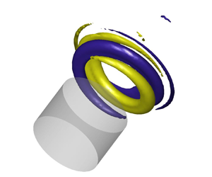
Figure 6 shows 3-D isosurfaces of the shear layer modes in presence of a mean swirl, for  $m=1$ and $m=-1$. These modes exhibit a helical structure, respectively winding with the swirl direction (indicated by a red arrow) and against it, and growing in the axial direction due to a convective shear layer instability, although the incompressible mean flow is globally stable.

Figure 6. Radial velocity isosurfaces of the dominant (a) counterswirl and (b) co-swirl eigenmodes obtained from the incompressible LNSE. The velocity imposed in the tangential injection is  $U_a=5\ {\rm m}\ {\rm s}^{-1}$. The swirl direction is indicated by the red arrow. Yellow and indigo surfaces respectively correspond to a positive value and its opposite.
Let us now briefly put these findings into perspective with some key results from the literature on hydrodynamic instabilities of incompressible swirling jets. The main mechanisms causing the emergence of weakly damped or linearly unstable helical modes in swirling flows are the axial and azimuthal shear between the fast swirling core and the surrounding air at rest, and the centrifugal instability (Gallaire & Chomaz Reference Gallaire and Chomaz2003a). Interestingly, Gallaire & Chomaz (Reference Gallaire and Chomaz2003b) show that, for low Reynolds swirling jets of small or moderate swirl, the convectively unstable mode with the largest temporal growth rate is, as in the present study, a helical mode of azimuthal order  $+1$ winding with the flow and spinning against it (note that, in their paper, the sign convention for $m$ is different). They also find that for the considered base flows, this mode is absolutely stable, i.e. perturbations at a given position are amplified, but they are advected sufficiently fast downstream to prevent a local growth of the oscillation amplitude. However, their incompressible stability analysis of canonical swirling jets differs in three main respects from the present work:
(i) In contrast to our global stability analysis, their results are obtained from a local one with the assumption of weakly non-parallel base flows.
(ii) Their swirling jets are not confined in the axial direction, while the finite width $W$ of the axisymmetric cavity considered in our study imposes a significant constraint on the structure and dynamics of the hydrodynamic modes.
(iii) In our study, the flow is highly turbulent, with a Reynolds number more than two orders of magnitude larger than in their study, and we perform a perturbation analysis around a partial mean flow being a solution of the incompressible RANS equations – ‘partial’ in the sense that it does not feature the effect of coherent motion due to the aeroacoustic instability – and not around a base flow being a steady solution of the incompressible Navier–Stokes equations.

Regarding the first two points, it is important to stress that the assumption of a weakly non-parallel flow is not valid at the upstream and downstream corners of the axisymmetric cavity. This fact limits the applicability of local stability analysis to our partial mean flow. This limitation also applies to the recent work of Douglas, Emerson & Lieuwen (Reference Douglas, Emerson and Lieuwen2021), who elucidated the mode selection process in laminar, incompressible and unconfined swirling jets, including strongly non-parallel flow cases. Using a global stability analysis, they unravelled complex bifurcation diagrams, which exhibit several simultaneous attractors corresponding to modes of different azimuthal numbers, winding and spinning directions.
Regarding the third point, the intense turbulence of the pipe flow upstream of the cavity leads to a thickening of the mean shear layer and a turbulent viscosity field featuring maxima along the shear layer region that are more than two orders of magnitude larger than the kinematic viscosity (see for instance figure 9 in Reference Faure-Beaulieu, Xiong, Pedergnana and NoirayPart 1 for  $U_a=0\ {\rm m}\ {\rm s}^{-1}$). In the present configuration, the latter effect does not markedly influence the frequency and the structure of the eigenmodes, as in the 2-D analogue geometry investigated by Boujo et al. (Reference Boujo, Bauerheim and Noiray2018). However, it significantly enhances their damping, which contributes to the fact that, as in the turbulent swirling flows investigated by Oberleithner et al. (Reference Oberleithner, Paschereit and Wygnanski2014) and Tammisola & Juniper (Reference Tammisola and Juniper2016), there is no linearly unstable global mode.
5. Low-order model of the aeroacoustic dynamics
The objective of this section is to derive a low-order model of the complex 3-D aeroacoustic dynamics observed in the experiments, based on a 1-D acoustic wave equation with a source term representing the vortex sound interactions in the shear layer. As a first step, we make use of the experimental and numerical results to disentangle the acoustic and hydrodynamic components of the aeroacoustic flow and further set the scene for the low-order modelling.
5.1. Decomposition of the aeroacoustic field
The coherent velocity fluctuations  $\tilde {\boldsymbol {u}}$ are decomposed into an irrotational acoustic part $\boldsymbol {u}_a$, and a hydrodynamic part $\boldsymbol {u}_h$ which corresponds to the incompressible vortical motion of the shear layer: $\tilde {\boldsymbol {u}}=\boldsymbol {u}_a + \boldsymbol {u}_h$. Similarly, the coherent pressure fluctuations are written as $\tilde {p} = p_a + p_h$ where $p_a$ is the acoustic pressure and $p_h$ is the pseudo-sound associated with the coherent, incompressible and rotational velocity fluctuations. In the next paragraphs, we apply this decomposition to the present system and analyse the fields $\boldsymbol {u}_a$ and $p_h$.
Phase averaging applied to PIV measurements gives access to  $\tilde {\boldsymbol {u}}$ in the cavity's centre and the shear layer (see Reference Faure-Beaulieu, Xiong, Pedergnana and NoirayPart 1), while the microphones on the cavity walls give access to $\tilde {p}$ at discrete locations. To estimate the respective contributions of acoustics and hydrodynamics to $\tilde {p}$ and $\tilde {\boldsymbol {u}}$ at different locations, we consider the experimental results, together with the LNSE results and Helmholtz solver computations.
For  $U_x = 59\ {\rm m}\ {\rm s}^{-1}$, $\tilde {\boldsymbol {u}}$ can reach $50\ {\rm m}\ {\rm s}^{-1}$ in the shear layer. The pseudo-noise pressure $p_h$, which is of the order of $\rho U_x u_h$, is approximated by $\rho U_x \tilde {u}$. This leads to $p_h\approx 3$ kPa in the shear layer, which is not negligible compared with the typical pressure fluctuation amplitude of 5 kPa measured by the microphones. Figure 7(a) shows the distribution of $p_h$ associated with the first hydrodynamic shear layer mode of azimuthal order $m=-1$, scaled to correspond to velocity fluctuations of the order of $50\ {\rm m}\ {\rm s}^{-1}$. The pseudo-sound $p_h$ indeed reaches values of 3 kPa in the shear layer, but vanishes away from the shear layer and is negligible at the microphone's location, indicated with a black rectangle. Figure 7(b) shows the $p_a$ field of the first azimuthal (pure) acoustic mode, obtained from a Helmholtz solver simulation. Unlike $p_h$, $p_a$ reaches its maximal values at the outer wall of the cavity. Therefore, it can be assumed that the microphones measure only the acoustic contribution $p_a$.

Figure 7. (a) Pseudo-sound field associated with the first shear layer mode, from the incompressible LNSE analysis around the simulated RANS mean flow without swirl. The grey rectangle indicates the position of the microphones at  $r=90$ mm. (b) Acoustic pressure field of the first CCW spinning azimuthal acoustic mode at a frequency 793 Hz, obtained from a Helmholtz solver. The acoustic amplitude was imposed to match the measured data at the microphone location. The phase $\phi =0$ is chosen as the phase reference for which the acoustic pressure reaches its positive maximum in the upper half of the cavity. At $\phi ={\rm \pi} /2$, the slice shown in the figure coincides with the acoustic mode nodal plane and the acoustic pressure is 0 everywhere. The vertical dashed line indicates the position of the axial slices shown in figure 8. (c) Out-of-plane component $u_{az}$ of $\boldsymbol {u}_a$ for the same mode, at the same instant of the oscillation cycle. The acoustic pressure is in phase with the azimuthal acoustic velocity $u_{a\varTheta }$, which is characteristic of a travelling wave. (d,e) Vertical and axial components of $\boldsymbol {u}_a$ for the first CCW spinning azimuthal acoustic mode, with a phase difference ${\rm \pi} /2$ with respect to (b,c). Indeed, $u_{ay}$ and $u_{ax}$ are phase shifted by ${\rm \pi} /2$ with respect to $p_a$ and $u_{a\varTheta }$. Therefore, at $\phi =0$, they vanish in this slice.

Figure 8. Slices of the acoustic pressure and acoustic velocity fields (respectively colour and arrows) in the transverse plane of the axisymmetric configuration (see dashed line in figure 7) for a CCW spinning mode and a standing mode with orientation  $\theta =0$ at two different phase instants: $\phi =0 \mod 2{\rm \pi}$ and $\phi ={\rm \pi} /2 \mod 2{\rm \pi}$, with $\phi =\omega t + \varphi$ the instantaneous acoustic phase. These pure acoustic modes are obtained with a Helmholtz solver computation.
The figures 7(c), 7(d) and 7(e) show the three velocity components of the first azimuthal acoustic mode. They are represented in Cartesian coordinates, rather than in cylindrical coordinates, to facilitate their interpretation. The out-of-plane and vertical velocity components  $u_{az}$ and $u_{ay}$ are respectively related to the azimuthal and radial velocity components $u_{a\varTheta }$ and $u_{ar}$. A propagating 1-D acoustic wave of amplitude $p_a\sim 5\ {\rm kPa}$ has an acoustic velocity $u_a=p_a/\rho c=13\ {\rm m}\ {\rm s}^{-1}$, which matches well with the magnitude of the out-of-plane acoustic velocity fluctuations shown in figure 7(c), although the present configuration cannot be approximated by a simple 1-D closed waveguide as it can be done for thin annular combustion chambers (Faure-Beaulieu & Noiray Reference Faure-Beaulieu and Noiray2020). The 3-D nature of the acoustic field can also be seen in figure 8, which shows, on the left, the acoustic pressure and velocity fields of a spinning pure acoustic mode at phases $\phi =0$ and $\phi ={\rm \pi} /2$ of the cycle, and, on the right, these fields when the acoustic mode is standing. The vertical dashed black line in figure 8 corresponds to the slices shown in figures 7(b) and 7(c). At phase $\phi =0$, the velocity field in the vertical plane is orthogonal to this plane, and it is thus purely azimuthal. At phase ${\rm \pi} /2$, the vertical slice corresponds to the nodal line of the acoustic pressure, i.e. $p_a=0$ in this plane, and the velocity vector field corresponds to a downwards motion towards the bottom half of the cavity (see also figure 7d,e). This CCW spinning mode can be interpreted as the superposition of two standing modes with orientations $\theta =0$ and $\theta ={\rm \pi} /2$, which exhibit a phase lag of ${\rm \pi} /2$. It is interesting to stress that for the spinning mode, the acoustic azimuthal velocity and pressure are in phase, while for the standing mode, they exhibit a phase shift of ${\rm \pi} /2$.
One can also see in figure 7(d) that  $u_{ax}$ and $u_{ay}$ exhibit maxima of about $40\ {\rm m}\ {\rm s}^{{-1}}$ around the corners of the cavity openings, which are far above the magnitude of $u_{az}$. This effect, although real, is overestimated due to the inviscid fluid assumption of the present Helmholtz solver computation which leads to singularities in the potential field at sharp corners. The resolvent analysis performed by Boujo et al. (Reference Boujo, Bauerheim and Noiray2018) on the 2-D counterpart of the present axisymmetric geometry shows that the optimal volumetric forcing of the shear layer is located in the vicinity of the upstream corner. Therefore, the fast acoustic motion around the corner perturbs the shear layer very efficiently, if not optimally. The resulting hydrodynamic oscillations are then advected and amplified along the shear layer.
5.2. Aeroacoustic wave equation
The starting point of the derivation of a low-order model of the present axisymmetric aeroacoustic system is the 3-D wave equation with unsteady velocity source terms, presented in Appendix A of the paper by Faure-Beaulieu & Noiray (Reference Faure-Beaulieu and Noiray2020)
 \begin{equation} \dfrac{\partial^2 \tilde{p}}{\partial t^2} + 2\bar{\boldsymbol{u}}\boldsymbol{\cdot}\boldsymbol{\nabla}\dfrac{\partial \tilde{p}}{\partial t} - c^2\nabla^2 \tilde{p} = 2\rho c^2\boldsymbol{\nabla} \bar{\boldsymbol{u}}:\boldsymbol{\nabla}\tilde{\boldsymbol{u}}^\top, \end{equation}
where the air density  $\rho$ and speed of sound $c$ are assumed uniform in the cavity, and $:$ is the double dot product between two tensors, with the same convention as in Faure-Beaulieu & Noiray (Reference Faure-Beaulieu and Noiray2020). The focus of this previous study was on thermoacoustics, and therefore, the acoustic source term of interest was the one of the coherent heat release fluctuations $(\gamma -1)\partial \dot {\mathcal {Q}}/\partial t$, while the aeroacoustic source term $2\rho c^2\boldsymbol {\nabla } \bar {\boldsymbol {u}}:\boldsymbol {\nabla } \tilde {\boldsymbol {u}}^\top$ was neglected. Conversely, in the present study, only this term is considered. The acoustic pressure is described with the quaternion formalism
 \begin{align} p_a&={\rm Re}\big(A \mathrm{e}^{\mathrm{i}(\theta-\varTheta)} \mathrm{e}^{-\mathrm{k}\chi}\mathrm{e}^{\mathrm{j}(\omega t + \varphi)}\big)\equiv{\rm Re}(Ah)\nonumber\\ &=\tfrac{1}{2}( A h + A h^*)\nonumber\\ &=\tfrac{1}{2}\big( A \mathrm{e}^{\mathrm{i}(\theta-\varTheta)}\mathrm{e}^{-\mathrm{k}\chi}\mathrm{e}^{\mathrm{j}(\omega t + \varphi)} + A\mathrm{e}^{-\mathrm{j}(\omega t + \varphi)}\mathrm{e}^{\mathrm{k}\chi}\mathrm{e}^{-\mathrm{i}(\theta-\varTheta)} \big), \end{align}
where  $h^*$ is the conjugate of the unitary quaternion $h=\mathrm {e}^{\mathrm {i}(\theta -\varTheta )} \mathrm {e}^{-\mathrm {k}\chi }\mathrm {e}^{\mathrm {j}(\omega t + \varphi )}$. This non-commutative quaternion formalism can be directly used to describe an azimuthal wave in a 1-D wave guide, in which case $A,\chi,\theta,\varphi$ are solely functions of time and slowly vary with respect to the acoustic period $2{\rm \pi} /\omega$. For the present axisymmetric geometry, a spatial averaging operation detailed in Appendix A allows us to reduce the 3-D problem with $A=A(t,r,z)$ to a 1-D equation. The spatial averaging is performed over an elementary volume $(r,\varTheta,x)\in [0,R]\times [\varTheta -\delta \varTheta /2,\varTheta +\delta \varTheta /2]\times [-X_\infty,X_\infty ]$, with $X_\infty$ chosen sufficiently large to be out of the zone of influence of the acoustic mode, which is always possible due to the evanescent character of the mode in the duct. Taking the limit $\delta \varTheta \rightarrow 0$, a 1-D azimuthal wave equation is obtained for the acoustic pressure averaged over a slice $[0,R]\times [-X_\infty,X_\infty ]$, which is denoted by $\langle p_a\rangle$ and depends solely on $t$ and $\varTheta$
 \begin{equation} \dfrac{\partial^2 \langle p_a\rangle}{\partial t^2} + \alpha\dfrac{\partial \langle p_a\rangle}{\partial t} + 2\dfrac{U_{\varTheta\,{eff}}}{R}\dfrac{\partial \langle p_a \rangle}{\partial \varTheta\partial t} - \omega_a^2\dfrac{\partial^2 \langle p_a\rangle}{\partial \varTheta^2} = \mathcal{S} ,\end{equation}
which has a damping term  $\alpha \partial {\cdot }/\partial t$, a convective term $2(U_{\varTheta \,{eff}}/R)\partial ^2 {\cdot }/\partial \varTheta \partial t$ and a source term $\mathcal {S}$ resulting from the spatial averaging of the aeroacoustic source term $2\rho c^2\boldsymbol {\nabla } \bar {\boldsymbol {u}}:\boldsymbol {\nabla } \tilde {\boldsymbol {u}}^\top$.
5.3. Model of the aeroacoustic source term
The hydrodynamic component of the velocity  $\boldsymbol {u}_h$ provides the main contribution to the source term $\mathcal {S}$: indeed, the ratio between the spatial derivatives of $\boldsymbol {u}_a$ and $\boldsymbol {u}_h$ has the order of magnitude of the ratio between the shear layer thickness ( $\sim$1 cm) and the acoustic wavelength ( $\sim$0.4 m). Additionally, the zones of strong gradients of $\overline{\boldsymbol{u}}$ and $\boldsymbol {u}_h$ coincide, so that the product $\boldsymbol {\nabla }\bar {\boldsymbol {u}}:\boldsymbol {\nabla }\bar {\boldsymbol {u}}_h^\top$ is even greater compared with $\boldsymbol {\nabla }\bar {\boldsymbol {u}}:\boldsymbol {\nabla }\bar {\boldsymbol {u}}_a^\top$. Therefore, only the contribution of $\boldsymbol {u}_h$ is considered from now on. The developed expression of $\boldsymbol {\nabla } \bar {\boldsymbol {u}}:\boldsymbol {\nabla } \boldsymbol {u}_h^\top$ in cylindrical coordinates is
 \begin{align} \boldsymbol{\nabla}\bar{\boldsymbol{u}}:\boldsymbol{\nabla} \boldsymbol{u}_h^\top &= \dfrac{\partial\bar{u}_x}{\partial x}\dfrac{\partial u_{hx}}{\partial x} + \dfrac{\partial\bar{u}_r}{\partial x}\dfrac{\partial u_{hx}}{\partial r} + \dfrac{\partial\bar{u}_\varTheta}{\partial x}\dfrac{\partial u_{hx}}{r\partial \varTheta}\nonumber\\ &\quad + \dfrac{\partial\bar{u}_x}{\partial r}\dfrac{\partial u_{hr}}{\partial x} + \dfrac{\partial\bar{u}_r}{\partial r}\dfrac{\partial u_{hr}}{\partial r} + \dfrac{\partial\bar{u}_r}{r \partial \varTheta}\dfrac{\partial u_{hr}}{r\partial \varTheta}\nonumber\\ &\quad + \dfrac{\partial\bar{u}_x}{r\partial \varTheta}\dfrac{\partial u_{h\varTheta}}{\partial x} - \dfrac{\partial\bar{u}_\varTheta}{r\partial \varTheta}\dfrac{\partial u_{h\varTheta}}{\partial r} - \dfrac{\partial\bar{u}_\varTheta}{\partial r}\dfrac{\partial u_{h\varTheta}}{r\partial \varTheta}. \end{align}
It is obtained by writing the expression of  $\boldsymbol {\nabla }\bar {\boldsymbol {u}}:\boldsymbol {\nabla } \tilde {\boldsymbol {u}}^\top$ in Cartesian coordinates in which $\partial /\partial y$ and $\partial /\partial z$ were respectively substituted with $\cos (\varTheta )\partial /\partial r -\sin (\varTheta )\partial /r\partial \varTheta$ and $\sin (\varTheta )\partial /\partial r +\cos (\varTheta )\partial /r\partial \varTheta$, and $u_y$ and $u_z$ with $\cos (\varTheta ) u_r -\sin (\varTheta )u_\varTheta$ and $\sin (\varTheta ) u_r +\cos (\varTheta )u_\varTheta$. When the aeroacoustic source term is averaged over the small volume defined in § 5.2 and $\delta \varTheta \rightarrow 0$, one obtains
 \begin{equation} \mathcal{S}=\psi_1\langle u_{hx} \rangle + \psi_2\langle u_{hr} \rangle + \psi_3\langle u_{h\varTheta} \rangle. \end{equation}
The constants  $\psi _{1,2,3}$ depend only on $\langle \boldsymbol {u}\rangle$. They can have a small dependency $\psi _{1,2,3}(\varTheta )$ in the azimuthal coordinate if the mean flow is not perfectly axisymmetric.
The vortices in the shear layer are periodically detached from the upstream corner of the cavity through the action of the vertical oscillations of the acoustic velocity  $u_{ar}$. Therefore, $\langle u_{hx,r,\varTheta } \rangle$ oscillate with some constant phase with respect to $u_{ar}$, which has itself a constant phase difference ${\rm \pi} /2$ with $p_a$. Therefore, the source term $\mathcal {S}$ can be expressed as a linear combination of $p_a$ and ${\partial \langle p_a\rangle }/{\partial t}$ accounting respectively for the in-phase and delayed components of the shear layer's response
 \begin{equation} \mathcal{S}=\beta\dfrac{\partial \langle p_a\rangle}{\partial t} - \mu \langle p_a\rangle + \varXi(\varTheta,t) . \end{equation}
The effects  $\psi _{1,2,3}$ are encapsulated in $\beta$ and $\mu$. In the presence of rotational asymmetries, $\beta$ and $\mu$ depend on $\varTheta$. When these asymmetries are small, the relative spatial variations of $\beta$ and the variations of $\mu$ with respect to $\omega _a^2$ are also small. The term $\varXi (\varTheta,t)$ is a random additive forcing at the cavity opening, which is due to the broadband noise generated by the highly turbulent flow in the wind channel and its air supply line, as in the 2-D counterpart of the present axisymmetric configuration (Bourquard et al. Reference Bourquard, Faure-Beaulieu and Noiray2021). Unlike the stochastic forcing of thermoacoustic modes in combustion chambers mainly produced by turbulence-driven heat release rate fluctuations, the present stochastic forcing originates from turbulent vorticity fluctuations. The minus sign in front of $\mu$ ensures consistency with the conventions of Faure-Beaulieu et al. (Reference Faure-Beaulieu, Indlekofer, Dawson and Noiray2021), but $\mu$ can be of any sign. In presence of large hydrodynamic oscillations, the mean shear layer thickens (Boujo et al. Reference Boujo, Bauerheim and Noiray2018), so that the gradients of $\bar {\boldsymbol {u}}$ decrease. As a consequence, $\psi _{1,2,3}$ decrease. This is accounted for in the model (5.6) by making the coefficient of $\partial \langle p_a\rangle /\partial t$ amplitude dependent
 \begin{equation} \mathcal{S}=(\beta(\varTheta)-g(\lvert u_{ar}\rvert))\dfrac{\partial \langle p_a\rangle}{\partial t} - \mu(\varTheta) \langle p_a\rangle + \varXi(\varTheta,t), \end{equation}
where  $g$ is an increasing function and $g(0)=0$. One assumes that $g(\lvert u_{ar}\rvert )$ is smooth when $u_{ar}$ oscillates around 0, which allows us to write the Taylor series: $g(\lvert u_{ar}\rvert )=(1/2)g''(0)u_{ar}^2+O(u_{ar}^4)$, where only even order terms are present because the function is even. This approximation to a limited order is sufficient to account for the nonlinear saturation of the shear layer's response to high-amplitude forcing. Equation (5.7) becomes
 \begin{equation} \mathcal{S}=\biggl(\beta(\varTheta)-\dfrac{\kappa}{\omega^2}\biggl(\dfrac{\partial \langle p_a\rangle}{\partial t}\biggr)^2\biggr)\dfrac{\partial \langle p_a\rangle}{\partial t} - \mu(\varTheta) \langle p_a\rangle + \varXi(\varTheta,t), \end{equation}
where  $\omega ^2$ was included so that the definition of the nonlinear term's coefficient $\kappa$ is consistent with the constant $\kappa$ used in the literature on low-order modelling of azimuthal thermoacoustic instabilities, where a slightly different source term is derived (e.g. Noiray et al. Reference Noiray, Bothien and Schuermans2011; Noiray & Schuermans Reference Noiray and Schuermans2013; Faure-Beaulieu & Noiray Reference Faure-Beaulieu and Noiray2020). An amplitude dependency could also be considered for $\mu$, which would change slightly the aeroacoustic frequency in limit cycle. For simplicity, this effect is omitted. The aeroacoustic equation then becomes
 \begin{align} \dfrac{\partial^2 \langle p_a\rangle}{\partial t^2} + (\alpha-\beta)\dfrac{\partial \langle p_a\rangle}{\partial t} + 2\dfrac{U_{\varTheta\,{eff}}}{R}\dfrac{\partial \langle p_a \rangle}{\partial \varTheta\partial t} - (\omega_a^2+\mu)\dfrac{\partial^2 \langle p_a\rangle}{\partial \varTheta^2} =-\dfrac{\kappa}{\omega^2}\left(\dfrac{\partial \langle p_a\rangle}{\partial t}\right)^3 + \varXi, \end{align}
where the identity  $\langle p_a \rangle = - \partial ^2 \langle p_a \rangle /\partial \varTheta ^2$ was used to group the reactive terms. The variables defining the linear response of the shear layer, $\beta$ and $\mu$, are functions of $\varTheta$ and therefore periodic. They are written as Fourier series
 \begin{align} \beta(\varTheta)=\beta_0+\sum_{n\geq 0} b_n \cos(\varTheta-\varTheta_{\beta n}),\quad \mu(\varTheta)=\mu_0 + \omega^2\sum_{n\geq 0} m_n \cos(\varTheta-\varTheta_{\mu n}). \end{align}
The average aeroacoustic growth rate  $(\beta _0-\alpha )/2$ determines the stability of the system: when it is positive, the acoustic response of the shear layer exceeds the acoustic losses modelled in the term $\alpha$ and any perturbation will grow exponentially until the nonlinear loss term in the right-hand side of (5.9) becomes sufficiently large to lead to amplitude saturation. The coefficients $b_n$ account for the presence of non-uniformities in the shear layer's resistive response around the cavity. The average reactive response $\mu _0$ causes a frequency drift from the pure acoustic frequency $\omega _a$ to a reference aeroacoustic frequency $\omega =\sqrt {\omega _a^2+\mu _0}$. The terms $m_n$ account for the presence of non-uniformities of this reactive response and can be interpreted as a spatial modulation of the effective speed of sound around the cavity, which can result from a non-homogeneous temperature field, geometrical asymmetries, or non-uniformities of the mean flow velocity leading to a modulation of the convective time delay around the cavity.
5.4. Equations for the state variables
The goal is now to extract the equations for the slowly evolving state variables  $\langle A\rangle,\chi,\theta,\varphi$, following the procedure described in Faure-Beaulieu & Noiray (Reference Faure-Beaulieu and Noiray2020): the wave equation (5.9) and the slow time scale constraint (A9) are projected onto $\mathrm {e}^{\mathrm {i}\varTheta }$, leading to a complex oscillator equation and a complex constraint equation. This gives a system of four equations linear in $\dot {\langle A\rangle },\dot {\chi },\dot {\theta },\dot {\varphi }$, which is inverted, leading to the following equations:
Amplitude equation
 \begin{align} \dot{A}&=\dfrac{1}{2}\left(\beta_0-\alpha\right)A+\dfrac{b_2}{4}\cos(2(\theta-\varTheta_{\beta 2}))\cos(2\chi)A\nonumber\\ &\quad -\dfrac{3\kappa}{64}(5+\cos(4\chi))A^3 +\dfrac{ 3\varGamma }{ 4\omega^2 A } + \zeta_A. \end{align}
Nature angle equation
 \begin{align} \dot{\chi} &= \dfrac{3\kappa}{64}A^2\sin(4\chi)-\dfrac{b_2}{4}\cos(2(\theta-\varTheta_{\beta 2}))\sin(2\chi)\nonumber\\ &\quad +\dfrac{m_2\omega}{4}\sin(2(\theta-\varTheta_{\mu 2}))-\dfrac{ \varGamma \tan(2\chi) }{ 2 \omega^2 A^2 } +\dfrac{1}{A}\zeta_{\chi} . \end{align}
Preferential angle equation
 \begin{align} \dot{\theta} &= \dfrac{U_{\varTheta\,{eff}}}{R}-\dfrac{b_2}{4}\dfrac{\sin(2(\theta-\varTheta_{\beta 2}))}{\cos(2\chi)}\nonumber\\ &\quad -\dfrac{m_2\omega}{4}\cos(2(\theta-\varTheta_{\mu 2}))\tan(2\chi) + \dfrac{1}{A \cos(2\chi)}\zeta_{\theta}. \end{align}
Phase equation
 \begin{equation} \dot{\varphi} = \dfrac{b_2}{4}\sin(2(\theta-\varTheta_{\beta 2}))\tan(2\chi) + \dfrac{m_2\omega}{4}\dfrac{\cos(2(\theta-\varTheta_{\mu 2}))}{\cos(2\chi)} - \dfrac{\tan(2\chi)}{A}\zeta_{\theta} + \dfrac{1}{A}\zeta_{\varphi} . \end{equation}
The brackets around  $\langle A \rangle$ were dropped for convenience: from now on, $A$ refers to the average amplitude over an azimuthal slice. Some terms need to be defined: $\varGamma$ is the intensity of the noise $\varXi (\varTheta,t)$ projected on $\mathrm {e}^{\mathrm {i}\varTheta }$ (Faure-Beaulieu & Noiray Reference Faure-Beaulieu and Noiray2020). The terms $\zeta _A, \zeta _\chi, \zeta _\theta$ and $\zeta _\varphi$ are white noises of intensities $\varGamma /2\omega ^2$. From the Fourier decompositions (5.10a,b) of the asymmetries of the shear layer response, only the coefficients $b_2$ and $m_2$ are still present in the slow equations, consistent with Noiray et al. (Reference Noiray, Bothien and Schuermans2011) and Faure-Beaulieu et al. (Reference Faure-Beaulieu, Indlekofer, Dawson and Noiray2021).
5.5. Effect of the mean flow on the aeroacoustic gain
In the slow equations, the effect of the swirl on the time evolution of the aeroacoustic mode explicitly appears in the term  $U_{\varTheta \,{eff}}$, which is the effective azimuthal velocity (cf. Appendix A) and also implicitly in the terms $\beta _0$, $\alpha$, $\kappa$, $b_2$ and $m_2$, which come from spatial integrals of quantities directly related to the mean flow. To keep the model as simple as possible, only the effect of the mean flow on the aeroacoustic gain $\beta _0$ will be modelled. Section 4 showed that the splitting between the growth rates of the counterswirl and the co-swirl shear layer modes increases linearly with the swirl velocity. Therefore, it is reasonable to assume that the difference between the effective linear aeroacoustic growth rates for $\chi ={\rm \pi} /4$ (CCW spinning) and $\chi =-{\rm \pi} /4$ (CW spinning) also has this linear dependency. We propose a simple phenomenological model for the temporal evolution of the instantaneous aeroacoustic gain
 \begin{equation} \beta_0 = \beta_{ref} - \beta_s U_{\varTheta\,{eff}}\dfrac{\chi}{{\rm \pi}/4}, \end{equation}
where  $\beta _{ref}$ is the gain in absence of mean flow and $\beta _s$ is a positive coefficient to account for the growth rate splitting: when $\chi$ and $U_{\varTheta \,{eff}}$ have the same sign, the gain decreases (co-swirl mode), and when they have opposite signs, it increases. With this model, the aeroacoustic growth rate difference between co-swirl and counterswirl waves is $\Delta \beta _0=-2\beta _s U_{\varTheta \,{eff}}$. This difference is assumed to be due only to the split $\varDelta \sigma$ of the growth rates of the counterspinning hydrodynamic fluctuations, giving $\Delta \beta _0=\Delta \sigma$. It follows from § 4 that
 \begin{equation} -\beta_s \times 2U_{\varTheta \,{eff}} =-8.9/5.2\times f/c \times 2U_{\varTheta \,{SL}}. \end{equation}
As explained in Appendix A,  $U_{\varTheta \,{eff}}$ is approximately 10 times smaller than $U_{\varTheta \,{SL}}$, the typical azimuthal mean velocity in the shear layer. This gives values of $\beta _s$ of the order of $30\ {\rm m}^{-1}$.
5.6. Effect of the instability on the mean flow
As shown in Reference Faure-Beaulieu, Xiong, Pedergnana and NoirayPart 1, the coherent motion of the shear layer can lead to the emergence of a mean swirl. Therefore, the global azimuthal component  $U_{\varTheta \,{eff}}$ is decomposed into two parts: the imposed swirl $U_i$, constant over a given experiment, and the self-induced swirl $U_s$, which slowly fluctuates over time depending on the instability's dynamics. In Reference Faure-Beaulieu, Xiong, Pedergnana and NoirayPart 1, we showed that the self-induced mean swirl appears only when the hydrodynamic fluctuations are sufficiently spinning and have large amplitude. Thus, $U_s$ is a function of $\chi$ and $A$. The perturbation analysis of Reference Faure-Beaulieu, Xiong, Pedergnana and NoirayPart 1 gave us an equation for the self-induced azimuthal velocity $\bar {u}_\varTheta$ when a non-swirling base flow $\bar {\boldsymbol {u}}_b$ was forced by an incompressible spinning helical shear layer wave $\tilde {\boldsymbol {u}}$
 \begin{align} &\bar{u}_{br}\dfrac{\partial \bar{u}_\varTheta}{\partial r} + \bar{u}_{bx}\dfrac{\partial \bar{u}_\varTheta}{\partial x} + \dfrac{\bar{u}_\varTheta \bar{u}_{br}}{r} -(\nu+\nu_t) \left( \dfrac{1}{r}\dfrac{\partial }{\partial r}\left(r\dfrac{\partial \bar{u}_\varTheta}{\partial r}\right) + \dfrac{\partial^2 \bar{u}_\varTheta}{\partial x^2} - \dfrac{\bar{u}_\varTheta}{r^2}\right) \nonumber\\ &\quad =- \dfrac{\partial \overline{\tilde{u}_r \tilde{u}_\varTheta}}{\partial r} - \dfrac{\overline{\partial \tilde{u}_x \tilde{u}_\varTheta}}{\partial x} - 2\dfrac{\overline{\tilde{u}_r \tilde{u}_\varTheta}}{r} , \end{align}
where  $\nu _t$ is a turbulent viscosity. All the terms are of comparable order. The convective terms of the left-hand side (like $\bar {u}_{bx}\partial \bar {u}_\varTheta /\partial x$) are of the same order as the coherent Reynolds stresses on the right-hand side, giving the estimate $\bar {u}_\varTheta \sim \tilde{\boldsymbol{u}}^2/U_x$. Thus, the amplitude of the self-induced swirl is a quadratic function of the acoustic amplitude. Additionally, Reference Faure-Beaulieu, Xiong, Pedergnana and NoirayPart 1 showed that the self-induced swirl spins against the wave direction. For a CCW spinning mode, the following phenomenological model is adopted for the self-induced swirl
 \begin{equation} U_s=-\upsilon A^2, \end{equation}
with  $\upsilon$ a positive constant. For a CW spinning mode, the sign is changed: $U_s=+\upsilon A^2$. For a mixed or a standing mode, the wave is decomposed into the sum of counterspinning waves of amplitudes $A_{CCW}$ and $A_{CW}$ and the ansatz (3.1) is rewritten as
 \begin{equation} p_a=A_{CCW}\cos(\omega t +\varphi-(\varTheta-\theta)) + A_{CW}\cos(\omega t +\varphi+(\varTheta-\theta)), \end{equation}
where  $A_{CCW}=(\cos (\chi )+\sin (\chi ))A/2$ and $A_{CW}=(\cos (\chi )-\sin (\chi ))A/2$. For a mixed mode, the self-induced swirl is assumed to be the sum of the contributions of both spinning components
 \begin{equation} U_s =-\upsilon A_{CCW}^2 + \upsilon A_{CW}^2, \end{equation}
which simplifies to
 \begin{equation} U_s(A,\chi) =-\upsilon A^2 \sin(2\chi). \end{equation}
This corresponds to the induced swirl in steady conditions. However, when the mode state changes, it is expected that the flow needs a time delay to adapt. From the Navier–Stokes equations, one can write  $\partial u_\varTheta /\partial t \sim \boldsymbol {u}\boldsymbol{\cdot}\boldsymbol {\nabla } u_\varTheta$, which gives a characteristic response time $\tau _d=R/U_x\sim 2$ ms for $U_x=60\ {\rm m}\ {\rm s}^{-1}$. This is certainly an under-estimation because the mean velocities in the cavity are smaller, of the order of $10\ {\rm m}\ {\rm s}^{-1}$ (which gives $\tau _d=6$ ms). An additional time-domain equation is introduced to account for the delayed response of the swirl
 \begin{equation} \dfrac{\partial U_{\varTheta\,{eff}}}{\partial t} + \dfrac{1}{\tau_d}(U_{\varTheta\,{eff}} - (U_i + U_s(A,\chi)))=0.\end{equation}
A rough estimate of  $\upsilon$ can be obtained, starting from $\bar {u}_\varTheta \sim \tilde {\boldsymbol {u}}^2/U_x$. Locally, $\bar {u}_\varTheta$ is typically 10 times larger than the averaged swirl $U_{\varTheta \,{eff}}$ (see Appendix), and, from the experiments, one knows that acoustic amplitudes $A\sim 5$ kPa are typically associated with hydrodynamic velocity fluctuations $\tilde {u}\sim 50\ {\rm m}\ {\rm s}^{-1}$. Therefore, $U_{\varTheta \,{eff}}\sim (10^{-5}/U_x)A^2$, which gives $\upsilon \sim 10^{-9}\ {\rm Pa}^{-2}\ {\rm m}\ {\rm s}^{-1}$.
5.7. Time-domain simulations
The system of four coupled Langevin equations (5.11)–(5.14) and the self-induced swirl equation (5.22) are numerically solved together with the stochastic Runge–Kutta method of order 1. The values of the parameters were adjusted to best reproduce the dynamics of the state variables observed in the experiments. For most parameters, the choice of the calibrated value is constrained, because beyond a certain range, some key features of the state variables’ dynamics are lost. All the parameters were calibrated to the case  $\dot {m}_s=0$, except those related to interactions with the swirl. Certain parameters can be unambiguously found from the experimental time traces: this is the case of the reactive asymmetry $m_2$, which is proportional to the beating frequency, easily obtained from the experiments. This also sets a maximum value for the growth rate $(\beta _0-\alpha )/2$, as Faure-Beaulieu et al. (Reference Faure-Beaulieu, Indlekofer, Dawson and Noiray2021) showed theoretically that the beating is suppressed when the ratio $(\beta _0-\alpha )/\omega$ is greater than a certain threshold. When no swirl is imposed, the experimental p.d.f. of $\chi$ has a preference for the CCW spinning direction, which can be explained by a misalignment of the preferential directions of the resistive and reactive components of the shear layer response to acoustic perturbation, i.e. $\varTheta _{\beta 2}$ and $\varTheta _{\mu 2}$. These are calibrated in the model to reproduce the preferential values of $\theta$ in the experiments and the asymmetry of the experimental p.d.f. of $\chi$. The coefficient of resistive asymmetry $b_2$ has a direct impact on the amplitude of the oscillations of $\chi$: the larger $b_2$, the smaller the amplitude. When $b_2$ is too large, the p.d.f. of $\chi$ becomes unimodal instead of bimodal. The saturation parameter $\kappa$ is chosen to match the global amplitude $A$ of the experiments. The noise amplitude $\varGamma$ modifies the intermittency of the dynamics: when $\varGamma =0$, the system only shows regular asymmetric beating with a statistical preference for the CCW side. A sufficiently high noise is necessary to reproduce the random transitions between regimes of beating and mixed mode. The values for the additional parameters $\beta _s$, $\upsilon$ and $\tau _d$, which control the interactions with the swirl, will be discussed later.
Figure 9 shows the simulated time traces. Each column is associated with a different imposed swirl  $U_i$, with increasing values of from left to right: $U_i=0$, 0.03, 0.07 and $0.2\ {\rm m}\ {\rm s}^{-1}$. These values seem small, but it has to be kept in mind that $U_i$ is an effective velocity corresponding to an averaging over a section of the cavity (see Appendix A). We also stress the fact that the values chosen for $U_i$ are not equispaced, unlike the values of $\dot {m}_s$ in the experiments, increased by constant steps of $3\ {\rm g}\ {\rm s}^{-1}$. This non-constant stepping in the simulations was necessary to have a good match with the experiments. It is attributed to the fact that the penetration of the tangential jets of the swirler and the swirl intensity that is imparted to the cavity flow do not linearly depend on $\dot {m}_s$. Figure 10 shows a comparison between the p.d.f.s of the experimental state variables (row 1) and the ones from the simulations (row 2).The different shades of colour used in figure 9 are the same as in figure 10: darker colours corresponds to higher $U_i$.

Figure 9. Evolution of the state variables  $A$,
$A$,  $\chi$, $\theta$, $\varphi$ from simulations, for increasing values of the imposed swirl: (a) $U_i=0$, (b) $U_i=0.03\ {\rm m}\ {\rm s}^{-1}$, (c) $U_i=0.07\ {\rm m}\ {\rm s}^{-1}$, (d) $U_i=0.2\ {\rm m}\ {\rm s}^{-1}$ from left to right. Other parameters are common to all the simulations: $\omega =2{\rm \pi} \times 793\ {\rm rad}\ {\rm s}^{-1}$, $\beta _{ref}=320\ {\rm s}^{-1}$, $\alpha =280\ {\rm s}^{-1}$, $\kappa =4\times 10^{-6}\ {\rm Pa}^{-2}\ {\rm s}^{-1}$, $b_2=2.8\ {\rm s}^{-1}$, $\varTheta _{\beta 2}=2{\rm \pi} /3$ rad, $m_2=0.012$, $\varTheta _{\mu 2}=\varTheta _{\beta 2}-{\rm \pi} /2-{\rm \pi} /8$, $\varGamma = 1\times 10^{14}\ {\rm Pa}^2\ {\rm s}^{-3}$, $\beta _s=27.7\ {\rm m}^{-1}$, $\upsilon =7.61\times 10^{-9}\ {\rm Pa}^{-2}\ {\rm m}\ {\rm s}^{-1}$, $\tau _d=0.007$ s.

Figure 10. The p.d.f.s of the state variables from experiments (row 1) and numerical simulations (row 2).
6. Discussion
We now comment on the simulation results and provide explanations for the experimental observations. Figure 9(a) reproduces the beating and the intermittent bursts of a high-amplitude CCW mixed mode. The p.d.f. of  $A$ in figure 10 has a single peak with a fat tail to the right, due to the presence of the bursts. As in the experiments, the p.d.f. of $\chi$ is bimodal with a preference for the CCW side, because of small reflectional asymmetries in the model. The experiments presented in Reference Faure-Beaulieu, Xiong, Pedergnana and NoirayPart 1 showed that, during the beating regime, the rapid changes of spinning direction prevent the emergence of a self-induced swirl. However, because of the inherent random forcing from turbulence, the aeroacoustic wave can sporadically spin sufficiently long in the CCW direction for letting a self-induced CW swirl appear. It causes an increase of the CCW mode's growth rate, explaining the larger amplitude. The mixed mode regime can also intermittently fade and the system returns to the beating regime. The phenomenon mainly happens for CCW modes because the asymmetries of the system initially favour the CCW spinning direction. However, in the absence of noise, the intermittent bursts do not happen. The simulated p.d.f. of $\theta$ is bimodal, while the experimental p.d.f. has four peaks, which in fact corresponds to two only two preferential directions as $\theta$ and $\theta +{\rm \pi}$ correspond to the same state. The experimental time traces show small oscillations between two close values, and some rare intermittent jumps of $\pm {\rm \pi}$ corresponding to a phase inversion, while the simulations do not show these jumps. The simulation reproduces the beating of $\theta$ but underestimates its amplitude.
It is now interesting to discuss the effect of the three parameters  $\beta _s$, $\upsilon$ and $\tau _d$, which control the reciprocal interactions between the azimuthal flow and the aeroacoustic wave.
The parameter  $\beta _s$, which defines the growth rate splitting in presence of mean swirl, has a strong influence on the magnitude of the amplitude bursts, because it is directly linked to the increase of the aeroacoustic gain when the mode spins against the swirl. We calibrate a value of $\beta _s=27.7\ {\rm m}^{-1}$ to match the simulations with the experiments, which is in agreement with the estimate provided in § 5.5.
The parameter  $\upsilon$ governs the strength of the wave-induced swirl. When $\upsilon$ is too small, the intermittent transitions between beating and mixed modes do not occur, or their duration and the magnitude of the amplitude bursts are underestimated. Indeed, the self-induced swirl is not sufficiently strong to maintain the mixed mode state. On the other hand, when $\upsilon$ is too large, the mixed mode never returns to the beating regime, because the swirl is sufficiently strong to maintain the mixed mode despite the random perturbations from turbulence. The calibrated value is $\upsilon = 7.61\times 10^{-9}\ {\rm Pa}^{-2}\ {\rm m}\ {\rm s}^{-1}$, which is in good agreement with the order of magnitude estimated in § 5.6.
The last parameter  $\tau _d$ is the characteristic time of emergence of the self-induced mean swirl. It has an important impact on the statistical distribution of $A$,
$A$,  $\chi$ and $\theta$. In particular, too large values of $\tau _d$ tend to merge together the two peaks in the p.d.f.s of $\chi$ and $\theta$, and too small values tend to shorten the duration and the size of the amplitude bursts. The value in the simulations is 7 ms, which is also consistent with the previous estimate from § 5.6.
In figure 9(b), it is shown that imposing a weak CCW swirl is sufficient to counteract the natural preference of the aeroacoustic wave spinning in CCW direction and to make the p.d.f. of  $\chi$ symmetric. Compared with figure 9(a), the high-amplitude bursts are smaller and shorter, which can also be seen in the p.d.f. of $A$, whose right tail is less pronounced. Because the system has a symmetric behaviour, there are fewer possibilities for the self-induced mean swirl to develop in one specific direction. In figure 9(c), the imposed CCW swirl is higher and favours the CW mode, producing a mirror behaviour compared with the case shown in figure 9(a). The bursts of $A$ are again present, thickening the right tail of the distribution $P(A)$ (figure 10). In figure 9(d), the swirl is sufficiently large to keep the mode in a CW spinning state. Instead of displaying irregular high-amplitude bursts, $A$ stays constantly at high values. Since $A$ and $\chi$ are constant, the self-induced swirl is also constant.
We emphasise the fact that the same parameters have been used in all the simulations, the only parameter whose value has been changed is the imposed swirl  $U_i$. Of course, this is a simplification, because $\beta _{ref}$, $\alpha$, $\kappa$, $\mu$ depend also on the axial and radial mean velocity fields, which are affected by the swirl. However, for a moderate swirl, these dependencies are assumed to be small and the main changes in the modal dynamics are attributed only to the direct destabilising effects of the swirl.
7. Conclusion
In this paper, we studied the effect of a swirling mean flow on an unstable aeroacoustic mode of azimuthal order 1 in a turbulent low-Mach flow through an axisymmetric cavity. Reference Faure-Beaulieu, Xiong, Pedergnana and NoirayPart 1 showed that a spinning aeroacoustic wave can induce a whirling motion in an initially reflectionally symmetric base flow. In this Part 2, we tackled the question of the effect of a swirling mean flow on the dynamics of the aeroacoustic instability. In the absence of imposed swirl, experiments showed a statistical preference of the aeroacoustic mode in the cavity for a CCW mixed state. When CCW swirl was imposed upstream of the cavity, this preference shifted towards a CW mixed state, i.e. propagating against the swirl. At low swirl, the mixed modes were intermittently alternating with beating modes, while at high swirl, only counter-swirl mixed modes subsisted. The key mechanisms responsible of this observed dynamics have been identified:
(i) In the absence of imposed swirl, the preference for the CCW direction and the beating are caused by the small geometrical imperfections of the set-up and the incoming flow.
(ii) The effect of swirl on the stability of the hydrodynamic modes of the shear layer was investigated with a LNSE-based stability analysis on a incompressible RANS flow. It revealed that the two dominant modes of azimuthal order 1 are helical structures respectively co-winding counter-spinning and counter-winding co-spinning with respect to the swirl. The former hydrodynamic mode has the largest growth rate, which explains why the aeroacoustic mode spinning in the counter-swirl direction is promoted.
(iii) The self-induced swirl, which emerges in presence of spinning waves and whirls in the opposite direction, strengthens the spinning waves in the form of a constructive feedback.
To describe the temporal dynamics of the aeroacoustic modes in the cavity, these mechanisms were included in a low-order model inspired by previous analogue works on thermoacoustic instabilities in axisymmetric systems. However, these works did not consider the influence of swirl and the retroaction of the instability on the mean flow that are specific to aeroacoustic instabilities. The growth rate split between co-swirl and counterswirl aeroacoustic waves was modelled with a linear dependency on the azimuthal flow velocity. The effect of the aeroacoustic wave on the swirl was taken into account by using a temporal equation for the induced swirl, which depends on the amplitude and the spinning direction of the wave. The handful of model parameters were then calibrated, resulting in a excellent qualitative agreement between experimental observations and temporal simulations: the low-order model reproduced the shift towards counter-swirl modes when the imposed swirl increased, as well as the intermittent transitions between mixed mode and beating mode regimes due to the stochastic excitation from the turbulence.
Funding
This project has received funding from the European Union's Horizon 2020 research and innovation program under grant agreement no. 765998, and from the Swiss National Science Foundation under grant agreement no. 184617.
Declaration of interests
The authors report no conflict of interest.
Appendix A. Spatial averaging of the 3-D aeroacoustic wave equation
A.1. Slow time scale assumption
Before starting with the spatial averaging, let us introduce some preliminary clarification on quaternion representation and the slow time scale assumption. A quaternion  $h$ can be uniquely written as $h=a+\mathrm {i} b+\mathrm {j} c+\mathrm {k} d$, where $a,b,c,d\in \mathbb {R}$ and $\mathrm {i},\mathrm {j},\mathrm {k}$ are the three basic quaternions. The properties of $\mathrm {i},\mathrm {j},\mathrm {k}$ are: $\mathrm {i}^2=\mathrm {j}^2=\mathrm {k}^2=-1$ and $\mathrm {i} \mathrm {j}=\mathrm {k},\mathrm {j}\mathrm {k}=\mathrm {i}, \mathrm {k}\mathrm {i}={\rm j}$; $a$ is the real part of $h$ and is denoted by ${\rm Re}(h)$; $b$ is the $\mathrm {i}$-imaginary part, noted ${\rm Im}_\mathrm {i}(h)$, and the $\mathrm {j}$- and $\mathrm {k}$-imaginary parts are similarly defined. The quaternion conjugate is $h^*=a-\mathrm {i} b-\mathrm {j} c-\mathrm {k} d$.
The acoustic pressure  $p_a$ is represented with the formalism (5.2), shortly written as $p_a = A(h+h^*)/2 = A\,{\rm Re}(h)$. In this formalism, the time derivative of $p_a$ is
 \begin{align} \dfrac{\partial p_a}{\partial t}&=\dfrac{1}{2}\left(\dot{A}(h+h^*)+A\dot{\theta} (\mathrm{i} h-h^*\mathrm{i})+A\dot{\chi}(-q\mathrm{k}+\mathrm{k} q^*)+A(\omega + \dot{\varphi})(h\mathrm{j}-\mathrm{j} h^*)\right)\nonumber\\ &=\dot{A}\,{\rm Re}(h)-A\dot{\theta}\,{\rm Im}_\mathrm{i}(h)+A\dot{\chi}\,{\rm Im}_\mathrm{k}(q)-A(\omega + \dot\varphi)\,{\rm Im}_\mathrm{j}(h) , \end{align}
where  $q=\mathrm {e}^{\mathrm {i}(\varTheta -\theta )}\mathrm {e}^{-\mathrm {k}\chi }\mathrm {e}^{-\mathrm {j}(\omega t + \varphi )}$ was introduced. In the case of quasi-harmonic oscillations whose phase, amplitude, nature angle and orientation are slowly modulated with respect to the acoustic pulsation, we introduced a quaternion equivalent of the Krylov–Bogoliubov slow-flow constraint in a previous publication (Faure-Beaulieu & Noiray Reference Faure-Beaulieu and Noiray2020)
 \begin{equation} \dfrac{\partial p_a}{\partial t}=\dfrac{1}{2}A\omega(h\mathrm{j}-\mathrm{j} h^*) =-A\omega\,{\rm Im}_\mathrm{j}(h). \end{equation}
The combination of the two last equations (A1) and (A2) gives the constraint
 \begin{equation} \dot{A}\,{\rm Re}(h)-A\dot{\theta}\,{\rm Im}_\mathrm{i}(h)+A\dot{\chi}\,{\rm Im}_\mathrm{k}(q)-A\dot{\varphi}\,{\rm Im}_\mathrm{j}(h)=0.\end{equation}
The second derivative is obtained from (A2)
 \begin{equation} \dfrac{\partial^2 p_a}{\partial t^2}=-\dot{A}\,{\rm Im}_\mathrm{j}(h) + A\dot{\theta}\,{\rm Im}_\mathrm{k}(h) - A\dot{\chi}\,{\rm Im}_\mathrm{i}(q) - A\omega(\omega + \dot{\varphi})\,{\rm Re}(h). \end{equation}
A.2. Spatial averaging
Starting from the 3-D wave equation (5.1), we focus on the integration of the left hand side. The modelling of the right-hand side (the aeroacoustic source term) is discussed in § 5.3. A volume averaging operator is defined
 \begin{equation} \langle {\cdot} \rangle_V = \dfrac{1}{SR\delta_\varTheta}\int_V ({\cdot}) \,{{\rm d}x}\,r\,{\rm d}\varTheta\,{\rm d}r, \end{equation}
where  $V$ is the intersection of the volume $[0,R]\times [\varTheta -\delta \varTheta /2,\varTheta +\delta \varTheta /2]\times [-X_\infty,X_\infty ]$ with the cavity and the pipe, and $S$ is the surface of an azimuthal slice $\varTheta =\text {const}$. One also defines a surface average $\langle {\cdot } \rangle$ over one slice, which can be regarded as the limit of $\langle {\cdot } \rangle _V$ when $\delta \varTheta \to 0$:
 \begin{equation} \langle {\cdot} \rangle = \dfrac{1}{SR}\int_S ({\cdot}) r\,{{\rm d}x}\,{\rm d}r. \end{equation}
The averaging  $\langle {\cdot } \rangle _V$ is applied to the wave equation before taking the limit $\varTheta \rightarrow 0$. The coherent pressure fluctuations $\tilde {p}$ include both acoustic pressure $p_a$ and the pseudo-noise $p_h$, whose maximum amplitudes are of comparable magnitude, as discussed in § 5.2. However, unlike $p_a$, the pseudo-noise $p_h$ vanishes away from the shear layer and exhibits several changes of sign along the opening, which significantly reduce its contribution to the integral. Therefore, only the acoustic pressure $p_a$ is kept in the averaging, as written in (5.2). Keeping in mind that $A=A(t,r,z)$ and that $h$ and $q$ are continuous functions of $\varTheta$, one applies spatial averaging to $p_a$
$p_a$
 \begin{equation} \langle p \rangle_V=\langle A\,{\rm Re}(h) \rangle_V\xrightarrow[\delta\varTheta \to 0]{} \langle A \rangle \,{\rm Re}(h) = \langle A \,{\rm Re}(h)\rangle = \langle p_a \rangle. \end{equation}
The time derivatives of  $\langle p_a \rangle$ are easily obtained because the operators $\partial /\partial t$ and $\langle {\cdot }\rangle$ commute
 \begin{equation} \left\langle \dfrac{\partial p_a}{\partial t} \right\rangle_V \xrightarrow[\delta\varTheta \to 0]{} -\langle A\rangle\omega\,{\rm Im}_\mathrm{j}(h) = \langle -A\omega\,{\rm Im}_\mathrm{j}(h)\rangle = \left\langle \dfrac{\partial p_a}{\partial t} \right\rangle = \dfrac{\partial \langle p_a \rangle}{\partial t}. \end{equation}
With the spatially averaged version of the slow time scale constraint (A3), we obtain
 \begin{equation} \dfrac{\partial \langle A\rangle}{\partial t}{\rm Re}(h)-\langle A\rangle\dot{\theta}\,{\rm Im}_\mathrm{i}(h) + \langle A\rangle\dot{\chi}\,{\rm Im}_\mathrm{k}(q) - \langle A\rangle\dot{\varphi}\,{\rm Im}_\mathrm{j}(h)=0, \end{equation}
and the average of the second derivative of  $p_a$ is
 \begin{align} \left\langle \dfrac{\partial^2 p_a}{\partial t^2} \right\rangle_V &\xrightarrow[\delta\varTheta \to 0]{} - \dfrac{\partial \langle A\rangle}{\partial t} {\rm Im}_\mathrm{j}(h) + \langle A\rangle\dot{\theta}\,{\rm Im}_\mathrm{k}(h) - \langle A\rangle\dot{\chi}\,{\rm Im}_\mathrm{i}(q) - \langle A\rangle\omega(\omega + \dot{\varphi})\,{\rm Re}(h)\nonumber\\ &= \left\langle-\dfrac{\partial A}{\partial t} \,{\rm Im}_\mathrm{j}(h) +A\dot{\theta}\,{\rm Im}_\mathrm{k}(h) - A\dot{\chi}\,{\rm Im}_\mathrm{i}(q) - A\omega(\omega + \dot{\varphi})\,{\rm Re}(h)\right\rangle\nonumber\\ &= \left\langle \dfrac{\partial^2 p_a}{\partial t^2} \right\rangle = \dfrac{\partial^2 \langle p_a \rangle}{\partial t^2}. \end{align}
The next term to treat in (5.1) is the convective term, coming from the presence of a non-zero mean flow
 \begin{align} \left\langle 2\bar{\boldsymbol{u}}\boldsymbol{\cdot}\boldsymbol{\nabla}\dfrac{\partial p_a}{\partial t} \right\rangle_V &= \left\langle 2\bar{u}_r \dfrac{\partial^2 p_a}{\partial r\partial t} + 2\bar{u}_x \dfrac{\partial^2 p_a}{\partial x\partial t} + 2\bar{u}_\varTheta \dfrac{\partial^2 p_a}{r\partial \varTheta\partial t} \right\rangle_V\nonumber\\ &= \left\langle -2\left(\bar{u}_r \dfrac{\partial A}{\partial r} + \bar{u}_x \dfrac{\partial A}{\partial x}\right) \omega \,{\rm Im}_\mathrm{j}(h) - 2\dfrac{\bar{u}_\varTheta A}{r}\omega \, {\rm Im}_\mathrm{k}(h) \right\rangle_V\nonumber\\ &\xrightarrow[\delta\varTheta \to 0]{} -2\left\langle \bar{u}_r \dfrac{\partial A}{\partial r} + \bar{u}_x \dfrac{\partial A}{\partial x} \right\rangle \omega \,{\rm Im}_\mathrm{j}(h) - 2\left\langle \dfrac{\bar{u}_\varTheta A}{r} \right\rangle \omega\,{\rm Im}_\mathrm{k}(h), \end{align}
where the term  ${\rm Im}_\mathrm {k}(h)$ comes from the derivative of ${\rm Im}_\mathrm {j}(h)$ with respect to $\varTheta$. The term $\langle \bar {u}_r \partial A/\partial r + \bar {u}_x \partial A/\partial x \rangle$ is proportional to $\langle A \rangle$ because the acoustic mode shape does not depend on the acoustic amplitude. Therefore, for a given mean flow $\bar {\boldsymbol {u}}$, there is a constant factor $C_1(\bar {\boldsymbol {u}})$ so that
 \begin{equation} 2\langle \bar{u}_r \partial A/\partial r + \bar{u}_x \partial A/\partial x \rangle = C_1\langle A \rangle. \end{equation}
A similar reasoning can be applied to the last term of (A11): An effective mean azimuthal velocity  $U_{\varTheta \,{eff}}$ is defined so that $\langle \bar {u}_\varTheta A/r \rangle =U_{\varTheta \,{eff}/R}\langle A \rangle$. Therefore,
 \begin{align} \left\langle \bar{\boldsymbol{u}}\boldsymbol{\cdot}\boldsymbol{\nabla} \dfrac{\partial p_a}{\partial t} \right\rangle_V &\xrightarrow[\delta\varTheta \to 0]{} -C_1 \langle A \rangle \omega\,{\rm Im}_\mathrm{j}(h) - 2\dfrac{U_{\varTheta\,{eff}}}{R} \langle A \rangle\omega\,{\rm Im}_\mathrm{k}(h)\nonumber\\ &= C_1\dfrac{\partial \langle p_a \rangle}{\partial t} + 2\dfrac{U_{\varTheta\,{eff}}}{R}\dfrac{\partial \langle p_a \rangle}{\partial \varTheta\partial t}. \end{align}
For this first azimuthal eigenmode, the cavity diameter roughly corresponds to half of an acoustic wavelength. The acoustic pressure amplitude  $A$ reaches its maximum on the outer cavity wall and vanishes in its centre, while $\bar {u}_\varTheta$ has its antinode at the centre axis and vanishes on the outer cavity wall. Therefore, the product $A\bar {u}_\varTheta$ is significant only in the small region of the cavity opening, and the effective average value $U_{\varTheta \,{eff}}$ is much smaller than the local maxima of the azimuthal mean flow. With the RANS mean flow used in this study, $U_{\varTheta \,{eff}}$ is typically 10 times smaller than the swirl velocity $\bar {u}_\varTheta$ in the shear layer. The last term to consider in the averaging process is the Laplacian of $p_a$. With the divergence theorem, one can write
 \begin{equation} \langle c^2\nabla^2 p_a \rangle_V = \dfrac{c^2}{SR\delta_\varTheta} \int_{\partial V} \boldsymbol{\nabla} p_a\boldsymbol{\cdot}\boldsymbol{n} \,{\rm d}S, \end{equation}
where  $\partial V$ is the external surface of the volume $V$ and $\boldsymbol {n}$ is the local outwards normal of the surface element $dS$. The boundary is decomposed as $\partial V=B\cup S(\varTheta -\delta \varTheta /2)\cup S(\varTheta +\delta \varTheta /2)$, where $S(\varTheta -\delta \varTheta /2)$ and $S(\varTheta +\delta \varTheta /2)$ are the slices delimiting the volume $V$ in the azimuthal direction, and $B$ contains all the other boundaries: the hard walls of the cavity, and the far-field condition in the pipe at $x=\pm X_\infty$ (where the acoustic field is anyways negligible because the mode is evanescent in the pipe). The boundary condition on $B$ is modelled with a complex acoustic impedance $Z$, which is written as $\boldsymbol {\nabla } \hat {p}_a \boldsymbol{\cdot} \boldsymbol {n} = -\mathrm {i}\omega /(Z c)\hat p_a$ in the frequency domain. In time domain, it is equivalent to
 \begin{equation} \boldsymbol{\nabla} p_a \boldsymbol{\cdot}\boldsymbol{n} = X p_a + Y\dfrac{\partial p_a}{\partial t}, \end{equation}
where  $X=-\omega \,{\rm Im}(Z)/\lvert Z\rvert ^2 c$ and $Y={\rm Re}(Z)/\lvert Z \rvert ^2 c$. For a perfectly rotationally symmetric geometry, $X=X(r,z)$ and $Y=Y(r,z)$. Following (A14), one obtains
 \begin{align}
\langle c^2\nabla^2 p_a \rangle_V &= \dfrac{c^2}{SR\delta_\varTheta} \Biggl(\int_{B}
\left(X p_a + Y\dfrac{\partial p_a}{\partial t}\right) {\rm
d}s + \int_{S} \Biggl( \left.\dfrac{\partial p_a}{r\partial
\varTheta}\right\vert_{\varTheta+\delta\varTheta/2}-
\left.\dfrac{\partial p_a}{r\partial
\varTheta}\right\vert_{\varTheta-\delta\varTheta/2}
\Biggr){\rm d}r\,{\rm d}z \biggr)\nonumber\\
&\xrightarrow[\delta\varTheta \to 0]{}\dfrac{c^2}{S
R}\int_{\partial B} \left(X p_a + Y\dfrac{\partial
p_a}{\partial t}\right) {\rm d}l +
c^2\left\langle\dfrac{A}{r^2}\right\rangle\dfrac{\partial^2
\,{\rm Re}(h)}{\partial\varTheta^2}\nonumber\\
&=\dfrac{c^2}{S R}\int_{\partial B}(X A\,{\rm Re}(h)-\omega
YA\,{\rm Im}_\mathrm{j}(h)){\rm d}l +
c^2\left\langle\dfrac{A}{r^2}\right\rangle\dfrac{\partial^2\,{\rm
Re}(h)}{\partial\varTheta^2},
\end{align}
\begin{align}
\langle c^2\nabla^2 p_a \rangle_V &= \dfrac{c^2}{SR\delta_\varTheta} \Biggl(\int_{B}
\left(X p_a + Y\dfrac{\partial p_a}{\partial t}\right) {\rm
d}s + \int_{S} \Biggl( \left.\dfrac{\partial p_a}{r\partial
\varTheta}\right\vert_{\varTheta+\delta\varTheta/2}-
\left.\dfrac{\partial p_a}{r\partial
\varTheta}\right\vert_{\varTheta-\delta\varTheta/2}
\Biggr){\rm d}r\,{\rm d}z \biggr)\nonumber\\
&\xrightarrow[\delta\varTheta \to 0]{}\dfrac{c^2}{S
R}\int_{\partial B} \left(X p_a + Y\dfrac{\partial
p_a}{\partial t}\right) {\rm d}l +
c^2\left\langle\dfrac{A}{r^2}\right\rangle\dfrac{\partial^2
\,{\rm Re}(h)}{\partial\varTheta^2}\nonumber\\
&=\dfrac{c^2}{S R}\int_{\partial B}(X A\,{\rm Re}(h)-\omega
YA\,{\rm Im}_\mathrm{j}(h)){\rm d}l +
c^2\left\langle\dfrac{A}{r^2}\right\rangle\dfrac{\partial^2\,{\rm
Re}(h)}{\partial\varTheta^2},
\end{align}
where  $\partial B$ is the contour of the slice $S$ obtained when $\delta \varTheta \to 0$. The integral on $\partial B$ is a linear function of $\langle A\rangle$ because the normalised mode shape $A(r,z)/\langle A\rangle$ is independent of the amplitude. For the same reason, $\langle A/r^2\rangle$ is proportional to $\langle A \rangle /R^2$. Therefore, there are three constants $C_2$, $C_3$ and $C_4$ so that
 \begin{align} \langle c^2\nabla^2 p_a \rangle_V &\xrightarrow[\delta\varTheta \to 0]{} C_2\langle A \rangle \,{\rm Re}(h) - C_3\omega\langle A \rangle \,{\rm Im}_\mathrm{j}(h)(h) + \dfrac{c^2 C_4}{R^2}\dfrac{\partial^2 \langle A \rangle\,{\rm Re}(h)}{\partial \varTheta^2}\nonumber\\ &=C_2 \langle p_a\rangle + C_3 \dfrac{\partial \langle p_a\rangle}{\partial t} + \dfrac{c^2 C_4}{R^2}\dfrac{\partial^2 \langle p_a\rangle}{\partial \varTheta^2}. \end{align}
For the first azimuthal mode,  $p_a=-\partial ^2 p_a/\partial \varTheta ^2$, so that the first and the last term can be grouped
 \begin{equation} \langle c^2\nabla^2 p_a \rangle_V \xrightarrow[\delta\varTheta \to 0]{} C_3 \dfrac{\partial \langle p_a\rangle}{\partial t} + \omega_a^2\dfrac{\partial^2 \langle p_a\rangle}{\partial \varTheta^2}, \end{equation}
where  $\omega _a=\sqrt {c^2 C_4/R^2-C_2}$ is the acoustic frequency. In summary, the 1-D version of the equation (5.1) is
 \begin{equation} \dfrac{\partial^2 \langle p_a\rangle}{\partial t^2} + \alpha\dfrac{\partial \langle p_a\rangle}{\partial t} + 2\dfrac{U_{\varTheta\,{eff}}}{R}\dfrac{\partial \langle p_a \rangle}{\partial \varTheta\partial t} - \omega_a^2\dfrac{\partial^2 \langle p_a\rangle}{\partial \varTheta^2} = \mathcal{S}, \end{equation}
where  $\alpha =C_1+C_2$ is an acoustic damping term, and $\mathcal {S}$ comes from the averaging of the aeroacoustic source term $2\rho c^2\boldsymbol {\nabla }\bar {\boldsymbol {u}}:\boldsymbol {\nabla } \tilde {\boldsymbol {u}}^\top$, whose modelling is discussed in the § 5.


 Open access