


1. Introduction
The submergence of snow in water forms slush, which consists of ice crystals suspended in water. The physical, thermal and optical properties of slush such as density, porosity, heat capacity or surface albedo, depend on the characteristics of both snow and water from which the slush originates. When exposed to low air temperatures, slush freezes to snow ice (SI). In comparison to congelation ice (CI), which is columnar ice formed from freezing water, SI is characterised by its granular microstructure (Ashton, Reference Ashton1986).
The submersion of snow and its subsequent transformation into slush and SI contribute significantly to the annual thickness of level ice. This has been evidenced by studying the ratio of the SI to total ice thicknesses, in various types of ice formations, such as fast sea ice, drifting ice, lake ice and river ice (Fichefet and Maqueda, Reference Fichefet and Maqueda1999; Leppäranta and Kosloff, Reference Leppäranta and Kosloff2000; Jeffries and others, Reference Jeffries, Krouse, Hurst-Cushing and Maksym2001; Shirasawa and others, Reference Shirasawa2005, Granskog, and others, Reference Granskog, Vihma, Pirazzini and Cheng2006; Wang and others, Reference Wang, Cheng, Wang, Gerland and Pavlova2015; Ohata and others, Reference Ohata, Toyota and Shiraiwa2016). The formation of SI varies annually and by location, depending mostly on the amount of snowfall in the different weather conditions (Ohata and others, Reference Ohata, Toyota and Shiraiwa2016).
Under natural environmental conditions, the formation of slush is driven by three main mechanisms: submersion, flooding and melting. Submersion occurs when the snow falls directly into open water, typically during early winter. In this event, the growth of level ice begins with snow-ice formation (Toyota and others, Reference Toyota, Ono, Tanikawa, Wongpan and Nomura2020). The submersion mechanism is particularly significant in winter navigation channels, where the snowfall accumulates on brash ice and submerges in water (between brash ice pieces) after a ship passage (Zhaka and others, Reference Zhaka, Bonath, Sand and Cwirzen2020, Reference Zhaka, Bridges, Riska and Cwirzen2021, Reference Zhaka, Bridges, Riska, Nilimaa and Cwirzen2023).
In the second mechanism SI forms at the snow/ice interface. As winter progresses, the weight of the snow accumulated on the level ice may exceed the buoyancy capacity of ice. If cracks or other conduits for water are present, the water level can rise above the surface of the ice, where the water mixes with snow and forms slush which freezes to SI (Leppäranta, Reference Leppäranta1983; Saloranta, Reference Saloranta2000; Shirasawa and others, Reference Shirasawa2005; Ashton, Reference Ashton2011; Cheng and others, Reference Cheng2014).
Thirdly, slush and SI form, particularly in the spring when the snow melts due to increased solar radiation or precipitation (Machguth and others, Reference Machguth, Tedstone and Mattea2023) and the meltwater subsequently refreezes to SI known as superimposed ice (Nicolaus and others, Reference Nicolaus, Haas and Bareiss2003; Granskog and others, Reference Granskog, Vihma, Pirazzini and Cheng2006). The SI formation due to melting has been observed to change the surface albedo and delay the melting of ice (Perovich and others, Reference Perovich, Roesler and Pegau1998).
Several studies have investigated the natural snow-ice formation from snow flooding and snow melting. Due to a limited understanding of the snow-slush transformation process and the challenge of accurately estimating the initial slush thickness, making accurate predictions about SI growth remains difficult (Saloranta, Reference Saloranta2000; Ashton, Reference Ashton2011; Cheng and others, Reference Cheng2014). Interestingly, the first mechanism of SI formation, which involves snow submersion in open water, has not been thoroughly studied or documented to the authors' knowledge (Toyota and others, Reference Toyota, Ono, Tanikawa, Wongpan and Nomura2020). This could be because this process occurs within a narrow time window at the beginning of the winter. Nevertheless, gaining a better understanding of how the initial snow-ice layer (formed from snow submersion in open water) affect the subsequent water freezing is important for ice growth modelling. A detailed investigation of the first mechanism can enhance our current knowledge of the snow-slush-snow-ice transformation, including the initial heat exchange between snow and water and its impact on the initial slush thickness and porosity. Furthermore, the current knowledge regarding slush transformation with time and environmental conditions can be improved, including aspects such as slush compaction, slush melting and freezing rate of slush in comparison with the freezing rate of water. This knowledge is a prerequisite for modelling the SI formation and growth, encompassing the three mechanisms mentioned above.
In addition, the first mechanism also relates to the contribution of snow to the accumulation and growth of brash ice. The snow submersion in ship channels and harbours may affect the brash ice consolidation between vessel passages. If the amount of incoming snow is significant between vessel transits, the vessel passage will mix the water with snow and slush will form among the brash ice (Zhaka and others, Reference Zhaka, Bridges, Riska and Cwirzen2021, Reference Zhaka, Bridges, Riska, Nilimaa and Cwirzen2023). The slush will occupy the voids between brash ice pieces, and in the macropores, SI will form instead of CI. For example, if slush-filled macropores freeze faster than water-filled macropores, more ice will be formed between vessel passages. As a result, the consolidation rate and thickness of the brash ice will depend on the macroporosity and the snow thickness accumulated on brash ice. Therefore, when considering the growth models of brash ice, it is important to account the contribution of snow-slush-snow ice transformation process. However, this matter has not been previously investigated or addressed in relevant models such as those developed by Ashton (Reference Ashton1974), Sandkvist (Reference Sandkvist1986), Riska and others (Reference Riska, Blouquin, Coche, Shumovskiy and Boreysha2014, Reference Riska2019).
This study investigates the first mechanism of snow-slush-snow ice transformation and compares its relevance with the other transformation processes occurring in coastal or lake ice. We investigate the slush formation from submerging snow, and the snow-ice formation from freezing slush and assess the difference in SI and CI growth rates. Additionally, we analyse the effect that the initial snow-ice layer has on the subsequent freezing of water. Furthermore, we examine the differences in the surface albedo between thin SI and thin CI since ice surface albedo affects the penetration of solar radiation into the ice and water below and, as a result, impacts the ice formation and melting.
The methodology and measurements are presented in the following section, and the snow-slush-snow ice transformation mechanisms are detailed in Section 3. Section 4 outlines the results, followed by deeper data analysis and discussion in Sections 5 and 6.
2. Method
Two laboratory-scale experiments campaigns were conducted in Luleå, northern Sweden, in two consecutive winters: February 2021, and February to March 2022. The experiments were conducted in a steel tank filled with fresh water, and were located outdoors as winter air temperatures in Luleå are continuously below 0°C for several months. During the first campaign, four experiments were performed, each lasting 8 h. In the second year, eight experiments were conducted in the same tank and location, with each experiment lasting 30 h.
To measure ice growth from freezing water and from freezing slush simultaneously, under the same meteorological conditions, the tank was divided into two compartments. The tank's exposure to the outdoor environment provided realistic conditions as environmental parameters, such as air temperature, snowfall, wind, humidity, and incoming radiation could not be controlled. The main measurements before the experiments included the snow mass and density, while during the experiment temperatures and thicknesses were recorded.
Note that the term ‘laboratory scale’ here refers to the size of the experiment rather than the conditions of the experiment.
2.1 Experimental setup
The tank was insulated around the side and bottom walls using 10 cm thick Styrofoam. A vertical steel dividing plate separated it into two different compartments (denoted here as R1 and R2). Each compartment had a surface area of 0.585 m2 and a water depth of 100 cm. Four thermocouples were mounted in each compartment to measure the air, ice and water temperatures during the experiments.
In both campaigns, before the first experiment, the tank was filled with water and placed outdoors to lose heat and reach the freezing point. Then fresh snow was submerged artificially in one compartment while the freezing of water was investigated in the adjacent compartment. No external flows were introduced in the water column except when water was partly added or removed before and after each experiment to maintain a constant water depth of 100 cm.
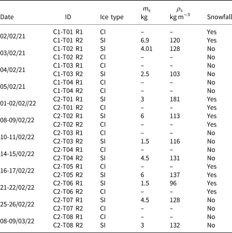
In the first campaign, 6.9, 4.0 and 2.5 kg of snow were added to the water, in experiments labelled C1T01, C1T02 and C1T03 respectively. In C1T04, CI formation was observed in both compartments. In the second campaign, the mass of snow submerged in water was 1.5, 3, 4.5 and 6 kg. An identical snow mass was tested twice (C2T01 to C2T08), but the snow was added to a different compartment each time, see Table 1.
Overall experimental matrix, including the time when the experiments were performed (dd/mm/yy), ID, ice type, snow mass, average snow density measured and snowfall occurrence during the experiment submerging in the water or accumulating on ice
Snow density was measured using a snow cutter of a volume of 0.25 L in several positions in the fresh snow on land. The fresh snow was collected from the top layer of snow and placed in plastic buckets to measure its mass. Subsequently, the snow was distributed in the water. It is recognised that this procedure of snow immersion may have affected the snow properties, such as snow density and porosity. It was observed that the snow maintained its loose texture throughout the procedure, however, the grain size and shapes of snow crystals were not investigated.
Ice thicknesses in both compartments were manually measured four times during each experiment. In addition to the temperature and thickness measurements, incoming light was also recorded during the second campaign using a Hukseflux pyranometer SR30-M2-D1 (ISO 9060:1990 standard) with a sensitive spectral range of 285–3000 nm.
At the end of each experiment, the ice was mechanically broken and removed to empty the tank, which was then topped up with water the night before the next experiment. For the next experiment the surface was cleared once again by removing the ice formed during the night and the water level was corrected to the level of 100 cm. Figure 1 illustrates the experimental setup.
Tank set up with front (left) and side views (right). The tank is divided into a congelation (CI) and a snow ice (SI) section. The blue short vertical lines illustrate the position of each thermocouple. The position of the pyranometer when measuring the incoming radiation and the reflected radiation from the different surfaces is also illustrated. Not to scale.

2.2 Temperature measurements
There are some differences in temperature measurements between the two experimental campaigns. In both campaigns, one thermocouple was placed 30 cm above the water level for air temperature measurements, and the second was mounted at the water's surface. In the first campaign, the third thermocouple was placed at a 30 mm depth and the fourth thermocouple was mounted at a depth of 80 mm, but in the second campaign the 3rd and 4th thermocouples were placed at depths of 50, and 900 mm, the last is assumed as the bottom of the tank.
In the first campaign (C1), the thermocouples were fixed along the wall of the tank and were angled to measure at a distance of 10 cm from the wall, but they were free-floating at the respective depths. Snow addition and possible water turbulences during the thickness measurements might have slightly displaced the thermocouples. In the second campaign (C2), the thermocouples were also fixed 10 cm from the wall, but with plastic plates attached to the side wall of the tank. As pointed out above, the ice formed in the tank was removed by mechanical breaking after each experiment. This process may have also displaced the vertical plates up to 15 mm below their initial positions.
The thermocouples were Type K wires connected to a TC-08 data logger and were monitored with PicoLog 6 software. Our thermocouples are classified as Tolerance Class 1, with an insulation rating between −75 and 260°C. The specified tolerance for class 1 thermocouples provided by the manufacturer is ±1.5°C. Details on sensor calibration are given in the supplementary material.
2.3 Thickness measurements
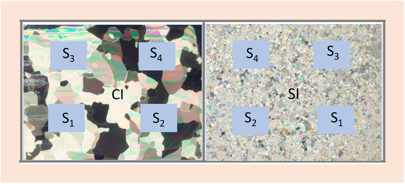
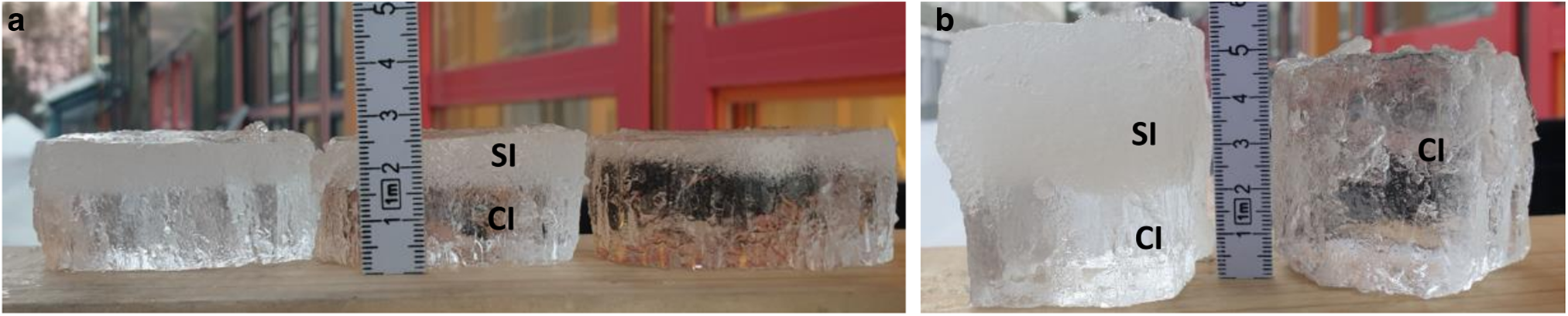
In the first campaign, the ice thickness in both compartments was measured every two hours, while in the second year, the thickness measurements was conducted after 6, 12, 24 and 30 h. The thickness measurements were conducted by drilling and sawing out several square ice pieces, each time at a different position. A schematic illustration of the sampling positions is given in Figure 2. The ice pieces were of different sizes for example up to 50 × 50 mm, see Figure 3. The thicknesses of the ice samples (SI & CI) were measured with a caliper. The slush underneath was merged with the SI, and it was possible to sample and measure its thickness. Lateral growth, up to 1 cm from the tank's walls was observed, however, the thickness measurements were carried out at least 10 cm from the walls.
The top view of the tank experiments and the four ice sampling positions (S 1, S 2, S 3 and S 4) in each compartment. The congelation ice (CI) and snow ice (SI) surfaces are distinguished by their common microstructure. Not to scale.
Examples of ice samples. (a) Three ice samples consisting of both congelation and snow ice; (b) the first sample consists of SI and CI underneath, while the second sample only of CI.
In all the SI experiments of the first campaign and the first experiment of the second campaign, the initial slush thickness (HSL0) which formed instantly after snow submergence was not measured. However, HSL 0 was calculated with an empirical regression equation that is detailed in Section 3. The construction of a small ruler with an angled protrusion at the end was suitable for measuring the initial slush thickness, in the seven following experiments. For this measurement, a small slush mass was carefully removed from the middle of the tank, and the ruler was used to determine the depth of the slush at the sides of the hole. Minor errors such as slush compression while measuring or not visually distinguishing the slush bottom when measuring may have occurred.
2.4 Radiation measurements
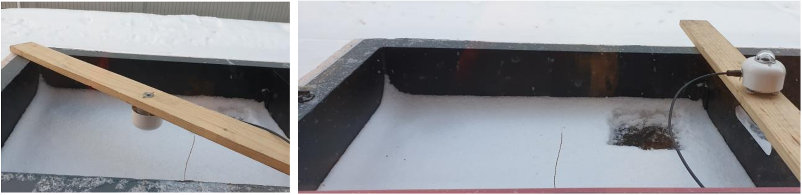
The pyranometer was placed between the two compartments, 20 cm above the water level, to continuously measure a representative value of the incoming solar radiation in both compartments, see Figure 4. The pyranometer was moved 3 to 5 times for a few minutes during the daylight to measure the outgoing radiation in both compartments 15 cm above the surface. Radiation measurements were calibrated considering the experimental setup. The detailed procedure for calibration is provided in the supplementary material. The albedo was calculated as the ratio between the measured incident and reflected radiation.
Top view of the second compartment during C2-T01 showing the pyranometer position when recording reflected radiation (left) and the pyrometer position between two compartments when recording the incident radiation (right).
3. Results
In this section, the results obtained by the temperature and thickness measurements in both campaigns as well as the radiation measurements from the second campaign are summarised.
3.1 CI and SI thicknesses
This section provides an overview of the measured thicknesses of congelation ice (HCI), snow ice (HSI) and slush (HSL) for all conducted experiments in both campaigns.
3.1.1 The first campaign (C1)
In the first three experiments, the slush layer was formed from the addition of 6.9, 4.0 and 2.5 kg of snow in T01R2, T02R1 and T03R2, respectively. During these experiments, only SI, and slush were present in the compartment where snow was submerged.
In T01, the CI and SI reached maximum thicknesses of 13 and 21 mm respectively, see Figure 5. The measured maximum thicknesses of CI and SI were 18 and 25 mm in T02 and 7.3- and 11.1-mm in T03. Referring to the total CI thickness, the HSI was 61.5, 38.9 and 54.8% higher than HCI, in T01, T02 and T03. During T01, snowfall occurred, and 5 mm of snow accumulated on the ice in both compartments. No snowfall occurred in the following experiments of C1.
Measured thicknesses of congelation ice, snow ice and slush (HCI, HSI and HSL) in the first campaign (C1). Figures a, b, c and d illustrate the results from the first, second, third and fourth experiments (T01, T02, T03, and T04), respectively. Snow was added only in one compartment (R1 or R2) in each of the first three experiments.

The slush thickness decreased with time as the SI thickness increased. However, in T02 and T03, there was a deviation from this trend. For example, the measured slush thicknesses after 6 h were higher than those after 4 h. This suggests that the initial slush layer was uneven due to manual snow distribution at the beginning of the experiment.
In T04 the growth of CI was investigated in both compartments. The maximum thickness of CI in each compartment was 10.5 and 11.9 mm, respectively. The variation in CI growth between compartments is attributed to the experimental error that may occur. In the initial ice formation phase, thickness measurements are more sensitive and prone to experimental errors compared to the later stages of ice growth (Toyota and others, Reference Toyota, Ono, Tanikawa, Wongpan and Nomura2020).
3.1.2 Second campaign (C2)
In the second campaign, the slush layer was created by adding 1.5 kg of snow in T03, and T06; 3 kg of snow in T01 and T08; 4.5 kg of snow in T04 and T07; and finally, 6 kg of snow in T02 and T05. During these experiments, CI formed beneath the SI due to the longer experiment duration. The total thickness of the initial SI and the CI formed underneath is represented as HT. The thickness results from C2 are given in Figs 6a–p.
Measured thicknesses of congelation ice (HCI), snow ice (HSI), slush (HSL) and snow (HS) in both compartments (R1 and R2) for all the experiments (from T01 to T08) carried out in the second campaign (C2). HT is the sum of HSI and HCI in the compartments where the total solid ice is comprised of both ice types. The amount of snow added to one of the compartments in each experiment is given in the title of each plot.

In the first experiment (T01), the slush transformed into SI within 6 h. After 30 h the total ice thickness (HT) was 8 mm thicker than CI. Snowfall occurred during the experiment, and the maximum thickness of snow accumulated on ice was 25 mm.
In T02, the initial slush layer had a thickness of 113 mm and formed a SI thickness equal to 36 mm. At the beginning of the experiment, a light snowfall occurred and contributed to slush formation in both compartments, but no dry snow accumulated on the ice. The total amount of incoming snow that was submerged in both compartments during the first 6 h was approximately 15 mm. This snowfall formed a 10 mm thick SI layer after 24 h, in the compartment where no snow was added. The ice thickness was 11 mm higher in the compartment where 6 kg was initially added.
In T03, an initial slush layer of 25 mm formed a SI thickness of 8 mm which remained unchanged after 12 h. HT was 5 mm higher than HCI. In T04, the 4.5 kg of snow submerged formed a 70 mm thick slush layer. This transformed to a 28 mm thick SI after 12 h. The difference in ice thickness between compartments was 7 mm, with maximum thicknesses of 63 and 56 mm, respectively.
In T05, 6 kg of snow formed a slush layer of 80 mm. Snow continued to fall throughout the experiment, leading to the formation of a SI layer in both compartments. After 30 h, a thick layer of dry snow (120 mm) accumulated on the ice. In the compartment where an initial snow mass was added, the slush layer did not freeze completely and SI reached a thickness of 19 mm, while the slush underneath was 8 mm thick. In the other compartment, the total ice thickness was 15 mm comprising both SI and CI.
In T06, 1.5 kg of snow formed a slush layer equal to 30 mm. The slush froze after 6 h and formed a 12 mm thick SI layer. The thickness difference between compartments was 4 mm. In T07, 4.5 kg of snow formed a slush layer equal to 75 mm which transformed completely to SI after 24 h. In T08, 3 kg of snow yielded a slush thickness of 40 mm, and the SI had a maximum thickness of 18 mm after 24 h.
After 24 and 30 h, the thicknesses of SI were 18 and 15 mm in T07R1 and 21 and 17 mm in T08R2. Even though the snow was distributed carefully in the water, the decrease of the SI thickness with time indicates an uneven initial slush layer. In addition to the mechanical distribution, the difference in the slush thickness and snow concentration was also a result of snow agglomeration when submerged into the water.
3.2 Temperature recordings
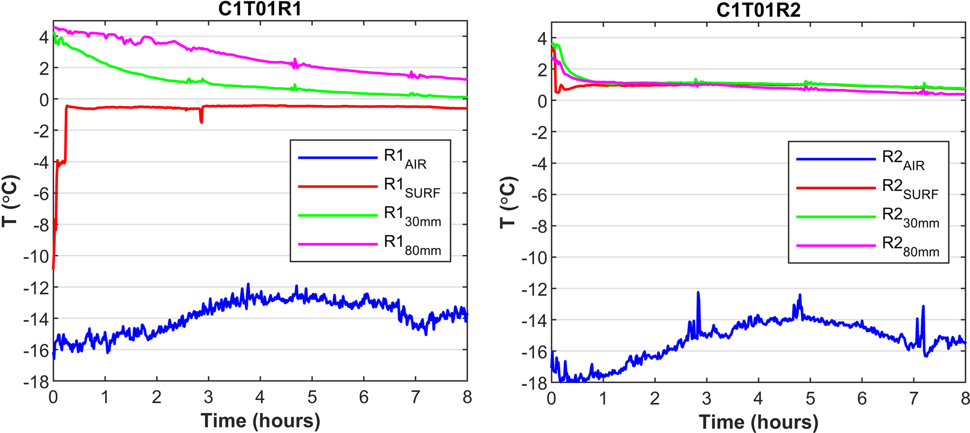
Examples from the continuous temperature recordings from both campaigns are given in Figs 7 and 8. During C1-T01-R1, the surface thermocouple initially measured the air temperature near the water surface, followed by the ice temperature see the red line in Figure 7. In C1-T01-R2, the temperature recordings on the surface and at depths of 30 and 80 mm remained above 0°C throughout the experiment and reached the similar values after approximately one hour. This indicates the displacement of the thermocouples beneath the slush layer or at the water/slush interface due to the snow addition. In the second compartment (R2), the surface thermocouple recorded a temperature peak some minutes after the start of the experiment, which indicated the cooling of water from snow submergence.
Continuous temperature readings during the first experiment of the first campaign. Congelation ice formation was investigated in the first compartment (R1), while in the second compartment (R2) 6.9 kg of snow was submerged in water. The blue, red, green and purple lines show the temperature recordings throughout the experiment, e.g., for the first compartment in the air (R1AIR), at the surface (R1SURF), at depths of 30 mm (R130mm) and 80 mm (R180mm).
Continuous temperature readings during the fifth experiment of the second campaign. Congelation ice formation was investigated in the first compartment (R1), while in the second compartment (R2) 6 kg of snow was submerged in the water. The blue, red, green and purple lines show the temperature recordings throughout the experiment, e.g., for the first compartment in the air (R1AIR), at the surface (R1SURF) and depths of 50 mm (R150mm) and 900 mm (R1BOT).

In the second campaign, the thermocouples were fixed in plastic plates, ensuring that the snow submergence did not displace them. This is evidenced by the negative temperatures recorded by the surface thermocouples. In the first compartment where no snow was added, the water surface reached the freezing point after approximately four hours, see Figure 8. Contrary to C2-T05-R2 the water cooling occurred instantly due to snow addition in the water.
Thermocouples at 50 mm depth recorded negative temperatures in all C2 experiments, even when the total CI thickness was below 50 mm. A possible explanation for this occurrence can be the displacement and freezing of the thermocouple tip. Therefore, the temperature recordings cannot be accurately correlated with the original depth of thermocouples. However, the air temperature recordings and the temperature difference between thermocouples are considered reliable in the current analysis.
3.3 Shortwave radiation
The incoming solar radiation recorded in the tank was compared with data recorded by the SMHI meteorological station at Luleå airport. Two examples of incoming solar radiation during T01 and T08 are illustrated in Figure 9. In T01 the radiation difference between SMHI and the tank recording was about 90 W m−2, while in T08 this difference reached up to 100 W m−2. This variation can be attributed to the tank's location between two buildings, which shaded the tank and limited its exposure to direct sunlight. As a result, the tank primarily received diffuse solar radiation.
Incoming solar radiation (φSW↓) measured at the SMHI meteorological station (airport Luleå) is indicated by the solid blue line and the solar radiation measured at the tank during the first and last experiments is shown by a solid red line. Midnight corresponds to t = 14 h.

Figure 10 illustrates the reflected radiation from the ice surfaces in both compartments for T01 and T08. In T01, at the beginning of the experiment, the reflected radiation measured in the first compartment was higher compared to the second compartment. This difference can be attributed to different surfaces: R1 had a surface consisting of slush, while R2 consisted of water. However, over time, snowfall accumulated on ice, and the reflected radiation resulted in almost similar values in both compartments. In T08, throughout the experiment, the reflected radiation from R2 was higher than that from R1. This difference was due to the SI formation in R1 while only CI was formed in R2.
The reflected solar radiation measured during the first and last experiments. The red and blue lines show the reflected radiation from the ice surface in the first and second compartments (R1 and R2), respectively. Midnight corresponds to t = 14 h. Note that the reflected radiation is similar in both snow-covered compartments in T01 after 4 h, while it is higher for bare snow ice (R2) compared to the bare congelation ice in T08R1.

Figure 11 illustrates the albedo calculated as the ratio of incident radiation to reflected radiation. An average albedo was calculated as the mean value of all measured daytime surface albedos (for incoming solar radiation higher than zero) during the 30 h of the experiments. This average value considers the albedo values from the beginning of the experiment when only slush or water was present until the end of the experiment when the ice was covered with snow. The reflected radiation illustrated in the first plot of Figure 10 from the 23rd to 27th hour corresponds to an average albedo of 0.83 in both compartments. This value is representative of snow-covered surfaces (Grenfell and Maykut, Reference Grenfell and Maykut1977; Perovich, Reference Perovich1996; Perovich and others, Reference Perovich, Tucbker and Ligett2002).
The albedo measured from the different compartments during the first (T01) and last (T08) experiments of C2. Note how the albedo of the bare snow ice in compartment R2 in the last experiment (T08) is visibly higher than the albedo of bare congelation ice in R1.

4. Snow-slush-snow ice transformation theory
This section outlines the theory, assumptions and model formulations pertaining to snow-slush-snow ice transformation, as used in this study.
4.1 Slush formation
Snow will completely submerge in water (unless it falls on ice and accumulates as dry snow). If the water surface temperature is uniform, and close to the freezing point, the natural snowfall into the water will form a slush layer. In this study, the snow was distributed by hand, so some horizontal variation of the slush thickness can be expected.
The initial slush thickness (HSL0) is governed by the initial amount of snow that is distributed in the water. The theoretical uniform snow thickness Hs evenly distributed on a dry surface equal to the compartment's surface area (AR = 0.585 m2) was estimated from the mass and density measurements as:

where ms is the snow mass, and ρs is the snow density, see Table 1.
It is assumed that Hs is the initial snow thickness submerged in water and all the air pores of snow are replaced with water. The air/snow fraction is then assumed to be equal to the water/ice fraction (Adolphs, Reference Adolphs1998), and the initial slush thickness (HSL0) equals HS (Eqn (1)). The porosities of snow and slush are considered equal, and the maximum slush density (ρslmax) can be calculated from:

where subscripts sl, s, w and i stand for slush, snow, water and ice. The density of fresh water ice (ρi) is 917 kg m−3 (Cox and Weeks, Reference Cox and Weeks1983).
When snow submerges in water, the ‘warm’ water, and the ‘cold’ snow exchange heat. In a closed system, the specific heat flux will approach zero when slush and water reach temperature equilibrium (e.g., Lei and others, Reference Lei2014). Depending on the heat content some slush may transform into water or SI. The fraction of ice that may melt or freeze can be estimated by considering mass and energy conservation balance within a closed system. This estimation assumes that the heat exchange between the submerged snow and water, until temperature equilibrium is reached, is not influenced by the simultaneous heat exchange at slush/atmosphere and slush/water interfaces. This assumption is valid when temperature equilibrium is reached quickly.
The net energy balance (E) between snow and water is equal to the sum of energy released from water cooling (Ew) and the energy consumed from warming the snow, Es. A positive E suggests that the excess energy goes into melting slush while a negative balance suggests the freezing of slush. The net energy balance is as follows:

where cw = 4217 J kg−1°C−1 (Incropera and others, Reference Incropera, Dewitt, Bergman and Lavine2007) and cs = 2117J kg−1°C−1 (Mellor, Reference Mellor1977) are the specific heat capacities of water and snow, respectively. If the slush equals the theoretical snow thickness, then the water thickness (HW) can also be considered equal to HS. (TW-TSL) and (TS-TSL) are the temperature gradients (ΔTW and ΔTS) between the initial water (TW) and snow (TS) temperatures with the slush temperature (TSL) in equilibrium. Snow temperature and air temperature are assumed to be equal.
After snow submersion in water, the excess energy will melt a fraction of the ice crystals, thus increasing the water content (porosity) in the slush layer and melting the slush at the water/slush interface. The deficiency of energy will increase the slush porosity by merging and freezing into SI. Presuming that the fraction of slush that melts and freezes in the pores equals a representative equivalent thickness change (ΔHSL), this is equal to:

where Li is the latent heat of ice formation (3.34.105 J kg−1). In the current study, ρslmax, and slush densities of 600, 700, 800 and 900 kg m−3 (Weeks and Lee, Reference Weeks and Lee1958) are used in estimating ΔHSL. Assuming that the slush porosity is equal to the snow porosity (psl = ps = 1–ρs/ρi) and the initial slush thickness (HSL) equals the theoretical HS, the instant slush porosity (ΔpSL) reduction or increase is:

The assumption that HSL 0 equals HS neglects possible instant occurrences such as crystal agglutination or separation. These processes may lead to instant snow compression or expansion, respectively.
In a companion study, 20 experiments were performed to investigate the initial thickness of slush that was formed from snow submergence in a transparent container (Zhaka and others, Reference Zhaka, Bridges, Riska and Cwirzen2022). This study statistically analysed the effect of the initial snow mass or theoretical thickness, initial snow temperature and water temperature in the slush thickness (HSL0) instantly after the submergence. A linear regression equation that determined the HSL 0 as a function of the theoretical HS was obtained (Zhaka and others, Reference Zhaka, Bridges, Riska and Cwirzen2022), and was used here to estimate the HSL 0 for the C1 series of experiments as well as C2T01.
4.2 Water and slush freezing
The ice growth is estimated from two simple models. The first model (Stefan, Reference Stefan1889) neglects the surface heat budget, the water heat flux, the snow layer and the thermal inertia. The air and ice surface temperatures are considered equal (TA = TS), and the ice growth equation is derived from the continuity equation at the ice/water interface. The ice thickness, H, is given by:

where Stefan's growth rate coefficient (a) in mm°C−0.5 −0.5 is

and the cumulative freezing air temperatures (θ in °C d) equates:

TF is the freezing temperature of fresh water (0°C).
The second model (Ashton, Reference Ashton1986, Reference Ashton1989) considers the heat exchange at the ice/atmosphere interface and the water heat flux (φw) at the ice/water interface. The ice growth model for CI is:

The value of the pure ice heat conductivity ki at the freezing temperature is assumed equal to 2.07 W m−1°C− (Yen, Reference Yen1981). The convective heat transfer coefficient hia (in W m−2 °C) at the ice/air interface is determined by fitting the model with all the measured thicknesses of CI.
The estimation of SI from freezing slush assumes a φw = 0 at the SI /slush interface. When estimating the CI formation under the SI the water heat flux is considered. The thickness of SI (HSI) for initial conditions of (HSI0 = 0) at t = 0 is:

The naturally formed slush has a density lower than ρslmax (Weeks and Lee, Reference Weeks and Lee1958), because the air pores present in the snow are partly replaced by water. Thus, the SI density (ρsi) is assumed equal to 900 kg m−3 (Ager, Reference Ager1962). SI with a bulk density equal to 900 kg m−3 has a snow-ice conductivity coefficient (ksi) equal to 2.03 W m−1 °C−1 (Schwerdtfecer, Reference Schwerdtfecer1963). The convective heat transfer coefficient in the snow-ice/air interface (hsia) is determined by the model fit with all the measured SI thicknesses. The SI growth equation assumes that the freezing takes place only in the water filled voids present in the slush layer. Assuming that the water fraction (vw) in the slush layer is equal to the air fraction (va) in dry snow than, vw is:

The analytical solution that considered the dry snow and the snow/atmosphere coupling effect adds in the above models (Eqns (9 and 10)) the equivalent heat transfer coefficient (he) from the snow layer to the atmosphere:

For a snow density ρs equal to 200 kg m−3, the snow thermal conductivity ks is equal to 0.1034 W m−1 °C−1 (Yen, Reference Yen1981). The convective heat transfer coefficient hsa at the snow/air interface differs from hia, which is the case when the snow layer is neglected.
In the current study, the thickness estimations were carried out considering: (1) all the CI measured from different experiments; (2) all SI measurements for the duration where only SI was freezing from slush; (3) all experiments where CI was formed under SI. The water heat flux was considered when estimating the CI thickness, but it was neglected when estimating the SI growth. The insulative effect of the slush layer underneath the freezing boundary was considered instead. Three different formulations for calculating the water heat flux are elaborated in the supplementary material: (1) where φw was estimated from the heat flux budget at the ice/water interface (Purdie and others, Reference Purdie, Langhorne, Leonard and Haskell2006; Lei and others, Reference Lei2014, Reference Lei2018); (2) the molecular conductivity earlier applied by Sengers and others (Reference Sengers, Watson, Basu, Kamgar-Parsi and Hendricks1984); and Ramires and others (Reference Ramires1995); (3) the parameterised equation earlier used in lake ice estimations (Shirasawa and others, Reference Shirasawa, Ingram and Hudier1997, Reference Shirasawa, Leppäranta, Kawamura, Ishikawa and Takatsuka2006; Ohata and others, Reference Ohata, Toyota and Shiraiwa2016). In the current data analysis, we used φw calculated from molecular conductivity formulation.
5. Data analysis
In the following subsections, the initial slush thickness and the phase transition in the slush/water interface are assessed. The thickness of SI formed from the initial slush thickness is also analysed. Furthermore, the freezing rate of slush is compared to the freezing rate of water and the CI growth under the SI layer is compared with CI growth under CI. The albedo differences between slush and water; and between SI and CI are presented.
5.1 Snow to slush transformation
The theoretical snow thicknesses (HS), the estimated initial slush thickness (HSL0e from Eqn (3)), and the measured initial slush thicknesses (HSL0m) introduced in Section 3 are summarised in Table 2. HSL0m are plotted against the theoretical snow thicknesses, see Figure 12. The linear regression equation (HSL0m vs HS) indicates that the snow expanded when submerged in water, the same behaviour was also reported earlier (Zhaka and others, Reference Zhaka, Bridges, Riska and Cwirzen2022).
Snow mass (ms), theoretical snow thicknesses (HS), estimated initial slush thickness (HSL0e) from Eqn (3), measured initial slush thicknesses (HSL0m), temperature differences (ΔTw) between initial TW and TSL at equilibrium, slush equivalent thickness (ΔHSL0) and porosity changes (Δpsl) at temperature equilibrium
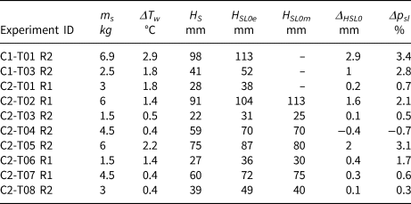
Measured initial slush thicknesses (HSL0) for seven experiments (C2T02 to C2T08) plotted against the theoretical snow thickness (HS). The regression dashed black line indicates that the snow expanded when submerged in water. The blue solid line shows HS vs HS (1:1 line).

The temperature gradient between the snow and water leads to the melting or freezing of slush in the water-filled pores as well as at the water/slush interface. This initial slush transformation was expressed in Section 3 as an equivalent thickness change ΔHSL (Eqn (5)), and slush porosity change ΔpSL (Eqn (6)). The ΔHSL and ΔpSL were calculated for different slush densities within the interval of 600 kg m−3 to ρslmax. The decrease of the slush density from its maximum to 600 kg m−3 increased the ΔHSL from 2.2 to 3.8 mm in C1T01. Also, the instant change of slush porosity increased when decreasing the ρsl. The ΔHSL and ΔpSL given in Table 2 are calculated for a slush density equal to 800 kg m−3. This density value was presumed a reasonable approximation considering the values reported in the literature between 600 and 850 kg m−3 (e.g., Weeks and Lee, Reference Weeks and Lee1958). These slush densities indicate that not all the air pores are replaced with water when snow submerges, but instead air pores remain in the slush (Colbeck, Reference Colbeck1997).
After the snow submersion, the surface thermocouples recorded a temperature decrease (ΔTw) of 2.9°C, and 1.8°C for C1T01 and C1T03, respectively. These ΔTw correspond to a porosity increase (ΔpSL) of 3.4 and 2.8%. In C1T02R1, the initial temperature decrease was not recorded due to a restart error of the temperature logger.
In the second campaign, the surface thermocouples recorded the temperature peak caused by snow submergence in all the experiments, except for T04. The ΔTw recorded at 50 mm depth is given instead in Table 2. The ΔTw after the snow submergence varied between 0.4 and 2.2°C in C2-T08 and C2-T05, corresponding to ΔpSL of 0.3 and 3.1%. In C2-T04, the results indicate SI formation and an instantaneous decrease in porosity of 0.7%. This decrease was caused by the low-temperature gradient (0.4°C) between the initial water temperature and equilibrium slush temperature, and a higher temperature gradient (12.4°C) between the initial snow temperature and the equilibrium slush temperature. The calculated values of ΔHSL are negligible compared to the measurement errors present in the initial slush thickness.
Theoretically, the instantaneous change in porosity until temperature equilibrium also occurs when SI forms in the other two mechanisms, in snow/ice interface flooding (Knight, Reference Knight1988) or the snow-ice formation initiated by precipitation. In these cases, the temperature difference between snow and seawater or precipitation water determines the occurrence of melting or freezing in the slush layer.
5.2 Initial phase transition at the slush/water interface
After the snow addition in the first campaign (C1), the surface thermocouples were submerged at the slush/water interface and recorded the temperature history at this interface. This provided qualitative insight regarding the heat exchange and phase transition between the snow, slush and water phases. The temperature recordings for the first 30 min of C1-T01 and C1-T03 (see Fig. 12) were interpreted based on the ice-water phase transition principles (Demirbas, Reference Demirbas2006).
The snow-slush-water initial transition underwent four main stages after snow submersion, see Figure 13a. The first stage was the temperature drop caused by the snow addition in the water, which lasted two minutes. The second stage was a period of constant temperature, during which the slush-water phase change occurred. This phase lasted four minutes and melted a slush equivalent thickness of 2.9 mm. In the 3rd stage, the interface layer reached the temperature equilibrium 4 min after the snow addition. In the last stage, the water temperature increased, due to the temperature difference between the bottom of the tank and the slush/water interface. This temperature increase suggests that the slush/water interface moved upwards as the slush melted or compressed with time due to buoyancy.
Temperature recordings at the slush/water interface for the first 30 min of C1T01R2 (a) and C1T03R2 (b).

During C1-T03, the snow addition was not instantaneous. Slower snow submersion in water caused a temperature fluctuation and elongated the first stage of the temperature drop, see Figure 13b. The phase change stage and the increase in the water temperature due to water heat flux cannot be precisely separated. These two phases are distinguished by the equilibrium temperature, which was reached instantly. The temperature equilibrium was reached instantly also in all C2 experiments.
5.3 Slush transformation to snow-ice
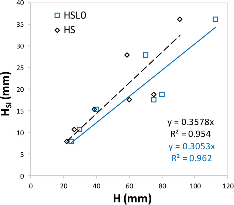
In the current study, only about 35% of the initial snow thickness or 30% of initial slush thickness transformed into SI, see Figure 14. The slush-snow ice transformation ratio (HSL0/HSI) was found to be 3.2 with a std dev. of 0.7. The regression equation given in Figure 14. can be used to estimate the thickness of SI based on the initial snow or slush thicknesses. Ice crystals are less dense than the water, consequently, the slush layer might be compressed under its own buoyancy, reducing its initial thickness and porosity. However, the extent to which the slush can compress and the duration of this process remain unclear.
The total snow ice thickness (HSI) formed in seven experiments (C2T02 to C2T08) is given as a function of the measured initial slush thickness (HSL0) and theoretical initial snow thickness (HS). The regression equations and goodness of fit for HSL0 vs HSI and HS vs HSI are given with blue and black font, respectively.
In the current experiments, the initial slush thickness is bounded by air and water and the phase change can take place at both boundaries simultaneously. Assuming that the slush is at freezing temperatures throughout, SI will initially form at the slush/air interface and will continue to grow downwards as heat is released into the atmosphere. At the same time, a water column with a positive temperature gradient will generate a water heat flux, which can melt the slush at the slush/water interface. The freezing and melting of slush at the upper and lower interfaces continue until the slush layer completely transforms into SI or is completely melted. Note that slush compression and melting might occur at the same time. However, from the current experiments, the compression rate due to buoyancy cannot be addressed and slush reduction with time is attributed only to the melting process. Therefore, about 70% of the slush melted due to water heat flux or compressed due to buoyancy.
Earlier studies of snow-ice formation in nature have reported different snow-slush-snow ice transformation ratios. For example, the transformation ratio of snow to slush in the snow/ice interface was 2/3 of the initial snow layer above the ice, and only half of the slush layer transformed to SI (Leppäranta and Kosloff, Reference Leppäranta and Kosloff2000), while elsewhere for the same mechanism, 1/3 of the initial snow layer on lake ice transformed to slush due to interface flooding (Knight, Reference Knight1988). Ohata and others (Reference Ohata, Toyota and Shiraiwa2016) showed that half of the maximum snow thickness over the ice transformed into SI.
5.4 Snow ice and congelation ice growth
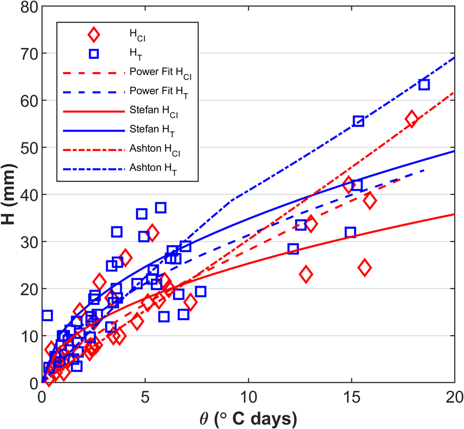
SI, slush and water were present in the SI experiments during the first campaign (C1), while in the second campaign (C2), CI began to form under the SI after approximately 12 h. The snow-ice and CI thicknesses (HSI and HCI) measured during C1 and the one measured during the first 12 h of each experiment in C2 are plotted against the cumulative freezing air temperatures (θ in °C d) in Figure 15. This figure shows the best power trendline fit, Stefan's (Reference Stefan1898) and Ashton's (Reference Ashton1989) models (see Section 3 Eqns (6, 9 and 10)). The scatter in thicknesses was mainly a result of uncontrolled environmental conditions.
The measured and estimated thicknesses of congelation (CI) and snow ice (SI) are plotted against the cumulative freezing air temperatures (θ). The measured thicknesses of congelation ice (HCI) and snow ice (HSI) in the first campaign (C1) and the first 12 hours of the second campaign (C2) are given with red diamonds and blue squares, respectively. The best power trendline fits for both CI and SI are given with dashed red and blue lines. The estimated thicknesses of CI and SI from Stefan's (Reference Stefan1889) Eqns (15 and 16) are illustrated with solid red and blue lines, while Ashton's (Reference Ashton1989) model fits (Eqns (9 and 10)) are illustrated with dotted red and blue lines for CI and SI respectively.

The power regression equation that fits best the measured SI and CI thicknesses are (see Fig. 15):


These trendlines showed a difference of 6 mm between HSI and HCI for a θ equal to 7°C d. The correlation coefficients were equal to 0.78 and 0.76 in Eqns (13 and 14), respectively. The power exponent in the snow-ice formation (0.51) is closer to the one proposed by Stefan (Reference Stefan1889) for the ice growth (0.5). The exponent that best fits the CI thickness measurements is larger (0.74). This is close to the exponent given by Ashton's (Reference Ashton1989) ice growth formulation. These exponents suggest that the SI growth rate decreased quicker with increasing θ compared to CI.
Fitting Stefan's (Reference Stefan1889) ice growth formulation results in the following equations:


where the values 6 and 10 are Stefan's ice growth rate coefficient in mm°C−0.5 d−0.5 (Eqn (7)). Based on this formulation the SI grew 4 mm faster than the CI, and for a maximum θ equal to 7°C d the SI was 10 mm higher than CI.
The estimation of CI growth with Ashton's (Reference Ashton1989) Eqn (9) included a water heat flux term but was neglected when estimating the SI growth. The CI thickness was estimated using the maximum water heat flux estimated from all the experiments, which varied between 72 and 2.4 W m−2. Ashton's (Reference Ashton1989) ice growth formulation gave the best fit for SI and CI thicknesses when air/ice heat convective coefficients were 16 and 18 W m−2 °C−1. This difference between hi and hsi suggests that higher heat is conducted through the CI than the SI, which is attributed to the water heat flux term added in the HCI. When the water heat flux term is omitted from Ashton's model then hi equals 13 W m−2 °C−1.
5.4.1 Total thickness (SI + CI)
For the second campaign (C2), the total thickness (HT) represents the initial SI thickness formed from freezing all the slush within the first 12 h, and thereafter it is the sum of the SI and CI thickness formed underneath it. Figure 16 shows all the ice thickness measurements including the snow-covered and bare ice, together with the best power trendline fit, and Stefan's (Reference Stefan1889) and Ashton's (Reference Ashton1989) model fits.
The measured and estimated congelation ice (HCI) and total ice thicknesses and (HT) are plotted against the cumulative freezing air temperatures (θ). The measured thicknesses of congelation ice (HCI) and total thicknesses of the snow ice experiments (HT) of the second campaign (C2) are given with red diamonds and blue squares. The best power trendline fits for both HCI and HT are given with dashed red and blue lines. The estimated HCI and HT with Stefan's (Reference Stefan1889) model is illustrated with solid red and blue lines, while Ashton's (Reference Ashton1989) model fits are illustrated with dotted red and blue lines.
Stefan's (Reference Stefan1889) equation gave a growth rate coefficient equal to 8 and 11 mm°C−0.5 d−0.5 for HCI and HT, respectively. For θ equal to 18°C d the difference between HCI and HT reached up to 13 mm. The reduction in the growth rate by 1 mm when comparing HCI with HSI and HCI with HT may indicate that CI under CI forms faster than CI under SI.
Also, the best-power fit equation for HCI crosses the equation for HT at approximately 17°C d. This suggests that initially the SI + CI had a higher thickness due to the quick initial growth of SI, but when HSL = 0, the CI growth under CI was slightly quicker than the CI growth under SI. It is probable that after HCI equals the HT (SI + CI), the HCI exceeds the HT. The current results are limited only to the number of cumulative air freezing temperatures where HCI approached HT but did not exceed it.
When estimating HT, the water heat flux (φw) was assumed zero during SI growth and between 37 and 2.4 W m−2 when CI formed under SI (from the maximum calculated water heat flux). The addition of φw after t = 12 h and θ = 9°C d (when estimating CI growth under SI) changes the slope in Ashton's model, see Figure 16. The ice growth models gave the best fit for HT and HCI using the air/ice heat convective coefficients (hi) equal to 17 and 18 W m−2 °C−1. As expected, the heat transfer coefficient in this case of HT is the average value between the one estimated for SI and CI, see Figure 15.
5.4.2 Snow-covered ice
Figure 17 illustrates the measured snow-covered ice thicknesses (HCI and HT). The power trendline fits for HCI and HT have almost similar power exponents close to 0.6 and a difference in the growth rate coefficient equal to 1 mm°C−0.5 d−0.5, see the power equations given in Figure 17. Stefan's (Reference Stefan1989) growth model fits both snow-covered thicknesses HCI and HT for a growth rate coefficient equal to 8 mm°C−0.5 d−0.5. Ashton's (Reference Ashton1989) model fits all the snow-covered thicknesses (HCI and HT) for the same snow/air convective heat transfer coefficient (hs) of 30 W m−2 °C−1. The snow/air convective heat transfer coefficient results were considerably higher than the convective heat transfer coefficients at the CI/air and SI/air interfaces (18 and 16 W m−2 °C−1).
The measured and estimated thicknesses of snow-covered congelation ice (HCIs) and snow-covered CI + SI (HTs) are plotted against the cumulative freezing air temperatures (θ). The snow-covered CI and CI + SI thicknesses are illustrated with red diamonds and blue squares. The dashed red and blue lines illustrated the best power trendline fit with the measured values. Stefan's (Reference Stefan1898) and Ashton's (Reference Ashton1989) model fits are illustrated with a solid and dotted cyan lines, respectively. Note that the same model lines fit all snow-covered thicknesses (HCI and HT).

5.5 Congelation ice growth under snow ice
The rate of water freezing under a SI layer is being compared to the rate of water freezing under a CI layer. The thickness of the CI (ΔHCI) formed under the existing CI layer in a time interval Δt is equal to H CI (t + Δt) – H CI (t), where t is the time of measurement. The CI thickness (ΔHCIs) formed under the existing SI layer is equal to H CIs (t + Δt) – H Cis (t), for the same time interval (Δt) as the CI measurements. These thickness differences are plotted against the difference in cumulative air freezing temperatures (Δθ = θ(t + Δt) – θ(t)) for the same time interval (Δt), as shown in Figure 18. Even though the data of ΔHCIs vs Δθ include scatter, the linear regression equation fitted on the data illustrates that the difference between water freezing under CI and SI is small. Considering the power equation fit (ΔHCIs vs Δθ), the coefficient of growth rate between the CI growth under CI and SI differs with 1 mm°C−0.5 d−0.5. Also, the Stefan model fit in Figure 16 indicated that CI growth under SI was slightly lower compared to CI growth under CI.
The measured thicknesses of the congelation ice (ΔHCI) formed under the existing CI layer and the SI layer (ΔHCIS) in a time interval Δt and plotted against the cumulative freezing air temperatures (Δθ) for the same time interval (red diamonds and blue squares respectively). The best linear and power trendline fits are also illustrated with dashed and dotted red and blue lines for ΔHCI and ΔHCIS, respectively.

5.6 Solar radiation
A representative albedo value for open water is 0.06. It is 0.52 for bare first-year ice, and for melting white ice the albedo may range between 0.56 and 0.68 (Perovich, Reference Perovich1996). A representative albedo value for refrozen white ice is 0.7 (Allison and others, Reference Allison, Brandt and Warren1993; Perovich, Reference Perovich1996). In the current study, the albedo measured in each compartment in the time interval of 0.2 to 3.3 h for open water/thin CI varied between 0.047 and 0.147 with an average of 0.09, see Figure 19a. The albedo of slush/slush-thin SI varied between 0.1 and 0.2 with an average of 0.15. These albedo values are the averages of the initial phase of formation without distinguishing between the albedo of water and thin ice or between slush and SI. The albedo difference between the bare ice surface of SI and CI (Δa = aSI – aCI) resulted in a positive albedo difference and increased with the increase the initial snow mass, as shown in Figure 19b.
(a) Measured albedos at the beginning of each experiment. The blue bars illustrate the open water or thin congelation ice (CI) albedos, while the patterned light blue bars show the slush surface or thin snow ice (SI) albedos. (b) The difference in average albedo (Δa) between SI and CI in T02, T03, T04 and T08 vs the initial snow mass submerged in water.

The radiation heat flux absorbed or scattered by the total ice thickness for 30 h was simply determined from the extinction law of radiation considering extinction coefficient earlier presented by (Arndt and others, Reference Arndt2017) and radiation penetration coefficient after (Sahlberg, Reference Sahlberg1988). On average, the amount of radiation that remained on ice varied between 0.6 to 2 W m−2. Despite the higher albedo of SI compared to CI, the amount of radiation that was absorbed or scattered from the total ice thickness was slightly greater for HT (SI + CI) compared to HCI. This was a result of the higher thicknesses of (SI + CI) compared to the CI. For example, in the last experiment (C2T08), the CI had on average absorbed 0.83 W m−2 of solar radiation which corresponds to a temperature increase of 0.03°C. While in the other compartment where snow was submerged, the SI + CI had in average absorbed 1.14 W m−2 which correspond to an ice temperature increase of 0.034°C.
6. Discussion
When the snow was submerged in water, the temperature equilibrium was reached instantly, and the slush phase change in the water-filled pores and at the slush/water interface occurred instantly. A similar result was also reported in a saline slush formation laboratory study (Jutras and others, Reference Jutras2016). The initial slush thickness was found to be higher than the calculated submerged thickness, suggesting that snow expands when submerged in water close to the freezing point. This observation was also made earlier by Zhaka and others (Reference Zhaka, Bridges, Riska and Cwirzen2022).
If all the slush transforms to SI, then the total thickness (slush + snow ice) should remain constant over time. However, in the current experiments, the total thickness decreased with time. This decrease may be attributed to the compression of slush over time due to the buoyancy force, resulting in a reduction in both slush porosity and thickness. Additionally, slush melted at the water/slush interface due to water heat flux. It is possible that both phenomena occur simultaneously. However, in the current study, these phenomena cannot be distinguished.
A significant distinction between the SI formation observed in the current study and the SI formation resulting from level ice flooding is the presence of different boundary layers in the top and bottom of the slush. In the current experiments, the slush is initially bounded by air and water, whereas during SI formation due to flooding, the slush is bounded by dry snow or air and ice. This disparity in boundary conditions could explain the varying fractions of slush-to-snow ice transformation observed: approximately 0.3 in the present experiments vs 0.5 for SI formation by flooding (Leppäranta and Kosloff, Reference Leppäranta and Kosloff2000). Therefore, according to Figure 14 in the current study, it is evident that only about 30% of the initial slush thickness transformed into slush, and approximately 70% of the slush either melted due to water heat flux or compressed due to buoyancy.
The simple linear regression equations, illustrated in Figs 12 and 14, quantify the snow-slush-snow ice transformation. The first equation can estimate the initial slush thickness based on the theoretical snow thickness, and the second equation can estimate the total snow-ice thickness from the initial slush thickness. Both correlations can be used to estimate the SI formation by the first mechanism, where the SI forms from snowfall in freezing water in the early winter. Additionally, these simple equations can be used to evaluate the snow contribution to the total brash ice thickness formed in ship channels or ports.
For the same environmental conditions, it was observed the initial formation of SI from freezing slush was quicker than the initial ice growth from freezing water (CI). Stefan's model gave a growth rate difference between SI and CI equal to 4 mm°C−0.5 d−0.5. The quicker formation of SI compared to CI, can be attributed to several phenomena: (1) the slush only freezes in the water pores; (2) the temperature gradient in the slush layer is theoretically zero and (3) less solar radiation reaches the snow ice-water system due to a higher surface albedo of the SI compared to CI.
Thus, the slush beneath the freezing boundary (SI/slush) acts as insulation, preventing direct contact between the warm water and the freezing interface. In contrast, in the case of CI formation, the water is in direct contact with the freezing interface and provides heat, which can reduce or sometimes prevent the ice growth. During SI formation from slush, the water's heat flux melts the bottom of the slush layer. This explains why only about 30% of the initial slush layer transformed into slush.
Additionally, the albedo measured in open water/thin CI gave an average value of 0.09, while the albedo of slush/slush-thin SI averaged 0.15. The albedo difference between SI and CI was up to 0.12 (higher in SI). This albedo difference increased with increasing the mass of snow submerged in the water. This difference suggests that, for the same solar radiation intensity, the heat transmitted in CI/water interface is higher compared to the energy transmitted in the SI/slush interface.
However, the growth of CI under SI was slightly slower compared to CI growth under CI. The difference in the growth rate coefficient was estimated to be 1 mm°C−0.5 d−0.5 for a cumulative freezing air temperature of 9 °C d. This minor difference can be attributed to the varying conductive heat coefficients for the CI and SI. The presence of air pores within the SI lowers its conductivity from 2.07 W m−1°C−1 for pure ice with a density of 917 kg m−3 (Yen, Reference Yen1981) to 2.03 W m−1°C−1 for SI with a density as high as 900 kg m−3 (Schwerdtfecer, Reference Schwerdtfecer1963).
Despite the higher albedo of SI compared to CI, which may have affected the initial growth of SI, the absorbed radiation heat by the SI was higher compared to CI due to the thicker SI layer. This may have influenced the CI growth underneath SI and CI. However, a previous study of the thin ice growth initiated by snow submersion in the water suggested that the thickness of the SI layer did not significantly affect the subsequent ice growth rate (Toyota and others, Reference Toyota, Ono, Tanikawa, Wongpan and Nomura2020).
The estimated snow-ice growth rate in this study may have relevance for other snow-ice formation conditions and different mechanisms, such as the snow-slush-snow ice transformation that occurs in level ice from flooding and the transformation that is initiated by precipitation. In these cases, the slush is bounded by snow or air and by ice, which acts as insulation, protecting the slush from the water heat flux, while SI forms at the air/slush or snow/slush interfaces.
In the current study, the SI also formed at the air/slush boundary, and in a few experiments, snowfall also affected the ice growth. The slush beneath acted as insulation, protecting the SI from the water heat flux. This mechanism of slush transformation where the growth occurs at SI/slush interface while slush simultaneously melts at the slush/water interface, can be considered comparable to another process observed in drifting and coastal ice (Lytle and Ackley, Reference Lytle and Ackley2001; Shirasawa and others, Reference Shirasawa2005), where the slush to SI transformation occurred simultaneously with the bottom melting of CI.
Conclusions
Congelation and snow-ice growth experiments were carried out in a fresh water tank exposed to the outdoor freezing temperatures at Luleå University of Technology facilities in Sweden, during two consecutive winters in 2021 and 2022. This study investigated the snow-slush-snow ice transformation. The initial snow-ice (SI) growth from freezing slush was compared with the CI growth from freezing water. The tank was divided into two compartments to conduct simultaneous experiments. In each experiment, in one compartment the snow-slush-snow ice transformation was observed and in the adjacent compartment water freezing was investigated. The first campaign consisted of four experiments, each lasting 8 h. In the second campaign, eight experiments were conducted, each lasting 30 h.
About 30% of the initial slush layer transformed into SI and about 70% either melted or compressed due to the buoyancy. This fraction can be considered when estimating the SI formation at the beginning of winter when the snowfall submerges in the water close to the freezing temperatures. These findings can be used to assess the significance of the snow-slush-snow ice transformation in determining the overall thickness of brash ice formed in ports and ship channels.
The SI growth from slush was 4 mm °C−0.5 d−0.5 faster compared to CI growth from water. This can be attributed to three main factors. Firstly, the slush freezes only in the pores, which accelerates the freezing process. Secondly, the slush layer acts as an insulator, preventing the direct contact of SI with water. Additionally, the higher albedo of SI compared to CI (an average difference of 0.12) results in lower absorption of solar radiation, leading to reduced energy gain.
However, CI growth under CI was 1 mm °C−0.5 d−05 faster than CI growth under SI. This slight difference can be attributed to two factors. Firstly, the SI layer has a higher air content, which reduces the conductivity of SI compared to CI. Secondly, the initial thickness of SI is higher, resulting in slightly more solar energy absorption compared to CI.
This experimental setup provides an opportunity to further investigate and gain insights into the porosity and density transformation of snow-slush-snow ice, as well as these key parameters impact the thermodynamic properties and growth of SI in comparison with CI. Additionally, the same setup can be used to study the formation of SI resulting from flooding and melting processes.
Supplementary material
The supplementary material for this article can be found at https://doi.org/10.1017/aog.2023.58.
Acknowledgement
The authors would like to acknowledge the support from TotalEnergies, and the help received from the technicians and staff at the Luleå University of Technology.
Author contributions
VZh: Conceptualisation, planning the experiments, performing the experiment, data curation, data analysis, visualisation, writing the original manuscript, writing review and editing. RB: Conceptualisation, planning the experiments, performing the experiment, writing review and editing. KR: Conceptualisation, supervision, writing review and editing. AH: Hardware contributions, writing review and editing. AC: Conceptualisation, Supervision.


 Open access