


1. Introduction
Multiphase turbulent flows, where gases and liquids mix, are ubiquitous in industrial processes and natural phenomena. In applications ranging from chemical reactors and oil–gas pipelines (Delnoij et al. Reference Delnoij, Kuipers, van Swaaij and Akker1997) to oceanic wave breaking (Deane & Stokes Reference Diaz, Gonzalez and Vera2002), the interaction of bubbles with turbulence critically affects mass transfer, reaction rates (Clift, Grace & Weber Reference Crialesi-Esposito, Chibbaro and Brandt2005) and flow behaviour. For example, the coalescence and breakup of bubbles in turbulence governs interfacial area and influences efficiency in systems like emulsifiers, heat exchangers and wastewater aeration tanks (Coulaloglou & Tavlarides Reference Nambiar, Kumar and Gandhi1977; Martínez-Bazán et al. Reference Monin and Yaglom1999). High-Reynolds-number bubbly flows are especially important in devices such as multiphase pumps, where intense turbulence is deliberately generated to disperse gas into liquid (Javadi, Kumar & Aidun Reference Kantarci, Borak and Ulgen2026). In such pump operations, bubbles can significantly alter performance: their formation, coalescence and breakup can enhance mixing, but also cause loss of efficiency if not controlled (Kolmogorov Reference Kolmogorov1949; Hinze Reference Hosokawa and Tomiyama1955; Javadi et al. Reference Kantarci, Borak and Ulgen2026). For instance, in a multiphase pump impeller, strong turbulence fragments bubbles into smaller bubbles and influences the downstream two-phase flow (Zhang et al. Reference Zhang, Li, Vafai and Zhang2018). Given the prevalence of bubbles in turbulence in engineering (e.g. bubble columns, pipelines, nuclear coolant loops) and in natural phenomena (e.g. breaking waves, volcanic eruptions), understanding coalescence/breakup dynamics under extreme turbulence is both fundamentally and practically important (Liao & Lucas Reference Liberzon2009, Reference Loitsyanskii2010).
Quantifying the bubble size distribution is essential because it determines how bubbles partition across small and large sizes. A modified Gaussian function is commonly used, since it locates the most probable size, bounds the upper tail (e.g. $d_{\text{max}}$
) and measures the spread about the mean. These statistics are critical in systems such as (i) chemical bubble and slurry reactors (Kulkarni Reference Kumar, Quintero, Baldygin, Molina, Willers and Waghmare2007), (ii) bioreactors and wastewater aeration (Kantarci, Borak & Ulgen Reference Kim and Park2005; Garcia-Ochoa & Gomez Reference Garcia-Ochoa and Gomez2009), (iii) mineral flotation and dissolved air flotation processes (Wang et al. Reference Wang, Yang, Yan, Wang, Wang and Zhang2020), and (iv) CO
$d_{\text{max}}$
) and measures the spread about the mean. These statistics are critical in systems such as (i) chemical bubble and slurry reactors (Kulkarni Reference Kumar, Quintero, Baldygin, Molina, Willers and Waghmare2007), (ii) bioreactors and wastewater aeration (Kantarci, Borak & Ulgen Reference Kim and Park2005; Garcia-Ochoa & Gomez Reference Garcia-Ochoa and Gomez2009), (iii) mineral flotation and dissolved air flotation processes (Wang et al. Reference Wang, Yang, Yan, Wang, Wang and Zhang2020), and (iv) CO $_2$
absorption and scrubbing (Chen et al. Reference Chieco and Durian2023). The bubble size distribution strongly influences process behaviour. It controls mass-transfer layers and current stability in electrochemical systems (Taqieddin et al. Reference Taylor2017; Angulo et al. Reference Angulo, van der, Peter, Han and Rivas2020), delays slug formation and regulates pressure drop in gas-lift risers and pipelines (De Temmerman et al. Reference Delnoij, Kuipers, van Swaaij and Akker2015; Diaz, Gonzalez & Vera Reference Doherty, Ngan, Monty and Chong2024), and enhances near-wall renewal in membrane air scouring at fixed aeration power (Fabre & Liné Reference Friedlander1992; Alameedy et al. Reference Alameedy, Al-Sarkhi and Abdul-Majeed2025). In practice, the ratio between extreme and mean sizes becomes particularly informative: lower ratios stabilise current density and reduce electrode coverage by large bubbles, while bounding this ratio in pipelines helps maintain bubbly or churn flow and delays slug initiation (De Temmerman et al. 2015; Kumar et al. Reference Laakkonen, Moilanen and Aittamaa2023; Diaz et al. Reference Doherty, Ngan, Monty and Chong2024). In membrane systems, tuning this ratio increases renewal at the wall without promoting excessive fouling (Fabre & Liné Reference Friedlander1992; Alameedy et al. Reference Alameedy, Al-Sarkhi and Abdul-Majeed2025).
$_2$
absorption and scrubbing (Chen et al. Reference Chieco and Durian2023). The bubble size distribution strongly influences process behaviour. It controls mass-transfer layers and current stability in electrochemical systems (Taqieddin et al. Reference Taylor2017; Angulo et al. Reference Angulo, van der, Peter, Han and Rivas2020), delays slug formation and regulates pressure drop in gas-lift risers and pipelines (De Temmerman et al. Reference Delnoij, Kuipers, van Swaaij and Akker2015; Diaz, Gonzalez & Vera Reference Doherty, Ngan, Monty and Chong2024), and enhances near-wall renewal in membrane air scouring at fixed aeration power (Fabre & Liné Reference Friedlander1992; Alameedy et al. Reference Alameedy, Al-Sarkhi and Abdul-Majeed2025). In practice, the ratio between extreme and mean sizes becomes particularly informative: lower ratios stabilise current density and reduce electrode coverage by large bubbles, while bounding this ratio in pipelines helps maintain bubbly or churn flow and delays slug initiation (De Temmerman et al. 2015; Kumar et al. Reference Laakkonen, Moilanen and Aittamaa2023; Diaz et al. Reference Doherty, Ngan, Monty and Chong2024). In membrane systems, tuning this ratio increases renewal at the wall without promoting excessive fouling (Fabre & Liné Reference Friedlander1992; Alameedy et al. Reference Alameedy, Al-Sarkhi and Abdul-Majeed2025).
The bubble size distribution mainly depends on two factors: coalescence and breakup in the turbulent flow. Numerically, the bubble size distribution is obtained by solving a population-balance equation coupled to the turbulent flow field, where coalescence and breakup kernels, formulated from theoretical models and closed empirically, govern the redistribution of bubbles across sizes in space and time (Lehr, Millies & Mewes Reference Li, Liu, Xu and Li2002). These mechanisms have been extensively studied theoretically and computationally in turbulent environments, where energy dissipation, inertial forces and interfacial dynamics dictate the evolution of the bubble size distribution (Li & Liao Reference Liao and Lucas2024; Li et al. Reference Liao and Lucas2024). Bubble breakup in turbulence arises when inertial stresses exceed surface tension, fragmenting bubbles above a critical Weber number ( ${We}_{\textit{crit}}$
) (Kolmogorov Reference Kolmogorov1949; Hinze Reference Hosokawa and Tomiyama1955; Ni Reference Obukhov2024). The turbulence-based definition of the bubble Weber number is directly linked to the Kolmogorov description of breakup:
${We}_{\textit{crit}}$
) (Kolmogorov Reference Kolmogorov1949; Hinze Reference Hosokawa and Tomiyama1955; Ni Reference Obukhov2024). The turbulence-based definition of the bubble Weber number is directly linked to the Kolmogorov description of breakup:
 \begin{equation} {We} = 2.13\,\frac {\rho _\ell }{\gamma }\,(\varepsilon d)^{2/3}\,d. \end{equation}
Here $d$
is the bubble diameter,
$d$
is the bubble diameter, $\varepsilon$
is the turbulent energy dissipation rate per unit mass,
$\varepsilon$
is the turbulent energy dissipation rate per unit mass, $\gamma$
is the interfacial tension and
$\gamma$
is the interfacial tension and $\rho _\ell$
is the density of the continuous phase (Salibindla et al. Reference Sciacchitano and Wieneke2020). The Weber number corresponding to the maximum bubble size under given flow conditions is defined as the critical Weber number,
$\rho _\ell$
is the density of the continuous phase (Salibindla et al. Reference Sciacchitano and Wieneke2020). The Weber number corresponding to the maximum bubble size under given flow conditions is defined as the critical Weber number, ${We}_{\textit{crit}}$
, and the corresponding bubble diameter (
${We}_{\textit{crit}}$
, and the corresponding bubble diameter ( $d$
) is defined as the Hinze-scale diameter (
$d$
) is defined as the Hinze-scale diameter ( $d_{\textit{H}}$
) (Hinze Reference Hosokawa and Tomiyama1955; Hesketh, Etchells & Russell Reference Hibiki and Ishii1987). Experiments by Martínez-Bazán et al. (Reference Monin and Yaglom1999) showed a two-regime breakup frequency: rising near the critical size and decreasing for very large bubbles. Na, Chang & Lim (Reference Ni2022) reported a turbulence-driven power-law size distribution in oceanic flows. Direct numerical simulation (DNS) studies revealed further detail: Vela-Martín & Avila (Reference Vela-Martín and Avila2022) demonstrated memoryless breakup even for sub-Hinze droplets, while Calado & Balaras (Reference Chan, Dodd, Johnson, Urzay and Moin2024) highlighted enhanced deformation when bubble size matches energy-containing eddies. Models by Prince & Blanch (Reference Prince and Blanch1990), the energy cascade framework by Nambiar & Gandhi (Reference De Temmerman, Maere, Temmink, Zwijnenburg and Nopens1990), and Li & Liao (Reference Liao and Lucas2024)’s turbulence modulated breakup relate breakup rates to turbulent dissipation and deformation. High Reynolds numbers amplify breakup via increased shear and energy cascade to small scales (Sajjadi et al. Reference Scarbolo, Bianco and Soldati2013; Chen et al. Reference Chesters2021), making the Weber number central to predicting fragmentation (Li & Liao Reference Liao and Lucas2024), with bulk-phase dissipation further modulating breakup dynamics (Nguyen et al. Reference Obukhov2013).
$d_{\textit{H}}$
) (Hinze Reference Hosokawa and Tomiyama1955; Hesketh, Etchells & Russell Reference Hibiki and Ishii1987). Experiments by Martínez-Bazán et al. (Reference Monin and Yaglom1999) showed a two-regime breakup frequency: rising near the critical size and decreasing for very large bubbles. Na, Chang & Lim (Reference Ni2022) reported a turbulence-driven power-law size distribution in oceanic flows. Direct numerical simulation (DNS) studies revealed further detail: Vela-Martín & Avila (Reference Vela-Martín and Avila2022) demonstrated memoryless breakup even for sub-Hinze droplets, while Calado & Balaras (Reference Chan, Dodd, Johnson, Urzay and Moin2024) highlighted enhanced deformation when bubble size matches energy-containing eddies. Models by Prince & Blanch (Reference Prince and Blanch1990), the energy cascade framework by Nambiar & Gandhi (Reference De Temmerman, Maere, Temmink, Zwijnenburg and Nopens1990), and Li & Liao (Reference Liao and Lucas2024)’s turbulence modulated breakup relate breakup rates to turbulent dissipation and deformation. High Reynolds numbers amplify breakup via increased shear and energy cascade to small scales (Sajjadi et al. Reference Scarbolo, Bianco and Soldati2013; Chen et al. Reference Chesters2021), making the Weber number central to predicting fragmentation (Li & Liao Reference Liao and Lucas2024), with bulk-phase dissipation further modulating breakup dynamics (Nguyen et al. Reference Obukhov2013).
Bubble coalescence in turbulent flows is governed primarily by collision frequency and coalescence efficiency (Scarbolo, Bianco & Soldati Reference Seal, Das and Sen2015). Early foundational models, such as Coulaloglou & Tavlarides (Reference Nambiar, Kumar and Gandhi1977), introduced population-balance frameworks based on turbulent eddy collisions and liquid-film drainage mechanisms, establishing a fundamental framework for modelling bubble coalescence. Guo et al. (Reference Hesketh, Etchells and Russell2016) and Prince & Blanch (Reference Prince and Blanch1990) further developed this approach by distinguishing between collision frequency and coalescence efficiency, explicitly incorporating turbulence, buoyancy and viscous shear effects into their coalescence kernel. The Luo & Svendsen (Reference Matiazzo, Decker, Bastos, Silva and Meier1996) model refines these approaches by explicitly incorporating turbulence dissipation scales into predictions of collision and coalescence efficiency through film drainage modelling, proving especially effective at high void fractions (Nambiar & Gandhi Reference De Temmerman, Maere, Temmink, Zwijnenburg and Nopens1990; Luo & Svendsen Reference Matiazzo, Decker, Bastos, Silva and Meier1996). The recently developed interfacial area transport equation (IATE) further categorises coalescence events into random collisions, wake-entrainment events and hydrodynamic instabilities, offering a comprehensive framework widely accepted for detailed analyses of bubble interactions (Kamp, Chesters & Colin Reference Khodaparast, Borhani, Tagliabue and Thome2001). In practical computational fluid dynamics (CFD) simulations, these coalescence kernels are often embedded within the multi-size group (MUSIG) framework, in which the bubble population is discretised into size classes and a set of coupled population-balance equations is solved, enabling simultaneous prediction of bubble growth, breakup and redistribution across the bubble size spectrum (Kamp et al. Reference Khodaparast, Borhani, Tagliabue and Thome2001). Alternative approaches include energy-based models, such as Sovova’s energy model, which postulates coalescence when the kinetic energy of colliding bubbles surpasses their surface energy (Liao & Lucas Reference Loitsyanskii2010). Liao & Lucas (Reference Loitsyanskii2010) expanded this concept, advocating its direct applicability under turbulent conditions to emphasise the kinetic energy and surface energy balance during collisions. With empirical closures, these models have been incorporated into CFD through population-balance formulations, where the coalescence kernels are solved together with the flow field. Numerous studies have compared different combinations of breakup and coalescence models in simulations of bubbly systems such as bubble columns and stirred reactors (Matiazzo et al. Reference Na, Chang and Lim2020). For example, Laakkonen et al. (Reference Lance and Bataille2005, Reference Laakkonen, Alopaeus and Aittamaa2006, Reference Lavoie, Avallone, Gregorio, Romano and Antonia2007b ) validated several models against experiments in moderately turbulent stirred vessels, using MUSIG approaches to reproduce bubble size distributions (Kamp et al. Reference Khodaparast, Borhani, Tagliabue and Thome2001; Matiazzo et al. Reference Na, Chang and Lim2020).
In extremely high turbulent flows, the bubble collision frequency increases markedly as elevated turbulent kinetic energy and fluctuating eddies generate rapid relative motion and frequent encounters between bubbles (Serizawa, Kataoka & Michiyoshi Reference Shi1975; Lance & Bataille Reference Lee1991). However, high shear forces and fluctuating velocities shorten the contact time during collisions, reducing coalescence efficiency by impeding liquid-film drainage and stabilising the intervening film (Hagesaether et al. Reference Hessenkemper and Ziegenhein2000; Liao & Lucas Reference Loitsyanskii2010). Wake-entrainment effects, in which larger bubbles induce secondary flow structures, further influence local bubble distributions and enhance collision heterogeneity. As a result, turbulence simultaneously promotes collisions while suppressing net coalescence, creating a regime in which frequent impacts do not necessarily lead to merging (Lance & Bataille Reference Lee1991; Hagesaether et al. Reference Hessenkemper and Ziegenhein2000; Laakkonen et al. Reference Laakkonen, Moilanen, Alopaeus and Aittamaa2007a ; Liao & Lucas Reference Loitsyanskii2010). These phenomena highlight the need to refine traditional coalescence models to account for the dual role of turbulence and the complex interplay between collision frequency, coalescence efficiency and flow structures in high-Reynolds-number multiphase flows (Laakkonen et al. Reference Laakkonen, Moilanen, Alopaeus and Aittamaa2007a ).
Although widely used, these coalescence models exhibit fundamental limitations when applied to the extreme, rapidly evolving turbulence encountered downstream of pumps and injectors (bulk ${Re}=V \text{D}/\nu \sim 10^5$
and
${Re}=V \text{D}/\nu \sim 10^5$
and ${Re}_\lambda = \mathcal{U} \lambda _T/\nu \sim 10^3$
, where
${Re}_\lambda = \mathcal{U} \lambda _T/\nu \sim 10^3$
, where $V$
is the bulk mean velocity,
$V$
is the bulk mean velocity, ${D}$
is the hydraulic diameter of the duct,
${D}$
is the hydraulic diameter of the duct, $\nu$
is the kinematic viscosity,
$\nu$
is the kinematic viscosity, $\mathcal{U}$
is the root-mean-square (r.m.s.) velocity fluctuation and
$\mathcal{U}$
is the root-mean-square (r.m.s.) velocity fluctuation and $\lambda _T$
is the Taylor microscale). Such flows are characterised by intense, strongly non-homogeneous turbulence, with local turbulence intensities approaching
$\lambda _T$
is the Taylor microscale). Such flows are characterised by intense, strongly non-homogeneous turbulence, with local turbulence intensities approaching $50\,\%$
, followed by rapid axial decay (Javadi et al. Reference Kantarci, Borak and Ulgen2026). Classical population-balance formulations, including Coulaloglou & Tavlarides (Reference Nambiar, Kumar and Gandhi1977) and Prince & Blanch (Reference Prince and Blanch1990) kernels, assume locally homogeneous, quasi-steady turbulence and rely on drainage and collision closures calibrated primarily under moderate conditions. As a result, they fail to capture the sharp spatial gradients in turbulence and the rapid evolution of the bubble size distribution in developing bubbly flows. The Luo & Svendsen (Reference Matiazzo, Decker, Bastos, Silva and Meier1996) film drainage model incorporates
$50\,\%$
, followed by rapid axial decay (Javadi et al. Reference Kantarci, Borak and Ulgen2026). Classical population-balance formulations, including Coulaloglou & Tavlarides (Reference Nambiar, Kumar and Gandhi1977) and Prince & Blanch (Reference Prince and Blanch1990) kernels, assume locally homogeneous, quasi-steady turbulence and rely on drainage and collision closures calibrated primarily under moderate conditions. As a result, they fail to capture the sharp spatial gradients in turbulence and the rapid evolution of the bubble size distribution in developing bubbly flows. The Luo & Svendsen (Reference Matiazzo, Decker, Bastos, Silva and Meier1996) film drainage model incorporates $\varepsilon$
explicitly, but still presumes scale-invariant turbulence and near-equilibrium bubble interactions, assumptions that break down when the turbulent time scales evolve faster than the drainage dynamics. Energy-based criteria (e.g. Sovová-type models) further idealise coalescence as a simple kinetic–surface energy balance, neglecting interfacial rheology and transient film dynamics that become increasingly important at high Re. Even IATE- and MUSIG-based approaches ultimately depend on empirical source terms tuned for steady or weakly evolving flows, and thus, remain unvalidated in regimes where turbulence and bubble sizes change by orders of magnitude over short distances (Kamp et al. Reference Khodaparast, Borhani, Tagliabue and Thome2001). Experimental datasets under such extreme, decaying turbulence are correspondingly scarce, and most prior work has focused on either weak-to-moderate turbulence or idealised configurations such as homogeneous-grid turbulence, pseudo-turbulent bubble swarms or confined Hele-Shaw systems, leaving the coupled effects of strong turbulence decay, intense coalescence and evolving hydrodynamic interactions largely unresolved (Bouche et al. Reference Bröder and Sommerfeld2012, Reference Brown and Bolotnov2014).
$\varepsilon$
explicitly, but still presumes scale-invariant turbulence and near-equilibrium bubble interactions, assumptions that break down when the turbulent time scales evolve faster than the drainage dynamics. Energy-based criteria (e.g. Sovová-type models) further idealise coalescence as a simple kinetic–surface energy balance, neglecting interfacial rheology and transient film dynamics that become increasingly important at high Re. Even IATE- and MUSIG-based approaches ultimately depend on empirical source terms tuned for steady or weakly evolving flows, and thus, remain unvalidated in regimes where turbulence and bubble sizes change by orders of magnitude over short distances (Kamp et al. Reference Khodaparast, Borhani, Tagliabue and Thome2001). Experimental datasets under such extreme, decaying turbulence are correspondingly scarce, and most prior work has focused on either weak-to-moderate turbulence or idealised configurations such as homogeneous-grid turbulence, pseudo-turbulent bubble swarms or confined Hele-Shaw systems, leaving the coupled effects of strong turbulence decay, intense coalescence and evolving hydrodynamic interactions largely unresolved (Bouche et al. Reference Bröder and Sommerfeld2012, Reference Brown and Bolotnov2014).
The present study provides a first-of-its-kind experimental insight into bubble dynamics in a square duct under extreme pump-driven turbulence (bulk Re $\gt 10^5$
and
$\gt 10^5$
and $ {Re}_\lambda \approx 900$
). In this unique flow configuration, very high inlet turbulence intensity (
$ {Re}_\lambda \approx 900$
). In this unique flow configuration, very high inlet turbulence intensity ( $\mathcal{I}\gtrsim 30\,\%$
) fragments incoming bubbles to sizes near the classical Hinze scale, in equilibrium with the effect of breakup and coalescence (Hinze Reference Hosokawa and Tomiyama1955; Martínez-Bazán et al. Reference Monin and Yaglom1999). As the flow convects downstream, turbulence decays rapidly along the axial direction. From (1.1), the Hinze scale satisfies
$\mathcal{I}\gtrsim 30\,\%$
) fragments incoming bubbles to sizes near the classical Hinze scale, in equilibrium with the effect of breakup and coalescence (Hinze Reference Hosokawa and Tomiyama1955; Martínez-Bazán et al. Reference Monin and Yaglom1999). As the flow convects downstream, turbulence decays rapidly along the axial direction. From (1.1), the Hinze scale satisfies $d_{\textit{H}}\propto \varepsilon ^{-2/5}$
and, therefore, increases as the turbulence decays. However, changes in bubble diameter are not governed solely by turbulence decay; they also depend on bubble size, void fraction and the initial bubble size distribution (Prince & Blanch Reference Prince and Blanch1990). As
$d_{\textit{H}}\propto \varepsilon ^{-2/5}$
and, therefore, increases as the turbulence decays. However, changes in bubble diameter are not governed solely by turbulence decay; they also depend on bubble size, void fraction and the initial bubble size distribution (Prince & Blanch Reference Prince and Blanch1990). As $\varepsilon (t)$
decreases, the bubble population progressively shifts toward coalescence-dominated growth, while the Hinze diameter
$\varepsilon (t)$
decreases, the bubble population progressively shifts toward coalescence-dominated growth, while the Hinze diameter $d_{\textit{H}}$
still limits the largest bubbles, since bubbles exceeding
$d_{\textit{H}}$
still limits the largest bubbles, since bubbles exceeding $d_{\textit{H}}$
undergo breakup. Thus, despite the rapid decay of turbulence downstream, the high collision frequencies near the inlet drive sustained coalescence, producing a gradual transition from pump-induced fragmentation to coalescence-driven growth. This strongly coalescent regime in a decaying turbulent flow has not been previously quantified (Ruth et al. Reference Saffman and Turner2022), and it highlights that models validated at a fixed turbulence level cannot be directly applied when
$d_{\textit{H}}$
undergo breakup. Thus, despite the rapid decay of turbulence downstream, the high collision frequencies near the inlet drive sustained coalescence, producing a gradual transition from pump-induced fragmentation to coalescence-driven growth. This strongly coalescent regime in a decaying turbulent flow has not been previously quantified (Ruth et al. Reference Saffman and Turner2022), and it highlights that models validated at a fixed turbulence level cannot be directly applied when $\varepsilon$
decays over orders of magnitude in a short convective time. Consequently, it becomes essential to characterise bubble population dynamics in detail, including bubble size growth or decay (
$\varepsilon$
decays over orders of magnitude in a short convective time. Consequently, it becomes essential to characterise bubble population dynamics in detail, including bubble size growth or decay ( $d$
,
$d$
, $d_{32}$
,
$d_{32}$
, $d_{99.8}$
), together with the spatial and temporal redistribution of bubbles.
$d_{99.8}$
), together with the spatial and temporal redistribution of bubbles.
The paper proceeds as follows. Section 2 describes the flow loop, design of experiments, control variables and operating conditions (gas volume fraction, bulk velocity). Section 3 outlines the measurement methods – shadowgraph imaging for bubble detection/tracking and particle shadow velocimetry (PSV) for the turbulent field and the computation of bubble statistics. Section 4 reports axial/radial trends in bubble size distributions and turbulence, the shift from breakup- to coalescence-dominated regimes and links to turbulence decay and dissipation, with comparisons to theory. Section 5 summarises key findings and implications for modelling extreme-turbulence multiphase flows. Experimental conditions are compiled in figure 2(a); symbols and acronyms appear in table 4.
2. Experimental set-up and procedure
A schematic of the experimental set-up is presented in figure 1. The flow loop begins at a 100-gallon conical stainless-steel tank (Diboshi, 100 gallon conical fermenter) filled with tap water. The tank connects via a flexible tubing (internal diameter: 17.80 $\pm\,0.02$
mm, length
$\pm\,0.02$
mm, length $\approx$
1 m) to the suction side of pump I, a centrifugal pump (Dayton, PPLTAF23TDEG), whose speed is controlled by a variable frequency drive (VFD; Invertek drives, ODE-3-320153-1042). The outlet of pump I is connected to a Coriolis mass flow meter (Krohne MFM 4085K Corimass, type 300G+), shown as ‘flow + pressure sensor’ in figure 1, via a 1 m segment of the same 17.80
$\approx$
1 m) to the suction side of pump I, a centrifugal pump (Dayton, PPLTAF23TDEG), whose speed is controlled by a variable frequency drive (VFD; Invertek drives, ODE-3-320153-1042). The outlet of pump I is connected to a Coriolis mass flow meter (Krohne MFM 4085K Corimass, type 300G+), shown as ‘flow + pressure sensor’ in figure 1, via a 1 m segment of the same 17.80 $\pm 0.02$
mm tubing. Downstream, the flow enters a short polycarbonate circular duct (ID 17.80
$\pm 0.02$
mm tubing. Downstream, the flow enters a short polycarbonate circular duct (ID 17.80 $\pm 0.02$
mm, length 15.24
$\pm 0.02$
mm, length 15.24 $\pm$
0.03 cm) divided into two sections and connected via a 1 inch (2.54 cm) NPT T-junction. An inline stainless-steel sparger of
$\pm$
0.03 cm) divided into two sections and connected via a 1 inch (2.54 cm) NPT T-junction. An inline stainless-steel sparger of $ {1}/{4}$
inch (6.35 mm) NPT (2308-A04(00)-06-A00-GAS-AB, Moto Corp.) is installed in the direction of the flow, enabling aligned air injection. Compressed air is supplied through this sparger from a high-pressure compressor (maintained at 8 bar), regulated by a calibrated mass flow controller (Omega, FMA-A2309) placed in the supply line to regulate the injection rate precisely. This air–water mixing region is designed to align air injection with the bulk liquid flow and ensure fine initial dispersion.
$ {1}/{4}$
inch (6.35 mm) NPT (2308-A04(00)-06-A00-GAS-AB, Moto Corp.) is installed in the direction of the flow, enabling aligned air injection. Compressed air is supplied through this sparger from a high-pressure compressor (maintained at 8 bar), regulated by a calibrated mass flow controller (Omega, FMA-A2309) placed in the supply line to regulate the injection rate precisely. This air–water mixing region is designed to align air injection with the bulk liquid flow and ensure fine initial dispersion.
Schematic of experimental set-up and flow loop. Red discs: ten axial positions. Front view: channel cross-section $14\times 14\,\textrm{mm}$
(magenta); visualisation window
$14\times 14\,\textrm{mm}$
(magenta); visualisation window $6\times 6\,\textrm{mm}$
(dark blue). Side view: measurements in seven radial planes from the near wall (red) to the centre plane (dark blue), each
$6\times 6\,\textrm{mm}$
(dark blue). Side view: measurements in seven radial planes from the near wall (red) to the centre plane (dark blue), each $1.5\,\textrm{mm}$
wide.
$1.5\,\textrm{mm}$
wide.

(a) Experimental conditions, including axial positions ( $\mathcal{L}$
), flow rates (
$\mathcal{L}$
), flow rates ( $Q$
), bulk velocity (
$Q$
), bulk velocity ( $V$
), void fraction (
$V$
), void fraction ( $\phi$
), bulk Reynolds number (Re
$\phi$
), bulk Reynolds number (Re $= V {D} / \nu$
) and Taylor Reynolds number (Re
$= V {D} / \nu$
) and Taylor Reynolds number (Re $_\lambda = \mathcal{U} \lambda _T / \nu$
), where D is the duct hydraulic diameter,
$_\lambda = \mathcal{U} \lambda _T / \nu$
), where D is the duct hydraulic diameter, $\nu$
is the liquid kinematic viscosity,
$\nu$
is the liquid kinematic viscosity, $\mathcal{U}$
is the root-mean-square (r.m.s.) value of the velocity fluctuations and
$\mathcal{U}$
is the root-mean-square (r.m.s.) value of the velocity fluctuations and $\lambda _T$
is the Taylor microscale. (b) Radial measurement locations in a
$\lambda _T$
is the Taylor microscale. (b) Radial measurement locations in a $14 \, \textrm{mm} \times 14 \, \textrm{mm}$
duct region. Each measurement plane (red (near wall), green, sky blue, dark blue (centre)) is
$14 \, \textrm{mm} \times 14 \, \textrm{mm}$
duct region. Each measurement plane (red (near wall), green, sky blue, dark blue (centre)) is $1.5\,\textrm{mm}$
thick and separated by
$1.5\,\textrm{mm}$
thick and separated by $0.5\,\textrm{mm}$
white spacing, and the wall to red plane clearance is 0.25 mm.
$0.5\,\textrm{mm}$
white spacing, and the wall to red plane clearance is 0.25 mm.

Following the circular mixing duct, the flow enters pump II, a regenerative turbine pump (MTH Pumps, model E51M SS), via another segment of 17.80 $\pm 0.02$
mm tubing. Pump II is independently controlled using a dedicated VFD to maintain desired flow rates by adjusting motor frequency. To ensure the validity and independence of the set-up, experiments were repeated with three different impellers, and the results were consistent with those reported here. The discharge of pump II feeds into the test section – a vertical, square cross-sectional duct of internal dimensions 13.97
$\pm 0.02$
mm tubing. Pump II is independently controlled using a dedicated VFD to maintain desired flow rates by adjusting motor frequency. To ensure the validity and independence of the set-up, experiments were repeated with three different impellers, and the results were consistent with those reported here. The discharge of pump II feeds into the test section – a vertical, square cross-sectional duct of internal dimensions 13.97 $\pm$
0.03 mm
$\pm$
0.03 mm $\times$
13.97
$\times$
13.97 $\pm$
0.03 mm and a height of 60.96
$\pm$
0.03 mm and a height of 60.96 $\pm$
0.30 cm (aspect ratio 40). This duct is constructed from a rigid polycarbonate frame sandwiched between two optically clear 95 % transparent polycarbonate panels, allowing full optical access along the axial length for flow visualisation and measurement. Bubble size measurements were performed at multiple axial positions
$\pm$
0.30 cm (aspect ratio 40). This duct is constructed from a rigid polycarbonate frame sandwiched between two optically clear 95 % transparent polycarbonate panels, allowing full optical access along the axial length for flow visualisation and measurement. Bubble size measurements were performed at multiple axial positions $(x/{D} = \mathcal{L} = {3.6{-}40}, \text{where}\,D\,\text{is the hydraulic diameter of the duct},\,{D} = 13.97\,\text{mm})$
and four radial locations (centreline, near wall and intermediates) using shadowgraph-based imaging. A high-speed camera (Photron FASTCAM Nova R2) equipped with a high-magnification lens (Navitar Resolv4K) and synchronised with a halogen backlight (OSL2, Thorlabs) was used to capture the bubble field. The camera was interfaced with a data acquisition system to record high-resolution images at each measurement location. Particle shadow velocimetry (Estevadeordal & Goss Reference Fabre and Liné2005; Khodaparast et al. Reference Kleinstreuer and Agarwal2013; Hessenkemper & Ziegenhein Reference Hidman, Ström, Sasic and Sardina2018; Jassal, Song & Schmidt Reference Kamp, Chesters and Colin2025) was employed in parallel using a similar visualisation window to estimate turbulence statistics, including velocity fields, turbulent kinetic energy (
$(x/{D} = \mathcal{L} = {3.6{-}40}, \text{where}\,D\,\text{is the hydraulic diameter of the duct},\,{D} = 13.97\,\text{mm})$
and four radial locations (centreline, near wall and intermediates) using shadowgraph-based imaging. A high-speed camera (Photron FASTCAM Nova R2) equipped with a high-magnification lens (Navitar Resolv4K) and synchronised with a halogen backlight (OSL2, Thorlabs) was used to capture the bubble field. The camera was interfaced with a data acquisition system to record high-resolution images at each measurement location. Particle shadow velocimetry (Estevadeordal & Goss Reference Fabre and Liné2005; Khodaparast et al. Reference Kleinstreuer and Agarwal2013; Hessenkemper & Ziegenhein Reference Hidman, Ström, Sasic and Sardina2018; Jassal, Song & Schmidt Reference Kamp, Chesters and Colin2025) was employed in parallel using a similar visualisation window to estimate turbulence statistics, including velocity fields, turbulent kinetic energy ( $k$
), turbulence intensity (
$k$
), turbulence intensity ( $\mathcal{I}$
) and dissipation rate (
$\mathcal{I}$
) and dissipation rate ( $\varepsilon$
) .
$\varepsilon$
) .
The outlet of the test section is connected to a return line that recirculates the two-phase mixture back into the storage tank. A fine mesh strainer (4856K221, McMaster-Carr) is placed at the return to prevent large air slugs from re-entering the suction line. To ensure minimal air entrainment into pump I, the return line terminates with a vertically mounted perforated bottle within the tank, which facilitates the complete separation of entrained air from the returning water. The tank’s large cross-sectional area further aids in the natural escape of bubbles, while ensuring a bubble-free inlet condition at the pump suction. The absence of air entrainment was verified by capturing high-speed images under no-air-injection conditions. Thermal effects were minimal throughout the experiments. The only source of heat was viscous dissipation due to wall shear. The initial water temperature was maintained at 20 $^\circ$
C and continuously monitored. If the temperature deviated from 20
$^\circ$
C and continuously monitored. If the temperature deviated from 20 $\pm$
2
$\pm$
2 $^\circ$
C during extended operation, the water was drained and replaced to ensure thermal consistency across all measurements.
$^\circ$
C during extended operation, the water was drained and replaced to ensure thermal consistency across all measurements.
The experiments were conducted to investigate bubble dynamics in a highly turbulent, decaying duct flow over a broad range of operating conditions, as shown in figure 2(a). Three bulk velocities, corresponding to volumetric flow rates ( $Q$
) of 72, 87 and 98 L min−1 (6.1–8.4 m s−1), yielded bulk Re of
$Q$
) of 72, 87 and 98 L min−1 (6.1–8.4 m s−1), yielded bulk Re of $9.4\times 10^4$
,
$9.4\times 10^4$
, $1.14\times 10^5$
and
$1.14\times 10^5$
and $1.29\times 10^5$
. For each velocity, three inlet void fractions (
$1.29\times 10^5$
. For each velocity, three inlet void fractions ( $\phi = {Q_{\textit{air}}}/{Q} = {Q_{\textit{air}}}/{Q_{\textit{air}} + Q_{\textit{liquid}}} = 0.5,\,1,\,2\,\%$
) were varied;
$\phi = {Q_{\textit{air}}}/{Q} = {Q_{\textit{air}}}/{Q_{\textit{air}} + Q_{\textit{liquid}}} = 0.5,\,1,\,2\,\%$
) were varied; $Q_{\textit{air}}$
here indicates air flow rate. Measurements were performed at ten axial positions spanning x
$Q_{\textit{air}}$
here indicates air flow rate. Measurements were performed at ten axial positions spanning x $=0 {-} 40$
D, capturing the progressive evolution of the two-phase flow as turbulence decayed downstream. The corresponding Taylor-scale Reynolds number Re
$=0 {-} 40$
D, capturing the progressive evolution of the two-phase flow as turbulence decayed downstream. The corresponding Taylor-scale Reynolds number Re $_\lambda$
near the inlet ranged from 583 to 918. Radial variations were resolved at four discrete interrogation windows as seen in figure 2(b).
$_\lambda$
near the inlet ranged from 583 to 918. Radial variations were resolved at four discrete interrogation windows as seen in figure 2(b).
3. Measurement techniques
3.1. Shadowgraph for bubble imaging
A high-speed imaging system was utilised to capture bubble dynamics within the designated observation sections (figure 1). The set-up featured the same camera and a halogen backlight, ensuring uniform and high-contrast visualisation of the bubbles. Imaging was performed at 0.64 $\times$
optical magnification with a shutter speed of 3.33
$\times$
optical magnification with a shutter speed of 3.33 ${\unicode{x03BC}}$
s, providing a spatial resolution of 2.9
${\unicode{x03BC}}$
s, providing a spatial resolution of 2.9 $\pm$
0.1
$\pm$
0.1 ${\unicode{x03BC}}$
m over a 6
${\unicode{x03BC}}$
m over a 6 $\times$
6 mm
$\times$
6 mm $^2$
field of view. Image sequences were recorded in lossless TIF format at 1 frame per second (fps) intervals, which both maximised image fidelity and minimised the likelihood of repeated bubble detection during subsequent post-processing.
$^2$
field of view. Image sequences were recorded in lossless TIF format at 1 frame per second (fps) intervals, which both maximised image fidelity and minimised the likelihood of repeated bubble detection during subsequent post-processing.
3.2. Bubble imaging – calibration, data processing and uncertainty analysis
The imaging system was calibrated using a reference wire strand of known diameter (250.0 $\pm$
0.5
$\pm$
0.5 ${\unicode{x03BC}}$
m) positioned within a focal plane depth of 1.50
${\unicode{x03BC}}$
m) positioned within a focal plane depth of 1.50 $\pm 0.03$
mm. The resulting spatial resolution was
$\pm 0.03$
mm. The resulting spatial resolution was $\approx$
3
$\approx$
3 $\pm 0.2\, \mu$
m pixel−1 and the estimated positional accuracy for clearly resolved bubble edges was
$\pm 0.2\, \mu$
m pixel−1 and the estimated positional accuracy for clearly resolved bubble edges was $\pm$
6
$\pm$
6 ${\unicode{x03BC}}$
m. The smallest detected bubbles had a diameter of approximately
${\unicode{x03BC}}$
m. The smallest detected bubbles had a diameter of approximately $10\,\mu \text{m}$
. For isolated, in-focus bubbles, this corresponds to a diameter uncertainty of
$10\,\mu \text{m}$
. For isolated, in-focus bubbles, this corresponds to a diameter uncertainty of $\pm$
10–12
$\pm$
10–12 ${\unicode{x03BC}}$
m, while in cases involving overlapping or partially defocused boundaries, manual verification and correction limited the maximum uncertainty to
${\unicode{x03BC}}$
m, while in cases involving overlapping or partially defocused boundaries, manual verification and correction limited the maximum uncertainty to $\pm$
15
$\pm$
15 ${\unicode{x03BC}}$
m. Quantitative image analysis was performed using a custom MATLAB-based algorithm. Raw frames shown in figure 3(a) were first preprocessed through background subtraction to suppress noise and enhance bubble edges. Bubble contours, as shown in figure 3(b), were detected using the Canny edge detection method (Rong et al. Reference Ruth, Aiyer, Rivière, Perrard and Deike2014), and Watershed segmentation (Seal, Das & Sen Reference Shawkat, Ching and Shoukri2015) was applied to resolve overlapping bubbles. Furthermore, the bubble size distribution for select images was cross-validated using the open-source, deep learning-based automated bubble detection algorithm developed by Kim & Park (Reference Kolmogorov2021). The projected two-dimensional (2D) area
${\unicode{x03BC}}$
m. Quantitative image analysis was performed using a custom MATLAB-based algorithm. Raw frames shown in figure 3(a) were first preprocessed through background subtraction to suppress noise and enhance bubble edges. Bubble contours, as shown in figure 3(b), were detected using the Canny edge detection method (Rong et al. Reference Ruth, Aiyer, Rivière, Perrard and Deike2014), and Watershed segmentation (Seal, Das & Sen Reference Shawkat, Ching and Shoukri2015) was applied to resolve overlapping bubbles. Furthermore, the bubble size distribution for select images was cross-validated using the open-source, deep learning-based automated bubble detection algorithm developed by Kim & Park (Reference Kolmogorov2021). The projected two-dimensional (2D) area $A$
of each bubble was obtained from the shadowgraph images. Because only a single planar projection is available, the bubble size was defined using the area-equivalent diameter, i.e. the diameter of a circle with the same projected area
$A$
of each bubble was obtained from the shadowgraph images. Because only a single planar projection is available, the bubble size was defined using the area-equivalent diameter, i.e. the diameter of a circle with the same projected area $A$
:
$A$
:
 \begin{align} d = d_{\textit{equiv}} = \left ( \frac {4A}{\pi } \right )^{1/2}. \end{align}
Over 2000 bubbles were analysed for each experimental condition to ensure statistical robustness. The minimum number of bubbles/images was chosen based on the convergence of all bubble-distribution, count and void fraction statistics, with $d_{99.8}$
computed as the mean diameter of the largest 0.5 % of bubbles to ensure a robust characterisation of the extreme tail. The Sauter mean diameter
$d_{99.8}$
computed as the mean diameter of the largest 0.5 % of bubbles to ensure a robust characterisation of the extreme tail. The Sauter mean diameter $ d_{32}$
was computed as
$ d_{32}$
was computed as
 \begin{align} d_{32} = \frac {\sum _{i=1}^{N} d_i^{3}}{\sum _{i=1}^{N} d_i^{2}}, \end{align}
where $d_i$
is the bubble diameter and
$d_i$
is the bubble diameter and $ N$
is the total number of bubbles detected. To assess uncertainty in
$ N$
is the total number of bubbles detected. To assess uncertainty in $ d_{32}$
, a sensitivity analysis was performed by varying segmentation thresholds and repeating the analysis on selected datasets. The relative uncertainty in
$ d_{32}$
, a sensitivity analysis was performed by varying segmentation thresholds and repeating the analysis on selected datasets. The relative uncertainty in $ d_{32}$
was estimated to be
$ d_{32}$
was estimated to be $\pm$
4–6 % (between repeated runs), primarily due to image processing variability and resolution limits. Using an area-equivalent diameter implicitly assumes approximate axisymmetry of the projected bubble shape. This assumption is justified here because the bubbles satisfy
$\pm$
4–6 % (between repeated runs), primarily due to image processing variability and resolution limits. Using an area-equivalent diameter implicitly assumes approximate axisymmetry of the projected bubble shape. This assumption is justified here because the bubbles satisfy ${We} \lesssim 1$
, so they are nearly spherical or only weakly deformed. Under these conditions, the difference between the true projected area and its circular equivalent is typically below
${We} \lesssim 1$
, so they are nearly spherical or only weakly deformed. Under these conditions, the difference between the true projected area and its circular equivalent is typically below ${\sim} 5\,\%$
, as reported in previous studies (Risso & Fabre Reference Rong, Li, Zhang and Sun1998; Zenit & Magnaudet Reference Zenit and Magnaudet2008; Razzaque et al. Reference Risso and Fabre2003b
). To ensure reproducibility, each experimental condition was repeated three times on different days. The variation in results (e.g.
${\sim} 5\,\%$
, as reported in previous studies (Risso & Fabre Reference Rong, Li, Zhang and Sun1998; Zenit & Magnaudet Reference Zenit and Magnaudet2008; Razzaque et al. Reference Risso and Fabre2003b
). To ensure reproducibility, each experimental condition was repeated three times on different days. The variation in results (e.g. $ d_{32}$
, bubble count) across these trials remained within the reported uncertainty bounds, confirming the consistency and robustness of the measurement and processing methodology.
$ d_{32}$
, bubble count) across these trials remained within the reported uncertainty bounds, confirming the consistency and robustness of the measurement and processing methodology.
Image processing and bubble detection software (resized: 6 $\times$
6 mm
$\times$
6 mm $^2$
). (a) Raw recorded image, (b) post-processed image.
$^2$
). (a) Raw recorded image, (b) post-processed image.

3.2.1. Particle shadow velocimetry for turbulent field
Particle shadow velocimetry provides a cost-effective, non-intrusive alternative to particle image velocimetry (PIV) for obtaining the flow velocity field (Estevadeordal & Goss Reference Fabre and Liné2005; Khodaparast et al. Reference Kleinstreuer and Agarwal2013; Hessenkemper & Ziegenhein Reference Hidman, Ström, Sasic and Sardina2018; Jassal et al. Reference Kamp, Chesters and Colin2025). Particle shadow velocimetry was implemented to measure primarily the liquid-phase velocity in the vertical duct. A high-power tungsten-halogen light source (Thorlabs OSL2) back illuminated the flow from behind (see figure 1), casting sharp shadows of flow tracers onto the sensor of a high-speed Photron Nova R2 camera operated at 20 000 fps. The depth of field of the lens used is ${\approx} 0.5$
mm, which is comparable to the typical laser-sheet thickness in planar PIV applications. The flow was seeded with nearly neutrally buoyant hollow glass spheres (mean diameter
${\approx} 0.5$
mm, which is comparable to the typical laser-sheet thickness in planar PIV applications. The flow was seeded with nearly neutrally buoyant hollow glass spheres (mean diameter ${\sim}$
10
${\sim}$
10 ${\unicode{x03BC}}$
m), which serve as PSV flow tracers. The response time of these tracers/particles is much smaller than the characteristic flow time scale, i.e. Stokes number
${\unicode{x03BC}}$
m), which serve as PSV flow tracers. The response time of these tracers/particles is much smaller than the characteristic flow time scale, i.e. Stokes number $\ll$
1, ensuring faithful tracking of the smallest turbulent motions. The calibrated field of view covered roughly 3 mm in the vertical direction at approximately 10
$\ll$
1, ensuring faithful tracking of the smallest turbulent motions. The calibrated field of view covered roughly 3 mm in the vertical direction at approximately 10 ${\unicode{x03BC}}$
m pixel−1 resolution. Note that the image resolution for PSV is lower than that for bubble imaging discussed previously. This was to capture sufficient particle and small bubble motions within the field of view. The PSV images (with both particle and bubble shadows) were processed, subtracting background and removing large bubble shadows, to convert them into formats suitable for cross-correlation based PIV processing (see figure 4). Image pairs were then processed with the open-source software OpenPIV (Liberzon et al. Reference Lu and Tryggvason2020). We used
${\unicode{x03BC}}$
m pixel−1 resolution. Note that the image resolution for PSV is lower than that for bubble imaging discussed previously. This was to capture sufficient particle and small bubble motions within the field of view. The PSV images (with both particle and bubble shadows) were processed, subtracting background and removing large bubble shadows, to convert them into formats suitable for cross-correlation based PIV processing (see figure 4). Image pairs were then processed with the open-source software OpenPIV (Liberzon et al. Reference Lu and Tryggvason2020). We used $128\times 128$
pixel interrogation windows with 75 % overlap. Bubble shadows and any spurious large particles (high-Stokes tracers) were masked or excluded. The resulting instantaneous velocity fields were further checked and corrected for spurious data using the universal outlier detection method of Westerweel & Scarano (Reference Westerweel and Scarano2005). The velocity statistics converged beyond 500 image pairs and we conservatively used 1000 image pairs. The controlled nature and repeatability of our experiments and analyses were demonstrated by the close agreement in converged turbulence statistics obtained from multiple independent runs (each repeated at least three times), conducted at different times but under identical operating conditions. Compared with traditional laser-sheet PIV, PSV provides comparable accuracy for velocity and turbulence measurements in bubbly flows while avoiding complex optics and laser-light scattering issues (Jassal et al. Reference Kamp, Chesters and Colin2025). The uncertainties in velocity and turbulence statistics were estimated using the methods of Wieneke (Reference Wieneke2015) and Sciacchitano & Wieneke (Reference Serizawa, Kataoka and Michiyoshi2016).
$128\times 128$
pixel interrogation windows with 75 % overlap. Bubble shadows and any spurious large particles (high-Stokes tracers) were masked or excluded. The resulting instantaneous velocity fields were further checked and corrected for spurious data using the universal outlier detection method of Westerweel & Scarano (Reference Westerweel and Scarano2005). The velocity statistics converged beyond 500 image pairs and we conservatively used 1000 image pairs. The controlled nature and repeatability of our experiments and analyses were demonstrated by the close agreement in converged turbulence statistics obtained from multiple independent runs (each repeated at least three times), conducted at different times but under identical operating conditions. Compared with traditional laser-sheet PIV, PSV provides comparable accuracy for velocity and turbulence measurements in bubbly flows while avoiding complex optics and laser-light scattering issues (Jassal et al. Reference Kamp, Chesters and Colin2025). The uncertainties in velocity and turbulence statistics were estimated using the methods of Wieneke (Reference Wieneke2015) and Sciacchitano & Wieneke (Reference Serizawa, Kataoka and Michiyoshi2016).
Different stages of image processing involved in PSV.

From the validated vector fields, we computed ensemble-averaged and fluctuation quantities, following the Reynolds decomposition of the velocity $u = \overline {u} + u'$
. The mean velocity profile (
$u = \overline {u} + u'$
. The mean velocity profile ( $\overline {u}$
) was obtained by ensemble averaging each instantaneous vector component (
$\overline {u}$
) was obtained by ensemble averaging each instantaneous vector component ( $u$
). The two-component turbulent kinetic energy (
$u$
). The two-component turbulent kinetic energy ( $k$
) and turbulence intensity (
$k$
) and turbulence intensity ( $\mathcal{I}$
) were estimated from the instantaneous fluctuations (
$\mathcal{I}$
) were estimated from the instantaneous fluctuations ( $u'$
), as shown below in (3.3) to (3.5):
$u'$
), as shown below in (3.3) to (3.5):
 \begin{equation} k = \frac {1}{2}\left (\overline {u'^2} + \overline {v'^2} + \overline {w'^2}\right ). \end{equation}
In the duct core, the two transverse directions are geometrically equivalent, and both DNS and our measurements show that the transverse Reynolds normal stresses collapse closely, with differences between $\overline {v'^2}$
and
$\overline {v'^2}$
and $\overline {w'^2}$
typically below
$\overline {w'^2}$
typically below $\mathcal{O}(10\,\%)$
(Gavrilakis Reference Gavrilakis1992; Owolabi, Poole & Dennis Reference Prakash, Martinez Mercado, van Wijngaarden, Mancilla, Tagawa, Lohse and Sun2016). In this region, the approximation
$\mathcal{O}(10\,\%)$
(Gavrilakis Reference Gavrilakis1992; Owolabi, Poole & Dennis Reference Prakash, Martinez Mercado, van Wijngaarden, Mancilla, Tagawa, Lohse and Sun2016). In this region, the approximation $\overline {w'^2}\approx \overline {v'^2}$
provides a convenient simplification of the
$\overline {w'^2}\approx \overline {v'^2}$
provides a convenient simplification of the $k$
expression. Closer to the wall, the turbulence becomes more anisotropic and the difference between
$k$
expression. Closer to the wall, the turbulence becomes more anisotropic and the difference between $\overline {v'^2}$
and
$\overline {v'^2}$
and $\overline {w'^2}$
may increase to
$\overline {w'^2}$
may increase to ${\sim} 20\,\%$
. However, because
${\sim} 20\,\%$
. However, because $k$
is dominated by the streamwise fluctuations (
$k$
is dominated by the streamwise fluctuations ( $\overline {u'^2} \gt \overline {v'^2},\overline {w'^2}$
), the impact of this approximation on
$\overline {u'^2} \gt \overline {v'^2},\overline {w'^2}$
), the impact of this approximation on $k$
is small, and the use of
$k$
is small, and the use of $\overline {w'^2}\approx \overline {v'^2}$
introduces only a negligible bias in the present results. With
$\overline {w'^2}\approx \overline {v'^2}$
introduces only a negligible bias in the present results. With $\overline {w'^2}\approx \overline {v'^2}$
,
$\overline {w'^2}\approx \overline {v'^2}$
,
 \begin{equation} k \approx \frac {1}{2}\left (\overline {u'^2} + 2 \ \overline {v'^2}\right ). \end{equation}
The $\mathcal{I}$
can be evaluated as
$\mathcal{I}$
can be evaluated as
 \begin{equation} \mathcal{I} = \frac {\mathcal{U}}{V} = \frac {\sqrt {\frac {2\,k}{3}}}{V}, \end{equation}
where $V$
is bulk velocity. The time series of velocity fluctuations from the centre plane are used to compute energy spectra
$V$
is bulk velocity. The time series of velocity fluctuations from the centre plane are used to compute energy spectra $E$
(Pope Reference Prince and Blanch2000) and these are shown in figure 5 for the cases
$E$
(Pope Reference Prince and Blanch2000) and these are shown in figure 5 for the cases $\phi = 0\,\%$
and
$\phi = 0\,\%$
and $\phi = 0.5\,\%$
, at
$\phi = 0.5\,\%$
, at $\mathcal{L} = 0.9$
(inlet to the test section) and
$\mathcal{L} = 0.9$
(inlet to the test section) and $\mathcal{L} = 3.6$
, for bulk velocities
$\mathcal{L} = 3.6$
, for bulk velocities $V = 6.1$
m s−1 and
$V = 6.1$
m s−1 and $V = 8.4$
m s−1. Here
$V = 8.4$
m s−1. Here $\kappa$
indicates the wavenumber (frequency related to wavelength; see Taylor Reference Tomiyama, Tamai, Zun and Hosokawa1938) and
$\kappa$
indicates the wavenumber (frequency related to wavelength; see Taylor Reference Tomiyama, Tamai, Zun and Hosokawa1938) and $\tilde {K}$
is a wavelength scale (corresponding to sampling length). Our measurements resolve the intermediate length scales of turbulence, i.e. Taylor microscales (
$\tilde {K}$
is a wavelength scale (corresponding to sampling length). Our measurements resolve the intermediate length scales of turbulence, i.e. Taylor microscales ( $\kappa D \sim 10^1 {-} 10^2$
), and we observe close to Kolmogorov–Obukhov’s
$\kappa D \sim 10^1 {-} 10^2$
), and we observe close to Kolmogorov–Obukhov’s ${\kappa }^{-5/3}$
scaling (Kolmogorov Reference Kolmogorov1941a
,
Reference Kolmogorovb
; Obukhov Reference Ooms, Kewen and Mudde1941; Kolmogorov Reference Kreer and Penrose1962; Obukhov Reference Owolabi, Poole and Dennis1962) in the inertial subrange, suggesting the possibility of our flow approaching local isotropy. The
${\kappa }^{-5/3}$
scaling (Kolmogorov Reference Kolmogorov1941a
,
Reference Kolmogorovb
; Obukhov Reference Ooms, Kewen and Mudde1941; Kolmogorov Reference Kreer and Penrose1962; Obukhov Reference Owolabi, Poole and Dennis1962) in the inertial subrange, suggesting the possibility of our flow approaching local isotropy. The ${\kappa }^{-5/3}$
scaling is representative of three-dimensional homogeneous, isotropic turbulence. A steeper ‘
${\kappa }^{-5/3}$
scaling is representative of three-dimensional homogeneous, isotropic turbulence. A steeper ‘ $-3$
’ slope, usually seen in the dissipation range (Brown & Bolotnov Reference Bunner and Tryggvason2015; Lee Reference Li and Liao2020), is provided for reference in figure 5. However, we do not resolve the smallest scales of turbulence (Kolmogorov microscale
$-3$
’ slope, usually seen in the dissipation range (Brown & Bolotnov Reference Bunner and Tryggvason2015; Lee Reference Li and Liao2020), is provided for reference in figure 5. However, we do not resolve the smallest scales of turbulence (Kolmogorov microscale $\eta$
) in the dissipation range.
$\eta$
) in the dissipation range.
Energy spectra for $u'$
and
$u'$
and $v'$
for
$v'$
for $\phi = 0\,\%$
and
$\phi = 0\,\%$
and $\phi = 0.5\,\%$
, at
$\phi = 0.5\,\%$
, at $\mathcal{L} = 0.9$
and
$\mathcal{L} = 0.9$
and $\mathcal{L} = 3.6$
, for the bulk velocities
$\mathcal{L} = 3.6$
, for the bulk velocities $V = 6.1$
m s−1 and
$V = 6.1$
m s−1 and $V = 8.4$
m s−1. The vertical dotted line on the right indicates the expected Kolmogorov scale
$V = 8.4$
m s−1. The vertical dotted line on the right indicates the expected Kolmogorov scale $\eta$
. Kolmogorov–Obukhov’s
$\eta$
. Kolmogorov–Obukhov’s ${\kappa }^{-5/3}$
scaling (Kolmogorov Reference Kolmogorov1941a
,Reference Kolmogorov
b
; Obukhov Reference Ooms, Kewen and Mudde1941; Kolmogorov Reference Kreer and Penrose1962; Obukhov Reference Owolabi, Poole and Dennis1962), representative of the inertial subrange of three-dimensional homogeneous, isotropic turbulence, is shown for comparison. A steeper ‘
${\kappa }^{-5/3}$
scaling (Kolmogorov Reference Kolmogorov1941a
,Reference Kolmogorov
b
; Obukhov Reference Ooms, Kewen and Mudde1941; Kolmogorov Reference Kreer and Penrose1962; Obukhov Reference Owolabi, Poole and Dennis1962), representative of the inertial subrange of three-dimensional homogeneous, isotropic turbulence, is shown for comparison. A steeper ‘ $-3$
’ slope, usually seen in the dissipation range (Brown & Bolotnov Reference Bunner and Tryggvason2015; Lee Reference Li and Liao2020), is provided for reference; though our measurements do not directly resolve the dissipation range. Results are shown for (a)
$-3$
’ slope, usually seen in the dissipation range (Brown & Bolotnov Reference Bunner and Tryggvason2015; Lee Reference Li and Liao2020), is provided for reference; though our measurements do not directly resolve the dissipation range. Results are shown for (a) $V = 6.1$
m s−1,
$V = 6.1$
m s−1, $\mathcal{L} = 0.9$
; (b)
$\mathcal{L} = 0.9$
; (b) $V = 6.1$
m s−1,
$V = 6.1$
m s−1, $\mathcal{L} = 3.6$
; (c)
$\mathcal{L} = 3.6$
; (c) $V = 8.4$
m s−1,
$V = 8.4$
m s−1, $\mathcal{L} = 0.9$
; (d)
$\mathcal{L} = 0.9$
; (d) $V = 8.4$
m s−1,
$V = 8.4$
m s−1, $\mathcal{L} = 3.6$
.
$\mathcal{L} = 3.6$
.

From figures 5(a) and 5(c) showing the spectra of fluctuations at the inlet to the test section, we see both streamwise ( $u'$
) and radial (
$u'$
) and radial ( $v'$
) velocity fluctuations showing very similar behaviour through the inertial subrange, for both
$v'$
) velocity fluctuations showing very similar behaviour through the inertial subrange, for both $\phi = 0\,\%$
and
$\phi = 0\,\%$
and $\phi = 0.5\,\%$
cases for both bulk velocities, suggesting a nearly homogeneous, isotropic behaviour of the flow here at small scales. However, at large scales, as expected, the dominance of
$\phi = 0.5\,\%$
cases for both bulk velocities, suggesting a nearly homogeneous, isotropic behaviour of the flow here at small scales. However, at large scales, as expected, the dominance of $u'$
over
$u'$
over $v'$
is apparent in figure 5. As we move slightly downstream to
$v'$
is apparent in figure 5. As we move slightly downstream to $\mathcal{L} = 3.6$
(figures 5
b and 5
d), we find an enhancement of energy on small scales for the multiphase case (
$\mathcal{L} = 3.6$
(figures 5
b and 5
d), we find an enhancement of energy on small scales for the multiphase case ( $\phi = 0.5\,\%$
) when compared with the single-phase (liquid only) case (
$\phi = 0.5\,\%$
) when compared with the single-phase (liquid only) case ( $\phi = 0\,\%$
), leading to a less steep slope in spectra. Such an observation has been previously reported by van den Berg et al. (Reference Bouche, Roig, Risso and Billet2006) for turbulent flows with small bubbles (of diameters
$\phi = 0\,\%$
), leading to a less steep slope in spectra. Such an observation has been previously reported by van den Berg et al. (Reference Bouche, Roig, Risso and Billet2006) for turbulent flows with small bubbles (of diameters $d \lesssim 20\eta$
) when the bubblance (ratio of kinetic energy of bubble motion to fluctuations in liquid velocity) is small, and the bubble action on the flow is selective in wavenumber, with bubbles acting as forcing sources at small scales.
$d \lesssim 20\eta$
) when the bubblance (ratio of kinetic energy of bubble motion to fluctuations in liquid velocity) is small, and the bubble action on the flow is selective in wavenumber, with bubbles acting as forcing sources at small scales.
When looking at effects of different bulk velocities on spectra, we see the spectra for the higher bulk velocity ( $V = 8.4$
m s−1) showing slightly steeper, more uniform, closer to ‘
$V = 8.4$
m s−1) showing slightly steeper, more uniform, closer to ‘ $-5/3$
’ slopes in the inertial range than the lower velocity cases, as expected due to higher level of turbulence and greater separation of scales accompanying higher bulk velocity. As the Kolmogorov scale is larger for the
$-5/3$
’ slopes in the inertial range than the lower velocity cases, as expected due to higher level of turbulence and greater separation of scales accompanying higher bulk velocity. As the Kolmogorov scale is larger for the $V = 6.1$
m s−1 case, our experiments resolve a larger portion of the range of scales for the lower bulk velocity cases. Another interesting observation is steepening of spectra for all the cases, at smaller scales. This is partially due to spectra approaching the dissipation range and partially due to filtering out experimental noise. The steepening is prominent for the lower velocity cases where spectra are closer to the Kolmogorov scale.
$V = 6.1$
m s−1 case, our experiments resolve a larger portion of the range of scales for the lower bulk velocity cases. Another interesting observation is steepening of spectra for all the cases, at smaller scales. This is partially due to spectra approaching the dissipation range and partially due to filtering out experimental noise. The steepening is prominent for the lower velocity cases where spectra are closer to the Kolmogorov scale.
The measured dissipation rate ( $\varepsilon _m$
) is first calculated using the 2D velocity gradients, via
$\varepsilon _m$
) is first calculated using the 2D velocity gradients, via
 \begin{equation} \varepsilon _{\textit{m,iso}} = 3\nu \overline {\left ( \frac {5}{6} \left ( \frac {\partial u'}{\partial x} \right )^2 + \frac {7}{12} \left ( \frac {\partial v'}{\partial x} \right )^2 + \frac {7}{12} \left ( \frac {\partial u'}{\partial y} \right )^2 + \frac {5}{6} \left ( \frac {\partial v'}{\partial y} \right )^2 - \frac {\partial u'}{\partial x} \frac {\partial v'}{\partial y} - \frac {\partial v'}{\partial x} \frac {\partial u'}{\partial y} \right )} \end{equation}
under the local isotropy assumption (Hinze Reference Jain and Elnahhas1975; Xu & Chen Reference Xu and Chen2013; Verwey & Birouk Reference Verwey and Birouk2022) and via
 \begin{equation} \varepsilon _{\textit{m,axi}} = \nu \overline {\left ( - \left ( \frac {\partial u'}{\partial x} \right )^2 + 2 \left ( \frac {\partial v'}{\partial x} \right )^2 + 2 \left ( \frac {\partial u'}{\partial y} \right )^2 + 8 \left ( \frac {\partial v'}{\partial y} \right )^2 \right )} \end{equation}
under the local axisymmetry assumption (George & Hussein Reference Hagesaether, Jakobsen, Hjarbo and Svendsen1991; Xu & Chen Reference Xu and Chen2013). Although we get close estimates from both the approaches, the assumption of local axisymmetry is less restrictive and better suited for our flow geometry. Therefore, we use $\varepsilon _{\textit{m,axi}}$
.
$\varepsilon _{\textit{m,axi}}$
.
As discussed earlier, due to the limited resolution of PSV used here, the dissipation rates obtained from measured velocity fields and velocity gradients are considerably underestimated (Lavoie et al. Reference Lehr, Millies and Mewes2007; Xu & Chen Reference Xu and Chen2013; Verwey & Birouk Reference Verwey and Birouk2022). For the current work, we use the DNS-calibrated, structure function and spectra-based empirical method of Xu & Chen (Reference Xu and Chen2013) that corrects the measured dissipation rate $\varepsilon _{\textit{m}}$
as a function of
$\varepsilon _{\textit{m}}$
as a function of $\Delta /\eta$
and estimates the corrected dissipation rate
$\Delta /\eta$
and estimates the corrected dissipation rate $\varepsilon _{\textit{cor}}$
as
$\varepsilon _{\textit{cor}}$
as
 \begin{align} \frac {\varepsilon _{\textit{m}}}{\varepsilon _{\textit{cor}}} = a_1 e^{a_2(\Delta /\eta )} + b_1 e^{b_2(\Delta /\eta )}, \end{align}
where $\varDelta$
is the PSV vector spacing,
$\varDelta$
is the PSV vector spacing, $\eta$
is the Kolmogorov scale and
$\eta$
is the Kolmogorov scale and $a_1=1.1910$
,
$a_1=1.1910$
, $a_2=-0.03081$
,
$a_2=-0.03081$
, $b_1=-0.1835$
,
$b_1=-0.1835$
, $b_2=-0.2062$
for a top-hat interrogation window. Independently, the corrected dissipation was verified against the classical homogeneous isotropic turbulence (HIT) scaling (
$b_2=-0.2062$
for a top-hat interrogation window. Independently, the corrected dissipation was verified against the classical homogeneous isotropic turbulence (HIT) scaling ( $\varepsilon \sim C_\varepsilon u'^3/\ell$
, with a relative ratio of
$\varepsilon \sim C_\varepsilon u'^3/\ell$
, with a relative ratio of $C_\varepsilon \approx \mathcal{O}(1)$
and
$C_\varepsilon \approx \mathcal{O}(1)$
and $\ell \sim$
hydraulic diameter
$\ell \sim$
hydraulic diameter ${D}$
), and the resulting values (order of magnitude) fairly agree. This is consistent with expectations for high-Reynolds-number developing turbulence (Sreenivasan Reference Taqieddin, Nazari, Rajic and Alshawabkeh1984; Pope Reference Prince and Blanch2000; Valente & Vassilicos Reference van den, Thomas, Rensen, Luther and Lohse2012).
${D}$
), and the resulting values (order of magnitude) fairly agree. This is consistent with expectations for high-Reynolds-number developing turbulence (Sreenivasan Reference Taqieddin, Nazari, Rajic and Alshawabkeh1984; Pope Reference Prince and Blanch2000; Valente & Vassilicos Reference van den, Thomas, Rensen, Luther and Lohse2012).
4. Results and discussions
Section 4 provides a detailed characterisation of turbulence and bubble dynamics in the developing duct flow. The analysis covers the axial evolution of turbulent kinetic energy ( $k$
) and dissipation rate (
$k$
) and dissipation rate ( $\varepsilon$
), followed by a comprehensive examination of bubble size distributions through the modified Gaussian function,
$\varepsilon$
), followed by a comprehensive examination of bubble size distributions through the modified Gaussian function, $f(d)$
, cumulative distribution,
$f(d)$
, cumulative distribution, $\varPhi (d)$
, and their scaling behaviour. Key statistical measures, including the Sauter mean diameter (
$\varPhi (d)$
, and their scaling behaviour. Key statistical measures, including the Sauter mean diameter ( $d_{32}$
) and the extreme-to-mean size ratio (
$d_{32}$
) and the extreme-to-mean size ratio ( $d_{99.8}/d_{32}$
), are quantified. Additionally, we study the influence of turbulence decay on the transition between coalescence- and breakup-dominated regimes, explore axial and radial variations in the local void fraction (
$d_{99.8}/d_{32}$
), are quantified. Additionally, we study the influence of turbulence decay on the transition between coalescence- and breakup-dominated regimes, explore axial and radial variations in the local void fraction ( $\phi$
), and establish scaling laws governing the evolution of bubble populations in high-intensity, decaying turbulence.
$\phi$
), and establish scaling laws governing the evolution of bubble populations in high-intensity, decaying turbulence.
4.1. Turbulent kinetic energy and dissipation rate
The evolution of the turbulent velocity fields along the duct axis is critical for understanding bubble dynamics in developing flows. This spatial variation in turbulence directly governs the interplay between bubble breakup and coalescence, making its quantification essential for predicting bubble size evolution and optimising industrial multiphase flow systems (Li & Liao Reference Liao and Lucas2024). During the characterisation of our experimental set-up, near the inlet of the duct, we find that the incoming flow from the regenerative pump is nearly homogeneous, consistent with our large eddy simulation of the same pump (Javadi et al. Reference Kantarci, Borak and Ulgen2026). We find that the mean streamwise velocity shows an almost flat radial profile across most of the cross-section, followed by a sharp decline confined to the near-wall region. The r.m.s. turbulent fluctuation profiles exhibit a similar trend: fluctuations remain relatively uniform in the core and increase toward the wall, consistent with classical observations of developing turbulent duct and pipe flows (Tavoularis & Corrsin Reference Tomiyama1981; Pope Reference Prince and Blanch2000).
Axial variation of $k$
along the duct centreline for three bulk velocities
$k$
along the duct centreline for three bulk velocities $V(Q)$
and three void fractions
$V(Q)$
and three void fractions $\phi$
. Results are shown for (a)
$\phi$
. Results are shown for (a) $V$
= 6.1 m s−1, (b)
$V$
= 6.1 m s−1, (b) $V$
= 7.4 m s−1, (c)
$V$
= 7.4 m s−1, (c) $V$
= 8.4 m s−1.
$V$
= 8.4 m s−1.

Axial variation of $\varepsilon$
along the duct centreline for three bulk velocities
$\varepsilon$
along the duct centreline for three bulk velocities $V(Q)$
and three void fractions
$V(Q)$
and three void fractions $\phi$
. Note the use of the log–log scale. The range of the coefficient of determination (
$\phi$
. Note the use of the log–log scale. The range of the coefficient of determination ( $R^2$
) is provided. Results are shown for (a)
$R^2$
) is provided. Results are shown for (a) $V$
= 6.1 m s−1 (
$V$
= 6.1 m s−1 ( $R^2$
: 0.94–0.97), (b)
$R^2$
: 0.94–0.97), (b) $V$
= 7.4 m s−1 (
$V$
= 7.4 m s−1 ( $R^2$
: 0.93–0.97), (c)
$R^2$
: 0.93–0.97), (c) $V$
= 8.4 m s−1 (
$V$
= 8.4 m s−1 ( $R^2$
: 0.93–0.95).
$R^2$
: 0.93–0.95).

In all our experimental cases presented here, the $\mathcal{I}$
imparted by the pump rapidly decreases as the flow develops. Figures 6 and 7 present the axial evolution of the estimates of centreline normalised turbulent kinetic energy (
$\mathcal{I}$
imparted by the pump rapidly decreases as the flow develops. Figures 6 and 7 present the axial evolution of the estimates of centreline normalised turbulent kinetic energy ( $k/V^2$
) and normalised turbulent dissipation rate (
$k/V^2$
) and normalised turbulent dissipation rate ( $\varepsilon {D} / \bar {V}^{3}$
) with
$\varepsilon {D} / \bar {V}^{3}$
) with $\mathcal{L}$
at different bulk velocities (
$\mathcal{L}$
at different bulk velocities ( $V$
). The centreline k and
$V$
). The centreline k and $\varepsilon$
both decrease by an order of magnitude (over
$\varepsilon$
both decrease by an order of magnitude (over ${\sim}$
90 % reduction) from the inlet to the farthest measurement station. This steep initial decay reflects the absence of sustaining turbulence production in the core flow immediately after the pump, so the injected turbulent eddies dissipate energy quickly. Beyond
${\sim}$
90 % reduction) from the inlet to the farthest measurement station. This steep initial decay reflects the absence of sustaining turbulence production in the core flow immediately after the pump, so the injected turbulent eddies dissipate energy quickly. Beyond $\approx$
22 hydraulic diameters downstream, the rate of decline becomes much gentler (almost levelling off for the lowest bulk velocity case), indicating the approach toward a quasi-equilibrium turbulence state. At the lowest bulk velocity
$\approx$
22 hydraulic diameters downstream, the rate of decline becomes much gentler (almost levelling off for the lowest bulk velocity case), indicating the approach toward a quasi-equilibrium turbulence state. At the lowest bulk velocity $V=6.1$
m s−1, for instance,
$V=6.1$
m s−1, for instance, $\varepsilon$
drops very rapidly in the first few hydraulic diameters and then flattens by
$\varepsilon$
drops very rapidly in the first few hydraulic diameters and then flattens by $\mathcal{L}\approx 30$
(suggesting that the core turbulence has largely equilibrated by that distance). In contrast, at the highest velocity (
$\mathcal{L}\approx 30$
(suggesting that the core turbulence has largely equilibrated by that distance). In contrast, at the highest velocity ( $V=8.4$
m s−1), centreline dissipation is still gradually decreasing even at the farthest location (
$V=8.4$
m s−1), centreline dissipation is still gradually decreasing even at the farthest location ( $\mathcal{L}\approx 40$
), implying a longer development length before fully developed conditions are reached. These observed trends – an initial exponential-like decay of turbulence followed by a slower power-law-like tail – are consistent with classical decaying turbulence behaviour downstream of intense turbulence sources, and they align with prior findings that high core turbulence decays rapidly in developing pipe flows until wall-driven production begins to dominate (Doherty et al. Reference Durst, Jovanović and Sender2007; Wilson & Smith Reference Wilson and Smith2007). The locally steeper decay of
$\mathcal{L}\approx 40$
), implying a longer development length before fully developed conditions are reached. These observed trends – an initial exponential-like decay of turbulence followed by a slower power-law-like tail – are consistent with classical decaying turbulence behaviour downstream of intense turbulence sources, and they align with prior findings that high core turbulence decays rapidly in developing pipe flows until wall-driven production begins to dominate (Doherty et al. Reference Durst, Jovanović and Sender2007; Wilson & Smith Reference Wilson and Smith2007). The locally steeper decay of $\varepsilon$
for
$\varepsilon$
for $\mathcal{L} \approx 12{-}18$
indicates a transition region where the inlet-imprinted turbulence rapidly adjusts to the duct confinement and developing shear, leading to a temporarily dissipation-dominated energy budget. Similar decay behaviour has been reported in other duct and pipe flows (Zikanov et al. Reference Zikanov, Krasnov, Boeck, Ziegler and Thess2019; Ding et al. Reference Du Cluzeau, Bois and Toutant2021).
$\mathcal{L} \approx 12{-}18$
indicates a transition region where the inlet-imprinted turbulence rapidly adjusts to the duct confinement and developing shear, leading to a temporarily dissipation-dominated energy budget. Similar decay behaviour has been reported in other duct and pipe flows (Zikanov et al. Reference Zikanov, Krasnov, Boeck, Ziegler and Thess2019; Ding et al. Reference Du Cluzeau, Bois and Toutant2021).
Increasing $V$
significantly elevates both the centreline k and
$V$
significantly elevates both the centreline k and $\varepsilon$
across the board. Flows at higher Re inject more energy into turbulence, yielding larger initial k and accordingly, higher
$\varepsilon$
across the board. Flows at higher Re inject more energy into turbulence, yielding larger initial k and accordingly, higher $\varepsilon$
values at the inlet and downstream. For instance, at
$\varepsilon$
values at the inlet and downstream. For instance, at $\mathcal{L}\approx 5$
the dissipation in the
$\mathcal{L}\approx 5$
the dissipation in the $V=8.4$
m s–1 case is noticeably greater than in the
$V=8.4$
m s–1 case is noticeably greater than in the $V=6.1$
m s−1 case for the same air void fraction
$V=6.1$
m s−1 case for the same air void fraction $\phi$
, and this gap persists downstream, although all cases eventually decay to significantly lower levels. Such a trend has been reported in other systems – e.g. Shawkat, Ching & Shoukri (Reference Shi and Magnaudet2008) observed that the turbulence dissipation in horizontal bubbly flows rises with increasing
$\phi$
, and this gap persists downstream, although all cases eventually decay to significantly lower levels. Such a trend has been reported in other systems – e.g. Shawkat, Ching & Shoukri (Reference Shi and Magnaudet2008) observed that the turbulence dissipation in horizontal bubbly flows rises with increasing $V$
. Notably, the higher Re cases not only start with larger
$V$
. Notably, the higher Re cases not only start with larger $\varepsilon$
near the inlet, but also retain a higher dissipation level further downstream (since a more energetic flow takes longer to dissipate). The fact that the
$\varepsilon$
near the inlet, but also retain a higher dissipation level further downstream (since a more energetic flow takes longer to dissipate). The fact that the $V=8.4$
m s−1 data in figure 7(c) still show a slight downward slope at
$V=8.4$
m s−1 data in figure 7(c) still show a slight downward slope at $\mathcal{L}=40$
, whereas the
$\mathcal{L}=40$
, whereas the $V=6.1$
m s−1 data in figure 7(a) have nearly plateaued by that distance, suggests that the development length to reach a fully developed turbulence profile grows with Re. This is consistent with single-phase pipe flow literature – higher inertia flows require longer distances for turbulence redistribution and stabilisation, underscoring the significant influence of Re on turbulence evolution in our experiments (Doherty et al. Reference Durst, Jovanović and Sender2007; Wilson & Smith Reference Wilson and Smith2007).
$V=6.1$
m s−1 data in figure 7(a) have nearly plateaued by that distance, suggests that the development length to reach a fully developed turbulence profile grows with Re. This is consistent with single-phase pipe flow literature – higher inertia flows require longer distances for turbulence redistribution and stabilisation, underscoring the significant influence of Re on turbulence evolution in our experiments (Doherty et al. Reference Durst, Jovanović and Sender2007; Wilson & Smith Reference Wilson and Smith2007).
For the relatively low void fractions ( $\phi$
= 0.5–2 %) in the current study, the influence of
$\phi$
= 0.5–2 %) in the current study, the influence of $\phi$
on turbulence statistics is quite subtle. Any changes in the measured turbulent kinetic energy
$\phi$
on turbulence statistics is quite subtle. Any changes in the measured turbulent kinetic energy $k$
and dissipation rate
$k$
and dissipation rate $\varepsilon$
across this range remain within experimental uncertainty, in part because the PSV system lacks the fine-scale resolution to capture such small variations. Indeed, as shown in figures 6 and 7, the
$\varepsilon$
across this range remain within experimental uncertainty, in part because the PSV system lacks the fine-scale resolution to capture such small variations. Indeed, as shown in figures 6 and 7, the $k$
and
$k$
and $\varepsilon$
profiles at these low void fractions
$\varepsilon$
profiles at these low void fractions $\phi$
nearly overlap. This suggests that a threshold void fraction is required before bubbles appreciably augment the turbulence – a notion supported by prior studies. Lance & Bataille (Reference Lee1991) identified a regime at low void fraction where bubble–turbulence interactions are negligible, and Serizawa et al. (Reference Shi1975) likewise observed minimal turbulence modification at void fractions of the order of 1 %. Similarly, Shawkat et al. (Reference Shi and Magnaudet2008) reported that at void levels of 1 %, any bubble-induced changes in turbulence are minor and often within the measurement scatter. Under the dilute conditions of the present study, therefore, the net impact of
$\phi$
nearly overlap. This suggests that a threshold void fraction is required before bubbles appreciably augment the turbulence – a notion supported by prior studies. Lance & Bataille (Reference Lee1991) identified a regime at low void fraction where bubble–turbulence interactions are negligible, and Serizawa et al. (Reference Shi1975) likewise observed minimal turbulence modification at void fractions of the order of 1 %. Similarly, Shawkat et al. (Reference Shi and Magnaudet2008) reported that at void levels of 1 %, any bubble-induced changes in turbulence are minor and often within the measurement scatter. Under the dilute conditions of the present study, therefore, the net impact of $\phi$
on
$\phi$
on $k$
and
$k$
and $\varepsilon$
is modest, and subtle bubble-induced enhancements cannot be reliably distinguished from experimental noise.
$\varepsilon$
is modest, and subtle bubble-induced enhancements cannot be reliably distinguished from experimental noise.
At the duct inlet, where the flow emerges directly from the pump, the turbulent kinetic energy imparted by the pump is initially distributed relatively uniformly across the pipe cross-section, resulting in elevated turbulent dissipation rates both at the centre and near the wall (refer to Appendices A and B). This high core dissipation arises from the injection of large-scale, isotropic turbulent eddies that permeate the bulk flow, a phenomenon frequently observed in turbulent flows downstream of energetic mechanical sources (Durst, Jovanović & Sender Reference Elghobashi1995; Pope Reference Prince and Blanch2000). In this region, turbulence production is not yet dominated by wall-shear effects, and the dissipation profile lacks the classical near-wall peak that is characteristic of fully developed pipe flows (Eggels et al. Reference Estevadeordal and Goss1994). As the flow proceeds downstream, the imposed turbulence in the pipe core decays rapidly due to the absence of a sustaining production mechanism away from the wall (Pope Reference Prince and Blanch2000). In contrast, near-wall turbulence decays slower and is withheld by the strong mean velocity gradient at the solid boundary, which becomes the primary source of turbulent kinetic energy production and subsequent dissipation (Durst et al. Reference Elghobashi1995). Consequently, the radial dissipation profile evolves to exhibit a pronounced peak near the wall and a significant reduction at the centreline, reflecting the gradual transition from pump-driven, spatially uniform turbulence to a fully developed, wall-dominated turbulent regime (Eggels et al. Reference Estevadeordal and Goss1994). This observed evolution aligns with established theoretical and experimental findings on the development of turbulence in wall-bounded shear flows and underscores the interplay between initial isotropic turbulence and the emergence of wall-driven turbulent structures.
Figure 7 shows that the turbulent dissipation decays approximately as a power law ( $\varepsilon \propto \mathcal{L}^{-m}$
) along the duct, appearing linear on a log–log plot with a best-fit slope
$\varepsilon \propto \mathcal{L}^{-m}$
) along the duct, appearing linear on a log–log plot with a best-fit slope $m$
narrowly confined to
$m$
narrowly confined to $m\simeq 1.85$
–
$m\simeq 1.85$
– $2.10$
. The spread is small enough that the corresponding error bars largely overlap. This behaviour holds over most axial stations, except near the end where the growing wall boundary layer sustains turbulence and the decay becomes noticeably slower. As we see weak radial variations in our measurements, this scaling can be compared with theory by assuming HIT. In decaying HIT, the
$2.10$
. The spread is small enough that the corresponding error bars largely overlap. This behaviour holds over most axial stations, except near the end where the growing wall boundary layer sustains turbulence and the decay becomes noticeably slower. As we see weak radial variations in our measurements, this scaling can be compared with theory by assuming HIT. In decaying HIT, the $\varepsilon$
scaling follows a power law whose exponent is dependent on the large-scale invariant: where
$\varepsilon$
scaling follows a power law whose exponent is dependent on the large-scale invariant: where $k\ell ^{p}=$
constant with
$k\ell ^{p}=$
constant with $p\in \{3,5\}$
(Batchelor & Proudman Reference Batchelor and Proudman1956; Saffman Reference Sajjadi, Raman, Shah and Ibrahim1967). This implies that
$p\in \{3,5\}$
(Batchelor & Proudman Reference Batchelor and Proudman1956; Saffman Reference Sajjadi, Raman, Shah and Ibrahim1967). This implies that
 \begin{align} k\ell ^{p}=\text{constant}\quad \Rightarrow \quad \ell \propto k^{-1/p}, \end{align}
where $\ell$
is the integral length scale. For HIT,
$\ell$
is the integral length scale. For HIT,
 \begin{align} \varepsilon \sim C_\varepsilon \,\frac {k^{3/2}}{\ell }\ \Rightarrow \ \varepsilon {\propto} k^{3/2+1/p},\qquad \frac {{\textrm d}k}{{\textrm d}t}=-\varepsilon \ \Rightarrow \ \frac {{\textrm d}k}{{\textrm d}t}{\propto} -\,{k^{\,{m}_{t}}}, \end{align}
where $t$
is time and
$t$
is time and $m_t= {3}/{2}+ {1}/{p}$
. Integration gives
$m_t= {3}/{2}+ {1}/{p}$
. Integration gives
 \begin{align} k(t) \propto \ t^{-\,\frac {1}{m_t-1}} &= t^{-\,\frac {2p}{p+2}}, \end{align}
 \begin{align} \ell (t)\ \propto \ k^{-1/p}\ \propto \ t^{\,\frac {2}{p+2}}, & \qquad \varepsilon (t)\ \propto \ \frac {k^{3/2}}{\ell }\ \propto \ t^{-\,\frac {3p+2}{p+2}}. \end{align}
Simplifying for the case $t\rightarrow \mathcal{L}/\mathcal{V}$
gives
$t\rightarrow \mathcal{L}/\mathcal{V}$
gives
 \begin{equation} \varepsilon (t)\propto t^{-m_t}\propto \mathcal{L}^{-m_t},\qquad m_t=\frac {3p+2}{p+2}. \end{equation}
The dimensionless time ( $t$
) is defined as
$t$
) is defined as $\mathcal{L}/\mathcal{V}$
, where
$\mathcal{L}/\mathcal{V}$
, where $\mathcal{V} = V/\bar {V}$
and
$\mathcal{V} = V/\bar {V}$
and $\bar {V}= {V_1 + V_2 + V_3}/{3}$
. Thus, for a Saffman (Reference Sajjadi, Raman, Shah and Ibrahim1967)
$\bar {V}= {V_1 + V_2 + V_3}/{3}$
. Thus, for a Saffman (Reference Sajjadi, Raman, Shah and Ibrahim1967) $\kappa ^2$
spectrum (
$\kappa ^2$
spectrum ( $p=3$
; permanence of big eddies for isotropic energy spectrum,
$p=3$
; permanence of big eddies for isotropic energy spectrum, $E(\kappa )\sim \kappa ^{2}$
as
$E(\kappa )\sim \kappa ^{2}$
as $\kappa \!\to \!0$
; here
$\kappa \!\to \!0$
; here $\kappa$
is the wavenumber), one gets
$\kappa$
is the wavenumber), one gets $\varepsilon \sim \mathcal{L}^{-2.2}$
, while for a Loitsyanskii (Reference Lucas, Beyer and Szalinski1939) and Batchelor & Proudman (Reference Batchelor and Proudman1956)
$\varepsilon \sim \mathcal{L}^{-2.2}$
, while for a Loitsyanskii (Reference Lucas, Beyer and Szalinski1939) and Batchelor & Proudman (Reference Batchelor and Proudman1956) $\kappa ^4$
spectrum (
$\kappa ^4$
spectrum ( $p=5$
), one gets
$p=5$
), one gets $\varepsilon \sim \mathcal{L}^{-2.43}$
. These theoretical scalings are broadly consistent and closely match with experimental measurements (see figure 7). A small but systematic discrepancy remains: the experimentally observed decay is slightly slower than the ideal HIT prediction, which is primarily due to wall-bounded effects in the duct that sustain dissipation and retard the streamwise decay, more pronounced near the end of the duct.
$\varepsilon \sim \mathcal{L}^{-2.43}$
. These theoretical scalings are broadly consistent and closely match with experimental measurements (see figure 7). A small but systematic discrepancy remains: the experimentally observed decay is slightly slower than the ideal HIT prediction, which is primarily due to wall-bounded effects in the duct that sustain dissipation and retard the streamwise decay, more pronounced near the end of the duct.
4.2. Bubble size distribution and flow regime evolution
The modified Gaussian function, $f(d)$
, is widely used to compare and characterise the bubble size population (Friedlander et al. Reference Garrett and Li2000). Controlling the mean/mode,
$f(d)$
, is widely used to compare and characterise the bubble size population (Friedlander et al. Reference Garrett and Li2000). Controlling the mean/mode, $\sigma$
, and
$\sigma$
, and $d_{\max}$
of the bubble size distribution in the flow is critical. Here
$d_{\max}$
of the bubble size distribution in the flow is critical. Here $f(d)$
is represented by (4.6) and (4.7):
$f(d)$
is represented by (4.6) and (4.7):
 \begin{equation} f(d) = \frac {\partial \varPhi }{\partial \ln d} = \frac {1}{\sqrt {2\pi } \ln \sigma _g} \exp \left [ -\frac {1}{2} \left ( \frac {\ln (d/d_g)}{\ln \sigma _g} \right )^2 \right ]\!, \end{equation}
where
 \begin{equation} d_g = \left ( \prod _{i=1}^{K} (d_i)^{n_i} \right )^{\frac {1}{K}} \,\,\,\,\, \text{and} \,\,\,\,\, \ln \sigma _g = \sqrt { \frac { \sum _{i=1}^{K} n_i (\ln d_i - \ln d_g)^2 }{N} }, \end{equation}
with $d_i$
the representative diameter for bin
$d_i$
the representative diameter for bin $i$
,
$i$
, $n_i$
the number of bubbles in that bin,
$n_i$
the number of bubbles in that bin, $K$
the total number of bins,
$K$
the total number of bins, $d_g$
and
$d_g$
and $\sigma _g$
the geometric mean diameter and geometric standard deviation (Razzaque et al. Reference Risso and Fabre2003b
) and
$\sigma _g$
the geometric mean diameter and geometric standard deviation (Razzaque et al. Reference Risso and Fabre2003b
) and $\varPhi$
the cumulative fraction of bubbles with diameters smaller than
$\varPhi$
the cumulative fraction of bubbles with diameters smaller than $d$
. Quantifying
$d$
. Quantifying $f(d)$
is technically essential because, as established by the statistical framework of Friedlander et al. (Reference Garrett and Li2000), multiplicative coalescence–breakup processes impose integral constraints on the geometric mean
$f(d)$
is technically essential because, as established by the statistical framework of Friedlander et al. (Reference Garrett and Li2000), multiplicative coalescence–breakup processes impose integral constraints on the geometric mean $d_g$
and variance
$d_g$
and variance $\sigma _g$
, thereby allowing the net interaction rates in population-balance models to be inferred from the measured distribution. Figure 8 presents the experimentally measured bubble size distributions
$\sigma _g$
, thereby allowing the net interaction rates in population-balance models to be inferred from the measured distribution. Figure 8 presents the experimentally measured bubble size distributions $f(d)$
, constructed from the detected bubble diameters and shown on a semi-logarithmic scale. The curves represent log-normal fits evaluated using (4.6) and (4.7), with the parameters
$f(d)$
, constructed from the detected bubble diameters and shown on a semi-logarithmic scale. The curves represent log-normal fits evaluated using (4.6) and (4.7), with the parameters $d_g$
and
$d_g$
and $\sigma _g$
obtained directly from the measured data near the centre of the duct. Figure 8 (
$\sigma _g$
obtained directly from the measured data near the centre of the duct. Figure 8 ( $a\rightarrow b \rightarrow c$
,
$a\rightarrow b \rightarrow c$
, $d\rightarrow e\rightarrow f$
) shows that increasing velocity (
$d\rightarrow e\rightarrow f$
) shows that increasing velocity ( $V$
), or Re, shifts the
$V$
), or Re, shifts the $f(d)$
toward a smaller mean and standard deviation of bubble size distribution. At the highest
$f(d)$
toward a smaller mean and standard deviation of bubble size distribution. At the highest $V$
(8.4 m s−1),
$V$
(8.4 m s−1), $f(d)$
exhibits a tall, sharp peak at a relatively small diameter, with a greatly diminished tail of large bubbles. In contrast, at the lowest
$f(d)$
exhibits a tall, sharp peak at a relatively small diameter, with a greatly diminished tail of large bubbles. In contrast, at the lowest $V$
(6.1 m s−1) the distribution is broader and more right-sided, with a noticeable tail consisting of larger bubbles. Physically, the more energetic turbulence at higher
$V$
(6.1 m s−1) the distribution is broader and more right-sided, with a noticeable tail consisting of larger bubbles. Physically, the more energetic turbulence at higher $\varepsilon$
breaks bubbles into smaller sizes and rapidly fragments any large bubbles, yielding a narrower size spectrum (Prince & Blanch Reference Prince and Blanch1990). In fact, classic coalescence–breakup models of Prince & Blanch (Reference Prince and Blanch1990) treat turbulence as the driver of bubble collisions, but sufficient contact time is required for coalescence. Extremely intense turbulence shortens bubble contact times, suppressing coalescence efficiency, so breakup prevails and limits the upper bubble size. This is in agreement with the observed disappearance of the large-diameter tail at the highest velocity.
$\varepsilon$
breaks bubbles into smaller sizes and rapidly fragments any large bubbles, yielding a narrower size spectrum (Prince & Blanch Reference Prince and Blanch1990). In fact, classic coalescence–breakup models of Prince & Blanch (Reference Prince and Blanch1990) treat turbulence as the driver of bubble collisions, but sufficient contact time is required for coalescence. Extremely intense turbulence shortens bubble contact times, suppressing coalescence efficiency, so breakup prevails and limits the upper bubble size. This is in agreement with the observed disappearance of the large-diameter tail at the highest velocity.
Bubble size distribution with modified Gaussian function $f(d)$
near the centre at different
$f(d)$
near the centre at different $V$
and
$V$
and $\phi$
. Results are shown for (a)
$\phi$
. Results are shown for (a) $V$
= 6.1 m s−1 and
$V$
= 6.1 m s−1 and $\phi$
= 0.5 %, (b)
$\phi$
= 0.5 %, (b) $V$
= 7.4 m s−1 and
$V$
= 7.4 m s−1 and $\phi$
= 0.5 %, (c)
$\phi$
= 0.5 %, (c) $V$
= 8.4 m s−1 and
$V$
= 8.4 m s−1 and $\phi$
= 0.5 %, (d)
$\phi$
= 0.5 %, (d) $V$
= 6.1 m s−1 and
$V$
= 6.1 m s−1 and $\phi$
= 2 %, (e)
$\phi$
= 2 %, (e) $V$
= 7.4 m s−1 and
$V$
= 7.4 m s−1 and $\phi$
= 2 %, (f)
$\phi$
= 2 %, (f) $V$
= 8.4 m s−1 and
$V$
= 8.4 m s−1 and $\phi$
= 2 %.
$\phi$
= 2 %.

Moving downstream in the duct (from $\mathcal{L} \simeq 3.6$
to
$\mathcal{L} \simeq 3.6$
to $40$
after injection) shown in figure 8(a,b,c,d,e,f) at given
$40$
after injection) shown in figure 8(a,b,c,d,e,f) at given $\phi$
and
$\phi$
and $V$
, the bubble size distribution progressively broadens and develops a less pronounced peak. Near the injection point (
$V$
, the bubble size distribution progressively broadens and develops a less pronounced peak. Near the injection point ( $\mathcal{L} \simeq 3.6$
downstream),
$\mathcal{L} \simeq 3.6$
downstream), $f(d)$
is relatively narrow with a small tail of both very small and a few large bubbles – a signature of the initial breakup of the air flow by the pump’s turbulence. With an increase in
$f(d)$
is relatively narrow with a small tail of both very small and a few large bubbles – a signature of the initial breakup of the air flow by the pump’s turbulence. With an increase in $\mathcal{L}$
(shown for
$\mathcal{L}$
(shown for $\mathcal{L} = 40$
in figure 8), the distribution becomes broader around a modal diameter and the extreme (specifically very large bubbles) are more prevalent. This broadening of the distribution reflects the combined effects of decaying turbulence and ongoing bubble–bubble interactions. As the turbulence energy dissipates downstream, fewer new microbubbles are generated by breakup, and the small bubbles present begin to coalesce into mid-sized ones. The net result is an evolving equilibrium toward coalescence: the overall bubble count decreases with distance, indicating that many small bubbles are merging into larger ones. Notably, the large bubble tail of the distribution grows significantly by
$\mathcal{L} = 40$
in figure 8), the distribution becomes broader around a modal diameter and the extreme (specifically very large bubbles) are more prevalent. This broadening of the distribution reflects the combined effects of decaying turbulence and ongoing bubble–bubble interactions. As the turbulence energy dissipates downstream, fewer new microbubbles are generated by breakup, and the small bubbles present begin to coalesce into mid-sized ones. The net result is an evolving equilibrium toward coalescence: the overall bubble count decreases with distance, indicating that many small bubbles are merging into larger ones. Notably, the large bubble tail of the distribution grows significantly by $\mathcal{L}\sim$
40, suggesting that large bubbles are formed via coalescence in the still turbulent (though weakening) flow. Thus, with downstream distance the bubble population shifts toward larger characteristic diameters, as an initially narrow distribution broadens and the peak amplitude decreases. Similar trends have been noted in spatially developing, buoyancy-driven bubbly flows (e.g. Ruiz-Rus et al. Reference Saffman2022), but the present results arise in a spatially decaying, very-high-Reynolds-number turbulent flow, where coalescence likewise produces distributions biased toward larger bubbles, consistent with observations in fully developed horizontal pipe flows (Razzaque et al. Reference Risso and Fabre2003b
) and in decaying turbulence (Serizawa et al. Reference Shi1975). Our findings here similarly indicate that in the axial direction, the turbulence-decaying, coalescence-dominated regime yields a lower peak and broader
$\mathcal{L}\sim$
40, suggesting that large bubbles are formed via coalescence in the still turbulent (though weakening) flow. Thus, with downstream distance the bubble population shifts toward larger characteristic diameters, as an initially narrow distribution broadens and the peak amplitude decreases. Similar trends have been noted in spatially developing, buoyancy-driven bubbly flows (e.g. Ruiz-Rus et al. Reference Saffman2022), but the present results arise in a spatially decaying, very-high-Reynolds-number turbulent flow, where coalescence likewise produces distributions biased toward larger bubbles, consistent with observations in fully developed horizontal pipe flows (Razzaque et al. Reference Risso and Fabre2003b
) and in decaying turbulence (Serizawa et al. Reference Shi1975). Our findings here similarly indicate that in the axial direction, the turbulence-decaying, coalescence-dominated regime yields a lower peak and broader $f(d)$
distribution.
$f(d)$
distribution.
Higher $\phi$
leads to a broader and flatter bubble size distribution as shown in figure 8(
$\phi$
leads to a broader and flatter bubble size distribution as shown in figure 8( $a\rightarrow d$
,
$a\rightarrow d$
, $b\rightarrow e$
,
$b\rightarrow e$
, $c\rightarrow f$
), with an enhanced probability of larger bubbles. In these higher void fraction cases, the distribution’s large-diameter tail becomes more pronounced, meaning a greater presence of big bubbles compared with lower void conditions. The physics driving this trend is the increased frequency of bubble–bubble collisions at higher
$c\rightarrow f$
), with an enhanced probability of larger bubbles. In these higher void fraction cases, the distribution’s large-diameter tail becomes more pronounced, meaning a greater presence of big bubbles compared with lower void conditions. The physics driving this trend is the increased frequency of bubble–bubble collisions at higher $\phi$
. Even though the flow is turbulent, a higher collision rate allows many small bubbles to merge into larger ones and decaying turbulence provides stability. Although rapidly decaying, developing turbulent multiphase flows are scarcely examined, our observations align with results for fully developed, coalescence-prone turbulence: increasing the void fraction
$\phi$
. Even though the flow is turbulent, a higher collision rate allows many small bubbles to merge into larger ones and decaying turbulence provides stability. Although rapidly decaying, developing turbulent multiphase flows are scarcely examined, our observations align with results for fully developed, coalescence-prone turbulence: increasing the void fraction $\phi$
raises the mean bubble size and broadens the distribution (Lehr et al. Reference Li, Liu, Xu and Li2002). At high
$\phi$
raises the mean bubble size and broadens the distribution (Lehr et al. Reference Li, Liu, Xu and Li2002). At high $\phi$
, collision probabilities, and hence, collision/coalescence frequencies, increase (Prince & Blanch Reference Prince and Blanch1990; Razzaque et al. Reference Risso and Fabre2003b
), directly shaping the size–distribution function
$\phi$
, collision probabilities, and hence, collision/coalescence frequencies, increase (Prince & Blanch Reference Prince and Blanch1990; Razzaque et al. Reference Risso and Fabre2003b
), directly shaping the size–distribution function $f(d)$
. By contrast, in strongly breakup-dominated regimes, bubble size can remain nearly independent of
$f(d)$
. By contrast, in strongly breakup-dominated regimes, bubble size can remain nearly independent of $\phi$
up to a threshold. In our measurements, coalescence plays a measurable role: as
$\phi$
up to a threshold. In our measurements, coalescence plays a measurable role: as $\phi$
increases, enhanced bubble–bubble interactions shift
$\phi$
increases, enhanced bubble–bubble interactions shift $f(d)$
toward larger diameters and yield a broader, right-sided distribution, consistent with Lance & Bataille (Reference Lee1991).
$f(d)$
toward larger diameters and yield a broader, right-sided distribution, consistent with Lance & Bataille (Reference Lee1991).
Scaling of compensated probability density function (PDF $* (d/d_{\textit{H}})^{({3}/{2})}$
). The bubble size (
$* (d/d_{\textit{H}})^{({3}/{2})}$
). The bubble size ( $d$
) is normalised with the Hinze scale (
$d$
) is normalised with the Hinze scale ( $d_{\textit{H}}$
). Sub-Hinze power-law scaling:
$d_{\textit{H}}$
). Sub-Hinze power-law scaling: $d^{-3/2}$
; Super-Hinze power-law scaling:
$d^{-3/2}$
; Super-Hinze power-law scaling: $d^{-10/3}$
. (a) PDF near centre (
$d^{-10/3}$
. (a) PDF near centre ( $\mathcal{L}$
= 3.6) at
$\mathcal{L}$
= 3.6) at $\phi$
= 0.5 %, (b) PDF near centre (
$\phi$
= 0.5 %, (b) PDF near centre ( $\mathcal{L}$
= 40) at
$\mathcal{L}$
= 40) at $\phi$
= 0.5 %, (c) PDF near centre (
$\phi$
= 0.5 %, (c) PDF near centre ( $\mathcal{L}$
= 3.6) at
$\mathcal{L}$
= 3.6) at $\phi$
= 2 %, (d) PDF near centre (
$\phi$
= 2 %, (d) PDF near centre ( $\mathcal{L}$
= 40) at
$\mathcal{L}$
= 40) at $\phi$
= 2 %.
$\phi$
= 2 %.

While mean diameters and distribution widths characterise bulk bubble evolution, the probability density function (PDF) of sizes captures the complete statistical structure of the population. The PDF provides physical characterisation of the distribution: the presence and slope of power-law tails and their axial evolution – identify the dominant mechanism (inertial/capillary breakup versus coalescence) and delineate regime transitions (Deane & Stokes Reference Diaz, Gonzalez and Vera2002; Chan et al. Reference Chen, Jhuang, Wu, Yang, Wang and Chen2018). Figure 9 compares the bubble size PDF measured near the duct centreline at two axial locations ( $\mathcal{L}$
= 3.6 and 40) for two void fractions (
$\mathcal{L}$
= 3.6 and 40) for two void fractions ( $\phi = 0.5\,\%$
and
$\phi = 0.5\,\%$
and $2\,\%$
) and varying bulk velocities (or
$2\,\%$
) and varying bulk velocities (or $Q$
). Near the inlet (
$Q$
). Near the inlet ( $\mathcal{L} = 3.6$
), both void fraction cases (figures 9
a and 9
c) exhibit a similar dual-slope PDF behaviour on log–log plots. Bubble diameters in sub-Hinze follow an approximate
$\mathcal{L} = 3.6$
), both void fraction cases (figures 9
a and 9
c) exhibit a similar dual-slope PDF behaviour on log–log plots. Bubble diameters in sub-Hinze follow an approximate $d^{-3/2}$
power law, indicating a no active breakup regime (mostly coalescence) (Crialesi-Esposito, Chibbaro & Brandt Reference Dabiri, Lu and Tryggvason2023). In this region (
$d^{-3/2}$
power law, indicating a no active breakup regime (mostly coalescence) (Crialesi-Esposito, Chibbaro & Brandt Reference Dabiri, Lu and Tryggvason2023). In this region ( $\mathcal{L}$
= 3.6 for all
$\mathcal{L}$
= 3.6 for all $\phi$
and
$\phi$
and $V$
) virtually all of the bubble population lies under the Hinze diameter (
$V$
) virtually all of the bubble population lies under the Hinze diameter ( $d/d_{\textit{H}} \lt 1$
), so turbulent eddies are too weak to overcome surface tension and break the bubbles. Consistently, breakup is relatively small at
$d/d_{\textit{H}} \lt 1$
), so turbulent eddies are too weak to overcome surface tension and break the bubbles. Consistently, breakup is relatively small at $\mathcal{L} = 3.6$
but bubble growth is governed by both coalescence and breakup. The observed
$\mathcal{L} = 3.6$
but bubble growth is governed by both coalescence and breakup. The observed $-3/2$
scaling is consistent with prior findings by Deane & Stokes (Reference Diaz, Gonzalez and Vera2002) in flows lacking active fragmentation, where this exponent is classically associated with sub-Hinze bubble generation via capillary mechanisms observed in breaking waves or turbulent-induced pinch-off events (Deane & Stokes Reference Diaz, Gonzalez and Vera2002). For example, oceanic wave-breaking experiments showed that sub-Hinze bubbles obey a
$-3/2$
scaling is consistent with prior findings by Deane & Stokes (Reference Diaz, Gonzalez and Vera2002) in flows lacking active fragmentation, where this exponent is classically associated with sub-Hinze bubble generation via capillary mechanisms observed in breaking waves or turbulent-induced pinch-off events (Deane & Stokes Reference Diaz, Gonzalez and Vera2002). For example, oceanic wave-breaking experiments showed that sub-Hinze bubbles obey a $d^{-3/2}$
size spectrum, similar to our inlet measurements (Deane & Stokes Reference Diaz, Gonzalez and Vera2002; Farsoiya et al. Reference Garcia-Ochoa and Gomez2023; Roccon, Zonta & Soldati Reference Ruiz-Rus, Ern, Roig and Martínez-Bazán2023; Jain & Elnahhas Reference Javadi, Kumar and Aidun2025). This finding also accords with the notion that as long as bubbles remain smaller than the critical Hinze size for breakup, successive collisions will merge them into larger bubbles and broaden the distribution without any competing fragmenting mechanism (Guo et al. Reference Guo, Zhou, Li and Chen2016). Our data indeed provide direct evidence of such a coalescence-driven cascade: an initially narrow bubble size distribution at the duct inlet rapidly evolves into a broader
$d^{-3/2}$
size spectrum, similar to our inlet measurements (Deane & Stokes Reference Diaz, Gonzalez and Vera2002; Farsoiya et al. Reference Garcia-Ochoa and Gomez2023; Roccon, Zonta & Soldati Reference Ruiz-Rus, Ern, Roig and Martínez-Bazán2023; Jain & Elnahhas Reference Javadi, Kumar and Aidun2025). This finding also accords with the notion that as long as bubbles remain smaller than the critical Hinze size for breakup, successive collisions will merge them into larger bubbles and broaden the distribution without any competing fragmenting mechanism (Guo et al. Reference Guo, Zhou, Li and Chen2016). Our data indeed provide direct evidence of such a coalescence-driven cascade: an initially narrow bubble size distribution at the duct inlet rapidly evolves into a broader $d^{-3/2}$
distribution before any significant breakup occurs. Notably, this near inlet
$d^{-3/2}$
distribution before any significant breakup occurs. Notably, this near inlet $d^{-3/2}$
PDF holds for all tested flow conditions – all three liquid velocities and both void fractions collapse to the same slope at
$d^{-3/2}$
PDF holds for all tested flow conditions – all three liquid velocities and both void fractions collapse to the same slope at $\mathcal{L} = 3.6$
– underscoring that the early developing flow is a robust coalescence-dominated regime largely independent of
$\mathcal{L} = 3.6$
– underscoring that the early developing flow is a robust coalescence-dominated regime largely independent of $\phi$
or
$\phi$
or $\mathcal{I}$
(Prince & Blanch Reference Prince and Blanch1990; Farsoiya et al. Reference Garcia-Ochoa and Gomez2023). Although most of the bubbles are sub-Hinze scale, there are considerable amounts of bubbles with super-Hinze scale (
$\mathcal{I}$
(Prince & Blanch Reference Prince and Blanch1990; Farsoiya et al. Reference Garcia-Ochoa and Gomez2023). Although most of the bubbles are sub-Hinze scale, there are considerable amounts of bubbles with super-Hinze scale ( $d \gt d_{\textit{H}}$
) at
$d \gt d_{\textit{H}}$
) at $\mathcal{L} = 3.6$
due to still high
$\mathcal{L} = 3.6$
due to still high $\varepsilon$
. These super-Hinze scale bubbles are susceptible to turbulent breakup, causing the PDF’s upper tail to steepen toward a
$\varepsilon$
. These super-Hinze scale bubbles are susceptible to turbulent breakup, causing the PDF’s upper tail to steepen toward a ${\sim} d^{-10/3}$
slope. Figure 9 shows that once bubbles exceed the local
${\sim} d^{-10/3}$
slope. Figure 9 shows that once bubbles exceed the local $d_{\textit{H}}$
, they indeed begin to fragment and the distribution tail assumes the characteristic
$d_{\textit{H}}$
, they indeed begin to fragment and the distribution tail assumes the characteristic ${\sim} d^{-10/3}$
form associated with inertial breakup. This
${\sim} d^{-10/3}$
form associated with inertial breakup. This $d^{-10/3}$
scaling for fragmenting bubbles is consistent with classical fragmentation cascade models (Garrett & Li Reference George and Hussein2000) and has been observed in experiments and simulations of turbulent dispersions (Soligo, Roccon & Soldati Reference Tan, Zhong, Qi, Xu and Ni2019). Near the tail of figure 9(a,c), the distributions for
$d^{-10/3}$
scaling for fragmenting bubbles is consistent with classical fragmentation cascade models (Garrett & Li Reference George and Hussein2000) and has been observed in experiments and simulations of turbulent dispersions (Soligo, Roccon & Soldati Reference Tan, Zhong, Qi, Xu and Ni2019). Near the tail of figure 9(a,c), the distributions for $d/d_{\textit{H}}\gt 1$
at
$d/d_{\textit{H}}\gt 1$
at $\mathcal{L}=3.6$
exhibit slopes steeper than
$\mathcal{L}=3.6$
exhibit slopes steeper than $-10/3$
, ranging from
$-10/3$
, ranging from $-3.8$
to
$-3.8$
to $-4.5$
, i.e. close to but slightly steeper than the inertial-breakup scaling. Owing to the low void fraction, the occurrence of large bubbles is sparse, which can make the tail appear artificially steep, consistent with the trend reported by Farsoiya et al. (Reference Garcia-Ochoa and Gomez2023).
$-4.5$
, i.e. close to but slightly steeper than the inertial-breakup scaling. Owing to the low void fraction, the occurrence of large bubbles is sparse, which can make the tail appear artificially steep, consistent with the trend reported by Farsoiya et al. (Reference Garcia-Ochoa and Gomez2023).
Far downstream ( $\mathcal{L} = 40$
), the bubble size distribution has shifted and developed a pronounced single-slope scaling. All bubbles remain sub-Hinze and continue to follow the coalescence-dominated
$\mathcal{L} = 40$
), the bubble size distribution has shifted and developed a pronounced single-slope scaling. All bubbles remain sub-Hinze and continue to follow the coalescence-dominated $d^{-3/2}$
trend. Unlike an equilibrium regime where breakup balances coalescence effects, here coalescence still dominates the majority of the duct region, while limited breakup occurs only near the inlet (
$d^{-3/2}$
trend. Unlike an equilibrium regime where breakup balances coalescence effects, here coalescence still dominates the majority of the duct region, while limited breakup occurs only near the inlet ( $\mathcal{L} \lt 5{-}8$
, depending on
$\mathcal{L} \lt 5{-}8$
, depending on $V$
) where
$V$
) where $\varepsilon$
is very high. In fact, beyond the
$\varepsilon$
is very high. In fact, beyond the $\mathcal{L}\gt 5{-}8$
downstream of the inlet, turbulent energy has decayed so substantially that super-Hinze scale bubble breakup becomes non-existent – the flow effectively transitions into a nearly purely coalescence-driven regime. The disappearance of the super-Hinze tail with increasing
$\mathcal{L}\gt 5{-}8$
downstream of the inlet, turbulent energy has decayed so substantially that super-Hinze scale bubble breakup becomes non-existent – the flow effectively transitions into a nearly purely coalescence-driven regime. The disappearance of the super-Hinze tail with increasing $\mathcal{L}$
(from
$\mathcal{L}$
(from $\mathcal{L}=3.6$
) indicates that while some bubbles briefly exceed the Hinze scale, they are rapidly broken up, preventing a persistent super-Hinze population. This behaviour is fully consistent with the concept of the Hinze scale acting as a cutoff: a critical diameter
$\mathcal{L}=3.6$
) indicates that while some bubbles briefly exceed the Hinze scale, they are rapidly broken up, preventing a persistent super-Hinze population. This behaviour is fully consistent with the concept of the Hinze scale acting as a cutoff: a critical diameter $d_{\textit{H}}$
exists at which turbulent dynamic pressure balances capillary pressure (
$d_{\textit{H}}$
exists at which turbulent dynamic pressure balances capillary pressure ( $\rho \mathcal{V}^2 \sim \gamma /d_{\textit{H}}$
), corresponding to a Weber number of order unity (
$\rho \mathcal{V}^2 \sim \gamma /d_{\textit{H}}$
), corresponding to a Weber number of order unity ( $We \sim \mathcal{O}(1)$
) for breakup onset (Hinze Reference Hosokawa and Tomiyama1955). This equilibrium size concept has long been utilised in population-balance models to predict stable bubble size distributions in steady-state bubbly flows (Lehr et al. Reference Li, Liu, Xu and Li2002). In our decaying flow, however, the continuous reduction in turbulence intensity with increasing
$We \sim \mathcal{O}(1)$
) for breakup onset (Hinze Reference Hosokawa and Tomiyama1955). This equilibrium size concept has long been utilised in population-balance models to predict stable bubble size distributions in steady-state bubbly flows (Lehr et al. Reference Li, Liu, Xu and Li2002). In our decaying flow, however, the continuous reduction in turbulence intensity with increasing $\mathcal{L}$
ensures that bubbles rarely exceed the Hinze scale. Bubbles that do exceed the Hinze scale are not actively fragmented. Consequently, beyond a few hydraulic diameters from the inlet, bubble coalescence mostly proceeds unopposed by breakup.
$\mathcal{L}$
ensures that bubbles rarely exceed the Hinze scale. Bubbles that do exceed the Hinze scale are not actively fragmented. Consequently, beyond a few hydraulic diameters from the inlet, bubble coalescence mostly proceeds unopposed by breakup.
The influences of $\phi$
and
$\phi$
and $V$
on the PDF scaling trends are also evident in figure 9. Near the inlet (
$V$
on the PDF scaling trends are also evident in figure 9. Near the inlet ( $\mathcal{L} \leq 8.2$
), cases with a higher void fraction (
$\mathcal{L} \leq 8.2$
), cases with a higher void fraction ( $\phi = 2\,\%$
vs
$\phi = 2\,\%$
vs $0.5\,\%$
) exhibit a broader distribution due to accelerated coalescence-driven bubble growth, along with a more pronounced tail of large bubbles following the
$0.5\,\%$
) exhibit a broader distribution due to accelerated coalescence-driven bubble growth, along with a more pronounced tail of large bubbles following the $d^{-10/3}$
scaling (comparing figures 9
c and 9
a). Although at
$d^{-10/3}$
scaling (comparing figures 9
c and 9
a). Although at $\mathcal{L} = 40$
, the
$\mathcal{L} = 40$
, the $2\,\%$
case exhibits predominantly a single-slope regime, it still displays a longer large bubble tail compared with the
$2\,\%$
case exhibits predominantly a single-slope regime, it still displays a longer large bubble tail compared with the $0.5\,\%$
case – again attributable to the enhanced coalescence at higher
$0.5\,\%$
case – again attributable to the enhanced coalescence at higher $\phi$
(comparing figures 9
d and 9
b). This trend aligns with theoretical expectations: a higher concentration of bubbles increases the frequency of collisions and consequently the coalescence rate, allowing bubbles to reach the critical Hinze scale more rapidly (Guo et al. Reference Guo, Zhou, Li and Chen2016). In practical terms, increasing the void fraction enhances the extent of the distribution and leads to an earlier formation of large, unstable bubbles susceptible to breakup within a few hydraulic diameters from the inlet – manifesting as an extended
$\phi$
(comparing figures 9
d and 9
b). This trend aligns with theoretical expectations: a higher concentration of bubbles increases the frequency of collisions and consequently the coalescence rate, allowing bubbles to reach the critical Hinze scale more rapidly (Guo et al. Reference Guo, Zhou, Li and Chen2016). In practical terms, increasing the void fraction enhances the extent of the distribution and leads to an earlier formation of large, unstable bubbles susceptible to breakup within a few hydraulic diameters from the inlet – manifesting as an extended $d^{-10/3}$
fragmentation tail. Downstream of this region, even as the turbulence continues to decay, the higher
$d^{-10/3}$
fragmentation tail. Downstream of this region, even as the turbulence continues to decay, the higher $\phi$
case maintains a larger population of bubbles and a longer
$\phi$
case maintains a larger population of bubbles and a longer $d^{-3/2}$
tail relative to the lower
$d^{-3/2}$
tail relative to the lower $\phi$
case.
$\phi$
case.
Bulk liquid velocity exerts a subtler yet important influence on the PDF scaling. Remarkably, for a given void fraction $\phi$
, the normalised distributions, plotted as PDF vs
$\phi$
, the normalised distributions, plotted as PDF vs $d/d_{\textit{H}}$
, collapse onto one another, showing strong overlap across different axial locations
$d/d_{\textit{H}}$
, collapse onto one another, showing strong overlap across different axial locations $\mathcal{L}$
and velocities
$\mathcal{L}$
and velocities $V$
. This collapse suggests a self-similar evolution of the bubble size distribution when scaled by the local Hinze diameter. The behaviour can be understood by examining the role of
$V$
. This collapse suggests a self-similar evolution of the bubble size distribution when scaled by the local Hinze diameter. The behaviour can be understood by examining the role of $\varepsilon$
: higher liquid velocities inject more turbulent energy, leading to greater dissipation rates (
$\varepsilon$
: higher liquid velocities inject more turbulent energy, leading to greater dissipation rates ( $\varepsilon$
) and consequently smaller Hinze scales (
$\varepsilon$
) and consequently smaller Hinze scales ( $d_{\textit{H}}$
). In these high-
$d_{\textit{H}}$
). In these high- $V$
cases, strong turbulence suppresses the coalescence-driven growth (due to reduced coalescence time scales) of large bubbles by fragmenting them early, effectively ‘nipping in the bud’ any transition toward a broader distribution (Prince & Blanch Reference Prince and Blanch1990). As a result, the bubble population in high-
$V$
cases, strong turbulence suppresses the coalescence-driven growth (due to reduced coalescence time scales) of large bubbles by fragmenting them early, effectively ‘nipping in the bud’ any transition toward a broader distribution (Prince & Blanch Reference Prince and Blanch1990). As a result, the bubble population in high- $V$
flows remains narrowly distributed and biased toward smaller diameters, with minimal spread around the mean. Conversely, lower velocity flows (e.g.
$V$
flows remains narrowly distributed and biased toward smaller diameters, with minimal spread around the mean. Conversely, lower velocity flows (e.g. $V = 6.1$
m s−1) exhibit weaker turbulence (smaller
$V = 6.1$
m s−1) exhibit weaker turbulence (smaller $\varepsilon$
) and, thus, larger Hinze diameters (Yang et al. Reference Yang, Sun, Yang, Xing and Gui2025). Under such conditions, bubbles can grow to larger sizes before turbulent stresses are sufficient to induce breakup, resulting in a broader size distribution and a more prominent large bubble population. Although the low-
$\varepsilon$
) and, thus, larger Hinze diameters (Yang et al. Reference Yang, Sun, Yang, Xing and Gui2025). Under such conditions, bubbles can grow to larger sizes before turbulent stresses are sufficient to induce breakup, resulting in a broader size distribution and a more prominent large bubble population. Although the low- $V$
flows still experience decaying turbulence and correspondingly smaller
$V$
flows still experience decaying turbulence and correspondingly smaller $d_{\textit{H}}$
farther downstream, the diminished fragmentation enables broader coalescence-driven growth. These results confirm that the bubble size distribution in decaying turbulent flows scales robustly with the local Hinze diameter, and the PDFs exhibit a self-similar trend across a range of flow conditions.
$d_{\textit{H}}$
farther downstream, the diminished fragmentation enables broader coalescence-driven growth. These results confirm that the bubble size distribution in decaying turbulent flows scales robustly with the local Hinze diameter, and the PDFs exhibit a self-similar trend across a range of flow conditions.
Cumulative bubble size distribution ( $\varPhi$
) with bubble size (
$\varPhi$
) with bubble size ( $d/d_{32}$
) at
$d/d_{32}$
) at $V=$
6.1 m s−1. The slopes
$V=$
6.1 m s−1. The slopes $\theta (\mathcal{L}_1,\mathcal{L}_2,\mathcal{L}_3)$
are reported at three axial locations, where
$\theta (\mathcal{L}_1,\mathcal{L}_2,\mathcal{L}_3)$
are reported at three axial locations, where $\mathcal{L}_1 = 3.6$
,
$\mathcal{L}_1 = 3.6$
, $\mathcal{L}_2 = 21.8$
and
$\mathcal{L}_2 = 21.8$
and $\mathcal{L}_3 = 40$
. Here
$\mathcal{L}_3 = 40$
. Here $\sigma _g$
is calculated using (4.7). Results are shown for (a)
$\sigma _g$
is calculated using (4.7). Results are shown for (a) $\phi$
= 0.5 %,
$\phi$
= 0.5 %, $\theta \in$
(3.63,2.11,1.59), and
$\theta \in$
(3.63,2.11,1.59), and $\sigma _g \in$
(1.48,1.76,1.91); (b)
$\sigma _g \in$
(1.48,1.76,1.91); (b) $\phi$
= 1 %,
$\phi$
= 1 %, $\theta \in$
(2.61,1.76,1.55), and
$\theta \in$
(2.61,1.76,1.55), and $\sigma _g \in$
(1.54,1.84,1.96); (c)
$\sigma _g \in$
(1.54,1.84,1.96); (c) $\phi$
= 2 %,
$\phi$
= 2 %, $\theta \in$
(2.52,1.45,1.39), and
$\theta \in$
(2.52,1.45,1.39), and $\sigma _g \in$
(1.57,1.89,2.03).
$\sigma _g \in$
(1.57,1.89,2.03).

The cumulative bubble size distribution $\varPhi$
, plotted as a function of the normalised diameter
$\varPhi$
, plotted as a function of the normalised diameter $d/d_{32}$
, provides a compact description of the evolving bubble population in the decaying turbulent flow (Razzaque et al. Reference Risso and Fabre2003b
). Figure 10 shows
$d/d_{32}$
, provides a compact description of the evolving bubble population in the decaying turbulent flow (Razzaque et al. Reference Risso and Fabre2003b
). Figure 10 shows $\varPhi$
at
$\varPhi$
at $V=6.1\,\text{m}\,{\textrm s}^{-1}$
for
$V=6.1\,\text{m}\,{\textrm s}^{-1}$
for $\phi =0.5\,\%,\,1\,\%,\,2\,\%$
, comparing measurements at
$\phi =0.5\,\%,\,1\,\%,\,2\,\%$
, comparing measurements at $\mathcal{L}=3.6,\,21.8$
and
$\mathcal{L}=3.6,\,21.8$
and $40$
. For each case, we report a fitted slope
$40$
. For each case, we report a fitted slope $(\theta )$
, together with the
$(\theta )$
, together with the $\sigma _g$
, which directly characterises the width of the corresponding log-normal distribution. At
$\sigma _g$
, which directly characterises the width of the corresponding log-normal distribution. At $\phi =0.5\,\%$
, the distribution near the inlet (
$\phi =0.5\,\%$
, the distribution near the inlet ( $\mathcal{L}=3.6$
) is relatively steep (
$\mathcal{L}=3.6$
) is relatively steep ( $\theta =3.63$
), whereas downstream the curves flatten (
$\theta =3.63$
), whereas downstream the curves flatten ( $\theta =2.11$
at
$\theta =2.11$
at $\mathcal{L}=21.8$
and
$\mathcal{L}=21.8$
and $\theta =1.59$
at
$\theta =1.59$
at $\mathcal{L}=40$
). Consistently,
$\mathcal{L}=40$
). Consistently, $\sigma _g$
increases from 1.48 to 1.91 with
$\sigma _g$
increases from 1.48 to 1.91 with $\mathcal{L}$
, indicating progressive broadening of the distribution as the flow convects downstream. These trends are consistent with earlier pipe flow studies (Hesketh et al. Reference Hibiki and Ishii1987; Razzaque et al. Reference Risso and Fabre2003b
). Hesketh et al. (Reference Hibiki and Ishii1987) showed that, in breakup-dominated conditions, the distribution approaches a self-preserving log-normal form with nearly invariant width (
$\mathcal{L}$
, indicating progressive broadening of the distribution as the flow convects downstream. These trends are consistent with earlier pipe flow studies (Hesketh et al. Reference Hibiki and Ishii1987; Razzaque et al. Reference Risso and Fabre2003b
). Hesketh et al. (Reference Hibiki and Ishii1987) showed that, in breakup-dominated conditions, the distribution approaches a self-preserving log-normal form with nearly invariant width ( $\sigma _g \approx 1.2$
–
$\sigma _g \approx 1.2$
– $1.4$
). In contrast, Razzaque et al. (Reference Risso and Fabre2003b
) demonstrated that, under coalescence-dominated conditions, the distribution broadens downstream, with
$1.4$
). In contrast, Razzaque et al. (Reference Risso and Fabre2003b
) demonstrated that, under coalescence-dominated conditions, the distribution broadens downstream, with $\sigma _g$
typically increasing to
$\sigma _g$
typically increasing to ${\approx} 1.7$
–
${\approx} 1.7$
– $2.0$
. Thus, the distribution width is not universal, but reflects the local competition between breakup and coalescence. For
$2.0$
. Thus, the distribution width is not universal, but reflects the local competition between breakup and coalescence. For $\phi = 0.5\,\%$
at
$\phi = 0.5\,\%$
at $\mathcal{L}=3.6$
,
$\mathcal{L}=3.6$
, $\sigma _g \approx 1.48$
, reflecting a slight widening beyond the canonical breakup range. This is consistent with the fact that the strongest turbulent fragmentation occurs within the pump, whereas measurements are taken in the duct where turbulence has already decayed. The inlet region therefore retains significant breakup, but is no longer fully breakup dominated. As turbulence decays further downstream, breakup weakens, coalescence becomes increasingly effective and the distributions migrate into the coalescence-dominated range (
$\sigma _g \approx 1.48$
, reflecting a slight widening beyond the canonical breakup range. This is consistent with the fact that the strongest turbulent fragmentation occurs within the pump, whereas measurements are taken in the duct where turbulence has already decayed. The inlet region therefore retains significant breakup, but is no longer fully breakup dominated. As turbulence decays further downstream, breakup weakens, coalescence becomes increasingly effective and the distributions migrate into the coalescence-dominated range ( $\sigma _g \gtrsim 1.7$
), in agreement with observations that turbulence decay promotes bubble growth through coalescence (Chan et al. Reference Chen, Jhuang, Wu, Yang, Wang and Chen2018; Chieco & Durian Reference Coulaloglou and Tavlarides2023). Increasing
$\sigma _g \gtrsim 1.7$
), in agreement with observations that turbulence decay promotes bubble growth through coalescence (Chan et al. Reference Chen, Jhuang, Wu, Yang, Wang and Chen2018; Chieco & Durian Reference Coulaloglou and Tavlarides2023). Increasing $\phi$
produces flatter cumulative curves (smaller
$\phi$
produces flatter cumulative curves (smaller $\theta$
) and larger
$\theta$
) and larger $\sigma _g$
. The stronger broadening at higher
$\sigma _g$
. The stronger broadening at higher $\phi$
reflects enhanced collision frequency and coalescence probability. With increasing
$\phi$
reflects enhanced collision frequency and coalescence probability. With increasing $\phi$
(
$\phi$
( $0.5\,\% \rightarrow 1\,\% \rightarrow 2\,\%$
),
$0.5\,\% \rightarrow 1\,\% \rightarrow 2\,\%$
), $\sigma _g$
approaches
$\sigma _g$
approaches $1.7$
–
$1.7$
– $2.0$
faster, characteristic of strongly coalescence-dominated conditions, whereas lower void fractions require longer axial development to reach similar states.
$2.0$
faster, characteristic of strongly coalescence-dominated conditions, whereas lower void fractions require longer axial development to reach similar states.
Axial variation of $d_{99.8}, d_{32}$
and
$d_{99.8}, d_{32}$
and $d_{\textit{H}}$
in the developing turbulent duct flow. The reported fit parameters
$d_{\textit{H}}$
in the developing turbulent duct flow. The reported fit parameters $\beta _{\textit{exp}}$
(power law coefficient) and
$\beta _{\textit{exp}}$
(power law coefficient) and $R^2$
(coefficient of determination) are obtained from data for
$R^2$
(coefficient of determination) are obtained from data for $\mathcal{L}\gt 3.6$
, excluding the first data point, and are reported in table 1. Results are shown for (a)
$\mathcal{L}\gt 3.6$
, excluding the first data point, and are reported in table 1. Results are shown for (a) $V$
= 6.1 m s−1, (b)
$V$
= 6.1 m s−1, (b) $V$
= 7.4 m s−1, (c)
$V$
= 7.4 m s−1, (c) $V$
= 8.4 m s−1, (d) the legend.
$V$
= 8.4 m s−1, (d) the legend.

The axial evolution of the bubble size distribution, combining $d_{32}$
with high quantiles such as
$d_{32}$
with high quantiles such as $d_{99.8}$
(99.8th percentile bubble diameter) and referencing the Hinze scale
$d_{99.8}$
(99.8th percentile bubble diameter) and referencing the Hinze scale $d_{\textit{H}}$
, captures both bulk and tail dynamics as turbulence decays. Identifying shifts between breakup-limited and coalescence-dominated regimes is critical, since the former suppresses large bubbles while the latter promotes tail broadening and enhanced interfacial renewal. Regime-resolved distribution tracking therefore provides stringent calibration targets for population-balance models and a mechanistic basis for reliable scale-up.
$d_{\textit{H}}$
, captures both bulk and tail dynamics as turbulence decays. Identifying shifts between breakup-limited and coalescence-dominated regimes is critical, since the former suppresses large bubbles while the latter promotes tail broadening and enhanced interfacial renewal. Regime-resolved distribution tracking therefore provides stringent calibration targets for population-balance models and a mechanistic basis for reliable scale-up.
Figure 11 presents the axial variation of bubble size statistics near the centre of the duct ( $6 \times 6\,\text{mm}^2$
) on a log–log scale, namely
$6 \times 6\,\text{mm}^2$
) on a log–log scale, namely $d_{32}$
,
$d_{32}$
, $d_{99.8}$
, and the Hinze scale
$d_{99.8}$
, and the Hinze scale $d_{\textit{H}}$
, for each void fraction
$d_{\textit{H}}$
, for each void fraction $\phi$
and bulk velocity
$\phi$
and bulk velocity $V$
. The Hinze scale is evaluated locally at each axial position using (1.1). As
$V$
. The Hinze scale is evaluated locally at each axial position using (1.1). As $\mathcal{L}$
increases, the Hinze scale
$\mathcal{L}$
increases, the Hinze scale $d_{\textit{H}}$
grows linearly on a log–log scale (following the power law). Downstream, the dissipation
$d_{\textit{H}}$
grows linearly on a log–log scale (following the power law). Downstream, the dissipation $\varepsilon$
decreases markedly (by approximately
$\varepsilon$
decreases markedly (by approximately $90\,\%$
over the test section; see figure 7). Through (1.1), this gives
$90\,\%$
over the test section; see figure 7). Through (1.1), this gives $d_{\textit{H}} \propto \varepsilon ^{-2/5}$
, so a rapid fall in
$d_{\textit{H}} \propto \varepsilon ^{-2/5}$
, so a rapid fall in $\varepsilon$
produces only a gradual increase in
$\varepsilon$
produces only a gradual increase in $d_{\textit{H}}$
. If
$d_{\textit{H}}$
. If $\varepsilon \sim \mathcal{L}^{-m}$
with
$\varepsilon \sim \mathcal{L}^{-m}$
with $m \approx 1.85$
to
$m \approx 1.85$
to $2.2$
(see figure 7), then
$2.2$
(see figure 7), then $d_{\textit{H}} \sim \mathcal{L}^{2m/5}$
, that is,
$d_{\textit{H}} \sim \mathcal{L}^{2m/5}$
, that is, $d_{\textit{H}} \sim \mathcal{L}^{0.74}$
to
$d_{\textit{H}} \sim \mathcal{L}^{0.74}$
to $\mathcal{L}^{0.88}$
. Thus, the growth of
$\mathcal{L}^{0.88}$
. Thus, the growth of $d_{\textit{H}}$
with
$d_{\textit{H}}$
with $\mathcal{L}$
becomes sublinear on the log–log scale.
$\mathcal{L}$
becomes sublinear on the log–log scale.
Power-law coefficient ( $\beta _{\textit{exp}}$
) and coefficient of determination (
$\beta _{\textit{exp}}$
) and coefficient of determination ( $R^2$
) for the fits for the axial variation of
$R^2$
) for the fits for the axial variation of $d_{99.8}, d_{32}$
and
$d_{99.8}, d_{32}$
and $d_{\textit{H}}$
shown in figure 11.
$d_{\textit{H}}$
shown in figure 11.

In comparison, $d_{99.8}$
also grows linearly (on log–log; general power law) with a smaller slope along the axial direction and remains below
$d_{99.8}$
also grows linearly (on log–log; general power law) with a smaller slope along the axial direction and remains below $d_{\textit{H}}$
at all axial locations except near the inlet (
$d_{\textit{H}}$
at all axial locations except near the inlet ( $\mathcal{L}\approx 3.6$
). Near the inlet, the size distribution straddles the Hinze scale, so bubbles exist on both sides of
$\mathcal{L}\approx 3.6$
). Near the inlet, the size distribution straddles the Hinze scale, so bubbles exist on both sides of $d_{\textit{H}}$
; those with
$d_{\textit{H}}$
; those with $d\gt d_{\textit{H}}$
are susceptible to turbulence-induced breakup. Downstream, as turbulence decays,
$d\gt d_{\textit{H}}$
are susceptible to turbulence-induced breakup. Downstream, as turbulence decays, $d_{\textit{H}}$
increases faster than
$d_{\textit{H}}$
increases faster than $d_{99.8}$
, so
$d_{99.8}$
, so $d_{99.8}$
falls below and stays below
$d_{99.8}$
falls below and stays below $d_{\textit{H}}$
. After
$d_{\textit{H}}$
. After $\mathcal{L}\gt 8.2$
, roughly no bubbles exceed
$\mathcal{L}\gt 8.2$
, roughly no bubbles exceed $d_{\textit{H}}$
, which indicates a coalescence–dominated regime with active breakup effectively suppressed. The
$d_{\textit{H}}$
, which indicates a coalescence–dominated regime with active breakup effectively suppressed. The $d_{32}$
also shows a power-law growth (linear on log–log) with
$d_{32}$
also shows a power-law growth (linear on log–log) with $\mathcal{L}$
(except near the inlet), but it remains well below both
$\mathcal{L}$
(except near the inlet), but it remains well below both $d_{99.8}$
and
$d_{99.8}$
and $d_{\textit{H}}$
. The monotonic rise of
$d_{\textit{H}}$
. The monotonic rise of $d_{32}$
is consistent with coalescence-driven growth.
$d_{32}$
is consistent with coalescence-driven growth.
For $\mathcal{L}\ge 8.2$
, both
$\mathcal{L}\ge 8.2$
, both $d_{99.8}$
and
$d_{99.8}$
and $d_{32}$
follow power-law trends with
$d_{32}$
follow power-law trends with $\mathcal{L}$
in figure 11, and the corresponding fit parameters are listed in table 1. The fits are strong, with
$\mathcal{L}$
in figure 11, and the corresponding fit parameters are listed in table 1. The fits are strong, with $R^2$
values close to
$R^2$
values close to $0.95$
. The fitted exponents
$0.95$
. The fitted exponents $\beta _{\textit{exp}}$
lie within
$\beta _{\textit{exp}}$
lie within $0.45$
to
$0.45$
to $0.51$
, indicating that the mean and the upper-tail bubble sizes increase at comparable rates in the coalescence-dominated regime. The theoretical scaling for the growth of
$0.51$
, indicating that the mean and the upper-tail bubble sizes increase at comparable rates in the coalescence-dominated regime. The theoretical scaling for the growth of $d_{32}$
and
$d_{32}$
and $d_{99.8}$
follows from the effective coalescence rate
$d_{99.8}$
follows from the effective coalescence rate $\varGamma$
, defined as the product of the collision frequency
$\varGamma$
, defined as the product of the collision frequency $h$
and the coalescence efficiency
$h$
and the coalescence efficiency $\lambda$
(Coulaloglou & Tavlarides Reference Nambiar, Kumar and Gandhi1977; Prince & Blanch Reference Prince and Blanch1990):
$\lambda$
(Coulaloglou & Tavlarides Reference Nambiar, Kumar and Gandhi1977; Prince & Blanch Reference Prince and Blanch1990):
 \begin{align} \varGamma = h\,\lambda . \end{align}
Classical inertial-range scaling (Kolmogorov Reference Kulkarni1991), as presented in standard treatments (Batchelor Reference Batchelor1953; Monin & Yaglom Reference Monin and Yaglom2013), underpins collision models for bubbly dispersions. In these measurements, bubble interactions are driven by inertial-subrange eddies, consistent with the observed length-scale ordering $\eta \ll d \sim \lambda _T \ll \ell$
, for which
$\eta \ll d \sim \lambda _T \ll \ell$
, for which $d/\eta \gg 1$
and
$d/\eta \gg 1$
and $d/\lambda _T = \mathcal{O}(1)$
. In the inertial subrange of turbulence, the velocity increment
$d/\lambda _T = \mathcal{O}(1)$
. In the inertial subrange of turbulence, the velocity increment $u_{\textit{rel}}$
across a bubble scale
$u_{\textit{rel}}$
across a bubble scale $d$
follows Kolmogorov similarity, resulting in (Batchelor Reference Batchelor1953; Monin & Yaglom Reference Monin and Yaglom2013)
$d$
follows Kolmogorov similarity, resulting in (Batchelor Reference Batchelor1953; Monin & Yaglom Reference Monin and Yaglom2013)
 \begin{align} u_{\textit{rel}}(d)\sim (\varepsilon d)^{1/3}, \end{align}
where $\varepsilon$
is the mean turbulent dissipation rate. The relative-velocity scaling is based on interactions between bubbles and inertial-range eddies of comparable size. Accordingly, the collision velocity is governed by the turbulent velocity difference evaluated at the inter-bubble separation scale (Coulaloglou & Tavlarides Reference Nambiar, Kumar and Gandhi1977; Prince & Blanch Reference Prince and Blanch1990; Luo & Svendsen Reference Matiazzo, Decker, Bastos, Silva and Meier1996; Kamp et al. Reference Khodaparast, Borhani, Tagliabue and Thome2001). Combining the inertial–range relative velocity with the geometric cross-section
$\varepsilon$
is the mean turbulent dissipation rate. The relative-velocity scaling is based on interactions between bubbles and inertial-range eddies of comparable size. Accordingly, the collision velocity is governed by the turbulent velocity difference evaluated at the inter-bubble separation scale (Coulaloglou & Tavlarides Reference Nambiar, Kumar and Gandhi1977; Prince & Blanch Reference Prince and Blanch1990; Luo & Svendsen Reference Matiazzo, Decker, Bastos, Silva and Meier1996; Kamp et al. Reference Khodaparast, Borhani, Tagliabue and Thome2001). Combining the inertial–range relative velocity with the geometric cross-section ${\sim} d^{2}$
yields the turbulent collision kernel
${\sim} d^{2}$
yields the turbulent collision kernel
 \begin{align} h \propto u_{\textit{rel}}(d) \times d^2 \propto \varepsilon ^{1/3}\, d^{7/3}. \end{align}
As shown in Appendix C, the assumption of spherical bubbles is justified because the bubble interfacial relaxation time is comparable to or shorter than the integral-scale eddy turnover time, allowing the interface to re-equilibrate between successive collisions (Kumar et al. Reference Laakkonen, Alopaeus and Aittamaa2026). Further simplification results in
 \begin{equation} \varGamma = 8C\,\lambda \,(\varepsilon )^{1/3}\,d^{\frac {7}{3}} . \end{equation}
The kernel has units of volume per unit time and the coalescence efficiency satisfies $\lambda \in [0,1]$
. The evolution of the number density
$\lambda \in [0,1]$
. The evolution of the number density $n$
can then be expressed using Smoluchowski’s binary coagulation equation (accounting for double counting and assuming a monodisperse distribution) (Kreer & Penrose Reference Kumar, Jain, Upadhyay, Bharath and Waghmare1994):
$n$
can then be expressed using Smoluchowski’s binary coagulation equation (accounting for double counting and assuming a monodisperse distribution) (Kreer & Penrose Reference Kumar, Jain, Upadhyay, Bharath and Waghmare1994):
 \begin{equation} \frac {\text{d}n}{\text{d}t} = -\frac 12\,\varGamma \,n^2. \end{equation}
The rationale for this monodisperse simplification is that, in the present high-turbulence regime, both collisions and successful coalescence are dominated by similar-sized bubbles, with the coalescence efficiency highest when bubble sizes are comparable, leading to a kernel that is sharply peaked near unity size ratios (Liao & Lucas Reference Loitsyanskii2010; Tan et al. Reference Tavoularis and Corrsin2025). For duct flow, substituting $t=\mathcal{L}/\mathcal{V}$
and
$t=\mathcal{L}/\mathcal{V}$
and $n=6\phi /(\pi d^{3})$
into (4.12), and simplifying for decaying turbulence with
$n=6\phi /(\pi d^{3})$
into (4.12), and simplifying for decaying turbulence with $\varepsilon =\varepsilon (\mathcal{L})$
(refer Appendix C), we obtain
$\varepsilon =\varepsilon (\mathcal{L})$
(refer Appendix C), we obtain
 \begin{equation} \frac {\text{d}d}{\text{d}\mathcal{L}} \equiv K_o [\varepsilon (\mathcal{L})]^{1/3}d^{\frac {1}{3}}, \end{equation}
where $K_o$
depends on
$K_o$
depends on $\lambda$
. Under the present flow conditions,
$\lambda$
. Under the present flow conditions, $\lambda$
is evaluated using the commonly employed film drainage model and is found to be a constant (see Appendix C). Using a power-law decay referenced to a finite start location
$\lambda$
is evaluated using the commonly employed film drainage model and is found to be a constant (see Appendix C). Using a power-law decay referenced to a finite start location $\mathcal{L}\gt 0$
(see (4.5)):
$\mathcal{L}\gt 0$
(see (4.5)):
 \begin{equation} d(\mathcal{L}) \propto \mathcal{L}^{\frac {3-m}{2}} \, \propto \, \mathcal{L}^{\beta _{\textit{th}}}, \quad \text{where} \quad \beta _{th} = \frac {3-m}{2}. \end{equation}
The theoretical power-law coefficient $\beta _{\textit{th}}$
in (4.14) is listed in table 2. For
$\beta _{\textit{th}}$
in (4.14) is listed in table 2. For $m$
in the range
$m$
in the range $1.85$
–
$1.85$
– $2.10$
,
$2.10$
, $\beta _{\textit{th}}$
varies from
$\beta _{\textit{th}}$
varies from $0.45$
to
$0.45$
to $0.57$
, which closely matches the experimentally fitted exponents for
$0.57$
, which closely matches the experimentally fitted exponents for $d_{32}$
and
$d_{32}$
and $d_{99.8}$
, from
$d_{99.8}$
, from $0.44$
to
$0.44$
to $0.53$
, in table 1. Thus, a steeper dissipation decay (larger
$0.53$
, in table 1. Thus, a steeper dissipation decay (larger $m$
) corresponds to a larger
$m$
) corresponds to a larger $\beta _{\textit{th}}$
. At fixed
$\beta _{\textit{th}}$
. At fixed $m$
, higher sustained
$m$
, higher sustained $\varepsilon$
increases the collision frequency and accelerates bubble size growth. For applications that require tight control of the size distribution (for example, targeting
$\varepsilon$
increases the collision frequency and accelerates bubble size growth. For applications that require tight control of the size distribution (for example, targeting $d_{32}$
or
$d_{32}$
or $d_{99.8}$
), one may adjust
$d_{99.8}$
), one may adjust $m$
by passive means such as modifying wall conditions or by active means such as acoustic or ultrasonic forcing. To make
$m$
by passive means such as modifying wall conditions or by active means such as acoustic or ultrasonic forcing. To make $d$
grow in parallel with the Hinze scale, one could equate the scalings
$d$
grow in parallel with the Hinze scale, one could equate the scalings $d \sim \mathcal{L}^{(3-m)/2}$
and
$d \sim \mathcal{L}^{(3-m)/2}$
and $d_{\textit{H}} \sim \mathcal{L}^{2m/5}$
, which gives
$d_{\textit{H}} \sim \mathcal{L}^{2m/5}$
, which gives $m=5/3$
. At
$m=5/3$
. At $m=5/3$
, both
$m=5/3$
, both $d_{32}$
and
$d_{32}$
and $d_{99.8}$
remain self-similar and grow in parallel with
$d_{99.8}$
remain self-similar and grow in parallel with $d_{\textit{H}}$
as
$d_{\textit{H}}$
as $\mathcal{L}$
increases.
$\mathcal{L}$
increases.
Bubble diameter scaling in highly decaying turbulent flow. Here $ \beta _{th}= {3-m}/{2}$
.
$ \beta _{th}= {3-m}/{2}$
.

Near the inlet, the pure-coalescence scaling does not apply because breakup remains active. Figure 11 shows that, owing to breakup and an initially unstable distribution, $d_{99.8}$
is capped and grows at a different rate than
$d_{99.8}$
is capped and grows at a different rate than $d_{32}$
; consequently, the ratio
$d_{32}$
; consequently, the ratio $\mathcal{D}=d_{99.8}/d_{32}$
evolves through the entry region before saturating downstream (once the two growth curves become roughly parallel). Consistent with this behaviour, Razzaque et al. (Reference Risso and Fabre2003b
) reported that monodisperse injections (
$\mathcal{D}=d_{99.8}/d_{32}$
evolves through the entry region before saturating downstream (once the two growth curves become roughly parallel). Consistent with this behaviour, Razzaque et al. (Reference Risso and Fabre2003b
) reported that monodisperse injections ( $\mathcal{D}\approx 1$
) in fully developed, coalescence-dominated turbulence relax to a constant
$\mathcal{D}\approx 1$
) in fully developed, coalescence-dominated turbulence relax to a constant $\mathcal{D}\approx 2.2$
. Monitoring
$\mathcal{D}\approx 2.2$
. Monitoring $\mathcal{D}$
is operationally important in mixing, heat-transfer and reactor applications because it governs interfacial area and distribution shape (Lehr et al. Reference Li, Liu, Xu and Li2002; Risso Reference Roccon, Zonta and Soldati2018).
$\mathcal{D}$
is operationally important in mixing, heat-transfer and reactor applications because it governs interfacial area and distribution shape (Lehr et al. Reference Li, Liu, Xu and Li2002; Risso Reference Roccon, Zonta and Soldati2018).
The axial evolution of $\mathcal{D}$
quantifies tail heaviness relative to the interfacial-area–weighted mean, providing a robust, outlier-resistant proxy for the largest statistically reliable bubbles (preferable to raw
$\mathcal{D}$
quantifies tail heaviness relative to the interfacial-area–weighted mean, providing a robust, outlier-resistant proxy for the largest statistically reliable bubbles (preferable to raw $d_{\text{max}}$
) and for population broadening as turbulence decays (Razzaque et al. Reference Risso2003a
; Risso & Fabre Reference Rong, Li, Zhang and Sun1998). Figure 12 presents the streamwise evolution of the normalised bubble size ratio
$d_{\text{max}}$
) and for population broadening as turbulence decays (Razzaque et al. Reference Risso2003a
; Risso & Fabre Reference Rong, Li, Zhang and Sun1998). Figure 12 presents the streamwise evolution of the normalised bubble size ratio $\mathcal{D}^*$
(normalised by
$\mathcal{D}^*$
(normalised by $\mathcal{D}_o$
, which is
$\mathcal{D}_o$
, which is $\mathcal{D}\, \text{at}\, \mathcal{L}=0$
) for three
$\mathcal{D}\, \text{at}\, \mathcal{L}=0$
) for three $\phi$
at three
$\phi$
at three $V$
. The initial
$V$
. The initial $\mathcal{D}_o$
(
$\mathcal{D}_o$
( ${\approx} 1.91\pm 0.02$
) is nearly invariant across
${\approx} 1.91\pm 0.02$
) is nearly invariant across $\phi$
and
$\phi$
and $V$
because intense inlet turbulence rapidly breaks larger bubbles and promotes the swift coalescence of smaller ones, yielding a narrow distribution. The figure shows
$V$
because intense inlet turbulence rapidly breaks larger bubbles and promotes the swift coalescence of smaller ones, yielding a narrow distribution. The figure shows $\mathcal{D}^*$
is virtually the same at the duct centre and near the wall (differences
$\mathcal{D}^*$
is virtually the same at the duct centre and near the wall (differences $\lt$
5 %), indicating that the bubble size distribution width is almost uniform across the cross-section. This is consistent with the expectation that in a fully developed (dynamic equilibrium) bubbly flow, the size distribution becomes independent of position (Kleinstreuer & Agarwal Reference Kolmogorov2001). Across all the variables,
$\lt$
5 %), indicating that the bubble size distribution width is almost uniform across the cross-section. This is consistent with the expectation that in a fully developed (dynamic equilibrium) bubbly flow, the size distribution becomes independent of position (Kleinstreuer & Agarwal Reference Kolmogorov2001). Across all the variables, $\mathcal{D}^*$
stays within a range of approximately 1–1.15. In the developing region (near the inlet),
$\mathcal{D}^*$
stays within a range of approximately 1–1.15. In the developing region (near the inlet), $\mathcal{D}^*$
rises with axial distance
$\mathcal{D}^*$
rises with axial distance $\mathcal{L}$
, reflecting the broadening of the bubble size distribution due to coalescence. Higher void fractions (1 % and 2 %) reach this plateau earlier (at smaller t), whereas at 0.5 % the ratio requires a longer time to level off. This trend indicates a coalescence-dominated flow development – as bubbles travel downstream, frequent coalescence creates larger bubbles and a wider size spread until a balance is achieved. The eventual ‘saturation’ value of
$\mathcal{L}$
, reflecting the broadening of the bubble size distribution due to coalescence. Higher void fractions (1 % and 2 %) reach this plateau earlier (at smaller t), whereas at 0.5 % the ratio requires a longer time to level off. This trend indicates a coalescence-dominated flow development – as bubbles travel downstream, frequent coalescence creates larger bubbles and a wider size spread until a balance is achieved. The eventual ‘saturation’ value of $\mathcal{D}^*$
falls around 1.15 (where
$\mathcal{D}^*$
falls around 1.15 (where $\mathcal{D} \approx$
2.2) for all velocity and void fraction combinations (with the caveat that the 0.5 % case may not have fully reached its plateau in the available length). Once this value is attained, the distribution width no longer grows with
$\mathcal{D} \approx$
2.2) for all velocity and void fraction combinations (with the caveat that the 0.5 % case may not have fully reached its plateau in the available length). Once this value is attained, the distribution width no longer grows with $\mathcal{L}$
, implying that breakup and coalescence rates have equilibrated.
$\mathcal{L}$
, implying that breakup and coalescence rates have equilibrated.
Variation of $\mathcal{D}^*$
(normalised) in a developing turbulent duct flow. Results are shown for (a)
$\mathcal{D}^*$
(normalised) in a developing turbulent duct flow. Results are shown for (a) $\phi$
= 0.5 %, (b)
$\phi$
= 0.5 %, (b) $\phi$
= 1 %, (c)
$\phi$
= 1 %, (c) $\phi$
= 2 %.
$\phi$
= 2 %.

The observed plateau ratio of $\mathcal{D}^*\approx$
1.15 (
$\mathcal{D}^*\approx$
1.15 ( $\mathcal{D}\approx$
2.2) is consistent with the results of Razzaque et al. (Reference Risso and Fabre2003b
) for fully developed turbulent flow fields dominated by coalescence. The value
$\mathcal{D}\approx$
2.2) is consistent with the results of Razzaque et al. (Reference Risso and Fabre2003b
) for fully developed turbulent flow fields dominated by coalescence. The value $\mathcal{D}_o \approx 1.9$
is characteristic of a breakup-controlled regime: Evans, Jameson & Atkinson (Reference Farsoiya, Liu, Daiss, Fox and Deike1992) reported
$\mathcal{D}_o \approx 1.9$
is characteristic of a breakup-controlled regime: Evans, Jameson & Atkinson (Reference Farsoiya, Liu, Daiss, Fox and Deike1992) reported $\mathcal{D} \approx 1.8$
in liquid-jet bubble columns where turbulent breakup primarily set the bubble sizes. The initial slightly larger value reflects the short delay between bubble formation (due to breakup) in the pump and the first viewing station, during which limited decay and early coalescence shift the upper tail upward. Thus, the inlet condition sampled here corresponds to a near-breakup-controlled distribution, from which the flow subsequently evolves into a coalescence-dominated regime downstream. Notably, Razzaque et al. (Reference Risso and Fabre2003b
) also found that in the coalescence-dominated regime this ratio becomes nearly independent of axial position, bulk velocity and void fraction, mirroring our observation that once the distribution equilibrates, further axial evolution of
$\mathcal{D} \approx 1.8$
in liquid-jet bubble columns where turbulent breakup primarily set the bubble sizes. The initial slightly larger value reflects the short delay between bubble formation (due to breakup) in the pump and the first viewing station, during which limited decay and early coalescence shift the upper tail upward. Thus, the inlet condition sampled here corresponds to a near-breakup-controlled distribution, from which the flow subsequently evolves into a coalescence-dominated regime downstream. Notably, Razzaque et al. (Reference Risso and Fabre2003b
) also found that in the coalescence-dominated regime this ratio becomes nearly independent of axial position, bulk velocity and void fraction, mirroring our observation that once the distribution equilibrates, further axial evolution of $\mathcal{D}^{*}$
is weak. Prince & Blanch (Reference Prince and Blanch1990)’s classic bubble-column experiments, together with their population-balance model, showed that beyond a certain column height (the ‘dynamic equilibrium region’) the bubble size distribution becomes independent of axial position and reflects a self-preserving distribution, and Lehr et al. (Reference Li, Liu, Xu and Li2002) consistently demonstrated in simulations that once coalescence and breakup reach balance, the distribution shape no longer evolves with height. In summary, the plateau in
$\mathcal{D}^{*}$
is weak. Prince & Blanch (Reference Prince and Blanch1990)’s classic bubble-column experiments, together with their population-balance model, showed that beyond a certain column height (the ‘dynamic equilibrium region’) the bubble size distribution becomes independent of axial position and reflects a self-preserving distribution, and Lehr et al. (Reference Li, Liu, Xu and Li2002) consistently demonstrated in simulations that once coalescence and breakup reach balance, the distribution shape no longer evolves with height. In summary, the plateau in $\mathcal{D}^{*}$
marks the attainment of a self-preserving bubble size distribution: the overall shape no longer evolves with
$\mathcal{D}^{*}$
marks the attainment of a self-preserving bubble size distribution: the overall shape no longer evolves with $\mathcal{L}$
, even though individual bubbles continue to merge and break. The common asymptotic value of
$\mathcal{L}$
, even though individual bubbles continue to merge and break. The common asymptotic value of $\mathcal{D}\approx 2.2$
reported in the literature therefore serves as a practical reference for identifying equilibrium conditions and for evaluating breakup–coalescence models.
$\mathcal{D}\approx 2.2$
reported in the literature therefore serves as a practical reference for identifying equilibrium conditions and for evaluating breakup–coalescence models.
The exponential broadening of the size ratio arises from several coalescence mechanisms acting together. Random turbulent fluctuations in the liquid velocity field induce stochastic bubble–bubble encounters and bring bubbles from different streamlines into contact, increasing the collision frequency beyond laminar drift (Prince & Blanch Reference Prince and Blanch1990). In our high-Re flow, the random bubble–bubble encounters are overwhelmingly driven by the strong background turbulence; estimates of the bubblance parameter ( $b \approx 10^{-5}$
–
$b \approx 10^{-5}$
– $10^{-3}$
, ratio of bubble-induced turbulence to background turbulence) and the associated time scales confirm that the bubble-induced agitation is negligible by comparison. Turbulence-induced coalescence has therefore been modelled as a dominant mechanism in similar systems (Kamp et al. Reference Khodaparast, Borhani, Tagliabue and Thome2001; Bröder & Sommerfeld Reference Bunner and Tryggvason2004). A second contribution arises from velocity shear and differential buoyancy. Faster-rising bubbles overtake slower ones, and velocity gradients near the wall promote collisions, consistent with Prince and Blanch’s identification of turbulence, buoyancy-induced velocity differences, and laminar shear as primary collision sources (Prince & Blanch Reference Prince and Blanch1990). All three are relevant here: even in co-current flow, larger bubbles have higher rise velocities relative to the liquid and can catch up to smaller ones (a buoyancy-driven overtaking collision), while shear in the liquid especially near walls creates lateral motion that brings bubbles into contact. Third, radial migration redistributes bubbles in a way that further enhances coalescence. Small nearly spherical bubbles tend to move toward the wall, whereas larger deformable bubbles migrate toward the centreline (Lucas, Beyer & Szalinski Reference Luo and Svendsen2023). As bubbles grow, they accumulate in the core where collision frequency increases, while smaller bubbles remain near the periphery with fewer encounters. Wake entrainment behind large bubbles further increases collision likelihood (Ruiz-Rus et al. Reference Saffman2022). The resulting radial structure reflects turbulent dispersion, shear-induced collisions, lateral lift-induced migration, wake entrainment and differential buoyancy effects (negligible here) (Tomiyama Reference Valente and Vassilicos1998; Tomiyama et al. Reference van den, Thomas, Luther, Lathrop and Lohse2002). In flows containing small bubbles and very high carrier-flow turbulence, bubble–bubble collisions are dominated by the carrier turbulence by more than an order of magnitude, whereas bubble-induced turbulence, shear, buoyancy-driven motion, lift-induced migration and wake capture primarily act to redistribute bubbles rather than generate additional collisions (Lance & Bataille Reference Lee1991; Prakash et al. Reference Prakash, Martinez Mercado, van Wijngaarden, Mancilla, Tagawa, Lohse and Sun2016; Alméras et al. Reference Alméras, Mathai, Lohse and Sun2017; van den Berg et al. Reference Bouche, Roig, Risso and Billet2020). Together, these mechanisms produce an initial burst of coalescence when many small bubbles are present, followed by slower coalescence as the bubble number decreases and the distribution approaches equilibrium.
$10^{-3}$
, ratio of bubble-induced turbulence to background turbulence) and the associated time scales confirm that the bubble-induced agitation is negligible by comparison. Turbulence-induced coalescence has therefore been modelled as a dominant mechanism in similar systems (Kamp et al. Reference Khodaparast, Borhani, Tagliabue and Thome2001; Bröder & Sommerfeld Reference Bunner and Tryggvason2004). A second contribution arises from velocity shear and differential buoyancy. Faster-rising bubbles overtake slower ones, and velocity gradients near the wall promote collisions, consistent with Prince and Blanch’s identification of turbulence, buoyancy-induced velocity differences, and laminar shear as primary collision sources (Prince & Blanch Reference Prince and Blanch1990). All three are relevant here: even in co-current flow, larger bubbles have higher rise velocities relative to the liquid and can catch up to smaller ones (a buoyancy-driven overtaking collision), while shear in the liquid especially near walls creates lateral motion that brings bubbles into contact. Third, radial migration redistributes bubbles in a way that further enhances coalescence. Small nearly spherical bubbles tend to move toward the wall, whereas larger deformable bubbles migrate toward the centreline (Lucas, Beyer & Szalinski Reference Luo and Svendsen2023). As bubbles grow, they accumulate in the core where collision frequency increases, while smaller bubbles remain near the periphery with fewer encounters. Wake entrainment behind large bubbles further increases collision likelihood (Ruiz-Rus et al. Reference Saffman2022). The resulting radial structure reflects turbulent dispersion, shear-induced collisions, lateral lift-induced migration, wake entrainment and differential buoyancy effects (negligible here) (Tomiyama Reference Valente and Vassilicos1998; Tomiyama et al. Reference van den, Thomas, Luther, Lathrop and Lohse2002). In flows containing small bubbles and very high carrier-flow turbulence, bubble–bubble collisions are dominated by the carrier turbulence by more than an order of magnitude, whereas bubble-induced turbulence, shear, buoyancy-driven motion, lift-induced migration and wake capture primarily act to redistribute bubbles rather than generate additional collisions (Lance & Bataille Reference Lee1991; Prakash et al. Reference Prakash, Martinez Mercado, van Wijngaarden, Mancilla, Tagawa, Lohse and Sun2016; Alméras et al. Reference Alméras, Mathai, Lohse and Sun2017; van den Berg et al. Reference Bouche, Roig, Risso and Billet2020). Together, these mechanisms produce an initial burst of coalescence when many small bubbles are present, followed by slower coalescence as the bubble number decreases and the distribution approaches equilibrium.
Transient variation of ( $\mathcal{D}$
)
$\mathcal{D}$
) $^*$
(curve fitted) in a developing turbulent duct flow. Results are shown for (a)
$^*$
(curve fitted) in a developing turbulent duct flow. Results are shown for (a) $\phi$
= 0.5 %, (b)
$\phi$
= 0.5 %, (b) $\phi$
= 1 %, (c)
$\phi$
= 1 %, (c) $\phi$
= 2 %.
$\phi$
= 2 %.

As discussed, the $\mathcal{D}^*$
increases monotonically with
$\mathcal{D}^*$
increases monotonically with $\mathcal{L}$
. Empirically, the evolution follows an exponential relaxation towards an asymptote as seen in figure 13 and fitted with
$\mathcal{L}$
. Empirically, the evolution follows an exponential relaxation towards an asymptote as seen in figure 13 and fitted with
 \begin{align} \mathcal{D}^* &= 1.15 - 0.15 {\textrm e}^{- \frac {t}{\tau }}; \quad \text{where} \quad \mathcal{D}^* = \frac { \mathcal{D}}{ \mathcal{D}_o} , \end{align}
 \begin{align} \Delta \mathcal{D}^* (\,\%) &= \frac { \mathcal{D}_{\text{max}}^* - \mathcal{D}^*} {\mathcal{D}_{\text{max}}^*} \times 100 \approx 13\,{\textrm e}^{- \frac {t}{\tau }} , \end{align}
where $\tau$
is a characteristic relaxation time. Near the duct inlet at
$\tau$
is a characteristic relaxation time. Near the duct inlet at $\mathcal{L}=0$
,
$\mathcal{L}=0$
, $\mathcal{D}^*=1$
by definition; downstream it rises toward an asymptotic value of 1.15 (a 15 % increase). This exponential trend indicates a first-order process: the rate of change of the size ratio is highest near the inlet (where the distribution is narrow) and decays progressively as the distribution broadens and approaches a new equilibrium state. Such behaviour is consistent with classical coagulation kinetics, wherein the population’s evolution can be characterised by a single dominant time scale (Ruiz-Rus et al. Reference Saffman2022). The form of the above relation is analogous to Smoluchowski’s theory for Brownian coalescence (with
$\mathcal{D}^*=1$
by definition; downstream it rises toward an asymptotic value of 1.15 (a 15 % increase). This exponential trend indicates a first-order process: the rate of change of the size ratio is highest near the inlet (where the distribution is narrow) and decays progressively as the distribution broadens and approaches a new equilibrium state. Such behaviour is consistent with classical coagulation kinetics, wherein the population’s evolution can be characterised by a single dominant time scale (Ruiz-Rus et al. Reference Saffman2022). The form of the above relation is analogous to Smoluchowski’s theory for Brownian coalescence (with $\tau$
playing the role of a ‘half-life’ of the initial population) (Ruiz-Rus et al. Reference Saffman2022).
$\tau$
playing the role of a ‘half-life’ of the initial population) (Ruiz-Rus et al. Reference Saffman2022).
Figure 13 shows that the axial evolution of the normalised diameter ratio, $\mathcal{D}^*$
, as a function of residence time (
$\mathcal{D}^*$
, as a function of residence time ( $t$
), demonstrates a universal trend. Symbols represent experimental data measured at different bulk velocities (
$t$
), demonstrates a universal trend. Symbols represent experimental data measured at different bulk velocities ( $V$
= 6.1–8.4 m s−1) and radial positions (centreline and near-wall) for initial void fractions of
$V$
= 6.1–8.4 m s−1) and radial positions (centreline and near-wall) for initial void fractions of $\phi = 0.5\,\%$
,
$\phi = 0.5\,\%$
, $1\,\%$
and
$1\,\%$
and $2\,\%$
in figure 13. The curve in each panel is the best-fit exponential (4.15), illustrating the rapid rise from unity at
$2\,\%$
in figure 13. The curve in each panel is the best-fit exponential (4.15), illustrating the rapid rise from unity at $t=0$
toward an asymptote of about
$t=0$
toward an asymptote of about $1.15$
. A higher void fraction yields a steeper rise (smaller
$1.15$
. A higher void fraction yields a steeper rise (smaller $\tau$
), consistent with more frequent bubble coalescence at larger
$\tau$
), consistent with more frequent bubble coalescence at larger $\phi$
. The
$\phi$
. The $\mathcal{D}^{*}$
plotted versus time
$\mathcal{D}^{*}$
plotted versus time $t$
, for all
$t$
, for all $V$
measurements, near-wall and centreline, collapse onto a single normalised curve at fixed initial
$V$
measurements, near-wall and centreline, collapse onto a single normalised curve at fixed initial $\phi$
(see figure 13), implying a degree of universality in the coalescence dynamics. The evolution of
$\phi$
(see figure 13), implying a degree of universality in the coalescence dynamics. The evolution of $\mathcal{D}^{*}$
is therefore controlled primarily by
$\mathcal{D}^{*}$
is therefore controlled primarily by $\phi$
and
$\phi$
and $t$
, and is effectively independent of radial position. The influence of different bulk velocities is absorbed by the
$t$
, and is effectively independent of radial position. The influence of different bulk velocities is absorbed by the $t$
scaling – faster flows simply convect bubbles further in a given time, but the coalescence progression per unit time is unchanged. Such behaviour suggests that the coalescence process is governed by the cumulative interaction time between bubbles, and that our normalisation captures the essential time scale of those interactions. In our data, the master curve is well described by the above exponential fit, reinforcing the notion that a first-order kinetics governs the axial broadening of the bubble size distribution.
$t$
scaling – faster flows simply convect bubbles further in a given time, but the coalescence progression per unit time is unchanged. Such behaviour suggests that the coalescence process is governed by the cumulative interaction time between bubbles, and that our normalisation captures the essential time scale of those interactions. In our data, the master curve is well described by the above exponential fit, reinforcing the notion that a first-order kinetics governs the axial broadening of the bubble size distribution.
Transient variation of $\mathcal{D}^*$
and its deviation from equilibrium with residence time.
$\mathcal{D}^*$
and its deviation from equilibrium with residence time.

Each master curve is, however, parameterised by the initial void fraction $\phi$
. The relaxation length (or e-folding length)
$\phi$
. The relaxation length (or e-folding length) $\tau$
in the exponential fit depends strongly on
$\tau$
in the exponential fit depends strongly on $\phi$
, whereas other parameters (e.g. bulk velocity, radial position) have negligible influence on
$\phi$
, whereas other parameters (e.g. bulk velocity, radial position) have negligible influence on $\tau$
. Quantitatively, increasing
$\tau$
. Quantitatively, increasing $\phi$
from 0.5 % to 2 % reduces
$\phi$
from 0.5 % to 2 % reduces $\tau$
from 131 to 76.7 (as inferred from the curves in figure 14), indicating that bubble populations with more initially crowded conditions coalesce and relax to their new size distribution much sooner. This indicates that
$\tau$
from 131 to 76.7 (as inferred from the curves in figure 14), indicating that bubble populations with more initially crowded conditions coalesce and relax to their new size distribution much sooner. This indicates that $\tau$
is essentially an increasing function of the initial bubble spacing (or inverse function of
$\tau$
is essentially an increasing function of the initial bubble spacing (or inverse function of $\phi$
). Importantly,
$\phi$
). Importantly, $\tau$
in our flow appears to be independent of the mean velocity
$\tau$
in our flow appears to be independent of the mean velocity $V$
, consistent with the notion that, in the reference frame of the flow, the intrinsic coalescence time scale is set by bubble collision kinetics (dictated by
$V$
, consistent with the notion that, in the reference frame of the flow, the intrinsic coalescence time scale is set by bubble collision kinetics (dictated by $\phi$
and turbulence levels) rather than convective transport.
$\phi$
and turbulence levels) rather than convective transport.
4.3. Void fraction ( $\phi$
)
$\phi$
)

In order to explore the radial variation of the local void fraction, the observation window was divided into coloured regions (see figure 2
b), corresponding to near-wall (red) and central (blue) zones. For each region, several hundred 2D images were analysed to extract the bubble size distribution, repeating until the results became statistically stationary. The local void fraction in each region was then determined as the volume-weighted mean bubble volume per image, normalised by the total region volume. The local void fraction is denoted by $\phi _{wall}$
for near-wall and
$\phi _{wall}$
for near-wall and $\phi _{centre}$
for centreline. While these averages are assumed uniform within each coloured zone, minor radial variations may exist (Bunner & Tryggvason Reference Burns, Frank, Hamill and Shi2002, Reference Burns, Frank, Hamill and Shi2003; Lu & Tryggvason Reference Luo2006; Balachandar & Eaton Reference Balachandar and Eaton2010; Du Cluzeau, Bois & Toutant Reference Eggels, Unger, Weiss, Westerweel, Adrian, Friedrich and Nieuwstadt2019).
$\phi _{centre}$
for centreline. While these averages are assumed uniform within each coloured zone, minor radial variations may exist (Bunner & Tryggvason Reference Burns, Frank, Hamill and Shi2002, Reference Burns, Frank, Hamill and Shi2003; Lu & Tryggvason Reference Luo2006; Balachandar & Eaton Reference Balachandar and Eaton2010; Du Cluzeau, Bois & Toutant Reference Eggels, Unger, Weiss, Westerweel, Adrian, Friedrich and Nieuwstadt2019).
Variation of $\phi _{\textit{wall}}$
and
$\phi _{\textit{wall}}$
and $\phi _{\textit{centre}}$
with axial position (
$\phi _{\textit{centre}}$
with axial position ( $\mathcal{L}$
). Results are shown for (a)
$\mathcal{L}$
). Results are shown for (a) $\phi$
= 0.5 %, (b)
$\phi$
= 0.5 %, (b) $\phi$
= 1 %, (c)
$\phi$
= 1 %, (c) $\phi$
= 2 %.
$\phi$
= 2 %.

Figure 15 shows the change in local void fraction $\Delta \phi = {\phi _{\textit{centre/wall}} - \phi _0}/{\phi _0}$
at the centre and wall in the axial direction of the duct across three
$\Delta \phi = {\phi _{\textit{centre/wall}} - \phi _0}/{\phi _0}$
at the centre and wall in the axial direction of the duct across three $\phi$
(
$\phi$
( $0.5\,\%, 1\,\%, 2\,\%$
). At the inlet (
$0.5\,\%, 1\,\%, 2\,\%$
). At the inlet ( $\mathcal{L} = 0$
), the void fraction is nearly uniform, with both centreline and near-wall values equal to the cross-sectional average (input value). As the flow develops downstream, a distinct segregation emerges: the near-wall void fraction decreases steadily, while the centreline void fraction increases commensurately, indicating progressive bubble accumulation in the core. For the lowest
$\mathcal{L} = 0$
), the void fraction is nearly uniform, with both centreline and near-wall values equal to the cross-sectional average (input value). As the flow develops downstream, a distinct segregation emerges: the near-wall void fraction decreases steadily, while the centreline void fraction increases commensurately, indicating progressive bubble accumulation in the core. For the lowest $\phi$
of
$\phi$
of $0.5\,\%$
, this redistribution is gradual but substantial; by the end of the measured domain, the centreline void fraction rises to
$0.5\,\%$
, this redistribution is gradual but substantial; by the end of the measured domain, the centreline void fraction rises to ${\sim} 1.6 \times$
its inlet value, while the near-wall void fraction drops to
${\sim} 1.6 \times$
its inlet value, while the near-wall void fraction drops to ${\sim} 0.4\times$
its inlet value, resulting in a growing centre-wall void fraction difference (
${\sim} 0.4\times$
its inlet value, resulting in a growing centre-wall void fraction difference ( $\Delta \phi$
) that increases nearly linearly with time and shows no plateau. At higher
$\Delta \phi$
) that increases nearly linearly with time and shows no plateau. At higher $\phi$
(
$\phi$
( $= 2\,\%$
), a similar trend is observed with larger absolute changes: the centreline void fraction rises from 2 % to nearly 3 %, while the near-wall region is depleted to about 1 %. However, when normalised by the initial average, the relative enrichment at the core is slightly less pronounced at higher
$= 2\,\%$
), a similar trend is observed with larger absolute changes: the centreline void fraction rises from 2 % to nearly 3 %, while the near-wall region is depleted to about 1 %. However, when normalised by the initial average, the relative enrichment at the core is slightly less pronounced at higher $\phi$
, indicating that bubble–bubble interactions and enhanced mixing at high void fractions can temper the relative segregation (Bunner & Tryggvason Reference Burns, Frank, Hamill and Shi2002, Reference Burns, Frank, Hamill and Shi2003; Burns et al. Reference Chan, Klaseboer and Manica2004b
; Dabiri, Lu & Tryggvason Reference Deane and Stokes2013).
$\phi$
, indicating that bubble–bubble interactions and enhanced mixing at high void fractions can temper the relative segregation (Bunner & Tryggvason Reference Burns, Frank, Hamill and Shi2002, Reference Burns, Frank, Hamill and Shi2003; Burns et al. Reference Chan, Klaseboer and Manica2004b
; Dabiri, Lu & Tryggvason Reference Deane and Stokes2013).
The influence of mean flow velocity is also evident. At lower bulk velocities ( $V \approx 6.1 \ {\textrm m\,s}^{-1}$
), the transition toward a core-peaked profile occurs more rapidly and distinctly, with bubbles segregating inward sooner and to a greater extent. At higher velocities (
$V \approx 6.1 \ {\textrm m\,s}^{-1}$
), the transition toward a core-peaked profile occurs more rapidly and distinctly, with bubbles segregating inward sooner and to a greater extent. At higher velocities ( $V \approx 8.4 \ {\textrm m\,s}^{-1}$
), void fraction profiles remain closer to uniform for longer axial distances and the centre-wall divergence grows more slowly. This arises because stronger turbulence at higher
$V \approx 8.4 \ {\textrm m\,s}^{-1}$
), void fraction profiles remain closer to uniform for longer axial distances and the centre-wall divergence grows more slowly. This arises because stronger turbulence at higher $V$
is sustained farther downstream, keeping bubbles smaller and better mixed, and thus delaying the onset of segregation (Lu & Tryggvason Reference Luo2006; Burns et al. Reference Chan, Klaseboer and Manica2004b
; Balachandar & Eaton Reference Balachandar and Eaton2010). At lower
$V$
is sustained farther downstream, keeping bubbles smaller and better mixed, and thus delaying the onset of segregation (Lu & Tryggvason Reference Luo2006; Burns et al. Reference Chan, Klaseboer and Manica2004b
; Balachandar & Eaton Reference Balachandar and Eaton2010). At lower $V$
, turbulence decays more quickly, enabling earlier bubble coalescence and growth, which amplifies the effect of lift and buoyancy on radial migration (Bunner & Tryggvason Reference Burns, Frank, Hamill and Shi2003; Lu & Tryggvason Reference Luo2006; Balachandar & Eaton Reference Balachandar and Eaton2010).
$V$
, turbulence decays more quickly, enabling earlier bubble coalescence and growth, which amplifies the effect of lift and buoyancy on radial migration (Bunner & Tryggvason Reference Burns, Frank, Hamill and Shi2003; Lu & Tryggvason Reference Luo2006; Balachandar & Eaton Reference Balachandar and Eaton2010).
These observations represent a significant departure from classical duct/pipe flow studies, which consistently report wall-peaked void fraction profiles in turbulent flows (Delnoij et al. Reference Delnoij, Kuipers, van Swaaij and Akker1997; Hibiki & Ishii Reference Hinze1999). In these flows, small bubbles – owing to positive lift coefficients – accumulate near the wall, producing pronounced wall peaks. For our flow, however, even with small bubble sizes ( $d_{32} \sim$
200–600
$d_{32} \sim$
200–600 ${\unicode{x03BC}}$
m), a strong and persistent core peak emerges. This divergence from established patterns indicates that bubble migration mechanisms in high Reynolds number, vertical bubbly flows are fundamentally distinct. A key novelty of the present study is the demonstration that core-peaking arises for bubbles an order of magnitude smaller than the classical lift-reversal diameter (typically 5–6 mm in air–water systems) (Tomiyama et al. Reference van den, Thomas, Luther, Lathrop and Lohse2002; Hidman et al. Reference Hinze2022). Traditional lift models predict that only sufficiently large, deformable bubbles undergo a reversal in the lateral lift force, driving them from the wall toward the core and generating centre-peaked profiles. Our experiments, however, show that even micron-scale bubbles experience strong inward migration under diminished turbulence, challenging established predictions and aligning with recent DNS results that reveal early lift reversal in deformable bubbles at lower Reynolds numbers (Tomiyama Reference Valente and Vassilicos1998; Du Cluzeau et al. Reference Eggels, Unger, Weiss, Westerweel, Adrian, Friedrich and Nieuwstadt2019; Hidman et al. Reference Hinze2022).
${\unicode{x03BC}}$
m), a strong and persistent core peak emerges. This divergence from established patterns indicates that bubble migration mechanisms in high Reynolds number, vertical bubbly flows are fundamentally distinct. A key novelty of the present study is the demonstration that core-peaking arises for bubbles an order of magnitude smaller than the classical lift-reversal diameter (typically 5–6 mm in air–water systems) (Tomiyama et al. Reference van den, Thomas, Luther, Lathrop and Lohse2002; Hidman et al. Reference Hinze2022). Traditional lift models predict that only sufficiently large, deformable bubbles undergo a reversal in the lateral lift force, driving them from the wall toward the core and generating centre-peaked profiles. Our experiments, however, show that even micron-scale bubbles experience strong inward migration under diminished turbulence, challenging established predictions and aligning with recent DNS results that reveal early lift reversal in deformable bubbles at lower Reynolds numbers (Tomiyama Reference Valente and Vassilicos1998; Du Cluzeau et al. Reference Eggels, Unger, Weiss, Westerweel, Adrian, Friedrich and Nieuwstadt2019; Hidman et al. Reference Hinze2022).
Studies by Adoua, Legendre & Magnaudet (Reference Adoua, Legendre and Magnaudet2009), Shi (Reference Soligo, Roccon and Soldati2024) show that the direction of bubble migration is governed by the balance between the shear-induced lift force ( $F_L$
) and the pressure-gradient (or ‘potential’) force (
$F_L$
) and the pressure-gradient (or ‘potential’) force ( $F_P$
). The pressure-gradient force arises from the curvature of the mean carrier-flow velocity profile and always acts toward the centreline in duct and pipe flows. This is consistent with the transverse force decomposition in Shi & Magnaudet (Reference Sreenivasan2020) and Shi (Reference Soligo, Roccon and Soldati2024), where the potential component never reverses sign. The lift force, in contrast, may change sign depending on the lift coefficient
$F_P$
). The pressure-gradient force arises from the curvature of the mean carrier-flow velocity profile and always acts toward the centreline in duct and pipe flows. This is consistent with the transverse force decomposition in Shi & Magnaudet (Reference Sreenivasan2020) and Shi (Reference Soligo, Roccon and Soldati2024), where the potential component never reverses sign. The lift force, in contrast, may change sign depending on the lift coefficient $C_L$
. In a developing turbulent duct, we use the turbulence–Weber-based lift coefficient proposed by Salibindla et al. (Reference Sciacchitano and Wieneke2020), which is suitable for millimetric bubbles with moderate deformability. The corresponding lift force is
$C_L$
. In a developing turbulent duct, we use the turbulence–Weber-based lift coefficient proposed by Salibindla et al. (Reference Sciacchitano and Wieneke2020), which is suitable for millimetric bubbles with moderate deformability. The corresponding lift force is
 \begin{align} F_L(r)=\rho _\ell \,C_L({We})\,|\Delta w(r)|\,|\gamma (r)|\,V_b, \end{align}
where $\Delta w(r)$
is the local slip velocity,
$\Delta w(r)$
is the local slip velocity, $\gamma (r)=|\partial u_z/\partial r|$
is the local shear rate and
$\gamma (r)=|\partial u_z/\partial r|$
is the local shear rate and $V_b$
is the bubble volume. The sign of
$V_b$
is the bubble volume. The sign of $F_L$
is therefore controlled by the sign of
$F_L$
is therefore controlled by the sign of $C_L$
, which we evaluate using the correlation of Salibindla et al. (Reference Sciacchitano and Wieneke2020):
$C_L$
, which we evaluate using the correlation of Salibindla et al. (Reference Sciacchitano and Wieneke2020):
 \begin{align} C_L= \begin{cases} 2.671\,{We}^{3/5}, & {We}\lt 0.1,\\[2pt] 1.25-1.608\,{We}^{3/5}, & 0.1\le {We}\lt 0.9,\\[2pt] -0.23, & {We} \ge 0.9. \end{cases} \end{align}
Here ${We}$
is evaluated from (1.1). In all experimental cases and at all axial locations, a substantial fraction of bubbles falls in the regime
${We}$
is evaluated from (1.1). In all experimental cases and at all axial locations, a substantial fraction of bubbles falls in the regime $\text{We} \gt 0.6$
, for which the lift coefficient becomes non-positive (
$\text{We} \gt 0.6$
, for which the lift coefficient becomes non-positive ( $C_L \lesssim 0$
), implying reversal of the lateral lift force.
$C_L \lesssim 0$
), implying reversal of the lateral lift force.
Classically, core peaking is not expected for such small bubbles. For instance, Lu & Tryggvason (Reference Luo2006) found that nearly spherical bubbles remain wall peaked downstream in highly turbulent flows, and that a lift reversal – leading to core accumulation – requires ${Eo} \gg 1$
(i.e. significantly deformable bubbles of the order of 5–6 mm). Here,
${Eo} \gg 1$
(i.e. significantly deformable bubbles of the order of 5–6 mm). Here, ${Eo} = {(\rho _\ell -\rho _g)\,g\,d^{2}}/{\gamma }$
is the Eötvös number, where
${Eo} = {(\rho _\ell -\rho _g)\,g\,d^{2}}/{\gamma }$
is the Eötvös number, where $g$
is gravity and
$g$
is gravity and $\rho _g$
is air density, representing the ratio of buoyancy to surface-tension forces. However, their study does not address cases where
$\rho _g$
is air density, representing the ratio of buoyancy to surface-tension forces. However, their study does not address cases where ${Eo} \ll 1$
, particularly in highly decaying flows, where turbulent dispersion has weakened to the extent that even a modest positive
${Eo} \ll 1$
, particularly in highly decaying flows, where turbulent dispersion has weakened to the extent that even a modest positive $C_L$
drives bubble accumulation toward the core. As in this case, turbulence decays by over 90 % along the duct (see the monotonic drop in
$C_L$
drives bubble accumulation toward the core. As in this case, turbulence decays by over 90 % along the duct (see the monotonic drop in $k/V^2$
– see figure 6), and turbulent dispersion is dramatically weakened, allowing lift and wall forces to dominate and drive bubbles toward the core (Lu & Tryggvason Reference Luo2006; Burns et al. Reference Calado and Balaras2004a
).
$k/V^2$
– see figure 6), and turbulent dispersion is dramatically weakened, allowing lift and wall forces to dominate and drive bubbles toward the core (Lu & Tryggvason Reference Luo2006; Burns et al. Reference Calado and Balaras2004a
).
The observed transition from uniform to core-peaked void fraction profiles arises from three key mechanisms: (i) as $\mathcal{I}$
diminishes (by
$\mathcal{I}$
diminishes (by ${\sim}$
90 %), turbulent dispersion is weakened, losing its ability to homogenise the bubble distribution and allowing other forces to dominate; (ii) even micron-scale bubbles experience sufficient inward lift under low turbulence, overturning the conventional view that a critical bubble size (
${\sim}$
90 %), turbulent dispersion is weakened, losing its ability to homogenise the bubble distribution and allowing other forces to dominate; (ii) even micron-scale bubbles experience sufficient inward lift under low turbulence, overturning the conventional view that a critical bubble size ( ${\sim}$
5–6 mm) is necessary for lift reversal and core peaking, as recently confirmed by DNS (Du Cluzeau et al. Reference Eggels, Unger, Weiss, Westerweel, Adrian, Friedrich and Nieuwstadt2019; Hidman et al. Reference Hinze2022); and (iii) as lift reversal takes hold, bubbles migrate toward the duct centreline, where upward liquid velocity is highest and drag is minimised, energetically favouring central accumulation (Lu & Tryggvason Reference Luo2006). This drag-reduction mechanism is further reinforced by wall lubrication, which prevents bubble accumulation near the wall and maintains a depleted boundary region.
${\sim}$
5–6 mm) is necessary for lift reversal and core peaking, as recently confirmed by DNS (Du Cluzeau et al. Reference Eggels, Unger, Weiss, Westerweel, Adrian, Friedrich and Nieuwstadt2019; Hidman et al. Reference Hinze2022); and (iii) as lift reversal takes hold, bubbles migrate toward the duct centreline, where upward liquid velocity is highest and drag is minimised, energetically favouring central accumulation (Lu & Tryggvason Reference Luo2006). This drag-reduction mechanism is further reinforced by wall lubrication, which prevents bubble accumulation near the wall and maintains a depleted boundary region.
These findings not only depart from established wall-peaked paradigms seen in prior studies, but also suggest that the interplay of lift, wall-lubrication and turbulent-dispersion forces govern radial void fraction profiles even under extreme conditions. The present results thus fill an important gap in the literature, demonstrating persistent and robust core peaking even for micron-scale bubbles, a regime not previously reported, and provide new insight into dispersed phase redistribution mechanisms in turbulent multiphase flows.
In particular, the monotonic decrease of $\phi$
near the wall and its growth near the centre with increasing
$\phi$
near the wall and its growth near the centre with increasing $\mathcal{L}$
raise important questions about the mechanisms driving migration from the wall toward the centre. This behaviour warrants further investigation by examining how radial distributions evolve under varying flow conditions and system parameters.
$\mathcal{L}$
raise important questions about the mechanisms driving migration from the wall toward the centre. This behaviour warrants further investigation by examining how radial distributions evolve under varying flow conditions and system parameters.
Transient radial variation of void fraction ( $\phi (r)$
) in a decaying turbulent regime. Parameters: sampling instants
$\phi (r)$
) in a decaying turbulent regime. Parameters: sampling instants $t_i$
are defined by
$t_i$
are defined by $t_i=\mathcal{L}_i/V_1$
(
$t_i=\mathcal{L}_i/V_1$
( $i=0,\ldots ,5$
). Bulk velocities:
$i=0,\ldots ,5$
). Bulk velocities: $V_1=6.1$
,
$V_1=6.1$
, $V_2=7.4$
,
$V_2=7.4$
, $V_3=8.4$
m s–1. Axial locations:
$V_3=8.4$
m s–1. Axial locations: $\mathcal{L}_0=0$
,
$\mathcal{L}_0=0$
, $\mathcal{L}_1=3.64$
,
$\mathcal{L}_1=3.64$
, $\mathcal{L}_2=12.73$
,
$\mathcal{L}_2=12.73$
, $\mathcal{L}_3=21.82$
,
$\mathcal{L}_3=21.82$
, $\mathcal{L}_4=26.36$
,
$\mathcal{L}_4=26.36$
, $\mathcal{L}_5=30.91$
. Results are shown for (a)
$\mathcal{L}_5=30.91$
. Results are shown for (a) $\phi (r)/\phi _0$
with
$\phi (r)/\phi _0$
with $\mathcal{L}$
at
$\mathcal{L}$
at $\phi$
= 0.5 % and
$\phi$
= 0.5 % and $V=6.1$
m s−1, (b)
$V=6.1$
m s−1, (b) $\phi (r)/\phi _0$
with
$\phi (r)/\phi _0$
with $\phi$
at
$\phi$
at $V=6.1$
m s−1, (c)
$V=6.1$
m s−1, (c) $\phi (r)/\phi _0$
with
$\phi (r)/\phi _0$
with $V$
at
$V$
at $\phi$
= 0.5 % &
$\phi$
= 0.5 % & $\mathcal{L}$
.
$\mathcal{L}$
.

As bubbles migrate radially from the wall region (red) toward the duct centre (blue) (see figure 2
b), the available cross-sectional area decreases. This geometric constraint leads to an amplification of local $\phi$
near the centre. Consequently, the radial variation of the local void fraction is inherently nonlinear. To quantitatively characterise this evolution, the measured radial void fraction profiles at each axial location (
$\phi$
near the centre. Consequently, the radial variation of the local void fraction is inherently nonlinear. To quantitatively characterise this evolution, the measured radial void fraction profiles at each axial location ( $\mathcal{L}$
), void fraction (
$\mathcal{L}$
), void fraction ( $\phi$
) and bulk velocity (
$\phi$
) and bulk velocity ( $V$
) were fitted to a Gaussian function (shown in figure 16):
$V$
) were fitted to a Gaussian function (shown in figure 16):
 \begin{equation} \frac {\phi (r)}{\phi _o} = \varPhi _i \exp \left (-\frac {(r/R - R_o)^2}{2\sigma ^2}\right ) .\end{equation}
Here $\phi _0$
is the cross-sectional mean,
$\phi _0$
is the cross-sectional mean, $\varPhi _i$
is the peak amplitude (centreline void fraction),
$\varPhi _i$
is the peak amplitude (centreline void fraction), $R_o$
is the mean position (fixed at zero by symmetry) and
$R_o$
is the mean position (fixed at zero by symmetry) and $\sigma$
is the standard deviation describing the distribution width. The fitted parameters of figure 16 for all test cases are given in table 3. Figure 16 shows that near the duct inlet (
$\sigma$
is the standard deviation describing the distribution width. The fitted parameters of figure 16 for all test cases are given in table 3. Figure 16 shows that near the duct inlet ( $\mathcal{L}=0$
), the void fraction profile is nearly flat (
$\mathcal{L}=0$
), the void fraction profile is nearly flat ( $\varPhi _i=1$
,
$\varPhi _i=1$
, $\sigma \rightarrow \infty$
), confirming uniform bubble dispersion. Downstream, as
$\sigma \rightarrow \infty$
), confirming uniform bubble dispersion. Downstream, as $\mathcal{L}$
increases,
$\mathcal{L}$
increases, $\varPhi _i$
rises and
$\varPhi _i$
rises and $\sigma$
decreases monotonically – indicating enhanced centreline peaking and profile narrowing due to turbulence decay, increased migration time and flow development. These trends are most pronounced at lower
$\sigma$
decreases monotonically – indicating enhanced centreline peaking and profile narrowing due to turbulence decay, increased migration time and flow development. These trends are most pronounced at lower $\phi$
and
$\phi$
and $V$
, as shown in figure 16(a).
$V$
, as shown in figure 16(a).
Fitted parameters (refer to figure 16) of the normalised radial void fraction profiles for three different cases.

It is interesting to note the effects of $\phi$
and
$\phi$
and $V$
(figure 16
b,c). For moderate
$V$
(figure 16
b,c). For moderate $\phi$
(
$\phi$
( $\leq 1\,\%$
),
$\leq 1\,\%$
), $\varPhi _i$
and
$\varPhi _i$
and $\sigma$
remain nearly unchanged with increasing
$\sigma$
remain nearly unchanged with increasing $\phi$
, indicating self-similar profile shapes. However, at
$\phi$
, indicating self-similar profile shapes. However, at $\phi =2\,\%$
, the distribution broadens (
$\phi =2\,\%$
, the distribution broadens ( $\sigma$
increases) and the centreline amplitude decreases (
$\sigma$
increases) and the centreline amplitude decreases ( $\varPhi _i$
drops). This broadening arises from increased bubble–bubble interactions and, crucially, from stronger turbulent dispersion, which depends directly on the radial gradient
$\varPhi _i$
drops). This broadening arises from increased bubble–bubble interactions and, crucially, from stronger turbulent dispersion, which depends directly on the radial gradient $\Delta \phi (r)$
. The dispersion flux is proportional to
$\Delta \phi (r)$
. The dispersion flux is proportional to $-\boldsymbol{\nabla }\phi _g$
; so larger
$-\boldsymbol{\nabla }\phi _g$
; so larger $\Delta \phi (r)$
(i.e. greater radial contrast) enhances outward mixing and inhibits further accumulation at the centre (Hosokawa & Tomiyama Reference Jassal, Song and Schmidt2009). This self-regulating mechanism, where increased peaking amplifies dispersion, prevents unlimited core enrichment and is rarely captured in classical drift-flux models (Burns et al. Reference Calado and Balaras2004a
; Ooms, Kewen & Mudde Reference Pope2007; Hosokawa & Tomiyama Reference Jassal, Song and Schmidt2009). A few recent DNS studies further confirm that bubble-driven dispersion follows Kolmogorov-like scaling and is modulated by radial gradients in the void fraction (Balachandar & Eaton Reference Balachandar and Eaton2010; Elghobashi Reference Evans, Jameson and Atkinson2019). Similarly, increasing
$\Delta \phi (r)$
(i.e. greater radial contrast) enhances outward mixing and inhibits further accumulation at the centre (Hosokawa & Tomiyama Reference Jassal, Song and Schmidt2009). This self-regulating mechanism, where increased peaking amplifies dispersion, prevents unlimited core enrichment and is rarely captured in classical drift-flux models (Burns et al. Reference Calado and Balaras2004a
; Ooms, Kewen & Mudde Reference Pope2007; Hosokawa & Tomiyama Reference Jassal, Song and Schmidt2009). A few recent DNS studies further confirm that bubble-driven dispersion follows Kolmogorov-like scaling and is modulated by radial gradients in the void fraction (Balachandar & Eaton Reference Balachandar and Eaton2010; Elghobashi Reference Evans, Jameson and Atkinson2019). Similarly, increasing $V$
at fixed
$V$
at fixed $\phi$
leads to lower
$\phi$
leads to lower $\varPhi _i$
and higher
$\varPhi _i$
and higher $\sigma$
, consistent with higher dissipation, stronger turbulent mixing and reduced migration time. Thus, broader, less-peaked distributions at high
$\sigma$
, consistent with higher dissipation, stronger turbulent mixing and reduced migration time. Thus, broader, less-peaked distributions at high $\phi$
or
$\phi$
or $V$
reflect the dominance of dispersion and bubble interactions over migration (Tomiyama et al. Reference van den, Thomas, Luther, Lathrop and Lohse2002; Du Cluzeau et al. Reference Eggels, Unger, Weiss, Westerweel, Adrian, Friedrich and Nieuwstadt2019; Hidman et al. Reference Hinze2022).
$V$
reflect the dominance of dispersion and bubble interactions over migration (Tomiyama et al. Reference van den, Thomas, Luther, Lathrop and Lohse2002; Du Cluzeau et al. Reference Eggels, Unger, Weiss, Westerweel, Adrian, Friedrich and Nieuwstadt2019; Hidman et al. Reference Hinze2022).
The Gaussian parameterisation offers more than a compact description: it provides a direct link between observable profile shape and the balance between migration and dispersion mechanisms. The fitted $\sigma$
quantifies the effectiveness of turbulent dispersion for given flow conditions, while
$\sigma$
quantifies the effectiveness of turbulent dispersion for given flow conditions, while $\varPhi _i$
encodes the extent of core accumulation. These parameters are directly relevant for the calibration and validation of turbulence-dispersed two-phase flow models, including gradient-based closures (Burns et al. Reference Calado and Balaras2004a
), and enable systematic comparison across modelling approaches. By relating
$\varPhi _i$
encodes the extent of core accumulation. These parameters are directly relevant for the calibration and validation of turbulence-dispersed two-phase flow models, including gradient-based closures (Burns et al. Reference Calado and Balaras2004a
), and enable systematic comparison across modelling approaches. By relating $\sigma$
to
$\sigma$
to $\mathcal{I}$
and
$\mathcal{I}$
and $\Delta \phi (r)$
, this approach enables predictive scaling and cross-regime analysis, bridging detailed experiments, numerical simulations and practical engineering models.
$\Delta \phi (r)$
, this approach enables predictive scaling and cross-regime analysis, bridging detailed experiments, numerical simulations and practical engineering models.
List of symbols and their descriptions used in the paper.

5. Conclusions and future work
We studied an extreme, previously unexplored regime of developing bubbly flow: a high Re ( ${\approx} 1.3\times 10^{5}$
) duct where pump-driven turbulence is initially intense (
${\approx} 1.3\times 10^{5}$
) duct where pump-driven turbulence is initially intense ( $I\geq 30\,\%$
) and decays by
$I\geq 30\,\%$
) and decays by ${\sim} 90\,\%$
downstream. This rapid decay shifts the interfacial dynamics from early fragmentation to sustained coalescence, driving a systematic evolution of the bubble size statistics and the void fraction field. The measurements provide a spatially resolved benchmark of how turbulence decays, and how coalescence kinetics and lateral migration jointly shape the bubble population.
${\sim} 90\,\%$
downstream. This rapid decay shifts the interfacial dynamics from early fragmentation to sustained coalescence, driving a systematic evolution of the bubble size statistics and the void fraction field. The measurements provide a spatially resolved benchmark of how turbulence decays, and how coalescence kinetics and lateral migration jointly shape the bubble population.
In this highly turbulent, developing bubbly flow, the turbulent dissipation decreases with axial distance as $\varepsilon \sim \mathcal{L}^{-2}$
, which is slightly slower than, but close to, the canonical HIT scaling
$\varepsilon \sim \mathcal{L}^{-2}$
, which is slightly slower than, but close to, the canonical HIT scaling $(\sim \mathcal{L}^{-2.2})$
. Near the duct inlet, the bubble size PDF exhibits a mixed tail with a
$(\sim \mathcal{L}^{-2.2})$
. Near the duct inlet, the bubble size PDF exhibits a mixed tail with a $d^{-3/2}$
scaling in the sub-Hinze regime and a steeper
$d^{-3/2}$
scaling in the sub-Hinze regime and a steeper ${\sim} d^{-10/3}$
scaling for super-Hinze bubbles; farther downstream, once the bubble population falls entirely below the Hinze scale, the PDF collapses to a single
${\sim} d^{-10/3}$
scaling for super-Hinze bubbles; farther downstream, once the bubble population falls entirely below the Hinze scale, the PDF collapses to a single $d^{-3/2}$
scaling. Correspondingly, vigorous turbulence near the inlet promotes fragmentation, whereas as
$d^{-3/2}$
scaling. Correspondingly, vigorous turbulence near the inlet promotes fragmentation, whereas as $\varepsilon$
decays the flow evolves into a pure-coalescence region. In this transition, the bubble distribution initially straddles the Hinze scale, with turbulence-induced breakup limiting the largest sizes; downstream, as
$\varepsilon$
decays the flow evolves into a pure-coalescence region. In this transition, the bubble distribution initially straddles the Hinze scale, with turbulence-induced breakup limiting the largest sizes; downstream, as $\varepsilon$
decreases, both
$\varepsilon$
decreases, both $d_{32}$
and
$d_{32}$
and $d_{99.8}$
grow sublinearly while remaining below
$d_{99.8}$
grow sublinearly while remaining below $d_{\textrm H}$
, confirming a coalescence-dominated regime. Theory and measurements jointly show that
$d_{\textrm H}$
, confirming a coalescence-dominated regime. Theory and measurements jointly show that $d_{32}$
and
$d_{32}$
and $d_{99.8}$
grow as
$d_{99.8}$
grow as ${\sim} \mathcal{L}^{0.5}$
in the present decaying turbulent flow, whereas the Hinze scale grows faster,
${\sim} \mathcal{L}^{0.5}$
in the present decaying turbulent flow, whereas the Hinze scale grows faster, $d_{\textrm H}\sim \mathcal{L}^{0.9}$
; because bubble sizes lag the rising breakup limit, breakup progressively weakens and the evolution trends toward pure coalescence. Consistent with this, the extreme-to-mean ratio
$d_{\textrm H}\sim \mathcal{L}^{0.9}$
; because bubble sizes lag the rising breakup limit, breakup progressively weakens and the evolution trends toward pure coalescence. Consistent with this, the extreme-to-mean ratio $\mathcal{D}$
increases from
$\mathcal{D}$
increases from ${\sim} 1.9$
near the inlet (close to the pure-breakup regime,
${\sim} 1.9$
near the inlet (close to the pure-breakup regime, ${\sim} 1.8$
) to a universal plateau of
${\sim} 1.8$
) to a universal plateau of ${\approx} 2.2$
downstream (characteristic of pure coalescence), indicating the emergence of a quasi-self-similar spectrum. The cumulative distribution
${\approx} 2.2$
downstream (characteristic of pure coalescence), indicating the emergence of a quasi-self-similar spectrum. The cumulative distribution $\varPhi (d/d_{32})$
exhibits a large log–log slope of
$\varPhi (d/d_{32})$
exhibits a large log–log slope of ${\sim} 3.63$
near the inlet together with a narrow width, reflecting a breakup-dominated behaviour. As the distribution relaxes, a characteristic slope of
${\sim} 3.63$
near the inlet together with a narrow width, reflecting a breakup-dominated behaviour. As the distribution relaxes, a characteristic slope of ${\approx} 1.3$
appears only after
${\approx} 1.3$
appears only after $\mathcal{D}$
saturates and the spectrum stabilises, with this onset occurring earlier at larger
$\mathcal{D}$
saturates and the spectrum stabilises, with this onset occurring earlier at larger $\phi$
. Over the same distance, the distribution width (
$\phi$
. Over the same distance, the distribution width ( $\sigma _g$
) increases from about
$\sigma _g$
) increases from about $1.48$
near the inlet to about
$1.48$
near the inlet to about $2$
, again signalling a shift from breakup to coalescence. Although the Hinze limit increases rapidly with decaying
$2$
, again signalling a shift from breakup to coalescence. Although the Hinze limit increases rapidly with decaying $\varepsilon$ $(d_{\textrm H}\propto \varepsilon ^{-2/5})$
, the observed upper bubble size grows more slowly and always remains below the Hinze scale
$(d_{\textrm H}\propto \varepsilon ^{-2/5})$
, the observed upper bubble size grows more slowly and always remains below the Hinze scale $(d_{99.8}\lt d_{\textrm H})$
, implying that breakup never completely disappears, since rare bubbles that exceed
$(d_{99.8}\lt d_{\textrm H})$
, implying that breakup never completely disappears, since rare bubbles that exceed $d_{\textrm H}$
are quickly fragmented. Meanwhile, the radial void fraction reorganises strongly: an initially near-uniform profile evolves into a sharply core-peaked, Gaussian-like distribution that narrows with
$d_{\textrm H}$
are quickly fragmented. Meanwhile, the radial void fraction reorganises strongly: an initially near-uniform profile evolves into a sharply core-peaked, Gaussian-like distribution that narrows with $\mathcal{L}$
, with increasing centreline
$\mathcal{L}$
, with increasing centreline $\phi$
and depletion near the wall. This persistent centre peaking, even for relatively small
$\phi$
and depletion near the wall. This persistent centre peaking, even for relatively small $d_{32}$
, is consistent with early lift-force reversal in intense turbulence, aided by wall-lubrication effects that maintain near-wall depletion. Finally, increasing
$d_{32}$
, is consistent with early lift-force reversal in intense turbulence, aided by wall-lubrication effects that maintain near-wall depletion. Finally, increasing $\phi$
accelerates coalescence and shortens the relaxation length toward the universal spectrum, while a higher Reynolds number (bulk velocity
$\phi$
accelerates coalescence and shortens the relaxation length toward the universal spectrum, while a higher Reynolds number (bulk velocity $V$
) sustains breakup for longer and tends to flatten radial segregation, although the net trend ultimately remains inward focusing as turbulence decays.
$V$
) sustains breakup for longer and tends to flatten radial segregation, although the net trend ultimately remains inward focusing as turbulence decays.
Overall, these results establish the coalescence-dominated, high-Re developing regime as a distinct operating window where a universal, sub-Hinze $d^{-3/2}$
spectrum and a core-peaked void profile emerge concomitantly with turbulence decay, filling a key gap in multiphase flow understanding and scale-up.
$d^{-3/2}$
spectrum and a core-peaked void profile emerge concomitantly with turbulence decay, filling a key gap in multiphase flow understanding and scale-up.
Acknowledgements
The authors thank Jacob Stancil and Jason Rom for their assistance with the experiments. This research used supporting resources at the Argonne Leadership Computing Facility and the Oak Ridge Leadership Computing Facility. The authors acknowledge the use of AI-based tools (e.g. Writefull, Grammarly, ChatGPT) strictly limited to spelling, grammar correction and paraphrasing; all technical content, analyses and conclusions are the authors’ own.
Funding
The information, data or work presented herein was funded in part by the Advanced Research Projects Agency–Energy (ARPA-E), U.S. Department of Energy, under Award Number DE-AR0001587. The views and opinions of authors expressed herein do not necessarily state or reflect those of the United States Government or any agency thereof.
S. S. J acknowledges support from the donors of the ACS Petroleum Research Fund through Doctoral New Investigator Grant 69196-DNI9. The authors also acknowledge computing resources provided through the U.S. Department of Energy 2024 and 2025 ALCC awards (TUR147 and BubbleLaden). The Argonne Leadership Computing Facility at Argonne National Laboratory is supported by the Office of Science of the U.S. Department of Energy under Contract No. DE-AC02-06CH11357. The Oak Ridge Leadership Computing Facility at Oak Ridge National Laboratory is supported by the Office of Science of the U.S. Department of Energy under Contract No. DE-AC05-00OR22725.
Author contributions
Vivek Kumar: Conceptualisation, Methodology, Investigation, Experimental Setup Design, Data Curation, Formal Analysis, Visualisation, Writing—Original Draft & Review & Editing. Prasoon Suchandra: Data Curation and Analysis, Methodology, Writing—Review & Editing. Ardalan Javadi: Conceptualisation, Visualisation, Writing—Review & Editing. Suhas S. Jain: Supervision, Writing—Review & Editing. Cyrus Aidun: Conceptualisation, Supervision, Funding Acquisition, Project Administration, Writing—Review & Editing.
Declaration of interests
The authors report no conflict of interest.
Data availability
Data will be made available upon reasonable request to the corresponding author.
Appendix A. Turbulent kinetic energy (
$\boldsymbol{k}$
, near wall)

Figure 17 presents the axial variation of the normalised turbulent kinetic energy ( $k/V^2$
) near the duct wall.
$k/V^2$
) near the duct wall.
Axial variation of $k$
near-wall plane for three bulk velocities
$k$
near-wall plane for three bulk velocities $V(Q)$
and three void fractions
$V(Q)$
and three void fractions $\phi$
. Results are shown for (a)
$\phi$
. Results are shown for (a) $V$
= 6.1 m s−1, (b)
$V$
= 6.1 m s−1, (b) $V$
= 7.4 m s−1, (c)
$V$
= 7.4 m s−1, (c) $V$
= 8.4 m s−1.
$V$
= 8.4 m s−1.

Appendix B. Turbulent dissipation (
$\boldsymbol{\varepsilon}$
, near wall)

Figure 18 presents the axial variation of the normalised turbulent dissipation rate ( $(\varepsilon D) / \overline{V}^3$
) near the duct wall.
$(\varepsilon D) / \overline{V}^3$
) near the duct wall.
Axial variation of $\varepsilon$
near-wall plane for three bulk velocities
$\varepsilon$
near-wall plane for three bulk velocities $V(Q)$
and three void fractions
$V(Q)$
and three void fractions $\phi$
. Results are shown for (a)
$\phi$
. Results are shown for (a) $V$
= 6.1 m s−1, (b)
$V$
= 6.1 m s−1, (b) $V$
= 7.4 m s−1, (c)
$V$
= 7.4 m s−1, (c) $V$
= 8.4 m s−1.
$V$
= 8.4 m s−1.

Appendix C. Bubble size growth in coalescence regime
C.1. Turbulent collision kernel
Effective rate of coalescence ( = collision frequency ( $h$
)
$h$
) $\times$
coalescence efficiency (
$\times$
coalescence efficiency ( $\lambda$
)) can be written as
$\lambda$
)) can be written as
 \begin{align} \varGamma = h \,\lambda. \end{align}
The classical scaling (Kolmogorov Reference Kulkarni1991), originating with Kolmogorov and presented in standard treatments (Batchelor Reference Batchelor1953; Monin & Yaglom Reference Monin and Yaglom2013), underpins inertial-range collision models for bubbly dispersions. In the inertial subrange of turbulence, the velocity increment across a bubble scale $d$
follows Kolmogorov’s similarity hypothesis, which results in (Batchelor Reference Batchelor1953; Monin & Yaglom Reference Monin and Yaglom2013)
$d$
follows Kolmogorov’s similarity hypothesis, which results in (Batchelor Reference Batchelor1953; Monin & Yaglom Reference Monin and Yaglom2013)
 \begin{align} u_{\textit{rel}}(d)\sim (\varepsilon \, d)^{1/3}, \end{align}
where $\varepsilon$
is the mean dissipation rate. Multiplying the inertial-range relative speed by the geometric cross-section
$\varepsilon$
is the mean dissipation rate. Multiplying the inertial-range relative speed by the geometric cross-section ${\sim} d^{2}$
gives the turbulent collision kernel
${\sim} d^{2}$
gives the turbulent collision kernel
 \begin{align} \beta \propto u_{\textit{rel}}(d) \times d^2 \propto \varepsilon ^{1/3}\, d^{7/3}, \end{align}
a form widely used in population-balance closures for bubble–bubble encounters in turbulent flows (Saffman & Turner Reference Salibindla, Masuk, Tan and Ni1956; Prince & Blanch Reference Prince and Blanch1990; Luo & Svendsen Reference Matiazzo, Decker, Bastos, Silva and Meier1996). Furthermore, Prince & Blanch (Reference Prince and Blanch1990) and Luo & Svendsen (Reference Matiazzo, Decker, Bastos, Silva and Meier1996) modelled the collision frequency for two bubbles of diameters $d_i$
and
$d_i$
and $d_j$
in isotropic turbulence as
$d_j$
in isotropic turbulence as
 \begin{equation} h = C\,(\varepsilon )^{1/3}\,(d_i+d_j)^2. \sqrt {d_i^{\frac {2}{3}}+d_j^{\frac {2}{3}}} ,\end{equation}
where $C$
is a constant. For a simplified scaling law, assuming a monodisperse system (
$C$
is a constant. For a simplified scaling law, assuming a monodisperse system ( $d_i=d_j=d$
) results in
$d_i=d_j=d$
) results in $(d_i+d_j)^3=(2d)^3=8d^3$
, and
$(d_i+d_j)^3=(2d)^3=8d^3$
, and $\varGamma$
simplifies to
$\varGamma$
simplifies to
 \begin{equation} \varGamma = 8C\,\lambda \,(\varepsilon )^{1/3}\,d^{\frac {7}{3}} ,\end{equation}
with units of volume per time and $\lambda \in [0,1]$
. The spherical bubbles assumption is valid as the comparison of turbulent and interfacial time scales shows that the integral-scale eddy turnover time,
$\lambda \in [0,1]$
. The spherical bubbles assumption is valid as the comparison of turbulent and interfacial time scales shows that the integral-scale eddy turnover time, $\tau _{\ell } = \ell /u'$
, is
$\tau _{\ell } = \ell /u'$
, is $\mathcal{O}(10^{-2}\,{s})$
, while the bubble interfacial relaxation times, namely the capillary-inertial time scale
$\mathcal{O}(10^{-2}\,{s})$
, while the bubble interfacial relaxation times, namely the capillary-inertial time scale $\tau _{\gamma } = (\rho d_{32}^{3}/\gamma )^{1/2}$
and the viscous-capillary time scale
$\tau _{\gamma } = (\rho d_{32}^{3}/\gamma )^{1/2}$
and the viscous-capillary time scale $\tau _{\mu } = \mu d_{32}/\gamma$
, are
$\tau _{\mu } = \mu d_{32}/\gamma$
, are $\mathcal{O}(10^{-3}\,{s})$
(Kumar et al. Reference Laakkonen, Alopaeus and Aittamaa2026). Consequently, following coalescence, the bubble deformed interface relaxes quicker than the turbulent time scale, allowing it to reshape before a subsequent collision occurs.
$\mathcal{O}(10^{-3}\,{s})$
(Kumar et al. Reference Laakkonen, Alopaeus and Aittamaa2026). Consequently, following coalescence, the bubble deformed interface relaxes quicker than the turbulent time scale, allowing it to reshape before a subsequent collision occurs.
C.2. Population balance
$\rightarrow$
diameter growth

The number density $n$
can be written using Smoluchowski’s equation for binary coagulation (avoiding double counting and assuming monodisperse conditions) (Kreer & Penrose Reference Kumar, Jain, Upadhyay, Bharath and Waghmare1994):
$n$
can be written using Smoluchowski’s equation for binary coagulation (avoiding double counting and assuming monodisperse conditions) (Kreer & Penrose Reference Kumar, Jain, Upadhyay, Bharath and Waghmare1994):
 \begin{equation} \frac {\text{d}n}{\text{d}t} = -\frac 12\,\varGamma \,n^2. \end{equation}
For a duct flow with mean velocity $V$
, use
$V$
, use $t=\mathcal{L}/\mathcal{V}$
. Air-volume conservation relates
$t=\mathcal{L}/\mathcal{V}$
. Air-volume conservation relates $n$
and
$n$
and $d$
:
$d$
:
 \begin{equation} \phi = n\,\frac {\pi d^3}{6} \qquad \Rightarrow \qquad n=\frac {6\phi }{\pi d^3}. \end{equation}
Eliminating $n$
yields the identity (valid for any kernel):
$n$
yields the identity (valid for any kernel):
 \begin{equation} \frac {{\textrm d}n}{{\textrm d}t} = \frac {{\textrm d}n}{{\textrm d}d}\,\frac {{\textrm d}d}{{\textrm d}t} = \frac {{\textrm d}}{{\textrm d}d}\!\left (\frac {6\phi }{\pi d^3}\right )\frac {{\textrm d}d}{{\textrm d}t} = -\frac {18\phi }{\pi d^4}\,\frac {{\textrm d}d}{{\textrm d}t}. \end{equation}
After simplification,
 \begin{equation} \frac {\text{d}d}{\text{d}\mathcal{L}} = \frac {\varGamma \phi }{\mathcal{V} \pi \,d^2}. \end{equation}
Inserting $\varGamma = 8C\,\lambda (\varepsilon )^{1/3} d^{\frac {7}{3}}$
gives
$\varGamma = 8C\,\lambda (\varepsilon )^{1/3} d^{\frac {7}{3}}$
gives
 \begin{equation} \frac {\text{d}d}{\text{d}\mathcal{L}} = \frac {8C}{\pi \mathcal{V}}\,\lambda \,\phi \,(\varepsilon )^{1/3}\,d^{\frac {1}{3}}. \end{equation}
The bubble diameter growth law with decaying turbulence ( $\varepsilon \rightarrow \varepsilon (\mathcal{L})$
):
$\varepsilon \rightarrow \varepsilon (\mathcal{L})$
):
 \begin{equation} \frac {\text{d}d}{\text{d}\mathcal{L}} = K_o [\varepsilon (\mathcal{L})]^{1/3}d^{\frac {1}{3}}, \quad \text{where} \quad K_o=\frac {8C}{\pi \mathcal{V}} \lambda \phi . \end{equation}
C.3. Simplifying coalescence efficiency (
$\lambda$
)

The coalescence efficiency can be described by the widely known film drainage model,
 \begin{equation} \lambda _{ij}=\exp \!\left (-\frac {t_{\textit{drain}}}{t_{\textit{contact}}}\right )\!, \end{equation}
where $t_{\textit{drain}}$
is the time for the intervening liquid film to thin to rupture thickness and
$t_{\textit{drain}}$
is the time for the intervening liquid film to thin to rupture thickness and $t_{\textit{contact}}$
is the hydrodynamic contact time during a collision (Lehr et al. Reference Li, Liu, Xu and Li2002). In bubbly turbulence with deformable, mobile interfaces, film drainage formulations distinguish regimes by interfacial mobility; for gas bubbles in clean liquids, the relevant asymptote is the inertia-controlled drainage limit (Chesters Reference Clift, Grace and Weber1991; Liao & Lucas Reference Loitsyanskii2010; Chan, Klaseboer & Manica Reference Chen, Wei, Ding, Wei, Li, Saxén, Long and Yu2011).
$t_{\textit{contact}}$
is the hydrodynamic contact time during a collision (Lehr et al. Reference Li, Liu, Xu and Li2002). In bubbly turbulence with deformable, mobile interfaces, film drainage formulations distinguish regimes by interfacial mobility; for gas bubbles in clean liquids, the relevant asymptote is the inertia-controlled drainage limit (Chesters Reference Clift, Grace and Weber1991; Liao & Lucas Reference Loitsyanskii2010; Chan, Klaseboer & Manica Reference Chen, Wei, Ding, Wei, Li, Saxén, Long and Yu2011).
C.3.1. Drainage time (deformable, inertia–controlled)
Using Chesters (Reference Clift, Grace and Weber1991) parallel-film model in the inertia limit, the drainage time reduces to
 \begin{equation} t_{\textit{drain}} = \frac {1}{2}\,\frac {\rho _c\,u_{\!rel}\,r^2}{\gamma }, \qquad r=\frac {d}{2}, \end{equation}
with continuous-phase density $\rho _c$
, surface tension
$\rho _c$
, surface tension $\gamma$
, bubble radius
$\gamma$
, bubble radius $r$
and approach speed
$r$
and approach speed $u_{\!rel}$
(Liao & Lucas Reference Loitsyanskii2010). (For unequal sizes, see the (Luo Reference Martínez-Bazán, Monta nés and Lasheras1995) generalisation; here we restrict to monodisperse.)
$u_{\!rel}$
(Liao & Lucas Reference Loitsyanskii2010). (For unequal sizes, see the (Luo Reference Martínez-Bazán, Monta nés and Lasheras1995) generalisation; here we restrict to monodisperse.)
C.3.2. Contact time and approach velocity
A standard turbulent contact time is
 \begin{equation} t_{\textit{contact}} \sim \frac {d^{2/3}}{\varepsilon ^{1/3}}, \end{equation}
and an inertial-range estimate for the approach velocity is
 \begin{equation} u_{\!rel} \approx \sqrt {2}\,\big [\varepsilon \,(2d)\big ]^{1/3}. \end{equation}
With monodisperse simplification ( $d_i=d_j=d$
), and combining (C13)–(C15), gives
$d_i=d_j=d$
), and combining (C13)–(C15), gives
 \begin{align} \frac {t_{\textit{drain}}}{t_{\textit{contact}}} &= \frac {\rho _c}{\sigma }\,2^{-13/6}\,\varepsilon ^{2/3}\,d^{5/3}, \end{align}
 \begin{align} \Rightarrow \quad \lambda (d) &=\exp \!\Big [-A\,\frac {\rho _c}{\sigma }\,\varepsilon ^{2/3}\,d^{5/3}\Big ], \qquad A=2^{-13/6}\approx 0.223. \end{align}
C.3.3. Numerical constants for water (20
$^\circ$
C)

Using $\rho _c=998\,{\textrm kg\,m}^{-3}$
and
$\rho _c=998\,{\textrm kg\,m}^{-3}$
and $\gamma =0.072\,{\textrm N\,m}^{-1}$
(air–water), (C17) is fully specified.
$\gamma =0.072\,{\textrm N\,m}^{-1}$
(air–water), (C17) is fully specified.
C.3.4. Examples (equal sizes)
-
(i) Case A (72 L min−1 and 0.5 %) at
$\mathcal{L}=0$
:
$\varepsilon =200\,{\textrm m^2\,s}^{-3}$
,
$d=200\,\mu$
m. From (C15)
$u_{\!rel}\!\approx \!0.609\,{\textrm m\,s}^{-1}$
; using (C13) and (C14),
$t_{\textit{drain}}\!\approx \!4.22\times 10^{-5}$
s,
$t_{\textit{contact}}\!\approx \!5.85\times 10^{-4}$
s, so(C18)
\begin{align} \lambda =\exp \!\left (-\frac {t_{\textit{drain}}}{t_{\textit{contact}}}\right )\approx \exp (-0.072)\approx \textbf{0.93}. \end{align}
-
(ii) Case B (72 L min−1 and 0.5 %) at
$\mathcal{L}=40$
:
$\varepsilon =10\,{\textrm m}^2\,{\textrm s}^{-3}$
,
$d=500\,\mu$
m.
$u_{\!rel}\!\approx \!0.305\,{\textrm m\,s}^{-1}$
,
$t_{\textit{drain}}\!\approx \!1.32\times 10^{-4}$
s,
$t_{\textit{contact}}\!\approx \!2.92\times 10^{-3}$
s, hence,(C19)
\begin{align} \lambda \approx \exp (-0.045)\approx \textbf{0.95}. \end{align}


Hence, it can be concluded that $\lambda$
remains high and constant for our scaling regime. The high coalescence efficiency results from the film drainage time,
$\lambda$
remains high and constant for our scaling regime. The high coalescence efficiency results from the film drainage time, $t_{\textit{drain}}$
, being significantly shorter than the contact time,
$t_{\textit{drain}}$
, being significantly shorter than the contact time, $t_{\textit{contact}}$
, associated with the eddy turnover time.
$t_{\textit{contact}}$
, associated with the eddy turnover time.
Hence, we have,
 \begin{equation} \lambda \sim \text{constant}, \quad \Rightarrow \quad K_o \sim \text{constant} \, (2) \end{equation}
Bubble diameter scaling in highly decaying turbulent flow.

C.4. Solving the population-balance equation
Using the decay as a power law referenced to a finite start time $\mathcal{L}\gt 0$
(see (4.5)), i.e.
$\mathcal{L}\gt 0$
(see (4.5)), i.e.
 \begin{equation} \varepsilon (t)=\varepsilon _0\Bigl (\mathcal{L}\Bigr )^{-m},\qquad \varepsilon _0\equiv \varepsilon (\mathcal{L}), \end{equation}
then simplifying (C10),
 \begin{align} \frac {1}{d^{1/3}}\frac {\text{d}d}{\text{d}\mathcal{L}} & =K_o (\varepsilon _0)^{1/3}\mathcal{L}^{-m/3}, \end{align}
 \begin{align} d(\mathcal{L}) & =\Bigg [d_0^{2/3}+K_o (\varepsilon _0)^{1/3} \!\int _{\mathcal{L}_0}^{\mathcal{L}}\!\mathcal{L}^{-m/3}\,d\mathcal{L}\Bigg ]^{3/2} , \end{align}
 \begin{align} d(\mathcal{L}) & =\Big [d_0^{2/3}+K_o\,\varepsilon _0^{1/3}\mathcal{L}_0^{1/3}\Big (\mathcal{L}^{\frac {3-m}{3}}-\mathcal{L}_0^{\frac {3-m}{3}}\Big )\Big ]^{3/2} ,\end{align}
 \begin{align} d(\mathcal{L}) \propto \mathcal{L}^{\frac {3-m}{2}} \propto \mathcal{L}^\beta, & \quad \text{here}\quad \beta = \frac {3-m}{2}. \end{align}
C.4.1. Case A:
$\varepsilon \propto \mathcal{L}^{-1.8}$
(
$m=1.8$
)


In this case, simplifying (C22) yields,
 \begin{align} \int _{\mathcal{L}_0}^{\mathcal{L}}\mathcal{L}^{-0.6}{\textrm d}\mathcal{L} & =\frac {5}{2}\bigl (\mathcal{L}^{0.4}-\mathcal{L}_0^{0.4}\bigr ), \end{align}
 \begin{align} d(\mathcal{L}) & =\Big [d_0^{2/3}+K_o\,\varepsilon _0^{1/3}\mathcal{L}_0^{1/3}\big (\mathcal{L}^{0.4}-\mathcal{L}_0^{0.4}\big )\Big ]^{3/2} ,\end{align}
 \begin{align} d(\mathcal{L}) & \propto \mathcal{L}^{0.6}. \\[9pt] \nonumber \end{align}
C.4.2. Case B:
$\varepsilon \propto \mathcal{L}^{-2}$
(
$m=2$
)


In this case, simplifying (C22) yields,
 \begin{align} \int _{\mathcal{L}_0}^{\mathcal{L}}\mathcal{L}^{-0.67}{\textrm d}\mathcal{L} & =\frac {10}{3}\bigl (\mathcal{L}^{0.33}-\mathcal{L}_0^{0.33}\bigr ), \end{align}
 \begin{align} d(\mathcal{L}) & =\Big [d_0^{2/3}+K_o\,\varepsilon _0^{1/3}\mathcal{L}_0^{1/3}\big (\mathcal{L}^{0.33}-\mathcal{L}_0^{0.33}\big )\Big ]^{3/2}, \end{align}
 \begin{align} d(\mathcal{L}) & \propto \mathcal{L}^{0.5} .\end{align}
C.4.3. Case C:
$\varepsilon \propto \mathcal{L}^{-2.2}$
(
$m=2.2$
)


In this case, simplifying (C22) yields,
 \begin{align} \int _{\mathcal{L}_0}^{\mathcal{L}}\mathcal{L}^{-0.73}{\textrm d}\mathcal{L} & =\frac {10}{2.7}\bigl (\mathcal{L}^{0.27}-\mathcal{L}_0^{0.27}\bigr ), \end{align}
 \begin{align} d(\mathcal{L})& =\Big [d_0^{2/3}+K_o\,\varepsilon _0^{1/3}\mathcal{L}_0^{1/3}\big (\mathcal{L}^{0.27}-\mathcal{L}_0^{0.27}\big )\Big ]^{3/2}, \nonumber\\ d(\mathcal{L}) & \propto \mathcal{L}^{0.4} .\end{align}


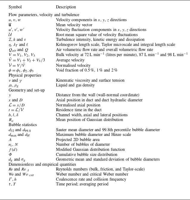


 Open access